Willingness to Pay for Clean Air:

Evidence from Air Purifier Markets in China

Koichiro Ito

University of Chicago and NBER

Shuang Zhang

⇤

University of Colorado Boulder

This version: June 16, 2016

Abstract

We develop a framework to estimate willingness to pay (WTP) for clean air from defensive

investment. Applying this framework to product-by-store level scanner data on air purifier

sales in China, we provide among the first revealed preference estimates of WTP for clean

air in developing countries. A spatial discontinuity in air pollution created by the Huai River

heating policy enables us to analyze household responses to long-run exposure to pollution. Our

model allows heterogeneity in preference parameters to investigate potential heterogeneity in

WTP among households. We show that our estimates provide important policy implications for

optimal environmental regulation.

⇤Ito: Harris School of Public Policy, University of Chicago, and NBER (e-mail: ito@uchicago.edu). Zhang: De-partment of Economics, University of Colorado Boulder (e-mail: shuang.zhang@colorado.edu). For helpful comments,we thank Douglas Almond, Marshall Burke, Steve Cicala, Thomas Covert, Richard Freeman, Michael Greenstone,Rema Hanna, Kelsey Jack, Ryan Kellogg, Michael Kremer, Shanjun Li, Mushfiq Mobarak, Matt Neidell, PaulinaOliva, Nick Ryan, Nick Sanders, Joseph Shapiro, Christopher Timmins, Tom Wollmann, participants in the NBEREnvironmental and Energy Economics Program Meeting, NBER/BREAD Development Meeting, the NBER ChineseEconomy Meeting and the SIEPR Conference, and seminar participants at Harvard, MIT, Cornell, Colorado Boulder,IGC, University of Chicago, University of Illinois at Urbana Champaign, University of Tokyo, University of Calgary,Georgetown, and the RIETI. We thank Ken Norris, Jing Qian and Chenyu Qiu for excellent research assistance.

1 Introduction

Air quality is remarkably poor in developing countries, and severe air pollution is imposing a

substantial health and economic burden on billions of people. For example, the annual average

exposure to fine particulate matter in China was more than five times higher than that of the US

in 2013 (Brauer et al., 2016). Such high levels of air pollution cause large negative impacts on a

variety of economic outcomes, including infant mortality (Jayachandran, 2009; Arceo et al., 2012;

Greenstone and Hanna, 2014), life expectancy (Chen et al., 2013), and labor supply (Hanna and

Oliva, 2015). For this reason, policymakers and economists consider air pollution to be one of the

first-order obstacles to economic development.

However, a large economic burden of air pollution does not necessarily imply that existing

environmental regulations are not optimal. Optimal environmental regulation depends on the

extent to which individuals value air quality improvements—that is, their willingness to pay (WTP)

for clean air (Greenstone and Jack, 2013). If WTP for clean air is low, the current level of air

pollution can be optimal because social planners prioritize economic growth over environmental

regulation. On the other hand, if WTP is high, the current stringency of regulations can be far

from optimal. Therefore, WTP for clean air is a key parameter when considering the tradeo↵s

between economic growth and environmental regulation. Despite the importance of this question,

the economics literature provides limited empirical evidence. This is primarily because obtaining a

revealed preference estimate of WTP for clean air is particularly challenging in developing countries

because of limited availability of high quality data and a lack of readily available exogenous variation

in air quality that are necessary for empirical analysis.

In this paper, we provide among the first revealed preference estimates of WTP for clean air in

developing countries. Our approach is based on the idea that demand for home-use air purifiers,

a main defensive investment for reducing indoor air pollution, provides valuable information for

the estimation of WTP for air quality improvements. We begin by developing a random utility

model in which consumers purchase air purifiers to reduce indoor air pollution. A key advantage

of analyzing air purifier markets is that one of the product attributes—high-e�ciency particulate

arrestance (HEPA)—informs both consumers and econometricians of the purifier’s e↵ectiveness to

reduce indoor particulate matter. The extent to which consumers value this attribute, along with

1

the price elasticity of demand, reveals their WTP for indoor air quality improvement.

We apply this framework to scanner data on market transactions in air purifier markets in

Chinese cities. At the retail store level, we observe product-level information on monthly sales,

monthly average price, and detailed product attributes. The product attributes include the infor-

mation on each purifier’s e↵ectiveness to reduce indoor air pollution. Our data cover January 2006

through December 2012. The dataset provides comprehensive transaction records of 395 air purifier

products for some of the most polluted cities in the world. To our knowledge, this paper is the first

study to exploit these transaction data in the Chinese air purifier markets to examine consumers’

WTP for air quality. We also collect pollution data from air pollution monitors and micro data on

demographics from the Chinese census to compile a dataset that consists of air purifier sales and

prices, air pollution, and demographic characteristics.

The primary challenge for our empirical analysis is that two variables in the demand estima-

tion—pollution and price—are likely to be endogenous. To address the endogeneity of air pollution,

we use a spatial regression discontinuity (RD) design, which exploits discontinuous valuation in air

pollution created by a policy-induced natural experiment at the Huai River boundary. The so-called

Huai River heating policy provided city-wide coal-based heating for cities north of the river, which

generated substantially higher pollution levels in the northern cities (Almond et al., 2009; Chen

et al., 2013). The advantage of this spatial RD approach is twofold. First, it allows us to exploit

plausibly exogenous policy-induced variation in air pollution. Second, the policy-induced variation

in air pollution has existed since the 1950s. This natural experiment provides long-run variation in

air pollution, which enables us to examine how households respond to long-lasting, not transitory,

variation in pollution.

To address the endogeneity of prices, we combine two approaches. First, we observe data from

many markets (cities) in China, and therefore we are able to include both product fixed e↵ects and

city fixed e↵ects. These fixed e↵ects absorb product-level unobserved demand factors and city-level

demand shocks. The remaining potential concern is product-city level unobserved factors that are

correlated with prices by product and city. We construct an instrumental variable, which measures

the distance from each product’s manufacturing plant (or its port if the product is imported) to

each market, with the aim of capturing variation in transportation cost, which is a supply-side cost

shifter.

2

We first present visual and statistical evidence that the level of air pollution (PM10) is dis-

continuously higher in cities north of the Huai River. A key prediction from our demand model

is that if households value clean air, the market share for HEPA purifiers—that is, purifiers that

can reduce indoor particular matter—should be higher in cities north of the river boundary. Our

second empirical analysis shows that there is indeed a discontinuous and substantial increase in the

market share of HEPA purifiers in the north. We estimate local linear regression for the RD design

and find that the WTP for removing the amount of PM10 generated by the Huai River policy for

five years is USD 190. Third, we estimate that the marginal WTP for removing 1 ug/m3 of PM10

for five years is USD 4.40. We show that our RD estimates are robust to using a range of di↵erent

bandwidths and local quadratic estimation. Fourth, to learn about the distribution of WTP, we

relax a few assumptions on standard logit demand estimation and estimate a random-coe�cient

logit model. The random-coe�cient logit model allows us to estimate potentially heterogeneous

preference parameters for pollution and price. We find substantial heterogeneity that can be ex-

plained by observed and unobserved factors. Our results indicate that the marginal WTP ranges

from USD 0 to over USD 15 among households in our sample and that higher-income households

have significantly higher marginal WTP for clean air compared to lower-income households.

This study provides three primary contributions to the literature and ongoing policy discussions.

First, we develop a framework to estimate WTP for clean air based on defensive investment on

market products. Earlier studies on avoidance behavior on pollution examine whether individuals

take avoidance behavior in response to pollution exposure.1 A key question in the recent literature is

whether researchers can obtain monetized WTP for environmental quality from observing defensive

behavior. Earlier theoretical work in environmental economics emphasizes that defensive investment

on market products can be useful to learn about the preferences for environmental quality (Braden

et al., 1991). However, few existing studies attempt to provide a framework to connect this economic

theory with market data for empirical analysis.2 Our paper compliments the literature by providing

1Earlier studies on avoidance behavior against pollution find that people do engage in defensive investment againstpollution. For evidence in the US, see Neidell (2009); Zivin and Neidell (2009); Zivin et al. (2011). For evidence inChina, see Mu and Zhang (2014); Zheng et al. (2015). For evidence in other developing countries, see Madajewiczet al. (2007); Jalan and Somanathan (2008). A key question in the recent literature is whether researchers canestimate WTP for improvements in environmental quality from observing defensive investment in markets.

2There are two recent papers that are most relevant to our study in the sense that our approach and the approachestaken by the following papers are broadly categorized by the household production approach. Kremer et al. (2011)uses a randomized control trial (RCT) in Kenya to estimate the WTP for water quality. Deschenes et al. (2012) usemedical expenditure data in the United Sates to learn about the cost of air pollution and the benefit of air quality

3

a framework that can be applicable to market-level sales and price data, which are available in

a variety of product markets in many countries through scanner data from manufacturers and

retailers.3

The second contribution is that our analysis provides empirical evidence of an important “miss-

ing piece” in the literature on air pollution in developing countries. Greenstone and Jack (2013)

suggest that few studies have attempted to develop revealed preference estimates of WTP for envi-

ronmental quality in developing countries, despite the fact that recent pollution concentrations in

these countries are far above those ever recorded in the US. The extrapolation of WTP estimators

from studies in developed countries is unlikely to be valid because pollution and income levels are

substantially di↵erent among developed and developing countries. We fill this gap by providing re-

vealed preference estimates of WTP for air quality in China. Our estimates are particularly useful

because the identification comes from long-run exposure to air pollution induced by the Huai River

policy. This is informative for WTP in the developing world where a large part of pollution is not

presented as “on-and-o↵ shocks”.

Finally, our findings provide important policy implications for ongoing discussions in energy

and environmental regulation in developing countries. Developing country governments recently

proposed and implemented interventions to combat air pollution problems. For example, Chinese

Premier Li Keqiang declared “War Against Pollution” to reduce emissions of PM10 and PM2.5

and has proposed various reforms in energy and environmental policies (Zhu, 2014). China has

also made a commitment to address global climate change, as featured by the New York Times

in April 2016 (Davenport, 2016). For example, policies include reforming the Huai River heating

policy and the launch of a national cap-and-trade program on carbon emissions in 2017. A key

question is whether implementing such policies enhances welfare. In the policy implication section

of this paper, we provide an evaluation of the recent reform of the Huai River heating policy as an

example to illustrate how estimates on the WTP for clean air can be used to examine the welfare

implications of energy and environmental policies.

regulation.3There are a few more related studies. Berry et al. (2012); Miller and Mobarak (2013) use randomized controlled

trials to estimate WTP for water filters and cook stoves per se instead of WTP for improvements in environmentalquality. Consumer behavior in housing markets is usually not considered to be “avoidance behavior”, but Chay andGreenstone (2005) is related to our study in the sense that they provide a quasi-experimental approach to estimateWTP for clean air.

4

2 Air pollution, Air Purifiers, and the Huai River Policy in China

In this section, we provide background information on air pollution in Chinese cities, air purifier

markets in China, and the Huai River policy, which are key to our empirical analysis.

2.1 The Main Pollutant in Chinese Cities

Among ambient pollution measures, fine particulate matter has most consistently shown an adverse

e↵ect on human health in recent medical research (Dockery et al. 1993, Pope et al. 2009 and

Correia et al. 2013). Additionally, particulate matter is mostly concentrated in developing countries.

According to a global map of satellite-derived PM2.5 (particulate matter with a diameter of 2.5

micrometers or less), Northern and Eastern China, and Northern India are the most polluted regions

in the world (Van Donkelaar et al., 2010).

Particular matter is the main air pollutant in Chinese cities. Since 2000, the Chinese Ministry

of Environmental Protection (MEP) has released a daily air pollution index (API) for 120 cities.

In each city, a number of monitors record hourly concentration measures of three air pollutants:

PM10 (particulate matter with a diameter of 10 micrometers or less), SO2 and NO2. Daily API is

converted from the pollutant with the highest daily average value. The API value scales from 0 to

500: the higher the value, the greater the level of air pollution. For example, an API value of 0 to

50 represents excellent air while an API value over 300 represents heavily polluted air. When the

API is above 50, the MEP reports the specific type of pollutant from which the API was converted.

During 2006-2012, the main pollutant was PM10, followed by SO2 and NO2 with respective shares

of 91%, 8.9%, and 0.15% of the total days in our sample of cities The o�cial API, based on ambient

PM10 for most days, is the only accessible pollution information for Chinese citizens during our

sample period.4 Both daily API level and the main pollutant type are reported to local residents

by city weather channels, radio and newspapers.

2.2 Air Purifiers

A key advantage of analyzing air purifier markets is that one of the product attributes—high-

e�ciency particulate arrestance (HEPA)—informs both consumers and econometricians of the pu-

4The Chinese government started to report PM2.5 in 2014. We focus on the period 2006 to 2012 because of theavailability and representativeness of our air purifier data for this period.

5

rifier’s e↵ectiveness to reduce indoor particulate matter. According to the US Department of

Energy, a HEPA air purifier removes at least 99.97% of particles of 0.3 micrometer or larger in di-

ameter (DOE, 2005). It is even more e↵ective for larger particles such as PM2.5 and PM10. Recent

clinical studies find that the use of HEPA purifiers in various settings provides improvements in

health, including reduced asthma symptoms and asthma-related health visits among children, lower

marker levels of inflammation and heart disease, and reduced incidences of invasive aspergillosis

among adults (Abdul Salam et al., 2010; Allen et al., 2011; Lanphear et al., 2011). In the Chinese

air purifier markets, consistent with the US Department of Energy standards, air purifier manu-

facturers and retail stores explicitly advertise that a HEPA purifier can remove more than 99% of

particle matter larger than 0.3 micrometers.

In Chinese cities, HEPA purifiers have approximately half of the market share, and non-HEPA

purifiers have another half of the market share. Non-HEPA purification technologies are designed to

remove other target pollutants, not particulate matter. Activated carbon absorbs volatile organic

compounds (VOCs), but it does not remove particles. A catalytic converter is e↵ective in removing

VOCs and formaldehyde. An air ionizer generates electrically charged air or gas ions, which attach

to airborne particles that are then attracted to a charged collector plate. However, there are no

specific standards for air ionizers, and they also produce ozone and other oxidants as by-products. A

study by Health Canada finds that a residential ionizer only removes 4% of indoor PM2.5 (Wallace,

2008).

2.3 The Huai River Policy and its Recent Reform

In 1958, the Chinese government decided to provide a centralized heating system. Because of

budget constraints, the government provided city-wide centralized heating to northern cities only

(Almond et al., 2009). Northern and southern China are divided by a line formed by the Huai River

and Qinling Mountains as shown in Figure 1. The government used this line because the average

January temperature is roughly 0° Celsius along the line, and the line is not a border for other

administrative purposes (Chen et al., 2013). Cities to the north of the river boundary have received

centralized heating in every winter. In contrast, cities in the south have not had a centralized

heating supply from the government.

The centralized heating supply in the north relies on coal-fired heating systems. Two-thirds

6

of heat is generated by heat-only hot water boilers for one or several buildings in an apartment

complex, and the remaining one-third is generated by combined heat and power generators for the

larger areas of each city. This system is inflexible and energy ine�cient. Consumers have no means

to control their heat supply and, until recently, there has been no measurement of heat consumption

at the consumer level. The incomplete combustion of coal in the heat generation process leads to

the release of air pollutants, particularly particulate matter. Because most heat is generated by

boilers within an apartment complex, the pollution from coal-based heating remains largely local.

Almond et al. (2009) find that the Huai River policy led to higher total suspended particulate

(TSP) levels in the north. Chen et al. (2013) further find that the higher pollution levels created

by the policy led to a loss of 5.5 years of life expectancy in the north.

The heating supply in the north has been consistent since the 1950s while the payment system

under the policy underwent an important reform in 2003. Prior to 2003, free heating was provided

to residents in the north, and employers or local governments were responsible for the payment of

household heating bills (WorldBank, 2005). The payment system was designed under the centrally

planned economy under which the public sector employment dominated the labor market. However,

during China’s transition to a market economy, heating billing became a practical problem. The

size of the private sector has increased dramatically since the 1990s, and employers in the private

sector have not been required to pay heating bills. Additionally, many public sector employees have

moved out of public housing and have purchased homes in the private market, which complicated

the payment of heating bills by public sector employers.

In July 2003, the Chinese government issued a heating reform. The reform changed the payment

system from free provision to flat-rate billing (WorldBank, 2005). Individual households became

responsible for the payment of their own heating bills each season, which is a fixed charge per square

meter of floor area for the entire season ,regardless of actual heating usage. Whether a heating

subsidy is provided by employers varies by sector. In the public sector, former in-kind transfers

were changed to a transparent payment for heating added to the wage. In contrast, private sector

employers were not explicitly required to provide a heating subsidy to their employees. In the

2005 census, 21% of the labor force was in the urban public sector in the 81 cities in our sample,

suggesting that only a small percentage of employees receive a heating subsidy following the reform.

Our analysis focuses on to period from 2006 to 2012, after the 2003 reform on heating billing.

7

We summarize the comparison of winter heating between the north and the south. First, winter

heating is provided in the same way after the reform. The centralized city-wide heating supply

in the north remains the same, where households have little option other than the centralized

coal-based heating that generates higher pollution levels. In the south, households choose their

own methods of staying warm in winter, including using the heating function of air conditioners,

space heaters, heated blankets, etc. Second, heating costs in the north have changed since the 2003

reform. Northern households no longer enjoy free heating and instead have to pay a substantial

proportion of their heating bills from the centralized heating while households in the south continue

to pay for the heating methods of their choice. We collected heating costs in 20 cities within three

degrees of latitude relative to the Huai River boundary and find that household heating costs in

the north are comparable to, or could even be higher than, those in the south.5

3 Data and Descriptive Statistics

We compile a dataset from four data sources—air purifier market data, air pollution data, manu-

facturing/importing location data for each product, and demographic information from the 2005

Chinese census micro data. In this section, we describe each data source and provide descriptive

statistics.

3.1 Air Purifier Data

We use air purifier sales transaction data collected by a marketing firm in China from January 2006

through December 2012 for 81 cities. The company collected product-store-level scanner data on

monthly sales, monthly average price, and product attributes. The data cover a network of major

department stores and electrical appliance stores, which account for over 80% of all in-store sales.

During the period 2006 to 2012, in-store sales consisted of over 95% of overall purifier sales. The

5For example, in Xi’an, a city within one degree of latitude north of the Huai River, the price of heating persquare meter per winter is USD 3.9. For an apartment of 100 square meters, the household pays USD 390. Theaverage subsidy in public sector is USD 177 per employee, and the number of public employees per household is 0.32according to the 2005 population census. The average amount of subsidy per household is USD 57. Therefore, anaverage household’s out-of-pocket payment is USD 333. In southern cities, space heaters and heated blankets are themost common choices that could cost USD 150 to 200 including the purchasing of these devices and the electricitybill in winter for a similar size home. If a household chooses a more expensive option, air conditioning, the electricitybill for three months in winter could be approximately USD 240 to 280 and the entire cost depends on the price ofthe air conditioners, which varies to a large extent.

8

marketing firm provided product-level data for in-store sales only. The share of online sales has

started to increase significantly since 2013. Therefore, our empirical analysis focuses on data for

2006 to 2012.

There are 395 products sold by 30 manufacturers in the dataset. The original sales and price data

are at the product-city-store-year-month level. In our empirical analysis, the exogenous variation

in pollution comes from cross-city variation. Therefore, we aggregate the transaction data to the

product-city level. That is, the unit of observation is a product in a city, and the main variables of

interest are the product’s total sales and average price at the city level during 2006-2012. A unique

feature of the dataset is that we observe detailed attributes for each product. The key attribute is

a High E�ciency Particulate Arrestance (HEPA) filter, which enables us to quantify the amount

of particulate matter that a product can remove.

Finally, to address the endogeneity of prices in our empirical analysis, we construct an instru-

mental variable, which measures the distance from each product’s manufacturing plant (or its port

if the product is imported) to each market. The distance measure captures the variation in the

transportation cost, which is a supply-side price shifter. For each product, we geo-coded the loca-

tion of its manufacturing plant if it is domestically produced, or the location of the importing port

if it is imported. Around 16% of products are imported. We then calculate the distance (km) from

the city where the product is sold to its manufacturing plant for domestically produced products

and to the port for imported products.

3.2 Pollution Data

The o�cial air pollution index (API) is the only accessible air pollution information for Chinese

citizens during the period of this study. We obtain daily API data for each city in our sample for

2006-2012 from the Chinese Ministry of Environmental Protection (MEP). In addition to the API

level, the data source discloses the type of pollutant from which the API was taken from on days

when the air quality is not excellent (API is above 50). This information is also disclosed to the

public. During the sample period, the main pollutant was PM10 for 91% of the days.

The conversion from the concentration of each pollutant to API is based on a known nonlinear

function. For the days that PM10 is reported as the main pollutant, we use the o�cial formula

from the Chinese MEP to convert daily API to daily PM10. We then calculate the average daily

9

PM10 for the winter months (December to March) and non-winter months (April to November) at

the city level. We calculate PM10 for these two seasons separately because the centralized heating

in the north of the Huai River is turned on in late November and turned o↵ at the end of March.

We are cautious in using the API data because recent studies find evidence of underreporting

of API at the margin of 100 (Chen et al. 2012, Ghanem and Zhang 2014). The manipulation

is motivated by the blue sky award, which defines a day with an API below 100 as a blue sky

day and links the number of annual blue sky days to the annual performance evaluation of city

governments. For our analysis, we investigate the extent to which potential manipulation a↵ects

the average API level for cities for the period 2006 to 2012. In the online appendix, we perform

McCrary density tests (McCrary 2008) on daily API data to test potential manipulation and then

estimate the e↵ects of the manipulation on the average level of API at the city level. In Figure A.5

in the appendix, we find that potential manipulation changes the city-level average API for our

sample period by a negligible amount. This is because the manipulation occurs only at the margin

of 100 and therefore, it has a minimal e↵ect on the average API over a long trem.

3.3 Demographic Data

We compile demographic data from two sources. First, we obtain city-year measures on population

and GDP per capita from City Statistical Yearbooks in 2006-2012. Second, we obtain individual-

level micro data from the 2005 census. For each city, the dataset includes demographic variables

for a random sample of individuals. We use household-level income data to create the empirical

distribution of household annual income for each city, which we use in our empirical analysis.

We also aggregate the census data to calculate some additional city-level demographic variables

including average years of schooling and the percentage of individuals who have completed college.

3.4 Summary Statistics

Table 1 reports summary statistics. In Panel A, we show the summary statistics of our air purifier

data at the product level. In our dataset, there are 395 products manufactured by 30 manufactures,

including domestic and foreign companies. Of the 395 products, 206 products, or 52% of all

products, have a HEPA filter. We report product-level summary statistics for all products in

column 1, HEPA purifiers in column 2, and non-HEPA purifiers in column 3. For each variable, we

10

also calculate the di↵erence in the means between HEPA purifiers and non-HEPA purifiers and the

standard errors for the di↵erences by clustering at the manufacturer level in column 4. Although

we observe substantial heterogeneity for each variable at the product level, the di↵erence in the

means between HEPA and non-HEPA purifiers is statistically insignificant for sales, market share,

other product attributes such as humidifying and room coverage, the distance to the factory or the

port, and the frequency of filter replacement. In contrast, the di↵erence is statistically significant

for the price of purifiers and the price of replacement filters. On average, HEPA purifiers are USD

112 more expensive than non-HEPA purifiers, and the di↵erence is statistically significant at the

10% level. HEPA replacement filters are also USD 20 more expensive than non-HEPA replacement

filters, and the di↵erence is statistically significant at the 10% level.

Panel B and C of Table 1 report summary statistics for our two datasets at the city level—

pollution data and demographic data. The average PM10 in winter months is 115 ug/m3, while

it is 93 ug/m3 in non-winter months. Cities in our dataset have, on average, a population of 2.5

million. The average GDP per capita is USD 8,277. The average years of schooling is 8.36 years,

and the percentage of individuals who have completed college is, on average, 3.6%.

We also use two maps to show the spatial distributions of the cities and manufacturing plants/ports

in our dataset. Figure 1 shows the location of the 81 cities on the China map in our analysis. The

line of Huai River/Qinling Mountains divides China into North and South. Each dot represents

a city in our sample. All cities in our sample are located east of 100 degrees of longitude. The

river line east of 100 degrees of longitude ranges between 32.6 and 34.2 degrees of latitude. In our

spatial RD approach using the Huai River policy, we define a city’s relative latitude north of the

river line. Because the river line has several di↵erent curved segments, we divide the river line into

five segments. In each segment, we measure a city’s relative latitude to the middle point of the

river latitude range. For example, Beijing is located at 39.9 degrees of latitude and 116.3 degrees of

longitude, and the corresponding middle point of the river latitude range is 33.4 degrees. Beijing’s

relative latitude north of the river line is 6.5 (39.9 to 33.4) degrees. Cities in our sample are located

between -12.9 and 14.8 degrees north of the river line. In the appendix, we also show Figure A.1,

which includes the locations of manufacturing plants of domestically produced products and ports

of imported products on the map. Most manufacturing plants and ports are located on the east

coast.

11

4 Demand for Air Purifiers

Our goal is to obtain a revealed preference estimate of WTP for clean air by analyzing demand for

air purifiers. Because air purifiers are di↵erentiated products with multiple attributes, we start with

a random utility model for di↵erentiated products.6 When a consumer purchases an air purifier,

the consumer considers utility from the product attributes and disutility from the price. For our

objective, an advantage of analyzing air purifier markets is that one of the product characteristics—

high-e�ciency particulate arrestance (HEPA)—informs consumers and researchers of the purifier’s

e↵ectiveness to reduce indoor particulate matter. The intuition behind our approach is that the

extent to which consumers value this characteristic, along with the price elasticity of demand,

provides useful information on their WTP for indoor air quality improvements.

Consider that consumer i in city c has ambient air pollution xc (particulate matter). The

consumer can purchase air purifier j at price pjc to reduce indoor air pollution by xjc = xc · ej .

We denote purifier j’s e↵ectiveness to reduce indoor particulate matters by ej 2 [0, 1]. We observe

markets for c = 1, ..., C cities with i = 1, ..., Ic consumers. The conditional indirect utility of

consumer i from purchasing air purifier j at city c is:

uijc = �ixjc + ↵ipjc + ⌘j + �c + ⇠jc + ✏ijc, (1)

where xjc is the improvement in indoor air quality conditional on the purchase of product j, pjc is the

price of product j in market c, ⌘j is product fixed e↵ects that capture utility gains from unobserved

and observed product characteristics, �c is city fixed e↵ects, ⇠jc is a product-city specific demand

shock, and ✏ijc is a mean-zero stochastic term. �i indicates the marginal utility for clean air, and

↵i indicates the marginal disutility of price. The functional form for the utility function assumes

that each variable, including the error term, enter the utility function linearly.

Air purifiers usually run for five years and require filter replacement several times within five

years. We assume that consumer i considers utility gains from purifier j for five years and pjc as

a total cost including the upfront and running cost.7 This approach abstracts from the interesting

6For more detailed discussion on randomm utility models for di↵erentiated products and their estimation, see Berry(1994); Berry et al. (1995); Goldberg (1995); Nevo (2001); Kremer et al. (2011); Knittel and Metaxoglou (2013).

7This approach also implicitly assumes that consumers respond to the monetary value of an upfront cost andrunning costs in the same way when they purchase air purifiers. For example, if consumers are myopic, they canbe more responsive to an upfront cost than running costs. While we cannot rule out this possibility, recent studies

12

possibility that consumers may consider the dynamics of product entries and make a dynamic

decision. Unfortunately, it is not possible to examine such a dynamic decision in the context

of our empirical setting. While we have monthly sales and price data, the exogenous variation in

pollution comes from purely cross-sectional variation as opposed to time-series variation. Therefore,

our empirical approach focuses on cross-sectional variation in pollution and purchasing behavior,

which has to abstract from potential dynamic discrete choices.

We assume that the error term ✏ijc is distributed as a Type I extreme-value function. We

then consider both a standard logit model and a random-coe�cient logit model. A standard logit

model assumes that the preference parameters do not vary by i. The attractive feature of this

approach is that the random utility model in equation (1) leads to a linear equation. The linear

equation can be estimated by linear GMM estimation with instrumental variables for pollution

and price. A random-coe�cient logit model allows the preference parameters to vary by household

i through observable and unobservable factors. This feature comes at a cost—random-coe�cient

logit estimation involves nonlinear GMM estimation for a highly nonlinear objective function. In

this paper, we use both approaches to estimate WTP for clean air.

4.1 A Logit Model

We begin with a standard logit model. Suppose that �i = � and ↵i = ↵ for all consumer i and that

the error term ✏ijc is distributed as a Type I extreme-value function. Consumer i purchases purifier

j if uijc > uikc for 8k 6= j. Then, the market share for product j in city c can be characterized by8

sjc =exp(�xjc + ↵pjc + ⌘j + �c + ⇠jc)PJ

k=0 exp(�xkc + ↵pkc + ⌘k + �c + ⇠kc). (2)

The outside option (j = 0) is not to buy an air purifier. We make a few assumptions to construct

the market share for the outside option (s0c). We assume that the number of households in city c

are potential buyers, and that each household purchases one or zero air purifier during our sample

period. Then, s0c can be calculated by the di↵erence between the number of households in city c and

show empirically that consumers are not myopic concerning the running costs of durable goods (Busse et al., 2013).When calculating the total cost of a purifier, we do not consider future discount rates in its running cost. However,including discount rates changes the total cost only by a small amount and, therefore, we find that it does not havea significant e↵ect on our empirical findings.

8See Berry (1994) for the proof and more detailed discussions.

13

the total number of sales in city c. Our second assumption is that x0c = 0. That is, if consumers do

not buy an air purifier, they are exposed to indoor pollution that is equal to ambient air pollution.

Note that for the standard logit estimation, the assumptions on the outside option are not required

when we include city fixed e↵ects. City fixed e↵ects absorb observable and unobservable variation

at the city level. For completeness, we include the log of market share for the outside option (s0c )

in the equation below, but the term will be absorbed by city fixed e↵ects. The log market share for

the outside options is ln s0c = � ln⇣PJ

k=0 exp(�xkc + ↵pkc + ⌘k + ⇠kc)⌘. The di↵erence between

the log market share for product j and the log market share for the outside options is,

lnsjc � lns0c = �xjc + ↵pjc + ⌘j + �c + ⇠jc (3)

where � is the marginal utility for clean air, and ↵ is the marginal disutility from price. The

marginal willingness to pay (MWTP) for one unit of indoor air pollution reduction can be obtained

by ��/↵.

We interpret that our estimate of ��/↵ provides a lower bound of MWTP for one unit of indoor

pollution reduction. First, our approach assumes that indoor air pollution levels in the absence of

air purifiers are equal to ambient pollution levels. Recent engineering studies show that, on average,

indoor pollution levels are lower than outdoor pollution levels in China.9 One approach we could

take is to rely on an engineering estimate of the indoor-outdoor air pollution ratio, which would

produce slightly larger estimates for MWTP. However, because we want to be as conservative as

possible, we assume that indoor air pollution levels are equal to outdoor pollution levels, which

is likely to underestimate the MWTP. Second, households may have limited information on the

negative health e↵ects of air pollution and, therefore, are likely to underestimate the health risk.

If this is the case, our MWTP estimate can be underestimated compared to the case in which

consumers are well-informed of the negative health e↵ects of air pollution. Third, if the running

costs of HEPA purifiers are higher because using HEPA filters costs more electricity, our MWTP

estimate without accounting for the di↵erence in the running costs could be underestimated.

An advantage of studying air purifier markets is that ej (purifier j’s e↵ectiveness to reduce

indoor particulate matters) is well-known for consumers. As we explained in Section 2.2, if a

9A study from Tsinghua University finds that, in Beijing, on average, the indoor concentration of PM2.5 is 67%of the outdoor concentration of PM2.5. See The People’s Daily, April 23, 2015 (Zhang, 2015).

14

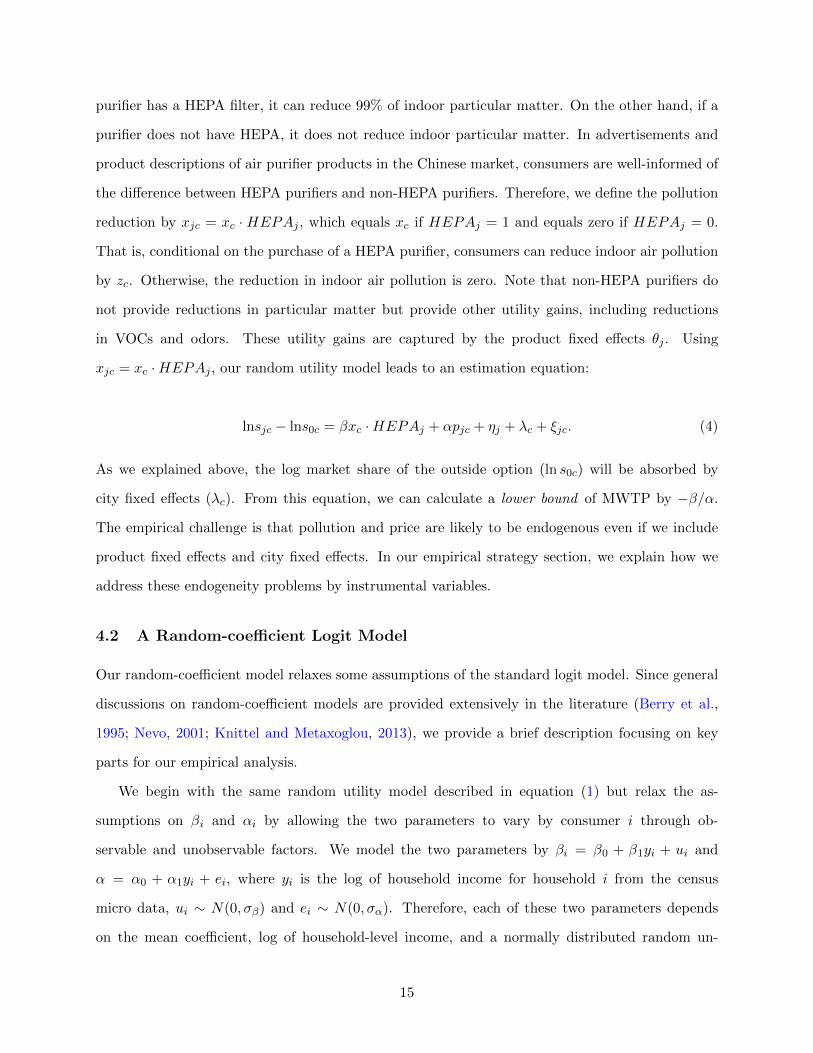
purifier has a HEPA filter, it can reduce 99% of indoor particular matter. On the other hand, if a

purifier does not have HEPA, it does not reduce indoor particular matter. In advertisements and

product descriptions of air purifier products in the Chinese market, consumers are well-informed of

the di↵erence between HEPA purifiers and non-HEPA purifiers. Therefore, we define the pollution

reduction by xjc = xc ·HEPAj , which equals xc if HEPAj = 1 and equals zero if HEPAj = 0.

That is, conditional on the purchase of a HEPA purifier, consumers can reduce indoor air pollution

by zc. Otherwise, the reduction in indoor air pollution is zero. Note that non-HEPA purifiers do

not provide reductions in particular matter but provide other utility gains, including reductions

in VOCs and odors. These utility gains are captured by the product fixed e↵ects ✓j . Using

xjc = xc ·HEPAj , our random utility model leads to an estimation equation:

lnsjc � lns0c = �xc ·HEPAj + ↵pjc + ⌘j + �c + ⇠jc. (4)

As we explained above, the log market share of the outside option (ln s0c) will be absorbed by

city fixed e↵ects (�c). From this equation, we can calculate a lower bound of MWTP by ��/↵.

The empirical challenge is that pollution and price are likely to be endogenous even if we include

product fixed e↵ects and city fixed e↵ects. In our empirical strategy section, we explain how we

address these endogeneity problems by instrumental variables.

4.2 A Random-coe�cient Logit Model

Our random-coe�cient model relaxes some assumptions of the standard logit model. Since general

discussions on random-coe�cient models are provided extensively in the literature (Berry et al.,

1995; Nevo, 2001; Knittel and Metaxoglou, 2013), we provide a brief description focusing on key

parts for our empirical analysis.

We begin with the same random utility model described in equation (1) but relax the as-

sumptions on �i and ↵i by allowing the two parameters to vary by consumer i through ob-

servable and unobservable factors. We model the two parameters by �i = �0 + �1yi + ui and

↵ = ↵0 + ↵1yi + ei, where yi is the log of household income for household i from the census

micro data, ui ⇠ N(0,��) and ei ⇠ N(0,�↵). Therefore, each of these two parameters depends

on the mean coe�cient, log of household-level income, and a normally distributed random un-

15

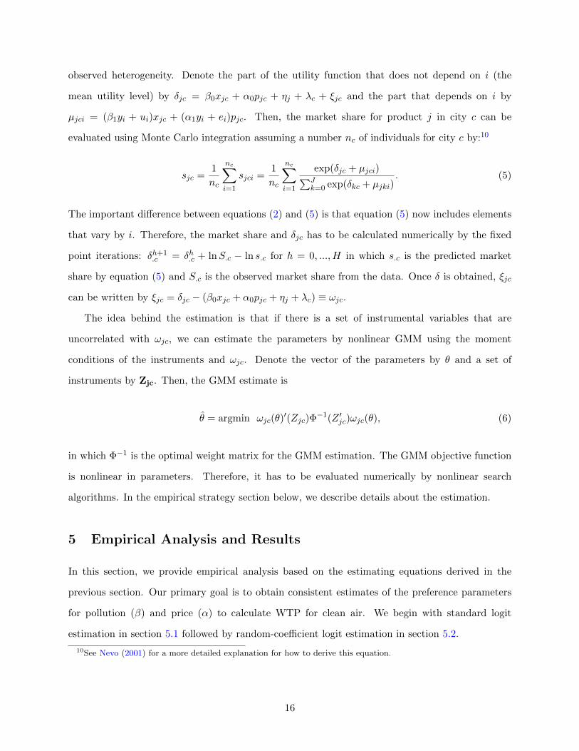
observed heterogeneity. Denote the part of the utility function that does not depend on i (the

mean utility level) by �jc = �0xjc + ↵0pjc + ⌘j + �c + ⇠jc and the part that depends on i by

µjci = (�1yi + ui)xjc + (↵1yi + ei)pjc. Then, the market share for product j in city c can be

evaluated using Monte Carlo integration assuming a number nc of individuals for city c by:10

sjc =1

nc

ncX

i=1

sjci =1

nc

ncX

i=1

exp(�jc + µjci)PJk=0 exp(�kc + µjki)

. (5)

The important di↵erence between equations (2) and (5) is that equation (5) now includes elements

that vary by i. Therefore, the market share and �jc has to be calculated numerically by the fixed

point iterations: �h+1.c = �h.c + lnS.c � ln s.c for h = 0, ..., H in which s.c is the predicted market

share by equation (5) and S.c is the observed market share from the data. Once � is obtained, ⇠jc

can be written by ⇠jc = �jc � (�0xjc + ↵0pjc + ⌘j + �c) ⌘ !jc.

The idea behind the estimation is that if there is a set of instrumental variables that are

uncorrelated with !jc, we can estimate the parameters by nonlinear GMM using the moment

conditions of the instruments and !jc. Denote the vector of the parameters by ✓ and a set of

instruments by Zjc. Then, the GMM estimate is

✓̂ = argmin !jc(✓)0(Zjc)�

�1(Z 0jc)!jc(✓), (6)

in which ��1 is the optimal weight matrix for the GMM estimation. The GMM objective function

is nonlinear in parameters. Therefore, it has to be evaluated numerically by nonlinear search

algorithms. In the empirical strategy section below, we describe details about the estimation.

5 Empirical Analysis and Results

In this section, we provide empirical analysis based on the estimating equations derived in the

previous section. Our primary goal is to obtain consistent estimates of the preference parameters

for pollution (�) and price (↵) to calculate WTP for clean air. We begin with standard logit

estimation in section 5.1 followed by random-coe�cient logit estimation in section 5.2.

10See Nevo (2001) for a more detailed explanation for how to derive this equation.

16

5.1 Logit Estimation

Our primary empirical challenge is that two variables in the demand estimation—pollution and

price—are likely to be endogenous. In an ideal controlled experiment, one would expose di↵erent

consumers to randomly assigned pollution levels and purifier prices to estimate the demand for

air purifiers in relation to variation in air pollution. In reality, these two variables are unlikely to

be randomly assigned. Air pollution is determined by both observable and unobservable factors.

Therefore, we cannot consider observed pollution levels across di↵erent cities exogenous variation

because of potentially omitted variables. Air purifier prices are also unlikely to be determined

exogenously because unobserved factors in demand are believed to be correlated with price. For

example, suppose that some demand factors are unobservable to econometricians but observable

to firms. If firms have the ability to set prices because of imperfect competition, we expect that

they set prices in response to the unobserved demand factors, which creates correlation between

the price and the error term in our demand estimation.

We address the endogeneity of air pollution by exploiting a regression discontinuity design at

the spatial border of the Huai River as described in section 2.3. This approach provides us a useful

research environment for two reasons. First, it allows us to exploit plausibly exogenous variation

in air pollution created by the natural experiment—the Huai river heating policy. If households

value air quality, our demand model in section 4 predicts that the market share for HEPA purifiers

is discontinuously higher in cities north of the Huai River. Second, the discontinuous di↵erence in

air pollution created by the Huai River policy has existed since the 1950s. Therefore, the natural

experiment provides long-run variation in air pollution, which enables us to examine how households

respond to variation in pollution that is long-lasting rather than transitory.

We address the endogeneity of prices by combining two approaches. First, we use data from

many markets (cities) in China, which allows us to include both product fixed e↵ects and city fixed

e↵ects. These fixed e↵ects absorb product-level and city-level unobserved demand factors. The

remaining potential concern is product-city level unobserved factors that might be correlated with

prices by product and city. To address this concern, we construct an instrumental variable that mea-

sures the distance from each product’s manufacturing plant (or its port if the product is imported)

to each market. This instrument provides variation at the city-product level because manufacturing

17

locations or importing ports are di↵erent between products, and it captures transportation cost of

the product, which is a supply-side cost shifter.

5.1.1 Empirical Strategy

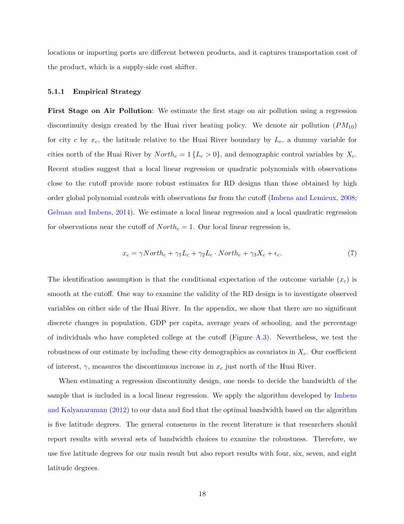
First Stage on Air Pollution: We estimate the first stage on air pollution using a regression

discontinuity design created by the Huai river heating policy. We denote air pollution (PM10)

for city c by xc, the latitude relative to the Huai River boundary by Lc, a dummy variable for

cities north of the Huai River by Northc = 1 {Lc > 0}, and demographic control variables by Xc.

Recent studies suggest that a local linear regression or quadratic polynomials with observations

close to the cuto↵ provide more robust estimates for RD designs than those obtained by high

order global polynomial controls with observations far from the cuto↵ (Imbens and Lemieux, 2008;

Gelman and Imbens, 2014). We estimate a local linear regression and a local quadratic regression

for observations near the cuto↵ of Northc = 1. Our local linear regression is,

xc = �Northc + �1Lc + �2Lc ·Northc + �3Xc + ✏c. (7)

The identification assumption is that the conditional expectation of the outcome variable (xc) is

smooth at the cuto↵. One way to examine the validity of the RD design is to investigate observed

variables on either side of the Huai River. In the appendix, we show that there are no significant

discrete changes in population, GDP per capita, average years of schooling, and the percentage

of individuals who have completed college at the cuto↵ (Figure A.3). Nevertheless, we test the

robustness of our estimate by including these city demographics as covariates in Xc. Our coe�cient

of interest, �, measures the discontinuous increase in xc just north of the Huai River.

When estimating a regression discontinuity design, one needs to decide the bandwidth of the

sample that is included in a local linear regression. We apply the algorithm developed by Imbens

and Kalyanaraman (2012) to our data and find that the optimal bandwidth based on the algorithm

is five latitude degrees. The general consensus in the recent literature is that researchers should

report results with several sets of bandwidth choices to examine the robustness. Therefore, we

use five latitude degrees for our main result but also report results with four, six, seven, and eight

latitude degrees.

18

Finally, recent studies suggest that the local linear regressions should be run with kernel weights

that assign more weights on observations near the cuto↵ (Imbens and Kalyanaraman, 2012; Calonico

et al., 2014). For our main specification, we use a triangular kernel, which is most commonly used

in recent studies. We also estimate our regressions without weights. Because we limit our sample

to observation near the cuto↵, we find that including or excluding weights does not substantially

change the estimation results.

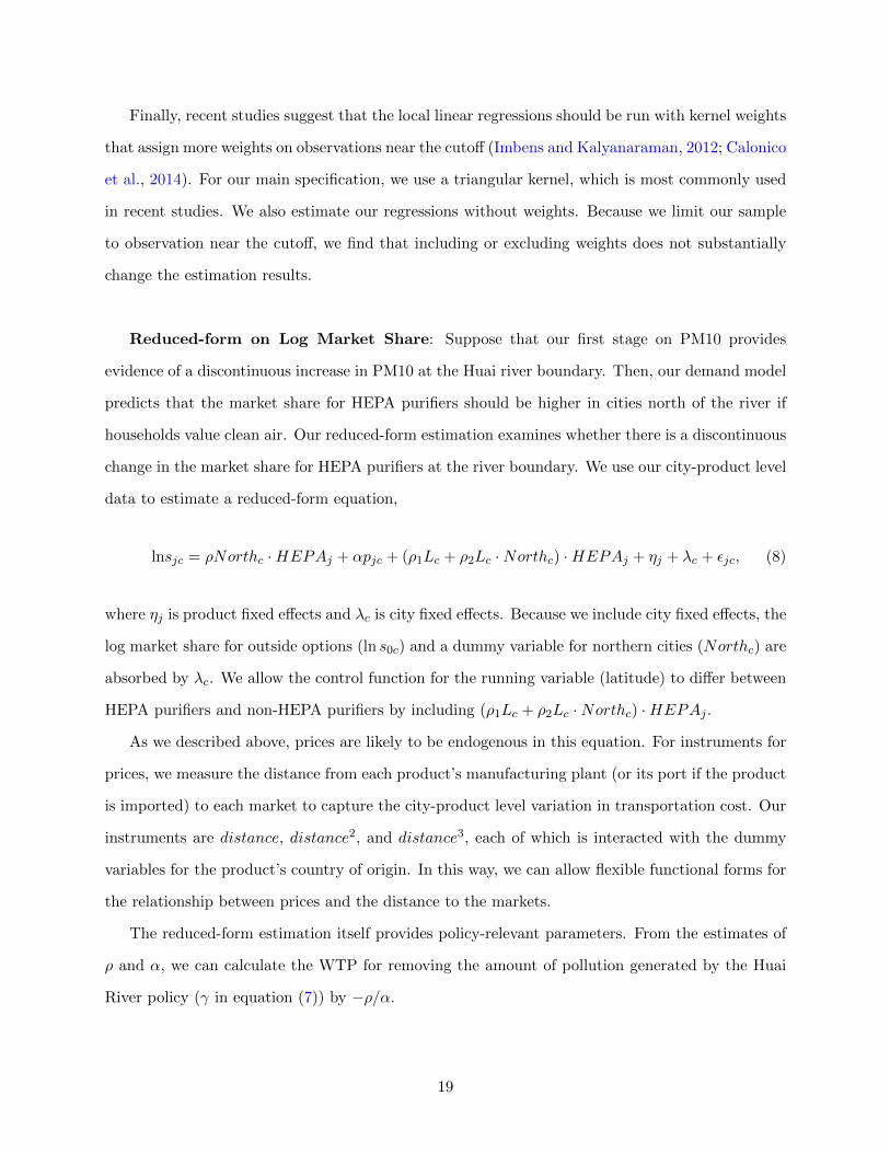
Reduced-form on Log Market Share: Suppose that our first stage on PM10 provides

evidence of a discontinuous increase in PM10 at the Huai river boundary. Then, our demand model

predicts that the market share for HEPA purifiers should be higher in cities north of the river if

households value clean air. Our reduced-form estimation examines whether there is a discontinuous

change in the market share for HEPA purifiers at the river boundary. We use our city-product level

data to estimate a reduced-form equation,

lnsjc = ⇢Northc ·HEPAj + ↵pjc + (⇢1Lc + ⇢2Lc ·Northc) ·HEPAj + ⌘j + �c + ✏jc, (8)

where ⌘j is product fixed e↵ects and �c is city fixed e↵ects. Because we include city fixed e↵ects, the

log market share for outside options (ln s0c) and a dummy variable for northern cities (Northc) are

absorbed by �c. We allow the control function for the running variable (latitude) to di↵er between

HEPA purifiers and non-HEPA purifiers by including (⇢1Lc + ⇢2Lc ·Northc) ·HEPAj .

As we described above, prices are likely to be endogenous in this equation. For instruments for

prices, we measure the distance from each product’s manufacturing plant (or its port if the product

is imported) to each market to capture the city-product level variation in transportation cost. Our

instruments are distance, distance2, and distance3, each of which is interacted with the dummy

variables for the product’s country of origin. In this way, we can allow flexible functional forms for

the relationship between prices and the distance to the markets.

The reduced-form estimation itself provides policy-relevant parameters. From the estimates of

⇢ and ↵, we can calculate the WTP for removing the amount of pollution generated by the Huai

River policy (� in equation (7)) by �⇢/↵.

19

Second Stage on Log Market Share: We estimate the marginal willingness to pay (MWTP)

for clean air by running the following second stage regression:

lnsjc = �xc ·HEPAj + ↵pjc + (�1Lc + �2Lc ·Northc) ·HEPAj + ⌘j + �c + ✏jc, (9)

by using Northc ·HEPAj as the instrument for xc ·HEPAj and the same set of instruments used

in the reduced-form estimation as the instruments for pjc. The identification assumption is that

the instruments are uncorrelated with the error term given the control function and fixed e↵ects.

This estimation allows us to calculate the MWTP for removing one unit of PM10 by ��/↵.

5.1.2 Graphical Analysis

Huai River policy generates a natural experiment in air pollution in the winter months because the

policy-induced pollution comes from centralized heating facilities operating in winter. In Figure 2a,

we show the average PM10 in the winter months (December to March) during 2006-2012 by the

running variable, which is the latitude of cities (Lt). Because few cities are located in the farthest

north and the farthest south, the figure includes cities located within 10 degrees of latitude from the

Huai River boundary. Each plot in the figure shows the average PM10 by 1.5 degrees of latitude.

The vertical line at Lc = 0 indicates the location of the Huai River. Consistent with findings in

previous studies (Almond et al. (2009), Chen et al. (2013)), the figure suggests a discontinuous

increase in PM10 just north of the Huai River. This evidence suggests that the coal-based heating

policy generated higher pollution levels in cities north of the river boundary. We also investigate if a

similar discontinuity in air pollution can be found for non-winter months, when the heating facilities

do not operate. Figure A.2 in the appendix shows that there is no discontinuous change in PM10

levels at the boundary in non-winter months (April to November). This finding provides further

support that the discontinuous increase in pollution presented in Figure 2a is likely generated by

the Huai River policy.

In Figure 2b, we show an analogous RD figure for our outcome variable. That is, Figure

2b presents graphical analysis for the reduced-form regression. We calculate the market share of

HEPA purifiers by 1.5 degrees of latitude. In the south, the market share of HEPA purifiers is

below 60%. The figure indicates that there is a sharp increase in the market share of HEPA at the

20

river boundary, and that the share is over 70% in cities just north of the river. Additionally, the

figure shows no strong trend in the outcome variable by latitude. The relatively flat relationship

between the outcome variable and the running variable suggests that the choice of functional form

for the running variable is unlikely to have a substantial impact on the reduced-form estimation.

5.1.3 Estimation Results

Table 2 shows the results of the first stage estimation. We report the first stage estimation for

PM10 in Panel A. The first two columns show results without demographic controls, and the last

two columns show results with demographic controls. We report our estimates from local linear

regression and local quadratic regression. Without demographic controls, our estimates imply

that there is a discontinuous increase in PM10 of 37 to 39 units at the Huai River boundary.

The magnitude of these estimates is consistent with the visual evidence from Figure 2a. With

demographic controls, the magnitude becomes slightly larger, but the estimates with and without

demographic controls are statistically indi↵erent. Note that the mean PM10 for cities just south of

the Huai River is approximately 115 and jumps by approximately 30% just north of the river.

In Panel B of Table 2, we report the first stage estimation for prices. We include product fixed

e↵ects in all columns. The unit of the distance variable is in 1,000 kilometers (621 miles). The

coe�cient estimates for all columns imply that distance and prices have a nonlinear relationship,

and it is monotonically increasing for the range of distance in the dataset. For example, the result

in columns 1 implies that a hundred kilometer increase (a 62.1 mile increase) in the distance to

the manufacturing plant or importing port is associated with an increase in price of approximately

USD 12 =136.14 · (0.1)� 174.65 · (0.1)2 + 70.22 · (0.1)3. Note that the 10th, 25th, 50th, 75th, and

90th percentiles of the distance variable in our data are 230 km, 550 km, 1,000 km, 1,400 km, and

1,700 km, and that the average price of air purifiers is USD 400. Therefore, the first stage estimates

imply that a considerable amount of variation in prices can be explained by transportation costs

to markets. In columns 3 and 4, we include city fixed e↵ects to control for potentially confounding

factors at the city level. For example, firms possibly set higher prices for cities with higher average

income. The results in these columns imply that the relationship between distance and price is

robust to the inclusion of city fixed e↵ects.

Table 3 shows the reduced-form results in Panel A and the second-stage results in Panel B.

21

We include product fixed e↵ects and city fixed e↵ects. Because we have more instruments than

regressors (an over-identified case), the two-step GMM estimation with the optimal weight matrix

provides a more e�cient estimator than the two-stage least squares (Cameron and Trivedi, 2005).

We use the orthogonality conditions of the instruments to implement the two-step linear GMM

estimation and cluster the standard errors at the city level. Consistent with Figure 2b, the reduced-

form results provide evidence that there is an economically and statistically significant discontinuous

increase in the market share of HEPA purifiers in cities north of the river from both specifications.

We calculate the WTP by �⇢/↵ and obtain its standard error by the delta method. Using local

linear regression, the estimates in column 1 imply that the WTP for reducing the amount of air

pollution generated by the Huai river policy for five years is USD 190 per household. With local

quadratic regression in column 2, the magnitudes of the estimates change slightly, but the estimates

from the two estimation methods are statistically indi↵erent.

Finally, we report the second-stage results in Panel B of Table 3. We use the delta method to

calculate the standard error for ��/↵, which tells us the marginal WTP for reducing one unit of

PM10 for five years. The results for the local linear regression indicate that the MWTP is about

USD 4.4 per household.11

5.1.4 Robustness of the Estimates

We first test the robustness of our main results to bandwidth selection. For the second stage

estimation in Table 4, we use a range of bandwidths between four and eight latitude degrees. We

report the results using local linear regression in Panel A and local quadratic regression in Panel B.

We use triangular kernel for both functional forms. The results imply that our estimates are stable

to a choice of di↵erent bandwidths. We also report in Table A.2 and Table A.3 in the appendix that

estimates of the first stage and reduced form are also robust, consistent with the visual evidence in

Figures 2a and 2b.

A potential concern is that if high-income or better-educated households prefer HEPA purifiers

11Figure A.2 in the online appendix shows that we do not find a discontinuous change in PM10 at the river boundaryfor non-winter months (April to November). This is consistent with the fact that the centralized heating in the north isprovided in winter months only. Nevertheless, we consider the possibility that consumers could purchase air purifiersduring an entire year including non-winter months as a response to higher pollution levels in winter months becauseair purifiers are durable goods. In the online appendix, we test this possibility in Table A.4. The point estimatesin the table suggest that demand for HEPA purifiers in all months has a moderate response to di↵erences in winterPM10, but the response is lower than in winter months.

22

over non-HEPA purifiers for reasons unrelated to air pollution, the interaction term of income and

HEPA, or that of education and HEPA, can be omitted variables. In Table A.1 in the online

appendix, we include the interaction of GDP per capita and HEPA and the interaction of average

schooling and HEPA. We find that the results are similar to our main estimates in Table 3.

5.1.5 Potential Confounding Factors to the Estimation

In this section, we consider potential confounders that could bias our results. First, the RD design

requires that the conditional expectation of potential outcomes are smooth in the running variable

across the river boundary. While potential outcomes are unobservable, we can examine whether

observable variables have discontinuities at the river boundary. In Figure A.3 in the online appendix,

we show that there are no discontinuous changes in demographic variables across the Huai River

boundary.

The second possible concern is sorting of households because of air pollution—households in

the north may migrate to the south to seek cleaner air. This sorting, if it exists, could bias our

estimates. In our case, however, sorting is unlikely to significantly a↵ect our estimates because

of strict migration policies enforced by the Chinese government. Internal migration in China is

strictly constrained by the Hukou system. The hukou, obtained at one’s city of birth, is crucial for

obtaining local social benefits and education opportunities, which makes migration a more costly

decision than migration in countries without restrictions on mobility. The government started to

relax the Hukou system by allowing a few types of migraiotn since the late 1990s, but the migration

rate is still low. We look into migration in the micro-data of the two population census after the

relaxation, the 2000 census and the 2005 census. Indeed, in the 2000 census micro-data, only 0.5

percent of the population in the city of origin within 1.5 latitude degrees north of the Huai river

had migrated to the south. In the 2005 census micro-data, 1 percent of the population in the city

of origin within 1.5 latitude degrees north of the Huai river had migrated to the south. Therefore,

in our case, migration is unlikely to have a significant impact on our estimation.

Third, if there are other policies that use the Huai River boundary, there can be di↵erential

impacts of such policies on households to the north and south of the river boundary. However, as

described in Chen et al. (2013), this line was used to divide the country for heating policy because

the average January temperature is roughly 0° Celsius along the line and has not been used for

23

administrative purposes.

Fourth, we are concerned that the Huai River policy may a↵ect purifier purchases for reasons

unrelated to air pollution. For example, if we consider the heating supply to the north a public

welfare entitlement with subsidized heating costs for northern households, northern households

might have a higher income because of the heating subsidy. We cannot fully rule out this possibility,

but our empirical strategy mitigates this concern for three reasons. First, our estimation includes

city fixed e↵ects. Therefore, if the subsidy for heating increases household wealth, which may

increase demand for purifiers overall (i.e., both HEPA and non-HEPA purifiers), it does not bias

our results. Second, in Table A.1, we find that including the interaction of GDP per capita and

HEPA does not change our main estimate. Third, as we discussed in Section 2.3, the heat reform

in 2003 changed the payment system from free provision to flat-rate billing. Of critical importance

is that northern households must pay a substantial proportion of the total heating bill since 2003.

Therefore, in our analysis during the period 2006 to 2012, the heating subsidy has a minimal e↵ect

on households, although we cannot fully exclude the possibility that the subsidy before 2003 may

have had long-run e↵ects on households during 2006–2012.

A final note is on the availability of HEPA purifier products between the north and south of the

river. If HEPA purifiers are more available in the north because appliance stores supply more of

them compared to non-HEPA purifiers, what we observe in Figure 2b might reflect the di↵erence in

supply. To directly test this concern, in Figure A.4, we plot the fraction of HEPA purifier products

(out of all available purifier products on the market) by 1.5 degrees of latitude relative to the Huai

River. We do not observe a discontinuous jump in the supply of HEPA purifiers just north of the

river boundary.

5.2 Random-coe�cient Logit Estimation

The advantage of the standard logit estimation presented in the previous section is that it can be

estimated by a linear two-stage least squares or a linear GMM method, and therefore, it does not

involve nonlinear estimation. On the other hand, a key assumption in the standard logit model is

that the preference parameters are homogeneous across individuals. That is, we implicitly assume

that the preference for clean air (�) and price (↵) are homogeneous and, hence, the MWTP for

clean air (��/↵) is homogeneous across i.

24

In this section, we relax this assumption and estimate heterogeneity in � and ↵. We model these

parameters by �i = �0 + �1yi + ui and ↵ = ↵0 + ↵1yi + ei, where yi is the log of household-level

income from the census micro data, ui ⇠ N(0,��) and ei ⇠ N(0,�↵). In this way, we model these

two preference parameters for consumer i depend on the mean coe�cient, log of household-level

income, and a normally distributed random error.

5.2.1 Nonlinear optimization algorithms and starting values

Random-coe�cient demand estimation requires nonlinear GMM estimation. The estimation has to

be based on a nonlinear search algorithm with a set of starting values and stopping rules for termi-

nation. Recent studies show caution regarding such numerical optimization and provide guidelines

in assessing robustness of estimation results. For example, Knittel and Metaxoglou (2013) sug-

gest examining 1) conservative tolerance levels for nonlinear searches, 2) di↵erent sets of nonlinear

search algorithms, and 3) many starting values, to analyze whether the estimated local optimum is

indeed the global optimum of the GMM objective function.

We estimate our model with six nonlinear search algorithms (Conjugate gradient, SOLVOPT,

quasi-Newton 1, and quasi-Newton 2, Simplex and Generalized pattern search), a hundred sets of

starting values, and conservative tolerance levels for nonlinear searches. In total, we obtain 600

estimation results to test the robustness of our results. For starting values for nonlinear parameters,

we generate random draws from a standard normal distribution. We set the tolerance level for the

nested fixed-point iterations to 1E�14, and the tolerance level for changes in the parameter vector

and objective function to 1E�04.

5.2.2 Estimation results

Figure 3 shows the box plot of the nonlinear GMM estimation results for each of the six nonlinear

search algorithms with a hundred sets of starting values. The box plot shows the distribution of

the final objective function value for each set of estimation. We use a conventional style of box

plots—the thick vertical line indicates the median, the box shows the 25th and 75th percentiles,

and the dots present outside values. Five of the six search algorithms produce the same minimum

value of the objective function (48.723), which is the dashed vertical line in the figure. Only one

of the algorithms—the conjugate gradient algorithm—does not reach that minimum value. Among

25

the hundred set of starting values, 82% of them reach that minimum objective function value for

Generalized pattern search, 81% for Simplex, 97% for Quasi-Newton 1, 95% for Quasi-Newton 2,

and 92% for Solvopt. This result provides two key implications. First, it is important to test

multiple search algorithms and starting values to ensure that the local minimum in a particular

set of estimation is indeed the global minimum. This is consistent with the caution raised in

recent studies. Second, the fact that the five nonlinear search algorithms reach the same minimum

objective function value provides us strong evidence that the local minimum found at the function

value of 48.723 is likely to be the global minimum of the GMM objective function. Therefore,

we use the estimation result with this minimum objective function value to report the coe�cient

estimates.

Table 5 shows the coe�cient estimates of the random coe�cient model described in equation

(6). As with our standard logit estimation, we use two sets of controls for latitude for our regression

discontinuity design. Column1 uses linear and linear interacted with the indicator variable for cities

in the north side of the Huai River, and column 2 uses quadratic controls for the latitude. The

results provide several key findings for heterogeneity in preference parameters. First, the MWTP for

the median and mean households are USD 5.13 and USD 5.46, which are slightly larger than but not

far from the MWTP estimate obtained by the standard logit model in the previous section. Second,

the positive and statistically significant coe�cient �1 implies that there is a positive relationship

between the preference for clean air (�) and household income (yi). We do not find statistically

significant relationship between the sensitivity for price (↵) and household income. Third, the

coe�cient estimate for �↵ indicates that there is statistically significant unobserved heterogeneity

among households for the sensitivity for price.

We use two figures to visually describe our estimation results. Figure 4 shows the distribution of

estimated MWTP based on the estimation results from column 1 of Table 5. Recall that from the

census data we have household-level income data for a random sample of households in each city.

We use each household’s log income yi, two random errors from two standard normal distributions:

ui ⇠ N(0, �̂�) and ei ⇠ N(0, �̂↵), and coe�cient estimates to calculate the household-level MWTP,

mwtpi = �(�̂0+ �̂1yi+ui)/(↵̂0+ ↵̂1yi+ei). The distribution indicates that there is wide dispersion

of marginal willingness to pay and, in particular, the distribution has a long tail to the right. The

heterogeneity is mainly driven by the two coe�cients—observed heterogeneity �1yi and unobserved

26

heterogeneity ei.

In Figure 5, we show the relationship between the MWTP and household-level income in USD.

The income distribution is based on household-level income data from the 2005 census. There is

a long right tail in the distribution with a very small fraction of households with an income over

USD 15,000. In the figure, we drop those with an income over USD 15,000 to better visualize the

majority of the distribution. We present the fitted line of the MWTP estimate over income levels.

It indicates that the MWTP is increasing in income, ranging from USD 0 to USD 9 for the range

of income between USD 0 to USD 15,000.

Overall, the results of the random-coe�cient model provide several key implications, under

the assumptions required for the nonlinear GMM estimation. In our case, the results from the

standard logit estimation are not far from the results from the random-coe�cient estimation if

our focus is to estimate the median or mean level of MWTP. However, the random-coe�cient

estimation highlights substantial heterogeneity in MWTP. In particular, the results indicate that

higher-income and lower-income households have significantly di↵erent levels of MWTP for clean

air.

6 Policy Implications

Our findings provide important policy implications for ongoing discussion in energy and environ-

mental regulation in developing countries. Developing country governments recently proposed and

implemented a variety of interventions to mitigate air pollution problems. For example, the Chi-

nese Premier Li Keqiang declared “War Against Pollution” to reduce emission of PM10 and PM2.5

(Zhu, 2014) and proposed various reforms in energy and environmental policies. A key question is

whether implementing such policies enhance welfare.

For example, in 2005, the Chinese government and the World Bank initiated a pilot reform

to improve the Huai River policy in seven northern cities. The primary goal of the reform is to

save energy usage and reduce air pollution by introducing household metering and consumption-

based billing under which consumers pay for actual heating consumption and can control how much

heating they consume.12 Ten years after the start of the pilot reform, there is still ongoing debate

12As we describe in Section 2.3, the 2003 reform in all northern cities replaced a free heating provision with flat-ratebilling. Households pay a fixed charge per square meter for heating for the entire winter, which does not depend on

27

about the reform—whether such a reform would improves welfare and whether similar reforms

should be implemented in other northern cities in China. The main challenge is that the costs of

installing individual meters and adopting consumption-based billing are high,13 while the benefits

of the reform have not yet been systematically examined.

In this section, we provide an evaluation of this reform as an example to illustrate how our

estimate on the WTP for clean air can be used to examine the welfare implications of an environ-

mental policy. Our analysis is based on a back-of-the-envelope calculation with a set of assumptions.

This analysis can help shed light on the importance of WTP for clean air and policy discussion on

optimal environmental regulation.

Our empirical findings inform us of how much a household is willingness to pay for a reduction in

particulate matter that can be achieved by the reform. We use our random-coe�cient logit estima-

tion results to calculate the mean of MWTPi by1N

NPi=1

⇣�(�̂0 + �̂1 · yi + ui)/(↵̂0 + ↵̂1 · yi + ei)

⌘,

where the coe�cient estimates come from column 1 of Table 5 and N is the number of households

in the census micro data. The mean MWTP based on this calculation is USD 5.46. Because

the amount of PM10 induced by the Huai river policy is 39, the estimate implies that a northern

household is willing to pay USD 213 (= 5.46 · 39) if the pollution generated by the Huai River

policy can be mitigated. We use this estimate to provide a cost-benefit analysis of the heat reform.

First, WorldBank (2014) estimates that the pilot heat reform in seven cities can generate a total

reduction in coal usage by 51 million tons over a 20-year period at the total abatement cost of USD

18 million. Thus, over 20 years, the reduction in coal usage per city is 0.36 million tons per year

at the abatement cost of USD 0.13 million per city per year. Second, the China Daily reports that

all northern cities use over 700 million tons of coal at their centralized heating facilities alone per

year (ChinaDaily, 2015), suggesting that an average northern city uses 5.3 million tons of coal for

their centralized heating per year. If we consider the percentage of coal reductions from the pilot

heat reform, it is 7% (= 0.36/5.3) per city. Third, our WTP estimate suggests that a northern

household is willing to pay USD 213 to clean the air from heating-induced pollution for a period

the actual amount of usage. The flat-rate billing provides no incentives for households to respond to market-basedenergy costs.

13According to the People’s Daily on October 23 2009 (People’sDaily, 2009), the Vice Minister of the Ministryof Housing and Urban-Rural Development summarized three obstacles to the implementation of the heat reform:1) many new construction projects refuse to install household meters because they are expensive, 2) it is costlyto remodel old buildings to accommodate the installation of household meters, and 3) it is costly to build a newconsumption-based billing system.

28

of five years. That is, the annualized WTP is USD 42.6 (= 213/5) per year.

We make a simplifying assumption on the relationship between reductions in coal usage and

reductions in PM10. We assume that a certain percent reduction in coal usage for heating leads

to the same percent reduction in PM10. This assumption can overestimate or underestimate the

reduction in PM10, depending on the actual relationship between the two variables. With this

simple one-to-one assumption, we obtain that a household is willing to pay USD 2.98 (= 42.6 ·0.07)

per year for a 7% reduction in PM10. Because the average number of households in a northern city

is 0.63 million, the total WTP is USD 1.88 (= 2.98 · 0.63) million per city per year. This estimate,

measuring the total benefits of the heat reform for households, is larger than the abatement cost,

which is USD 0.13 million per city per year. Note that this benefit estimate is a lower bound

estimate because our WTP estimate is a lower bound. Therefore, our analysis suggests that even if

we consider the lower bound estimate of the benefits, the heat reform is likely to be cost-e↵ective.

Our analysis suggests that the expansion of the heat reform to other northern cities could enhance

household welfare.14

More broadly, our WTP estimate is useful for evaluating a series of new energy policies and

environmental regulations that were recently implemented or announced to be introduced. For

example, as featured by the New York Times, USD 1.65 billion a year is o↵ered to reward cities

and regions that make “significant progress” in air pollution control (Wong, 2014a). Tougher fines

are enforced for polluters (Wong, 2014b). and coal-fired power plants will be upgraded to cut

pollution from power plants by 60% by 2020 (Wong, 2015). More prominently, as the world’s

largest greenhouse gas polluter, China recently made a commitment to address global climate

change by launching a national cap-and-trade program in 2017, when the government will set a cap

on total carbon emissions and firms can buy and sell emission permits (Davenport and Hirschfeld,

2015). For these policies, policymakers could compare the abatement costs to our WTP estimate

to assess the welfare implications of the policy.

14This conclusion remains the same if we use the WTP estimate from the standard logit model. The standard logitestimation results imply that a northern household is willing to pay USD 190 if the pollution generated by the HuaiRiver policy can be mitigated. If we use this number, the total WTP for the heating reform is USD 1.84 million percity per year. This estimate is larger than the abatement cost, which is USD 0.13 million per city per year.

29

7 Conclusion

In this paper, we provide among the first revealed preference estimate of willingness to pay (WTP)

for clean air in developing countries. We examine the demand for home-use air purifiers, a main

defensive investment for reducing indoor air pollution, which provides valuable information for

estimating a lower bound of WTP for air quality improvement. Our empirical strategy leverages the

Huai River heating policy, which created discontinuous quasi-experimental and long-run variation

in air pollution between the north and south of the river. Using a spatial regression discontinuity

design, we estimate that the WTP for removing the amount of pollution generated by the Huai

River policy and the MWTP for removing 1 ug/m3 PM10.

While we find a higher amount of WTP for environmental quality compared to previous studies

in developing countries (Kremer et al., 2011), our estimate is still lower than similar estimates in the

US (Chay and Greenstone, 2005; Deschenes et al., 2012). An important direction for future research

is to understand the reasons for this di↵erence. For example, if households are more informed about

the negative e↵ects of air pollution on health and labor supply, do they have a higher WTP for

clean air? Can policies be designed to provide information to the public on the pollution-health

relationship to a↵ect household responses to pollution? The answers to these questions are valuable

to improve policy design to address pollution problems in many countries.

30

References

Abdul Salam, Z.-H., R. B. Karlin, M. L. Ling, and K. S. Yang (2010). The impact of portablehigh-e�ciency particulate air filters on the incidence of invasive aspergillosis in a large acutetertiary-care hospital. American Journal of Infection Control 38 (4), e1–e7.

Allen, R., C. Carlsten, B. Karlen, S. Leckie, S. van Eeden, S. Vedal, I. Wong, and M. Brauer (2011).An air filter intervention study of endothelial function among healthy adults in a woodsmoke-impacted community. American Journal of Respiratory and Critical Care Medicine 183, 1222–1230.

Almond, D., Y. Chen, M. Greenstone, and H. Li (2009). Winter heating or clean air? unintendedimpacts of china’s huai river policy. The American Economic Review: Papers and Proceed-ings 99 (2), 184–190.

Arceo, E., R. Hanna, and P. Oliva (2012). Does the e↵ect of pollution on infant mortality di↵erbetween developing and developed countries? evidence from mexico city. NBER Working PaperNo. 18349.

Berry, J., G. Fischer, and R. Guiteras (2012). Eliciting and utilizing willingness to pay: evidencefrom field trials in northern ghana. Unpublished manuscript .

Berry, S., J. Levinsohn, and A. Pakes (1995). Automobile prices in market equilibrium. Economet-rica 63 (4), 841–90.

Berry, S. T. (1994, July). Estimating discrete-choice models of product di↵erentiation. The RANDJournal of Economics 25 (2), 242–262.

Braden, J. B., C. D. Kolstad, B. C. Field, and D. Azqueta Oyarzun (1991). Measuring the demandfor environmental quality. Number 333.7 M484. OEA, Washington, DC (EUA).

Brauer, M., G. Freedman, J. Frostad, A. van Donkelaar, R. V. Martin, F. Dentener, R. van Din-genen, K. Estep, H. Amini, J. S. Apte, K. Balakrishnan, L. Barregard, D. Broday, V. Feigin,S. Ghosh, P. K. Hopke, L. D. Knibbs, Y. Kokubo, Y. Liu, S. Ma, L. Morawska, J. L. T. Sangrador,G. Shaddick, H. R. Anderson, T. Vos, M. H. Forouzanfar, R. T. Burnett, and A. Cohen (2016).Ambient air pollution exposure estimation for the global burden of disease 2013. EnvironmentalScience and Technology 50, 79–88.

Busse, M. R., C. R. Knittel, and F. Zettelmeyer (2013, February). Are consumers myopic? evidencefrom new and used car purchases. American Economic Review 103 (1), 220–256.

Calonico, S., M. Cattaneo, and R. Titiunik (2014). Robust nonparametric confidence intervals forregression-discontinuity designs. Econometrica 82 (6), 2295–2326.

Cameron, A. C. and P. K. Trivedi (2005). Microeconometrics: methods and applications. Cambridgeuniversity press.

Chay, K. Y. and M. Greenstone (2005, April). Does air quality matter? evidence from the housingmarket. Journal of Political Economy 113 (2), 376–424.

Chen, Y., A. Ebenstein, M. Greenstone, and H. Li (2013). Evidence on the impact of sustainedexposure to air pollution on life expectancy from china’s huai river policy. Proceedings of theNational Academy of Sciences 110 (32), 12936–12941.

31

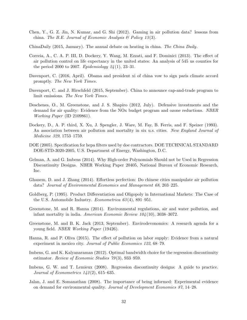
Chen, Y., G. Z. Jin, N. Kumar, and G. Shi (2012). Gaming in air pollution data? lessons fromchina. The B.E. Journal of Economic Analysis & Policy 13 (3).

ChinaDaily (2015, January). The annual debate on heating in china. The China Daily .

Correia, A., C. A. P. III, D. Dockery, Y. Wang, M. Ezzati, and F. Dominici (2013). The e↵ect ofair pollution control on life expectancy in the united states: An analysis of 545 us counties forthe period 2000 to 2007. Epidemiology 24 (1), 23–31.

Davenport, C. (2016, April). Obama and president xi of china vow to sign paris climate accordpromptly. The New York Times.

Davenport, C. and J. Hirschfeld (2015, September). China to announce cap-and-trade program tolimit emissions. The New York Times.

Deschenes, O., M. Greenstone, and J. S. Shapiro (2012, July). Defensive investments and thedemand for air quality: Evidence from the NOx budget program and ozone reductions. NBERWorking Paper (ID 2109861).

Dockery, D., A. P. third, X. Xu, J. Spengler, J. Ware, M. Fay, B. Ferris, and F. Speizer (1993).An association between air pollution and mortality in six u.s. cities. New England Journal ofMedicine 329, 1753–1759.

DOE (2005). Specification for hepa filters used by doe contractors. DOE TECHNICAL STANDARDDOE-STD-3020-2005, U.S. Department of Energy, Washington, D.C.

Gelman, A. and G. Imbens (2014). Why High-order Polynomials Should not be Used in RegressionDiscontinuity Designs. NBER Working Paper 20405, National Bureau of Economic Research,Inc.

Ghanem, D. and J. Zhang (2014). E↵ortless perfection: Do chinese cities manipulate air pollutiondata? Journal of Environmental Economics and Management 68, 203–225.

Goldberg, P. (1995). Product Di↵erentiation and Oligopoly in International Markets: The Case ofthe U.S. Automobile Industry. Econometrica 63 (4), 891–951.

Greenstone, M. and R. Hanna (2014). Environmental regulations, air and water pollution, andinfant mortality in india. American Economic Review 104 (10), 3038–3072.

Greenstone, M. and B. K. Jack (2013, September). Envirodevonomics: A research agenda for ayoung field. NBER Working Paper (19426).

Hanna, R. and P. Oliva (2015). The e↵ect of pollution on labor supply: Evidence from a naturalexperiment in mexico city. Journal of Public Economics 122, 68–79.

Imbens, G. and K. Kalyanaraman (2012). Optimal bandwidth choice for the regression discontinuityestimator. Review of Economic Studies 79 (3), 933–959.

Imbens, G. W. and T. Lemieux (2008). Regression discontinuity designs: A guide to practice.Journal of Econometrics 142 (2), 615–635.

Jalan, J. and E. Somanathan (2008). The importance of being informed: Experimental evidenceon demand for environmental quality. Journal of Development Economics 87, 14–28.

32

Jayachandran, S. (2009). Air quality and early-life mortality: Evidence from indonesia’s wildfires.Journal of Human Resources 44 (4), 916–954.

Knittel, C. R. and K. Metaxoglou (2013, May). Estimation of Random-Coe�cient Demand Models:Two Empiricists’ Perspective. Review of Economics and Statistics 96 (1), 34–59.

Kremer, M., J. Leino, E. Miguel, and A. P. Zwane (2011). Spring cleaning: Rural water impacts,valuation, and property rights institutions. The Quarterly Journal of Economics 126 (1), 145–205.

Lanphear, B., R. Hornung, J. Khoury, K. Yolton, M. Lierl, , and A. Kalkbrenner (2011). E↵ectsof hepa air cleaners on unscheduled asthma visits and asthma symptoms for children exposed tosecondhand tobacco smoke. Pediatrics 127 (1), 93–101.

Madajewicz, M., A. Pfa↵, A. van Geen, J. Graziano, I. Hussein, H. Momotaj, R. Sylvi, and H. Ahsan(2007). Can information alone change behavior? response to arsenic contamination of ground-water in bangladesh. Journal of Development Economics 84, 731–754.

McCrary, J. (2008). Manipulation of the running variable in the regression discontinuity design: Adensity test. Journal of Econometrics 142 (2), 698–714.

Miller, G. and M. Mobarak (2013). Gender di↵erences in preferences, intra-household externalities,and low demand for improved cookstoves. NBER Working Paper No.18964.

Mu, Q. and J. Zhang (2014). Air pollution and defensive expenditures: Evidence from particulate-filtering facemasks. E3 WP-078.

Neidell, M. (2009). Information, avoidance behavior, and health. Journal of Human Re-sources 44 (2), 450–478.

Nevo, A. (2001). Measuring market power in the ready-to-eat cereal industry. Econometrica 69 (2),307–342.

People’sDaily (2009, October). The vice minister of of the ministry of housing and urban-ruraldevelopment suggests three obstacles of implementing the heat reform. The People’s Daily .

Pope, C. A. I., M. Ezzati, and D. Dockery (2009). Fine-particulate air pollution and life expectancyin the united states. New England Journal of Medicine 360, 376–386.

Van Donkelaar, A., R. V. Martin, M. Brauer, R. Kahn, R. Levy, C. Verduzco, and P. J. Villeneuve(2010). Global estimates of ambient fine particulate matter concentrations from satellite-basedaerosol optical depth: Development and application. Environmental Health Perspectives 118 (6),847–855.

Wallace, L. (2008). E↵ectiveness of home air cleaners in reducing indoor levels of particles. Technicalreport, Health Canada.

Wong, E. (2014a, February). China to reward cities and regions making progress on air pollution.The New York Times.

Wong, E. (2014b, December). Fines total 26 million usd for polluters in china. The New YorkTimes.

Wong, E. (2015, December). China plans to upgrade coal plants. The New York Times.

33

WorldBank (2005). China - heat reform and building energy e�ciency project. Technical report,World Bank, Washington, DC.

WorldBank (2014). Implementation completion and results report on a global environment facilitygrant in the amount of usd 18 million to the people’s republic of china for a heat reform andbuilding energy e�ciency project. Technical Report ICR0003153, World Bank, Washington, D.C.

Zhang, X. (2015, April). Indoor air pollution in beijing. The People’s Daily .

Zheng, S., C. Sun, and M. Kahn (2015). Self-protection investment exacerbates air pollutionexposure inequality in urban china. NBER Working Paper No.21301.

Zhu, N. (2014, March). Xinhua insight: China declares war against pollution. Xinhua News Agency .

Zivin, J. G. and M. Neidell (2009). Days of haze: Environmental information disclosure andintertemporal avoidance behavior. Journal of Environmental Economics and Management 58,119–128.

Zivin, J. G., M. Neidell, and W. Schlenker (2011). Water quality violations and avoidance be-havior: Evidence from bottled water consumption. American Economic Review: Papers andProceedings 101 (3), 448–453.

34

Figure 1: Huai River Boundary and City Locations

Notes: The line in the middle of the map is the Huai River-Qinling boundary. Each dot represents one city.There are 81 cities in our sample.

35

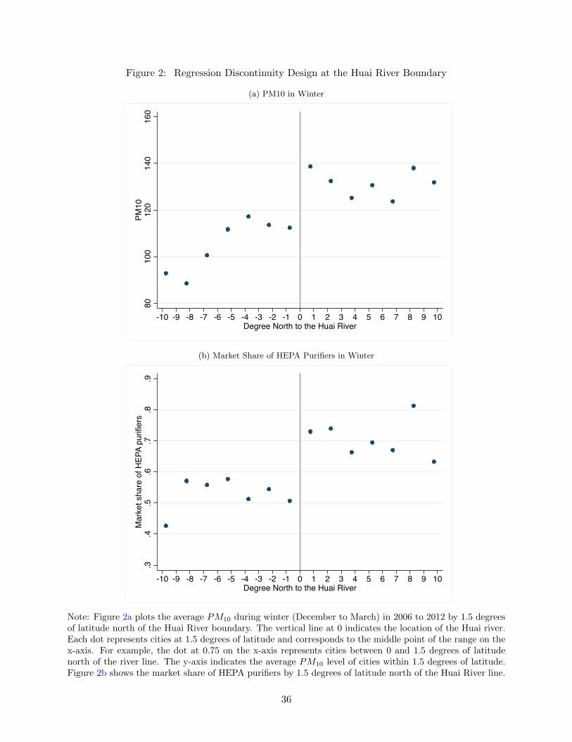
Figure 2: Regression Discontinuity Design at the Huai River Boundary

(a) PM10 in Winter

8010

012

014

016

0PM

10

-10 -9 -8 -7 -6 -5 -4 -3 -2 -1 0 1 2 3 4 5 6 7 8 9 10Degree North to the Huai River

(b) Market Share of HEPA Purifiers in Winter

.3.4

.5.6

.7.8

.9M

arke

t sha

re o

f HEP

A pu

rifier

s

-10 -9 -8 -7 -6 -5 -4 -3 -2 -1 0 1 2 3 4 5 6 7 8 9 10Degree North to the Huai River

Note: Figure 2a plots the average PM10 during winter (December to March) in 2006 to 2012 by 1.5 degreesof latitude north of the Huai River boundary. The vertical line at 0 indicates the location of the Huai river.Each dot represents cities at 1.5 degrees of latitude and corresponds to the middle point of the range on thex-axis. For example, the dot at 0.75 on the x-axis represents cities between 0 and 1.5 degrees of latitudenorth of the river line. The y-axis indicates the average PM10 level of cities within 1.5 degrees of latitude.Figure 2b shows the market share of HEPA purifiers by 1.5 degrees of latitude north of the Huai River line.

36

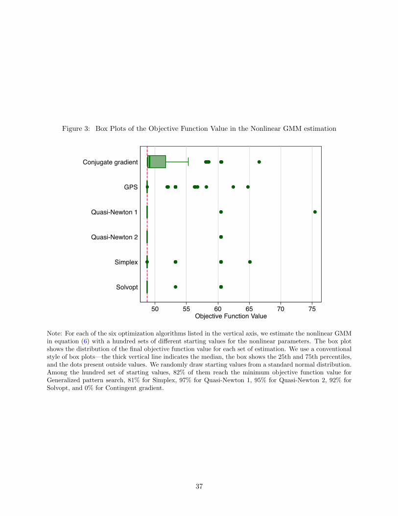
Figure 3: Box Plots of the Objective Function Value in the Nonlinear GMM estimation

50 55 60 65 70 75Objective Function Value

Solvopt

Simplex

Quasi-Newton 2

Quasi-Newton 1

GPS

Conjugate gradient

Note: For each of the six optimization algorithms listed in the vertical axis, we estimate the nonlinear GMMin equation (6) with a hundred sets of di↵erent starting values for the nonlinear parameters. The box plotshows the distribution of the final objective function value for each set of estimation. We use a conventionalstyle of box plots—the thick vertical line indicates the median, the box shows the 25th and 75th percentiles,and the dots present outside values. We randomly draw starting values from a standard normal distribution.Among the hundred set of starting values, 82% of them reach the minimum objective function value forGeneralized pattern search, 81% for Simplex, 97% for Quasi-Newton 1, 95% for Quasi-Newton 2, 92% forSolvopt, and 0% for Contingent gradient.

37

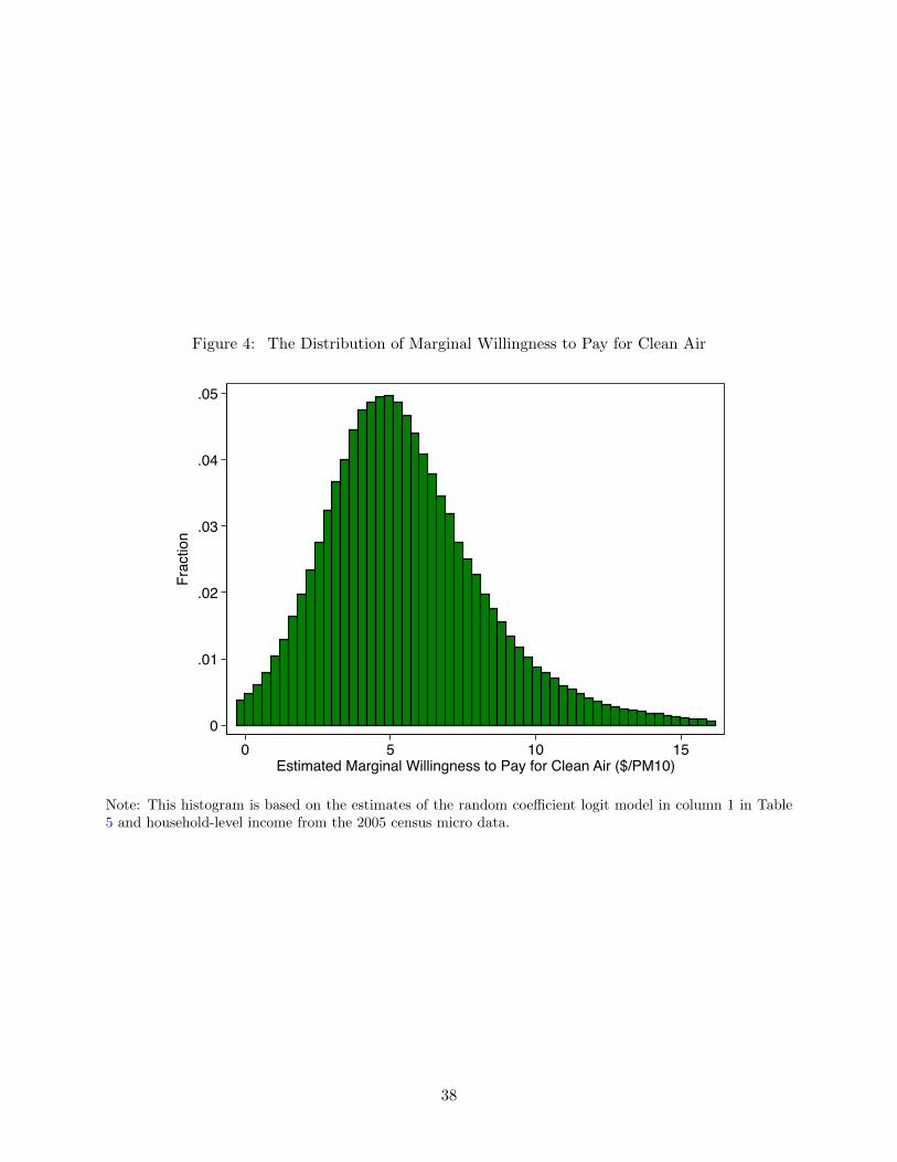
Figure 4: The Distribution of Marginal Willingness to Pay for Clean Air

0

.01

.02

.03

.04

.05

Frac

tion

0 5 10 15Estimated Marginal Willingness to Pay for Clean Air ($/PM10)

Note: This histogram is based on the estimates of the random coe�cient logit model in column 1 in Table5 and household-level income from the 2005 census micro data.

38

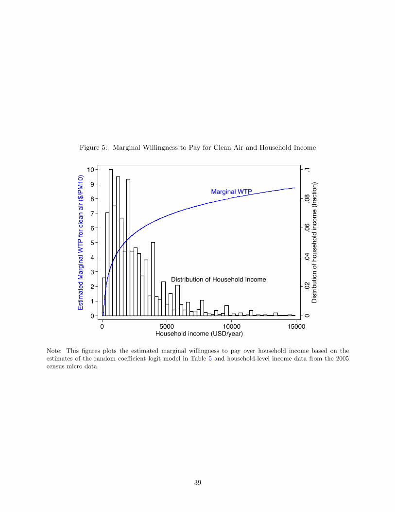
Figure 5: Marginal Willingness to Pay for Clean Air and Household Income

Marginal WTP

Distribution of Household Income

0.0

2.0

4.0

6.0

8.1

Dis

tribu

tion

of h

ouse

hold

inco

me

(frac

tion)

0

1

2

3

4

5

6

7

8

9

10

Estim

ated

Mar

gina

l WTP

for c

lean

air

($/P

M10

)

0 5000 10000 15000Household income (USD/year)

Note: This figures plots the estimated marginal willingness to pay over household income based on theestimates of the random coe�cient logit model in Table 5 and household-level income data from the 2005census micro data.

39

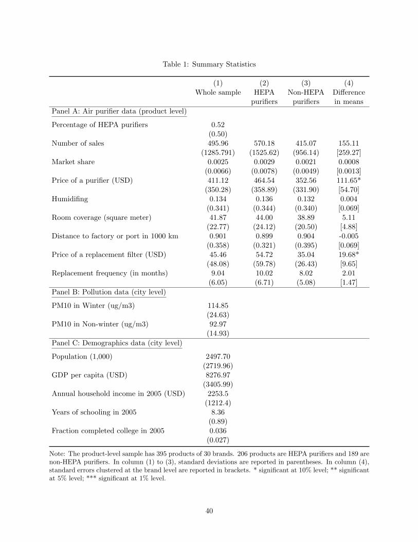
Table 1: Summary Statistics

(1) (2) (3) (4)Whole sample HEPA Non-HEPA Di↵erence

purifiers purifiers in meansPanel A: Air purifier data (product level)

Percentage of HEPA purifiers 0.52(0.50)

Number of sales 495.96 570.18 415.07 155.11(1285.791) (1525.62) (956.14) [259.27]

Market share 0.0025 0.0029 0.0021 0.0008(0.0066) (0.0078) (0.0049) [0.0013]

Price of a purifier (USD) 411.12 464.54 352.56 111.65*(350.28) (358.89) (331.90) [54.70]

Humidifing 0.134 0.136 0.132 0.004(0.341) (0.344) (0.340) [0.069]

Room coverage (square meter) 41.87 44.00 38.89 5.11(22.77) (24.12) (20.50) [4.88]

Distance to factory or port in 1000 km 0.901 0.899 0.904 -0.005(0.358) (0.321) (0.395) [0.069]

Price of a replacement filter (USD) 45.46 54.72 35.04 19.68*(48.08) (59.78) (26.43) [9.65]

Replacement frequency (in months) 9.04 10.02 8.02 2.01(6.05) (6.71) (5.08) [1.47]

Panel B: Pollution data (city level)

PM10 in Winter (ug/m3) 114.85(24.63)

PM10 in Non-winter (ug/m3) 92.97(14.93)

Panel C: Demographics data (city level)

Population (1,000) 2497.70(2719.96)

GDP per capita (USD) 8276.97(3405.99)

Annual household income in 2005 (USD) 2253.5(1212.4)

Years of schooling in 2005 8.36(0.89)

Fraction completed college in 2005 0.036(0.027)

Note: The product-level sample has 395 products of 30 brands. 206 products are HEPA purifiers and 189 arenon-HEPA purifiers. In column (1) to (3), standard deviations are reported in parentheses. In column (4),standard errors clustered at the brand level are reported in brackets. * significant at 10% level; ** significantat 5% level; *** significant at 1% level.

40

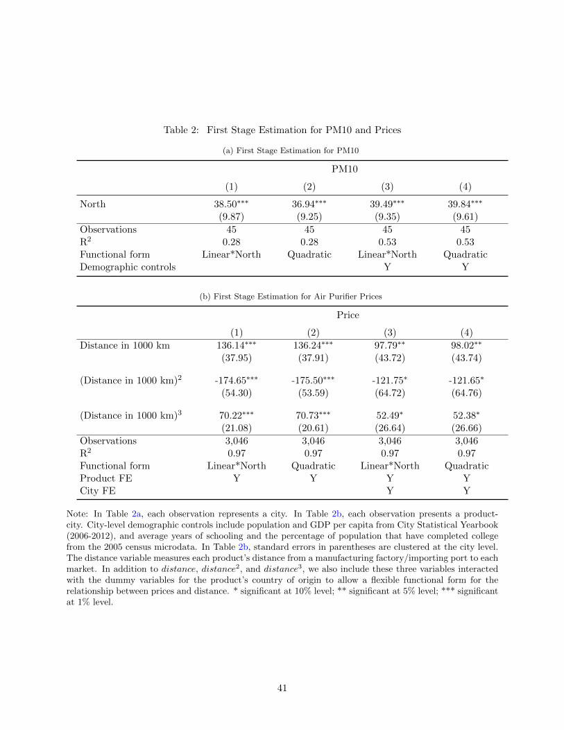
Table 2: First Stage Estimation for PM10 and Prices

(a) First Stage Estimation for PM10

PM10

(1) (2) (3) (4)

North 38.50⇤⇤⇤ 36.94⇤⇤⇤ 39.49⇤⇤⇤ 39.84⇤⇤⇤

(9.87) (9.25) (9.35) (9.61)Observations 45 45 45 45R2 0.28 0.28 0.53 0.53Functional form Linear*North Quadratic Linear*North QuadraticDemographic controls Y Y

(b) First Stage Estimation for Air Purifier Prices

Price

(1) (2) (3) (4)Distance in 1000 km 136.14⇤⇤⇤ 136.24⇤⇤⇤ 97.79⇤⇤ 98.02⇤⇤

(37.95) (37.91) (43.72) (43.74)

(Distance in 1000 km)2 -174.65⇤⇤⇤ -175.50⇤⇤⇤ -121.75⇤ -121.65⇤

(54.30) (53.59) (64.72) (64.76)

(Distance in 1000 km)3 70.22⇤⇤⇤ 70.73⇤⇤⇤ 52.49⇤ 52.38⇤

(21.08) (20.61) (26.64) (26.66)Observations 3,046 3,046 3,046 3,046R2 0.97 0.97 0.97 0.97Functional form Linear*North Quadratic Linear*North QuadraticProduct FE Y Y Y YCity FE Y Y

Note: In Table 2a, each observation represents a city. In Table 2b, each observation presents a product-city. City-level demographic controls include population and GDP per capita from City Statistical Yearbook(2006-2012), and average years of schooling and the percentage of population that have completed collegefrom the 2005 census microdata. In Table 2b, standard errors in parentheses are clustered at the city level.The distance variable measures each product’s distance from a manufacturing factory/importing port to eachmarket. In addition to distance, distance2, and distance3, we also include these three variables interactedwith the dummy variables for the product’s country of origin to allow a flexible functional form for therelationship between prices and distance. * significant at 10% level; ** significant at 5% level; *** significantat 1% level.

41

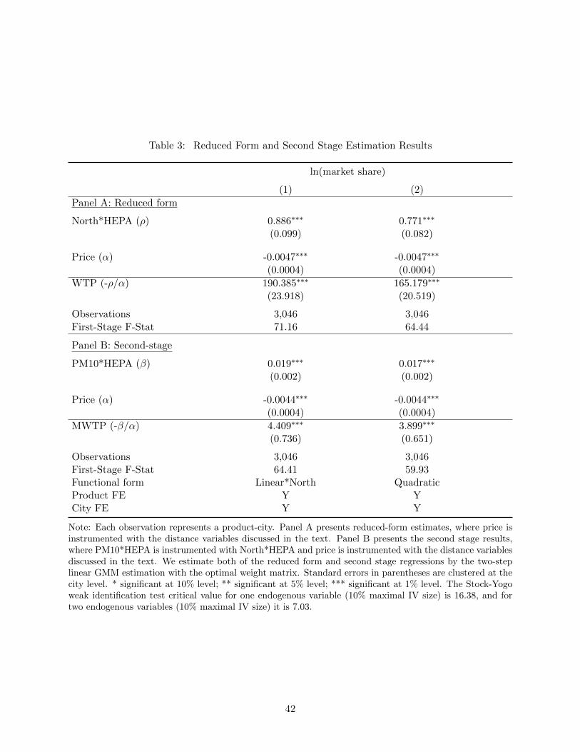
Table 3: Reduced Form and Second Stage Estimation Results

ln(market share)

(1) (2)Panel A: Reduced form

North*HEPA (⇢) 0.886⇤⇤⇤ 0.771⇤⇤⇤

(0.099) (0.082)

Price (↵) -0.0047⇤⇤⇤ -0.0047⇤⇤⇤

(0.0004) (0.0004)WTP (-⇢/↵) 190.385⇤⇤⇤ 165.179⇤⇤⇤

(23.918) (20.519)

Observations 3,046 3,046First-Stage F-Stat 71.16 64.44

Panel B: Second-stage

PM10*HEPA (�) 0.019⇤⇤⇤ 0.017⇤⇤⇤

(0.002) (0.002)

Price (↵) -0.0044⇤⇤⇤ -0.0044⇤⇤⇤

(0.0004) (0.0004)MWTP (-�/↵) 4.409⇤⇤⇤ 3.899⇤⇤⇤

(0.736) (0.651)

Observations 3,046 3,046First-Stage F-Stat 64.41 59.93Functional form Linear*North QuadraticProduct FE Y YCity FE Y Y

Note: Each observation represents a product-city. Panel A presents reduced-form estimates, where price isinstrumented with the distance variables discussed in the text. Panel B presents the second stage results,where PM10*HEPA is instrumented with North*HEPA and price is instrumented with the distance variablesdiscussed in the text. We estimate both of the reduced form and second stage regressions by the two-steplinear GMM estimation with the optimal weight matrix. Standard errors in parentheses are clustered at thecity level. * significant at 10% level; ** significant at 5% level; *** significant at 1% level. The Stock-Yogoweak identification test critical value for one endogenous variable (10% maximal IV size) is 16.38, and fortwo endogenous variables (10% maximal IV size) it is 7.03.

42

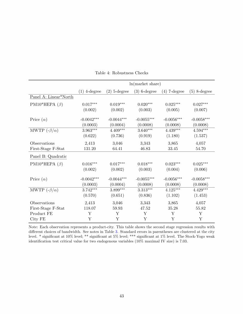
Table 4: Robustness Checks

ln(market share)

(1) 4-degree (2) 5-degree (3) 6-degree (4) 7-degree (5) 8-degreePanel A: Linear*North

PM10*HEPA (�) 0.017⇤⇤⇤ 0.019⇤⇤⇤ 0.020⇤⇤⇤ 0.025⇤⇤⇤ 0.027⇤⇤⇤

(0.002) (0.002) (0.003) (0.005) (0.007)

Price (↵) -0.0042⇤⇤⇤ -0.0044⇤⇤⇤ -0.0055⇤⇤⇤ -0.0056⇤⇤⇤ -0.0058⇤⇤⇤

(0.0003) (0.0004) (0.0008) (0.0008) (0.0008)MWTP (-�/↵) 3.963⇤⇤⇤ 4.409⇤⇤⇤ 3.640⇤⇤⇤ 4.439⇤⇤⇤ 4.594⇤⇤⇤

(0.622) (0.736) (0.919) (1.180) (1.537)

Observations 2,413 3,046 3,343 3,865 4,057First-Stage F-Stat 131.20 64.41 46.83 33.45 54.70

Panel B: Quadratic

PM10*HEPA (�) 0.016⇤⇤⇤ 0.017⇤⇤⇤ 0.018⇤⇤⇤ 0.023⇤⇤⇤ 0.025⇤⇤⇤

(0.002) (0.002) (0.003) (0.004) (0.006)

Price (↵) -0.0042⇤⇤⇤ -0.0044⇤⇤⇤ -0.0055⇤⇤⇤ -0.0056⇤⇤⇤ -0.0058⇤⇤⇤

(0.0003) (0.0004) (0.0008) (0.0008) (0.0008)MWTP (-�/↵) 3.742⇤⇤⇤ 3.899⇤⇤⇤ 3.313⇤⇤⇤ 4.125⇤⇤⇤ 4.429⇤⇤⇤

(0.570) (0.651) (0.836) (1.102) (1.453)

Observations 2,413 3,046 3,343 3,865 4,057First-Stage F-Stat 118.07 59.93 47.52 35.28 55.82Product FE Y Y Y Y YCity FE Y Y Y Y Y

Note: Each observation represents a product-city. This table shows the second stage regression results withdi↵erent choices of bandwidth. See notes in Table 3. Standard errors in parentheses are clustered at the citylevel. * significant at 10% level; ** significant at 5% level; *** significant at 1% level. The Stock-Yogo weakidentification test critical value for two endogenous variables (10% maximal IV size) is 7.03.

43

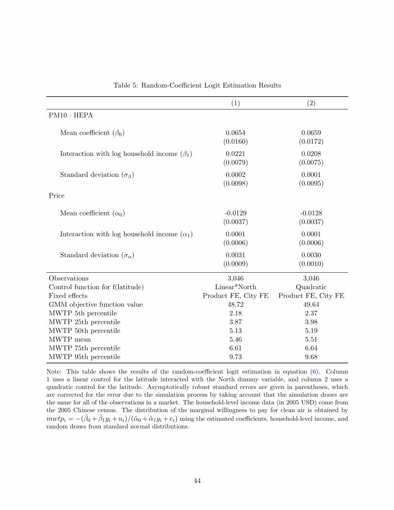
Table 5: Random-Coe�cient Logit Estimation Results

(1) (2)

PM10 · HEPA

Mean coe�cient (�0) 0.0654 0.0659(0.0160) (0.0172)

Interaction with log household income (�1) 0.0221 0.0208(0.0079) (0.0075)

Standard deviation (��) 0.0002 0.0001(0.0098) (0.0095)

Price

Mean coe�cient (↵0) -0.0129 -0.0128(0.0037) (0.0037)

Interaction with log household income (↵1) 0.0001 0.0001(0.0006) (0.0006)

Standard deviation (�↵) 0.0031 0.0030(0.0009) (0.0010)

Observations 3,046 3,046Control function for f(latitude) Linear*North QuadraticFixed e↵ects Product FE, City FE Product FE, City FEGMM objective function value 48.72 49.64MWTP 5th percentile 2.18 2.37MWTP 25th percentile 3.87 3.98MWTP 50th percentile 5.13 5.19MWTP mean 5.46 5.51MWTP 75th percentile 6.61 6.64MWTP 95th percentile 9.73 9.68

Note: This table shows the results of the random-coe�cient logit estimation in equation (6). Column1 uses a linear control for the latitude interacted with the North dummy variable, and column 2 uses aquadratic control for the latitude. Asymptotically robust standard errors are given in parentheses, whichare corrected for the error due to the simulation process by taking account that the simulation draws arethe same for all of the observations in a market. The household-level income data (in 2005 USD) come fromthe 2005 Chinese census. The distribution of the marginal willingness to pay for clean air is obtained by

mwtpi = �(�̂0+ �̂1yi+ui)/(↵̂0+ ↵̂1yi+ ei) using the estimated coe�cients, household-level income, andrandom draws from standard normal distributions.

44

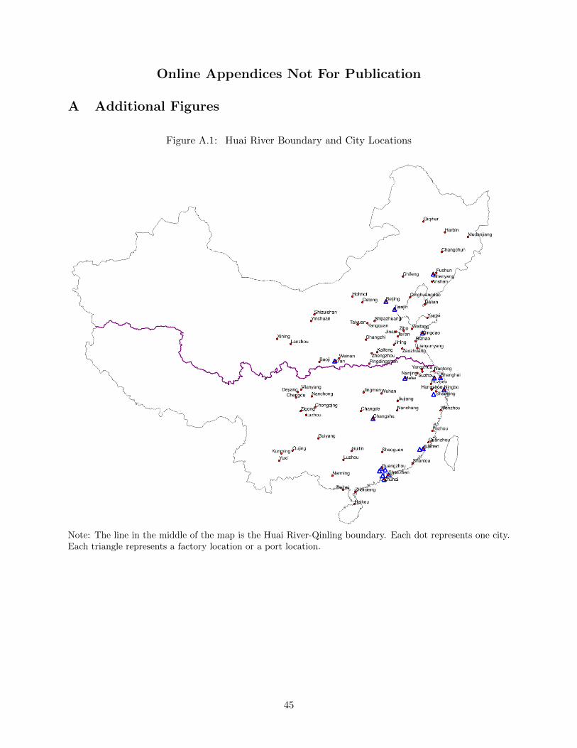
Online Appendices Not For Publication

A Additional Figures

Figure A.1: Huai River Boundary and City Locations

Note: The line in the middle of the map is the Huai River-Qinling boundary. Each dot represents one city.Each triangle represents a factory location or a port location.

45

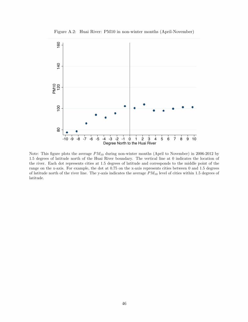
Figure A.2: Huai River: PM10 in non-winter months (April-November)

8010

012

014

016

0PM

10

-10 -9 -8 -7 -6 -5 -4 -3 -2 -1 0 1 2 3 4 5 6 7 8 9 10Degree North to the Huai River

Note: This figure plots the average PM10 during non-winter months (April to November) in 2006-2012 by1.5 degrees of latitude north of the Huai River boundary. The vertical line at 0 indicates the location ofthe river. Each dot represents cities at 1.5 degrees of latitude and corresponds to the middle point of therange on the x-axis. For example, the dot at 0.75 on the x-axis represents cities between 0 and 1.5 degreesof latitude north of the river line. The y-axis indicates the average PM10 level of cities within 1.5 degrees oflatitude.

46

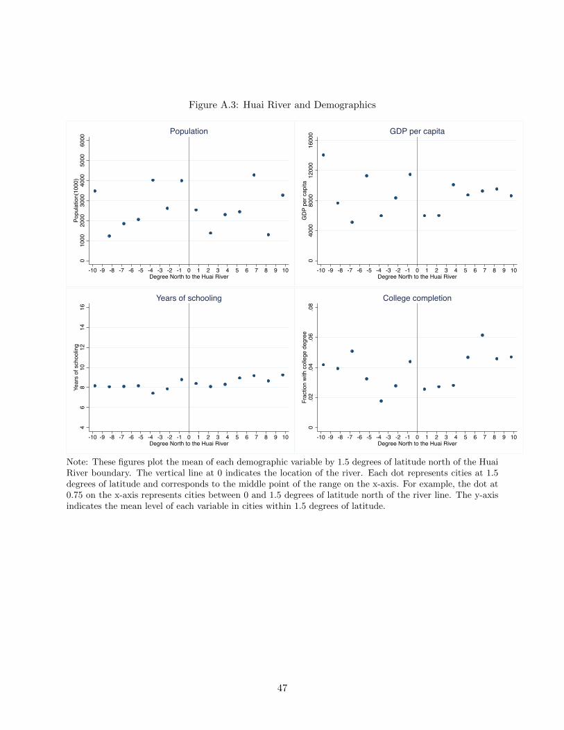
Figure A.3: Huai River and Demographics

010

0020

0030

0040

0050

0060

00Po

pula

tion(

1000

)

-10 -9 -8 -7 -6 -5 -4 -3 -2 -1 0 1 2 3 4 5 6 7 8 9 10Degree North to the Huai River

Population

040

0080

0012

000

1600

0G

DP

per c

apita

-10 -9 -8 -7 -6 -5 -4 -3 -2 -1 0 1 2 3 4 5 6 7 8 9 10Degree North to the Huai River

GDP per capita

46

810

1214

16Ye

ars

of s

choo

ling

-10 -9 -8 -7 -6 -5 -4 -3 -2 -1 0 1 2 3 4 5 6 7 8 9 10Degree North to the Huai River

Years of schooling0

.02

.04

.06

.08

Frac

tion

with

col

lege

deg

ree

-10 -9 -8 -7 -6 -5 -4 -3 -2 -1 0 1 2 3 4 5 6 7 8 9 10Degree North to the Huai River

College completion

Note: These figures plot the mean of each demographic variable by 1.5 degrees of latitude north of the HuaiRiver boundary. The vertical line at 0 indicates the location of the river. Each dot represents cities at 1.5degrees of latitude and corresponds to the middle point of the range on the x-axis. For example, the dot at0.75 on the x-axis represents cities between 0 and 1.5 degrees of latitude north of the river line. The y-axisindicates the mean level of each variable in cities within 1.5 degrees of latitude.

47

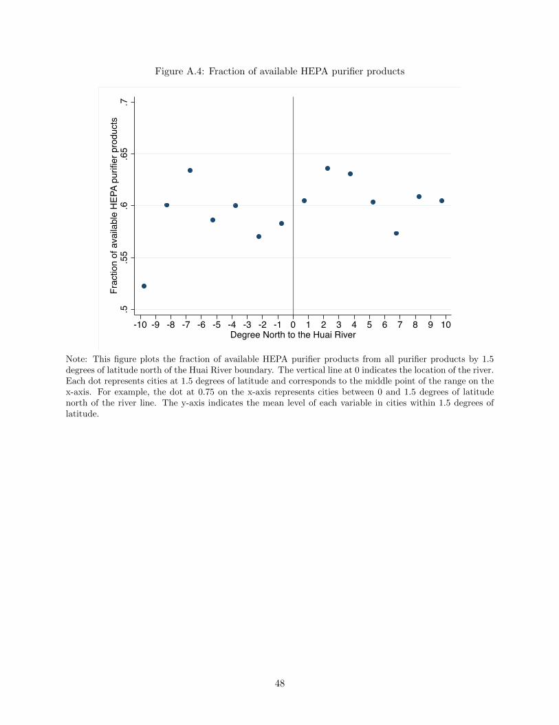
Figure A.4: Fraction of available HEPA purifier products

.5.5

5.6

.65

.7Fr

actio

n of

ava

ilabl

e H

EPA

purifi

er p

rodu

cts

-10 -9 -8 -7 -6 -5 -4 -3 -2 -1 0 1 2 3 4 5 6 7 8 9 10Degree North to the Huai River

Note: This figure plots the fraction of available HEPA purifier products from all purifier products by 1.5degrees of latitude north of the Huai River boundary. The vertical line at 0 indicates the location of the river.Each dot represents cities at 1.5 degrees of latitude and corresponds to the middle point of the range on thex-axis. For example, the dot at 0.75 on the x-axis represents cities between 0 and 1.5 degrees of latitudenorth of the river line. The y-axis indicates the mean level of each variable in cities within 1.5 degrees oflatitude.

48

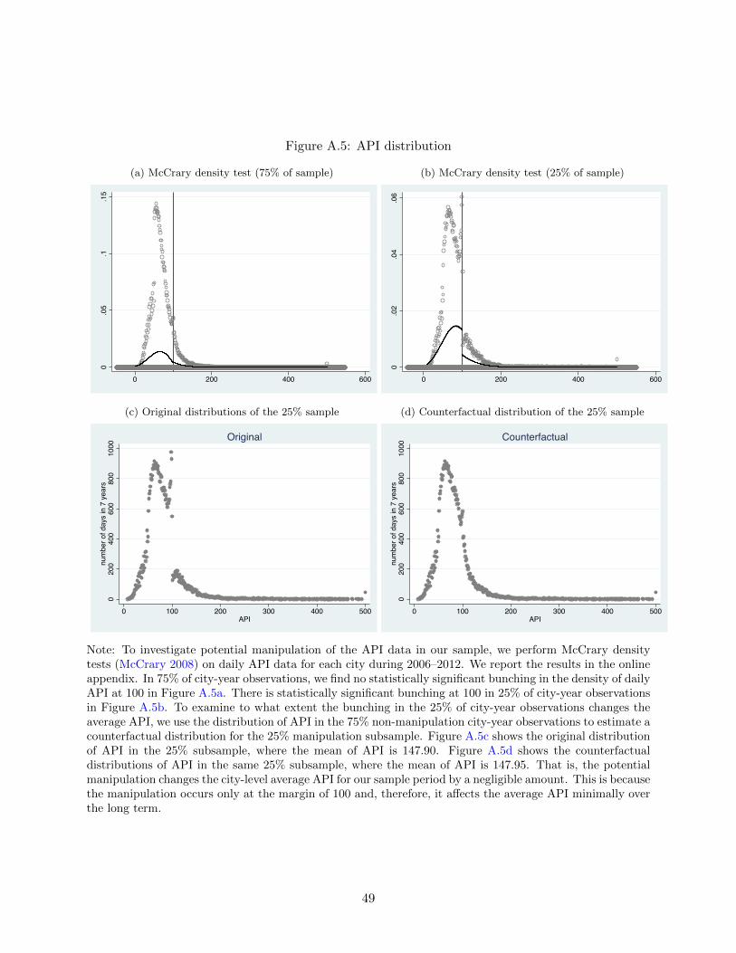
Figure A.5: API distribution

(a) McCrary density test (75% of sample)

0.05

.1.15

0 200 400 600

(b) McCrary density test (25% of sample)

0.02

.04

.06

0 200 400 600

(c) Original distributions of the 25% sample

020

040

060

080

010

00nu

mbe

r of d

ays

in 7

yea

rs

0 100 200 300 400 500API

Original

(d) Counterfactual distribution of the 25% sample0

200

400

600

800

1000

num

ber o

f day

s in

7 y

ears

0 100 200 300 400 500API

Counterfactual

Note: To investigate potential manipulation of the API data in our sample, we perform McCrary densitytests (McCrary 2008) on daily API data for each city during 2006–2012. We report the results in the onlineappendix. In 75% of city-year observations, we find no statistically significant bunching in the density of dailyAPI at 100 in Figure A.5a. There is statistically significant bunching at 100 in 25% of city-year observationsin Figure A.5b. To examine to what extent the bunching in the 25% of city-year observations changes theaverage API, we use the distribution of API in the 75% non-manipulation city-year observations to estimate acounterfactual distribution for the 25% manipulation subsample. Figure A.5c shows the original distributionof API in the 25% subsample, where the mean of API is 147.90. Figure A.5d shows the counterfactualdistributions of API in the same 25% subsample, where the mean of API is 147.95. That is, the potentialmanipulation changes the city-level average API for our sample period by a negligible amount. This is becausethe manipulation occurs only at the margin of 100 and, therefore, it a↵ects the average API minimally overthe long term.

49

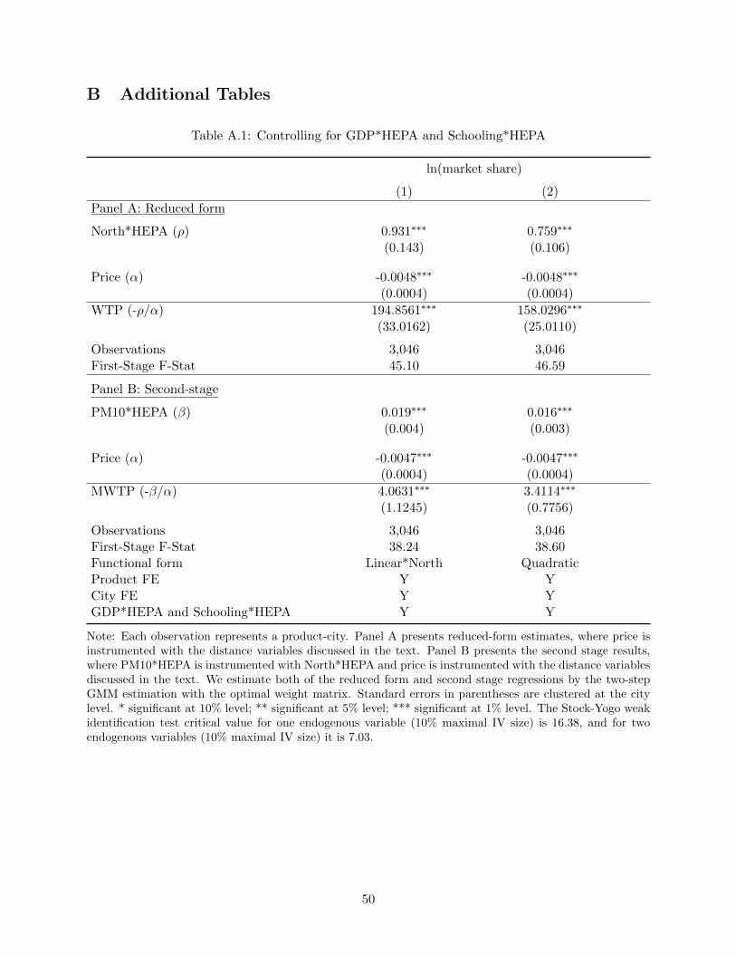
B Additional Tables

Table A.1: Controlling for GDP*HEPA and Schooling*HEPA

ln(market share)

(1) (2)Panel A: Reduced form

North*HEPA (⇢) 0.931⇤⇤⇤ 0.759⇤⇤⇤

(0.143) (0.106)

Price (↵) -0.0048⇤⇤⇤ -0.0048⇤⇤⇤

(0.0004) (0.0004)WTP (-⇢/↵) 194.8561⇤⇤⇤ 158.0296⇤⇤⇤

(33.0162) (25.0110)

Observations 3,046 3,046First-Stage F-Stat 45.10 46.59

Panel B: Second-stage

PM10*HEPA (�) 0.019⇤⇤⇤ 0.016⇤⇤⇤

(0.004) (0.003)

Price (↵) -0.0047⇤⇤⇤ -0.0047⇤⇤⇤

(0.0004) (0.0004)MWTP (-�/↵) 4.0631⇤⇤⇤ 3.4114⇤⇤⇤

(1.1245) (0.7756)

Observations 3,046 3,046First-Stage F-Stat 38.24 38.60Functional form Linear*North QuadraticProduct FE Y YCity FE Y YGDP*HEPA and Schooling*HEPA Y Y

Note: Each observation represents a product-city. Panel A presents reduced-form estimates, where price isinstrumented with the distance variables discussed in the text. Panel B presents the second stage results,where PM10*HEPA is instrumented with North*HEPA and price is instrumented with the distance variablesdiscussed in the text. We estimate both of the reduced form and second stage regressions by the two-stepGMM estimation with the optimal weight matrix. Standard errors in parentheses are clustered at the citylevel. * significant at 10% level; ** significant at 5% level; *** significant at 1% level. The Stock-Yogo weakidentification test critical value for one endogenous variable (10% maximal IV size) is 16.38, and for twoendogenous variables (10% maximal IV size) it is 7.03.

50

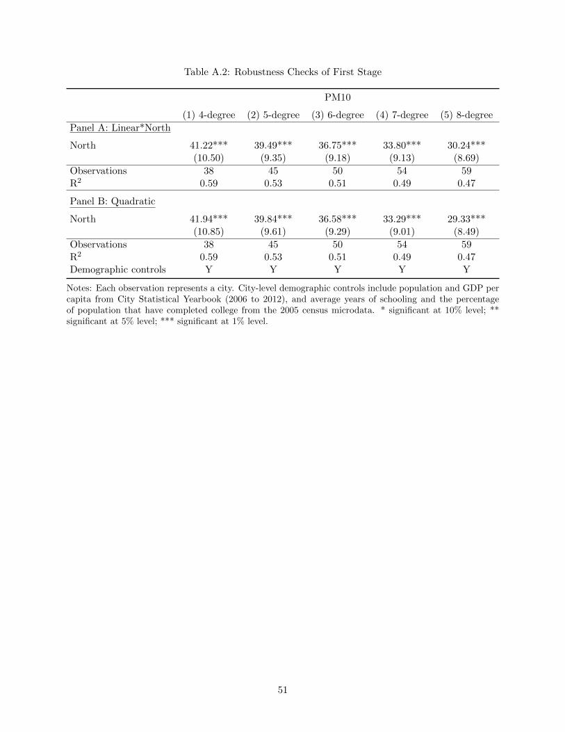
Table A.2: Robustness Checks of First Stage

PM10

(1) 4-degree (2) 5-degree (3) 6-degree (4) 7-degree (5) 8-degreePanel A: Linear*North

North 41.22*** 39.49*** 36.75*** 33.80*** 30.24***(10.50) (9.35) (9.18) (9.13) (8.69)

Observations 38 45 50 54 59R2 0.59 0.53 0.51 0.49 0.47

Panel B: Quadratic

North 41.94*** 39.84*** 36.58*** 33.29*** 29.33***(10.85) (9.61) (9.29) (9.01) (8.49)

Observations 38 45 50 54 59R2 0.59 0.53 0.51 0.49 0.47Demographic controls Y Y Y Y Y

Notes: Each observation represents a city. City-level demographic controls include population and GDP percapita from City Statistical Yearbook (2006 to 2012), and average years of schooling and the percentageof population that have completed college from the 2005 census microdata. * significant at 10% level; **significant at 5% level; *** significant at 1% level.

51

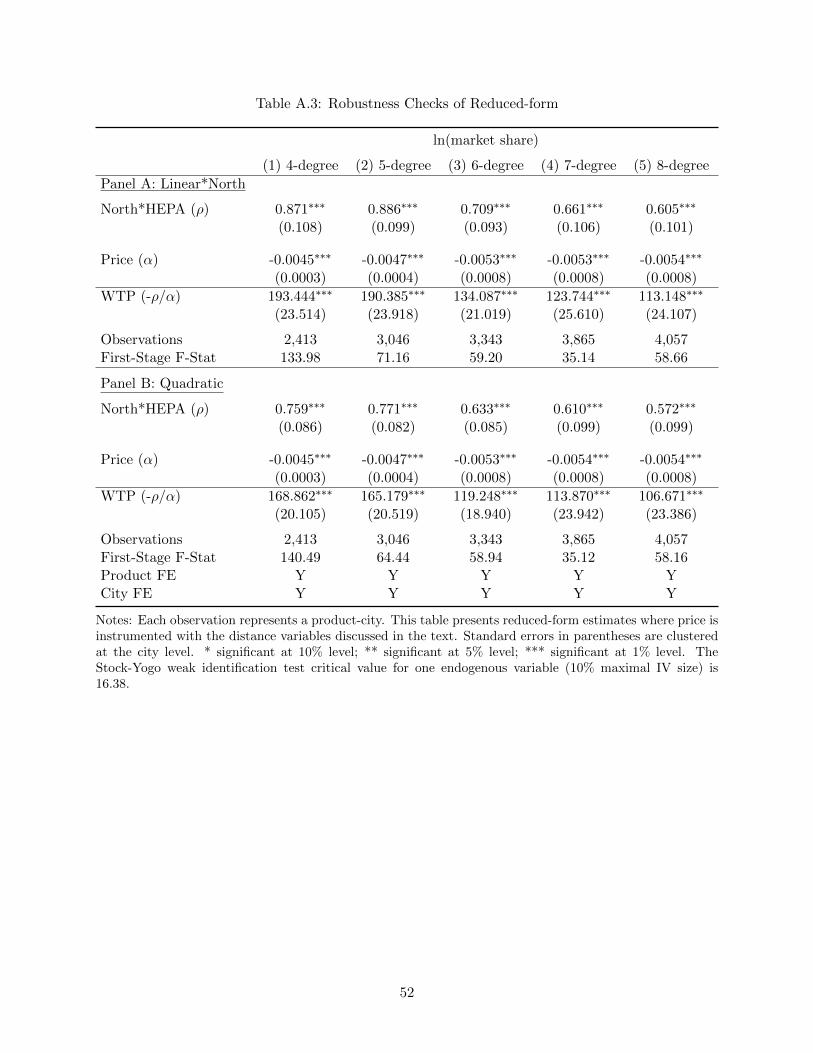
Table A.3: Robustness Checks of Reduced-form

ln(market share)

(1) 4-degree (2) 5-degree (3) 6-degree (4) 7-degree (5) 8-degreePanel A: Linear*North

North*HEPA (⇢) 0.871⇤⇤⇤ 0.886⇤⇤⇤ 0.709⇤⇤⇤ 0.661⇤⇤⇤ 0.605⇤⇤⇤

(0.108) (0.099) (0.093) (0.106) (0.101)

Price (↵) -0.0045⇤⇤⇤ -0.0047⇤⇤⇤ -0.0053⇤⇤⇤ -0.0053⇤⇤⇤ -0.0054⇤⇤⇤

(0.0003) (0.0004) (0.0008) (0.0008) (0.0008)WTP (-⇢/↵) 193.444⇤⇤⇤ 190.385⇤⇤⇤ 134.087⇤⇤⇤ 123.744⇤⇤⇤ 113.148⇤⇤⇤

(23.514) (23.918) (21.019) (25.610) (24.107)

Observations 2,413 3,046 3,343 3,865 4,057First-Stage F-Stat 133.98 71.16 59.20 35.14 58.66

Panel B: Quadratic

North*HEPA (⇢) 0.759⇤⇤⇤ 0.771⇤⇤⇤ 0.633⇤⇤⇤ 0.610⇤⇤⇤ 0.572⇤⇤⇤

(0.086) (0.082) (0.085) (0.099) (0.099)

Price (↵) -0.0045⇤⇤⇤ -0.0047⇤⇤⇤ -0.0053⇤⇤⇤ -0.0054⇤⇤⇤ -0.0054⇤⇤⇤

(0.0003) (0.0004) (0.0008) (0.0008) (0.0008)WTP (-⇢/↵) 168.862⇤⇤⇤ 165.179⇤⇤⇤ 119.248⇤⇤⇤ 113.870⇤⇤⇤ 106.671⇤⇤⇤

(20.105) (20.519) (18.940) (23.942) (23.386)

Observations 2,413 3,046 3,343 3,865 4,057First-Stage F-Stat 140.49 64.44 58.94 35.12 58.16Product FE Y Y Y Y YCity FE Y Y Y Y Y

Notes: Each observation represents a product-city. This table presents reduced-form estimates where price isinstrumented with the distance variables discussed in the text. Standard errors in parentheses are clusteredat the city level. * significant at 10% level; ** significant at 5% level; *** significant at 1% level. TheStock-Yogo weak identification test critical value for one endogenous variable (10% maximal IV size) is16.38.

52

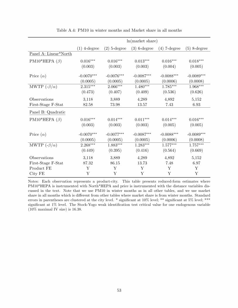
Table A.4: PM10 in winter months and Market share in all months

ln(market share)

(1) 4-degree (2) 5-degree (3) 6-degree (4) 7-degree (5) 8-degreePanel A: Linear*North

PM10*HEPA (�) 0.016⇤⇤⇤ 0.016⇤⇤⇤ 0.013⇤⇤⇤ 0.016⇤⇤⇤ 0.018⇤⇤⇤

(0.003) (0.003) (0.003) (0.004) (0.005)

Price (↵) -0.0070⇤⇤⇤ -0.0076⇤⇤⇤ -0.0087⇤⇤⇤ -0.0088⇤⇤⇤ -0.0089⇤⇤⇤

(0.0005) (0.0005) (0.0005) (0.0006) (0.0008)MWTP (-�/↵) 2.315⇤⇤⇤ 2.066⇤⇤⇤ 1.480⇤⇤⇤ 1.785⇤⇤⇤ 1.968⇤⇤⇤

(0.473) (0.407) (0.409) (0.536) (0.626)

Observations 3,118 3,889 4,289 4,892 5,152First-Stage F-Stat 82.58 73.98 13.57 7.43 6.93

Panel B: Quadratic

PM10*HEPA (�) 0.016⇤⇤⇤ 0.014⇤⇤⇤ 0.011⇤⇤⇤ 0.014⇤⇤⇤ 0.016⇤⇤⇤

(0.003) (0.003) (0.003) (0.005) (0.005)

Price (↵) -0.0070⇤⇤⇤ -0.0077⇤⇤⇤ -0.0087⇤⇤⇤ -0.0088⇤⇤⇤ -0.0089⇤⇤⇤

(0.0005) (0.0005) (0.0005) (0.0006) (0.0008)MWTP (-�/↵) 2.268⇤⇤⇤ 1.883⇤⇤⇤ 1.283⇤⇤⇤ 1.577⇤⇤⇤ 1.757⇤⇤⇤

(0.449) (0.395) (0.416) (0.564) (0.669)

Observations 3,118 3,889 4,289 4,892 5,152First-Stage F-Stat 87.32 86.15 13.73 7.48 6.97Product FE Y Y Y Y YCity FE Y Y Y Y Y

Notes: Each observation represents a product-city. This table presents reduced-form estimates wherePM10*HEPA is instrumented with North*HEPA and price is instrumented with the distance variables dis-cussed in the text. Note that we use PM10 in winter months as in all other tables, and we use marketshare in all months which is di↵erent from other tables where market share is from winter months. Standarderrors in parentheses are clustered at the city level. * significant at 10% level; ** significant at 5% level; ***significant at 1% level. The Stock-Yogo weak identification test critical value for one endogenous variable(10% maximal IV size) is 16.38.

53