CHAPTER 10

WILDFIRE AND THE ECONOMIC VALUE OF WILDERNESS RECREATION

Jeffrey Englin, Thomas P. Holmes, and Janet Lutz

1. INTRODUCTION

The idea that wildfires play an integral role in maintaining healthy forests has begun to change the ways that scientists, managers, and the general public view fire policy and programs. New approaches to forest management that seek to integrate natural disturbances with the provision of goods and services valued by people impose a greater need for a full accounting of the economic effects of wild­fire (as well as other disturbances). In addition to the effects that forest fires have on commodities and assets that are traded in markets, such as timber and residen­tial structures, fires also affect the condition and value of public goods that are not traded in markets, such as outdoor recreational sites. Understanding the economic consequences of wildfires on the provision and value of public goods requires the use of non-market valuation methods (Champ et al. 2003). The goal of this chapter is to demonstrate how wildfires affect the demand for, and value of, Wilderness recreational sites, which is illustrated using the travel cost method.1

Wilderness areas provide the public with a special opportunity to observe the effects of wildfires on natural processes in fire-adapted ecosystems. Lightning­caused fires are sometimes allowed to bum in Wilderness areas (a prescribed natural fire) when conditions are deemed suitable. Management ignited prescribed fires are also used to reduce fuel loads and mimic natural processes (Geary and Stokes 1999). Although fire suppression activities are permitted in Wilderness areas, management of forest regeneration and succession after a wild­fire (including timber salvage and tree planting) is not permitted. Consequently, Wilderness areas provide a natural laboratory where visitors can experience first­hand the ecological dynamics following the occurrence of wildfire.

Since the passage of the Wilderness Act in 1964, more than 100 million acres of wild lands have been included in the National Wilderness Preservation System. Recent estimates suggest that roughly 15 million annual visits were made to

I The focus of this paper is on Wilderness areas located within the National Wilderness Preservation System as designated by Congress. To maintain this distinction from other land uses, we capitalize the word Wilderness.

191

T. P. Holmes e/ al. (eds.), The Economics of Forest Disturbances: Wildfires, Stonns, and Invasive Species, 191-208. © Springer Science + Business Media B.V. 2008

192 ENGUN, HOLMES, AND LUTZ

Wilderness areas during the mid-1990s, up from roughly 5 million visits in 1970 (Loomis et al. 1999). Projections made using data from the National Survey on Recreation and the Environment indicate that the number of people participating in Wilderness recreation will increase by roughly 26 percent between 2002 and 2050 and total nearly 20 million visits by the mid-twenty-first century (Bowker et al. 2006). Wilderness use data, where they are maintained, provide researchers with an excellent opportunity to observe the recreational choices made by outdoor enthusiasts. Because wildfires alter the condition of forest ecosystems, and set into motion a dynamic process of fire succession, we hypothesize that concomi­tant shifts in recreation demand will occur. In this chapter, we illustrate how the travel cost model can be used to identify linkages between fire succession and shifts in recreation demand that span several decades.

The next section of this chapter describes several conceptual issues faced by researchers who seek to evaluate the impact of wildfires on forest recreation, and how these issues have been treated in the literature. This is followed by a brief, but technical, presentation of the theoretical and econometric models used in our subsequent empirical analysis. The methods used to collect and organize a large­scale data set, spanning more than 2.5 million acres of Wilderness, 15 years of Wilderness use, and 60 years of fire history, are then described. This is followed by a presentation and discussion of the empirical results. The chapter concludes with some remarks about the limitations and potential extensions of the analysis, and a discussion of how recreation demand modeling can help land managers make more informed decisions.

2. ASSESSING THE IMPACT OF FIRE ON FOREST RECREATION DEMAND

The economic effects of wildfires on the demand for outdoor recreation have been evaluated from two broad perspectives. The first approach focuses atten­tion on the economic sectors of local economies that are impacted during and following a wildfire, primarily (1) tourist expenditures, and (2) employment and wages in tourism related sectors (Butry et al. 2001, Kent et al. 2003). It is gener­ally recognized that the influx of fire fighters and other personnel during the period of fire suppression and restoration activities confounds the identification of economic impacts due solely to changes in recreation demand. The second approach focuses attention directly on the behavior of people participating in outdoor recreation activities and evaluates the impacts of wildfires on recre­ation demand and the value of recreation sites (Boxall et al. 1996, Englin et al. 2001, Loomis et al. 2001, Hesseln et al. 2003, Hesseln et al. 2004). Although the emphasis of this chapter is on the latter perspective, there are several conceptual challenges that are common to both approaches.

The first challenge in evaluating wildfire impacts on forest recreation is iden­tifying a control or a counterfactual basis for comparison. Even in situations

WILDFIRE AND THE ECONOMIC VALUE OF WIWERNESS RECREATION 193

where ex ante and ex post data exist on visits to an area burned by wildfire, it is difficult to know with certainty what level of visitation would have occurred in the absence of wildfire. To provide a proxy for without fire data, some sort of model is typically imposed to estimate a counterfactual rate of visitation. A simple solution was provided by Franke (2000) who compared changes in visita­tion to Yellowstone National Park subsequent to the 1988 wildfires to visitation trends in Montana as a whole. Visitation dropped during the year of the fires, due to Park closures. However, Park records showed that visitation increased each of four years after the 1988 fires and by 1992 visitation had increased 41 percent above the 1985 pre-fire leveL Some observers might conclude that the increased rate of visitation could be attributed to a surge in visits from people who were curious to see how the Yellowstone landscape had been altered by the wildfires. However, Franke (2000) notes that tourism in Montana rose about 54 percent during that same period. If the general rate of tourism increase in Montana during this period is taken as the true counterfactual data for rates of change that would have occurred within the Park with no fire , then it could be concluded that the wildfires of 1988 caused a decrease in the subsequent rate of visitation.

Another approach to constructing a counterfactual scenario is to use a statis­tical model. Butry and others (2001) used a simple statistical model to test the hypothesis that the 1998 wildfires in Florida caused a loss in tourism revenue during the summer in which the fires occurred. To estimate counterfactual without fire scenarios, they computed the 95 percent confidence interval around the average annual percentage change in tourism revenues for each county in the wildfire impact area for ten years prior to the 1998 wildfires. Then, they tested whether or not the actual tourism revenues for June, July and August of 1998 fell inside the confidence intervals. Using this approach, they identified a statistically significant loss in tourism revenues for the month of August (only) for each of the counties in the impact area during the year of the fires.

Kent and others (2003) also used a statistical approach to evaluate the economic impacts of the Hayman fire in Colorado during the summer of 2002. Counter­factual without fire scenarios were estimated for the months of June and July for each of 5 counties in the primary impact area using statistical models for wages, employment, and retail sales in the eating and drinking, lodging, and recreation sectors of the economy. Although the analysis was able to identify some statis­tically significant changes in some sectors during specific months, the overall pattern of changes in economic activity was mixed and it was not possible to arrive at a definitive conclusion regarding the economic impacts of the Hayman fire on local economies.

A second issue when attempting to evaluate the impact of wildfires on tourism and/or recreation is the possibility of contemporaneous (or same season) substi­tution. People planning outdoor recreation trips have options regarding where to visit, and the temporary closing of destinations such as Yellowstone Park might induce people to alter their plans and visit an alternative destination rather than

194 ENGUN, HOLMES, AND LU1Z

simply canceling their trip. Contemporaneous substitution is important to recog­nize if the goal of economic analysis is to understand the impact of a natural disturbance on the general economic system. If alternative recreational destina­tions are available, the economic loss from closing a single site will overestimate the total economic impact to the system because some economic value is trans­ferred as an economic gain to the alternative sites visited.

A third issue to consider when evaluating the impact of wildfires on tourism or recreation is the possibility that fire succession induces inter-temporal (time­dependent) substitution. Although recreation sites are often closed during the wildfire burn period in order to protect public safety, people interested in viewing the aftermath of wildfires might substitute some other trip for a post-fire visit to the site that burned. Further, the number and value of visits to recreational sites that have burned might be anticipated to change over time as the quality of the site changes due to ecological succession. We would expect that patterns of inter­temporal demand will vary across specific forest ecosystems due to different patterns of regeneration and recovery after a wildfire.

Data that portray actual ecological conditions in a recreational area before and after a wildfire, and data representing actual recreational use of that area pre- and post-fire, are scarce. In lieu of such data, Vaux and others (1984) recommended using photographs to illustrate typical processes of fire succession, which will vary across forest ecosystems. Then, by asking people to respond to questions regarding how their use of the recreational area would change in response to the illustrated changes in conditions, contingent behavior data can be obtained and analyzed.

The contingent behavior approach to data collection has been employed by several researchers using micro-econometric travel cost models (Boxall et al. 1996, Englin et aI. 2001, Hesseln et al. 2004, Hesseln et al. 2003, Loomis et al. 2001). A typical approach is to conduct intercept interviews at recreation sites that have recently burned as well as sites that have not recently experienced wildfire. Cross-sectional data provide a counter-factual no-fire control that can be compared with data collected at sites that have burned. Contemporaneous substitution across recreation sites is implicitly addressed in the micro-econo­metric studies by including site quality variables in the econometric specifica­tion. The micro-econometric studies also ask survey participants to respond to several contingent behavior questions which are included to increase the number of observations related to post-fire trail conditions. Two themes have emerged from this literature: (1) demand shifts over time in response to wildfires can be identified, and (2) the economic impact of wildfires on the demand for outdoor recreation differs by activity (e.g., hiking or mountain biking).

The analysis presented in this chapter tries to surmount some of the limitations faced by previous micro-econometric studies by using data spanning nearly two decades of Wilderness use across 7 Wilderness areas in the mountains of Cali­fornia. We argue that there are some substantial advantages to working at large temporal and spatial scales. First, it is reasonable to assume that, by and large,

WILDFIRE AND THE ECONOMIC VALUE OF WIWERNESS RECREATION 195

much substitution behavior through time and across space is captured in these data. Second, the pattern of fires used in the analysis is the natural pattern of fires across the landscape, rather than a simulated pattern of fires imposed by the research team. As a result the economic welfare measures reflect actual ecolog­ical dynamics and behavioral responses. Third, working at large temporal and spatial scales provides very large data sets that make robust estimation possible.

3. THEORETIC AND ECONOMETRIC MODELS

Harold Hotelling is usually credited with the insight that the price of access to outdoor recreation sites can be inferred from information on travel costs. This idea was subsequently developed by Marion Clawson and Jack Knetsch in a general work on the economics of outdoor recreation (Clawson and Knetsch 1966). The basic Hotelling-Clawson-Knetsch approach to estimating the demand for outdoor recreation is to statistically regress the number of trips taken to a recreation site on the round-trip cost of travel between trip origins and the site. A set of demand shift variables are typically included in the regression model to control for socio-economic characteristics of visitors, site characteristics, and costs of visiting alternative sites. Once a demand curve is estimated, the consumer surplus associated with a recreational site is computed by integrating the area under the demand curve and above the travel cost associated with accessing the site.

The ordinary least squares regression model was used in early estimates of travel cost demand models. However, since the seminal work of Shaw (1988) it has become popular to apply count data models to recreation demand. A review of count data models in estimating forest recreation demand is provided by Englin and others (2003). Count data models emphasize the non-negative, integer nature of trip visitation data, and are most useful when the number of counts is small (Hellerstein 1991).

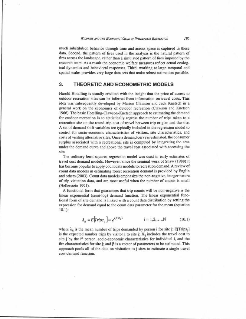
A functional fonn that guarantees that trip counts will be non-negative is the linear exponential (semi-log) demand function. The linear exponential func­tional fonn of site demand is linked with a count data distribution by setting the expression for demand equal to the count data parameter for the mean (equation 10.1):

i = 1,2, ..... N (10.1)

where A.ij is the mean number of trips demanded by person i for site j; E[Tripsjj] is the expected number trips by visitor i to site j; Xjj includes the travel cost to site j by the ith person, socio-economic characteristics for individual i, and the fire characteristics for site j; and ~ is a vector of parameters to be estimated. This approach pools all of the data on visitation to j sites to estimate a single travel cost demand function.

196 ENGUN, HOLMES, AND LU1Z

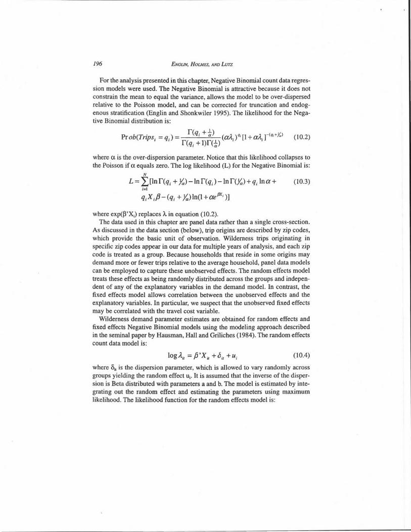
For the analysis presented in this chapter, Negative Binomial count data regres­sion models were used. The Negative Binomial is attractive because it does not constrain the mean to equal the variance, allows the model to be over-dispersed relative to the Poisson model, and can be corrected for truncation and endog­enous stratification (Englin and Shonkwiler 1995). The likelihood for the Nega­tive Binomial distribution is:

r(q . +1.) Prob(Trips . =q.)= I a (aA.)qj [1 +aA·r(q;+Ya) (10.2)

I I r(qj + l)r(-}) I I

where ex is the over-dispersion parameter. Notice that this likelihood collapses to the Poisson if ex equals zero. The log likelihood (L) for the Negative Binomial is:

N

L = L[lnr(qj + Ya)-lnr(qj)-lnr(Ya)+qj lna+ (10.3) ;=1

where exp(WXi ) replaces A. in equation (10.2). The data used in this chapter are panel data rather than a single cross-section.

As discussed in the data section (below), trip origins are described by zip codes, which provide the basic unit of observation. Wilderness trips originating in specific zip codes appear in our data for multiple years of analysis, and each zip code is treated as a group. Because households that reside in some origins may demand more or fewer trips relative to the average household, panel data models can be employed to capture these unobserved effects. The random effects model treats these effects as being randomly distributed across the groups and indepen­dent of any of the explanatory variables in the demand model. In contrast, the fixed effects model allows correlation between the unobserved effects and the explanatory variables. In particular, we suspect that the unobserved fixed effects may be correlated with the travel cost variable.

Wilderness demand parameter estimates are obtained for random effects and fixed effects Negative Binomial models using the modeling approach described in the seminal paper by Hausman, Hall and Griliches (1984). The random effects count data model is:

logA jt = P'Xit +(jit +u j (1004)

where Oil is the dispersion parameter, which is allowed to vary randomly across groups yielding the random effect ui • It is assumed that the inverse of the disper­sion is Beta distributed with parameters a and b. The model is estimated by inte­grating out the random effect and estimating the parameters using maximum likelihood. The likelihood function for the random effects model is:

WILDFIRE AND THE ECONOMIC VALUE OF WIWERNESS RECREATION

P [ ] (ll r( Ait + q it ) ) r q il , •.. , q iT = X

r(Ait )r(qit + 1)

r(a +b)r(a + LtAit)r(b+ Lr q;,)

r(a)r(b)r(a+b+ Lt Ait + Lt qit )

197

(10.5)

where rn is the gamma function. Because this model adds a heterogeneity term to a model that already contains a heterogeneity term (the over-dispersion param­eter), Greene (2002, p. E20-120) warns that the random effects Negative Bino­mial model might be over-parameterized and convergence might not be attained. However, as shown in the Results section below, random effects were success­fully estimated using this model on the permit data.

The fixed effects count data model is:

(10.6)

where (Xi is the fixed effect. For the fixed effects model, the joint probability of the counts for each group is conditioned on the sum of the counts for the group (which solves the incidental parameters problem), and is estimated using condi­tional maximum likelihood. The conditional likelihood of the fixed effects nega­tive binomial is:

P [ If = rCLtAit)rCLtqit +1)rr rCA;t +qit) r qil, .. ·,qiT L.tqi/] r(~ '1 ~) rc'l. )r( . +1)

1=1 £..1 /l,it + £..t q it t /I"t q It (10.7)

Notice that the conditional likelihood function eliminates the fixed effect and the probability is.a function of ~ alone.

Once the parameters of the count data models are estimated, it is straight forward to estimate consumer surplus by integrating the area under the demand curve. Because the estimator used to obtain parameter estimates is nonlinear, total consumer surplus is found by simulating the demand equation using observed values for the explanatory variables. For the linear exponential demand function, total consumer surplus is estimated as: .

pi ACP'X) Consumer surplus = f Adp = (-1). (10.8)

pO Ptc

where po is the actual travel cost, pi is the choke price, and J}tc is the parameter estimate on the travel cost variable. Marshallian consumer surplus per trip (-1/ ~tc) is computed by dividing the total consumer surplus by the number of trips (A).

198 ENGUN, HOLMES, AND Lun

Because wildfires are included as an additive term in the vector of explanatory variable (X) in the regression model, wildfires affect the number of trips taken to Wilderness areas, but not the value per trip.2 The change in consumer surplus induced by wildfires occurring during various periods antecedent to the time of a visit is estimated by computing A(WX) with and without fires of specific vintages:

1&,({3' X obs) - 2({3' X vintage) Wildfire ~ in Consumer surplus = -"'----------'----

{3,c (10.9)

where xobs is the vector of explanatory variables set at their observed level for the simulation, and xvintage substitutes counterfactual area burned for fires of specific vintages. Note that equation (10.9) allows us to estimate the total change in trips resulting from wildfires of different vintages and sizes, but it does not allow us to determine whether specific groups are changing their recreational behavior (such as new entrants).

4. DATA

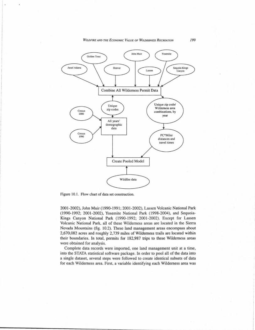
The analysis presented in this chapter required merging data assembled from three sources: (1) Wilderness permit data, (2) socio-economic data, and (3) wild­fire data (fig. 10.1). An explanation of these data and how they were merged is presented below.

4.1 Wilderness Permit Data

Visitors to National Forest and National Park Wilderness areas are required to obtain a permit before entry. For the purpose of recreation economic research, the key information provided by a Wilderness permit is the locatioh of the visi­tor's place of residence (zip code), which can be used to estimate travel distance from the place of residence to the Wilderness area.

In an attempt to collect as much permit data as possible from Wilderness areas throughout the mountainous regions of California, our permit data search process began with phone calls to National Forest ranger stations and National Park offices. Of the offices that maintained permit data for 1 or more years, appointments were made to meet with the data managers. Prior research had yielded permit data for several California Wilderness areas for the years 1990-1992. The current research effort yielded new permit data and the complete data set included the following Wilderness areas (and years): Ansel Adams (1990-1992; 2001-2002), Golden Trout (1990-1992; 2001-2002), Hoover (1990-1992;

2 As noted in the Conclusion section of this chapter, future research will be conducted to evaluate whether or not wildfires affect the value of a trip as well as the number of trips taken.

WILDFIRE AND THE ECONOMIC VALUE OF WILDERNESS RECREATION 199

Figure 10.1. Row chart of data set construction.

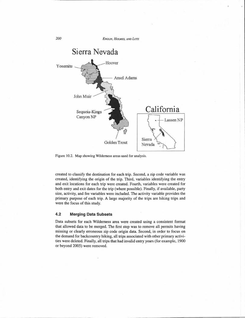
2001-2002), John Muir (1990-1991; 2001-2002), Lassen Volcanic National Park (1990-1992; 2001-2002), Yosemite National Park (1998-2004), and Sequoia­Kings Canyon National Park (1990-1992; 2001-2002). Except for Lassen Volcanic National Park, all of these Wilderness areas are located in the Sierra Nevada Mountains (fig. 10.2). These land management areas encompass about 2,670,082 acres and roughly 2,739 miles of Wilderness trails are located within their boundaries. In total, permits for 182,987 trips to these Wilderness areas were obtained for analysis.

Complete data records were imported, one land management unit at a time, into the STATA statistical software package. In order to pool all of the data into a single dataset, several steps were followed to create identical subsets of data for each Wilderness area. First, a variable identifying each Wilderness area was

200 ENGUN, HOLMES, AND LUTZ

Sierra Nevada

Yosemite

Sequoia -Kings CanyonNP

Hoover

Golden Trout

California Lassen NP

Figure 10.2. Map showing Wilderness areas used for analysis.

created to classify the destination for each trip. Second, a zip code variable was created, identifying the origin of the trip. Third, variables identifying the entry and exit locations for each trip were created. Fourth, variables were created for both entry and exit dates for the trip (where possible). Finally, if available, party size, activity, and fee variables were included. The activity variable provides the primary purpose of each trip. A large majority of the trips are hiking trips and were the focus of this study.

4.2 Merging Data Subsets

Data subsets for each Wilderness area were created using a consistent format that allowed data to be merged. The first step was to remove all permits having missing or clearly erroneous zip code origin data. Second, in order to focus on the demand for backcountry hiking, all trips associated with other primary activi­ties were deleted. Finally, all trips that had invalid entry years (for example, 1900 or beyond 2005) were removed.

WILDFIRE AND THE ECONOMIC VALUE OF W1WERNESS RECREATION 201

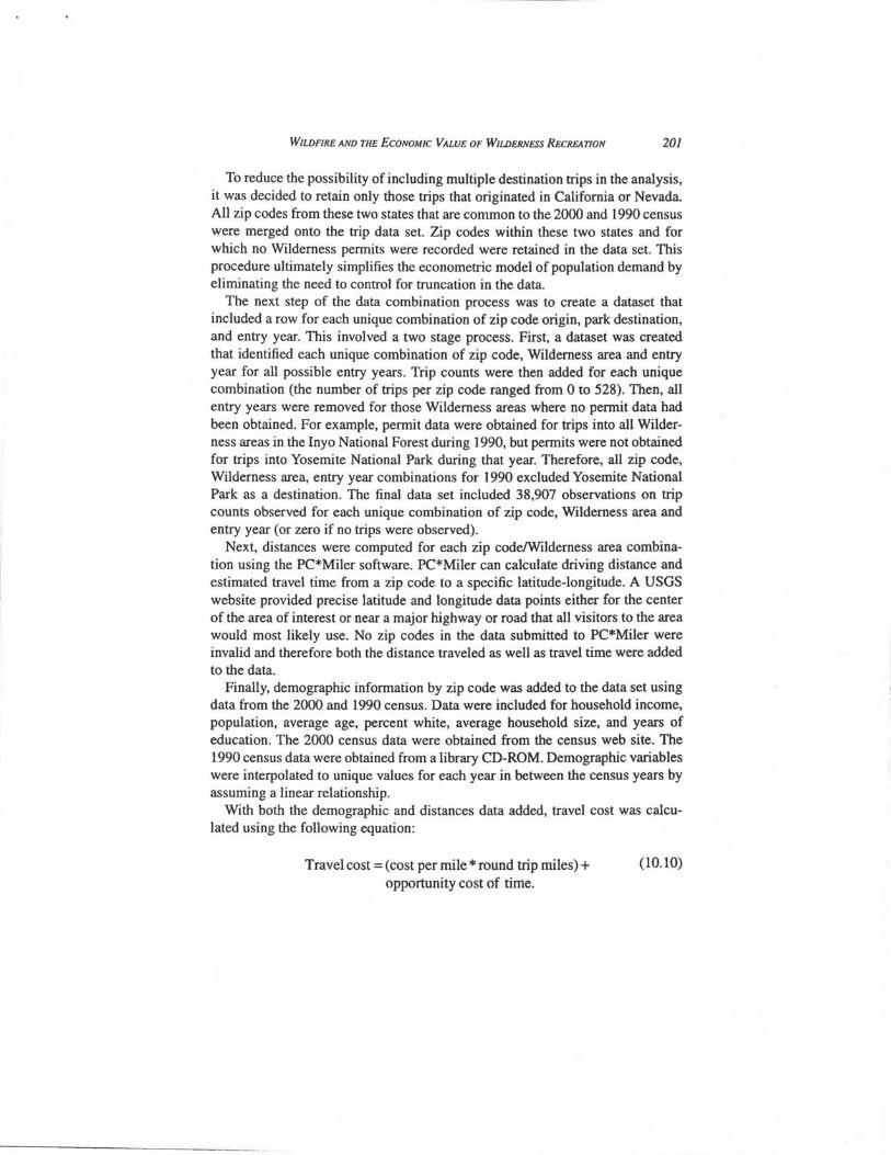
To reduce the possibility of including multiple destination trips in the analysis, it was decided to retain only those trips that originated in California or Nevada. All zip codes from these two states that are common to the 2000 and 1990 census were merged onto the trip data set. Zip codes within these two states and for which no Wilderness permits were recorded were retained in the data set. This procedure ultimately simplifies the econometric model of population demand by eliminating the need to control for truncation in the data.

The next step of the data combination process was to create a dataset that included a row for each unique combination of zip code origin, park destination, and entry year. This involved a two stage process. First, a dataset was created that identified each unique combination of zip code, Wilderness area and entry year for all possible entry years. Trip counts were then added for each unique combination (the number of trips per zip code ranged from 0 to 528). Then, all entry years were removed for those Wilderness areas where no pennit data had been obtained. For example, permit data were obtained for trips into all Wilder­ness areas in the Inyo National Forest during 1990, but permits were not obtained for trips into Yosemite National Park during that year. Therefore, all zip code, Wilderness area, entry year combinations for 1990 excluded Yosemite National Park as a destination. The final data set included 38,907 observations on trip counts observed for each unique combination of zip code, Wilderness area and entry year (or zero if no trips were observed).

Next, distances were computed for each zip codelWilderness area combina­tion using the PC*Miler software. PC*Miler can calculate driving distance and estimated travel time from a zip code to a specific latitude-longitude. A USGS website provided precise latitude and longitude data points either for the center of the area of interest or near a major highway or road that all visitors to the area would most likely use. No zip codes in the data submitted to PC*Miler were invalid and therefore both the distance traveled as well as travel time were added to the data.

Finally. demographic information by zip code was added to the data set using data from the 2000 and 1990 census. Data were included for household income, population, average age, percent white, average household size, and years of education. The 2000 census data were obtained from the census web site. The 1990 census data were obtained from a library CD-ROM. Demographic variables were interpolated to unique values for each year in between the census years by assuming a linear relationship.

With both the demographic and distances data added, travel cost was calcu­lated using the following equation:

Travel cost = (cost per mile * round trip miles) + opportunity cost of time.

(10.10)

202 ENGUN, HOLMES, AND LU1Z

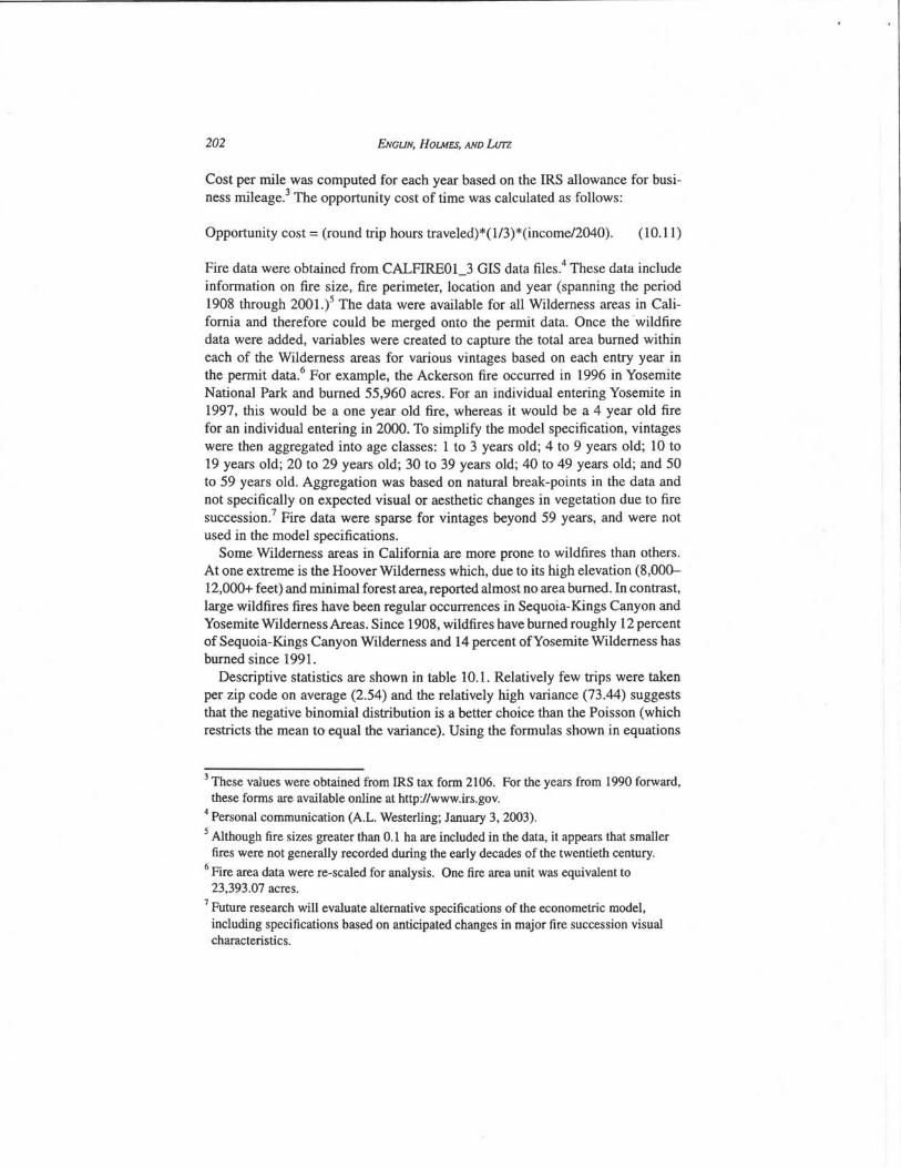
Cost per mile was computed for each year based on the IRS allowance for busi­ness mileage.3 The opportunity cost of time was calculated as follows:

Opportunity cost = (round trip hours traveled)*(1/3)*(income/2040). (10.11)

Fire data were obtained from CALFIREOl_3 GIS data files. 4 These data include infonnation on fire size, fire perimeter, location and year (spanning the period 1908 through 2001.i The data were available for all Wilderness areas in Cali­fornia and therefore could be merged onto the permit data. Once the 'wildfire data were added, variables were created to capture the total area burned within each of the Wilderness areas for various vintages based on each entry year in the permit data.6 For example, the Ackerson fire occurred in 1996 in Yosemite National Park and burned 55,960 acres. For an individual entering Yosemite in 1997, this would be a one year old fire, whereas it would be a 4 year old fire for an individual entering in 2000. To simplify the model specification, vintages were then aggregated into age classes: 1 to 3 years old; 4 to 9 years old; 10 to 19 years old; 20 to 29 years old; 30 to 39 years old; 40 to 49 years old; and 50 to 59 years old. Aggregation was based on natural break-points in the data and not specifically on expected visual or aesthetic changes in vegetation due to fire succession.7 Fire data were sparse for vintages beyond 59 years, and were not used in the model specifications.

Some Wilderness areas in California are more prone to wildfires than others. At one extreme is the Hoover Wilderness which, due to its high elevation (8,000-12,000+ feet) and minimal forest area, reported almost no area burned. In contrast, large wildfires fires have been regular occurrences in Sequoia-Kings Canyon and Yosemite Wilderness Areas. Since 1908, wildfires have burned roughly 12 percent of Sequoia-Kings Canyon Wilderness and 14 percent of Yosemite Wilderness has burned since 1991.

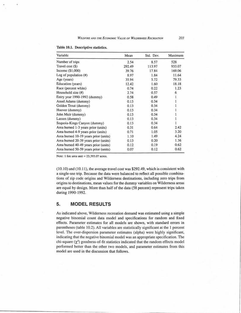
Descriptive statistics are shown in table 10.1. Relatively few trips were taken per zip code on average (2.54) and the relatively high variance (73.44) suggests that the negative binomial distribution is a better choice than the Poisson (which restricts the mean to equal the variance). Using the fonnulas shown in equations

3 These values were obtained from IRS tax form 2106. For the years from 1990 forward, these forms are available online at http://www.irs.gov.

4 Personal communication (A.L. Westerling; January 3, 2003).

5 Although fire sizes greater than 0.1 ha are included in the data, it appears that smaller fires were not generally recorded during the early decades of the twentieth century.

6 Fire area data were re-scaled for analysis. One fire area unit was equivalent to 23,393.07 acres.

7 Future research will evaluate alternative specifications of the econometric model, including specifications based on anticipated changes in major fire succession visual characteristics.

WILDFIRE AND THE ECONOMIC VALUE OF WILDERNESS RECREATION 203

Table! 10.1. Descriptive statistics.

Variable Mean Std. Dev. Maximum

Number of trips 2.54 8.57 528 Travel cost ($) 292.49 113.97 933.07 Income ($1,000) 39.76 17.84 169.06 Log of population (#) 8.97 l.84 1l.64 Age (years) 35.94 5.72 79.33 Education (years) 12.42 l.60 18.18 Race (percent white) 0.74 0.22 1.23 Household size (#) 2.74 0.57 6 Entry year 1990-1992 (dummy) 0.58 0.49 Ansel Adams (dummy) 0.13 0.34 Golden Trout (dummy) 0.13 0.34 Hoover (dummy) 0.13 0.34 John Muir (dummy) 0.13 0.34 Lassen (dummy) 0.l3 0.34 Sequoia-Kings Canyon (dummy) 0.l3 0.34 Area burned 1-3 years prior (units) 0.31 0.64 2.42 Area burned 4-9 years prior (units) 0.71 l.05 3.20 Area burned 10-19 years prior (units) 1.10 l.49 4.24 Area burned 20-39 years prior (units) 0.13 0.20 l.36 Area burned 40-49 years prior (units) 0.12 0.19 0.62 Area burned 50-59 years prior (units) 0.07 0.12 0.62

Note: 1 fire area unit = 23,393.07 acres.

(10.10) and (10.11), the average travel cost was $292.49, which is consistent with a single-use trip. Because the data were balanced to reflect all possible combina­tions of zip code origins and Wilderness destinations, including zero trips from origins to destinations, mean values for the dummy variables on Wilderness areas are equal by design. More than half of the data (58 percent) represent trips taken during 1990-1992.

5. MODEL RESULTS

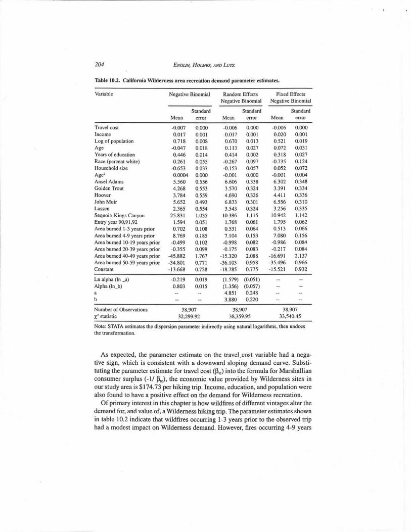
As indicated above, Wilderness recreation demand was estimated using a simple negative binomial count data model and specifications for random and fixed effects. Parameter estimates for all models are shown, with standard errors in parentheses (table 10.2). All variables are statistically significant at the 1 percent level. The over-dispersion parameter estimates (alpha) were highly significant, indicating that the negative binomial model was an appropriate specification. The chi-square (X2) goodness-of-fit statistics indicated that the random effects model performed better than the other two models, and parameter estimates from this model are used in the discussion that follows.

204 ENGUN, HOLMES. AND LUTZ

Table 10.2. California Wilderness area recreation demand parameter estimates.

Variable Negative Binomial Random Effects Fixed Effects Negative Binomial Negative Binomial

Standard Standard Standard Mean error Mean error Mean error

Travel cost -0.007 0.000 -0.006 0.000 -0.006 0.000 Income 0.017 0.001 0.017 0.001 0.020 0.001 Log of population 0.718 0.008 0.670 0.013 0.521 0.019 Age -0.047 0.018 0.113 0.027 0.072 0.031 Years of education 0.446 0.014 0.414 0.002 0.318 0.027 Race (percent white) 0.261 0.055 -0.267 0.097 -0.735 0.124 Household size -0.653 0.037 -0.153 0.057 0.052 0.072 Age2 0.0004 0.000 -0.001 0.000 -0.001 0.004 Ansel Adams 5.560 0.556 6.606 0.338 6.302 0.348 Golden Trout 4.268 0.553 3.570 0.324 3.391 0.334 Hoover 3.784 0.559 4.690 0.326 4.411 0.336 John Muir 5.652 0.493 6.833 0.301 6.556 0.310 Lassen 2.365 0.554 3.543 0.324 3.256 0.335 Sequoia-Kings Canyon 25.831 1.035 10.396 1.115 10.942 1.142 Entry year 90,91,92 1.594 0.051 1.768 0.061 1.795 0.062 Area burned 1-3 years prior 0.702 0.108 0.531 0.064 0.513 0.066 Area burned 4-9 years prior 8.769 0.185 7.104 0.153 7.080 0.156 Area burned 10-19 years prior -0.499 0.102 -0.998 0.082 -0.986 0.084 Area burned 20-39 years prior -0.355 0.099 -0.175 0.083 -0.217 0.084 Area burned 40-49 years prior -45.882 1.767 -15.320 2.088 -16.691 2.137 Area burned 50-59 years prior -34.801 0.771 -36.103 0.958 -35.496 0.966 Constant -13.668 0.728 -18.785 0.775 -15.521 0.932

Ln alpha (In _a) -0.219 0.019 (1.579) (0.051) Alpha (In_b) 0.803 0.015 (1.356) (0.057) a 4.851 0.248 b 3.880 0.220

Number of Observations 38,907 38,907 38,907 X2 statistic 32,299.92 38,359.95 33,540.45

Note: STATA estimates the dispersipn parameter indirectly using natural logarithms, then undoes the transformation.

As expected, the parameter estimate on the travel, cost variable had a nega­tive sign, which is consistent with a downward sloping demand curve. Substi­tuting the parameter estimate for travel cost (~tc) into the formula for Marshallian consumer surplus (-1/ Ptc), the economic value provided by Wilderness sites in our study area is $174.73 per hiking trip. Income, education, and population were also found to have a positive effect on the demand for Wilderness recreation.

Of primary interest in this chapter is how wildfires of different vintages alter the demand for, and value of, a Wilderness hiking trip. The parameter estimates shown in table 10.2 indicate that wildfires occurring 1-3 years prior to the observed trip had a modest impact on Wilderness demand. However, fires occurring 4-9 years

WILDFIRE AND THE ECONOMIC VALUE OF WILDERNESS RECREATION 205

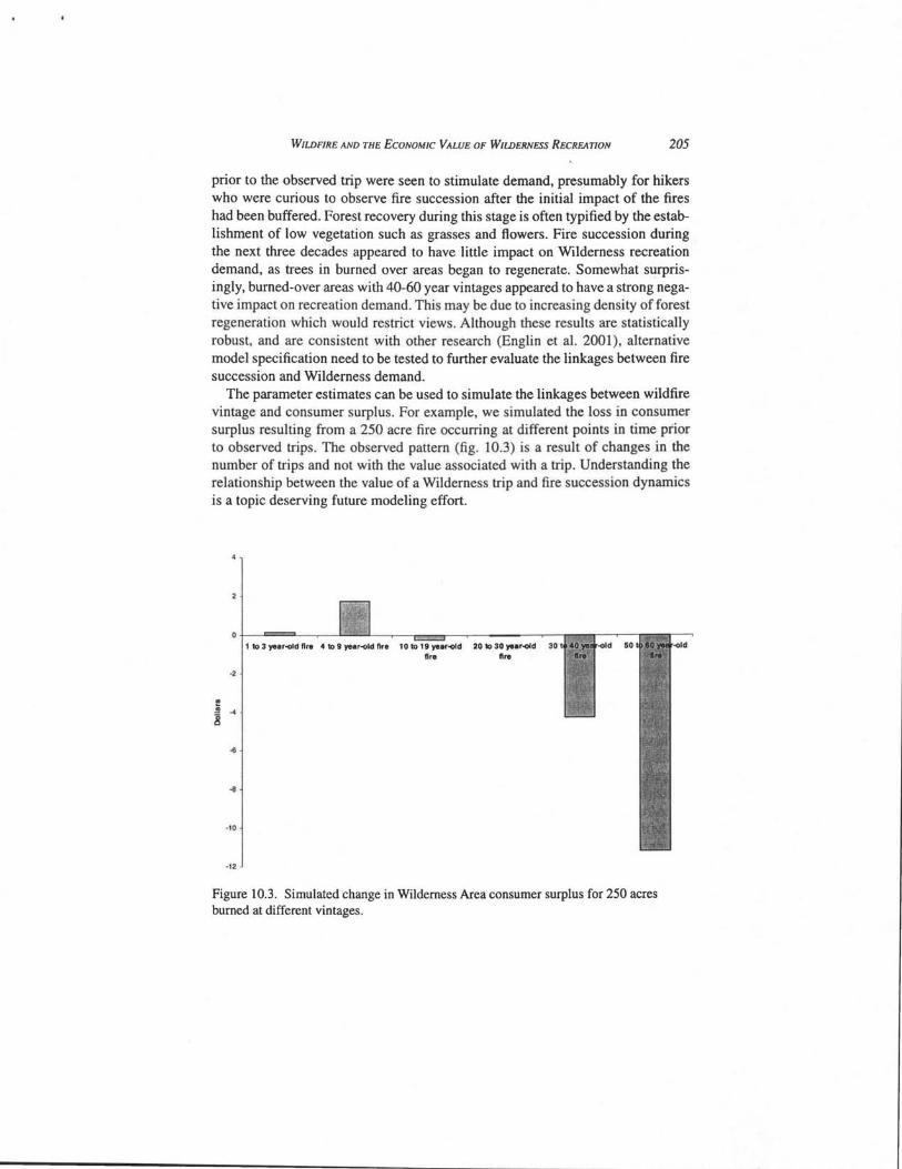
prior to the observed trip were seen to stimulate demand, presumably for hikers who were curious to observe fire succession after the initial impact of the fires had been buffered. Forest recovery during this stage is often typified by the estab­lishment of low vegetation such as grasses and flowers. Fire succession during the next three decades appeared to have little impact on Wilderness recreation demand, as trees in burned over areas began to regenerate. Somewhat surpris­ingly, burned-over areas with 40-60 year vintages appeared to have a strong nega­tive impact on recreation demand. This may be due to increasing density of forest regeneration which would restrict views. Although these results are statistically robust; and are consistent with other research (Englin et al. 2001), alternative model specification need to be tested to further evaluate the linkages between fire succession and Wilderness demand.

The parameter estimates can be used to simulate the linkages between wildfire vintage and consumer surplus. For example, we simulated the loss in consumer surplus resulting from a 250 acre fire occurring at different points in time prior to observed trips. The observed pattern (fig. 10.3) is a result of changes in the number of trips and not with the value associated with a trip. Understanding the relationship between the value of a Wilderness trip and fire succession dynamics is a topic deserving future modeling effort.

1 to 3 year-old fire 4 to 9 year-old fire 10 to 19 year-old 20 to 30 year-old 30 fire fire

-2

-10

·12

Figure 10.3. Simulated change in Wilderness Area consumer surplus for 250 acres burned at different vintages.

206 ENGUN, HOIMES, AND LuTZ

6. CONCLUSION

Although the analysis presented in this chapter is exploratory, and should not be viewed as definitive, it represents the first attempt to estimate the effects of forest fires on recreation demand that exclusively uses observations on actual behavior and does not rely on responses to contingent behavior questions. Rela­tive to other studies that have modeled the impact of wildfires on outdoor recre­ation, the dataset presented here is enonnous. The model estimates are based on nearly 183,000 observations of actual Wilderness trips taken under a variety of conditions. The panel data set spans a decade and a half of Wilderness recreation behavior and is linked to a wildfire data set that spans nearly 6 decades. As the data cover such a long period of time, as well as including several alternative Wilderness destinations, an exceptionally broad range of demand substitution patterns is captured.

Based on our exploratory analysis, the major conclusion of this chapter is that fire succession is linked to Wilderness recreation demand in a complex fashion. Wildfires of recent vintages appear to increase the number of trips to Wilderness areas, and wildfires of older vintages appear to decrease the number of trips. The robust statistical results we obtained strongly suggest that Wilderness managers need to be aware of a potential flux in recreation demand for several years following large wildfires. The outward shift in demand we observed is consis­tent with visitation shifts reported for the Yellowstone fires of 1988 (Franke), with the Shenandoah fire complex of 2000 (Morton et al. 2003), the Rat Creek­Hatchery Creek fire in Leavenworth, Washington (Hilger 1998), and various fires in the intennountain western United States (Englin et al. 2001). It appears that a significant number of hikers and other outdoor recreation enthusiasts desire to observe fire behavior and its impacts on forest succession. We suggest that these demand shifts provide a good opportunity for land managers to provide educa­tional and scientific infonnation about fire ecology to this segment of the popula­tion. Further, volunteers might be recruited from among this demand segment to collect infonnation on fire succession, such as the location and abundance of plant species of interest. This pattern also suggests the need for sufficient resources to reduce potentially hazardous situations created by wildfires such as snag trees close to trails and campsites. Over the longer run, these results suggest that large areas burned by wildfires may begin to experience reductions in demand. Understanding these long-run demand shifts is important for trail and infrastructure planning in the impacted areas.

The data reported in this chapter are very rich and present analytical complexi­ties on many levels. As such, we conclude this chapter by suggesting various avenues for future research. First, wildfire area was treated as a linear variable in the analysis. However, future research should consider the possibility of non­linear responses to wildfires, perhaps occurring at different spatial thresholds and degrees of fire intensity (such as crown fires vs. low-intensity ground fires). Second, a precise understanding of why visitors seem to prefer recent fires to fires

WILDFIRE AND THE ECONOMIC VALUE OF WILDERNESS RECREATION 207

of older vintages is lacking, and this demand behavior might be clarified through on-site surveys of Wilderness users. Third, partitioning the data and perfonning micro studies could be illuminating. For example, it would be useful to identify demand shifts among substitute Wilderness areas in response to large, recent fires such as the 55,957 acre Ackerson fire in the Yosemite Wilderness. Not only would such analyses permit validation testing of the hypotheses evaluated in this large-scale study, but such micro-analyses would likely provide greater detail about the patterns of cross-sectional and inter-temporal substitution by Wilder­ness travelers. Finally, it is plausible that, in addition to affecting the number of Wilderness trips, wildfires might affect the quality and value of trips taken. This hypothesis will be tested in future research and should help to further clarify the effects of wildfires on the economic value of outdoor recreation.

7. REFERENCES

Bowker, J.M., D. Murphy, H.K. Cordell, D.B.K. English, 1.e. Bergstrom, C.M. Starbuck, e.J. Betz, and G.T. Green. 2006. Wilderness and primitive area recreation participa­tion and consumption: An examination of demographic and spatial factors. Journal of Agricultural and Applied Economics 38(2):317-326.

Boxall, P.c., D.O. Watson, and J. Englin. 1996. Backcountry recreationists' valuation of forest and park management features in wilderness parks of the western Canadian shield. Canadian Journal of Forest Research 26(6):982-990.

Butry, D.T., D.E. Mercer, J.P. Prestemon, 1.M. Pye, and T.P. Holmes. 2001. What is the price of catastrophic wildfire? Journal of Forestry 99:9-17.

Champ, P.A., K.J. Boyle, and T.C. Brown (eds.). 2003. A primer on non-market valuation. Kluwer Academic Publishers, Dordrecht, The Netherlands.

Clawson, M., and J.L. Knetsch. 1966. Economics of outdoor recreation. Johns Hopkins University Press, Baltimore, MD.

Englin,1.. and 1.S. Shonkwiler. 1995. Estimating social welfare using count data models: An application to long-run recreation demand under conditions of endogenous stratifi­cation and truncation. The Review of Economics and Statistics 77(1): 104-112.

Englin, J.E., T.P. Holmes, and E.O. Sills. 2003. Estimating forest recreation demand using count data models. Kluwer Academic Publishers, Dordrecht, The Netherlands.

Englin, J., J. Loomis, and A. Gonzalez-Caban. 2001. The dynamic path of recreational values following a forest fire: A comparative analysis of states in the Intermountain West. Canadian Journal of Forest Research 31(10):1837-1844.

Franke, M.A. 2000. Yellowstone in the afterglow: Lessons from the fires. Mammoth Hot Springs, WY: Yellowstone Center for Resources, Yellowstone National Park. Available online at http://www.nps.gov/archive/yeIVpublications/pdfs/fire/afterglow.htm.

Geary, T.E, and G.L. Stokes. 1999. Forest Service wilderness management. In: Outdoor Recreation in American Life: A National Assessment of Demand and Supply Trends (H.K. Cordell, Principal Investigator). Sagamore Publishing, Champaign, IL. p. 388-391.

208 ENGUN, HOlMES, AND LuIZ

Greene, W.H. 2002. Limdep Version 8: Econometric modeling guide. Econometric Software, Plainview, NY.

Hausman, J., B.H. Hall, and Z. Griliches. 1984. Econometric models for count data with \ an application to the patents-R&D relationship. Econometrica 52(4):909-938.

Hellerstein, D.M. 1991. Using count data models in travel cost analysis with aggregate data. American Journal of Agricultural Economics 73:860-867.

Hesseln, H., J.B. Loomis, and A. Gonzalez-Caban. 2003. Wildfire effects on hiking and biking demand in New Mexico: A travel cost study. Journal of Environmental Management 69(4):359-368.

Hesseln, H., J.B. Loomis, and A. Gonzalez-Caban. 2004. The effects of fire on recreation demand in Montana. Western Journal of Applied Forestry 19(1):47-53.

Hilger, J. 1998. A bivariate compound poisson application: The welfare effects of forest fire on wilderness day-hikers. M.S. Thesis, University of Nevada, Reno.

Kent, B., K. Gebert, S. McCaffrey, W. Martin, D. Calkin, E. Schuster, I. Martin, H.W. Bender, G. Alward, Y. Kumagai, P. Cohn, M. Carroll, D. Williams, and C. Ekarius. 2003. Social and economic issues of the Hayman Fire. Gen. Tech. Rep. RMRS-GTR-114. USDA Forest Service, Fort Collins, CO.

Loomis, J., K. Bonetti, and C. Echohawk. 1999. Demand for and supply of wilderness. In: Outdoor Recreation in American Life: A National Assessment of Demand and Supply Trends (H.K. Cordell, Principal Investigator). Sagamore Publishing, Champaign, IL. p.351-375.

Loomis, J., A. Gonzalez-Caban, and J. Englin. 20ot. Testing for differential effects of forest fires on hiking and mountain biking demand and benefits. Journal of Agricultural and Resource Economics 26(2):508-522.

Morton, D.C., M.E. Roessing, A.E. Camp, and M.L. Tyrell. 2003. Assessing the environ­mental, social, and economic impacts of wildfire. Yale University, School of Forestry and Environmental Studies, New Haven, CT. GISF Research Paper 001. 54 p.

Shaw, D. 1988. On-site samples' regression: Problems of non-negative integers, trunca­tion and endogenous stratification. Journal of Econometrics 37:211-223.

Vaux, H.J., Jr., P.D. Gardner, and TJ. Mills. 1984. Methods for assessing the impact of fire on forest recreation. Gen. Tech. Rep. PSW-79. USDA Forest Service, Albany, CA.

j •