Embed Size (px)
DESCRIPTION
RAP
Citation preview
Risk-Adjusted Performance Measurement –
State of the Art
Bachelor Thesis
of the University of St. Gallen
School of Business Administration,
Economics, Law and Social Sciences (HSG)
to obtain the title of
Bachelor of Arts (B.A.) in Business Administration
Submitted by:
Alexandra Wiesinger
Student-ID: 07-610-679
Referee: Prof. Dr. Karl Frauendorfer
University of St. Gallen (HSG), St. Gallen, Switzerland
St. Gallen, May 2010
II
Abstract
More than 100 alternative risk-adjusted performance measures can be identified in
literature, most of them attempting to remedy against the shortcoming of the Sharpe
Ratio which relies on normally distributed returns. However, there is a fervent
discussion in literature whether the choice of risk-adjusted performance measure
actually matters or not.
This work firstly provides an overview of the current state of the art of risk-adjusted
performance measurement by discussing the most frequently used risk-adjusted
performance measures in scientific literature and secondly investigates the question
whether different alternative performance measures lead to different investment
decisions compared to each other and to the Sharpe Ratio.
The discussed risk-adjusted performance measures are applied to the return
distribution of a portfolio of bank products. The analysis shows that the majority of the
examined performance measures produce rankings of investment alternatives which are
highly correlated to each other and to the Sharpe Ratio. Yet, contradicting the findings of
some authors, it is shown that the choice of performance measure and of underlying
parameters does matter. There are some measures which produce significantly different
results, which for some of them is caused by the choice of parameters.
III
Table of Contents
List of Figures .................................................................................................................................................. IV
List of Tables ................................................................................................................................................... IV
1. Introduction .............................................................................................................................................. 1
2. Risk-Adjusted Performance Measurement ................................................................................... 3
2.1. The need for Risk-Adjusted Performance Measurement ............................................... 3
2.2. Evolution of Risk-Adjusted Performance Measures ......................................................... 4
2.3. Literature Review .......................................................................................................................... 7
3. State of the Art of Risk-Adjusted Performance Measures ....................................................... 9
3.1. Categorization of Performance Measures ............................................................................ 9
3.2. Performance Measures based on Volatility ...................................................................... 10
3.2.1. Sharpe Ratio ......................................................................................................................... 10
3.2.2. Adjusted Sharpe Ratio ...................................................................................................... 11
3.3. Performance Measures based on Value-at-Risk ............................................................. 13
3.3.1. Excess Return on Value-at-Risk .................................................................................... 13
3.3.2. Conditional Sharpe Ratio ................................................................................................. 15
3.3.3. Modified Sharpe Ratio ...................................................................................................... 16
3.4. Performance Measures based on Lower Partial Moments ......................................... 17
3.4.1. Omega ..................................................................................................................................... 17
3.4.2. Sortino Ratio ........................................................................................................................ 19
3.4.3. Kappa 3 ................................................................................................................................... 20
3.4.4. Gain-Loss Ratio and Upside-Potential Ratio ............................................................ 20
3.4.5. Farinelli-Tibiletti Ratio ..................................................................................................... 21
3.5. Performance Measures based on Drawdown .................................................................. 23
3.5.1. Calmar Ratio ......................................................................................................................... 23
3.5.2. Sterling Ratio ........................................................................................................................ 23
3.5.3. Burke Ratio ........................................................................................................................... 24
4. Application of Risk- Adjusted Performance Measures .......................................................... 25
4.1. Performance Analysis................................................................................................................ 25
4.2. Variation of Methods and Parameters ................................................................................ 35
5. Conclusion .............................................................................................................................................. 42
References ....................................................................................................................................................... 44
Appendix .......................................................................................................................................................... 49
IV
List of Figures
Figure 1: Comparison of return distributions with different values of skewness ................ 6
Figure 2: Density function of loss and Value-at-Risk ..................................................................... 14
List of Tables
Table 1: General analysis of the return distributions ..................................................................... 25
Table 2: Q-Q-Plot Scenario E: E0 ............................................................................................................ 27
Table 3: Q-Q-Plot Scenario E: E1 ............................................................................................................ 27
Table 4: Q-Q-Plot Scenario E: E2 ............................................................................................................ 27
Table 5: Q-Q-Plot Scenario F: F0 ............................................................................................................. 28
Table 6: Q-Q-Plot Scenario F: F1 ............................................................................................................. 28
Table 7: Q-Q-Plot Scenario F: F2 ............................................................................................................. 28
Table 8: Results of the performance analysis .................................................................................... 30
Table 9: Ranking of the investment strategies .................................................................................. 31
Table 10: Rank correlations for scenario E ........................................................................................ 33
Table 11: Rank correlations for scenario F ........................................................................................ 34
Table 12: Parametric vs. Empirical EVaR and CSR .......................................................................... 36
Table 13: EVar, Conditional SR and Modified SR for different confidence levels ................ 37
Table 14: Omega/GLR and the FTR for different interest rates ................................................. 39
Table 15: Omega/GLR, the Sortino Ratio, Kappa 3 and UPR for different interest rates . 49
Table 16 : The versions of the FTR for different interest rates .................................................. 50
Table 17: Sterling Ratio and Burke Ratio for different numbers of drawdowns ................. 51
Alexandra Wiesinger Risk-Adjusted Performance Measurement
1
1. Introduction
“Does the choice of risk-adjusted performance measure matter?” This is the question the
current discussion in academic literature revolves around. Risk-adjusted performance
measures are an important tool for investment decisions. Whenever an investor
evaluates the performance of an investment he will not only be interested in the
achieved absolute return but also in the risk-adjusted return – i. e. in the risk which had
to be taken to realize the profit.
The first ratio to measure risk-adjusted return was the Sharpe Ratio introduced by
William F. Sharpe in 1966. Although being frequently used in theory and practice the
Sharpe Ratio has a major drawback as it is designed for the use in a µ-σ- framework and
thus requires returns to be normally distributed. The events of the current financial
crisis have shown clearly that this assumption does not hold true and that especially
events at the tails of the distribution – most importantly high losses – are more likely
than assumed by the normal distribution. As a result, the Sharpe Ratio might lead to
inaccurate investment decisions.
In the past years a flood1 of alternative risk-adjusted performance measures which
mostly do not rely on normally distributed returns have been developed in literature in
order to remedy against this shortcoming of the Sharpe Ratio. The creators of the new
performance measures2 try to prove that their respective ratios are able to produce
more accurate results than the Sharpe Ratio. To verify this claim, some authors have
attempted – mostly using hedge fund returns – to explore the differences in
performance results between the Sharpe Ratio and the alternative performance
measures in order to determine the usefulness of the newer performance measures. But
so far the results have been ambiguous.
This work aims at adding on to the ongoing discussion about risk-adjusted performance
measures. The first objective is to provide an overview of the current state of the art of
risk-adjusted performance measurement by describing and discussing the most
frequently used risk-adjusted performance measures in scientific literature. Secondly,
1 In a comprehensive study Cogneau and Hübner (2009) identified more than 101 ways to measure
performance. 2 For reasons of better legibility risk-adjusted performance measure in this work simply shall be referred
to as performance measures.
Alexandra Wiesinger Risk-Adjusted Performance Measurement
2
following other authors, it shall be determined whether the described alternative
performance measures indeed lead to other investment decisions than the Sharpe Ratio
respectively if they yield different results in comparison to each other. This is done by
applying the performance measures to a portfolio of bank products, an asset class which
has not been used for this kind of analysis before.
This work is divided into four parts. The first part describes the fields of application of
risk-adjusted performance measurement and the theoretical need for alternative
performance measures is highlighted. Furthermore a literature review of studies which
compare the results of traditional performance measures to those of alternative
measures shall be provided. The second part is devoted to the description and critical
discussion of risk-adjusted performance measures. In the third part the performance
measures described in part two are applied to measure the performance of a portfolio of
bank products and variations in the assumed parameters are conducted to test the
resistance of the performance results. Finally, the findings of this work shall be
summarized in the fourth part.
Alexandra Wiesinger Risk-Adjusted Performance Measurement
3
2. Risk-Adjusted Performance Measurement
2.1. The need for Risk-Adjusted Performance Measurement
Risk-adjusted performance Measurement encompasses a set of concepts. Those
concepts may vary in detail depending on the context they are used in. However, all risk-
adjusted performance measures have one thing in common: they compare the return on
capital to the risk taken to earn this return – i.e. some kind of risk-adjustment is
adopted. Generally speaking, return in risk-adjusted performance measures is measured
either by absolute returns or by relative returns (i.e. excess returns), whereas
disagreement prevails in literature on how exactly risk should be taken into account.
This has given rise to the development of a considerable number of alternative risk-
adjusted performance measures. Thus, risk-adjusted performance measures can take
many forms as shall be shown in the following chapters.
In the past years risk-adjusted performance measures have gained great importance.
The first reason for this development is the emergence of investment funds as an
important investment category. Investors needed an effective tool to evaluate the
respective performance of the various funds compared to the risk taken by the fund
managers to choose the right option for capital allocation (Weisman, 2002, p. 80). The
second reason is the introduction of the Basel II regulatory framework, which requires
financial institutions to hold a certain amount of equity as a cushion against unexpected
losses for each risky position taken. As a result financial institutions have a great
interest in efficiently allocating capital not only according to the resulting return but also
to the risk shouldered and
Therefore, banks more and more turn to concepts based on risk-adjusted performance
measures like Risk-adjusted Return on Capital (RAROC) when evaluating their business
activities (Smithson, Brannan, Mengle & Zmiewski., 2003, p. 5). Due to these
developments, risk-adjusted performance measures gradually replace traditional
performance measures like Return on Equity (ROE) or Return on Investment (ROI)
when it comes to analyzing performance in financial contexts as these traditional
measures do not take into account risk (Zimmermann & Wegmann, 2003, p. 33).
As indicated above, risk-adjusted performance measurement has two major fields of
application- performance evaluation and capital allocation. In the field of performance
Alexandra Wiesinger Risk-Adjusted Performance Measurement
4
evaluation, risk-adjusted performance measures are used to rank competing investment
strategies ex-ante and ex-post according to their respective risk-adjusted returns. The
investment with the highest return and the lowest risk ranks first (Jorion, 2006, p. 291).
A further application in this context is the design of compensation plans for traders or
asset managers. If their performance is assessed according to the raw profits they make,
they will seek to take risk to maximize their bonuses. In contrast, in a risk-adjusted
compensation framework, excessive risk-taking can be avoided as employees are
compensated according to their risk-adjusted profits. (Dowd, 2002, p. 210)
Risk-adjusted performance measurement is also used to guide management in efficient
internal capital allocation. It helps the management of financial institutions to evaluate
the risk-adjusted performance of their business units, traders or investment portfolios.
Like this capital is only allocated to deals which are profitable from a risk-adjusted
performance point of view as equity is rare and expensive due to the minimum capital
requirements stated in the Basel II framework (McNeil, Embrechts & Frey,. 2005, p. 44).
The focus of this composition is on the use of risk-adjusted performance measurement
in the field of performance evaluation of investment opportunities. For an overview of
the application of risk-adjusted performance measurement for risk capital allocation in
banks and risk-adjusted management of entire financial institutions see for example
Lister (1997).
2.2. Evolution of Risk-Adjusted Performance Measures
The Sharpe Ratio, introduced by William F. Sharpe in his seminal Journal of Business
article in 1966, can be regarded as the first risk-adjusted performance measure. Due to
its simplicity and thus easy application it has found widespread acceptance in literature
and in practice. The Sharpe Ratio measures risk by volatility, which reflects the
paradigm of the Modern Portfolio Theory prevalent during the genesis of the Sharpe
Ratio.
The concept of volatility represents one of the major shortcomings of the Sharpe Ratio.
Firstly, volatility does not treat variability in gains and variability in losses separately–
i.e. the Sharpe Ratio penalizes for both downside and upside variability in returns. A
rational investor, however, distinguishes between gains and losses and would rather
consider high variability in gains to be an attractive reward potential (Zakamouline,
Alexandra Wiesinger Risk-Adjusted Performance Measurement
5
2010, p. 14). Yet, measuring risk-adjusted performance with the Sharpe Ratio might lead
to the fact that an asset with a high upside volatility is ranked lower than an asset with a
low downside volatility.
Secondly, if volatility is used to measure risk, normally distributed returns are assumed.
However, starting with the research of Mandelbrot (1963), many empirical studies have
proven that the theoretical assumption of normally distributed returns does not hold
true for many asset classes. There is a considerable body of literature (e.g. Ekholm &
Pasternack, 2005; Leland, 2002; Aparicio & Estrada, 2001) which demonstrates that
returns are not normally distributed but often show ‘fat tails’ – i.e. that extreme events
are more likely than predicted by the normal distribution. This has practically been
proven by several financial crises in the past. For alternative investment forms like
hedge funds researchers (e.g. Brooks & Kat, 2002; Malkiel & Saha, 2005; Kosowski, Naik
& Teo, 2007) have shown that this asset class especially exhibits significant amounts of
skewness with rare but extreme gains or losses due to their dynamic trading strategies
and their holding of derivatives. That is why some authors (e.g. Hodges, 1998; Bernardo
& Ledoit, 2000) conclude that performance evaluation with the Sharpe Ratio seems
dubious if returns are non-normally distributed, which shall be illustrated by the
following example from Guse and Rudolf (2008, p. 198).
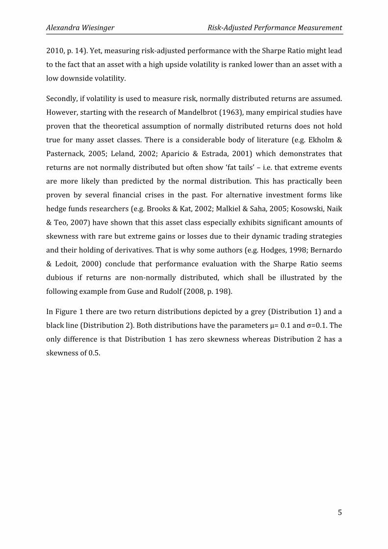
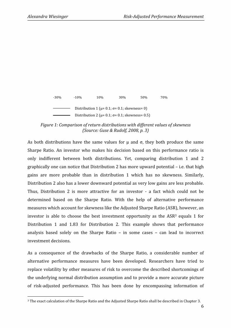
In Figure 1 there are two return distributions depicted by a grey (Distribution 1) and a
black line (Distribution 2). Both distributions have the parameters µ= 0.1 and σ=0.1. The
only difference is that Distribution 1 has zero skewness whereas Distribution 2 has a
skewness of 0.5.
Alexandra Wiesinger
-30% -10%
Distribution 1
Distribution 2
Figure 1: Comparison of return dist(Source: Guse & Rudolf, 200
As both distributions have the same
Sharpe Ratio. An investor who makes his decision
only indifferent between both distributions. Yet, comparing distribution 1 and 2
graphically one can notice that D
gains are more probable than in distribution 1 which has no skewness. Similarly,
Distribution 2 also has a lower downward potential as very low gains are less probable.
Thus, Distribution 2 is more attractive f
determined based on the Sharpe Ratio. With the help of alternative performance
measures which account for skewness
investor is able to choose the best investment o
Distribution 1 and 1.83 for
analysis based solely on the Sharpe Ratio
investment decisions.
As a consequence of the drawbacks of
alternative performance measures
replace volatility by other measures of risk
the underlying normal distribution assumption
of risk-adjusted performance. This has been done by
3 The exact calculation of the Sharpe Ratio and the Adjusted Sharpe Ratio shall be described in Chapter 3.
Risk-Adjusted Performance Measurement
10% 30% 50% 70%
Distribution 1 (µ= 0.1; σ= 0.1; skewness= 0)
Distribution 2 (µ= 0.1; σ= 0.1; skewness= 0.5)
: Comparison of return distributions with different values of (Source: Guse & Rudolf, 2008, p. 3)
As both distributions have the same values for µ and σ, they both produce the same
Sharpe Ratio. An investor who makes his decision based on this performance ratio is
indifferent between both distributions. Yet, comparing distribution 1 and 2
raphically one can notice that Distribution 2 has more upward potential
gains are more probable than in distribution 1 which has no skewness. Similarly,
istribution 2 also has a lower downward potential as very low gains are less probable.
istribution 2 is more attractive for an investor - a fact which could not be
determined based on the Sharpe Ratio. With the help of alternative performance
measures which account for skewness like the Adjusted Sharpe Ratio (ASR)
the best investment opportunity as the ASR
Distribution 1 and 1.83 for Distribution 2. This example shows that performance
analysis based solely on the Sharpe Ratio – in some cases – can
of the drawbacks of the Sharpe Ratio, a considerable number of
alternative performance measures have been developed. Researchers have tried to
replace volatility by other measures of risk to overcome the described shortcomings of
normal distribution assumption and to provide a more
adjusted performance. This has been done by encompassing
The exact calculation of the Sharpe Ratio and the Adjusted Sharpe Ratio shall be described in Chapter 3.
Adjusted Performance Measurement
6
70%
values of skewness
values for µ and σ, they both produce the same
based on this performance ratio is
indifferent between both distributions. Yet, comparing distribution 1 and 2
2 has more upward potential – i.e. that high
gains are more probable than in distribution 1 which has no skewness. Similarly,
istribution 2 also has a lower downward potential as very low gains are less probable.
a fact which could not be
determined based on the Sharpe Ratio. With the help of alternative performance
like the Adjusted Sharpe Ratio (ASR), however, an
as the ASR3 equals 1 for
shows that performance
lead to incorrect
a considerable number of
esearchers have tried to
to overcome the described shortcomings of
and to provide a more accurate picture
ing information of
The exact calculation of the Sharpe Ratio and the Adjusted Sharpe Ratio shall be described in Chapter 3.

Alexandra Wiesinger Risk-Adjusted Performance Measurement
7
higher moments of distributions like skewness and kurtosis as well as by developing
measures which do not assume any distribution at all and therefore are generally
applicable – regardless of the return distribution.
2.3. Literature Review
As indicated in the introduction, there is a growing body of literature which tries to
determine whether the information contained in higher moments of distributions is
significant for performance results and thus, whether alternative performance measures
indeed lead to different rankings compared to the Sharpe Ratio and compared to each
other. In this section an overview of the most important contributions to this topic shall
be given.
Pedersen and Rudholm-Alfvin (2003) examine the performance of financial institution
stocks using a choice of traditional and alternative performance measures partly
identical to the selection used in this work. They find that the rankings of the alternative
performance measures are extremely positively correlated among each other and to the
Sharpe Ratio. As the alternative performance measures do not lead to significantly
different results compared to the Sharpe Ratio in their analysis, the authors recommend
staying with this traditional measure as it is analytically convenient and traditionally
supported by researchers and practitioners (Pedersen & Rudholm-Alfvin, p. 166).
Motivated by these findings, Eling and Schumacher (2006) analyze the performance of
different categories of hedge funds using the Sharpe Ratio and a selection of the most
documented alternative performance measures similar to those described in this work.
Their results show high correlations in the rankings across all performance measures as
well. They further prove that the rankings are very robust to changes in underlying
parameters. Thus, they conclude that the choice of the performance measure does not
matter and that the Sharpe Ratio is sufficient for appraising risk-adjusted performance.
Using another sample of hedge fund returns, Glawischnig (2007) attempts to refute
Eling and Schumacher (2006) by showing that the choice of performance measure has a
considerable influence on the ranking. His analysis, however, also yields highly
correlated rankings for all performance measures. Nevertheless, this author warns
against dismissing the alternative performance measures. He points out that it is
necessary to include the information contained in the higher moments of distributions
Alexandra Wiesinger Risk-Adjusted Performance Measurement
8
even if they lead to the same result for the majority of observations. Yet, for some
investment alternatives the additional information might lead to alterations in the
ranking, which, even if small, might be significant for the decision of a particular investor
(Glawischnig, 2007, p. 27).
Heidorn (2009) also intends to disprove Eling and Schumacher (2006) based on hedge
fund returns. He partly succeeds as he is able to demonstrate that the rank order is
significantly heterogeneous with some of the middle-ranking indices whereas the
indices ranking best respectively worst are mostly the same. Furthermore he shows that
some alternative performance measures, mainly those based on drawdown, lead to
different rankings when a different method for evaluating ranking correlations is used.
From an overall point of view, however, his findings are the same as those from Eling
and Schumacher (2006), with highly correlated rankings for the alternative performance
measures.
Zakamouline (2010) criticizes the database used by Eling and Schumacher (2006). He
argues that their conclusion is based on a short sampling period and a small subset of
performance measures and thus, is only of limited validity. Furthermore he critically
notes that the majority of hedge fund returns examined by Eling and Schumacher (2006)
were close to being normally distributed which might be an explanation for the high
correlation in ranks. Zakamouline (2010) shows in his own analysis that, despite high
rank correlations, the rankings produced by alternative performance measures are far
from being identical to the ranking produced by the Sharpe Ratio. He points out that
there are some performance measures – notably the Farinelli-Tibiletti Ratio – which
yield rather low rank correlations to the Sharpe Ratio.
Summarizing the studies cited above, the findings show that alternative performance
measures in general do not yield significantly different ranking results than the Sharpe
Ratio. However, there seem to be some performance measures which – under certain
circumstances – lead to significant differences in rankings and therefore, legitimate the
existence of this group of performance measures.
Except for the studies of Pedersen and Rudholm-Alfvin (2003) the discussed studies
were based on hedge fund returns. This asset class is often criticized for suffering from
severe selection biases (for a detailed discussion see for example Kaiser, Heidorn &
Alexandra Wiesinger Risk-Adjusted Performance Measurement
9
Roder, 2009, p. 9) which might put the hitherto obtained statements about the
usefulness of alternative performance measures into question. Hence, returns of the
asset class of bank products shall be used in this work to determine whether alternative
performance measures yield different results compared to the Sharpe Ratio.
3. State of the Art of Risk-Adjusted Performance Measures
3.1. Categorization of Performance Measures
The performance measures discussed in this composition can be categorized according
to the risk-measure applied in the respective measures. The particular groups are
performance measures based on either (simple) volatility, Value-at-Risk, Lower Partial
Moments or drawdown. Technically the performance measures based on Value-at-Risk
also use volatility to measure risk but they additionally consider other factors, like the
mean. Thus, for the performance measures using volatility two separate groups were
formed, a common way of categorization in scientific literature.
Furthermore, one can distinguish between performance measures which assume
normally distributed returns, measures which explicitly account for higher moments of
distribution and measures which implicitly account for higher moments of distribution
by not assuming any distribution at all. The first group consists of the Sharpe Ratio,
Excess Return on Value-at-Risk and the Conditional Sharpe Ratio if the underlying
Value-at-Risk and Conditional Value-at-Risk are computed with the parametric method.
The second group is formed by the Adjusted Sharpe Ratio and the Modified Sharpe
Ratio. The third group includes all performance measures based on Lower Partial
Moments or drawdown.
As mentioned in Chapter 1, the first aim of this composition is to give an overview of the
most frequently discussed and applied alternative performance measures in current
literature of risk-adjusted performance measurement. Thus, the discussion of the
performance measures in this piece of work does not claim to be a complete
enumeration of the entire body of measures in literature. Instead, the performance
measures have been selected by their prevalence in current literature.
Alexandra Wiesinger Risk-Adjusted Performance Measurement
10
3.2. Performance Measures based on Volatility
3.2.1. Sharpe Ratio
The first and most frequently used performance measure, which uses volatility as a risk
measure is the Sharpe Ratio (Sharpe, 1966) The Sharpe Ratio (SR), also often referred to
as “Reward to Variability”, divides the excess return of an asset i over a risk-free interest
rate by the asset’s volatility.
(1) SRi = ����
rid ....... mean asset return4
rf ......... risk-free interest rate
σi ......... standard deviation
As risk-averse investors prefer high returns and low volatility, the alternative with the
highest Sharpe Ratio should be chosen when assessing investment possibilities (Scott &
Horvath, 1980, p. 915).
Due to its simplicity and its easy interpretability the Sharpe Ratio has become one of the
most widely used risk-adjusted performance measures (Weisman, 2002, p. 81). Yet, as
indicated in the previous Chapter, there are some shortcomings of the Sharpe Ratio that
need to be considered when employing it. Firstly, the Sharpe Ratio assumes normally
distributed returns as it measures risk by volatility. Consequently, as shown in the
example, the Sharpe Ratio might lead to wrong investment decisions when returns
deviate from the normal distribution and in this case is not the right tool to measure
risk-adjusted performance (Ingersoll, Spiegel & Goetzmann, 2007). Secondly, studies
(Ingersoll et al., 2007, Leland, 1999) have shown that the Sharpe Ratio is prone to be
manipulated through so-called information-free trading strategies. With these strategies
a fund manager increases the fund’s performance by manipulative actions without
actually adding value (Ingersoll et al., 2007, p. 1540). This is especially appealing for
managers whose bonuses are correlated to the Sharpe Ratio of the assets they manage.
In order to increase the Sharpe Ratio, they realize a gain in an early stage of the
evaluation period and then invest the entire funds in a risk-free asset for the rest of the
4 This notation for the mean asset return and the risk-free interest rate - ri
d respectively rf shall henceforth
be used in this work for all measures which require these parameters.
Alexandra Wiesinger Risk-Adjusted Performance Measurement
11
period. As the risk-free asset has a volatility of zero, the Sharpe Ratio converges towards
infinity and so does the bonus of the manager (Ingersoll et al., 2007, p. 1541).
3.2.2. Adjusted Sharpe Ratio
As skewness and kurtosis of a return distribution, which both might influence an
investor’s decision, are the essential part of the Adjusted Sharpe Ratio and of other
performance measures discussed in this composition, a brief description of these
moments of distributions shall be given before the Adjusted Sharpe Ratio is introduced:
Skewness (S), the third standardized moment of a random variable, measures the
asymmetry of the probability distribution of a random variable (r) around the mean (µ).
It is defined by the formula below (Poddig, Dichtl & Petersmeier, 2003, p. 141).
(2) S = �� ∑ �����������
�
Skewness yields positive values for so-called right-skewed distributions in which the
major part of values is concentrated on the left side of the distribution. Negative values
for skewness indicate a left-skewed distribution with more values on the right side.
Applied to an investment context, skewness can be interpreted as a risk parameter.
Returns with a positively skewed distribution density exhibit a lower probability of
losses (with the same expected return) and a higher probability for positive extreme
values. Conversely, with negatively skewed distribution densities negative extreme
values are more likely. Thus, a risk-averse investor prefers returns with positively
skewed distributions (Poddig, Dichtl & Petersmeier, 2003, p. 142).
Kurtosis is the fourth standardized moment of a random variable and describes the
amount of “peakedness” of a distribution compared to the normal distribution. A
distribution with a high amount of “peakedness” shows a concentration of values around
the mean and at the tails of a distribution. Thus, the probability of extreme values is
higher than in the normal distribution. Consequently, risk-averse investors prefer return
distributions with low kurtosis. Kurtosis (E) is calculated by the formula below (Poddig,
Dichtl & Petersmeier, 2003, p. 143).
(3) E = �� ∑ �����������
� �3
Alexandra Wiesinger Risk-Adjusted Performance Measurement
12
The expression more precisely describes the amount of excess kurtosis over the normal
distribution as it already takes into account that the normal distribution has a kurtosis
of 3. Summing up the findings above, risk-averse investors prefer positively skewed
return distributions with low kurtosis.5 This fact is either explicitly or implicitly
accounted for in the risk-adjusted performance measures presented in the following
chapters.
The Adjusted Sharpe Ratio (ASR) belongs to the group of measures in which skewness
and kurtosis are explicitly included. Its creators Pezier and White (2006) were
motivated by the drawbacks of the Sharpe Ratio, especially those caused by the
assumption of normally distributed returns, and therefore suggested an Adjusted Sharpe
Ratio to overcome this deficiency.
The measure is derived from a Taylor series expansion of expected utility with an
exponential utility function. Keeping the first four terms of the expansion leads to the
formula of the ASR stated below, where SR stands for the original Sharpe Ratio, S for
skewness and E for excess kurtosis (Pezier & White, 2006, p. 15).
(4) ASRi = ��� �1 !"#$ ��� � ! %
&'$ ���&(
The ASR accounts for the fact that investors prefer positive skewness and negative
excess kurtosis, as it contains a penalty factor for negative skewness and positive excess
kurtosis. If S is negative and E is positive the ASR gets smaller compared to the
traditional Sharpe Ratio. If the returns are normally distributed S and E are equal to zero
and the formula for the Adjusted Sharpe Ratio yields the same values as the traditional
Sharpe Ratio.
5 For a detailed proof of an investor’s preference towards the moments of a distribution see Scott &
Horvath (1980).
Alexandra Wiesinger Risk-Adjusted Performance Measurement
13
3.3. Performance Measures based on Value-at-Risk
3.3.1. Excess Return on Value-at-Risk
The following group of risk-adjusted performance measures uses Value-at-Risk (VaR)
and its modification the Conditional Value-at-Risk (CVaR) to account for risk.
The popular concept of VaR describes the expected maximum loss over a target horizon
within a given confidence level α.6 For example, a 10-day VaR of 10 % at a α=0.05
confidence level means that the maximum loss in the next 10 days will not exceed 10%
of an asset’s value in 95% (=100(1-α)%) of all cases. Using these numbers for a total
asset value of 10 million, the VaR is 1 Mio. So in 95% of all cases the loss will not exceed
1 million in the next 10 days.
VaR has become an essential tool for communicating risk to managers, directors and
shareholders as it captures downside risk in a single figure which is easy to interpret. It
is derived from probability distributions and it can, for instance, be modeled by
considering the empirical distribution – i.e. by taking the [(1- α)* N]th realization of a
sample of n realizations as a measure for VaR. For a sample of 100 return observations
sorted in descending order, for example, the empirical VaR is the 95th return
observation. Other methods are simulation and parametric approximation - e.g. through
the parameters of the normal distribution (Eisele, 2004, p. 113). In this work the
parametric approximation shall be used first and then be compared to the results of the
empirical VaR.
Assuming normally distributed returns, the VaR of a long-position is calculated as a
quantile of the standard normal distribution at a certain confidence level α, using the
expected value – i.e. the mean - and the standard deviation (Jorion, 2006, p. 110).
�5� VaRi = – �rid zα*σi� α ….. confidence level
zα ..... quantile of the standard normal distribution
6 For a comprehensive discussion of the concept of Value-at-Risk and its applications see for example
Jorion (2006).
Alexandra Wiesinger
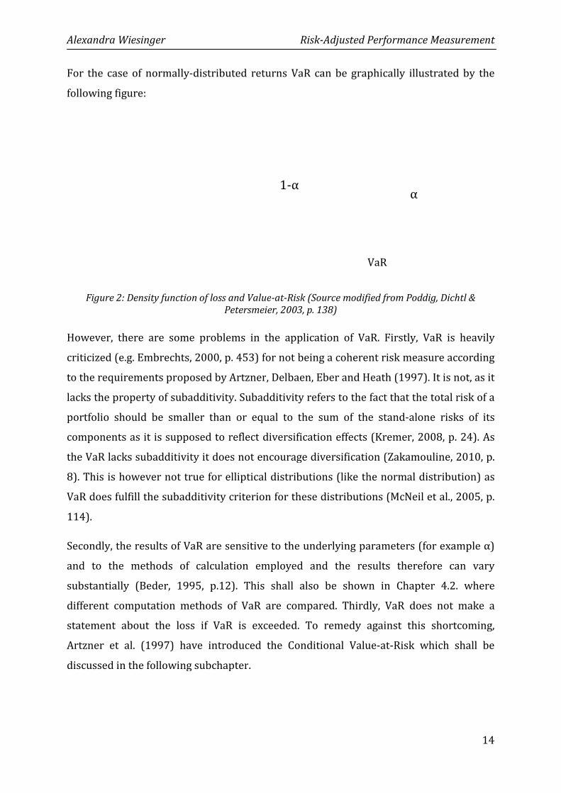
For the case of normally-distributed returns
following figure:
Figure 2: Density function of loss and Value
However, there are some problems in the application of VaR. Firstly
criticized (e.g. Embrechts, 2000
to the requirements proposed by Artzner
lacks the property of subadditivity. Subadditivity refers to the fact that the total risk of a
portfolio should be smaller
components as it is supposed to reflect
the VaR lacks subadditivity it does not encourage diversification (Zakamouline, 2010, p.
8). This is however not true
VaR does fulfill the subadditivity criterion
114).
Secondly, the results of VaR are sensitive to the underlying parameters
and to the methods of calculation employed and the
substantially (Beder, 1995, p.12
different computation methods of VaR are compared
statement about the loss if
Artzner et al. (1997) have introduced
discussed in the following subchapter
Risk-Adjusted Performance Measurement
distributed returns VaR can be graphically
function of loss and Value-at-Risk (Source modified from Poddig, Dichtl &Petersmeier, 2003, p. 138)
problems in the application of VaR. Firstly
Embrechts, 2000, p. 453) for not being a coherent risk measure according
to the requirements proposed by Artzner, Delbaen, Eber and Heath (1997)
lacks the property of subadditivity. Subadditivity refers to the fact that the total risk of a
portfolio should be smaller than or equal to the sum of the stand-
as it is supposed to reflect diversification effects (Kremer, 2008
the VaR lacks subadditivity it does not encourage diversification (Zakamouline, 2010, p.
This is however not true for elliptical distributions (like the normal distribution
the subadditivity criterion for these distributions (McNeil et al.
Secondly, the results of VaR are sensitive to the underlying parameters
ds of calculation employed and the results therefore
substantially (Beder, 1995, p.12). This shall also be shown in Chapter
different computation methods of VaR are compared. Thirdly, VaR does not make a
if VaR is exceeded. To remedy against this shortcoming
have introduced the Conditional Value-at-Risk which shall be
discussed in the following subchapter.
1-α
VaR
Adjusted Performance Measurement
14
graphically illustrated by the
modified from Poddig, Dichtl &
problems in the application of VaR. Firstly, VaR is heavily
a coherent risk measure according
(1997). It is not, as it
lacks the property of subadditivity. Subadditivity refers to the fact that the total risk of a
-alone risks of its
(Kremer, 2008, p. 24). As
the VaR lacks subadditivity it does not encourage diversification (Zakamouline, 2010, p.
like the normal distribution) as
(McNeil et al., 2005, p.
Secondly, the results of VaR are sensitive to the underlying parameters (for example α)
therefore can vary
Chapter 4.2. where
, VaR does not make a
To remedy against this shortcoming,
Risk which shall be
α
Alexandra Wiesinger Risk-Adjusted Performance Measurement
15
When VaR is used to assess risk-adjusted performance, the measure Excess Return on
VaR (EVaR) emerges. It was developed by Dowd (2002) and compares the excess return
of an asset to the VaR of the asset. EVaR can be calculated by the following formula.
�6� EVaRi = ����456
3.3.2. Conditional Sharpe Ratio
As mentioned above, in order to overcome the shortcoming of VaR, which does not
consider losses outside of the (1-α)-confidence interval, the Conditional Value-at-Risk
(CVaR) has been developed. CVaR describes the expected loss under the condition that
VaR is exceeded. Therefore only the values of the distribution that exceed the VaR are
considered when calculating CVaR. Following the interpretation of VaR as maximum
expected loss in 100*(1- α)% of cases, CVaR can be interpreted as average loss in
100*α% of cases (Albrecht & Koryciorz, 2003, p. 2). Similar to the VaR, CVaR can be
calculated either empirically or parametrically, using the parameters of the normal
distribution. In the case of normally distributed returns CVaR is described by the
following expression (Albrecht & Koryciorz, 2003, S. 6).
�7� CVaRi = 9�: ;�<�=>�? @�
N 1-α ... (1- α)- quantile of the standard normal distribution
A ......... density function of the standard normal distribution
It is shown by Acerbi & Tasche (2002) that CVaR is a coherent measure of risk as it
fulfills all axioms proposed by Artzner et al. (1997). Therefore, CVaR is an effective
response to the deficiency in coherence of VaR.
Using CVaR for assessing risk-adjusted performance yields the Conditional Sharpe Ratio
(CSR). The CSR contrasts the excess return over a risk-free interest rate to the CVaR of
an asset and has first been used for performance measurement by Argawal and Naik
(2004). The CSR is described by the following expression.
�8� CSRi= 9CD���E456
Alexandra Wiesinger Risk-Adjusted Performance Measurement
16
3.3.3.3.3.3.3.3.3.3.3.3. Modified Sharpe Ratio If EVaR and CVaR are computed with the parametrical method normally distributed
returns are assumed even if returns deviate from the normal distribution in reality. Only
when these measures are calculated empirically deviations from the normal distribution
are taken into account. This can only be done if empirical information on the return
distribution is available. The performance measure presented in this section, however,
accounts for the higher moments of distributions, by directly modifying a parameter of
the normal distribution. Therefore no empirical data is necessary.
The performance measure is based on Modified Value-at-Risk (MVaR) which adjusts VaR
for skewness and kurtosis. In particular, this is done by modifying the quantile of the
standard normal distribution using a Cornish-Fisher-Expansion (Gregoriou & Gueyie
2002; Favre & Galeano, 2003). The modified quantile zCF is calculated by the following
expression with skewness (S) and excess kurtosis (E).
�9a� GEH = G? I# �G?& � 1�� I
&' �G?J � 3G?�K � IJ# �2G?J � 5G?��&
The modified quantile is then used to calculate the Modified Value-at Risk.
�9b� MVaRi = – �9�: zCF*σ� If MVaR is used to measure risk-adjusted performance the Modified Sharpe Ratio (MSR),
described by the following equation, emerges.
�10� MSRi = 9CD���
Q456
The MSR has first been employed by Gregoriou and Gueyie (2002) and yields the same
results as the Excess Return on VaR if returns are normally distributed as in this case, S
and E are equal to zero. It is also thinkable to modify the Conditional Value-at-Risk with
the Cornish-Fisher-Expansion to create a measure which compares excess return to the
“Modified Conditional Value-at-Risk”. This modification has not been used in literature
yet but it would be a logical consequence to adjust for skewness and kurtosis of returns
in order to create a counterpart to the Conditional Sharpe Ratio. Due to the lack of
theoretical foundation, this measure shall not be considered in the calculations later in
this work.
Alexandra Wiesinger Risk-Adjusted Performance Measurement
17
The common ground of EVaR, CVar and MSR is the fact that, similar to the Sharpe Ratio,
a risk-averse investor prefers the alternative with the highest value as he or she prefers
high returns and low risk.
3.4. Performance Measures based on Lower Partial Moments
3.4.1. Omega
Another approach to overcome the deficiencies of traditional performance measures if
returns deviate from the normal distribution, are performance measures based on
Lower Partial Moments (LPM). Lower Partial Moments measure risk by considering only
those deviations that fall below an ex-ante defined threshold. This can either be the
mean of the distribution or another kind of minimum return. An LPM of order m can be
empirically estimated from a sample of n returns using the formula for discrete
observations presented below, where ri is a single return realization and τ is the
minimum return threshold (Kaplan & Knowles, 2004, p. 3).
�11� RSTU = IV ∑ WXYZ[ � 9�; 0]UV�^I
The major advantage of measuring risk with LPM is that no parametric assumptions (e.g.
on mean and standard deviation) are needed and that there are no constraints on the
form of the underlying distribution (Shadwick & Keating, 2002, p. 8). At the same time,
measuring risk by LPM is subject to criticism as the set of sample returns deviating
negatively from the return threshold may be small or even empty. For these cases
parametric methods such as the fitting of a three-parameter lognormal distribution can
be deployed (Sortino, 2001; Forsey, 2001). Shadwick and Keating (2002, p. 9), however,
point out possible shortcomings of this method and recommend cautiousness in
assessing performance in such cases.
The choice of the order of the LPM determines how strongly negative deviations from
the target return are weighted. The LPM of order 0 counts the relative amount of
realizations below the return threshold and can be interpreted as default probability
(Poddig, Dichtl & Petersmeier, 2003, p. 136). The LPM of order 1 is sometimes referred
to as downside potential and can be seen as the average or expected loss (e.g. Bacon,
2008, p. 94). For the case where the target return is equal to the mean of the
distribution, the LPM of order 2 corresponds to the semi-variance (Bürkler & Hunziker,
Alexandra Wiesinger Risk-Adjusted Performance Measurement
18
2008, p. 16). In all other cases it is referred to as downside variance (Bacon, 2008, p. 94).
The order of the LPM shall be chosen according to an investor’s preferences, whereby
high orders stand for a high degree of risk-aversion. Integrity in the choice of numbers is
not necessary (Poddig, Dichtl & Petersmeier, 2003, p. 135).
Applying the Lower Partial Moments of order 1, 2 and 3 to performance measurement
yields the performance measures Omega, Sortino Ratio and Kappa 3. Originally Omega
and the Sortino Ratio did not explicitly include LPM as a risk-measure. The
categorization of Omega, Sortino Ratio and Kappa 3 according to the number of order of
LPM traces back to the work of Kaplan and Knowles (2004), who tried to find a more
general description of performance measures. In the following sections both, the general
and the original versions of Omega and Sortino Ratio shall be discussed.
The first performance measure based on LPM is Omega. The original version was
developed by Shadwick and Keating (2002) and is defined by the following expression,
where x is the random one-period rate of return, F(x) is the cumulative distribution of
the one-period return, L is a minimum return threshold and with a and b representing
the upper and lower bound of the distribution (Kazemi, Gupta & Schneeweis, 2003, p. 1).
�12a� Ω �L� = a ZI�H�b�]:bcd
a H�b�:bde
Kazemi, Gupta and Schneeweis (2004, p. 2) argue that Omega is not an entirely new
concept in finance as Omega can be described by the ratio between the price of a
European call option C in the numerator and the price of a European put option P in the
denominator. This yields expression (12b) with τ being the strike price of the put option.
�12b� Ω �τ� = E�g�h�g� = % Zijk�b�g;l�]
% Zijk�g�b;l�] The price of the put option can be interpreted as the LPM of order 1. Further
transformations lead to expression (12c) – the version of Omega which shall be used
henceforth in this composition7. In this version , which clearly resembles the original
7 For a detailed proof of the transformation see the Appendix of Kazemi, Gupta and Schneeweis (2004).
Alexandra Wiesinger Risk-Adjusted Performance Measurement
19
Sharpe Ratio, Omega is the ratio of the excess return over a threshold τ and the LPM of
order 1.
�12c� Ωn�[� = ��gohQ��p� 1
Expression (12c) contains exactly the same information about the performance of an
asset as the original expression (12a) and thus also leads to the same rankings. The main
advantage of the transformed version is that it is more intuitive as it resembles the
Sharpe Ratio in its structure. That is why Kazemi et al. (2004, p. 1) refer to the first part
of expression (12c) as the Omega-Sharpe Ratio.
3.4.2. Sortino Ratio
The second LPM-based performance measure is the Sortino Ratio, which was first
introduced by Sortino and van der Meer (1991). It is defined as the ratio of the excess
return over a minimum threshold τ and the downside deviation δ2. Originally, the
Sortino Ratio (SOR) and δ2 were calculated by the following expressions.
�13a� �q���[� = ��grs with
�13b� w�& = a �[ � 9�2x�9�D9[�∞
The Sortino Ratio can be regarded as a modification of the Sharpe Ratio as it replaces the
standard deviation by downside deviation which only considers the negative deviations
from the mean or a minimum return threshold. Similar to Omega, downside deviation
can be interpreted as the square root of the LPM of order 2 which finally leads to the
version of the Sortino Ratio below in which an LPM is used as a risk measure (Kaplan &
Knowles, 2004, p. 3).
(13c) �q���[� = ��g
zohQs�g�s
Compared to the Omega Ratio, negative deviations from the return threshold are more
strongly weighted due to the LPM of order 2 and thus, express a higher risk-aversion of
the investor (Poddig, Dichtl & Petersmeier, 2003, p. 135).
Alexandra Wiesinger Risk-Adjusted Performance Measurement
20
3.4.3. Kappa 3
Motivated to find a more generalized risk-adjusted performance measure, Kaplan and
Knowles (2004) developed the Kappa-measure. They showed that Omega and the
Sortino Ratio are only special cases of Kappa, whereby the parameter n of Kappa
determines whether the Sortino Ratio, Omega, or another risk-adjusted return measure
is generated. The general form of Kappa is described by the expression below.
�14� |V �[� = ��gzohQ}�g�}
Choosing the parameter so that n=1 respectively n=2 yields Omega (=K1) respectively
the Sortino Ratio (=K2). In general, any number is possible for the parameter n. Kappa 3
(=K3) however, seems to be the most frequently used version of the Kappa measure in
literature (e.g. Kaplan & Knowles, 2004; Eling & Schumacher, 2006; Glawischnig, 2007).
Thus, K3 shall also be applied in the empirical examination of performance measures in
this composition.
3.4.4. Gain-Loss Ratio and Upside-Potential Ratio
Two performance measures which both combine Lower Partial Moments (LPM) and
Higher Partial Moments (HPM) to measure risk-adjusted performance are the Gain-
Loss-Ratio by Bernardo-Ledoit (2000) and the Upside-Potential-Ratio by Sortino, van
der Meer and Plantinga (1999).
The Gain-Loss Ratio (Bernardo-Ledoit, 2000) compares the expected value of positive
returns E (R+ ) to the expected value of negative returns E(R-). Positive returns are the
returns in a distribution which surpass a certain return threshold. Consequently,
negative returns are the ones that do not exceed the threshold. Similar to Omega, the
Sortino Ratio and Kappa 3, negative expected returns are measured by LPMs. The
difference is that the excess return in the numerator is replaced by the expected value of
positive returns which can be regarded as the Higher Partial Moment of order 1 of the
return distribution (Eling & Schumacher, 2006, p. 431). The Gain-Loss Ratio is described
by the following expression.
�15� ~R���[� = %b�����: 45��� ��� � %b�����: 45��� ��� � = �hQ��g�
ohQ��g� =�} ∑ U5bZ��g;l]�}���} ∑ U5bZg��;l]�}��
Alexandra Wiesinger Risk-Adjusted Performance Measurement
21
It can be shown that the GLR in the form presented above is equal to Omega (Kazemi,
Gupta & Schneeweis, 2004, p. 6). This is only the case if a minimum return threshold τ is
assumed. To avoid confusion it should be pointed out that in the original version of the
GLR, which Bernardo-Ledoit introduced at the beginning of his paper (2000, p. 10), no
return threshold is explicitly defined and thus τ=0. This version of the GLR can also be
found in literature (e.g. Bacon, 2008, p. 95). For this case, Omega does not yield the same
values as the GLR. For the application of this performance measure in Chapter 4 of this
composition, the version with a minimum return threshold shall be used.
The creation of the Upside-Potential-Ratio (UPR) by Sortino et al. (1999) was motivated
by the findings of Shefrin (1998) who argues that investors seek upside potential with
downside protection – i.e. that investors are risk-seeking above a certain return
threshold risk-averse below this threshold. As a result, Sortino et al. (1999) suggested
the Upside-Potential Ratio (UPR), which reflects the investor’s wish for downside
protection by more strongly weighting negative deviations from the minimum return
threshold. More specifically, the UPR measures the upside potential of an asset in form
of the expected value of the positive returns over a minimum threshold in the numerator
relative to the downside deviation in the denominator. Analogously to the GLR, the
average positive returns can be calculated by the HPM of order 1 and downside
deviation can be described by the LPM of order 2 which leads to the formula below.
�16� �S���[� = �hQ��g�zohQs�g�s
Due to the use of the LPM of order 2, negative deviations from the mean are weighted
more strongly and thus, compared to the GLR, a stronger risk-aversion of the investor is
assumed (Bacon, 2008, p. 97).
3.4.5. Farinelli-Tibiletti Ratio
The Farinelli-Tibiletti Ratio named after their developers Farinelli and Tibiletti (2008)
represents a more generalized measure of the Gain-Loss-Ratio and the Upside-Potential-
Ratio presented above. In the original version of the Farinelli-Tibiletti Ratio (FTR),
expected values of returns over and below a return threshold, raised to the power of p
respectively q, are compared (Farinelli & Tibiletti, 2008, p. 4). Similar to the other LPM-
based measures presented above, the FTR can also be described as the ratio of a Higher
Alexandra Wiesinger Risk-Adjusted Performance Measurement
22
Partial Moment (HPM) of order p and a Lower Partial Moment (LPM) of order q. Both
versions are depicted in the expression below.
�17� ������, �, [� = %� �� Z����g����]%� �� Z����g�=��] = z�hQ��g��
zohQ��g��
The parameters p and q are some real numbers and are chosen according to the
investor’s preferences8. They determine whether an investor is risk-seeking, risk-
neutral or risk-averse above (for p) or below (for q) a reference point or return
threshold τ. If p =1 and q=1 the investor is risk-neutral above and below τ. If 0<p<1 the
investor is risk-averse above τ. Contrarily, if p>1 the investor is risk-seeking above τ.
Similarly, if 0<q<1 the investor is risk-seeking below τ and risk-averse below τ for q>1
(Zakamouline, 2010, p. 10).
The FTR can be flexibly tailored to the individual preferences of an investor. If an
investor who is acting according to the Expected Utility Theory shall be modeled, q>1
and 0<p<1 are assumed as the investor is risk-averse below and above the reference
point. The prospect theory of Kahneman and Tversky (1979) states that an investor is
risk-seeking below and risk-averse above the reference point. In this case 0<q<1 and
0<p<1 are used. An investor acting according to Markovitz (1952) has a concave utility
function (i.e. risk-averse) below and a convex (i.e. risk-seeking) utility function above
the reference point, which would explain why people buy insurance and lottery tickets
at the same time. This preference is modeled by q>1 and p>1 (Zakamouline, 2010, p. 10).
The Gain-Loss-Ratio (GLR) and the Upside-Potential-Ratio (UPR) are special cases of the
FTR (Farinelli-Tibiletti, 2008, p. 1546). The GLR uses p= 1/ q=1 and thus assumes a risk-
neutral investor. With p=1/ q=2 the UPR models an investor who is risk-averse below
the reference point – i.e. has a negative preference for losses – and risk-neutral above
the reference point.
8 The underlying utility function U(r) takes the form (r-τ)p when r≥τ and γ(τ-r)q when r<τ.

Alexandra Wiesinger Risk-Adjusted Performance Measurement
23
3.5. Performance Measures based on Drawdown
3.5.1. Calmar Ratio
The fourth category of risk-adjusted performance measures consists of performance
measures that use drawdown in the denominator to measure risk. The drawdown of an
asset describes the loss incurred over a certain period of time. With reference to Eling
and Schumacher (2006, p. 432) the following notation shall be introduced: rit- T describes
the realized return of an asset within the period t – T (t < T < T). Among the single return
realizations in this period, MD1 is the smallest return (i.e. largest drawdown), MD2 the
second smallest and so on. Using either the maximum drawdown (MD1), an average of
the N largest drawdowns, or some kind of variance of the N largest drawdowns, the
performance measures Calmar-Ratio, Sterling-Ratio and Burke-Ratio emerge.
The first performance measure based on drawdown is the Calmar-Ratio (CR).
Introduced by Young (1991), it is defined by the excess return over the risk-free interest
rate divided by the maximum loss – i.e. the maximum drawdown - incurred in the
discussed period.
(18) ��� = �����Q��
The negative sign of the drawdown is a convention such that the denominator becomes
positive and as a result high values of the denominator stand for a high amount of risk9.
The risk-free interest rate was originally not part of the Calmar-Ratio. However, the
notation above is the version generally applied in literature. According to Bacon (2008,
p. 89) this alteration reflects the move from commodities and futures to traditional
portfolio management.
3.5.2. Sterling Ratio
The second performance measure based on drawdown discussed in this composition is
the Sterling-Ratio. Instead of the maximum drawdown, the Sterling-Ratio uses the
average of a certain number N of smallest drawdowns of an asset within a certain period
of time to measure risk. As a result, the Sterling-Ratio is less sensitive to outliers than
the Calmar-Ratio. The origins of this ratio are attributed to Deane Sterling Jones
although there is no scientific paper or article written by this author that describes this
9 The same convention applies to the Sterling Ratio and VaR.
Alexandra Wiesinger Risk-Adjusted Performance Measurement
24
ratio. This fact, however, has not hampered the widespread acceptance and use of this
ratio in literature. The Original Sterling-Ratio (OSTR) takes the following form
(Glawischnig, 2007, p.11).
�19a� q���� = �! �
� ∑ �Q������ $�Il%
In the original version the denominator is the average of the N smallest drawdowns plus
10%. The choice of 10% is arbitrary and is intended to compensate for the fact that the
average of the maximum drawdowns is always smaller than the maximum drawdown
(Bacon, 2009, p. 11). Again, modifications to this measure have been made. The return
has been replaced by the excess return over the risk-free interest rate and the addition
of 10% has been omitted. The version of the Sterling-Ratio which is currently prevalent
across literature – and thus shall be used for the calculations in Chapter 4 – is described
by the following expression (Lhabitant, 2004, p.84).
(19b) ���� = ����
�� ∑ �Q������
3.5.3. Burke Ratio
The third ratio based on drawdown which has found widespread use in literature is the
Burke Ratio. In this measure proposed by Burke (1994) risk is described by the square
root of the sum of the squares of the N smallest drawdowns of an asset within a certain
period of time.
(20) ���^ ����
�∑ Q��s����
Similar to the Sterling-Ratio, the Burke-Ratio is less sensitive to outliers than the
Calmar-Ratio. Furthermore, as the square of the largest drawdowns is used, the major
drawdowns among the N largest drawdowns are weighted more strongly compared to
the smaller ones. This is done in order to account for the fact that few very large losses
represent a bigger risk than several smaller ones (Bacon, 2008, p. 91).
Alexandra Wiesinger Risk-Adjusted Performance Measurement
25
4. Application of Risk- Adjusted Performance Measures
4.1. Performance Analysis
In this chapter the performance measures presented in the previous section of this work
shall be applied to a portfolio of bank products. Following the research of other authors,
which has been presented in section 2.3., this empirical analysis it shall answer two
questions: First, it shall determine whether alternative performance measures yield
results that differ significantly from those obtained when performance is measured with
the Sharpe Ratio. And second, it is supposed to show if the computed results differ
among the alternative performance measures.
The examined data consists of 210 continuous, annualized monthly returns of a portfolio
of Swiss bank products in two scenarios E and F with three management strategies each
(E0, E1, E2 respectively F0, F1, F2). First of all, the distribution of returns will be
analyzed. Secondly, the performance measures shall be applied to the data. Based on
these results, a ranking of the different strategies will be established for each
performance measure. In the next step, the correlation between the rankings of the
different performance measures shall be determined based on Spearman`s rank
correlation coefficient which is the most frequently used method for this purpose (e.g.
Heidorn, 2009; Glawischnig, 2007; Eling & Schumacher; 2006). Finally, following the
analysis methods of Eling and Schumacher (2006), the parameters, which needed to be
assumed arbitrarily will be varied to determine their impact on the ranking results.
Table 1 summarizes the general analysis of the distribution of returns. The examined
parameters are the mean, the standard deviation, skewness and excess kurtosis.
Table 1: General analysis of the return distributions
Scenario E Scenario F
E0 E1 E2 F0 F1 F2
Mean 0.47% 0.60% 0.69% 0.46% 0.64% 0.70%
Standard Deviation 0.51% 0.76% 0.77% 0.39% 0.61% 0.62%
Skewness -0.39 0.03 -0.16 1.04 0.91 0.84
Excess Kurtosis -0.31 -0.72 -0.67 0.16 -0.30 -0.48
Alexandra Wiesinger Risk-Adjusted Performance Measurement
26
Strategy 0 exhibits the lowest mean and the lowest standard deviation in both scenarios
whereas strategy 2 shows the highest mean with the highest volatility in both scenarios.
This implies that strategy 2 promises more reward in comparison to the other strategies
but at the same time is riskier. As mentioned in Chapter 3, investors prefer positive
skewness and negative excess kurtosis. Strategies E1, F1 and F2 possess the
combination of these two positive features. This should positively influence their
performance when measures accounting for higher moments are applied. No strategy
exhibits the negative combination of negative skewness and positive excess kurtosis but
strategy E0 and E2 show some amount of negative skewness whereas strategy F0 is the
only strategy with positive excess kurtosis.
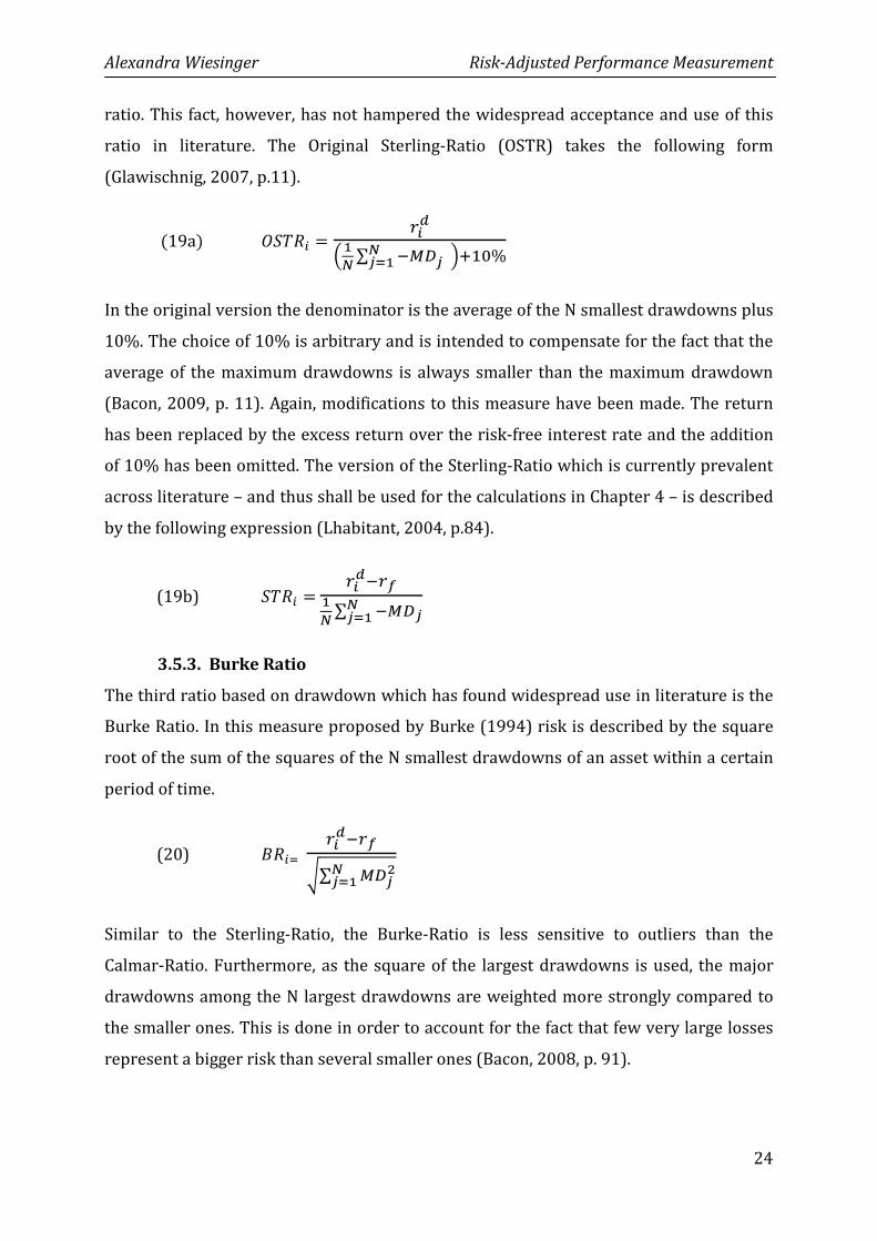
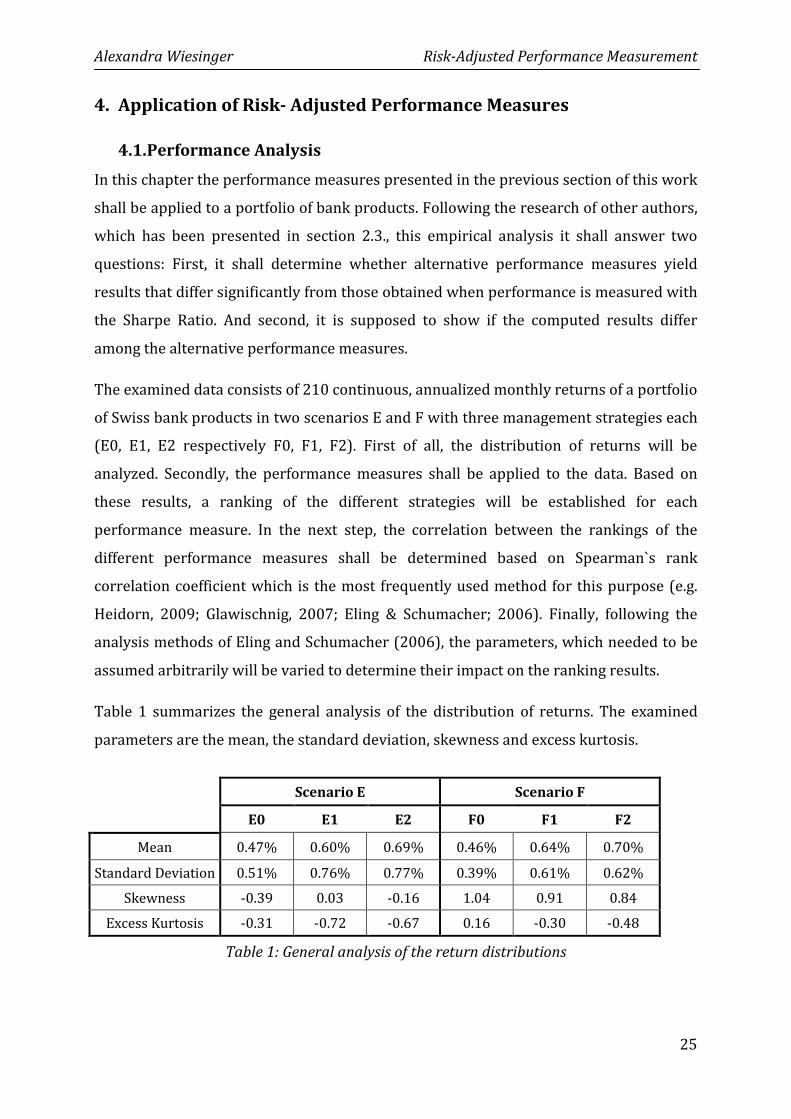
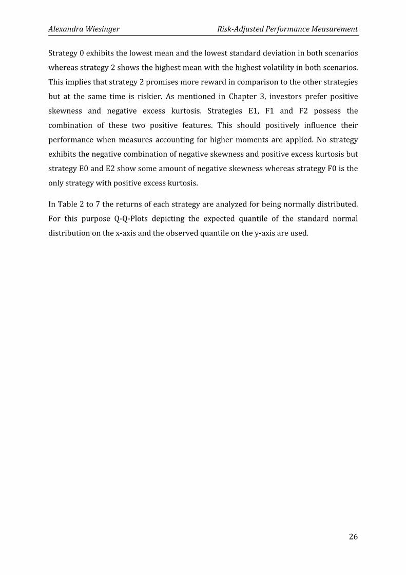
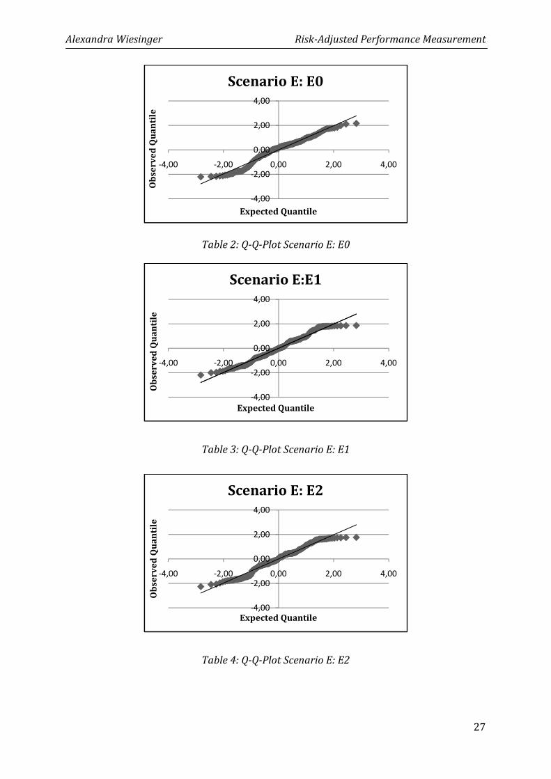
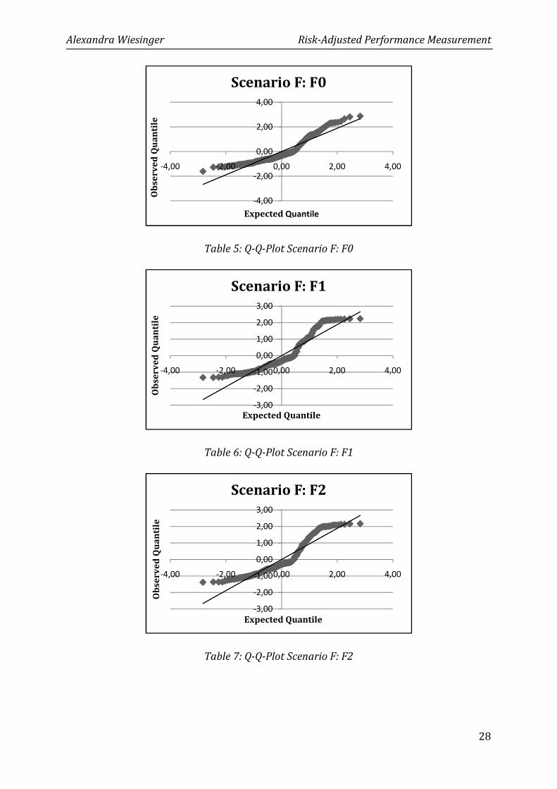
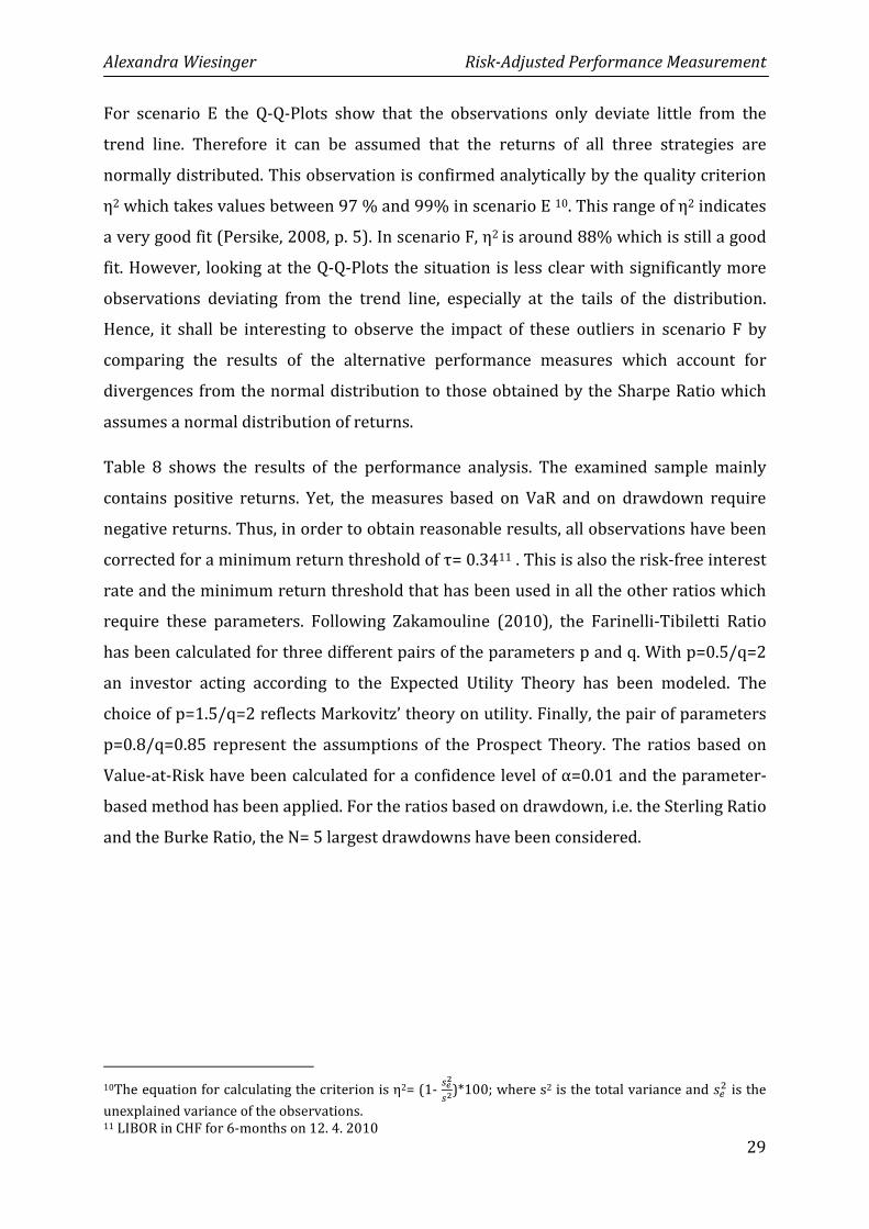
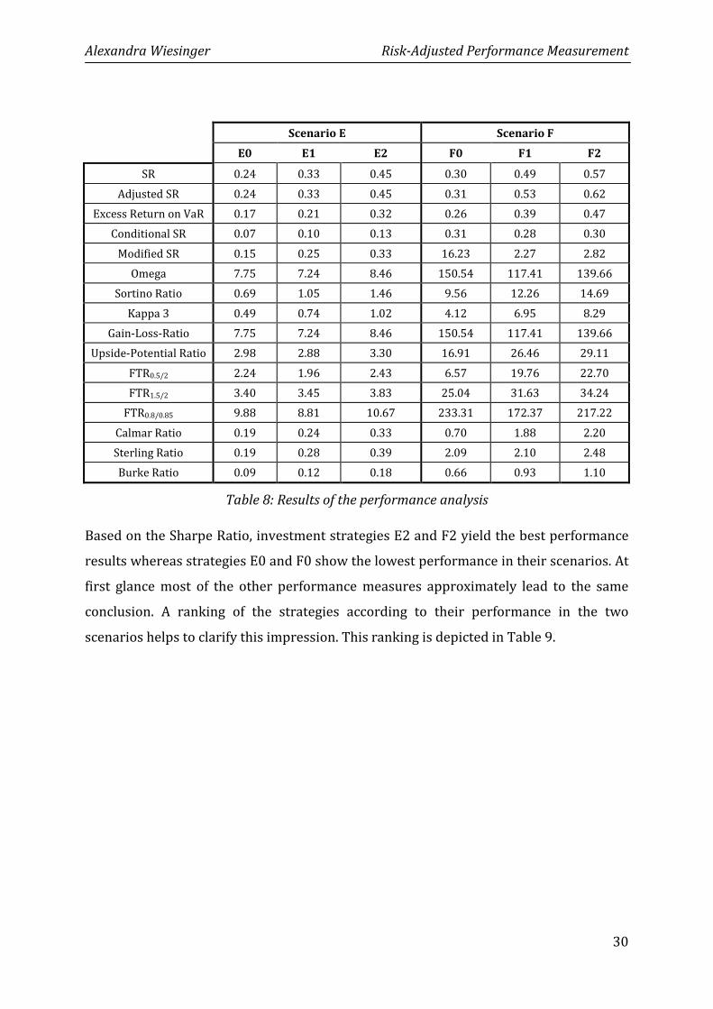
In Table 2 to 7 the returns of each strategy are analyzed for being normally distributed.
For this purpose Q-Q-Plots depicting the expected quantile of the standard normal
distribution on the x-axis and the observed quantile on the y-axis are used.
Alexandra Wiesinger Risk-Adjusted Performance Measurement
27
-4,00
-2,00
0,00
2,00
4,00
-4,00 -2,00 0,00 2,00 4,00
Ob
serv
ed
Qu
an
tile
Expected Quantile
Scenario E: E0
-4,00
-2,00
0,00
2,00
4,00
-4,00 -2,00 0,00 2,00 4,00
Ob
serv
ed
Qu
an
tile
Expected Quantile
Scenario E:E1
-4,00
-2,00
0,00
2,00
4,00
-4,00 -2,00 0,00 2,00 4,00
Ob
serv
ed
Qu
an
tile
Expected Quantile
Scenario E: E2
Table 4: Q-Q-Plot Scenario E: E2
Table 3: Q-Q-Plot Scenario E: E1
Table 2: Q-Q-Plot Scenario E: E0
Alexandra Wiesinger Risk-Adjusted Performance Measurement
28
Table 5: Q-Q-Plot Scenario F: F0
Table 6: Q-Q-Plot Scenario F: F1
Table 7: Q-Q-Plot Scenario F: F2
-4,00
-2,00
0,00
2,00
4,00
-4,00 -2,00 0,00 2,00 4,00
Ob
serv
ed
Qu
an
tile
Expected Quantile
Scenario F: F0
-3,00
-2,00
-1,00
0,00
1,00
2,00
3,00
-4,00 -2,00 0,00 2,00 4,00
Ob
serv
ed
Qu
an
tile
Expected Quantile
Scenario F: F1
-3,00
-2,00
-1,00
0,00
1,00
2,00
3,00
-4,00 -2,00 0,00 2,00 4,00
Ob
serv
ed
Qu
an
tile
Expected Quantile
Scenario F: F2
Alexandra Wiesinger Risk-Adjusted Performance Measurement
29
For scenario E the Q-Q-Plots show that the observations only deviate little from the
trend line. Therefore it can be assumed that the returns of all three strategies are
normally distributed. This observation is confirmed analytically by the quality criterion
η2 which takes values between 97 % and 99% in scenario E 10. This range of η2 indicates
a very good fit (Persike, 2008, p. 5). In scenario F, η2 is around 88% which is still a good
fit. However, looking at the Q-Q-Plots the situation is less clear with significantly more
observations deviating from the trend line, especially at the tails of the distribution.
Hence, it shall be interesting to observe the impact of these outliers in scenario F by
comparing the results of the alternative performance measures which account for
divergences from the normal distribution to those obtained by the Sharpe Ratio which
assumes a normal distribution of returns.
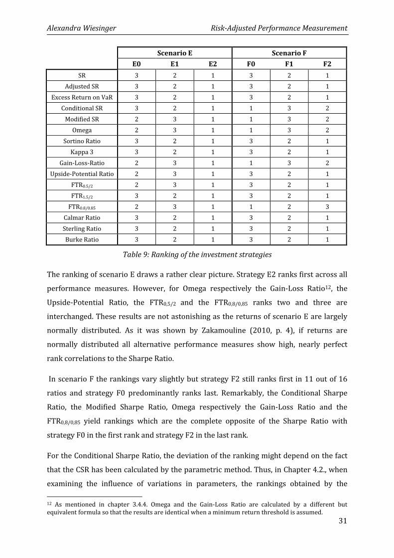
Table 8 shows the results of the performance analysis. The examined sample mainly
contains positive returns. Yet, the measures based on VaR and on drawdown require
negative returns. Thus, in order to obtain reasonable results, all observations have been
corrected for a minimum return threshold of τ= 0.3411 . This is also the risk-free interest
rate and the minimum return threshold that has been used in all the other ratios which
require these parameters. Following Zakamouline (2010), the Farinelli-Tibiletti Ratio
has been calculated for three different pairs of the parameters p and q. With p=0.5/q=2
an investor acting according to the Expected Utility Theory has been modeled. The
choice of p=1.5/q=2 reflects Markovitz’ theory on utility. Finally, the pair of parameters
p=0.8/q=0.85 represent the assumptions of the Prospect Theory. The ratios based on
Value-at-Risk have been calculated for a confidence level of α=0.01 and the parameter-
based method has been applied. For the ratios based on drawdown, i.e. the Sterling Ratio
and the Burke Ratio, the N= 5 largest drawdowns have been considered.
10The equation for calculating the criterion is η2= (1-
��s�s)*100; where s2 is the total variance and ��& is the
unexplained variance of the observations. 11 LIBOR in CHF for 6-months on 12. 4. 2010
Alexandra Wiesinger Risk-Adjusted Performance Measurement
30
Scenario E Scenario F
E0 E1 E2 F0 F1 F2
SR 0.24 0.33 0.45 0.30 0.49 0.57
Adjusted SR 0.24 0.33 0.45 0.31 0.53 0.62
Excess Return on VaR 0.17 0.21 0.32 0.26 0.39 0.47
Conditional SR 0.07 0.10 0.13 0.31 0.28 0.30
Modified SR 0.15 0.25 0.33 16.23 2.27 2.82
Omega 7.75 7.24 8.46 150.54 117.41 139.66
Sortino Ratio 0.69 1.05 1.46 9.56 12.26 14.69
Kappa 3 0.49 0.74 1.02 4.12 6.95 8.29
Gain-Loss-Ratio 7.75 7.24 8.46 150.54 117.41 139.66
Upside-Potential Ratio 2.98 2.88 3.30 16.91 26.46 29.11
FTR0.5/2 2.24 1.96 2.43 6.57 19.76 22.70
FTR1.5/2 3.40 3.45 3.83 25.04 31.63 34.24
FTR0.8/0.85 9.88 8.81 10.67 233.31 172.37 217.22
Calmar Ratio 0.19 0.24 0.33 0.70 1.88 2.20
Sterling Ratio 0.19 0.28 0.39 2.09 2.10 2.48
Burke Ratio 0.09 0.12 0.18 0.66 0.93 1.10
Table 8: Results of the performance analysis
Based on the Sharpe Ratio, investment strategies E2 and F2 yield the best performance
results whereas strategies E0 and F0 show the lowest performance in their scenarios. At
first glance most of the other performance measures approximately lead to the same
conclusion. A ranking of the strategies according to their performance in the two
scenarios helps to clarify this impression. This ranking is depicted in Table 9.
Alexandra Wiesinger Risk-Adjusted Performance Measurement
31
Scenario E Scenario F
E0 E1 E2 F0 F1 F2
SR 3 2 1 3 2 1
Adjusted SR 3 2 1 3 2 1
Excess Return on VaR 3 2 1 3 2 1
Conditional SR 3 2 1 1 3 2
Modified SR 2 3 1 1 3 2
Omega 2 3 1 1 3 2
Sortino Ratio 3 2 1 3 2 1
Kappa 3 3 2 1 3 2 1
Gain-Loss-Ratio 2 3 1 1 3 2
Upside-Potential Ratio 2 3 1 3 2 1
FTR0.5/2 2 3 1 3 2 1
FTR1.5/2 3 2 1 3 2 1
FTR0.8/0.85 2 3 1 1 2 3
Calmar Ratio 3 2 1 3 2 1
Sterling Ratio 3 2 1 3 2 1
Burke Ratio 3 2 1 3 2 1
Table 9: Ranking of the investment strategies
The ranking of scenario E draws a rather clear picture. Strategy E2 ranks first across all
performance measures. However, for Omega respectively the Gain-Loss Ratio12, the
Upside-Potential Ratio, the FTR0,5/2 and the FTR0,8/0,85 ranks two and three are
interchanged. These results are not astonishing as the returns of scenario E are largely
normally distributed. As it was shown by Zakamouline (2010, p. 4), if returns are
normally distributed all alternative performance measures show high, nearly perfect
rank correlations to the Sharpe Ratio.
In scenario F the rankings vary slightly but strategy F2 still ranks first in 11 out of 16
ratios and strategy F0 predominantly ranks last. Remarkably, the Conditional Sharpe
Ratio, the Modified Sharpe Ratio, Omega respectively the Gain-Loss Ratio and the
FTR0,8/0,85 yield rankings which are the complete opposite of the Sharpe Ratio with
strategy F0 in the first rank and strategy F2 in the last rank.
For the Conditional Sharpe Ratio, the deviation of the ranking might depend on the fact
that the CSR has been calculated by the parametric method. Thus, in Chapter 4.2., when
examining the influence of variations in parameters, the rankings obtained by the
12 As mentioned in chapter 3.4.4. Omega and the Gain-Loss Ratio are calculated by a different but
equivalent formula so that the results are identical when a minimum return threshold is assumed.
Alexandra Wiesinger Risk-Adjusted Performance Measurement
32
parametric method should be compared to the rankings which result when the
Conditional Value-at-Risk is calculated with the empirical method in order to verify if
the difference to the Sharpe Ratio depends on the applied method.
For the Modified Sharpe Ratio the driver of the different ranking results compared to the
Sharpe Ratio is mainly skewness. Strategy F0 has the highest positive skewness in
scenario F, which leads to a lower Modified Value-at-Risk as in this ratio positive
skewness is rewarded. As a result strategy F0 possesses the highest value for the
Modified Sharpe Ratio. As strategy F2 has the lowest positive skewness of all strategies
in scenario F, it also yields the lowest Modified Sharpe Ratio and therefore ranks last.
The explanation for the inverted ranking of Omega respectively the Gain-Loss Ratio and
the FTR0.8/0.85 is not that clear at first sight. As both ratios largely depend on the
assumed return threshold the ranking may change if the return threshold is changed.
This hypothesis shall be investigated further in Chapter 4.2. when the underlying
parameters are varied.
The overall results of the rankings for scenario E in Table 9 suggest that the rankings
obtained by the respective performance measures are to a large extent the same which
is explained by the largely normally distributed returns of scenario E. In scenario F the
rankings are the same for the majority of performance measures but with significant
exceptions. To support these observations analytically, the correlation of the ranks was
calculated using Spearman’s rank correlation coefficient ρ. It is calculated by the
following formula (Zöfel, 2000, p. 127).
(21) � = 1 � 6 ∑ DC2¡C=1¡3�¡
d …… difference between the ranks of each observation
n …….. number of observations

Alexandra Wiesinger Risk-Adjusted Performance Measurement
33
The results of this analysis are shown in Table 10 for scenario E and in Table 11 for
scenario F.
Sh
arp
e R
ati
o
Ad
just
ed
SR
EV
aR
Co
nd
itio
na
l S
R
Mo
dif
ied
SR
Om
eg
a
So
rtin
o R
ati
o
Ka
pp
a 3
GL
R
UP
R
FT
R0
.5/
2
FT
R1
.5/
2
FT
R0
.8/
0.8
5
Ca
lma
r R
ati
o
Ste
rlin
g R
ati
o
Bu
rke
Ra
tio
Sharpe Ratio
Adjusted SR 1.00
EVaR 1.00 1.00
CSR 1.00 1.00 1.00
Modified SR 1.00 1.00 1.00 1.00
Omega 0.92 0.92 0.92 0.92 0.92
Sortino Ratio 1.00 1.00 1.00 1.00 1.00 0.92
Kappa 3 1.00 1.00 1.00 1.00 1.00 0.92 1.00
GLR 0.92 0.92 0.92 0.92 0.92 1.00 0.92 0.92
UPR 0.92 0.92 0.92 0.92 0.92 1.00 0.92 0.92 1.00
FTR0.5/2 0.92 0.92 0.92 0.92 0.92 1.00 0.92 0.92 1.00 1.00
FTR1.5/2 1.00 1.00 1.00 1.00 1.00 0.92 1.00 1.00 0.92 0.92 0.92
FTR0.8/0.85 0.92 0.92 0.92 0.92 0.92 1.00 0.92 0.92 1.00 1.00 1.00 0.92
Calmar Ratio 1.00 1.00 1.00 1.00 1.00 0.92 1.00 1.00 0.92 0.92 0.92 1.00 0.92
Sterling Ratio 1.00 1.00 1.00 1.00 1.00 0.92 1.00 1.00 0.92 0.92 0.92 1.00 0.92 1.00
Burke Ratio 1.00 1.00 1.00 1.00 1.00 0.92 1.00 1.00 0.92 0.92 0.92 1.00 0.92 1.00 1.00
Average 0.97 0.97 0.97 0.97 0.95 0.97 0.97 0.94 0.95 0.94 0.93 0.94 0.96 0.97 0.97 0.97
Table 10: Rank correlations for scenario E
In general, all performance measures show high rank correlations to the Sharpe Ratio
and to each other. As indicated above, the picture in scenario E is very clear with all
ratios being perfectly correlated to the Sharpe Ratio except for Omega resp. the Gain-
Loss Ratio and the Upside-Potential Ratio. The average rank correlation to the Sharpe
Ratio in scenario E is 0.97. Comparing the alternative performance measures to each
other, the lowest ranking coefficient is 0.92. This results if ranks 2 and 3 are
interchanged in some measures. The total average of all ranking coefficients is 0.96.
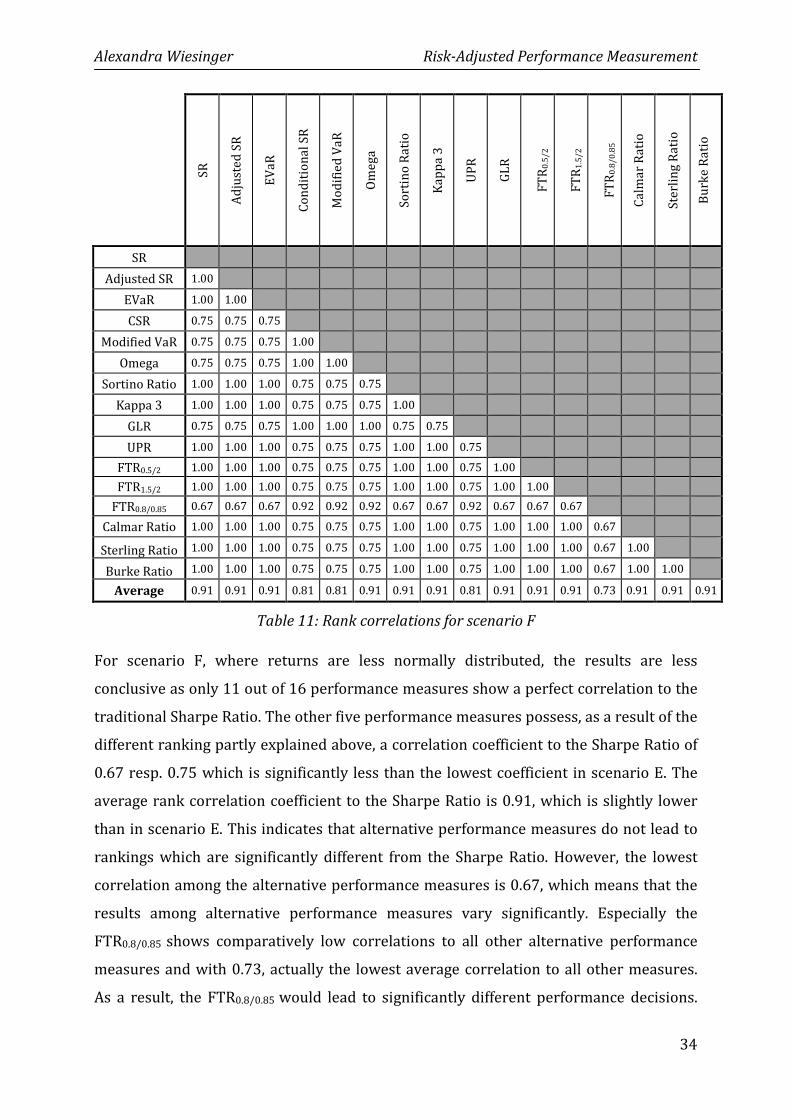
Alexandra Wiesinger Risk-Adjusted Performance Measurement
34
SR
Ad
just
ed
SR
EV
aR
Co
nd
itio
na
l S
R
Mo
dif
ied
Va
R
Om
eg
a
So
rtin
o R
ati
o
Ka
pp
a 3
UP
R
GL
R
FT
R0
.5/
2
FT
R1
.5/
2
FT
R0
.8/
0.8
5
Ca
lma
r R
ati
o
Ste
rlin
g R
ati
o
Bu
rke
Ra
tio
SR
Adjusted SR 1.00
EVaR 1.00 1.00
CSR 0.75 0.75 0.75
Modified VaR 0.75 0.75 0.75 1.00
Omega 0.75 0.75 0.75 1.00 1.00
Sortino Ratio 1.00 1.00 1.00 0.75 0.75 0.75
Kappa 3 1.00 1.00 1.00 0.75 0.75 0.75 1.00
GLR 0.75 0.75 0.75 1.00 1.00 1.00 0.75 0.75
UPR 1.00 1.00 1.00 0.75 0.75 0.75 1.00 1.00 0.75
FTR0.5/2 1.00 1.00 1.00 0.75 0.75 0.75 1.00 1.00 0.75 1.00
FTR1.5/2 1.00 1.00 1.00 0.75 0.75 0.75 1.00 1.00 0.75 1.00 1.00
FTR0.8/0.85 0.67 0.67 0.67 0.92 0.92 0.92 0.67 0.67 0.92 0.67 0.67 0.67
Calmar Ratio 1.00 1.00 1.00 0.75 0.75 0.75 1.00 1.00 0.75 1.00 1.00 1.00 0.67
Sterling Ratio 1.00 1.00 1.00 0.75 0.75 0.75 1.00 1.00 0.75 1.00 1.00 1.00 0.67 1.00
Burke Ratio 1.00 1.00 1.00 0.75 0.75 0.75 1.00 1.00 0.75 1.00 1.00 1.00 0.67 1.00 1.00
Average 0.91 0.91 0.91 0.81 0.81 0.91 0.91 0.91 0.81 0.91 0.91 0.91 0.73 0.91 0.91 0.91
Table 11: Rank correlations for scenario F
For scenario F, where returns are less normally distributed, the results are less
conclusive as only 11 out of 16 performance measures show a perfect correlation to the
traditional Sharpe Ratio. The other five performance measures possess, as a result of the
different ranking partly explained above, a correlation coefficient to the Sharpe Ratio of
0.67 resp. 0.75 which is significantly less than the lowest coefficient in scenario E. The
average rank correlation coefficient to the Sharpe Ratio is 0.91, which is slightly lower
than in scenario E. This indicates that alternative performance measures do not lead to
rankings which are significantly different from the Sharpe Ratio. However, the lowest
correlation among the alternative performance measures is 0.67, which means that the
results among alternative performance measures vary significantly. Especially the
FTR0.8/0.85 shows comparatively low correlations to all other alternative performance
measures and with 0.73, actually the lowest average correlation to all other measures.
As a result, the FTR0.8/0.85 would lead to significantly different performance decisions.
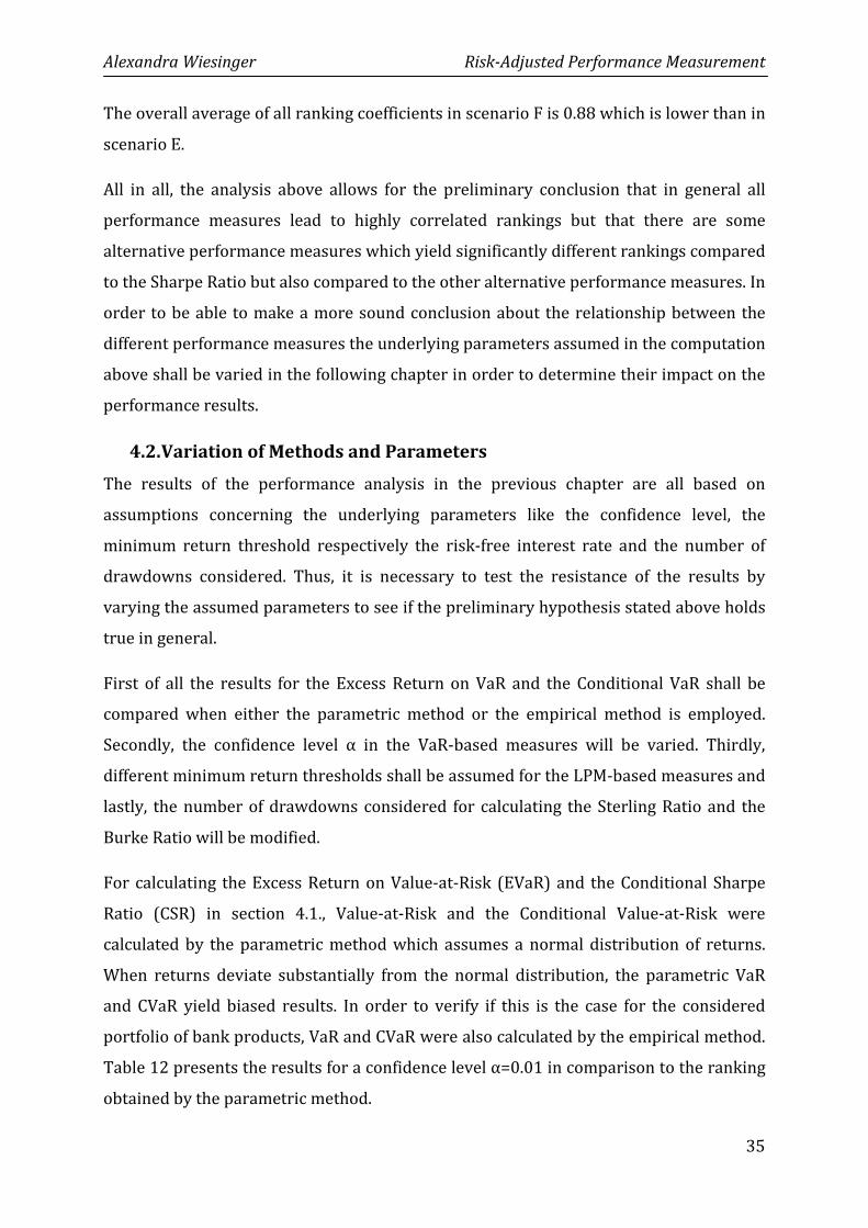
Alexandra Wiesinger Risk-Adjusted Performance Measurement
35
The overall average of all ranking coefficients in scenario F is 0.88 which is lower than in
scenario E.
All in all, the analysis above allows for the preliminary conclusion that in general all
performance measures lead to highly correlated rankings but that there are some
alternative performance measures which yield significantly different rankings compared
to the Sharpe Ratio but also compared to the other alternative performance measures. In
order to be able to make a more sound conclusion about the relationship between the
different performance measures the underlying parameters assumed in the computation
above shall be varied in the following chapter in order to determine their impact on the
performance results.
4.2. Variation of Methods and Parameters
The results of the performance analysis in the previous chapter are all based on
assumptions concerning the underlying parameters like the confidence level, the
minimum return threshold respectively the risk-free interest rate and the number of
drawdowns considered. Thus, it is necessary to test the resistance of the results by
varying the assumed parameters to see if the preliminary hypothesis stated above holds
true in general.
First of all the results for the Excess Return on VaR and the Conditional VaR shall be
compared when either the parametric method or the empirical method is employed.
Secondly, the confidence level α in the VaR-based measures will be varied. Thirdly,
different minimum return thresholds shall be assumed for the LPM-based measures and
lastly, the number of drawdowns considered for calculating the Sterling Ratio and the
Burke Ratio will be modified.
For calculating the Excess Return on Value-at-Risk (EVaR) and the Conditional Sharpe
Ratio (CSR) in section 4.1., Value-at-Risk and the Conditional Value-at-Risk were
calculated by the parametric method which assumes a normal distribution of returns.
When returns deviate substantially from the normal distribution, the parametric VaR
and CVaR yield biased results. In order to verify if this is the case for the considered
portfolio of bank products, VaR and CVaR were also calculated by the empirical method.
Table 12 presents the results for a confidence level α=0.01 in comparison to the ranking
obtained by the parametric method.
Alexandra Wiesinger Risk-Adjusted Performance Measurement
36
Scenario E Scenario F
E0 E1 E2 F0 F1 F2
SR 3 2 1 3 2 1
Parametric EVaR 3 2 1 3 2 1
Empirical EVaR 3 2 1 1 3 2
Parametric CSR 3 2 1 1 3 2
Empirical CSR 3 2 1 3 2 1
Table 12: Parametric vs. Empirical EVaR and CSR
In scenario E it does not make a difference whether the Parametric or the Empirical VaR
and CVaR are employed. Both methods and both performance measures lead to the
same rankings. And those rankings coincide with the rankings obtained when using the
traditional Sharpe Ratio (SR).
In scenario F, however, the empirical and the parametric method yield the reversed
ranking for both performance measures. For the Empirical EVaR the resulting ranking is
completely contrary to the ranking obtained by using the Sharpe Ratio, whereas the
Empirical CSR leads to exactly the same ranking as the Sharpe Ratio. This supports the
assumption made in section 4.1., that the opposing ranking of the CSR is a result of the
applied calculation method. As the empirical and parametric method yield significantly
different results for scenario F, the empirical method should be used to calculate VaR
and CVaR whenever there is enough empirical data available in order to obtain exact
results.
So far, a confidence level of α=0.01 was assumed for the VaR- based performance
measures Exess Return on VaR, Conditional Sharpe Ratio and Modified Sharpe Ratio. In
order to test the resistance of the results, the confidence levels were varied from α=0.01
to α=0.1 in order to examine their impact on the performance results. The rankings for
different confidence levels are summarized in Table 13.
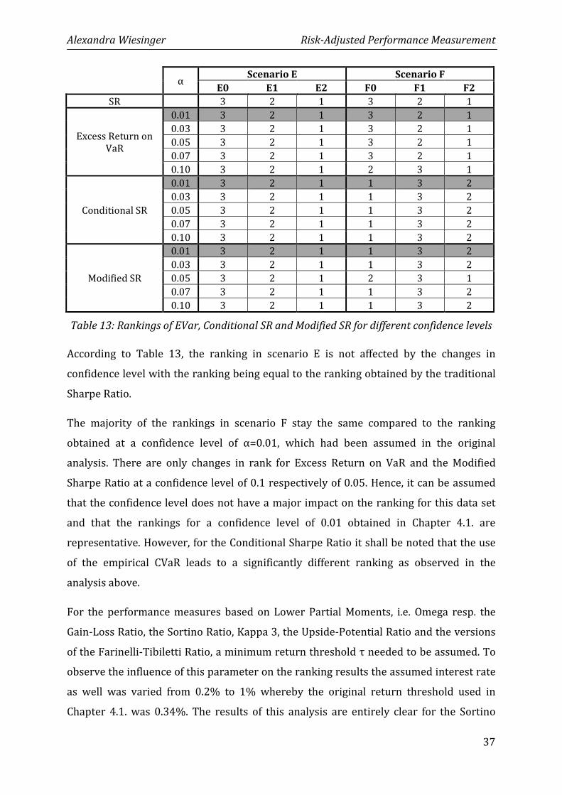
Alexandra Wiesinger Risk-Adjusted Performance Measurement
37
α Scenario E Scenario F
E0 E1 E2 F0 F1 F2
SR 3 2 1 3 2 1
Excess Return on
VaR
0.01 3 2 1 3 2 1
0.03 3 2 1 3 2 1
0.05 3 2 1 3 2 1
0.07 3 2 1 3 2 1
0.10 3 2 1 2 3 1
Conditional SR
0.01 3 2 1 1 3 2
0.03 3 2 1 1 3 2
0.05 3 2 1 1 3 2
0.07 3 2 1 1 3 2
0.10 3 2 1 1 3 2
Modified SR
0.01 3 2 1 1 3 2
0.03 3 2 1 1 3 2
0.05 3 2 1 2 3 1
0.07 3 2 1 1 3 2
0.10 3 2 1 1 3 2
Table 13: Rankings of EVar, Conditional SR and Modified SR for different confidence levels
According to Table 13, the ranking in scenario E is not affected by the changes in
confidence level with the ranking being equal to the ranking obtained by the traditional
Sharpe Ratio.
The majority of the rankings in scenario F stay the same compared to the ranking
obtained at a confidence level of α=0.01, which had been assumed in the original
analysis. There are only changes in rank for Excess Return on VaR and the Modified
Sharpe Ratio at a confidence level of 0.1 respectively of 0.05. Hence, it can be assumed
that the confidence level does not have a major impact on the ranking for this data set
and that the rankings for a confidence level of 0.01 obtained in Chapter 4.1. are
representative. However, for the Conditional Sharpe Ratio it shall be noted that the use
of the empirical CVaR leads to a significantly different ranking as observed in the
analysis above.
For the performance measures based on Lower Partial Moments, i.e. Omega resp. the
Gain-Loss Ratio, the Sortino Ratio, Kappa 3, the Upside-Potential Ratio and the versions
of the Farinelli-Tibiletti Ratio, a minimum return threshold τ needed to be assumed. To
observe the influence of this parameter on the ranking results the assumed interest rate
as well was varied from 0.2% to 1% whereby the original return threshold used in
Chapter 4.1. was 0.34%. The results of this analysis are entirely clear for the Sortino
Alexandra Wiesinger Risk-Adjusted Performance Measurement
38
Ratio and Kappa 3 and the Upside-Potential Ratio with no changes in ranking for the
whole range of assumed interest rates.13 So the rankings of the Sortino Ratio, Kappa 3
and the Upside-Potential Ratio coincide with the ranking of the traditional Sharpe Ratio
for all assumed interest rates except for a minor deviation of rank two and three in the
Upside-Potential Ratio in scenario E.
The ranking for different interest rates for Omega respectively the Gain-Loss Ratio and
the versions of the Farinelli-Tibiletti Ratio, however, give interesting insights and are
depicted in Table 14.
13 As there are no changes in ranking, the results for Omega, the Sortino Ratio and Kappa 3 shall not be
presented separately at this point of the work. For the detailed results of the variation of interest rates and
number of drawdowns please see the Appendix.
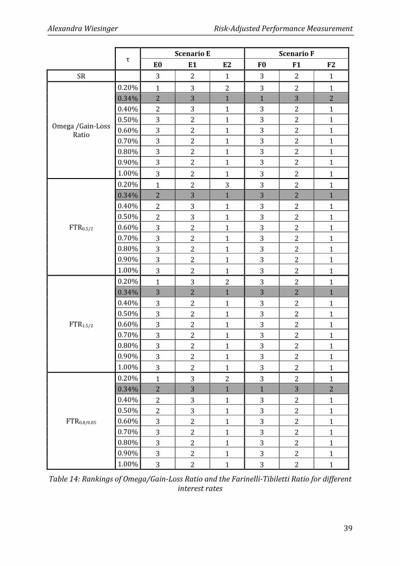
Alexandra Wiesinger Risk-Adjusted Performance Measurement
39
τ Scenario E Scenario F
E0 E1 E2 F0 F1 F2
SR 3 2 1 3 2 1
Omega /Gain-Loss
Ratio
0.20% 1 3 2 3 2 1
0.34% 2 3 1 1 3 2
0.40% 2 3 1 3 2 1
0.50% 3 2 1 3 2 1
0.60% 3 2 1 3 2 1
0.70% 3 2 1 3 2 1
0.80% 3 2 1 3 2 1
0.90% 3 2 1 3 2 1
1.00% 3 2 1 3 2 1
FTR0.5/2
0.20% 1 2 3 3 2 1
0.34% 2 3 1 3 2 1
0.40% 2 3 1 3 2 1
0.50% 2 3 1 3 2 1
0.60% 3 2 1 3 2 1
0.70% 3 2 1 3 2 1
0.80% 3 2 1 3 2 1
0.90% 3 2 1 3 2 1
1.00% 3 2 1 3 2 1
FTR1.5/2
0.20% 1 3 2 3 2 1
0.34% 3 2 1 3 2 1
0.40% 3 2 1 3 2 1
0.50% 3 2 1 3 2 1
0.60% 3 2 1 3 2 1
0.70% 3 2 1 3 2 1
0.80% 3 2 1 3 2 1
0.90% 3 2 1 3 2 1
1.00% 3 2 1 3 2 1
FTR0.8/0.85
0.20% 1 3 2 3 2 1
0.34% 2 3 1 1 3 2
0.40% 2 3 1 3 2 1
0.50% 2 3 1 3 2 1
0.60% 3 2 1 3 2 1
0.70% 3 2 1 3 2 1
0.80% 3 2 1 3 2 1
0.90% 3 2 1 3 2 1
1.00% 3 2 1 3 2 1
Table 14: Rankings of Omega/Gain-Loss Ratio and the Farinelli-Tibiletti Ratio for different interest rates
Alexandra Wiesinger Risk-Adjusted Performance Measurement
40
As indicated in Chapter 4.1., Omega resp. the Gain-Loss Ratio, the FTR0.5/2 and the FTR0.8/0.85
were among the few ratios in scenario E which did not comply with the ranking of the
traditional Sharpe Ratio. In scenario F some of these ratios even led to an inverted
ranking compared to the Sharpe Ratio. Table 14 shows that the rankings produced by
these four performance measures vary significantly for small interest rates (up to 0.5%)
For higher interest rates the rankings are stable and coincide with the ranking produced
by the Sharpe Ratio. Thus, the influence of the interest rate may not be neglected as it
might lead to significantly different investment decisions when small values of τ are
chosen.
The last parameter which needs to be varied and examined is the number of drawdowns
used in the Sterling Ratio and in the Burke Ratio. In the original analysis in Chapter 4.1.
the number of drawdowns considered was N=5. To test the resistance of the results the
number of drawdowns was varied from N= 2 to N=10. The results show a very clear
picture as the ranking in both ratios does not change at all for both scenarios when the
number of drawdowns is altered so that the ranking of the Sterling and the Burke Ratio
corresponds to the ranking of the traditional Sharpe Ratio for each number of
drawdowns observed14.
Summarizing the variations in methods and parameters, it can be stated that the results
have proven to be relatively resistant against changes of the underlying parameters,
especially considering the confidence level and the number of drawdowns. The change
in the computation method of VaR and CVaR, however, led to significant differences in
ranks. The same applies to the variation of the interest rate for Omega resp. the Gain-
Loss Ratio and the versions of the Farinelli-Tibiletti Ratio when small values for the
interest rate were chosen.
Both the original performance analysis and the variation of parameters and methods
confirm the preliminary conclusion stated above that – in general – risk-adjusted
performance measures produce highly correlated rankings. But some performance
measures produce significantly different rankings compared to the Sharpe Ratio and to
other alternative performance measures. Furthermore, the computation method and the
14 For the exact results please see the Appendix.
Alexandra Wiesinger Risk-Adjusted Performance Measurement
41
choice of interest rate under certain circumstances have a significant influence on the
ranking results for some performance measures. Thus, based on the analysis of bank
products in this work, it seems hasty to dismiss alternative performance measures
which account for higher moments of distributions and to declare performance
measurement with the Sharpe Ratio to be sufficient as it was done by Eling and
Schumacher (2006).
The author of this work agrees with the argumentation of Glawischnig (2007, p. 27)
which states that the information contained in the higher moments of distributions
needs to be considered even if it does not lead to significantly different rankings for
most performance measures. The reason for this is that, as shown in the empirical
analysis above, there are some performance measures and some calibrations of
parameters that lead to differences in rankings which might be important to a particular
investor. Moreover, the choice between different performance measures, despite
producing similar results in many cases, helps the investor to find a performance
measure which exactly reflects his preferences and thus leads to an optimal decision
from his point of view (Bacon, 2009, p. 12).
Alexandra Wiesinger Risk-Adjusted Performance Measurement
42
5. Conclusion
Risk-adjusted performance measures can take many forms and their main fields of
application lie within performance evaluation of investment strategies and efficient
internal capital allocation especially in financial institutions. The selection of the in the
scientific literature most frequently applied and discussed risk-adjusted performance
measures presented in Chapter 3 was categorized according to the risk-measure used in
the respective ratios. The categories are performance measures based on volatility,
Value-at Risk, Lower Partial Moments and drawdown. The Sharpe Ratio, Excess Return
on Value-at Risk and the Conditional Sharpe Ratio in its parametric forms assume
normally distributed returns. All other measures try to overcome this strong assumption
by explicitly or implicitly considering the information contained in the higher moments
of distributions.
To verify whether alternative performance measures lead to significantly different
investment decisions than the Sharpe Ratio and other performance measures which
assume normally distributed returns, the presented ratios have been applied to a
portfolio of bank products. The analysis of the results has shown that both traditional
and alternative performance ratios produce highly correlated rankings. As the results
strongly depend on the underlying parameters, like the minimum return threshold, the
resistance of the results was tested. This was done by altering the calculation method of
Value-at-Risk and Conditional Value-at-Risk, the confidence level, the minimum return
threshold and the number of drawdowns. The analysis shows that the performance
results in general are not very sensitive to changes especially in confidence level and in
the number of drawdowns considered and thus, in general lead to the same rankings.
Different computation methods for VaR and CVaR and low values for the interest rate,
however, lead to significant changes in rankings for some performance measures.
These findings support the conclusion of other authors that risk-adjusted performance
measurement based on the Sharpe Ratio only is not sufficient and that alternative
performance measures deliver additional, important information for investment
decisions. Still, as it was the case in studies conducted in the current literature of
performance analysis, the analysis conducted in this work cannot tell exactly which
performance measures under which circumstances and for what reasons lead to
different performance results compared to the Sharpe Ratio and to each other. So far all
studies, including this work, were based on a rather small selection of performance
measures and asset classes. This is why the conclusions derived so far might only be of

Alexandra Wiesinger Risk-Adjusted Performance Measurement
43
limited general validity. A study which covers all alternatives to the Sharpe Ratio based
on a broad range of asset classes seems an enormous task as there are more than 100
performance measures identified in literature (Cogneau & Hübner, 2010). Yet, it seems
to be the only way to bring more transparency into the existing discussion concerning
traditional and alternative risk-adjusted performance measures.
Alexandra Wiesinger Risk-Adjusted Performance Measurement
44
References
Acerbi, C. & Tasche, D. (2002). On the Coherence of Expected Shortfall. Journal of
Banking and Finance, 26, 1486- 1503.
Agarwal, V. & Naik, N.Y. (2004). Risk and portfolio decisions involving hedge funds.
Review of Financial Studies, 17(1), 63–98.
Albrecht, P. & Koryciorz, S. (2003). Bestimmung des Conditional Value-at-Risk bei
Normal- bzw. Lognormalverteilung. Mannheimer Manuskripte zur Risikotheorie,
Portfolio Management und Versicherungswirtschaft Nr. 142.
Aparicio, F. & Estrada J. (2001). Empirical distributions of stock returns: European
securities markets 1990-95. The European Journal of Finance, 7, 1-21.
Artzner, P., Delbaen, F., Eber, J.M. & Heath, D. (1997). Thinking coherently. Risk
Magazine, 10(11), 68-71.
Bacon. C. (2008). Practical Performance Measurement and Attribution. New York: John
Wiley & Sons.
Bacon, C. (2009). How Sharp is the Sharpe Ratio. Statpro Whitepaper. Retrieved on 25
February 2010 from
http://www.statpro.com/resources/whitepapers/how_sharp_is_the_sharp_ratio.a
spx
Beder, T. (1995). VAR: Seductive but Dangerous. Financial Analysts Journal, 51(5), 12-24.
Bernardo, A.E. & Ledoit, O. (2000). Gain, loss and asset pricing. Journal of Political
Economy, 108(1), 144–172.
Brooks, C. & Kat, H.M. (2002). The statistical properties of hedge fund index returns and
their implications for investors. Journal of Alternative Investments, 5(2), 26–44.
Bürkler, N. & Hunziker S. (2008). Rendite, Risiko und Performance – eine Übersicht. IFZ
Working Paper 003/2008.
Burke, G. (1994). A Sharper Sharpe Ratio. Futures, 23(3), 56-57.
Alexandra Wiesinger Risk-Adjusted Performance Measurement
45
Cogneau, P. & Hübner, G. (2009). 101 Ways to Measure Portfolio Performance. Working
Paper. Ecole de Gestion de l’Université de Liège. Retrieved on 12 April 2010 from
http://www.hec.ulg.ac.be/FR/recherche/activites/working-
papers/documents/WP_HECULg_20090201_Cogneau_Hubner.pdf
Dowd, K. (2000). Adjusting for Risk: An Improved Sharpe Ratio. International Review of
Economics and Finance, 9(3), S. 209-222.
Eisele, B. (2004). Value-at-Risk-basiertes Risikomanagement in Banken. Wiesbaden:
Gabler.
Ekholm, A. & Pasternack, D. (2005). The negative news threshold – an explanation for
negative Skewness in stock returns. The European Journal of Finance, 11, 511–529.
Eling M. & Schumacher F. (2006): Hat die Wahl des Performancemaßes einen Einfluss
auf die Beurteilung von Hedgefondsindizes?, Kredit und Kapital, 39(3), 419-457.
Embrechts, P. (2000). Extreme Value Theory: Potential and Limitations as an Integrated
Risk Management Tool. Derivatives Use, Trading & Regulation, 6, 449-456.
Farinelli, S. & Tibiletti, L. (2008). Sharpe Thinking in Asset Ranking with One-Sided
Measures. European Journal of Operational Research, 185(3), 1542–1547.
Favre L. & Galeano J. (2002). Mean-modified value at risk optimization with hedge funds.
Journal of Alternative Investment, 5, 1-11.
Forsey, H. (2001). The Mathematician’s View: Modelling Uncertainty with the Three
Parameter Lognormal. In Sortino, F. & Satchell, S. (Eds). Managing Downside Risk in
Financial Markets (p. 51-58). Oxford: Reed Educational and Professional
Publishing.
Glawischnig, M. (2007). Hedge Fonds Indizes: Unterschiede zwischen klassischen und
alternativen Performance- und Risikomassen. Institut fur Finanzwirtschaft, Karl-
Franzens Universität Graz.
Gregoriou G. & Gueyie J. (2003). Risk-Adjusted Performance of Funds of Hedge Funds
Using a Modified Sharpe Ratio. The Journal of Alternative Investments, 6(3), 77-83.
Alexandra Wiesinger Risk-Adjusted Performance Measurement
46
Guse, F. & Rudolf, M. (2008). Schiefe in der Portfolio-Selektion. Kredit und Kapital, 41(2),
197- 216.
Heidorn, M. (2009). Hedge Fund Performance Evaluation – Does Choice Matter? Research
Paper presented at the Midwest Finance Association 2010. Retrieved on 4 April
2010 from
http://www.mfa-2010.com/papers/HF%20Performance%20Evaluation.pdf
Hodges, S. (1998). A generalization of the Sharpe ratio and its applications to valuation
bounds and risk measures. Working Paper, Financial Options Research Centre,
University of Warwick.
Ingersoll, J., Spiegel, M. & Goetzmann, W.(2007). Portfolio performance manipulation
and manipulation-proof performance measures. Review of Financial Studies, 20(5),
1503–1546.
Jorion, P. (2006). Value at Risk. (3rd Ed.). Singapore, McGraw-Hill.
Kahneman, D. & Tversky, A. (1979). Prospect Theory: An Analysis of Decision Under
Risk. Econometrica, 47(12), 263–291.
Kaiser, D.G., Heidorn, T. & Roder, C. (2009). Empirische Analyse der Drawdowns von
Dach-Hedgefonds. Frankfurt School of Finance & Management. Working Paper
Series No. 109.
Kaplan, P. & Knowles, J. (2004). Kappa: A Generalized Downside Risk-Adjusted
Performance Measure. Journal of Performance Measurement, 8(3), 42-54.
Kazemi, H., Schneeweis, T. & Gupta, B. (2004). Omega as a Performance Measure. Journal
of Performance Measurement, Spring 2004.
Kosowski, R., Naik, N. & Teo, M. (2007). Do hedge funds deliver alpha? A Bayesian
andbootstrap analysis. Journal of Financial Economics, 84, 229–264.
Kremer, J. (2008). Value-at-Risk und kohärente Risikomaße. Berlin: Springer.
Leland, H.E. (1999). Beyond mean-variance: Risk and performance measurement in a
nonsymmetrical world. Financial Analysts Journal, 1, 27–36.
Alexandra Wiesinger Risk-Adjusted Performance Measurement
47
Lister, M. (1997). Risikoadjustierte Ergebnismessung und Risikokapitalallokation.
Frankfurt a. M.: Fritz Knapp Verlag.
Malkiel, B.G. & Saha, A. (2005). Hedge funds: Risk and return. Financial Analysts Journal
61(6), 80-88.
Mandelbrot. B. (1963) The variation of certain speculative prices. Journal of Business, 36,
394-419.
Markowitz, H. (1952). The Utility of Wealth. Journal of Political Economy, 6 (2), 151-158.
McNeil, A., Embrechts, P. & Frey, R. (2005). Quantitative Risk Management. Princeton,
Princeton University Press.
Pedersen, C. & Rudholm-Alfvin, T. (2003). Selecting a Risk-Adjusted Shareholder
Performance Measure. Journal of Asset Management, 4(3), 152-172.
Persike, M. (2008). Forschungsstatistik I. Vorlesungsunterlagen Psychologisches Institut
Johannes Gutenberg Universität Mainz.
Pezier, J. & White, A. (2006). The Relative Merits of Hedge Fund Indices and of Funds of
Hedge Funds in Optimal Passive Portfolios. ICMA Discussion Papers in Finance.
Retrieved on 2 March 2010 from
http://www.icmacentre.ac.uk/pdf/discussion/DP2006-10.pdf
Poddig, T., Dichtl, H. & Petersmeier, K. (2003). Statistik, Ökonometrie, Optimierung. (3rd
Ed.). Bad Soden am Taunus: Uhlenbruch.
Shadwick, W.F & Keating C. (2002). A Universal Performance Measure. Journal of
Performance Measurement, Spring, 59-84.
Sharpe, W.F (1966). Mutual Fund Performance. The Journal of Business, 39 (1), 119-138.
Shefrin, H. (1999) Beyond Greed and Fear. Boston: Harvard Business SchoolPress.
Smithson, C., Brannan, S., Mengle, D. & Zmiewski, M. (2003). 2002 Survey of Credit
Portfolio Management Practices. International Association of Swaps and
Derivatives Associaton. Retrieved on 15 March from
http://www.isda.org/c_and_a/pdf/2002-cpm-survey.pdf
Alexandra Wiesinger Risk-Adjusted Performance Measurement
48
Sortino F. & van der Meer, R. (1991). Downside risk. Journal of Portfolio Management,
17(4), 27-31.
Sortino, F., van der Meer, R. & Plantinga, A. (1999). The Dutch Triangle. Journal of
Portfolio Management, 26(1), S. 50-58.
Sortino, F. (2001). From Alpha to Omega. In Sortino, F. & Satchell, S. (Eds). Managing
Downside Risk in Financial Markets (p. 51-58). Oxford: Reed Educational and
Professional Publishing.
Weisman, A. (2002). Informationless Investing and Hedge Fund Performance
Measurement Bias. Journal of Portfolio Management, 26, 81–91.
Young, T. (1991). Calmar Ratio: A Smoother Tool. Futures, 20(11), 40-41.
Zakamouline (2010). The Choice of Performance Measures Does Influence the Evaluation
of Hedge Funds. University of Adger Working Paper. Retrieved on 4.4.2010 from
http://papers.ssrn.com/sol3/papers.cfm?abstract_id=1403246
Zimmermann, H. & Wegmann, P. (2003). Risk Management & Capital Markets.
Vorlesungsunterlagen Wirtschaftswissenschaftliches Zentrum Universität Basel.
Retrieved on 13 March 2010 from http://www.tiberian.ch/files/riskmgmt.pdf
Zöfel, P. (2000). Statistik Verstehen. München: Addison-Wesely.
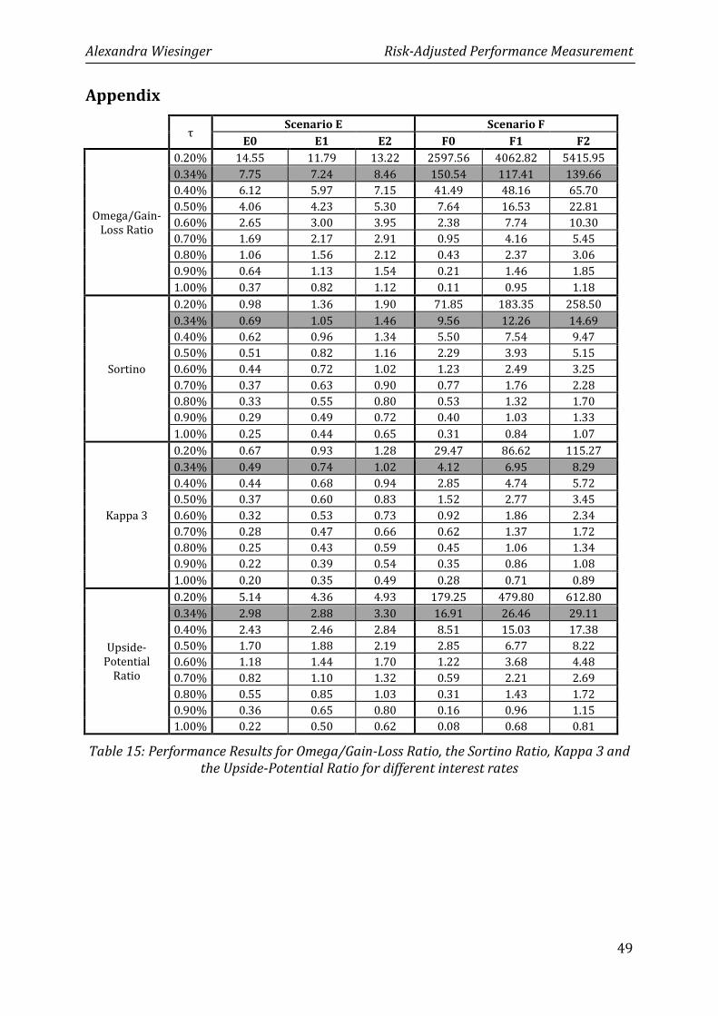
Alexandra Wiesinger Risk-Adjusted Performance Measurement
49
Appendix
τ Scenario E Scenario F
E0 E1 E2 F0 F1 F2
Omega/Gain-
Loss Ratio
0.20% 14.55 11.79 13.22 2597.56 4062.82 5415.95
0.34% 7.75 7.24 8.46 150.54 117.41 139.66
0.40% 6.12 5.97 7.15 41.49 48.16 65.70
0.50% 4.06 4.23 5.30 7.64 16.53 22.81
0.60% 2.65 3.00 3.95 2.38 7.74 10.30
0.70% 1.69 2.17 2.91 0.95 4.16 5.45
0.80% 1.06 1.56 2.12 0.43 2.37 3.06
0.90% 0.64 1.13 1.54 0.21 1.46 1.85
1.00% 0.37 0.82 1.12 0.11 0.95 1.18
Sortino
0.20% 0.98 1.36 1.90 71.85 183.35 258.50
0.34% 0.69 1.05 1.46 9.56 12.26 14.69
0.40% 0.62 0.96 1.34 5.50 7.54 9.47
0.50% 0.51 0.82 1.16 2.29 3.93 5.15
0.60% 0.44 0.72 1.02 1.23 2.49 3.25
0.70% 0.37 0.63 0.90 0.77 1.76 2.28
0.80% 0.33 0.55 0.80 0.53 1.32 1.70
0.90% 0.29 0.49 0.72 0.40 1.03 1.33
1.00% 0.25 0.44 0.65 0.31 0.84 1.07
Kappa 3
0.20% 0.67 0.93 1.28 29.47 86.62 115.27
0.34% 0.49 0.74 1.02 4.12 6.95 8.29
0.40% 0.44 0.68 0.94 2.85 4.74 5.72
0.50% 0.37 0.60 0.83 1.52 2.77 3.45
0.60% 0.32 0.53 0.73 0.92 1.86 2.34
0.70% 0.28 0.47 0.66 0.62 1.37 1.72
0.80% 0.25 0.43 0.59 0.45 1.06 1.34
0.90% 0.22 0.39 0.54 0.35 0.86 1.08
1.00% 0.20 0.35 0.49 0.28 0.71 0.89
Upside-
Potential
Ratio
0.20% 5.14 4.36 4.93 179.25 479.80 612.80
0.34% 2.98 2.88 3.30 16.91 26.46 29.11
0.40% 2.43 2.46 2.84 8.51 15.03 17.38
0.50% 1.70 1.88 2.19 2.85 6.77 8.22
0.60% 1.18 1.44 1.70 1.22 3.68 4.48
0.70% 0.82 1.10 1.32 0.59 2.21 2.69
0.80% 0.55 0.85 1.03 0.31 1.43 1.72
0.90% 0.36 0.65 0.80 0.16 0.96 1.15
1.00% 0.22 0.50 0.62 0.08 0.68 0.81
Table 15: Performance Results for Omega/Gain-Loss Ratio, the Sortino Ratio, Kappa 3 and the Upside-Potential Ratio for different interest rates
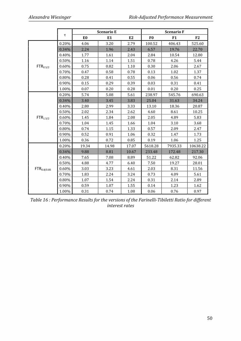
Alexandra Wiesinger Risk-Adjusted Performance Measurement
50
τ Scenario E Scenario F
E0 E1 E2 F0 F1 F2
FTR0.5/2
0.20% 4.06 3.20 2.79 100.52 406.43 525.60
0.34% 2.24 1.96 2.43 6.57 19.76 22.70
0.40% 1.77 1.61 2.04 2.84 10.54 12.80
0.50% 1.16 1.14 1.51 0.78 4.26 5.44
0.60% 0.75 0.82 1.10 0.30 2.06 2.67
0.70% 0.47 0.58 0.78 0.13 1.02 1.37
0.80% 0.28 0.41 0.55 0.06 0.56 0.74
0.90% 0.15 0.29 0.39 0.03 0.31 0.41
1.00% 0.07 0.20 0.28 0.01 0.20 0.25
FTR1.5/2
0.20% 5.74 5.08 5.61 238.97 545.76 690.63
0.34% 3.40 3.45 3.83 25.04 31.63 34.24
0.40% 2.80 2.99 3.33 13.10 18.36 20.87
0.50% 2.02 2.34 2.62 4.60 8.61 10.25
0.60% 1.45 1.84 2.08 2.05 4.89 5.83
0.70% 1.04 1.45 1.66 1.04 3.10 3.68
0.80% 0.74 1.15 1.33 0.57 2.09 2.47
0.90% 0.52 0.91 1.06 0.32 1.47 1.73
1.00% 0.36 0.72 0.85 0.19 1.06 1.25
FTR0.8/0.85
0.20% 19.34 14.98 17.07 5618.28 7935.33 10638.22
0.34% 9.88 8.81 10.67 233.48 172.48 217.30
0.40% 7.65 7.08 8.89 51.22 62.82 92.06
0.50% 4.88 4.77 6.40 7.50 19.27 28.01
0.60% 3.03 3.23 4.61 2.03 8.31 11.56
0.70% 1.83 2.24 3.24 0.73 4.09 5.61
0.80% 1.07 1.54 2.24 0.31 2.14 2.89
0.90% 0.59 1.07 1.55 0.14 1.23 1.62
1.00% 0.31 0.74 1.08 0.06 0.76 0.97
Table 16 : Performance Results for the versions of the Farinelli-Tibiletti Ratio for different interest rates
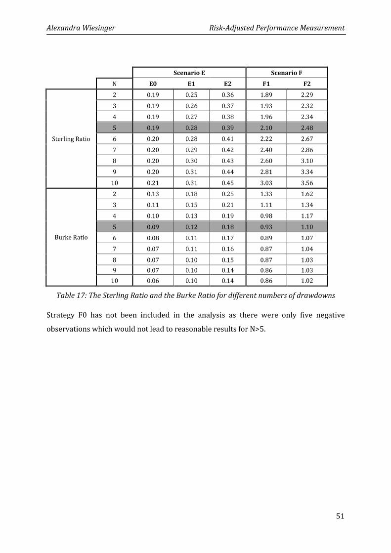
Alexandra Wiesinger Risk-Adjusted Performance Measurement
51
Scenario E Scenario F
N E0 E1 E2 F1 F2
Sterling Ratio
2 0.19 0.25 0.36 1.89 2.29
3 0.19 0.26 0.37 1.93 2.32
4 0.19 0.27 0.38 1.96 2.34
5 0.19 0.28 0.39 2.10 2.48
6 0.20 0.28 0.41 2.22 2.67
7 0.20 0.29 0.42 2.40 2.86
8 0.20 0.30 0.43 2.60 3.10
9 0.20 0.31 0.44 2.81 3.34
10 0.21 0.31 0.45 3.03 3.56
Burke Ratio
2 0.13 0.18 0.25 1.33 1.62
3 0.11 0.15 0.21 1.11 1.34
4 0.10 0.13 0.19 0.98 1.17
5 0.09 0.12 0.18 0.93 1.10
6 0.08 0.11 0.17 0.89 1.07
7 0.07 0.11 0.16 0.87 1.04
8 0.07 0.10 0.15 0.87 1.03
9 0.07 0.10 0.14 0.86 1.03
10 0.06 0.10 0.14 0.86 1.02
Table 17: The Sterling Ratio and the Burke Ratio for different numbers of drawdowns
Strategy F0 has not been included in the analysis as there were only five negative
observations which would not lead to reasonable results for N>5.

Alexandra Wiesinger Risk-Adjusted Performance Measurement
52
Eigenständigkeitserklärung
Ich erkläre hiermit,
− dass ich die vorliegende Arbeit ohne fremde Hilfe und ohne Verwendung anderer als
der angegebenen Hilfsmittel verfasst habe,
− dass ich sämtliche verwendeten Quellen erwähnt und gemäss gängigen
wissenschaftlichen Zitierregeln nach bestem Wissen und Gewissen korrekt zitiert habe.
St. Gallen, 21.Mai 2010 Alexandra Wiesinger


![[ba] Validity date from [BA] COUNTRY [ba] Viet Nam 00068 ... · PDF file[ba] Name [ba] City [ba] Regions [ba] Activities [ba] Remark [ba] Date of request ... DL 115 Nha Trang FISCO](https://img.pdfslide.us/doc/110x75/5a791ef27f8b9a9d218e108a/ba-validity-date-from-ba-country-ba-viet-nam-00068-ba-name-ba-city.jpg)


![[ba] Validity date from [BA] COUNTRY [ba] United States](https://img.pdfslide.us/doc/110x75/6191cacde75d406c8e1bf890/ba-validity-date-from-ba-country-ba-united-states-.jpg)