Wiener Deconvolution: Theoretical Basis

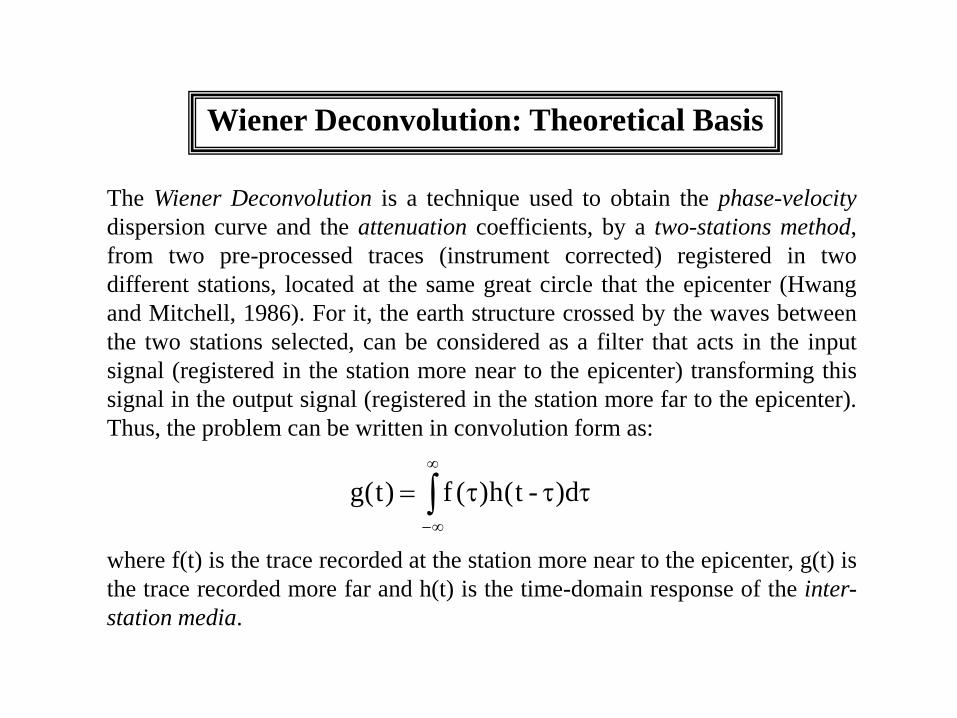
The Wiener Deconvolution is a technique used to obtain the phase-velocity dispersion curve and the attenuation coefficients, by a two-stations method, from two pre-processed traces (instrument corrected) registered in two different stations, located at the same great circle that the epicenter (Hwang and Mitchell, 1986). For it, the earth structure crossed by the waves between the two stations selected, can be considered as a filter that acts in the input signal (registered in the station more near to the epicenter) transforming this signal in the output signal (registered in the station more far to the epicenter). Thus, the problem can be written in convolution form as:

∫∞

∞−

τττ= d)-t(h)(f)t(g

where f(t) is the trace recorded at the station more near to the epicenter, g(t) is the trace recorded more far and h(t) is the time-domain response of the inter-station media.

Wiener Deconvolution: Theoretical Basis

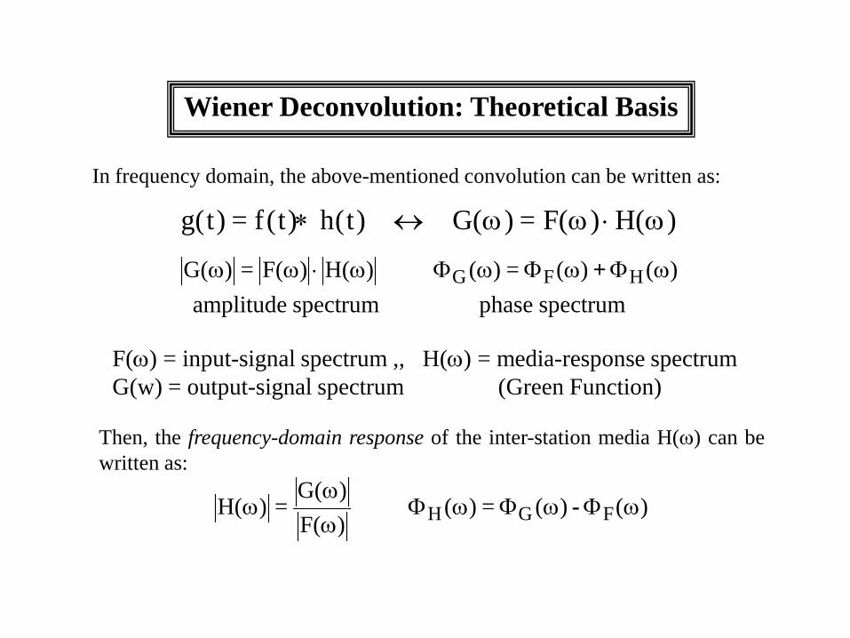
In frequency domain, the above-mentioned convolution can be written as:

g t f t t( ) = ( ) h( ) G( ) = F( ) H( )∗ ↔ ⋅ω ω ω

)( )(=)( )H()F(=)G( HFG ωΦωΦωΦω⋅ωω +

F(ω) = input-signal spectrum ,, H(ω) = media-response spectrum G(w) = output-signal spectrum (Green Function)

amplitude spectrum phase spectrum

Then, the frequency-domain response of the inter-station media H(ω) can be written as:

)( )(=)( )F()G(

=)H( FGH ωΦωΦωΦωω

ω -

Wiener Deconvolution: Theoretical Basis

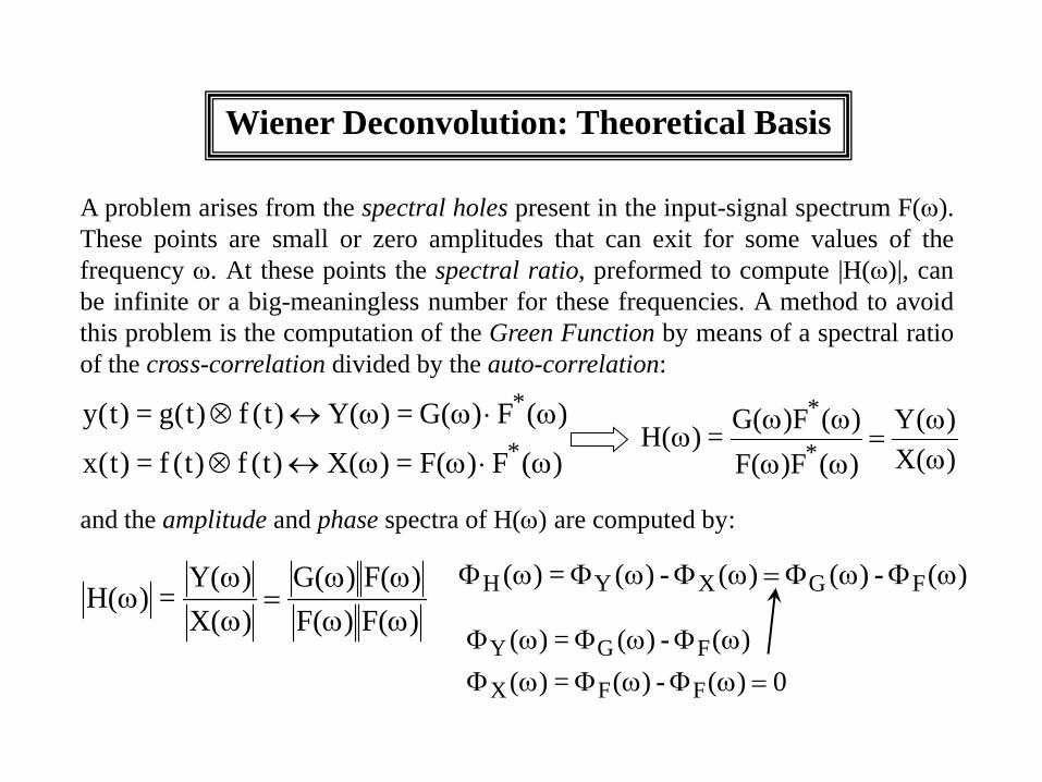
A problem arises from the spectral holes present in the input-signal spectrum F(ω). These points are small or zero amplitudes that can exit for some values of the frequency ω. At these points the spectral ratio, preformed to compute |H(ω)|, can be infinite or a big-meaningless number for these frequencies. A method to avoid this problem is the computation of the Green Function by means of a spectral ratio of the cross-correlation divided by the auto-correlation:

)(F)G(=)Y()t(f )t(g=)t(y * ω⋅ωω↔⊗

)(F)F(=)X()t(f )t(f=)t(x * ω⋅ωω↔⊗

)F()F()F()G(

)X()Y(

=)H(ωωωω

=ωω

ω

)(X)(Y

)()FF()()FG(=)H( *

*

ωω

=ωω

ωωω

and the amplitude and phase spectra of H(ω) are computed by:

0)( )(=)()( )(=)(

FFX

FGY=ωΦωΦωΦ

ωΦωΦωΦ - -

)( )()( )(=)( FGXYH ωΦωΦ=ωΦωΦωΦ - -

Wiener Deconvolution: Theoretical Basis

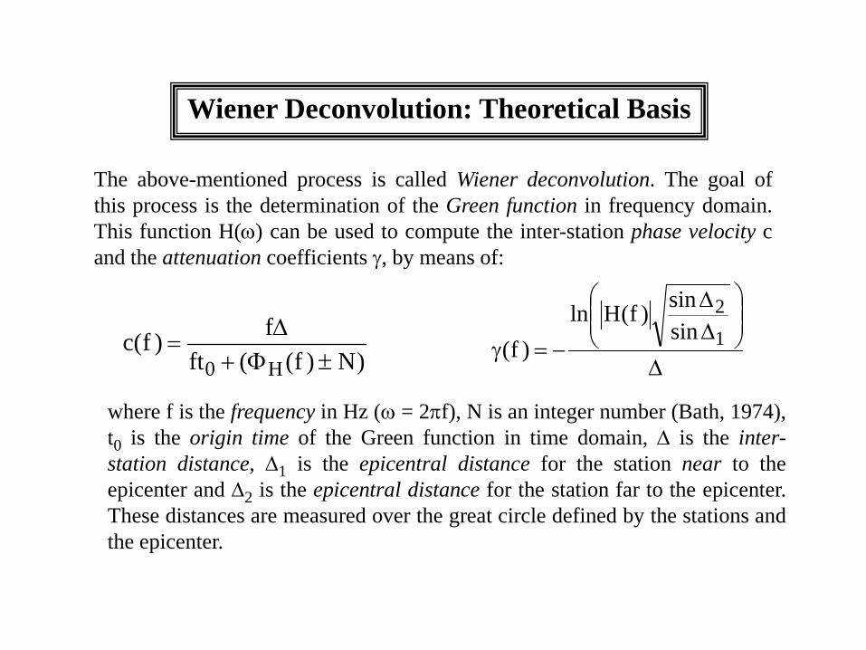
The above-mentioned process is called Wiener deconvolution. The goal of this process is the determination of the Green function in frequency domain. This function H(ω) can be used to compute the inter-station phase velocity c and the attenuation coefficients γ, by means of:

)N)f((ftf)f(cH0 ±Φ+∆

=∆

∆∆

−=γ 1

2sinsin)f(Hln

)f(

where f is the frequency in Hz (ω = 2πf), N is an integer number (Bath, 1974), t0 is the origin time of the Green function in time domain, ∆ is the inter-station distance, ∆1 is the epicentral distance for the station near to the epicenter and ∆2 is the epicentral distance for the station far to the epicenter. These distances are measured over the great circle defined by the stations and the epicenter.

Wiener Deconvolution: Theoretical Basis

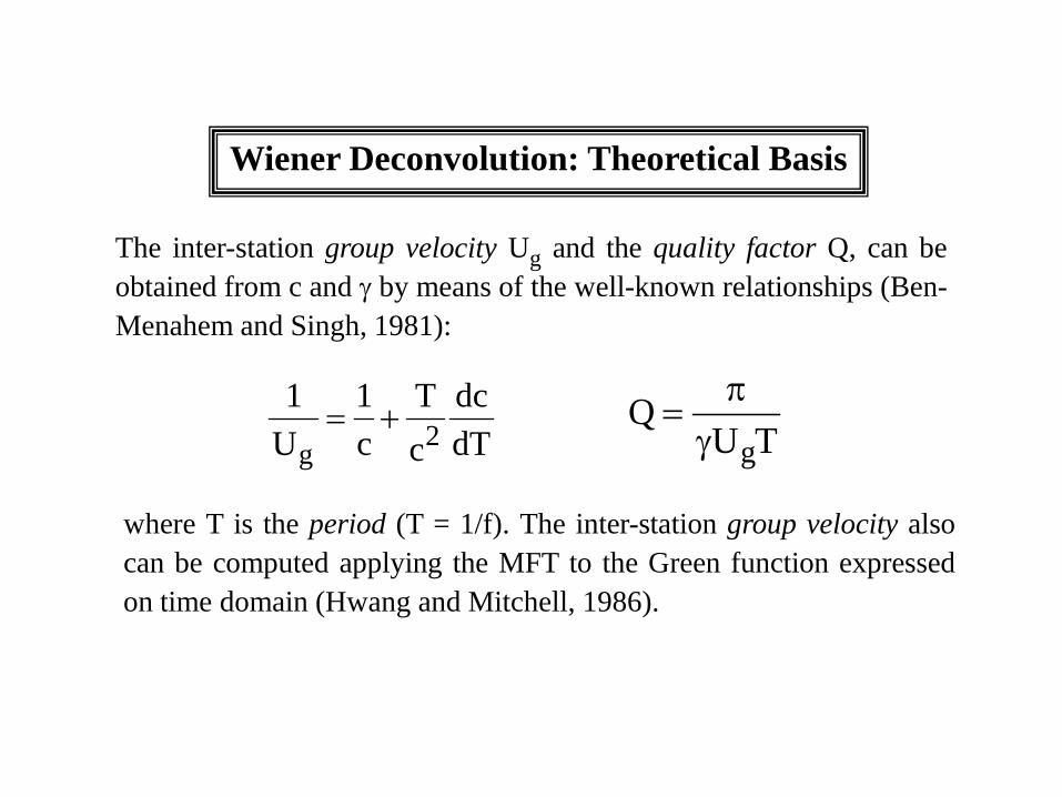
The inter-station group velocity Ug and the quality factor Q, can be obtained from c and γ by means of the well-known relationships (Ben-Menahem and Singh, 1981):

dTdc

cT

c1

U1

2g+=

TUQ

gγπ

=

where T is the period (T = 1/f). The inter-station group velocity also can be computed applying the MFT to the Green function expressed on time domain (Hwang and Mitchell, 1986).

Wiener Deconvolution: An Example

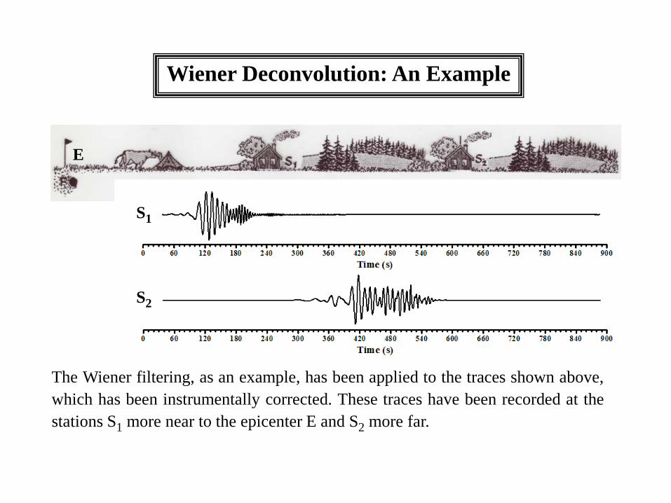
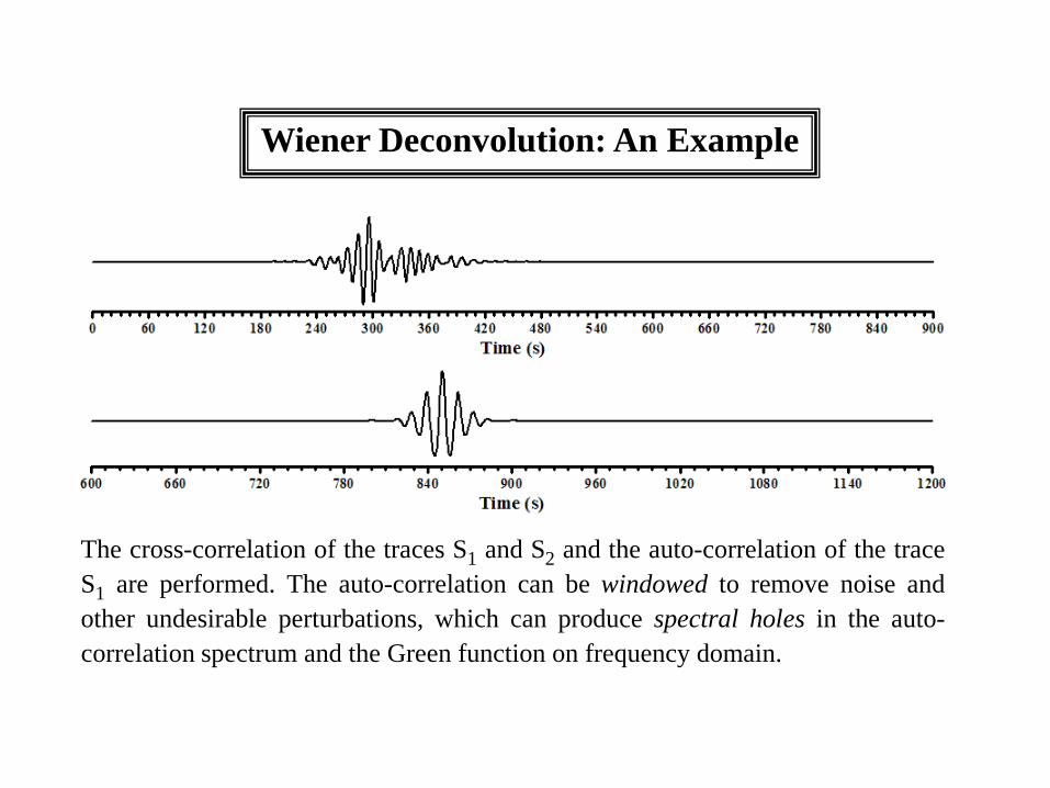
The Wiener filtering, as an example, has been applied to the traces shown above, which has been instrumentally corrected. These traces have been recorded at the stations S1 more near to the epicenter E and S2 more far.

S1

S2

E

Wiener Deconvolution: An Example

The cross-correlation of the traces S1 and S2 and the auto-correlation of the trace S1 are performed. The auto-correlation can be windowed to remove noise and other undesirable perturbations, which can produce spectral holes in the auto-correlation spectrum and the Green function on frequency domain.

Wiener Deconvolution: An Example

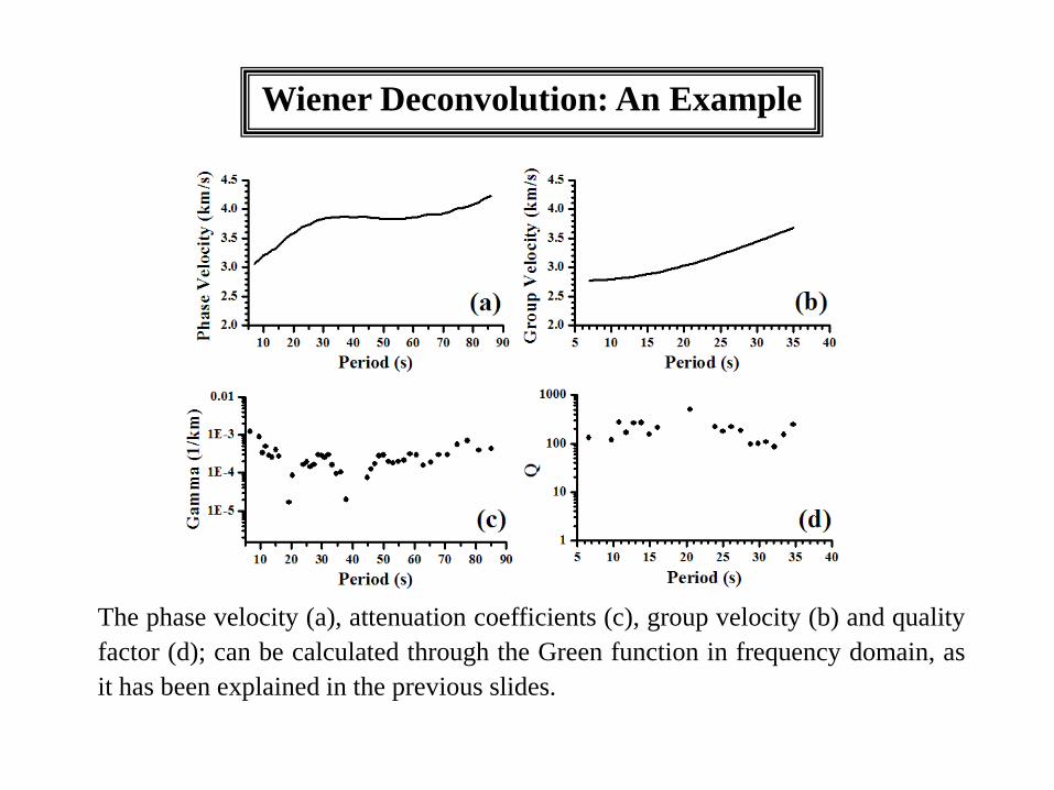
The phase velocity (a), attenuation coefficients (c), group velocity (b) and quality factor (d); can be calculated through the Green function in frequency domain, as it has been explained in the previous slides.

Wiener Deconvolution: References

Bath M. (1974). Spectral Analysis in Geophysics. Elsevier, Amsterdam.

Ben-Menahem A. and Singh S. J. (1981). Seismic Waves and Sources. Springer-Verlag, Berlin.

Hwang H. J. and Mitchell B. J. (1986). Interstation surface wave analysis by frequency-domain Wiener deconvolution and modal isolation. Bull. of the Seism. Soc. of America, 76, 847-864.

Wiener Deconvolution: Web Page

http://airy.ual.es/www/Wiener.htm

Approximation Theory

Given a Hilbert space H with an inner product ( , ) we de�ne

d('1; '2) = jj'1 � '2jj =p('1 � '2; '1 � '2)

Given a subspace S � H with a basis ( 1; 2; ; :::; n)

Any b' 2 S can be written as b' = nPi=1

�i i.

Problem: Given ' 2 H �nd b' 2 S so that jj'� b'jj is a minimumSolution: Choose ' so that

('� b'; v) = 0 for every v 2 S

1

Wiener Filter

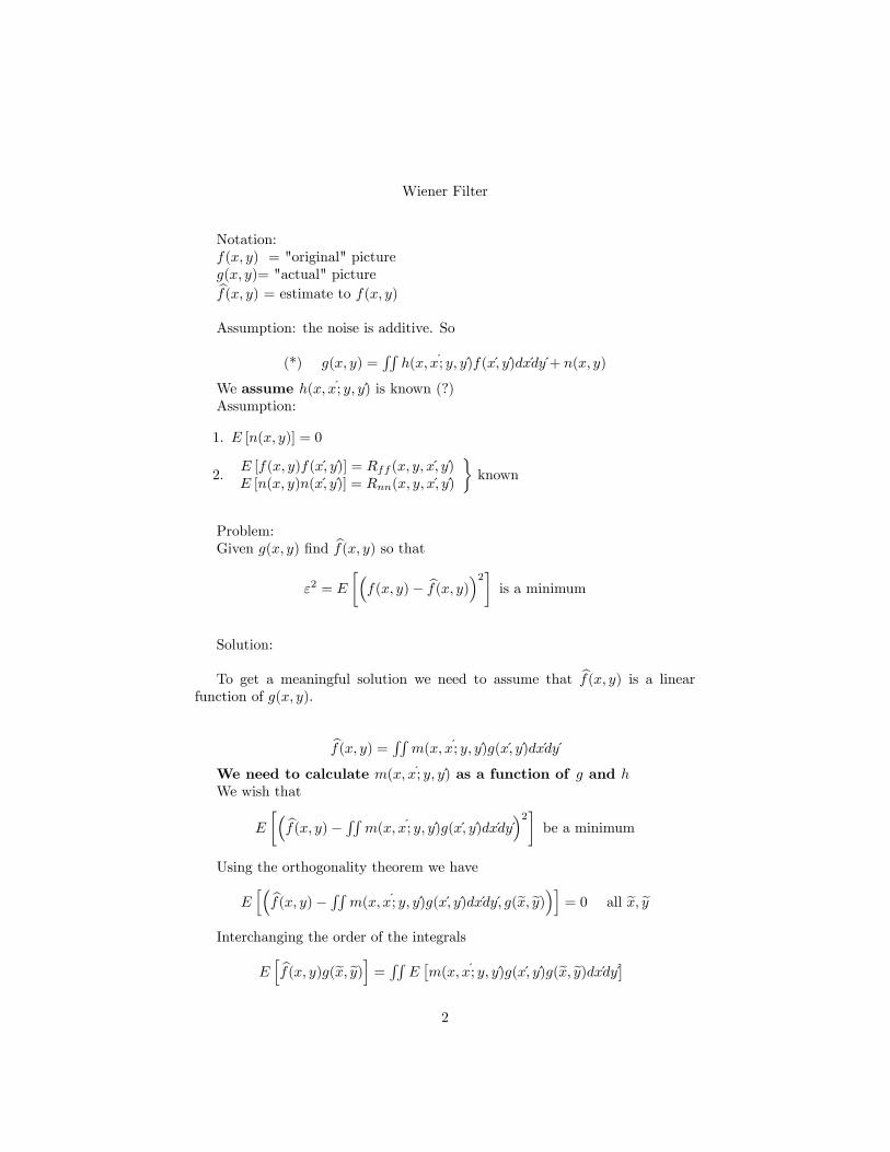
Notation:f(x; y) = "original" pictureg(x; y)= "actual" picturebf(x; y) = estimate to f(x; y)Assumption: the noise is additive. So

(*) g(x; y) =RR

h(x; x�; y; y�)f(x�; y�)dx�dy�+ n(x; y)

We assume h(x; x�; y; y�) is known (?)Assumption:

1. E [n(x; y)] = 0

2.E [f(x; y)f(x�; y�)] = Rff (x; y; x�; y�)E [n(x; y)n(x�; y�)] = Rnn(x; y; x�; y�)

�known

Problem:Given g(x; y) �nd bf(x; y) so that

"2 = E

��f(x; y)� bf(x; y)�2� is a minimum

Solution:

To get a meaningful solution we need to assume that bf(x; y) is a linearfunction of g(x; y).

bf(x; y) = RR m(x; x�; y; y�)g(x�; y�)dx�dy�We need to calculate m(x; x�; y; y�) as a function of g and hWe wish that

E

�� bf(x; y)� RR m(x; x�; y; y�)g(x�; y�)dx�dy��2� be a minimumUsing the orthogonality theorem we have

Eh� bf(x; y)� RR m(x; x�; y; y�)g(x�; y�)dx�dy�; g(ex; ey)�i = 0 all ex; ey

Interchanging the order of the integrals

Eh bf(x; y)g(ex; ey)i = RR E �m(x; x�; y; y�)g(x�; y�)g(ex; ey)dx�dy��

2

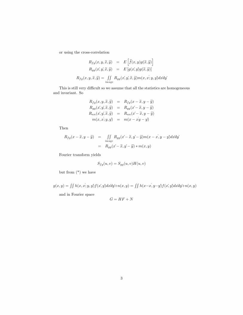
or using the cross-correlation

Rfg(x; y; ex; ey) = Eh bf(x; y)g(ex; ey)i

Rgg(x�; y�; ex; ey) = E [g(x�; y�)g(ex; ey)]Rfg(x; y; ex; ey) = RR

imageRgg(x�; y�; ex; ey)m(x; x�; y; y�)dx�dy�

This is still very di¢ cult so we assume that all the statistics are homogeneousand invariant. So

Rfg(x; y; ex; ey) = Rfg(x� ex; y � ey)Rgg(x�; y�; ex; ey) = Rgg(x�� ex; y � ey)Rnn(x�; y�; ex; ey) = Rnn(x�� ex; y � ey)m(x; x�; y; y�) = m(x� x�y � y�)

Then

Rfg(x� ex; y � ey) =RRimage

Rgg(x�� ex; y�� ey)m(x� x�; y � y�)dx�dy�= Rgg(x�� ex; y�� ey) �m(x; y)

Fourier transform yields

Sfg(u; v) = Sgg(u; v)H(u; v)

but from (*) we have

g(x; y) =RR

h(x; x�; y; y�)f(x�; y�)dx�dy�+n(x; y) =RR

h(x�x�; y�y�)f(x�; y�)dx�dy�+n(x; y)

and in Fourier spaceG = HF +N

3

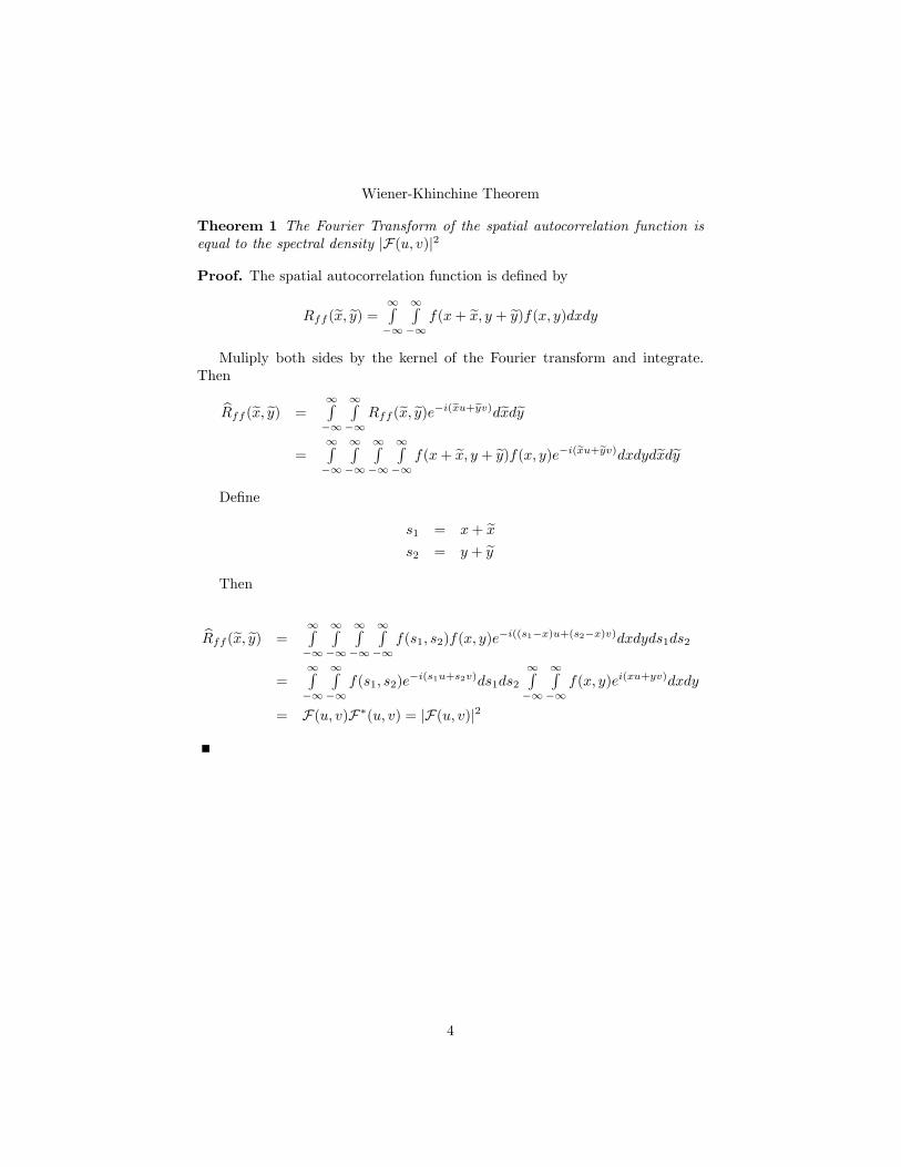
Wiener-Khinchine Theorem

Theorem 1 The Fourier Transform of the spatial autocorrelation function isequal to the spectral density jF(u; v)j2

Proof. The spatial autocorrelation function is de�ned by

Rff (ex; ey) = 1R�1

1R�1

f(x+ ex; y + ey)f(x; y)dxdyMuliply both sides by the kernel of the Fourier transform and integrate.

Then

bRff (ex; ey) =1R�1

1R�1

Rff (ex; ey)e�i(exu+eyv)dexdey=

1R�1

1R�1

1R�1

1R�1

f(x+ ex; y + ey)f(x; y)e�i(exu+eyv)dxdydexdeyDe�ne

s1 = x+ exs2 = y + ey

Then

bRff (ex; ey) =1R�1

1R�1

1R�1

1R�1

f(s1; s2)f(x; y)e�i((s1�x)u+(s2�x)v)dxdyds1ds2

=1R�1

1R�1

f(s1; s2)e�i(s1u+s2v)ds1ds2

1R�1

1R�1

f(x; y)ei(xu+yv)dxdy

= F(u; v)F�(u; v) = jF(u; v)j2

4

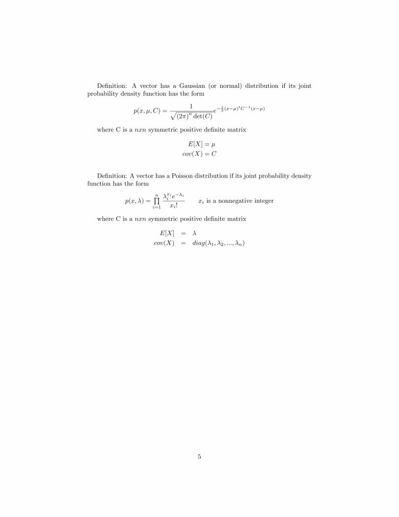
De�nition: A vector has a Gaussian (or normal) distribution if its jointprobability density function has the form

p(x; �; C) =1p

(2�)ndet(C)

e�12 (x��)

tC�1(x��)

where C is a nxn symmetric positive de�nite matrix

E[X] = �

cov(X) = C

De�nition: A vector has a Poisson distribution if its joint probability densityfunction has the form

p(x; �) =nQi=1

�xii e��i

xi!xi is a nonnegative integer

where C is a nxn symmetric positive de�nite matrix

E[X] = �

cov(X) = diag(�1; �2; :::; �n)

5

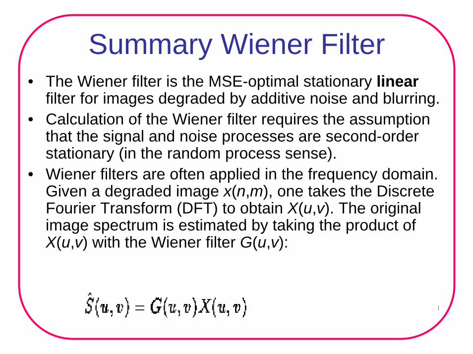
Summary Wiener Filter• The Wiener filter is the MSE-optimal stationary linear

filter for images degraded by additive noise and blurring. • Calculation of the Wiener filter requires the assumption

that the signal and noise processes are second-order stationary (in the random process sense).

• Wiener filters are often applied in the frequency domain. Given a degraded image x(n,m), one takes the Discrete Fourier Transform (DFT) to obtain X(u,v). The original image spectrum is estimated by taking the product of X(u,v) with the Wiener filter G(u,v):

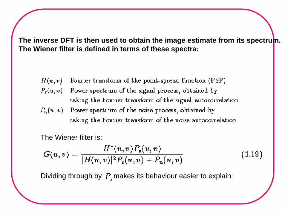
The inverse DFT is then used to obtain the image estimate from its spectrum. The Wiener filter is defined in terms of these spectra:

The Wiener filter is:

Dividing through by makes its behaviour easier to explain:

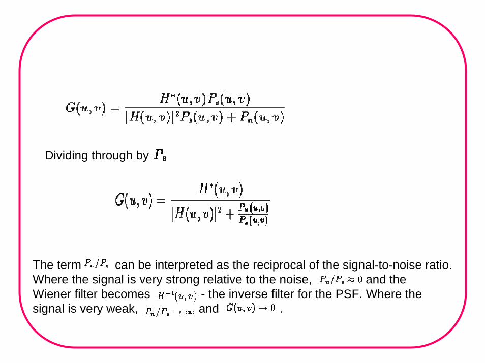
Dividing through by

The term can be interpreted as the reciprocal of the signal-to-noise ratio. Where the signal is very strong relative to the noise, and the Wiener filter becomes - the inverse filter for the PSF. Where the signal is very weak, and .

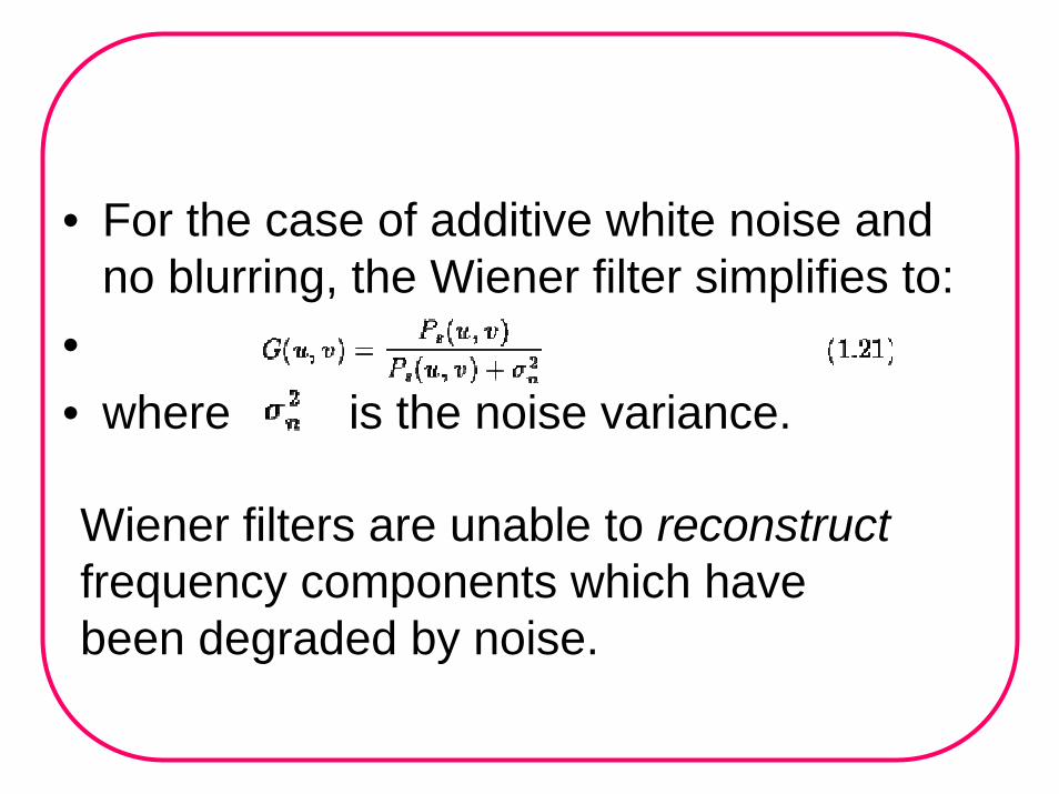
• For the case of additive white noise and no blurring, the Wiener filter simplifies to:

•• where is the noise variance.

Wiener filters are unable to reconstructfrequency components which have been degraded by noise.

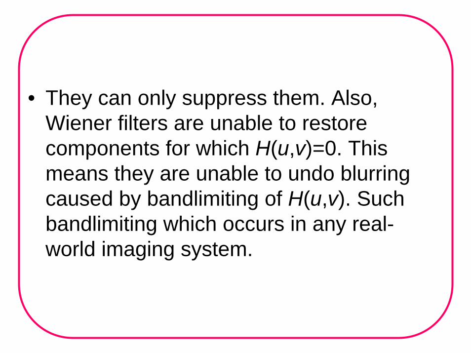
• They can only suppress them. Also, Wiener filters are unable to restore components for which H(u,v)=0. This means they are unable to undo blurring caused by bandlimiting of H(u,v). Such bandlimiting which occurs in any real-world imaging system.

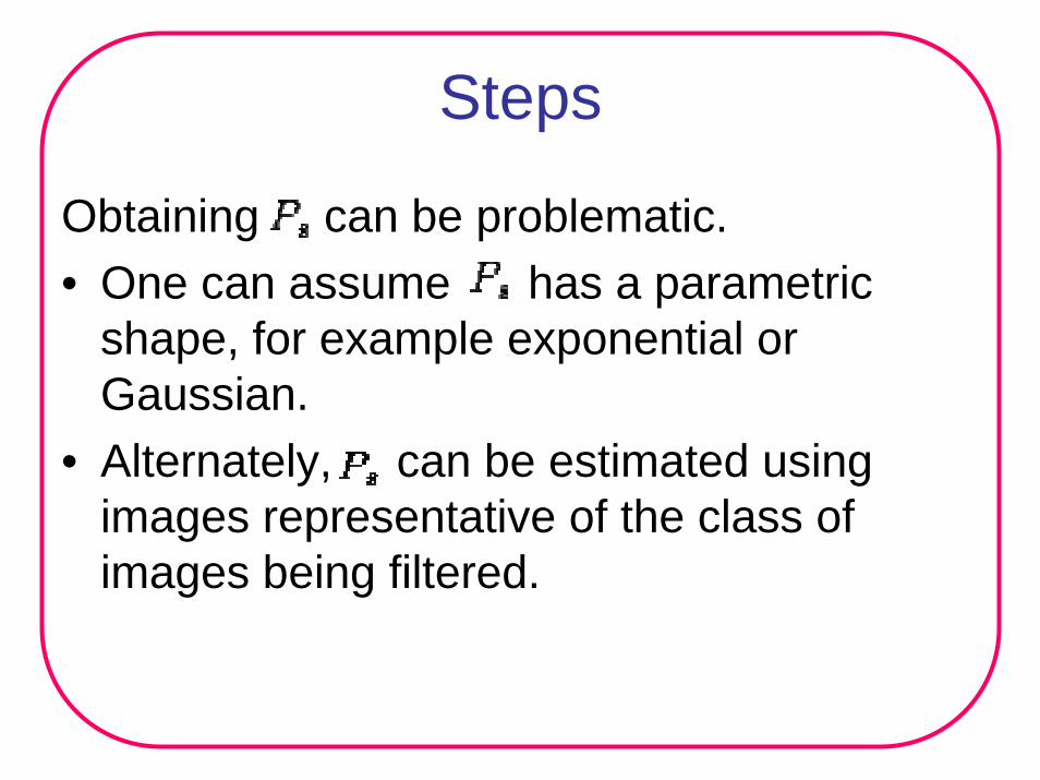
Steps

Obtaining can be problematic. • One can assume has a parametric

shape, for example exponential or Gaussian.

• Alternately, can be estimated using images representative of the class of images being filtered.

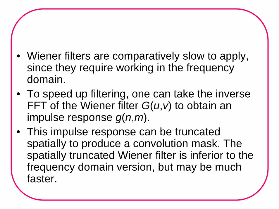
• Wiener filters are comparatively slow to apply, since they require working in the frequency domain.

• To speed up filtering, one can take the inverse FFT of the Wiener filter G(u,v) to obtain an impulse response g(n,m).

• This impulse response can be truncated spatially to produce a convolution mask. The spatially truncated Wiener filter is inferior to the frequency domain version, but may be much faster.

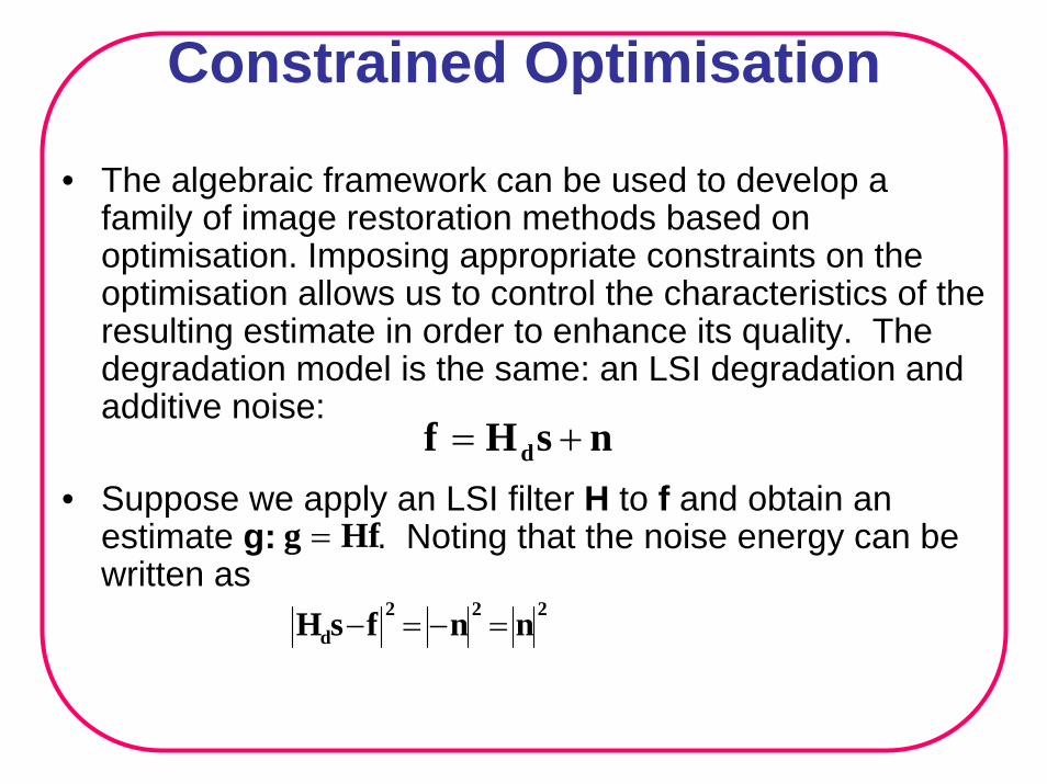
Constrained Optimisation

• The algebraic framework can be used to develop a family of image restoration methods based on optimisation. Imposing appropriate constraints on the optimisation allows us to control the characteristics of the resulting estimate in order to enhance its quality. The degradation model is the same: an LSI degradation and additive noise:

• Suppose we apply an LSI filter H to f and obtain an estimate g: . Noting that the noise energy can be written as

nsHf d +=

Hfg =

222d nnfsH =−=−

Filter Design Under Noise Constraints

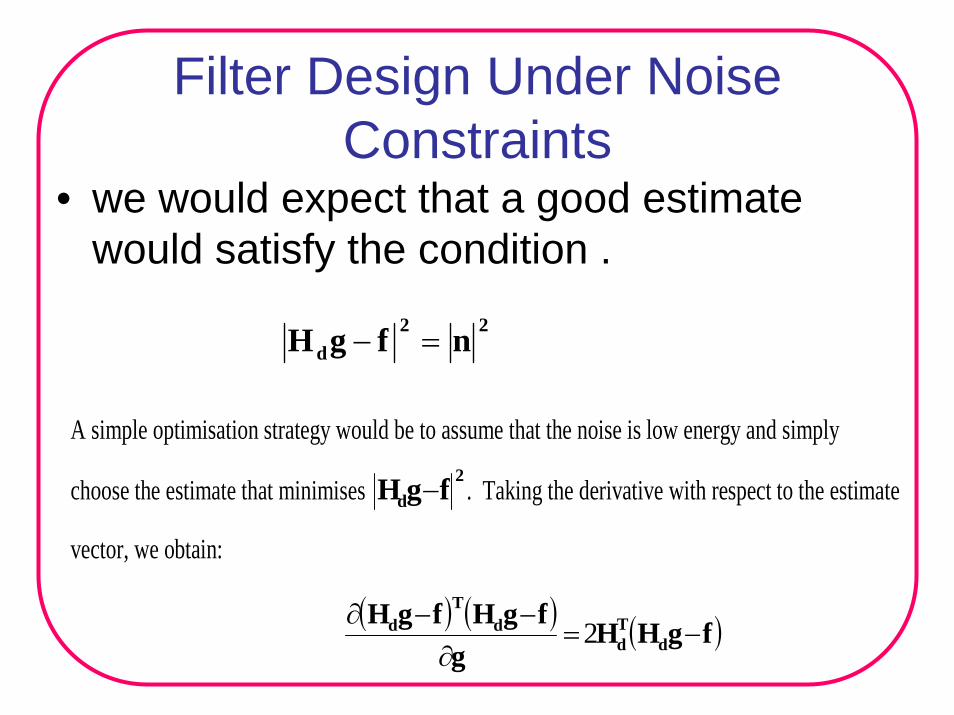
• we would expect that a good estimate would satisfy the condition .

22d nfgH =−

A simple optimisation strategy would be to assume that the noise is low energy and simply

choose the estimate that minimises 2

d fgH − . Taking the derivative with respect to the estimate

vector, we obtain:

( ) ( ) ( )fgHHg

fgHfgHd

Td

dT

d −=∂

−−∂2

Minimum Noise Assumption

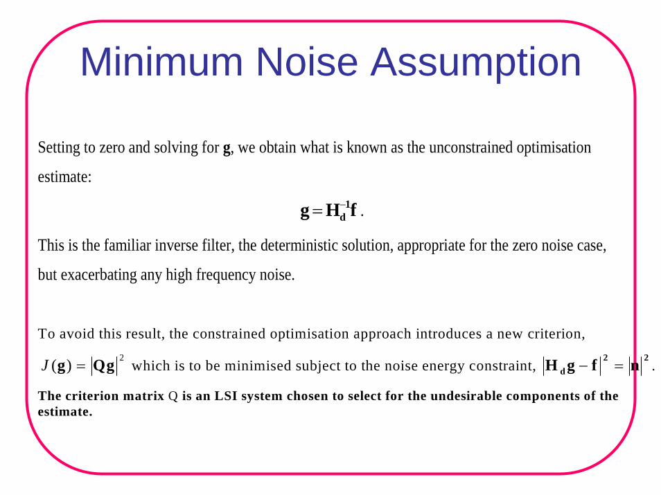
Setting to zero and solving for g, we obtain what is known as the unconstrained optimisation

estimate:

fHg 1d−= .

This is the familiar inverse filter, the deterministic solution, appropriate for the zero noise case,

but exacerbating any high frequency noise.

To avoid this result, the constrained optimisation approach introduces a new criterion, 2)( Qgg =J which is to be minimised subject to the noise energy constraint,

22d nfgH =− .

The criterion matrix Q is an LSI system chosen to select for the undesirable components of the estimate.

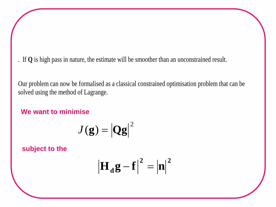
. If Q is high pass in nature, the estimate will be smoother than an unconstrained result.

Our problem can now be formalised as a classical constrained optimisation problem that can be solved using the method of Lagrange.

We want to minimise

2)( Qgg =Jsubject to the

22d nfgH =−

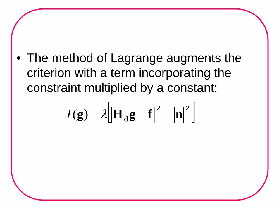
• The method of Lagrange augments the criterion with a term incorporating the constraint multiplied by a constant:

[ ]22d nfgHg −−+ λ)(J

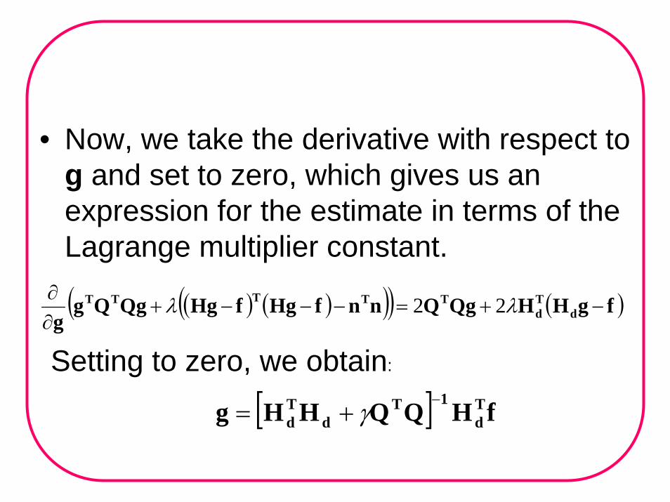
• Now, we take the derivative with respect to g and set to zero, which gives us an expression for the estimate in terms of the Lagrange multiplier constant.

( ) ( )( )( ) ( )fgHHQgQnnfHgfHgQgQgg d

Td

TTTTT −+=−−−+∂∂ λλ 22

Setting to zero, we obtain:

[ ] fHQQHHg Td

1Td

Td

−+= γ

• In principle, we impose the constraint in order to find the multiplier and thus obtain the estimate that satisfies the constraint.

• Unfortunately, there is no closed form expression for .

• While it is possible to employ an iterative technique, adjusting at each step to formally meet the constraint as closely as desired, in practice, is typically adjusted empirically along with the criterion matrix Q.

γλ 1=

λ

λ

λ

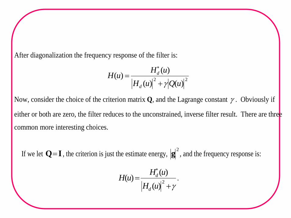
After diagonalization the frequency response of the filter is:

22 )()()(

)(uQuH

uHuH

d

d

γ+=

∗

Now, consider the choice of the criterion matrix Q, and the Lagrange constant γ . Obviously if

either or both are zero, the filter reduces to the unconstrained, inverse filter result. There are three

common more interesting choices.

If we let IQ= , the criterion is just the estimate energy, 2g , and the frequency response is:

γ+=

∗

2)()(

)(uH

uHuH

d

d .

• This simple filter is a pragmatic alternative to the Wiener filter when estimation of the signal and noise spectra are difficult.

• The constant is determined empirically to insure that at high frequencies, the degradation model has small frequency response,

)(1)( uHuH d∗≈

γrather than growing with frequency and amplifying high frequency noise like the inverse filter

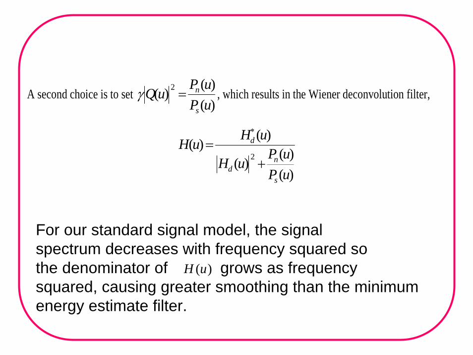
A second choice is to set )()(

)( 2

uPuP

uQs

n=γ , which results in the Wiener deconvolution filter,

)()(

)(

)()(

2

uPuP

uH

uHuH

s

nd

d

+=

∗

For our standard signal model, the signal spectrum decreases with frequency squared so the denominator of grows as frequency squared, causing greater smoothing than the minimum energy estimate filter.

)(uH

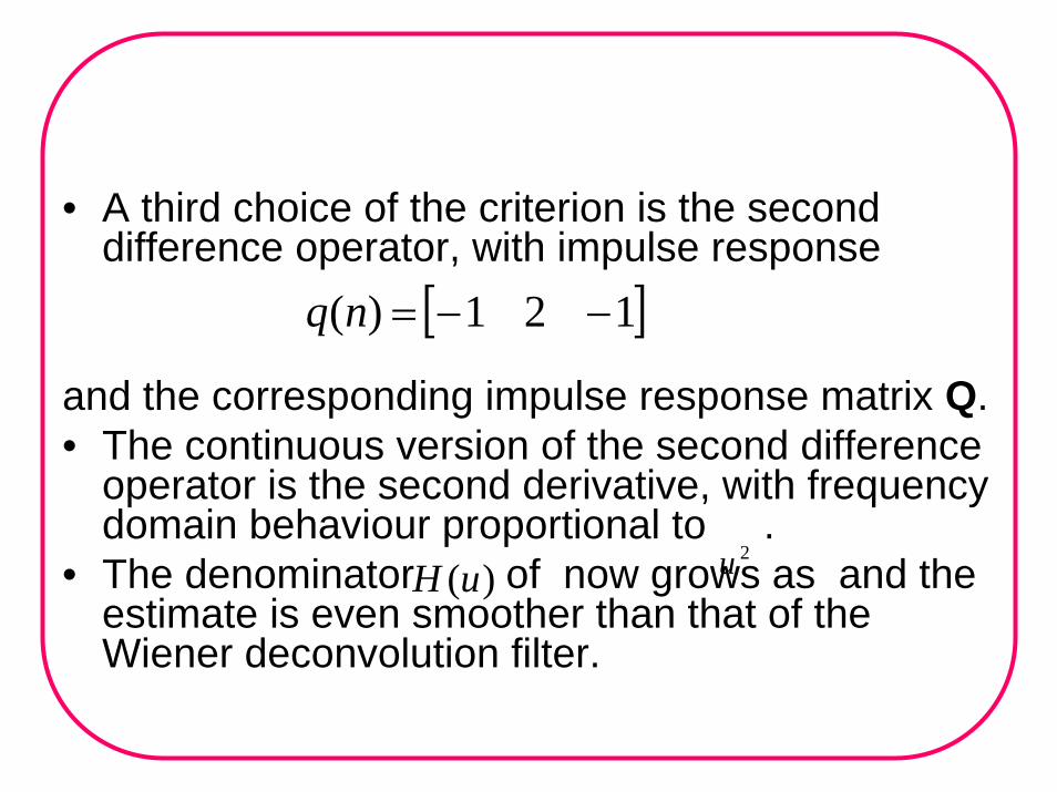
• A third choice of the criterion is the second difference operator, with impulse response

and the corresponding impulse response matrix Q. • The continuous version of the second difference

operator is the second derivative, with frequency domain behaviour proportional to .

• The denominator of now grows as and the estimate is even smoother than that of the Wiener deconvolution filter.

[ ]121)( −−=nq

2u)(uH

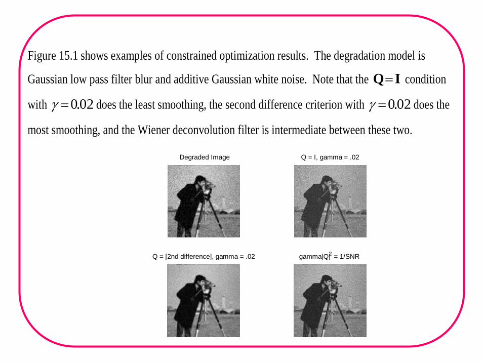
Figure 15.1 shows examples of constrained optimization results. The degradation model is

Gaussian low pass filter blur and additive Gaussian white noise. Note that the IQ= condition

with 02.0=γ does the least smoothing, the second difference criterion with 02.0=γ does the

most smoothing, and the Wiener deconvolution filter is intermediate between these two.

Degraded Image Q = I, gamma = .02

Q = [2nd difference], gamma = .02 gamma|Q|2 = 1/SNR

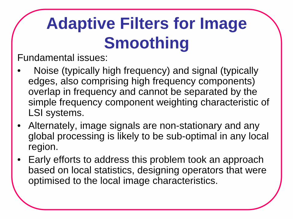
Adaptive Filters for Image Smoothing

Fundamental issues:• Noise (typically high frequency) and signal (typically

edges, also comprising high frequency components) overlap in frequency and cannot be separated by the simple frequency component weighting characteristic of LSI systems.

• Alternately, image signals are non-stationary and any global processing is likely to be sub-optimal in any local region.

• Early efforts to address this problem took an approach based on local statistics, designing operators that were optimised to the local image characteristics.

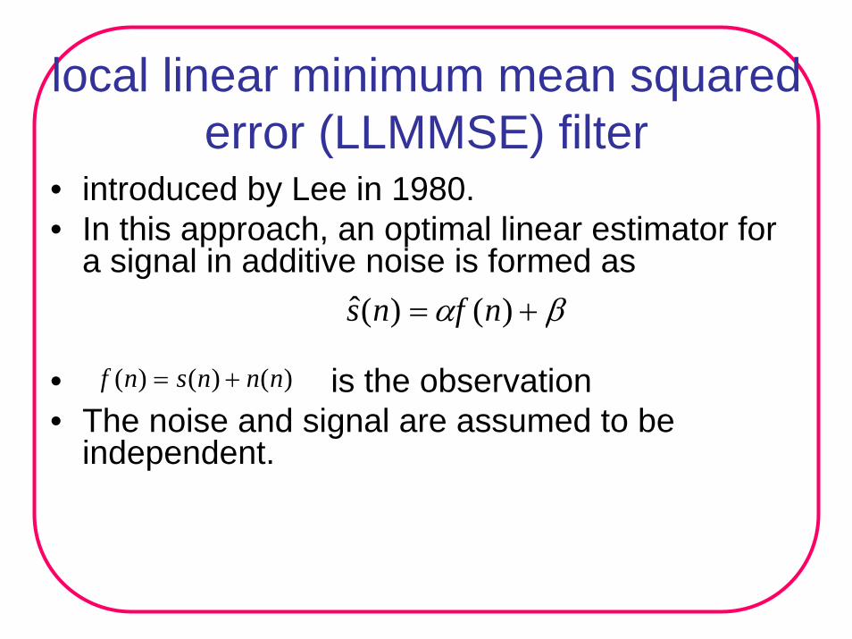
local linear minimum mean squared error (LLMMSE) filter

• introduced by Lee in 1980. • In this approach, an optimal linear estimator for

a signal in additive noise is formed as

• is the observation • The noise and signal are assumed to be

independent.

βα += )()(ˆ nfns

)()()( nnnsnf +=

α

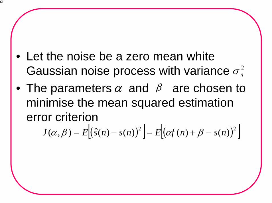
• Let the noise be a zero mean white Gaussian noise process with variance

• The parameters and are chosen to minimise the mean squared estimation error criterion

2nσ

α β

( )[ ] ( )[ ]22 )()()()(ˆ),( nsnfEnsnsEJ −+=−= βαβα

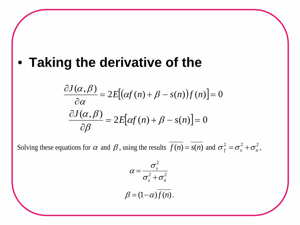
• Taking the derivative of the

( )[ ] 0)()()(2),(=−+=

∂∂ nfnsnfEJ βα

αβα

[ ] 0)()(2),(=−+=

∂∂ nsnfEJ βα

ββα

Solving these equations for α and β , using the results )()( nsnf = and 222nsf σσσ += ,

22

2

ns

s

σσσ

α+

=

)()1( nfαβ −= .

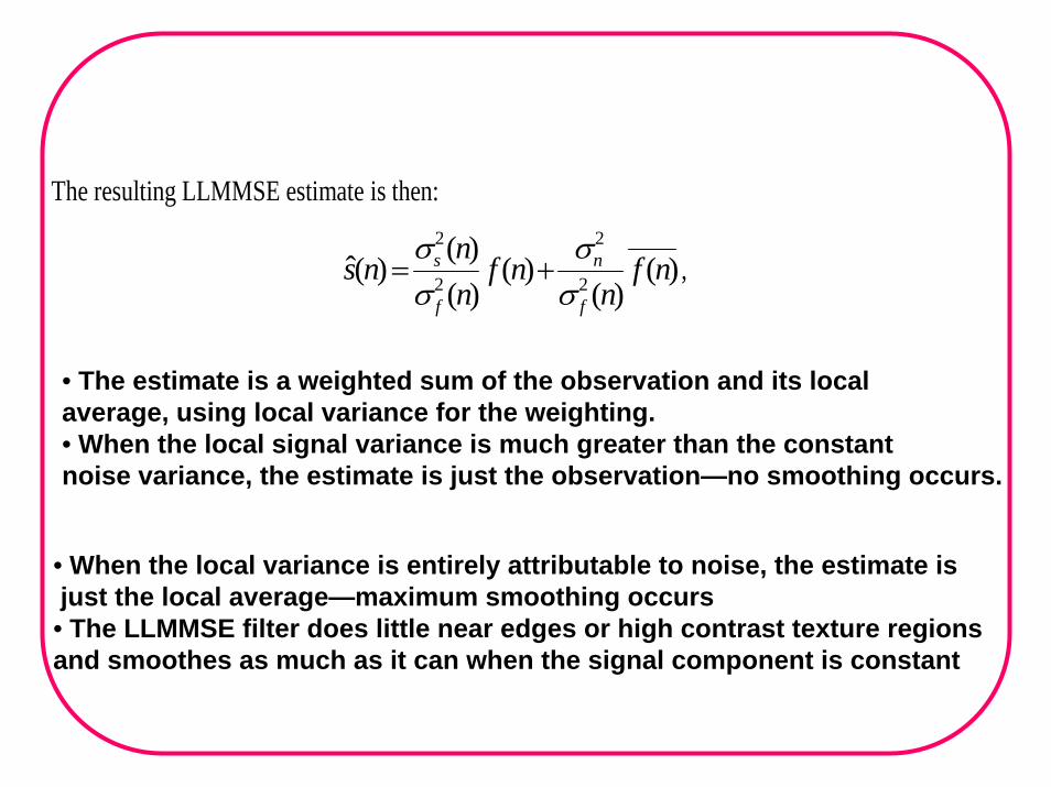
The resulting LLMMSE estimate is then:

)()(

)()()(

)(̂ 2

2

2

2

nfn

nfnn

nsf

n

f

s

σσ

σσ

+= ,

• The estimate is a weighted sum of the observation and its localaverage, using local variance for the weighting. • When the local signal variance is much greater than the constant noise variance, the estimate is just the observation—no smoothing occurs.

• When the local variance is entirely attributable to noise, the estimate isjust the local average—maximum smoothing occurs• The LLMMSE filter does little near edges or high contrast texture regions and smoothes as much as it can when the signal component is constant

• Note that we have to estimate the noise variance somehow, as we did with the conventional Wiener filter.

• The choice of window size over which to estimate the local mean and variance is important.

• It needs to be at least for reasonable variance estimates, but it should be small enough to insure local signal stationarity.

• Lee found that both 5x5 and 7x7 worked well.

55×

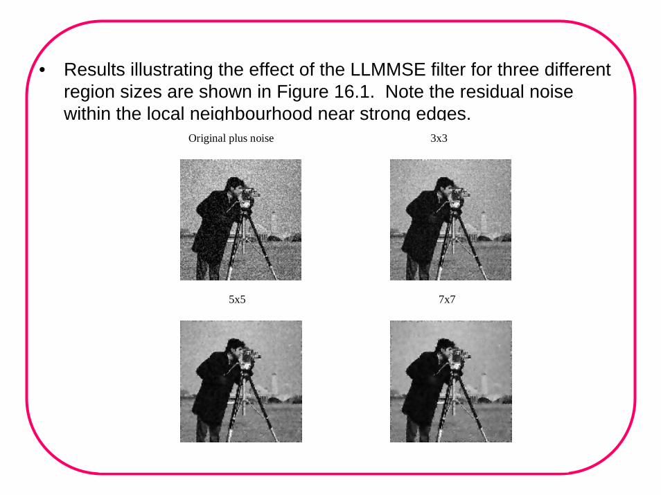
• Results illustrating the effect of the LLMMSE filter for three different region sizes are shown in Figure 16.1. Note the residual noise within the local neighbourhood near strong edges.

Original plus noise 3x3

5x5 7x7

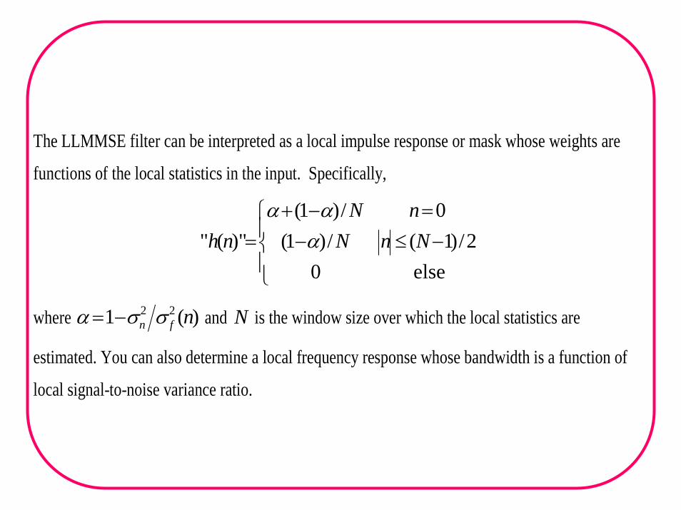
The LLMMSE filter can be interpreted as a local impulse response or mask whose weights are

functions of the local statistics in the input. Specifically,

⎪⎩

⎪⎨

⎧−≤−=−+

=else0

2/)1(/)1(0/)1(

)"(" NnNnN

nh ααα

where )(1 22 nfn σσα −= and N is the window size over which the local statistics are

estimated. You can also determine a local frequency response whose bandwidth is a function of

local signal-to-noise variance ratio.

Limitations of the LLMMSE filter are apparent.

• The need to restrict the window's size to achieve local stationarity restricts the amount of smoothing that can be achieved in constant signal regions.

• It may be desirable to allow the smoothing window to grow as large as the signal constant region allows.

• Some alternate noise suppression scheme to simple averaging should be employed, such as a local order-statistic filter (median filter and the like, which we will discuss further later).

• Alternately, it may be desirable to apply the LLMMSE filter iteratively, achieving repeated smoothing in constant signal regions. The window's square shape is also a limitation.

• Near an edge, the LLMMSE filter does no smoothing, allowing visible noise in close proximity to the edge.

• The window shape should also adapt, allowing the filter to smooth along but not across edges.

• The constant weights within the window, except for the centre point, limit the smoothing to the box filter, or simple local averaging variety.

• Perhaps some sort of locally variable weighting within the window would improve the performance near edges.

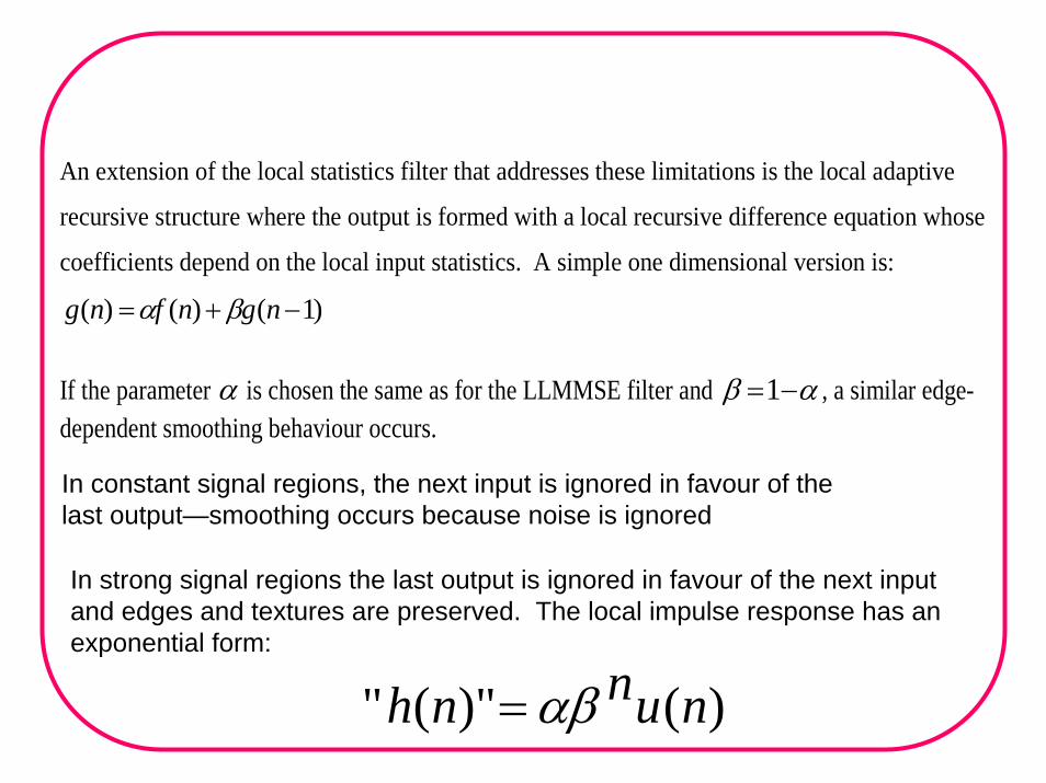
An extension of the local statistics filter that addresses these limitations is the local adaptive

recursive structure where the output is formed with a local recursive difference equation whose

coefficients depend on the local input statistics. A simple one dimensional version is:

)1()()( −+= ngnfng βα

If the parameter α is chosen the same as for the LLMMSE filter and αβ −=1 , a similar edge-dependent smoothing behaviour occurs.

In constant signal regions, the next input is ignored in favour of the last output—smoothing occurs because noise is ignored

In strong signal regions the last output is ignored in favour of the next input and edges and textures are preserved. The local impulse response has an exponential form:

)()"(" nunnh αβ=

• It is as if both the weights within the window and the window size are now dependent on the local signal-to-noise variance ratio (SNR).

• As the local SNR decreases, increases, the weights become more uniform and the impulse response extends over a larger interval, and more smoothing occurs.

β

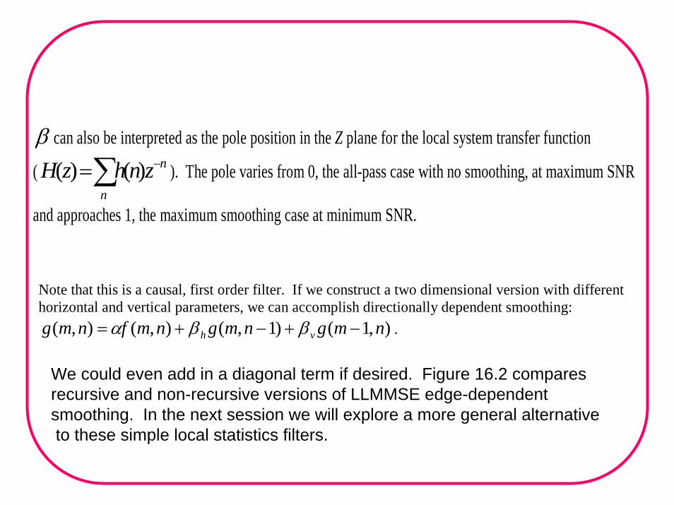
β can also be interpreted as the pole position in the Z plane for the local system transfer function

( ∑ −=n

nznhzH )()( ). The pole varies from 0, the all-pass case with no smoothing, at maximum SNR

and approaches 1, the maximum smoothing case at minimum SNR.

Note that this is a causal, first order filter. If we construct a two dimensional version with different horizontal and vertical parameters, we can accomplish directionally dependent smoothing:

),1()1,(),(),( nmgnmgnmfnmg vh −+−+= ββα .

We could even add in a diagonal term if desired. Figure 16.2 compares recursive and non-recursive versions of LLMMSE edge-dependent smoothing. In the next session we will explore a more general alternativeto these simple local statistics filters.

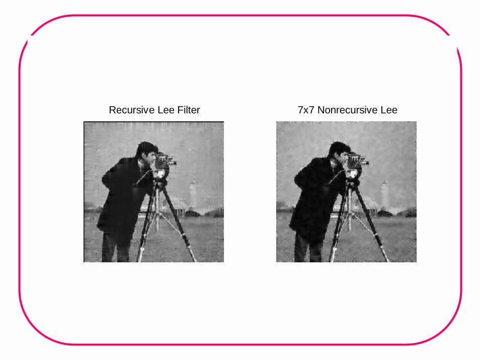
Recursive Lee Filter 7x7 Nonrecursive Lee