1 Washington University in St Louis, galiani@wustl.edu. 2 Universidad Torcuato Di Tella, eschargr@utdt.edu. This study has been prepared within the UNU-WIDER project on Land Inequality and Decentralized Governance in LDCs, directed by Pranab Bardhan and Dilip Mookherjee. UNU-WIDER acknowledges the financial contributions to the research programme by the governments of Denmark (Ministry of Foreign Affairs), Finland (Ministry for Foreign Affairs), Sweden (Swedish International Development Cooperation Agency—Sida) and the United Kingdom (Department for International Development).

Working Paper No. 2011/88

The Dynamics of Land Titling Regularization and Market Development Sebastian Galiani1 and Ernesto Schargrodsky2 December 2011

Abstract

We study the effects of titles on parcel valuation and urban land market development (real estate transfers, rentals, and mortgages), and the dynamics of deregularization by exploiting a natural experiment in the allocation of land titles to very poor families in a suburban area of Buenos Aires, Argentina. This natural experiment has been previously exploited to study effects of land titling on child health (Galiani and Schargrodsky 2004), on the formation of beliefs (Di Tella et al. 2007), and on investment, credit access, household structure, and educational achievement (Galiani and Schargrodsky 2010). Keywords: land titling, deregularization, titling premium JEL classification: O10, P14, Q15

The World Institute for Development Economics Research (WIDER) was established by the United Nations University (UNU) as its first research and training centre and started work in Helsinki, Finland in 1985. The Institute undertakes applied research and policy analysis on structural changes affecting the developing and transitional economies, provides a forum for the advocacy of policies leading to robust, equitable and environmentally sustainable growth, and promotes capacity strengthening and training in the field of economic and social policy making. Work is carried out by staff researchers and visiting scholars in Helsinki and through networks of collaborating scholars and institutions around the world. www.wider.unu.edu publications@wider.unu.edu

UNU World Institute for Development Economics Research (UNU-WIDER) Katajanokanlaituri 6 B, 00160 Helsinki, Finland Typescript prepared by Anne Ruohonen at UNU-WIDER The views expressed in this publication are those of the author(s). Publication does not imply endorsement by the Institute or the United Nations University, nor by the programme/project sponsors, of any of the views expressed.

Acknowledgements

We are grateful to Gestion Urbana, the NGO that performed the survey, Daniel Galizzi, Isabel Iñiguez, Bernardo Silberman, Claudio D’Alessandro, Pablo Gualchi (Land Undersecretary of the Province of Buenos Aires), and Juan Casazza for crucial cooperation, participants at the UNU-WIDER project meeting on Land Inequality, Conflict and Reform in LDCs, Hanoi, Vietnam, January 2011, and the Inter-American Development Bank, the Lincoln Institute of Land Policy and the Weidenbaum Center for financial support. Ramiro Galvez provided superb research assistance. Tables and figures appear at the end of the paper.

1

1. Introduction

The lack of well-defined land property rights may hamper the development of land markets. Selling, renting, and collateralizing land parcels might be impeded by the lack of titles. Some of these transactions can still be done without titles, but at a premium. This imposes considerable transaction costs on poor families, who are restricted from the possibility of exchanging houses at full value when their location, size or characteristics become inconvenient. Thus, the non-entitled may lose potential trade gains (Besley 1995). The first objective of this study is to estimate the titling transfer premium: the difference in real estate value paid for a house of similar characteristics between titled and untitled properties. The estimation of these premia might be complicated by differences in housing quality associated, themselves, to titling. The fragility of property rights is a crucial obstacle for economic development. Individuals underinvest if others can seize the fruits of their investments (Demsetz 1967; Alchian and Demsetz 1973; North and Thomas 1973; North 1981; De Long and Shleifer 1993; Besley 1995). Thus, inadequate property rights may affect the incentives to invest in housing quality. The estimation of titling premia needs to disentangle endogenous differences in housing quality. Thus, we aim to identify differences in housing value directly due to titling differences, not from differences in housing quality induced by titling differences.1 In addition to study whether untitled transactions sacrifice value, we also aim to investigate whether titling fosters the development of a rental, purchase and mortgage housing market. The lack of land titles may obstruct house rentals. The fear of expropriation by the renter might prevent usufructuary (i.e., legally untitled) owners from offering their houses for rent. The titling premium might make untitled sales less attractive. Receiving mortgage credit from formal financial institutions on untitled parcels is just not possible. We analyze the effect of titling on rentals, purchase and mortgage transactions. We also investigate what happens after land titling. In recent years, many governments throughout the developing world launched land-titling programmes as part of their poverty alleviation and urbanization policies. Typically, these programmes consist of titling public (or sometimes private) tracts of land to their current occupants. However, in most cases they are not accompanied by regulatory policies that alleviate the burden of titling registration of future ownership changes. Thus, as time goes by, and as the beneficiary titleholders pass away, divorce, or migrate, if these poor households cannot afford the costs of remaining formal, we will observe a slow process of deregularization leading to a new need for costly titling interventions.2

1 The estimation of titling premia could also be obscured by differences in access to credit. Titled houses in poor communities might be more in demand (and therefore reach higher prices) if their buyers qualify for mortgage credit (De Soto 2000). However, recent contributions show negligible effects of titling programmes on credit access (Feder et al. 1988; Place and Migot-Adholla 1998; Carter and Olinto 2003; Field and Torero 2003; Galiani and Schargrodsky 2010). 2 The story of Griselda, who lives in the neighbourhood under study, sadly illustrates the process and social costs of deregularization. The parcel where she lives was titled to her mother-in-law some years ago. After that, the mother-in-law passed away, but the son had no resources to go through the costly

2

Several authors have documented the effects of land property rights and titling programmes on different variables. A partial listing includes Jimenez (1984), Alston et al. (1996) and Lanjouw and Levy (2002) on real estate values; Besley (1995), Brasselle et al. (2002), Field (2005), and Do and Iyer (2008) on investment; Banerjee et al. (2002) and Libecap and Lueck (2008) on agricultural productivity; Field (2007) on labour supply; Vogl (2007) on child health; and Feder et al. (1988), Place and Migot-Adholla (1998), Carter and Olinto (2003), and Field and Torero (2003) on access to credit. Thus, in this paper, we study the effects of titles on parcel valuation and urban land market development (real estate transfers, rentals, and mortgages), and the dynamics of deregularization by exploiting a natural experiment in the allocation of land titles to very poor families in a suburban area of Buenos Aires, Argentina. This natural experiment has been previously exploited to study effects of land titling on child health (Galiani and Schargrodsky 2004), on the formation of beliefs (Di Tella et al. 2007), and on investment, credit access, household structure and educational achievement (Galiani and Schargrodsky 2010). These previous studies have not analyzed impacts on the variables considered in this new study; they could not have done it because the expropriation law that generated the natural experiment placed a restriction on land transfers that has only expired for all the titled parcels as of 2008, after the data were collected for those studies. The rest of the paper is organized as follows. In the next section we describe the natural experiment. Section 3 describes our data, and section 4 discusses the identification methods. Section 5 evaluates the titling premium and other empirical results. The deregularization process is documented in section 6, while section 7 concludes.

2. A natural experiment

The empirical evaluation of the effects of land titling poses a major methodological challenge. The allocation of property rights across families is typically not random but based on wealth, family characteristics, individual effort, previous investment levels, or other selective mechanisms. Thus, the individual characteristics that determine the likelihood of receiving land titles are probably correlated with the outcomes under study. Since some of these personal characteristics are unobservable, this correlation creates a selection problem that obstructs the proper evaluation of the effects of property right acquisition. In this project, we address this selection problem to study the effects of titles on land valuation by exploiting a natural experiment in the allocation of property rights. In 1981, about 1,800 families occupied a piece of wasteland in San Francisco Solano, County of Quilmes, in the Province of Buenos Aires. The occupants were groups of landless citizens organized through a Catholic chapel. As they wanted to avoid creating a shantytown, they partitioned the occupied land into small urban-shaped parcels. At the inheritance process. Later on, the couple separated due to his frequent violence against her. But they also lacked the resources to afford a legal divorce. Thus, they currently all live in the same parcel: she lives in a house in the front with two children, he lives in another room built in the back, and he still hits her. However, she cannot go to another place to live, nor evict him, and they have no way to legally split the parcel or its value as it still is under the name of his deceased mother.

3

beginning of the occupation the squatters believed that the land belonged to the state, but it was actually private property.3 The occupants resisted several attempts of eviction during the military government. After Argentina's return to democracy, the Congress of the Province of Buenos Aires passed Law Nº 10.239 in 1984 expropriating these lands from the former owners to allocate them to the squatters. According to the expropriation law, the government would pay a monetary compensation to the former owners and it would then allocate the land to the squatters. In order to qualify for receiving the titles, the squatters should have arrived to the parcels at least one year before the sanctioning of the law, should not possess any other property, and should use the parcel as their family home. Within each household, the titles would be awarded to both the household head identified at that time and to her/his spouse (if married or cohabitating). Importantly, the law also established that the squatters could not transfer the property of the parcels for the first ten years after titling. The process of expropriation resulted to be asynchronous and incomplete. The occupied area turned out to be composed of thirteen tracts of land belonging to different owners. In 1986, the government offered each owner a payment proportional to the official valuation of each tract of land, indexed by inflation. These official valuations, assessed by the tax authority to calculate property taxes, had been set before the land occupation. After the government made the compensation offers, the owner/s of each tract had to decide whether to surrender the land (accepting the expropriation compensation) or to start a legal dispute. Eight former owners accepted the compensation offered by the government. Five former owners, instead, did not accept the government offer and filed charges with the aim of obtaining a higher compensation. In 1989, the tracts of land of the former owners that accepted the government compensation were transferred to the squatters occupying them, together with formal land titles that secured the property of the parcels. The squatters that received titles in 1989 constitute the early-treated group in our study. The ten-year restriction on legal transactions expired for this group in 1999. The people who occupied parcels located on the tracts of land that belonged to the former owners that accepted the expropriation compensation, were ex-ante similar, and arrived at the same time, than the people who settled on the tracts of the former owners that did not surrender the land. There was simply no way for the occupants to know ex-ante, at the time of the occupation, which parcels of land had owners who would accept the compensation and which parcels had owners who would dispute it. In fact, at the time of the occupation the squatters believed that all the land was state-owned and they could not know that an expropriation law was going to be passed, nor what was going to be the future response of the owner of each specific parcel. A potential concern, however, is that the different former owners’ decisions could reflect differences in land quality. In turn, these differences could be correlated with squatters’ heterogeneity. For example, more powerful squatters could have settled in the best parcels. An advantage of our experiment is that the parcels of land in the treatment (titled) and control (untitled) groups are almost identical and basically next to each other. Indeed, there are no differences in observable parcel characteristics (distance to a 3 This is explained by the squatters in the documentary movie ‘Por una Tierra Nuestra’ by Cespedes (1984). On the details of the land occupation process also see Briante (1982), CEUR (1984), Izaguirre and Aristizabal (1988), Fara (1989), and Galiani and Schargrodsky (2010).

4

polluted creek, distance to the closest non-squatted area, parcel size, location in a corner of a block) between the treatment and control groups.4 There are also no differences in pre-treatment observable household characteristics of the squatter families. Importantly, the squatters had no direct contact with the former owners to influence their decisions. Moreover, the dwellings constructed by the squatters had to be explicitly ignored in the calculation of the expropriation compensation, and the government offers were very similar (in per-square-meter terms) for the accepting and contesting owners, in accordance with the proximity and alikeness of the land tracts. As explained, five former owners did not accept the compensation offered by the government and went to trial. In these lawsuits, all the legal discussion hinges around the determination of the monetary compensation. The Congress constitutionally approved the law and, thus, the expropriation itself could not be challenged. The squatters had no participation in these legal processes (the lawsuits were exclusively between the former owners and the provincial government). One of these five lawsuits ultimately ended with a final verdict, and the squatters on this tract of land received titles in 1998 (the late-treated). The ten-year restriction on legal transactions expired for the late-treated group in 2008. The other four lawsuits are still pending in the slow Argentine courts. If one is still worried about the possibility that the former owners’ decisions of surrendering or suing was correlated with land quality or squatters’ characteristics, then an additional feature of this experience is that it allows us to separately compare the squatters in this late-treated group relative to the control group. Although these two groups of squatters settled in tracts of land which are homogenous regarding their respective former owners’ decisions of going to trial, one group already received titles while the other is still waiting for the end of the legal processes.5 The final outcome of this expropriation process is that a group of families now has legal property rights, while another group is still living in the occupied parcels enjoying free usufructuary rights but without possessing formal land titles. This allocation of land titles was the result of an expropriation process that did not depend on any particular characteristic of the squatters nor of the parcels of land they occupied. Thus, by comparing the groups that received and did not receive land titles, we can act as if we have a randomized experiment.

3. Data description

The area affected by Expropriation Law Nº 10.239 covers a total of 1,839 parcels. 1,082 of these parcels are located in a contiguous set of blocks. However, the law also included another non-contiguous (but close) piece of land currently called San Martin neighbourhood, which comprises 757 parcels. As this area is physically separate from the rest, for our treatment/control results we focus on the 1,082 contiguous parcels to 4 There are also no differences in altitude. The Buenos Aires urban area is totally flat and all these parcels are within the same 5-meter topographical range. 5 We can still wonder, within this group of former owners that disputed the compensation, why some are still on trial while one has been concluded. Exogenous reasons lengthened the pending trials. In two cases, the expropriation lawsuit was delayed by the death of one of the former owners, which required an inheritance process. In another case, one of the original owners had died just before the sanctioning of the law and her inheritance process had not finished. In the fourth case, the legal process was delayed by a mistake made in the description of the land tract in a low-court judge’s verdict.

5

improve comparability. However, in order to expand our sample size, we also include the San Martin parcels for the analysis of deregularization. We followed the evolution of the expropriation process in the Land Undersecretary of the Province of Buenos Aires, the Land Registry of the Quilmes County, the courts, and the tax authority, and obtained detailed knowledge of the legal conditions required for award of property title and of the legal status of each parcel. Land titles were awarded in two phases. Property titles were awarded to the occupants of 419 parcels in 1989, and to the occupants of 173 parcels in 1998. Land titles are not available to the families living in 410 parcels located on tracts of land that have not been surrendered to the government in the expropriation process. Finally, there are 80 parcels that were not titled because the squatters occupying them had not fulfilled some of the required registration steps, or had moved or died at the time of the title offers, although the original owners had surrendered these pieces of land to the government. This subgroup constitutes the ‘non-compliers’ in our study, since they were offered the treatment (land title) but they did not receive it.6 In 2003 and 2007, we collected the data utilized for our previous studies on household investments, household structure, labour market outcomes, credit access, child education, and anthropometrics for the inhabitants of randomly selected parcels.7 Please note that by 2003, the ten-year restriction on land transfers established by the expropriation law (see section 2) had not elapsed for the late-treated parcels. It had already expired in 1999 for the early-treated parcels, but the Argentine economy suffered a deep recession in 1999-2002 which halted economic transactions. The ten-year restriction on land transfers has expired for all the titled parcels since 2008. For this study, we selected a balanced set of 448 parcels: titled (early and late treatments) and untitled. Some of these parcels host more than one household. After a pilot survey was successfully applied, we performed a questionnaire during late 2010, on these 448 parcels carefully measuring housing improvements including roof quality, wall quality, constructed squared meters, two-storey building, and overall housing appearance.8 We also collected information on demographic and socio-economic characteristics. Importantly, we also asked each household about the full history of transactions (purchases, rentals, and mortgages) of the parcels. In order to enlarge the sample size for the deregularization study, we also performed the housing questionnaire in 142 parcels in San Martin. A total of 564 parcels were successfully surveyed (434 in the contiguous area and 130 in San Martin).

6 23 of these 80 parcels could have been titled in 1989, while the other 57 correspond to the group titled in 1998. The 757 parcels of San Martin, which belonged to an owner who accepted the expropriation compensation without suing, were offered for titling in 1991. 712 were titled, while 45 correspond to non-compliers. The ten-year restriction on legal transactions expired for the San Martin parcels in 2001. 7 Gestion Urbana, an NGO that works in this area, carried out the surveys, together with a team of physicians and architects. We have developed a relationship of trust with the inhabitants and with this NGO. 8 In the areas considered by this study both titled and untitled parcels are supplied by the public water network. Households, however, are privately responsible for investing in the water connection from the front of their parcels to and within their houses. Regarding other public services, basically all the households (titled and untitled) are connected to the electricity network, whereas there are no natural gas service and no public sewage network in the area.

6

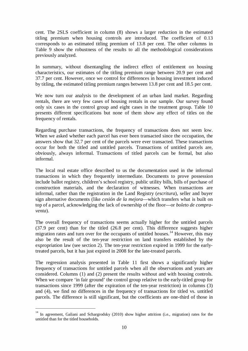
Some families, of course, have left the neighbourhood after treatment. Galiani and Schargrodsky (2010), which analyzed the effects of titles on household characteristics, had to deal with this issue of attrition and focused, necessarily, on the non-attrited families. For this study, the process of attrition is actually one of the outcomes of interest. Thus, we do not drop from the sample the parcels where the occupants have changed over time. On the contrary, our questionnaire asked carefully from these households whether they purchased, rented, squatted, inherited, etc. and whether they completed the necessary legal procedures for these transactions. In addition to the questionnaire on housing and household characteristics, we designed a complementary questionnaire to measure parcel valuations. This questionnaire was filled by the owners of a local real estate agency working in this area and provides a valuation of the dwellings at the parcel level.9 446 out of 448 valuations were successfully performed (the valuation was not performed in the San Martin parcels). In addition to the survey, we also obtained information from the Land Undersecretary of the Province of Buenos Aires on the legal status and ownership of each titled parcel as of 2007. By comparing the data we obtained in the field, relative to the legal registered information, we are able to precisely describe the process of de-regulation. In particular, we are able to compare the name of the current household members and whom the parcel is titled to. Our survey also asked for an explanation when the names differed. Thus, the analysis of deregularization compares de facto vs. de jure ownership information.

4. Methodology

Our first objective is to measure the titling transfer premium: the difference in real estate value between titled and untitled properties. In order to identify the effect of legal property rights on housing valuations we exploit a natural experiment in the allocation of land titling. In a natural experiment, like in a randomized trial, there is a control group that estimates what would have happened to the treated group in the absence of the intervention, but nature or other exogenous forces determine treatment status instead. The validity of the control group is evaluated by examining the exogeneity of treatment status with respect to the potential outcomes, and by testing that the pre-intervention characteristics of the treatment and control groups are reasonably similar. In section 2 we discussed at length the process of allocation of land title offers and argued that this process was exogenous to the characteristics of the parcels and squatters in our experiment. We now show the similarity of pre-treatment characteristics between the treatment and control groups. In Table 1, we compare pre-treatment characteristics for the non-intention-to-treat and intention-to-treat groups to analyze the presence of potential differences. The variable property right offer equals 1 for the parcels that were surrendered by the original owners, and 0 otherwise. In panel A, we compare parcel characteristics: distance to a nearby (polluted and floodable) creek, distance to the closest non-squatted area, parcel size, and a dummy for whether the parcel is located in a corner of a block. We only

9 This local real estate agency is located within this area and has operated since 1993. They know the titling status of the parcels and provided a valuation in Argentine pesos of each parcel.

7

reject the hypotheses of equality for parcel size (at the 8.9 per cent level of significance). Nevertheless, the difference in average parcel sizes between these two groups is relatively small—parcels are only 3 per cent larger in the non-intention-to-treat group—and if something, it is the control group that inhabits slightly larger parcels. In panel B of Table 1, we compare pre-treatment characteristics of the ‘original squatter’ between the non-intention-to-treat and intention-to-treat groups for the families that arrived before treatment. We define the ‘original squatter’ as the household head at the time the family arrived to the parcel they are currently occupying. We cannot reject the hypotheses of equality in age, gender, nationality and years of education of the original squatter, suggesting a strong similarity between these groups at the time of their arrival to this area. Moreover, we do not reject the hypotheses of equality in nationality and years of education of the mother and father of the original squatter across the groups, suggesting that these groups had been showing similar trends in their socio-economic development before their arrival to this area. The similarity across pre-treatment characteristics is consistent with the exogeneity in the allocation of property rights described above. Once treatment status has been shown to be exogenous, we analyze the effect of land titling on variable Y by estimating the following regression model:

iiii εβγα +++= X RightProperty Y (1)

where Y is any of the outcomes under study, and γ is the parameter of interest, which captures the causal effect of property right (a dummy variable that equals 1 for the squatters that received property titles, and 0 otherwise) on the outcome under consideration. X is a vector of exogenous parcel characteristics, and ε is the error term.10 However, when Y is housing valuation, the parameter γ would capture the overall effect of titling on housing value. Part of that effect would be the titling premium: a similar house is expected to be worth more when titled. But part of the effect could also come from differences in housing investments. Households may invest more in titled parcels. The titling premium is not just the difference in valuation between these two houses because we actually want to compare a similar house with and without title, and titled houses are likely to be better. Thus, for the estimation of the titling premium we will control not only for exogenous parcel characteristics affecting valuation (parcel surface, distance to creek, on the creek, block corner, distance to non-squatted area, distance to avenue, distance to pavement, on the pavement), but we will later add controls for housing investment characteristics also driven by titling. In particular, the variable overall housing appearance is an overall evaluation of the quality of the house. Moreover, specific housing characteristics are additionally captured by good roof, good walls, two-storey building, concrete sidewalk, and constructed area ratio. 10 As our unit of observation for this study is the parcel, regardless of whether the occupying family has changed over time, we do not control here for the individual characteristics of the original squatter (see Galiani and Schargrodsky 2010).

8

We perform this estimation of the titling premium using the valuations provided by the local real estate agency. One concern with housing valuations is that there are a few large outliers. We first exclude from the sample the upper 5 per cent of the valuation distribution and then perform a variety of robustness analyses including the whole sample, median regression, and robust regression. Another concern when conducting statistical inference is that the errors might not be independent across parcels. In particular, similar local shocks can affect investments by close neighbour families. In order to control for this potential nuisance, we also compute robust standard errors by clustering the parcels located in the same (rectangular) block. These standard errors are also robust to lack of homoskedasticity in the error term. To this point, our model has assumed that all the squatters actually received the treatment to which they were assigned. In many experiments, however, a portion of the participants fail to follow the treatment protocol, a problem termed treatment non-compliance. In our case, this might be of potential concern since a number of families that were offered the possibility of obtaining land titles did not receive them for reasons that may also affect their outcomes. In order to address this problem of non-compliance, we also report the reduced-form estimates from regressing the outcomes of interest on the intention-to-treat property right offer variable, a dummy indicating the availability of land title offers, and also the 2SLS estimates of the treatment effects from instrumenting the property right variable with the property right offer variable. In addition to the analysis of the titling transfer premium, we also measure differences in housing characteristics associated to titling. In particular, we consider the same values used later as controls in the titling premium estimates (overall housing appearance, good roof, good walls, two-storey building, concrete sidewalk, and constructed area ratio). Applying the same methodology, we also study whether titling facilitates the development of an urban real estate market considering as dependent variables the history of real estate transactions and mortgage credit, and the presence of rental transactions.

5. Regression results

We start the estimation of the titling premium in Table 2. The dependent variable is the valuation provided by the local real estate office considering the availability of titles for the titled parcels, and the lack of titles for the untitled parcels. Remember that the valuators knew the titling status of each parcel. To avoid the results being driven by the presence of some large outliers in the valuation sample, we first exclude from the analysis the observations in the upper 5 per cent of the valuation distribution.11 Using OLS and controlling for exogenous parcel characteristics (parcel surface, distance to creek, on the creek, block corner, distance to non-squatted area, distance to avenue, distance to pavement, on the pavement), column (1) shows a statistically strong effect of

11 The average valuation in our sample is AR$50,195 (about US$12,500). The 95th percentile corresponds to AR$88,796. The largest valuation is AR$242,000.

9

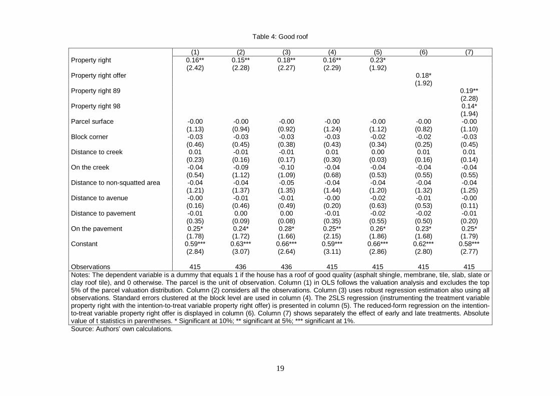
titles on parcel valuation. The estimated coefficient of 0.19 in a log equation on a binary regressor corresponds to an estimated titling premium of 20.9 per cent.12 A similar effect is obtained in the regression in levels in column (2). Column (3) shows a somewhat larger coefficient when the whole sample is considered (without restricting outliers). Columns (4) and (5) provide similar results for the whole sample addressing the presence of outliers with median and robust regression, respectively. Statistical significance shows no change in column (6) when standard errors are clustered at the block level to take into account potential correlation of the error term across neighbours. The 2SLS estimate in column (7), which considers the presence of non-compliers, provides a higher estimation of the titling premium. The coefficient reaches 0.32, which corresponds to a premium of 37.7 per cent. In reduced form, column (8) also addresses non-compliance giving an estimated coefficient of 0.25. Finally, column (9) suggests no difference in the effect of titling for early- vs. late-treated parcels. However, the problem with these regressions is that the estimation of the effect of titles on parcel valuation confuses the direct effect of titles (the difference in value for a similar house with and without titles) with the indirect effect from the increase in housing investment encouraged by titles. We need to introduce controls for housing quality differences to isolate the titling premium. Before doing that, we show in Tables 3 to 8 that there are indeed significant differences in housing quality associated to titling. In Table 3, the variable overall housing appearance summarizes the overall aspect of each house using an index from 0 to 100 points assigned by surveyors. The coefficient shows a significant effect of land titling on housing quality. Looking at individual housing characteristics, Tables 4 to 8 show significant differences in the quality of the roof, the constructed surface, and the presence of sidewalks made of concrete. The effects are weaker for the quality of the walls and the presence of two-storey buildings, but the coefficients are always positive confirming our previous results of statistically significant differences in housing investment associated to entitlement.13 Controlling for investment in housing characteristics, Table 9 repeats the analysis of Table 2. In column (1) we first control only for overall housing appearance (which shows a significant effect on valuation). In column (2) we also introduce the other housing controls (good roof, good walls, two-storey building, concrete sidewalk, and constructed area ratio). Good roof, good walls, and constructed area ratio show significant effects on valuation, in addition to overall housing appearance. As expected, Table 9 shows a reduction in the effect of titles on housing valuation estimated in Table 2, once housing controls are introduced. The OLS coefficient in column (2) is now 0.17, which corresponds to an estimated titling premium of 18.5 per

12 The percentage effect from the estimated coefficient γ on a binary regressor is calculated as

1% −=Δ γe . 13 These results do not need to coincide exactly with our previous results in Galiani and Schargrodsky (2010). Besides the fact that seven more years have elapsed, that paper looks at the effect of titling on households, focusing only on non-attrited families that remained in the same parcel since the original assignment of treatment (before 1986). The parcel is the unit of observation of this new study, regardless of whether the occupying family has changed or not over time.

10

cent. The 2SLS coefficient in column (8) shows a larger reduction in the estimated titling premium when housing controls are introduced. The coefficient of 0.13 corresponds to an estimated titling premium of 13.8 per cent. The other columns in Table 9 show the robustness of the results to all the methodological considerations previously analyzed. In summary, without disentangling the indirect effect of entitlement on housing characteristics, our estimates of the titling premium range between 20.9 per cent and 37.7 per cent. However, once we control for differences in housing investment induced by titling, the estimated titling premium ranges between 13.8 per cent and 18.5 per cent. We now turn our analysis to the development of an urban land market. Regarding rentals, there are very few cases of housing rentals in our sample. Our survey found only six cases in the control group and eight cases in the treatment group. Table 10 presents different specifications but none of them show any effect of titles on the frequency of rentals. Regarding purchase transactions, the frequency of transactions does not seem low. When we asked whether each parcel has ever been transacted since the occupation, the answers show that 32.7 per cent of the parcels were ever transacted. These transactions occur for both the titled and untitled parcels. Transactions of untitled parcels are, obviously, always informal. Transactions of titled parcels can be formal, but also informal. The local real estate office described to us the documentation used in the informal transactions in which they frequently intermediate. Documents to prove possession include ballot registry, children’s school registry, public utility bills, bills of purchase of construction materials, and the declaration of witnesses. When transactions are informal, rather than the registration in the Land Registry (escritura), seller and buyer sign alternative documents (like cesión de la mejora—which transfers what is built on top of a parcel, acknowledging the lack of ownership of the floor—or boleto de compra-venta). The overall frequency of transactions seems actually higher for the untitled parcels (37.9 per cent) than for the titled (26.8 per cent). This difference suggests higher migration rates and turn over for the occupants of untitled houses.14 However, this may also be the result of the ten-year restriction on land transfers established by the expropriation law (see section 2). The ten-year restriction expired in 1999 for the early-treated parcels, but it has just expired in 2008 for the late-treated parcels. The regression analysis presented in Table 11 first shows a significantly higher frequency of transactions for untitled parcels when all the observations and years are considered. Columns (1) and (2) present the results without and with housing controls. When we compare ‘in fair ground’ the control group relative to the early-titled group for transactions since 1999 (after the expiration of the ten-year restriction) in columns (3) and (4), we find no differences in the frequency of transactions for titled vs. untitled parcels. The difference is still significant, but the coefficients are one-third of those in

14 In agreement, Galiani and Schargrodsky (2010) show higher attrition (i.e., migration) rates for the untitled than for the titled households.

11

columns (1) and (2), when we introduce again the late-titled parcels in columns (5) and (6), but only for transactions since 2008 (when the ten-year rule had also expired for this group). In summary, there are both formal and informal transactions in this area, but without any evidence suggesting that titling increases the frequency of transactions.15 Finally, we also analyze in this section whether titling encourages the development of a mortgaged land market, improving access to credit. In agreement with previous results in Galiani and Schargrodsky (2010), we find a statistically significant difference in the access to mortgage credit in favour of the early-titled group (which given the ten-year restriction in the expropriation law qualifies for mortgages since 1999). The regression analysis is presented in Table 12. The differences become significant only when we split treatment between early and late titles in columns (9) and (10). Still, the frequency of mortgages is very low. The survey shows only six cases in which early-titled parcels received mortgaged credit. There are no cases for the late-titled or for the control group.

6. The deregularization process

We know all these parcels were occupied at the very same time in 1981. We also know the exact year titles were awarded (1989 for the early-treated parcels in the contiguous area, 1991 for the non-contiguous San Martin neighbourhood, and 1998 for the late-treated parcels in the contiguous area).16 The law also established that the squatters could not transfer the property of the parcels for the first ten years after titling (although our survey shows there were informal land transfers of titled parcels before the 10-year restriction). For both early and late-titled parcels, we had the detailed information on legal ownership from the Undersecretary of Land of the Province of Buenos Aires at the time of entitlement and as of 2007. Moreover, our survey asked 368 intention-to-treat households the identity of the current occupants of the houses, in particular, we asked who are considered now the ‘real’ owners of the parcel. When the original and the current owners differ, the survey follows a series of questions aiming to understand the reasons for these differences (formal transfers, informal transfers, death without inheritance processes, divorce, separation without divorce, indivisibilities among family members, further squatting, etc.). The analysis, in the form of a decision tree, is presented in Figure 1. In 63 per cent of the cases (232 cases), there was no change in ownership since titling. Within the other 136 cases, in 97 cases there are changes in ownership within the same family, and 39 changes of family. The 97 intra-family cases break down to: 72 changes in ownership upon death, 23 changes upon divorce, and 2 due to other reasons. When our surveyed were asked whether families followed the necessary legal steps to legally transfer ownership in these cases, legal procedures were followed in only 13.9 per cent (10 changes) of the

15 As expected, transactions are more frequent in the control group when we restrict only to informal transactions (using the classification developed for the deregularization analysis of section 6). All results reported but not presented are available from the authors upon request. 16 In order to enlarge the number of observations, we included San Martin to this deregularization analysis.

12

death cases, 26.1 per cent (6 changes) of the divorce cases, and one of the other cases. Thus, 82.5 per cent of the intra-family transactions did not complete legal procedures. Regarding the 39 cases of change in owner family, 33 are declared as purchases and 6 cases of squatting. Only 13 of the 33 cases of purchases (40 per cent) were legally completed. Thus, almost two-thirds of the inter-family ownership changes are not formalized. Considering both intra- and inter-family ownership changes, only a few years after legal titling, in 28.8 per cent of the parcels legal owners do not coincide with real owners. Figure 2 summarizes this information picturing in blue the percentages of regularized cases and in red the percentages of deregularization cases. Figures 3 and 4 break down the same analysis into the early-treated families, who received the titles in 1989-91, and the late-treated, who received the titles in 1998. As expected, there is a larger share of deregularized cases for the early-treated, as more time has elapsed since titling. Almost one-third (32.95 per cent) of the early-titled parcels are now deregularized, whereas the same figure represents one quarter (25 per cent) for the late-titled.

7. Conclusions

We exploit a natural experiment to estimate the titling premium: the difference in market value for a similar house with vs. without legal titles. Our estimates do not just compare the average value of titled and untitled houses because titling also fosters investment. When controlling for housing characteristics, our estimates hinge around 18.5 per cent. We also confirm that titling incentives investment. On the other hand, titling does not seem to encourage a rental and purchase land market. Titling is positively related to access to mortgage credit, but credit access is still very low. We also exploit this natural experiment to study the potential process of deregularization. 28.8 per cent of the titled parcels seem to have now become deregularized due to unregistered intra-family transactions (death, divorce, others) or inter-family transactions (informal sales, occupation, etc.). The figure seems surprisingly high given that these families have fought tenaciously for legal land ownership and our previous papers (Galiani and Schargrodsky 2004, 2010) and literature on other cases show strong positive effects from legal titling. Why do families become deregularized? Is it worth remaining formal? A main possible explanation is that the legal costs of remaining formal seem to be quite high for the low value of these parcels (and the low income of these families). We estimated the titling premium at 18.5 per cent. The average value of parcels in our sample is AR$46,824 (about US$11,700), which gives a titling premium of about US$2,164. We asked lawyers operating in Quilmes County on the costs of legal transactions. These legal transactions involve a variable cost, which depends on asset value, and a fixed cost. The cost of an inheritance process for an asset of US$11,700 is about US$2,300. The cost of the legal purchase procedure for this asset is about US$3,184. The cost of legal divorce for this asset is about US$2,440. Moreover, a family might need to incur these costs more than once over time. Thus, one possibility

13

is that the (potentially repeated) costs of remaining formal are too high for the low value of these parcels and the titling premium. These legal costs are also high relative to the income levels of these households. The average monthly household head income in our survey is AR$1,277 (about US$320), and the average total household income is AR$1,763 (about US$440). Thus, these poor families may not be able to afford legality. A similar argument may explain the low access to mortgage credit. The cost of eviction and mortgage execution for an asset of this value is about US$2,810 according to Quilmes lawyers. These high legal costs might also preclude mortgaged credit (together, of course, with the difficulties faced by this population to comply with the requirements of formal documentation and formal employment with significant tenure and high wages). The high costs of eviction probably also preclude rentals, making little difference between titled and untitled parcels in the possibility of renting. Similarly, the high costs of legal purchase transactions may also again explain why titling does not appear to have make a difference for the development of a real estate market in this urban poor area. In sum, a large fraction of households that enter a node at which formalization is challenged end up being (at least temporarily) deregularized. This seems to be the result of the high transaction costs involved in maintaining formalization (relative to the income of these households and the premium associated to land titling). Given that the high social benefits of land titling might get lost over time, a straightforward policy recommendation is that policy makers and regulators should aim to reduce and subsidize the costs of these legal transactions for these poor families.

14

References

Alchian, A., and H. Demsetz (1973). ‘The Property Rights Paradigm’. Journal of Economic History, 33(1): 16–27.

Alston, L., G. Libecap, and R. Schneider (1996). ‘The determinants and impact of property rights: land titles on the Brazilian frontier’. Journal of Law, Economics & Organization, 12: 25–61.

Banerjee, A., P. Gertler, and G. Maitreesh (2002). ‘Empowerment and Efficiency: Tenancy Reform in West Bengal’, Journal of Political Economy, 110(2): 239–80.

Besley, T. (1995). ‘Property Rights and Investments Incentives: Theory and Evidence from Ghana’. Journal of Political Economy, 103: 903–37.

Brasselle, A.-S., F. Gaspart, and J-P. Platteau (2002). ‘Land Tenure Security and Investment Incentives: Puzzling Evidence from Burkina Faso’. Journal of Development Economics, 67(2): 373–418.

Briante, M. (1982). ‘Las Tierras para el Hombre’, in El Porteño, reprinted in M. Briante (2004), Desde este mundo, Buenos Aires: Sudamericana.

Carter, M., and P. Olinto (2003). ‘Getting Institutions Right for Whom? Credit Constraints and the Impact of Property Rights on the Quantity and Composition of Investment’. American Journal of Agricultural Economics, 85: 173–86.

Cespedes, M. (1984). ‘Por una Tierra Nuestra’. Documentary movie.

CEUR (1984). Condiciones de Habitat y Salud de los Sectores Populares. Un Estudio Piloto en el Asentamiento San Martín de Quilmes. Buenos Aires: Centro de Estudios Urbanos y Regionales.

De Long, J.B., and A. Shleifer (1993). ‘Princes and Merchants: European City Growth before the Industrial Revolution’. Journal of Law and Economics, 36(2): 671–702.

Demsetz, H. (1967). ‘Toward a Theory of Property Rights’. American Economic Review, 57(2): 347–59.

De Soto, H. (2000). The Mystery of Capital: Why Capitalism Triumphs in the West and Fails Everywhere Else. New York: Basic Books.

Di Tella, R., S. Galiani, and E. Schargrodsky (2007). ‘The Formation of Beliefs: Evidence from the Allocation of Land Titles to Squatters’, Quarterly Journal of Economics, 122(1): 209–41.

Do, Q-T., and L. Iyer (2008). ‘Land Titling and Rural Transition in Vietnam’. Economic Development and Cultural Change, 56(3): 531–79.

Fara, L. (1989). ‘Luchas Reivindicativas Urbanas en un Contexto Autoritario. Los Asentamientos de San Francisco Solano’. In E. Jelin (ed.), Los Nuevos Movimientos Sociales. Buenos Aires: Centro Editor de América Latina.

Feder, G., T. Onchan, Y. Chalamwong, and C. Hongladarom (1988). Land Policies and Farm Productivity in Thailand. Baltimore: Johns Hopkins University Press.

15

Field, E. (2005). ‘Property Rights and Investment in Urban Slums’. Journal of the European Economic Association, 3(2-3): 279–90.

Field, E. (2007). ‘Entitled to Work: Urban Property Rights and Labor Supply in Peru’. Quarterly Journal of Economics, 122(4): 1561–602.

Field, E., and M. Torero (2003). ‘Do Property Titles Increase Credit Access among the Urban Poor? Evidence from a Nationwide Titling Program in Peru’. Mimeo, Princeton University.

Galiani, S., and E. Schargrodsky (2004). ‘Effects of Land Titling on Child Health’, Economics and Human Biology, 2(3): 353–72.

Galiani, S., and E. Schargrodsky (2010). ‘Property Rights for the Poor: Effects of Land Titling’, Journal of Public Economics, 94(9-10): 700–29.

Izaguirre, I., and Z. Aristizabal (1988). Las Tomas de Tierras en la Zona Sur del Gran Buenos Aires. Un Ejercicio de Formación de Poder en el Campo Popular. Buenos Aires: Centro Editor de América Latina.

Jimenez, E. (1984). ‘Tenure security and urban squatting’. REStat 66: 556–67.

Lanjouw, J., and P. Levy (2002). ‘Untitled: a study of formal and informal property rights in urban Ecuador’. Economic Journal, 112: 986–1019.

Libecap, G., and D. Lueck (2008). ‘The Demarcation of Land: Patterns and Economic Effects’. Mimeo, UCSD.

North, D. (1981). Structure and Change in Economic History. New York: Norton.

North, D., and R. Thomas (1973). The Rise of the Western World: A New Economic History. New York: Cambridge University Press.

Place, F., and S. Migot-Adholla (1998). ‘The Economic Effects of Land Registration for Smallholder Farms in Kenya: Evidence from Nyeri and Kakamega Districts’. Land Economics, 74(3): 360–73.

Vogl, T. (2007). ‘Urban Land Rights and Child Nutritional Status in Peru’. Economics & Human Biology, 5(2): 302–21.

16

Table 1: Pre-treatment characteristics

Property right offer=0

Property right offer=1 Difference

A. Characteristics of the parcel Distance to creek (in blocks)

1.995 (0.061)

1.906 (0.034)

0.088 (0.070)

Distance to non-squatted area (in blocks)

1.731 (0.058)

1.767 (0.033)

-0.036 (0.067)

Parcel size (in squared meters)

287.219 (4.855)

277.662 (2.799)

9.556* (5.605)

Block corner=1 0.190 (0.019)

0.156 (0.014)

0.033 (0.023)

B. Characteristics of the original squatter

Age 48.875 (0.938)

50.406 (0.761)

-1.532 (1.208)

Female=1 0.407 (0.046)

0.353 (0.035)

0.054 (0.058)

Argentine=1 0.903 (0.028)

0.904 (0.022)

-0.001 (0.035)

Years of education 6.071 (0.188)

5.995 (0.141)

0.076 (0.235)

Argentine father=1 0.795 (0.038)

0.866 (0.025)

-0.072 (0.046)

Years of education of the father

4.655 (0.147)

4.417 (0.076)

0.237 (0.165)

Argentine mother=1 0.804 (0.038)

0.856 (0.026)

-0.052 (0.046)

Years of education of the mother

4.509 (0.122)

4.548 (0.085)

-0.039 (0.149)

Source: Galiani and Schargrodsky (2010). Standard errors are in parentheses. * Significant at 10 per cent.

17

Table 2: Parcel valuation

(1) (2) (3) (4) (5) (6) (7) (8) (9) Property right 0.19*** 7738.79*** 0.21*** 0.23*** 0.21*** 0.19*** 0.32*** (3.62) (3.40) (3.74) (3.23) (3.72) (2.81) (3.29) Property right offer 0.25*** (3.30) Property right 89 0.17** (2.49) Property right 98 0.20*** (3.51) Parcel surface -0.00 -7.84 -0.00 -0.00 -0.00 -0.00 -0.00 -0.00 -0.00 (0.65) (0.73) (0.56) (0.43) (0.72) (0.44) (0.63) (0.13) (0.67) Block corner -0.03 58.16 -0.01 -0.04 -0.01 -0.03 -0.01 -0.01 -0.03 (0.50) (0.02) (0.14) (0.54) (0.25) (0.37) (0.25) (0.09) (0.51) Distance to creek 0.03 1208.01 0.00 0.03 0.01 0.03 0.01 0.02 0.03 (0.69) (0.69) (0.11) (0.54) (0.35) (0.66) (0.24) (0.47) (0.75) On the creek -0.26*** -9080.88*** -0.34*** -0.29*** -0.31*** -0.26*** -0.26*** -0.26*** -0.26*** (4.02) (3.27) (4.91) (3.39) (4.45) (3.26) (3.97) (4.03) (4.00) Distance to non-squatted area -0.02 -944.65 -0.01 0.02 -0.01 -0.02 -0.02 -0.03 -0.02 (0.87) (0.91) (0.54) (0.51) (0.30) (0.68) (0.85) (1.07) (0.82) Distance to avenue -0.04** -1815.44** -0.05*** -0.05** -0.05*** -0.04** -0.06*** -0.06** -0.04** (2.16) (2.47) (2.79) (2.41) (2.87) (2.42) (2.64) (2.57) (2.19) Distance to pavement -0.06** -2596.12** -0.05** -0.07** -0.06** -0.06** -0.07*** -0.07*** -0.06** (2.50) (2.55) (2.04) (2.18) (2.31) (2.13) (2.85) (2.79) (2.55) On the pavement 0.11 6102.65 0.08 0.05 0.09 0.11 0.13 0.09 0.10 (0.94) (1.26) (0.65) (0.32) (0.74) (1.07) (1.14) (0.81) (0.92) Constant 11.10*** 66487.56*** 11.21*** 11.17*** 11.23*** 11.10*** 11.23*** 11.17*** 11.11*** (66.46) (9.24) (62.72) (49.69) (62.14) (65.65) (59.66) (62.96) (66.18) Observations 415 415 436 436 436 415 415 415 415 Notes: The dependent variable is the natural log of the parcel valuation in AR$ assigned by the local real estate office. The parcel is the unit of observation. Column (1) in OLS excludes the top 5% of the parcel valuation distribution. In column (2) the dependent variable is measured in levels. Column (3) considers all the observations. Column (4) and column (5) use median and robust regression estimation, respectively, using all observations. Standard errors clustered at the block level are used in column (6). The 2SLS regression (instrumenting the treatment variable property right with the intention-to-treat variable property right offer) is presented in column (7). The reduced-form regression on the intention-to-treat variable property right offer is displayed in column (8). Column (9) shows separately the effect of early and late treatments. Absolute value of t statistics in parentheses. * Significant at 10%; ** significant at 5%; *** significant at 1%. Source: Authors’ own calculations.

18

Table 3: Overall housing appearance

(1) (2) (3) (4) (5) (6) (7) (8) Property right 4.19* 4.29* 2.66 3.99 4.19 9.69** (1.68) (1.73) (0.59) (1.53) (1.45) (2.09) Property right offer 7.58** (2.11) Property right 89 5.19 (1.61) Property right 98 3.64 (1.33) Parcel surface -0.02 -0.02 -0.03 -0.02 -0.02 -0.02 -0.01 -0.02 (1.39) (1.31) (1.44) (1.53) (1.48) (1.33) (1.05) (1.37) Block corner -1.46 -0.22 -0.95 -0.07 -1.46 -0.81 -0.62 -1.45 (0.55) (0.08) (0.20) (0.03) (0.47) (0.30) (0.23) (0.55) Distance to creek 0.88 0.71 0.18 0.63 0.88 0.12 0.42 0.75 (0.46) (0.39) (0.05) (0.32) (0.41) (0.06) (0.22) (0.39) On the creek 0.35 -0.84 -4.65 -1.11 0.35 0.33 0.36 0.34 (0.11) (0.28) (0.86) (0.35) (0.12) (0.11) (0.12) (0.11) Distance to non-squatted area 0.01 0.34 0.11 0.07 0.01 -0.01 -0.11 -0.04 (0.01) (0.30) (0.05) (0.06) (0.01) (0.01) (0.10) (0.03) Distance to avenue -0.23 -0.39 0.09 -0.32 -0.23 -1.36 -1.22 -0.20 (0.29) (0.50) (0.06) (0.38) (0.29) (1.20) (1.14) (0.25) Distance to pavement -1.38 -1.05 -2.33 -1.10 -1.38 -1.86 -1.83 -1.25 (1.23) (0.95) (1.16) (0.95) (1.01) (1.58) (1.58) (1.09) On the pavement 0.51 0.56 -4.63 -1.44 0.51 1.57 0.41 0.58 (0.10) (0.11) (0.50) (0.26) (0.10) (0.29) (0.08) (0.11) Constant 54.46*** 54.42*** 62.35*** 56.14*** 54.46*** 59.90*** 58.12*** 54.10*** (6.99) (7.03) (4.46) (6.87) (4.97) (6.86) (7.04) (6.90) Observations 403 423 423 423 403 403 403 403 Notes: The dependent variable measures the overall aspect of each house from 0 to 100 points assigned by the surveyors assuming 0 for the worst dwelling in a shanty town of Solano and 100 for a middle-class house in downtown Quilmes (the main locality of the county). The parcel is the unit of observation. Column (1) in OLS follows the valuation analysis and excludes the top 5% of the parcel valuation distribution. Column (2) considers all the observations. Column (3) and column (4) use median and robust regression estimation, respectively, using all observations. Standard errors clustered at the block level are used in column (5). The 2SLS regression (instrumenting the treatment variable property right with the intention-to-treat variable property right offer) is presented in column (6). The reduced-form regression on the intention-to-treat variable property right offer is displayed in column (7). Column (8) shows separately the effect of early and late treatments. Absolute value of t statistics in parentheses. * Significant at 10%; ** significant at 5%; *** significant at 1%.

Source: Authors’ own calculations.

19

Table 4: Good roof

(1) (2) (3) (4) (5) (6) (7) Property right 0.16** 0.15** 0.18** 0.16** 0.23* (2.42) (2.28) (2.27) (2.29) (1.92) Property right offer 0.18* (1.92) Property right 89 0.19** (2.28) Property right 98 0.14* (1.94) Parcel surface -0.00 -0.00 -0.00 -0.00 -0.00 -0.00 -0.00 (1.13) (0.94) (0.92) (1.24) (1.12) (0.82) (1.10) Block corner -0.03 -0.03 -0.03 -0.03 -0.02 -0.02 -0.03 (0.46) (0.45) (0.38) (0.43) (0.34) (0.25) (0.45) Distance to creek 0.01 -0.01 -0.01 0.01 0.00 0.01 0.01 (0.23) (0.16) (0.17) (0.30) (0.03) (0.16) (0.14) On the creek -0.04 -0.09 -0.10 -0.04 -0.04 -0.04 -0.04 (0.54) (1.12) (1.09) (0.68) (0.53) (0.55) (0.55) Distance to non-squatted area -0.04 -0.04 -0.05 -0.04 -0.04 -0.04 -0.04 (1.21) (1.37) (1.35) (1.44) (1.20) (1.32) (1.25) Distance to avenue -0.00 -0.01 -0.01 -0.00 -0.02 -0.01 -0.00 (0.16) (0.46) (0.49) (0.20) (0.63) (0.53) (0.11) Distance to pavement -0.01 0.00 0.00 -0.01 -0.02 -0.02 -0.01 (0.35) (0.09) (0.08) (0.35) (0.55) (0.50) (0.20) On the pavement 0.25* 0.24* 0.28* 0.25** 0.26* 0.23* 0.25* (1.78) (1.72) (1.66) (2.15) (1.86) (1.68) (1.79) Constant 0.59*** 0.63*** 0.66*** 0.59*** 0.66*** 0.62*** 0.58*** (2.84) (3.07) (2.64) (3.11) (2.86) (2.80) (2.77) Observations 415 436 436 415 415 415 415 Notes: The dependent variable is a dummy that equals 1 if the house has a roof of good quality (asphalt shingle, membrane, tile, slab, slate or clay roof tile), and 0 otherwise. The parcel is the unit of observation. Column (1) in OLS follows the valuation analysis and excludes the top 5% of the parcel valuation distribution. Column (2) considers all the observations. Column (3) uses robust regression estimation also using all observations. Standard errors clustered at the block level are used in column (4). The 2SLS regression (instrumenting the treatment variable property right with the intention-to-treat variable property right offer) is presented in column (5). The reduced-form regression on the intention-to-treat variable property right offer is displayed in column (6). Column (7) shows separately the effect of early and late treatments. Absolute value of t statistics in parentheses. * Significant at 10%; ** significant at 5%; *** significant at 1%.

Source: Authors’ own calculations.

20

Table 5: Good walls

(1) (2) (3) (4) (5) (6) (7) Property right 0.08 0.10 0.12 0.08 0.16 (1.32) (1.54) (1.50) (1.31) (1.39) Property right offer 0.13 (1.39) Property right 89 0.09 (1.08) Property right 98 0.08 (1.17) Parcel surface -0.00** -0.00** -0.00** -0.00** -0.00** -0.00** -0.00** (2.42) (2.18) (2.24) (2.31) (2.40) (2.17) (2.41) Block corner -0.04 -0.01 -0.02 -0.04 -0.03 -0.03 -0.04 (0.59) (0.15) (0.20) (0.60) (0.47) (0.40) (0.59) Distance to creek 0.01 -0.02 -0.02 0.01 -0.00 -0.00 0.01 (0.12) (0.40) (0.38) (0.13) (0.09) (0.00) (0.11) On the creek -0.05 -0.08 -0.11 -0.05 -0.05 -0.05 -0.05 (0.60) (1.08) (1.11) (0.61) (0.59) (0.61) (0.60) Distance to non-squatted area 0.01 0.01 0.00 0.01 0.01 0.00 0.01 (0.18) (0.19) (0.13) (0.19) (0.19) (0.10) (0.18) Distance to avenue 0.03 0.02 0.03 0.03* 0.02 0.02 0.03 (1.55) (0.87) (1.01) (1.89) (0.54) (0.67) (1.55) Distance to pavement -0.04 -0.04 -0.04 -0.04 -0.05* -0.05* -0.04 (1.51) (1.37) (1.27) (1.33) (1.68) (1.66) (1.46) On the pavement 0.06 0.06 0.06 0.06 0.08 0.06 0.06 (0.47) (0.45) (0.36) (0.60) (0.57) (0.43) (0.47) Constant 0.70*** 0.78*** 0.84*** 0.70*** 0.78*** 0.74*** 0.70*** (3.43) (3.90) (3.34) (3.03) (3.42) (3.46) (3.41) Observations 415 436 436 415 415 415 415 Notes: The dependent variable is a dummy that equals 1 if the house has walls of good quality (brick, stone, block or concrete with exterior siding), and 0 otherwise. The parcel is the unit of observation. Column (1) in OLS follows the valuation analysis and excludes the top 5% of the parcel valuation distribution. Column (2) considers all the observations. Column (3) uses robust regression estimation also using all observations. Standard errors clustered at the block level are used in column (4). The 2SLS regression (instrumenting the treatment variable property right with the intention-to-treat variable property right offer) is presented in column (5). The reduced-form regression on the intention-to-treat variable property right offer is displayed in column (6). Column (7) shows separately the effect of early and late treatments. Absolute value of t statistics in parentheses. * Significant at 10%; ** significant at 5%; *** significant at 1%.

Source: Authors’ own calculations.

21

Table 6: Concrete sidewalk

(1) (2) (3) (4) (5) (6) Property right 0.06 0.06 0.06 0.28*** (1.49) (1.47) (1.32) (3.52) Property right offer 0.22*** (3.69) Property right 89 -0.01 (0.16) Property right 98 0.10** (2.24) Parcel surface -0.00 -0.00 -0.00 -0.00 -0.00 -0.00 (1.32) (1.32) (0.99) (1.29) (0.76) (1.40) Block corner -0.09* -0.08* -0.09* -0.06 -0.05 -0.09** (1.92) (1.80) (1.87) (1.36) (1.23) (1.98) Distance to creek 0.02 0.03 0.02 -0.01 -0.00 0.03 (0.59) (0.93) (0.32) (0.33) (0.09) (0.88) On the creek -0.06 -0.05 -0.06 -0.06 -0.06 -0.06 (1.20) (0.93) (0.94) (1.15) (1.24) (1.16) Distance to non-squatted area -0.04** -0.04** -0.04* -0.04** -0.04** -0.04* (2.06) (2.36) (1.73) (1.98) (2.31) (1.89) Distance to avenue 0.06*** 0.06*** 0.06** 0.01 0.01 0.05*** (4.05) (4.27) (2.25) (0.48) (0.80) (3.87) Distance to pavement 0.02 0.01 0.02 -0.00 0.00 0.01 (0.97) (0.78) (0.73) (0.08) (0.02) (0.49) On the pavement -0.06 -0.07 -0.06 -0.02 -0.06 -0.07 (0.72) (0.84) (0.89) (0.24) (0.64) (0.78) Constant 0.65*** 0.65*** 0.65*** 0.88*** 0.82*** 0.68*** (4.87) (4.99) (3.43) (5.68) (5.86) (5.06) Observations 411 432 411 411 411 411 Notes: The dependent variable is a dummy that equals 1 if the house has a sidewalk made of concrete, and 0 otherwise. The parcel is the unit of observation. Column (1) in OLS follows the valuation analysis and excludes the top 5% of the parcel valuation distribution. Column (2) considers all the observations. Standard errors clustered at the block level are used in column (3). The 2SLS regression (instrumenting the treatment variable property right with the intention-to-treat variable property right offer) is presented in column (4). The reduced-form regression on the intention-to-treat variable property right offer is displayed in column (5). Column (6) shows separately the effect of early and late treatments. Absolute value of t statistics in parentheses. * Significant at 10%; ** significant at 5%; *** significant at 1%.

Source: Authors’ own calculations.

22

Table 7: Two-storey building

(1) (2) (3) (4) (5) (6) Property right 0.04 0.05 0.04 0.15 (0.71) (0.91) (0.66) (1.61) Property right offer 0.12 (1.63) Property right 89 0.15** (2.29) Property right 98 -0.03 (0.49) Parcel surface -0.00** -0.00 -0.00** -0.00** -0.00* -0.00* (2.05) (1.52) (2.21) (2.02) (1.76) (1.95) Block corner 0.01 0.00 0.01 0.02 0.02 0.01 (0.12) (0.05) (0.12) (0.34) (0.41) (0.18) Distance to creek -0.01 -0.04 -0.01 -0.03 -0.03 -0.03 (0.38) (0.94) (0.42) (0.75) (0.66) (0.75) On the creek -0.05 -0.11* -0.05 -0.05 -0.05 -0.06 (0.87) (1.76) (1.10) (0.85) (0.88) (0.95) Distance to non-squatted area -0.04* -0.04* -0.04 -0.04 -0.04* -0.04* (1.66) (1.69) (1.67) (1.63) (1.75) (1.89) Distance to avenue -0.01 -0.02 -0.01 -0.03 -0.03 -0.01 (0.60) (1.16) (0.55) (1.46) (1.44) (0.36) Distance to pavement -0.02 -0.01 -0.02 -0.03 -0.03 -0.00 (0.76) (0.53) (0.53) (1.17) (1.14) (0.15) On the pavement -0.03 -0.05 -0.03 -0.01 -0.03 -0.02 (0.28) (0.44) (0.26) (0.07) (0.25) (0.21) Constant 0.51*** 0.58*** 0.51*** 0.63*** 0.59*** 0.47*** (3.18) (3.50) (2.73) (3.48) (3.53) (2.95) Observations 415 436 415 415 415 415 Notes: The dependent variable is a dummy that equals 1 if the construction has more than one storey, and 0 otherwise. The parcel is the unit of observation. Column (1) in OLS follows the valuation analysis and excludes the top 5% of the parcel valuation distribution. Column (2) considers all the observations. Standard errors clustered at the block level are used in column (3). The 2SLS regression (instrumenting the treatment variable property right with the intention-to-treat variable property right offer) is presented in column (4). The reduced-form regression on the intention-to-treat variable property right offer is displayed in column (5). Column (6) shows separately the effect of early and late treatments. Absolute value of t statistics in parentheses. * Significant at 10%; ** significant at 5%; *** significant at 1%.

Source: Authors’ own calculations.

23

Table 8: Constructed surface

(1) (2) (3) (4) (5) (6) (7) (8) Property right 2.36 6.49 5.32 4.16 2.36 21.19*** (0.64) (1.53) (1.47) (1.08) (0.52) (3.05) Property right offer 16.50*** (3.18) Property right 89 1.48 (0.31) Property right 98 2.85 (0.71) Parcel surface 0.00 0.00 0.01 0.01 0.00 0.00 0.01 0.00 (0.10) (0.22) (0.48) (0.40) (0.09) (0.14) (0.62) (0.09) Block corner 0.60 1.22 1.15 3.00 0.60 2.55 3.13 0.58 (0.16) (0.28) (0.30) (0.75) (0.15) (0.63) (0.80) (0.15) Distance to creek 0.15 -1.69 1.52 -0.25 0.15 -2.41 -1.80 0.27 (0.05) (-0.53) (0.56) (0.09) (0.05) (0.80) (0.64) (0.09) On the creek -6.51 -11.29** -8.50* -11.08** -6.51 -6.40 -6.56 -6.47 (1.45) (2.21) (1.95) (2.38) (1.35) (1.38) (1.48) (1.44) Distance to non-squatted area -0.85 -0.66 1.96 -0.00 -0.85 -0.81 -1.15 -0.81 (0.51) (0.34) (1.20) (0.00) (0.39) (0.47) (0.70) (0.48) Distance to avenue -0.85 -2.84** -1.11 -1.40 -0.85 -4.76*** -4.41*** -0.88 (0.71) (2.10) (0.97) (1.14) (0.56) (2.76) (2.83) (0.74) Distance to pavement -3.65** -3.74** -3.78** -3.47** -3.65** -5.42*** -5.24*** -3.76** (2.22) (1.98) (2.37) (2.02) (2.25) (3.04) (3.11) (2.23) On the pavement -1.82 -3.76 -1.61 -0.70 -1.82 1.78 -0.79 -1.87 (0.23) (0.41) (0.21) (0.08) (0.43) (0.22) (0.10) (0.24) Constant 83.99*** 98.65*** 75.93*** 84.38*** 83.99*** 103.44*** 99.02*** 84.30*** (7.24) (7.38) (6.67) (6.94) (6.82) (7.72) (8.15) (7.23) Observations 415 436 436 436 415 415 415 415 Notes: The dependent variable is the constructed surface in squared meters. The parcel is the unit of observation. Column (1) in OLS follows the valuation analysis and excludes the top 5% of the parcel valuation distribution. Column (2) considers all the observations. Column (3) and Column (4) use median and robust regression estimation, respectively, using all observations. Standard errors clustered at the block level are used in column (5). The 2SLS regression (instrumenting the treatment variable property right with the intention-to-treat variable property right offer) is presented in column (6). The reduced-form regression on the intention-to-treat variable property right Offer is displayed in column (7). Column (8) shows separately the effect of early and late treatments. Absolute value of t statistics in parentheses. * Significant at 10%; ** significant at 5%; *** significant at 1%.

Source: Authors’ own calculations.

24

Table 9: Parcel valuation (1) (2) (3) (4) (5) (6) (7) (8) (9) (10) Property right 0.17*** 0.17*** 7187.71*** 0.15*** 0.14*** 0.13*** 0.17*** 0.13** (3.36) (4.75) (4.81) (4.11) (2.95) (3.84) (3.39) (1.99) Property right offer 0.10* (1.95) Property right 89 0.17*** (3.70) Property right 98 0.17*** (4.31) Parcel surface -0.00 0.00*** 82.40*** 0.00*** 0.00*** 0.00*** 0.00*** 0.00*** 0.00*** 0.00*** (-0.06) (9.37) (10.14) (9.32) (8.54) (10.63) (7.23) (9.31) (9.14) (9.35) Block corner -0.03 -0.05 -1028.67 -0.04 -0.06 -0.05 -0.05 -0.06 -0.05 -0.05 (-0.55) (-1.39) (0.66) (1.15) (1.21) (1.47) (1.24) (1.47) (1.32) (1.39) Distance to creek 0.02 0.02 1130.27 0.01 -0.00 0.00 0.02 0.03 0.03 0.02 (0.49) (0.87) (1.01) (0.38) (0.10) (0.08) (0.88) (1.01) (1.15) (0.86) On the creek -0.24*** -0.18*** -5522.40*** -0.21*** -0.18*** -0.18*** -0.18** -0.18*** -0.18*** -0.18*** (3.95) (4.11) (3.07) (4.84) (3.31) (4.51) (2.66) (4.09) (4.01) (4.10) Distance to non-squatted area -0.02 -0.01 -227.49 0.00 0.01 0.01 -0.01 -0.00 -0.01 -0.01 (1.00) (0.33) (0.33) (0.06) (0.61) (0.82) (0.28) (0.30) (0.38) (0.33) Distance to avenue -0.04** -0.04*** -1809.49*** -0.03*** -0.03** -0.04*** -0.04** -0.03** -0.03* -0.04*** (2.33) (3.37) (3.75) (2.76) (2.16) (3.51) (2.62) (2.01) (1.95) (3.35) Distance to pavement -0.05** -0.02 -971.60 -0.02 -0.03 -0.03** -0.02 -0.02 -0.02 -0.02 (2.15) (1.47) (1.46) (1.46) (1.51) (2.14) (1.15) (1.24) (1.24) (1.43) On the pavement 0.10 0.09 5689.00* 0.08 0.06 0.11 0.09 0.08 0.06 0.09 (0.96) (1.18) (1.84) (0.97) (0.61) (1.51) (0.86) (1.06) (0.81) (1.18) Good roof 0.09*** 3877.23*** 0.08** 0.08** 0.08*** 0.09*** 0.10*** 0.11*** 0.09*** (3.14) (3.10) (2.55) (2.03) (2.88) (3.07) (3.20) (3.51) (3.13) Good walls 0.10*** 3190.90** 0.09*** 0.07* 0.08*** 0.10*** 0.10*** 0.11*** 0.10*** (3.42) (2.56) (3.00) (1.92) (3.08) (2.86) (3.44) (3.46) (3.42) Two-storey building -0.03 -726.21 0.02 -0.01 -0.02 -0.03 -0.03 -0.03 -0.03 (0.70) (0.46) (0.54) (0.20) (0.72) (0.69) (0.70) (0.72) (0.70) Concrete sidewalk 0.04 1530.15 0.04 0.05 0.06 0.04 0.05 0.04 0.04 (1.04) (0.87) (0.90) (0.87) (1.59) (0.98) (1.11) (1.02) (1.03) Constructed area ratio 2.17*** 101217.83*** 2.04*** 2.43*** 2.40*** 2.17*** 2.16*** 2.11*** 2.17*** (17.22) (19.13) (17.93) (16.84) (23.61) (12.67) (17.00) (16.36) (17.18) Overall housing appearance 0.01*** 0.00*** 132.89*** 0.00*** 0.00*** 0.00*** 0.00*** 0.00*** 0.00*** 0.00*** (7.33) (4.54) (4.02) (5.64) (3.84) (5.50) (5.40) (4.57) (4.52) (4.54) Observations 403 399 399 419 419 419 399 399 399 399 Notes: The dependent variable is the natural log of the parcel valuation in AR$ assigned by the local real estate office. The parcel is the unit of observation. Column (1) in OLS excludes the top 5% of the parcel valuation distribution. In column (2) additional housing characteristics are incorporated as controls. In column (3) the dependent variable is measured in levels. Column (4) considers all the observations. Column (5) and column (6) use median and robust regression estimation, respectively, using all observations. Standard errors clustered at the block level are used in column (7). The 2SLS regression (instrumenting the treatment variable property right with the intention-to-treat variable property right offer) is presented in column (8). The reduced-form regression on the intention-to-treat variable property right offer is displayed in column (9). Column (10) shows separately the effect of early and late treatments. The constant is not presented. Absolute value of t statistics in parentheses. * Significant at 10%; ** significant at 5%; *** significant at 1%. Source: Authors’ own calculations.

25

Table 10: Rental cases (1) (2) (3) (4) (5) (6) (7) (8) (9) (10) Property right 0.01 0.01 0.01 0.01 -0.01 -0.01 (0.29) (0.46) (0.26) (0.42) (0.33) (0.20) Property right offer -0.01 -0.01 (0.33) (0.20) Property right 89 0.03 0.04 (1.17) (1.29) Property right 98 -0.01 -0.01 (0.38) (0.22) Parcel surface 0.00 0.00 0.00 0.00 0.00 0.00 0.00 0.00 0.00 0.00 (0.11) (0.59) (0.11) (0.52) (0.09) (0.58) (0.05) (0.57) (0.18) (0.64) Block corner 0.02 0.01 0.02 0.01 0.02 0.01 0.02 0.01 0.02 0.01 (0.78) (0.58) (0.67) (0.48) (0.67) (0.50) (0.66) (0.48) (0.81) (0.62) Distance to creek -0.00 0.00 -0.00 0.00 0.00 0.00 0.00 0.00 -0.00 -0.00 (0.01) (0.04) (0.01) (0.03) (0.15) (0.19) (0.13) (0.18) (0.22) (0.18) On the creek -0.01 -0.01 -0.01 -0.01 -0.01 -0.01 -0.01 -0.01 -0.01 -0.01 (0.23) (0.25) (0.23) (0.26) (0.23) (0.24) (0.23) (0.24) (0.23) (0.26) Distance to non-squatted area -0.02* -0.02* -0.02 -0.02* -0.02* -0.02* -0.02* -0.02* -0.02* -0.02** (1.78) (1.94) (1.58) (1.69) (1.76) (1.91) (1.75) (1.90) (1.92) (2.07) Distance to avenue 0.01 0.01 0.01 0.01 0.01 0.01 0.01 0.01 0.01 0.01 (0.90) (1.15) (0.72) (0.95) (1.05) (1.20) (1.07) (1.23) (1.04) (1.24) Distance to pavement 0.01 0.01 0.01 0.01 0.01 0.01 0.01 0.01 0.01 0.01 (0.51) (0.61) (0.44) (0.53) (0.65) (0.73) (0.65) (0.73) (0.85) (0.93) On the pavement -0.05 -0.05 -0.05*** -0.05** -0.05 -0.05 -0.05 -0.05 -0.05 -0.05 (0.98) (0.96) (2.91) (2.29) (1.05) (1.03) (1.03) (1.02) (0.94) (0.92) Good roof -0.01 -0.01 -0.01 -0.01 -0.01 (0.72) (0.77) (0.63) (0.67) (0.67) Good walls 0.00 0.00 0.00 0.00 0.00 (0.13) (0.15) (0.16) (0.16) (0.14) Two-storey building -0.02 -0.02 -0.02 -0.02 -0.02 (0.65) (0.74) (0.65) (0.65) (0.87) Concrete sidewalk -0.03 -0.03 -0.03 -0.03 -0.03 (1.12) (1.12) (1.05) (1.03) (0.96) Constructed area ratio 0.09 0.09 0.08 0.09 0.09 (1.19) (1.28) (1.17) (1.20) (1.22) Overall housing appearance -0.00 -0.00 -0.00 -0.00 -0.00 (0.16) (0.14) (0.13) (0.13) (0.20) Observations 423 419 423 419 423 419 423 419 423 419 Notes: The dependent variable is a dummy that equals 1 if a household is renting all or part of the parcel, and 0 otherwise. The parcel is the unit of observation. Columns (1) and (2) present the OLS regressions without and with controls for housing characteristics, respectively. Standard errors clustered at the block level are used in columns (3) and (4). The 2SLS regression (instrumenting the treatment variable property right with the intention-to-treat variable property right offer) is presented in columns (5) and (6). The reduced-form regression on the intention-to-treat variable property right offer is displayed in columns (7) and (8). Columns (9) and (10) show separately the effect of early and late treatments. The constant is not presented. Absolute value of t statistics in parentheses. * Significant at 10%; ** significant at 5%; *** significant at 1%.

Source: Authors’ own calculations.

26

Table 11: Ever transacted

(1) (2) (3) (4) (5) (6) Property right -0.15** -0.16*** -0.04 -0.04 -0.05* -0.05* (2.50) (2.60) (0.82) (0.71) (1.80) (1.77) Parcel surface -0.00*** -0.00*** 0.00 -0.00 0.00 0.00 (2.87) (2.95) (0.68) (0.24) (0.97) (0.65) Block corner -0.09 -0.08 -0.06 -0.05 -0.02 -0.01 (1.35) (1.19) (1.06) (0.94) (0.56) (0.44) Distance to creek 0.04 0.03 -0.01 -0.01 0.00 0.01 (0.85) (0.73) (0.24) (0.41) (0.22) (0.27) On the creek 0.12 0.10 0.00 -0.02 -0.01 -0.01 (1.60) (1.40) (0.03) (0.26) (0.29) (0.30) Distance to non-squatted area 0.01 0.01 -0.03 -0.04 -0.00 -0.00 (0.25) (0.25) (0.92) (1.26) (0.17) (0.17) Distance to avenue 0.02 0.01 0.00 0.00 0.01 0.01 (0.82) (0.54) (0.30) (0.23) (0.69) (0.61) Distance to pavement -0.00 -0.01 0.01 0.01 0.00 -0.00 (0.17) (0.49) (0.45) (0.49) (0.34) (0.01) On the pavement 0.14 0.13 -0.04 -0.06 -0.05 -0.06 (1.08) (0.96) (0.42) (0.58) (0.93) (1.04) Good roof 0.05 0.04 0.02 (0.98) (0.97) (1.01) Good walls -0.06 -0.00 -0.02 (1.22) (0.11) (0.92) Two-storey building -0.13** -0.08 -0.03 (2.08) (1.43) (1.22) Concrete sidewalk 0.05 -0.01 -0.01 (0.73) (0.29) (0.45) Constructed area ratio -0.16 -0.27* -0.04 (0.86) (1.76) (0.43) Overall housing appearance 0.00 0.00 -0.00* (0.66) (0.20) (1.72) Constant 0.48** 0.58** 0.10 0.27 -0.01 0.10 (2.50) (2.54) (0.66) (1.52) (0.06) (0.96) Observations 423 419 283 280 423 419 Notes: The parcel is the unit of observation. Columns (1), (2), (5) and (6) consider all parcels. Columns (3) and (4) only consider observations in the control and early treatment groups. In columns (1) and (2), the dependent variable is a dummy variable that equals 1 if the household has ever been transacted (formally or informally), and 0 otherwise. In columns (3) and (4), the dependent variable is a dummy variable that equals 1 if the household has been transacted (formally or informally) since 1999 (ten years after early titling), and 0 otherwise. In columns (5) and (6), the dependent variable is a dummy variable that equals 1 if the household has been transacted (formally or informally) since 2008 (ten years after late titling), and 0 otherwise. Absolute value of t statistics in parentheses. * Significant at 10%; ** significant at 5%; *** significant at 1%.

Source: Authors’ own calculations.

27

Table 12: Ever mortgaged

(1) (2) (3) (4) (5) (6) (7) (8) (9) (10) Property right 0.02 0.03* 0.02* 0.03* 0.01 0.03 (1.57) (1.81) (1.97) (1.93) (0.51) (1.02) Property right offer 0.01 0.02 (0.51) (1.02) Property right 89 0.09*** 0.09*** (4.55) (4.71) Property right 98 -0.01 -0.01 (0.76) (0.52) Parcel surface -0.00** -0.00** -0.00* -0.00* -0.00** -0.00** -0.00** -0.00** -0.00* -0.00** (2.06) (2.48) (1.79) (1.82) (2.07) (2.48) (1.99) (2.42) (1.88) (2.37) Block corner -0.01 -0.01 -0.01 -0.01 -0.01 -0.01 -0.01 -0.01 -0.00 -0.00 (0.34) (0.42) (0.29) (0.35) (0.41) (0.42) (0.39) (0.36) (0.27) (0.31) Distance to creek 0.02* 0.02* 0.02 0.02 0.02* 0.02 0.02* 0.02* 0.01 0.01 (1.68) (1.66) (1.35) (1.36) (1.74) (1.59) (1.80) (1.67) (1.01) (0.91) On the creek -0.01 -0.01 -0.01 -0.01 -0.01 -0.01 -0.01 -0.01 -0.01 -0.01 (0.29) (0.51) (0.31) (0.52) (0.29) (0.51) (0.28) (0.50) (0.29) (0.55) Distance to non-squatted area 0.01 0.01 0.01 0.01 0.01 0.01 0.01 0.01 0.00 0.00 (1.02) (0.77) (1.42) (1.08) (1.03) (0.77) (1.02) (0.75) (0.55) (0.31) Distance to avenue 0.00 0.00 0.00 0.00 0.01 0.00 0.01 0.00 0.01 0.01 (0.81) (0.94) (1.27) (1.23) (0.91) (0.70) (0.92) (0.68) (1.34) (1.31) Distance to pavement -0.01 -0.01 -0.01 -0.01 -0.00 -0.01 -0.00 -0.01 0.00 0.00 (0.77) (0.82) (1.10) (1.15) (0.62) (0.80) (0.63) (0.84) (0.45) (0.37) On the pavement -0.01 -0.01 -0.01 -0.01 -0.01 -0.01 -0.02 -0.02 -0.01 -0.01 (0.38) (0.35) (1.21) (1.20) (0.44) (0.35) (0.49) (0.48) (0.25) (0.22) Good roof -0.01 -0.01 -0.01 -0.01 -0.01 (0.75) (0.62) (0.74) (0.61) (0.60) Good walls -0.01 -0.01 -0.01 -0.01 -0.01 (0.75) (0.55) (0.75) (0.70) (0.72) Two-storey building 0.00 0.00 0.00 0.00 -0.01 (0.28) (0.22) (0.28) (0.23) (0.54) Concrete sidewalk -0.02 -0.02 -0.02 -0.02 -0.01 (1.19) (0.97) (1.18) (1.23) (0.69) Constructed area ratio -0.05 -0.05 -0.05 -0.06 -0.05 (1.08) (0.89) (1.08) (1.21) (1.04) Overall housing appearance 0.00 0.00 0.00 0.00 0.00 (0.27) (0.32) (0.27) (0.29) (0.11) Observations 419 415 419 415 419 415 419 415 419 415 Notes: The dependent variable is a dummy variable that equals 1 if the household has ever received formal mortgage credit from a bank, government, union, or cooperative, and 0 otherwise. The parcel is the unit of observation. Columns (1) and (2) present the OLS regressions without and with controls for housing characteristics, respectively. Standard errors clustered at the block level are used in columns (3) and (4). The 2SLS regression (instrumenting the treatment variable property right with the intention-to-treat variable property right offer) is presented in columns (5) and (6). The reduced-form regression on the intention-to-treat variable property right offer is displayed in columns (7) and (8). Columns (9) and (10) show separately the effect of early and late treatments. The constant is not presented. Absolute value of t statistics in parentheses. * Significant at 10%; ** significant at 5%; *** significant at 1%.

Source: Authors’ own calculations.

28

Figure 1: Deregularization

Source: Authors’ own calculations.

29

Figure 2: Deregularization (full sample)

Source: Authors’ own calculations.

30

Figure 3: Deregularization of early-titled parcels

Source: Authors’ own calculations.

31

Figure 4: Deregularization of late-titled parcels

Source: Authors’ own calculations.