Widening Participation in Higher Education

Widening Participation in Higher Education: Analysis using Linked Administrative Data1

Haroon Chowdry Institute for Fiscal Studies

Claire Crawford Institute for Fiscal Studies; Institute of Education, University of London

Lorraine Dearden Institute for Fiscal Studies; Institute of Education, University of London

Alissa Goodman Institute for Fiscal Studies

Anna Vignoles Institute of Education, University of London

May 2010

This paper makes use of newly linked administrative data to better understand the determinants of higher education participation amongst individuals from socio-economically disadvantaged backgrounds. It is unique in being able to follow two cohorts of students in England – those who took GCSEs in 2001-02 and 2002-03 – from age 11 to age 20. The findings suggest that while there remain large raw gaps in HE participation (and participation at high-status universities) by socio-economic status, these differences are substantially reduced once controls for prior attainment are included. Moreover, these findings hold for both state and private school students. This suggests that poor attainment in secondary schools is more important in explaining lower HE participation rates amongst students from disadvantaged backgrounds than barriers arising at the point of entry into HE. These findings highlight the need for earlier policy intervention to raise HE participation rates amongst disadvantaged youth.

1 We are grateful for funding from the Economic and Social Research Council (grant number RES-139-25-0234) via its Teaching and Learning Research Programme (TLRP). In addition, we would like to thank the Department for Children, Schools and Families – Anna Barker, Graham Knox and Ian Mitchell in particular – for facilitating access to the valuable data-set we have used. Without their work on linking the data and facilitating our access, this work could never have come to fruition. We are also grateful for comments from Stijn Broecke, Joe Hamed, John Micklewright and participants at various seminars and conferences, particularly the British Education Research Association Annual Conference, the Royal Economic Society Conference, the PLASC users group and those organised by TLRP. Responsibility for interpretation of the data, as well as for any errors, is the authors’ alone.

2

1. Introduction

Higher education (HE) participation has expanded dramatically in England over the last half century. Yet inequality of access to university for socio-economically disadvantaged students remains a major policy challenge (Department for Education and Skills, 2003, 2006). Despite decades of policy designed to widen participation, social inequality in education achievement actually worsened in the UK during the 1980s and early 1990s (Blanden and Machin, 2004; Galindo-Rueda, Marcenaro-Gutierrez and Vignoles, 2004; Glennerster (2001); Machin and Vignoles, 2004), although it does appears to have narrowed somewhat since then (Raffe et al., 2006). Certainly the need to further widen participation was a key issue facing the recent Independent Review of Higher Education Funding and Student Finance by Lord Browne, particularly in its consideration of the impact of increasing tuition fees. In this paper we seek to inform this debate by addressing the specific question of when inequalities in education achievement emerge, the extent to which the socio-economic gap widens on entry to HE and hence the likely impact of increases in tuition fees on widening participation. We use a unique data set, covering the entire English population of secondary school students, to focus specifically on the under-representation of students from lower socio-economic backgrounds on initial (age 19/20) entry into tertiary education.2 To illustrate the pressing policy importance of addressing socio-economic gaps in education, Figure 1 highlights the stark raw differences in HE participation amongst state school students. This figure makes use of one widespread, although admittedly quite crude, measure of deprivation, namely whether the child is eligible for free school meal (FSM).3 Only 14% of pupils who are eligible for free school meals participate in higher education at age 19/20, compared with 33% of pupils who are not eligible for free school meals, a very large gap indeed. In this paper, we undertake a quantitative analysis of the association between socio-economic background4 and HE participation using a genuinely unique national administrative data-set. These data provide a complete record of progress through the English education system, drawing on administrative data from primary and secondary schools, as well as from further and higher education institutions, and allow us to follow two complete cohorts of pupils from age 11 right through to HE participation at age 19 or 20. Hence, unlike previous work using individual-level

2 Our data only permit us to examine young entrants. Mature entry is a route through which the socio-economic gap in HE participation may be reduced. However, given the evidence that early degree acquisition has a greater impact on earnings than later degree acquisition (Jenkins et al. 2003), analysing the socio-economic gap in initial university entry is particularly important. 3 This can be thought of as a proxy for very low family income. Pupils are entitled to free school meals if their parents receive income support, income-based jobseeker’s allowance, or child tax credit with a gross household income of less than £15,575 (in 2008–09 prices). They are eligible for free school meals if they are both entitled and registered as such with their local authority. 4 Socio-economic background is measured in different ways as discussed later in the paper. Broadly we are measuring socio-economic disadvantage as distinct from social class. Empirical evidence suggests both play a role in educational achievement.

3

administrative data from HE records alone, our analysis is based on population data on both participants and non-participants, allowing robust conclusions to be drawn about the factors associated with HE participation.

Figure 1 Raw socio-economic gap in HE participation rates amongst state school students at age 19/20

Note: This figure is based on data for two cohorts of state school students in England who took their GCSEs in 2001-02 or 2002-03. The dashed lines indicate average participation rates for participation overall (left hand panel) and participation in a high status institution (right hand panel) respectively. Of course we know from other literature that socio-economic gaps in education achievement emerge early (see, for example, CMPO (2006) and Feinstein (2003) for the UK and Cunha and Heckman (2007) and Cunha et al. (2006) for the US). It is therefore crucial to understand not just the extent of the socio-economic gaps that are observed on entry into HE but also when such gaps emerge in the education system. Our data has extremely detailed information on pupils’ prior educational achievement in both primary and secondary school. This enables us to analyse whether the disparities in HE participation rates between different groups of students are attributable to differences in choices made at 17 and 18, or whether differences in earlier educational achievement play a more significant role. Specifically, if young people with similar A-level scores are making similar tertiary education choices regardless of their economic backgrounds, then this would suggest that much of the inequality in university participation is due to events prior to HE application. If prior educational achievement is at the root of inequalities in HE participation, then making more money available for poorer students at the point of entry into HE – for example, in the form of bursaries – might not be particularly

0 10 20 30 40% participating in HE at 19/20

% participating in HE at 19/20

0 10 20 30 40% attending high status HEI at 19/20

% attending high status HEI at 19/20

Non-FSM FSM

4

effective at raising participation amongst disadvantaged youth. Equally increases in university tuition fees may not have a radical impact on widening participation if the route of the problem is earlier in the education system.

We also know that not all HE participation has equal economic value. The return to a degree varies markedly according to the degree subject you study and the type of higher education institution you attend (Chevalier and Conlon, 2003; Iftikhar, McNally and Telhaj, 2008). Our data, since they also include information on the university attended by each HE participant, enable us to explore the nature of students’ HE participation. In particular, we analyse the types of institution in which students from different socio-economic backgrounds enrol. Previous research has suggested that non-traditional students in the UK are concentrated in modern ‘post-1992’5 universities (Connor et al., 1999) and degrees from these institutions attract somewhat lower labour market returns. When we define “high status” according to the quality of research carried out by an institution (as determined by the Research Assessment Exercise), the right hand panel of Figure 1 shows that only 2% of state school students who are entitled to free school meals (17% of FSM-eligible participants) attend a high status institution at age 19 or 20 compared to 10% of students who are not entitled to free school meals (32% of non FSM-eligible participants). Again, this socio-economic gap is striking. Such differences should also be of policy concern as they are likely to have a long term impact on students’ economic prospects in the labour market.

With these stark socio-economic gaps in HE participation in mind, the paper starts by describing the policy background to our research and the existing literature, before going on to describe in detail the methodology we adopt and the novel data that we use. We then present results and offer some conclusions.

2. Policy Background

There has been almost continually rising HE participation in the UK since the late 1960s (see Figure 2) and, currently, 43% of 17- to 30-year-olds go to university.6 Further expansion to 50% participation is very likely, given that this is the government’s target. However, while participation in tertiary education has been rising, under-representation of certain groups remains a major policy concern (Department for Education and Skills (2003 and 2006)). This is reflected in the myriad initiatives designed to improve the participation rate of non-traditional students, such as the Higher Education Funding Council for England’s (HEFCE’s)

5 Following the abolition of the so called binary line in 1992, which divided universities from what were known as polytechnics, these former polytechnics were given university status. 6 The Higher Education Initial Participation Rate (HEIPR) is calculated for ages 17–30 and can be found at http://www.dcsf.gov.uk/rsgateway/DB/SFR/s000839/SFR02-2009webversion1.pdf. Much of the focus in this report is on the participation rates amongst those aged 18/19 and 19/20, which in 2007-08 stood at 21.0% and 10.0% respectively (see table 3 of the above DCSF link). (Our age 18/19 participation rate is equivalent to DCSF’s age 18 participation rate.)

5

AimHigher scheme.7 Furthermore, much of the ‘widening participation’ policy agenda has been focused on the under-representation of socio-economically disadvantaged pupils attending universities.

Figure 2 Long-term trend in HE participation in the UK (1960-2001)

Note: the age participation index refers to the percentage of 17-30 year olds who go to university. Source: Finegold, D. (2006), The roles of higher education in a knowledge economy, Rutgers University, mimeo.

Concerns about who is accessing higher education increased following the introduction of tuition fees in 1998. Although the fees were means tested, there were fears that the prospect of fees would create another barrier to HE participation for poorer students (Callender, 2003). Whilst there is evidence that poorer students leave university with more debt and may be more debt averse in the first place (Pennell and West, 2005), there is no strong empirical evidence that the introduction of fees reduced the relative HE participation rate of poorer students (Universities UK, 2007; Wyness, 2009). Recent policy developments may, however, affect future participation. The 2004 Higher Education Act introduced further changes, with higher and variable tuition fees starting in 2006–07 (although they are no longer payable upfront) alongside increased support for students, particularly those from lower-income backgrounds. Further reforms to student support were also introduced for the cohort starting in 2007–08. While this paper does not analyse the impact of the 2006-07 reforms (this is done by Dearden, Fitzsimons & Wyness, 2010, and Crawford & Dearden, 2010), it sets out to provide suggestive evidence as to whether the participation decisions of the poorest students may be adversely affected by increased tuition fees.8

7 See: http://www.hefce.ac.uk/widen/aimhigh/ for details. 8 We analyse the HE participation decisions of two cohorts: one that could have entered HE in 2004-05 or 2005-06, and one that could have entered HE in 2005-06 or 2006-07. Chowdry et al (2008) analysed the

0

5

10

15

20

25

30

35

40

1960

1962

1964

1966

1968

1970

1972

1974

1976

1978

1980

1982

1984

1986

1988

1990

1992

1994

1996

1998

2000

Age

participa

tion

inde

x (%

)

Year

6

3. Previous research

As has been said, part of the motivation for this study is the observation that the socio-economic gap in degree achievement actually worsened in the UK during the 1980s and early 1990s (Blanden and Machin, 2004; Galindo-Rueda, Marcenaro-Gutierrez and Vignoles, 2004; Glennerster (2001); Machin and Vignoles, 2004), although it appears to have narrowed somewhat since then (Raffe et al., 2006). Our work is also rooted in the empirical literature that has examined the factors influencing educational achievement of different types of pupils, particularly in terms of the role of socio-economic background (Blanden and Gregg, 2004; Carneiro and Heckman, 2002 and 2003; Gayle, Berridge and Davies, 2002; Meghir and Palme, 2005; Haveman and Wolfe, 1995). Such studies have generally found that an individual’s probability of participating in higher education is significantly determined by their parents’ characteristics, particularly their parents’ education level and/or socio-economic status.9 An important and intimately related literature has focused on the timing of the emergence of gaps in the cognitive development of different groups of children (CMPO (2006) and Feinstein (2003) for the UK and Cunha and Heckman (2007) and Cunha et al. (2006) for the US). This literature suggests that gaps in educational achievement emerge early in pre-school and primary school (Cunha and Heckman, 2007; Demack, Drew and Grimsley, 2000), rather than later in life. This work is supported by US evidence which suggests that potential barriers at the point of entry into university, such as credit constraints (arising from low parental income and/or a lack of access to funds), do not play a large role in determining HE participation (Cunha et al., 2006; Carneiro and Heckman, 2002). This view is contested, however, and a recent paper by Belley and Lochner (2007) suggests that, in the US at least, credit constraints have started to play a potentially more important role in determining HE participation in recent years. The evidence for the UK is equally mixed. Gayle, Berridge and Davies (2002) found that differences in HE participation across different socio-economic groups remained significant, even after allowing for educational achievement in secondary school, suggesting that choices at 18 (and potentially credit constraints) do play a role in explaining the inequalities in HE participation that we observe. Dearden, McGranahan and Sianesi (2004) also found limited evidence of credit constraints for members of the 1958 and 1970 British cohort studies. Bekhradnia (2003), on the other hand, found that for a given level of educational achievement at age 18 (as

participation decisions of the first cohort only (whom we might reasonably expect to be unaffected by the 2006-07 reforms) and found qualitatively similar results. 9 There is another literature that has focused on the difficulties in identifying the distinct effects of family and school environmental factors and the pupil’s genetic ability. There is growing recognition that gene–environment interactions are such that attempting to isolate the separate effects of genetic and environmental factors is fruitless (Rutter, Moffitt and Caspi, 2006). See also Cunha and Heckman (2007) for an overview of this area of research.

7

measured by A-level point score), there is no significant difference by socio-economic background in university participation rates. This would suggest that socio-economic differences in the proportions of students going to university are actually related to the well-documented education inequalities in primary and secondary schools in the UK (Sammons, 1995; Strand, 1999; Gorard, 2000). In this paper we use new administrative data on the population of state school students in England including repeated measures of pupils’ prior educational achievement to shed further light on this issue. Of course, even if prior achievement explains the majority of the difference in HE participation rates of different groups, there remain potentially important barriers to participation at the point of entry into university.10 The qualitative and quantitative evidence on the role of these factors was reviewed in Dearing (1997) and has since been comprehensively surveyed for HEFCE by Gorard et al. (2006), who make the case for further careful quantitative analysis of HE participation using data that include information on participants and non-participants, and measures of prior educational achievement. This is precisely what we aim to do in this paper.

4. Methodology

We use a linear probability model to explore the determinants of: first, university participation generally; and second, participation in a high-status institution (defined below). While the dependent variable in both cases is binary – taking a value of 1 if the person participates and 0 otherwise – we choose to use a linear probability model for theoretical and practical reasons. In particular, we would like to take account of the effect of schools on HE participation, but have only very limited information on school characteristics, particularly for private schools. The inclusion of fixed or random school effects thus seems most appropriate. A global Hausman test rejected the random effects (or multi-level) model at the 1% level of significance for each of our specifications, thus a fixed effects model is our preferred approach.11 Clearly this rules out the use of a probit model, and while a fixed effect logit model is a theoretical possibility, it did not converge for all of our specifications. In any case, for models with more limited covariates (such as those including individual characteristics, test scores at age 11 and school effects), the fixed effect logit model generated similar marginal effects to the linear probability model with fixed effects. We therefore opted to proceed using a linear probability model in order to estimate our more complex models.

10 The literature has focused in particular on the barriers to participation in HE facing women (Burke, 2004; Heenan, 2002; Reay, 2003), minority ethnic students (Dearing, 1997; Connor et al., 2004), mature students (Osborne, Marks and Turner, 2004; Reay, 2003) and students from lower socio-economic groups (Connor et al., 2001; Forsyth and Furlong, 2003; Haggis and Pouget, 2002; Quinn, 2004). 11 There has been some criticism of this test (see, for example, Fielding, 2004) but in the absence of alternatives we were guided by these results. However, while the test formally rejected the random effects model, the results are qualitatively similar to those using a fixed effects model (reported in this paper). Results from the random effects models are available from the authors on request.

8

Our model is thus estimated using ordinary least squares (OLS) as follows:

1 2 3is i i i i sHE SES X PAα β β β µ η= + + + + +

where SES is our index of socio-economic status, X is a vector of other individual characteristics, PA measures the individual’s prior achievement (from age 11 to age 18), µi is an error term and ηs is a vector of school fixed effects (designed to capture differences in school quality, peer effects and the effects of unobserved differences between pupils that are correlated with both their choice of school and their HE participation decision). We allow for clustering within schools and use robust standard errors. We estimate our models sequentially. First, we estimate the raw socio-economic differences in HE participation at age 19/20. We then examine the extent to which these gaps can be explained away by differences in other observable individual characteristics, including the schools that young people attended at age 16, and various measures of prior achievement at ages 11, 14, 16 and 18. We do this in order to better understand whether socio-economic status affects HE participation directly, or through its impact on prior attainment (which in turn affects the likelihood of attending university), or both.

Of course we recognise that one mechanism through which SES may impact on pupil attainment is via pupils’ access to and choice of school. In the specifications which include both prior attainment and school fixed effects, the fixed effects thus capture the additional effect of schools on HE enrolment beyond the association between school attended and secondary school test scores. Furthermore, we show results both with and without school fixed effects (the latter in an appendix), to assess the importance of schools as a mechanism through which SES may impact on HE participation. Throughout the paper, we use the term ‘impact’ to describe the statistical association between socio-economic status and the probability of attending university at age 19/20. We would obviously like to uncover the causal effects of socio-economic status on HE participation; however, in the absence of any experiment or quasi-experiment, it is possible that socio-economic status (SES) may be endogenous. This will arise if there are unobserved characteristics correlated both with SES and HE participation. If this were the case, then our estimates of the impact of SES on participation would be upward biased if the unobserved characteristics were both positively or negatively correlated with SES and participation, and downward biased otherwise. To maximise our chances of recovering the causal impact of socio-economic status on the likelihood of attending university, we thus need to ensure that we have controlled for as many other factors that influence HE participation as possible.12

12 See Haveman and Wolfe (1995) for a survey of literature that attempts to identify the causal effects of socio-economic status on HE participation.

9

To the extent that there are factors which influence participation in tertiary education but that are unobserved in our data, we may not be uncovering a causal relationship. However, the strength of our analysis is that we have unique longitudinal data on the educational performance and achievement of children from age 11 onwards. By controlling for these rich measures of prior achievement, we are better able to allow for unobservable factors that influence educational attainment, assuming that such unobserved factors are likely to influence earlier achievement as well as the HE participation decision. The inclusion of school fixed effects in our model also allows us to capture unobserved differences across schools which may be important for HE participation decisions.

5. Data

To carry out this analysis, we use individual-level administrative data13 for two cohorts of students, totalling approximately half a million children in each cohort, who sat GCSE public examinations at age 16 in 2001–02 (Cohort 1) and 2002-03 (Cohort 2).14 These data cover the population of students in England at this age, and record their participation in higher education anywhere in the UK at age 19 or age 20 (after a single gap year). Table 1 (below) outlines the progression of these cohorts through the education system.

Table 1 Progression of our cohorts through the English education system Outcomes Cohort 1 Cohort 2 Born 1985-86 1986-87 Sat Key Stage 1 (age 7) N/A N/A Sat Key Stage 2 (age 11) 1996-97 1997-98 Sat Key Stage 3 (age 14) 1999-00 2000-01 Sat GCSEs/Key Stage 4 (age 16) 2001-02 2002-03 Sat A-levels/Key Stage 5 (age 18) 2003-04 2004-05 HE participation (age 19) 2004-05 2005-06 HE participation (age 20) 2005-06 2006-07

The data provides a census of state school children in England, and includes academic outcomes in the form of Key Stage (cognitive ability) test results taken at ages 11 and 14, and public examination results taken at ages 16 and 18 (covering both academic and vocational qualifications). It also includes a variety of pupil characteristics – such as date of birth, home postcode, ethnicity, special educational needs (SEN), entitlement to free school meals (FSM) and whether English is an additional language (EAL), plus a school identifier. The data additionally contain public examination results for children educated outside the state school sector

13 This data comprises the English National Pupil Database (NPD), the National Information System for Vocational Qualifications (NISVQ) and individual student records held by the Higher Education Statistics Agency (HESA). 14 Note that we restrict our analysis to individuals who are in the correct academic year given their age.

10

(including private school students) at ages 16 and 18. Note, however, that full information is not available for those educated in the private school sector (around 6.5 per cent of each cohort in the administrative data); our knowledge is limited to their public examination results, plus gender, date of birth and a school identifier. Our data also contain information on which students went on to enrol for a first degree at a higher education institution (HEI) in the UK. We observe whether or not each student has enrolled in tertiary education at age 19 or 20, but we do not know whether they subsequently dropped out (this issue is covered in Powdthavee & Vignoles, 2009). Measuring socio-economic background Ideally, we would want rich individual-level data on students’ socio-economic background; however, the administrative data are weak in this respect. We therefore construct a measure of socio-economic status that combines both student and neighbourhood level measures of socio-economic background. We opted for an index of socio-economic background (rather than simply relying on FSM eligibility alone) because it provides a broader, more continuous measure of family circumstances. Nonetheless, our results do not qualitatively differ if we use FSM eligibility alone as our measure of socio-economic background. 15 Specifically, our index of socio-economic status combines (using principal component analysis16) the following measures: • the pupil’s eligibility for free school meals (recorded at age 16); • their Index of Multiple Deprivation (IMD) score17; • their ACORN type18; • three very local area-based measures from the 2001 Census19 (socio-economic

status, highest educational qualification and housing tenure). When considering HE participants only (in our analysis of the type of institution attended), we are able to additionally include individual-level social class information from HESA data in our index of socio-economic status. Note that we cannot include this information throughout our analysis, as there is no equivalent measure available for individuals who do not participate in HE. 87% of participants remain in the same quintile using either definition of our index of socio-economic status, and the measure chosen makes little qualitative difference to our findings.

15 These results can be found in Appendix RA1 online: http://www.ifs.org.uk/publications/4665. 16 In our analysis, 65% of the variation in the data is explained by the principal component. 17 This is available at Super Output Area (SOA) level (comprising approximately 700 households) in 2004 and makes use of information from seven different domains: income; employment; health and disability; education, skills and training; barriers to housing and services; living environment; and crime. 18 This is available at postcode level in 2009, and is constructed using a range of information on demographic and socio-economic characteristics, financial holdings and property details, amongst others. 19 These measures are all recorded at Output Area (OA) level (approximately 150 households). We make use of the proportion of individuals in each OA: a) who work in higher or lower managerial/professional occupations; b) whose highest educational qualification is NQF Level 3 or above; c) who own (either outright or through a mortgage) their home.

11

For state school pupils, these neighbourhood level measures are mapped in using the pupil’s home postcode (recorded at age 16). As we do not observe FSM eligibility or home postcode for private school students, however, we must make some assumptions about their socio-economic status relative to state school students to be able to include them in our analysis. Here, we assume that private school students come from families of higher socio-economic status than most state school pupils, and hence place them at the top of the socio-economic distribution.20

We split the population into five quintiles on the basis of this index of socio-economic status, and include the four lowest quintiles in our models, such that the base case is individuals in the highest socio-economic quintile.21 By construction, all private school students appear in the top quintile; they make up 34% of this quintile in total.22 As our index of socio-economic status is based primarily on local area measures, we checked the validity of our index using the Longitudinal Study of Young People in England (which follows around 15,000 young people who were aged 14 in 2003-04).23 This analysis shows that our index of socio-economic status successfully ranks pupils according to individual measures of socio-economic status, including household income, mother’s education, father’s occupational class and housing tenure (see Appendix A for more details). Moreover it does so more successfully than other potential combinations of individual- and neighbourhood-based measures of socio-economic status available to us. It is worth noting that two thirds of children who are eligible for free school meals end up in our bottom SES quintile. We also use the LSYPE to check the validity of our assumption that private school students belong at the top of the SES distribution. In fact, this analysis suggests that only around 35 per cent of private school students belong in the top SES quintile (a further 30 per cent are in the second SES quintile, and a further 25 per cent are in the middle SES quintile). Assuming that, for a given level of prior attainment, private school students are more likely to participate in higher education than state school students, our estimates can thus be interpreted as an upper bound of the socio-economic gap in HE participation.24 Other individual and school characteristics In our specification with individual and school characteristics, we include controls for month of birth, ethnicity, whether English is an additional language for the student, and whether they have statemented (more severe) or non-statemented (less

20 Excluding private school students from our analysis, or making different assumptions about their socio-economic status relative to state school students, do not qualitatively change our results. These results can be found in Appendix RA2 online: http://www.ifs.org.uk/publications/4665. 21 Note that our analysis excludes individuals for whom we do not observe this index. 22 The inclusion of school fixed effects in our model means that we cannot use a private school dummy to isolate the effect of attending a private school on HE participation. 23 See www.esds.ac.uk/longitudinal/access/lsyoe/L5545.asp for more details on the LSYPE cohort. 24 We thank an anonymous referee for this suggestion.

12

severe) special educational needs (all recorded at age 16).25 In an attempt to control for school quality, peer effects and unobserved differences between pupils, we take account of the secondary school attended at age 16 by including school fixed effects.

Measures of prior attainment Our measures of prior attainment come from ability tests taken at ages 11 and 14, as well as public examination results taken at ages 16 and 18. At each age, we divide the population into five evenly sized groups (quintiles) according to their total point score on the relevant test or examination.26 At age 16, when pupils take GCSEs, we additionally include an indicator for whether the individual achieved 5 GCSEs at Grades A*-C (including English and Maths). At age 18, when pupils take A levels or equivalent, we add indicators for whether the individual achieved passes in certain A-level subjects (including Maths, Biology, Physics, Chemistry and Modern Languages) and also make use of information identifying whether individuals had achieved the National Qualifications Framework (NQF) Level 3 threshold (equivalent to two A-level passes at grades A–E) via any route by age 18.27 Outcomes For the purposes of this paper, participation in higher education is defined as enrolling in a UK higher education institution at age 19 or 20.

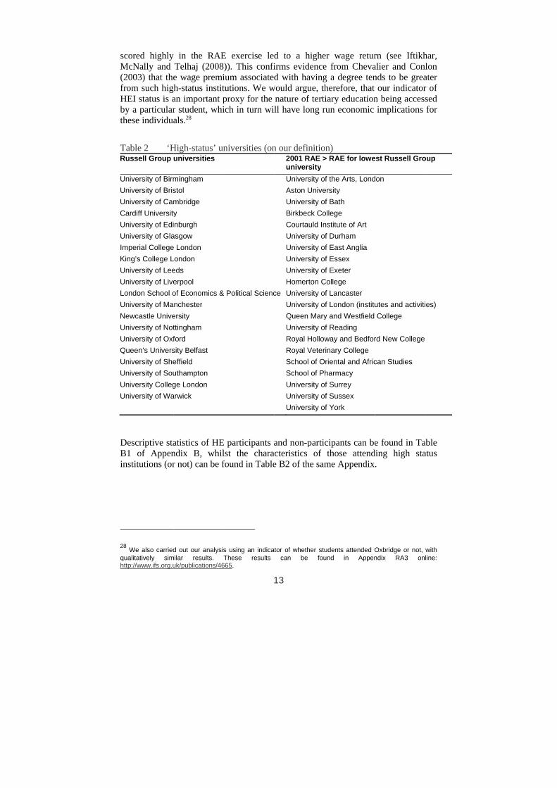
To derive our measure of HE status, we linked in institution-level average Research Assessment Exercise (RAE) scores from the 2001 exercise, and included all Russell Group institutions, plus any UK university with an average 2001 RAE rating exceeding the lowest average RAE score found among the Russell Group universities. This gives a total of 41 ‘high-status’ universities (listed in Table 2). Using this definition, 35% of HE participants attend a ‘high-status’ university in their first year, which equates to 11% of our sample as a whole (including participants and non-participants).

We recognise that such definitions of institution status are, by their very nature, somewhat arbitrary. In particular, different academic departments within HEIs will be of differing qualities and we ignore such subject differences here (although recent evidence (Chevalier, 2009) suggests that institutional quality matters more than departmental quality for future wages). Additionally, we have defined status according to research quality and membership of the Russell Group. These indicators of status are not necessarily important in determining the quality of undergraduates’ university experience. For example, students might focus more on teaching contact time or expenditure per pupil. However, recent evidence suggests that obtaining a degree from a Russell Group institution and attending an HEI that

25 Private school students (and others for whom these characteristics are missing for some reason) are included by using missing dummies where necessary. 26 Of course, we do not have public examination results at age 18 for all pupils, as some will have chosen not to stay on in education beyond age 16. For these individuals, we include a missing results dummy. 27 In our analysis of the type of HE institution attended (for HE participants only), we also make use of the pupil’s tariff score (the record of their qualifications available to the university at the time of application).

sM(fHbth

TR

UUUCUUImKUULUNUUQUUUU

DBin

2

qh

scored highly McNally and 2003) that the

from such higHEI status is aby a particularhese individua

Table 2 ‘HRussell Group

University of BirmUniversity of BrisUniversity of CamCardiff UniversityUniversity of EdiUniversity of Glamperial College

King’s College LUniversity of LeeUniversity of LiveLondon School oUniversity of MaNewcastle UniveUniversity of NotUniversity of OxfQueen’s UniversUniversity of SheUniversity of SouUniversity CollegUniversity of Wa

Descriptive staB1 of Appennstitutions (or

8 We also carriedqualitatively simhttp://www.ifs.org.u

y in the RAETelhaj (2008e wage premih-status institan important pr student, whials.28

High-status’ ununiversities

mingham stol mbridge y nburgh

asgow e London London eds erpool of Economics &nchester

ersity ttingham ford sity Belfast effield uthampton ge London arwick

atistics of HEndix B, whilr not) can be f

d out our analysismilar results. Tuk/publications/46

E exercise led)). This confiium associatedtutions. We wproxy for the ich in turn wil

niversities (on

Political Scienc

E participants alst the charafound in Table

s using an indicaThese results

665.

13

d to a higheirms evidenced with having

would argue, thnature of tertill have long r

n our definitio2001 RAE >universityUniversity oAston UniveUniversity oBirkbeck CoCourtauld InUniversity oUniversity oUniversity oUniversity oHomerton C

ce University oUniversity oQueen MaryUniversity oRoyal HollowRoyal VeterSchool of OSchool of PUniversity oUniversity oUniversity o

and non-particcteristics of e B2 of the sam

tor of whether stucan be fou

er wage reture from Chevag a degree tenherefore, that iary educationrun economic

on) > RAE for lowe

of the Arts, Londersity of Bath ollege nstitute of Art of Durham of East Anglia of Essex of Exeter College of Lancaster of London (instituy and Westfield

of Reading way and Bedforrinary College

Oriental and Africharmacy

of Surrey of Sussex of York

cipants can bethose attend

me Appendix

udents attended Ound in Appen

rn (see Iftikhalier and Connds to be grea

our indicatorn being accessimplications

est Russell Gro

don

utes and activitiCollege

rd New College

can Studies

e found in Tading high sta.

Oxbridge or not, ndix RA3 on

har, lon ater r of sed for

oup

es)

able atus

with line:

14

6. Results 6.1 Participation in Higher Education

In this section, we document the association between socio-economic status (SES) and the likelihood of participating in higher education (HE) at age 19 or 20, and show how this relationship changes once we take into account a range of other individual and school characteristics, plus detailed measures of prior attainment. Due to the well-established differences in educational attainment by gender, we do this separately for males and females (in Tables 3 and 4 respectively).29

The first column of each table shows the raw differences in HE participation rates by socio-economic quintile. The second column adds controls for individual characteristics and school fixed effects. The remaining columns show how the impact of socio-economic status is mediated by the successive inclusion of measures of prior attainment at ages 11, 14, 16 and 18. The first columns show that there is a large and significant raw socio-economic gradient in HE participation rates: for example, being in the bottom SES quintile (compared with the top SES quintile) reduces the likelihood of going to university at age 19 or 20 by 40.7 percentage points for boys and 44.6 percentage points for girls. Similarly, males (females) in the middle SES quintile are 25.3 (25.1) percentage points less likely to participate in HE at age 19/20 than students in the top SES quintile. Once we take into account a variety of individual characteristics and school fixed effects, these gaps fall by around 30% for boys and 20% for girls (Column 2), suggesting that differences in individual characteristics and the types of schools attended by young people from different socio-economic backgrounds provide some explanation for why young people from poorer families are less likely to go to university than young people from richer families. Columns 3 through 6 show how university participation rates vary between students from different socio-economic backgrounds, but who otherwise have similar observable characteristics, attend the same schools, and follow the same pattern of attainment from age 11 to age 18.

As might be expected, the inclusion of controls for prior educational attainment reduces the effect of socio-economic status on HE participation rates. For example, the impact (on the likelihood of going to university at age 19 or 20) of being in the bottom SES quintile (compared to the top SES quintile) falls from 29.2 to 21.1 percentage points for boys – and from 35.8 to 25.6 percentage points for girls – once we add in age 11 test results. Similarly, the effect of being in the middle SES quintile (compared to the top SES quintile) falls from 18.0 to 13.8 percentage points for boys, and from 20.2 to 15.3 percentage points for girls. This suggests that socio-economic disadvantage has already had an impact on academic outcomes at the age

29 Full details of all coefficients can be found in Appendix RA4 online: http://www.ifs.org.uk/publications/4665.

15

of 11 and that this disadvantage explains a significant proportion of the gap in HE participation at age 19 or 20.30

Table 3 Gradients in HE participation for state and private school males No

controls Individual

and school

controls

Plus age 11 test results


Plus age 16 exam results


2nd SES quintile -0.161** -0.108** -0.085** -0.069** -0.047** -0.024** [0.004] [0.003] [0.002] [0.002] [0.002] [0.002] Middle SES quintile -0.253** -0.180** -0.138** -0.107** -0.068** -0.033** [0.005] [0.003] [0.003] [0.002] [0.002] [0.002] 4th SES quintile -0.342** -0.250** -0.186** -0.142** -0.084** -0.038** [0.005] [0.003] [0.003] [0.002] [0.002] [0.002] Bottom SES quintile -0.407** -0.292** -0.211** -0.156** -0.087** -0.041** [0.005] [0.003] [0.003] [0.003] [0.002] [0.002] Observations 590,964 590,964 590,964 590,964 590,964 590,964 R-squared 0.100 0.104 0.252 0.287 0.422 0.581 No. of clusters 4,363 4,363 4,363 4,363 4,363 F-test of additional controls (p-value)

0.000 0.000 0.000 0.000 0.000

Notes: all specifications include a cohort dummy. This cohort effect is small (less than 1 percentage point) but significant in the final specification. Standard errors clustered at school level and reported in square brackets. ** indicates significance at the 1% level and * at the 5% level.

Table 4 Gradients in HE participation for state and private school females No

controls Individual

and school

controls





2nd SES quintile -0.142** -0.110** -0.085** -0.068** -0.047** -0.024** [0.004] [0.003] [0.002] [0.002] [0.002] [0.002]

Middle SES quintile -0.251** -0.202** -0.153** -0.121** -0.080** -0.038** [0.005] [0.003] [0.003] [0.002] [0.002] [0.002]

4th SES quintile -0.362** -0.294** -0.217** -0.168** -0.104** -0.048** [0.005] [0.003] [0.003] [0.003] [0.002] [0.002]

Bottom SES quintile -0.446** -0.358** -0.256** -0.193** -0.113** -0.053** [0.005] [0.003] [0.003] [0.003] [0.002] [0.002]

Observations 572,881 572,881 572,881 572,881 572,881 572,881 R-squared 0.108 0.075 0.21 0.277 0.424 0.574 No. of clusters 4,414 4,414 4,414 4,414 4,414 F-test of additional controls (p-value)

0.000 0.000 0.000 0.000 0.000

30 Unfortunately, our data do not contain earlier test results, making it impossible to assess when these differences in attainment (by socio-economic status) first emerge for our cohorts. However, it is worth noting that much of the recent literature suggests that it is likely to have been significantly earlier than age 11 (see, for example, Cunha and Heckman (2007)).

16

Notes: see notes to Table 3.

The explanatory power of prior attainment also appears to increase with age: that is to say, the coefficients on our SES quintiles are reduced by more as a result of the inclusion of later test results than they are as a result of the inclusion of earlier test scores. For example, while the coefficients on socio-economic status are reduced by around 20% for both boys and girls following the inclusion of age 14 results, they are reduced by between 30% and 40% when we add age 16 GCSE results. This suggests that an important part of the HE participation story is what happens to the academic trajectories of the most disadvantaged students between the ages of 11 and 16 (and consequently whether they choose to stay on beyond compulsory schooling) (see Chowdry et al., 2008, for further details). Once we have added in all available measures of prior attainment (i.e. up to age 18), the association between socio-economic status and HE participation rates is substantially reduced. In particular, boys (girls) in the bottom SES quintile are now 4.1 (5.3) percentage points less likely to go to university at age 19 or 20 than boys (girls) in the top SES quintile; this is around 10% (12%) of the raw differences of 40.7 (44.6) percentage points respectively. Similarly, boys (girls) from the middle SES quintile are 3.3 (3.8) percentage points less likely to go to university than boys (girls) from the top SES quintile, a reduction of 87% (85%) compared to the raw differences of 25.3 (25.1) percentage points. It is interesting to note that the socio-economic gradient in university attendance, including all available measures of prior attainment, suggests a relatively large difference in participation rates between the top and second SES quintiles (of 2.4 percentage points for girls and boys), and a roughly equivalent gap between the second and bottom SES quintiles (of 2.7 percentage points for girls and 1.7 percentage points for boys). This suggests that much of the socio-economic gap in HE participation rates is being driven by particularly high participation rates for individuals at the top of the income distribution. Interestingly, this pattern persists if we exclude private school students from our analysis31, suggesting that the high participation rates amongst the very rich are not entirely driven by the ability of private schools to get their students into university. Of course, we acknowledge that after age 16 students may only choose to stay on in school and take A-levels if they intend to go to university. If they feel that university is not for them, they may not take A-levels, or if they do, they may not put in much effort if their grades are not so important to them, as compared to students going on to university. Furthermore, university places are often awarded on the basis of predicted A-level grades. The age 18 test scores that we use in our final specification may therefore be endogenous. By contrast, at age 16, all pupils have to remain in full time education and GCSEs have currency even for those intending to leave the education system. The specification that controls for age 16 public

31 See Appendix RA2 online: http://www.ifs.org.uk/publications/4665.

17

examination test scores indicates that students from the top SES quintile are between 9 and 11 percentage points more likely to participate in HE than students with similar GCSE grades from the bottom SES quintile, and between 7 and 8 percentage points more likely to attend than students with similar GCSE grades from the middle SES quintile. These figures still represent substantial reductions in the socio-economic gradient in university participation compared to the sizeable raw gaps described above. Another potential source of endogeneity, even for our penultimate specification, is pupils’ choice of school. To investigate the extent to which the inclusion of school fixed effects may be driving our results, we also estimate a model without these effects (see Appendix C for details). These results suggest that in models that control fully for individual characteristics and prior attainment, school fixed effects do not make a significant difference to the estimates of the socio-economic gap in HE participation. This suggests that the non-random selection of pupils into schools is not biasing our results. In summary, our analysis shows that the raw differences in university participation rates between advantaged and disadvantaged students are extremely large. However, once we take into account students’ prior attainment (particularly at ages 16 and 18), these substantial gaps in participation are markedly reduced. This suggests that one of the main challenges to widening participation for pupils from poorer socio-economic backgrounds is to increase the proportion of pupils getting good GCSE and A-level results.

6.2 Status of HE Institution Attended

In this section, we move on to document the relationship between socio-economic status (SES) and the likelihood of attending a high status institution at age 19 or 20, conditional on participating, and show how this relationship changes once we take into account individual and school characteristics, plus prior attainment. It is worth noting that our data comes from a period during which fees were generally undifferentiated across subjects and institutions. Tables 5 and 6 present our results for boys and girls respectively.32 Column 1 of Table 5 (6) presents raw estimates of the impact of socio-economic status on the likelihood of attending a high-status institution for boys (girls) who participate in higher education at age 19 or 20. These raw figures show that there are large socio-economic differences in the probability of attending a high-status university. For example, males (females) in the bottom SES quintile are 31.7 (32.4) percentage points less likely to attend a high-status university than males (females) in the top SES quintile (conditional on participating). Similarly, males (females) from the middle SES quintile are 22.5 (23.1) percentage points less likely to attend a high status institution than males (females) from the top SES quintile.

32 Full details of all coefficients can be found in Appendix RA4 online: http://www.ifs.org.uk/publications/4665.

18

Table 5 Gradients in probability of attending a ‘high-status’ HEI amongst male participants from state and private schools

No controls

Individual and

school controls





2nd SES quintile -0.154** -0.044** -0.039** -0.034** -0.027** -0.016** [0.008] [0.004] [0.003] [0.003] [0.003] [0.003]


4th SES quintile -0.274** -0.108** -0.087** -0.070** -0.046** -0.023** [0.009] [0.005] [0.004] [0.004] [0.004] [0.004]



0.000 0.000 0.000 0.000 0.000

Notes: HE participants only. All specifications include cohort dummy. This cohort effect is small (less than 1 percentage point) but significant in the final specification. Standard errors clustered at school level and reported in square brackets. ** indicates significance at the 1% level, * at the 5% level.

Table 6 Gradients in probability of attending a ‘high-status’ HEI amongst female participants from state and private schools

No controls

Individual and

school controls





2nd SES quintile -0.161** -0.051** -0.043** -0.038** -0.034** -0.022** [0.006] [0.003] [0.003] [0.003] [0.003] [0.003]


4th SES quintile -0.291** -0.129** -0.104** -0.088** -0.070** -0.043** [0.007] [0.004] [0.004] [0.004] [0.004] [0.003]



0.000 0.000 0.000 0.000 0.000

Notes: see notes to Table 5.

Interestingly, the inclusion of individual characteristics and school fixed effects (Column 2) reduces the impact of socio-economic status on attendance at a high-status HEI by more than it reduces the impact of socio-economic status on HE

19

participation (in Tables 3 and 4 above): the attendance gap between participants from the top and bottom SES quintiles is reduced by around 50-70% for boys and girls (compared with a reduction of around 20-30% for HE participation). This is an interesting result, to which we return later. Thereafter, the inclusion of each of our measures of prior attainment makes a relatively smaller difference to the coefficients on socio-economic status. Nonetheless, once we have added in prior attainment at ages 11, 14, 16 and 18, we find that socio-economic background has a substantially reduced impact on the probability that HE participants will attend high-status institutions. For example, boys (girls) from the bottom SES quintile are now only 2.5 (4.3) percentage points less likely to attend a high status institution (conditional on participation) than boys (girls) from the top SES quintile; this is just 8% (13%) of the raw gaps of 31.7 (32.4) percentage points respectively. Similarly, boys (girls) from the middle SES quintile are only 2.6 (3.2) percentage points less likely to attend a high status institution than boys (girls) from the top SES quintile, a reduction of 88% (86%) compared to the raw gaps of 22.5 (23.1) percentage points.

Given our finding that the addition of individual and school characteristics reduced the socio-economic gap in HE participation at a high status institution by more than it reduced the gap in HE participation overall, we investigated the role of schools in explaining participation in a high quality institution in more detail, by running models excluding school fixed effects (see Appendix C). In contrast to our findings for participation overall (discussed above), excluding school fixed effects from our model of participation at a high status institution significantly increased the socio-economic gap in our final specification, from 2.5 (4.3) to 3.7 (6.0) percentage points for males (females), an increase of around 40 per cent for both boys and girls. This suggests that schools may have an important role to play in encouraging students from poorer families to apply to high status universities. As we saw with our overall participation results, there is also a similar difference between the proportions of individuals who attend high status institutions from the top and second SES quintiles (1.6 percentage points for boys and 2.2 percentage points for girls) and the second and bottom SES quintiles (0.9 percentage points for boys and 2.1 percentage points for girls). Again, these results hold even if we exclude private school students from our analysis33, suggesting that the socio-economic gap in high status participation is not driven solely by particularly high attendance amongst private school students. In summary, we find very large raw socio-economic differences in the likelihood of attending a high status university (conditional on participation). However, once we control for a range of individual characteristics and school fixed effects, plus detailed measures of prior attainment, these differences are substantially reduced. These findings again highlight the importance of increasing attainment amongst

33 See Appendix RA2 online: http://www.ifs.org.uk/publications/4665.

20

poorer children in secondary schools as a route through which the socio-economic gap in HE participation (including at a high status university) might be reduced.

7. Conclusions

This paper has shown that students from poorer backgrounds are much less likely to participate in tertiary education than students from richer backgrounds. However, our findings suggest that this socio-economic gap in university participation does not emerge at the point of entry into higher education. In other words, the socio-economic gap in HE participation does not arise simply because poorer students face the same choices at 18 but choose not to go to university. Instead, it comes about largely because poorer pupils do not achieve as highly in secondary school as their more advantaged counterparts, confirming the general trend in the literature that socio-economic gaps emerge relatively early in individuals’ lives. It is important to note that a socio-economic gap in participation does remain on entry into university, even after allowing for prior attainment, but it is modest relative to the magnitude of the raw differences once we control for A level achievement, and to a lesser extent GCSE scores. The implication is that focusing policy interventions on encouraging disadvantaged pupils at age 18 to apply to university is unlikely to have a major impact on reducing the raw socio-economic gap in university participation. These results also potentially explain why the introduction of tuition fees did not have a major negative impact on widening participation, though of course we cannot rule out the possibility that further large increases in tuition fees may widen the socio-economic gap. Our results controlling for age 16 attainment suggest that there may be some gain from targeting poorer pupils with good GCSE results, but again, this relatively later intervention is unlikely to have a large effect on widening participation as compared to intervention at, say, age 11. That is not to say that universities should stop their outreach work to disadvantaged students who continue into post-compulsory education, but simply that such activities are unlikely to tackle the more major problem underlying the socio-economic gap in university participation – namely, the underachievement of disadvantaged pupils in secondary school. We argue that policy-makers should be focusing more on improving the educational performance of disadvantaged children in secondary school as a way of enabling them to access higher education. Yet clearly we need to be cautious about this conclusion. First, students look forward when making decisions about what qualifications to attempt at ages 16 and 18, and indeed when deciding how much effort to put into school work. If disadvantaged pupils feel that HE is ‘not for people like them’, then it may be that their achievement in school simply reflects anticipated barriers to participation in tertiary education, rather than the other way around. This suggests that outreach activities will still be required to raise students’ aspirations about university, but that they might perhaps be better targeted on

21

younger children in secondary school (as indeed is happening with AimHigher and other widening participation interventions).34 Another issue is that we know children’s non-cognitive skills are also important, i.e. they influence individuals’ life time outcomes, and appear more malleable later in childhood (Carneiro and Heckman, 2003). Unfortunately, we are not able to measure students’ non-cognitive skills in our data. It is possible that, although we find that prior achievement is the biggest driver of HE participation, this could reflect the fact that there is a positive relationship between cognitive and non-cognitive skills. If we had separate controls for cognitive and non-cognitive skill, we might find that it is really pupils’ non-cognitive skills that are the key determinant of their likelihood of going to university. Another aspect of the widening participation agenda that we have explored in this paper surrounds the type of tertiary education experienced by the student. We find that there are large socio-economic gaps in the likelihood of attending a high-status institution (as measured by research intensiveness). Whilst it may well be that research quality is not a good indicator of the overall quality of a university, the additional value of degrees from such institutions means that access to these high status universities is as much an issue as access to the sector as a whole. Again, however, we find that the impact of socio-economic status on the likelihood of attending a high-status university becomes much smaller once we take account of individual characteristics and school fixed effects, plus detailed measures of prior attainment. These results highlight not only the importance of attainment in secondary schools, but also the potentially important role schools seem to be playing in encouraging students from poorer backgrounds to apply to high status institutions.

34 It should be noted, however, that a higher proportion of pupils in the Longitudinal Study of Young People in England report (at age 14) that they are likely to apply to university than are likely to ultimately do so, including those from poorer backgrounds (see Chowdry, Crawford & Goodman, 2009).

References

Bekhradnia, B. (2003), Widening Participation and Fair Access: An Overview of the Evidence, Report from the Higher Education Policy Institute.

Belley, P. and Lochner, L. (2007), ‘The changing role of family income and ability in determining educational achievement’, Journal of Human Capital, vol. 1, pp. 37–89.

Blanden, J. and Gregg, P. (2004), ‘Family income and educational attainment: a review of approaches and evidence for Britain’, Oxford Review of Economic Policy, vol. 20, pp. 245–63.

Blanden, J. and Machin, S. (2004), ‘Educational inequality and the expansion of UK higher education’, Scottish Journal of Political Economy, Special Issue on the Economics of Education, vol. 51, pp. 230–49.

Burke, P. (2004), ‘Women accessing education: subjectivity, policy and participation’, Journal of Access Policy and Practice, vol. 1, pp. 100–18.

Callender, C. (2003), ‘Student financial support in higher education: access and exclusion’, in M. Tight (ed.), Access and Exclusion: International Perspectives on Higher Education Research, London: Elsevier Science.

Carneiro, P. and Heckman, J. (2002), ‘The evidence on credit constraints in post-secondary schooling’, Economic Journal, vol. 112, pp. 705–34.

Carneiro, P. and Heckman, J. (2003), ‘Human capital policy’, in J. Heckman, A. Krueger and B. Friedman (eds), Inequality in America: What Role for Human Capital Policies?, Cambridge, MA: MIT Press.

Chevalier, A. (2009), Does higher education quality matter in the UK?, Royal Holloway, University of London, mimeo

Chevalier, A. and Conlon, G. (2003), ‘Does it pay to attend a prestigious university?’, Centre for the Economics of Education (CEE), Discussion Paper no. 33.

Chowdry, H., Crawford, C., Dearden, L., Goodman, A. and Vignoles, A. (2008), ‘Understanding the determinants of participation in higher education and the quality of institute attended: analysis using administrative data’, Institute for Fiscal Studies, mimeo.

Chowdry, H., Crawford, C. and Goodman, A. (2009), ‘Drivers and Barriers to Educational Success: Evidence from the Longitudinal Study of Young People in England’, DCSF Research Report RR102.

CMPO (2006), Family Background and Child Development up to Age 7 in the Avon Longitudinal Survey of Parents and Children (ALSPAC), DfES Research Report no. RR808A.

Connor, H., Burton, R., Pearson, R., Pollard, E. and Regan, J. (1999), Making the Right Choice: How Students Choose University and Colleges, London: Institute for Employment Studies (IES).

Connor, H. and Dewson, S. with C. Tyers, J. Eccles, J. Regan and J. Aston (2001), Social Class and Higher Education: Issues Affecting Decisions on Participation by Lower Social Class Groups, DfES Research Report no. 267.

Connor, H., Tyers, C., Modood, R. and Hillage, J. (2004), Why the Difference? A Closer Look at Higher Education Minority Ethnic Students and Graduates, DfES Research Report no. 552.

23

Crawford, C. and Dearden, L. (2010), ‘The impact of the 2006-07 HE finance reforms on HE participation’, Report to the Department of Business, Innovation and Skills, mimeo.

Cunha, F. and Heckman, J. (2007), ‘The technology of skill formation’, American Economic Review, vol. 92, pp. 31–47.

Cunha, F., Heckman, J., Lochner, L. and Masterov, D. (2006), ‘Interpreting the evidence on life cycle skill formation’, in E. Hanushek and F. Welch (eds), Handbook of the Economics of Education, Amsterdam: North-Holland.

Dearden, L., McGranahan, L. and Sianesi, S. (2004), ‘The role of credit constraints in educational choices: evidence from the NCDS and BCS70’, CEE Discussion Paper No. 48, London.

Dearden, L., Fitzsimons, E. and Wyness, G. (2010), ‘Estimating the Impact of Up-front Fees and Student Support on University Participation’, Report to the Department of Business, Innovation and Skills, mimeo.

Dearing, R. (1997), Higher Education in the Learning Society, Report of the National Committee of Inquiry into Higher Education, Norwich: HMSO.

Demack, S., Drew, D. and Grimsley, M. (2000), ‘Minding the gap: ethnic, gender and social class differences in attainment at 16, 1988–95’, Race, Ethnicity and Education, vol. 3, pp. 112–41.

Department for Education and Skills (2003), Widening Participation in Higher Education, London: DfES (http://www.dfes.gov.uk/hegateway/uploads/EWParticipation.pdf).

Department for Education and Skills (2006), Widening Participation in Higher Education, London: DfES (http://www.dcsf.gov.uk/hegateway/uploads/6820-DfES-WideningParticipation2.pdf).

Feinstein, L. (2003), ‘Inequality in the early cognitive development of British children in the 1970 cohort’, Economica, vol. 70, pp. 73–98.

Fielding (2004) The Role of the Hausman Test and whether Higher Level Effects should be treated as Random or Fixed, Multilevel Modelling Newsletter, vol. 16, no,2.

Finegold, D. (2006), ‘The roles of higher education in a knowledge economy’, Rutgers University, mimeo.

Forsyth, A. and Furlong, A. (2003), ‘Access to higher education and disadvantaged young people’, British Educational Research Journal, vol. 29, pp. 205–25.

Galindo-Rueda, F., Marcenaro-Gutierrez, O. and Vignoles, A. (2004), ‘The widening socio-economic gap in UK higher education’, National Institute Economic Review, no. 190, pp. 70–82.

Gayle, V., Berridge, D. and Davies, R. (2002), ‘Young people’s entry into higher education: quantifying influential factors’, Oxford Review of Education, vol. 28, pp. 5–20.

Glennerster, H. (2001), ‘United Kingdom education 1997–2001’, Centre for the Analysis of Social Exclusion (CASE), Working Paper no. 50.

Gorard, S. (2000), Education and Social Justice: The Changing Composition of Schools and Its Implications, Cardiff: University of Wales Press.

Gorard, S., Smith, E., May, H., Thomas, L., Adnett, N. and Slack, K. (2006), Review of Widening Participation Research: Addressing the Barriers to Widening Participation in Higher Education, Report to HEFCE by the

24

University of York, Higher Education Academy and Institute for Access Studies, Bristol: HEFCE.

Haggis, T. and Pouget, M. (2002), ‘Trying to be motivated: perspectives on learning from younger students accessing higher education’, Teaching in Higher Education, vol. 7, pp. 323–36.

Haveman, R. and Wolfe, B. (1995), ‘The determinants of children’s attainments: a review of methods and findings’, Journal of Economic Literature, vol. 33, pp. 1829–78.

Heenan, D. (2002), ‘Women, access and progression: an examination of women’s reasons for not continuing in higher education following the completion of the Certificate in Women’s Studies’, Studies in Continuing Education, vol. 24, pp. 40–55.

Hobbs, G. and Vignoles, A. (2007) ‘Is Free School Meal Status a Valid Proxy for Socio-Economic Status (in Schools Research)?’, Centre for the Economics of Education Discussion Paper CEEDP0084, London School of Economics.

Iftikhar, H., McNally, S. and Telhaj, S. (2008), ‘University quality and graduate wages in the UK’, Centre for Economics of Education, mimeo; output from ESRC-TLRP project ‘Widening Participation in Higher Education: A Quantitative Analysis’.

Jenkins, A., Vignoles, A., Wolf, A. and Galindo-Rueda, F. (2003) ‘The determinants and labour market effects of lifelong learning’, Applied Economics, Vol.35, No.16, pp.1711-1721.

Machin, S. and Vignoles, A. (2004), ‘Educational inequality: the widening socio-economic gap’, Fiscal Studies, vol. 25, pp. 107–28.

Meghir, C. and Palme, M. (2005), ‘Educational reform, ability, and family background’, American Economic Review, vol. 95, pp. 414–24.

Osborne, M., Marks, A. and Turner, E. (2004), ‘Becoming a mature student: how adult applicants weigh the advantages and disadvantages of higher education’, Higher Education: The International Journal of Higher Education and Educational Planning, vol. 48, pp. 291–315.

Pennell, H. and West, A. (2005), ‘The impact of increased fees on participation in higher education in England’, Higher Education Quarterly, vol. 59, pp. 127–37.

Powdthavee, N. and Vignoles, A. (2009), ‘The Socioeconomic Gap in University Dropouts’, The B.E. Journal of Economic Analysis & Policy, vol. 9, issue 1, article 19, available at: http://www.bepress.com/bejeap/vol9/iss1/art19.

Quinn, J. (2004), ‘Understanding working-class “drop-out” from higher education through a socio-cultural lens: cultural narratives and local contexts’, International Studies in Sociology of Education, vol. 14, pp. 57–74.

Raffe, D., Croxford, L., Iannelli, C., Shapira, M. and Howieson, C. (2006), Social-Class Inequalities in Education in England and Scotland, Special CES Briefing no. 40, Edinburgh: Centre for Educational Sociology.

Reay, D. (2003), ‘A risky business? Mature working-class women students and access to higher education’, Gender and Education, vol. 15, pp. 301–17.

Rutter, M., Moffitt, E. and Caspi, A. (2006), ‘Gene–environment interplay and psychopathology: multiple varieties but real effects’, Journal of Child Psychology and Psychiatry, vol. 47, pp. 226–61.

25

Sammons, P. (1995), ‘Gender, ethnic and socio-economic differences in attainment and progress: a longitudinal analysis of student achievement over 9 years’, British Educational Research Journal, vol. 21, pp. 465–85.

Strand, S. (1999), ‘Ethnic group, sex and economic disadvantage: associations with pupil’s educational progress from Baseline to the end of Key Stage 1’, British Educational Research Journal, vol. 25, pp. 179–202.

Universities UK (2007), Variable Tuition Fees in England: Assessing their Impact on Students and Higher Education Institutions, London: UUK.

Wyness, G. (2009), The impact of higher education finance in the UK, PhD thesis, Institute of Education, University of London.

26

Appendix A Table A1 Characteristics of LSYPE cohort members by socio-economic quintile

Bottom SES

quintile

2 Middle SES

quintile

4 Top SES quintile

Household income (average W1 to W3)

£11,206 £13,946 £17,454 £21,591 £27,645

Mum has a degree 8% 13% 20% 30% 40% Dad has higher managerial/professional occupation

11% 20% 29% 43% 60%

Family in financial difficulties

15% 10% 7% 5% 3%

Family living in socially rented housing

63% 33% 18% 9% 3%

Notes: we constructed our socio-economic quintiles (on the basis of individual FSM eligibility and other neighbourhood-based measures of socio-economic status) for LSYPE cohort members, and then summarised the characteristics of individuals in each of these quintiles. Characteristics are reported in Wave 1, at age 14, unless otherwise specified.

27

Appendix B Table B1 Personal characteristics of HE participants and non-participants Characteristic HE

participants HE non-

participants Difference

Achieved 5 A*–C GCSE grades 0.838 0.257 0.581** Reached Level 3 threshold by 18 via any route 0.885 0.161 0.725** Male 0.448 0.536 -0.088** Top SES quintile 0.334 0.124 0.210** 2nd SES quintile 0.258 0.177 0.081** Middle SES quintile 0.194 0.207 -0.013** 4th SES quintile 0.131 0.236 -0.105** Bottom SES quintile 0.083 0.257 -0.174** Attended private school at age 16 0.122 0.045 0.077** Observations 370,021 793,824 Notes: The numbers presented in each column are the mean values of each characteristic for HE participants at age 19 or 20 (column 1) and non-participants (column 2), and the difference between these means (column 3). For all those characteristics taking values either 0 or 1, the mean values in columns 1 and 2 are interpretable as the proportion of participants or non-participants who take the value 1 for that characteristic. ** indicates significance at the 1% level and * at the 5% level.

Table B2 Personal characteristics of HE participants who attend a high-status institution and HE participants who do not Characteristic Attend a

high-status institution

In HE but do not

attend a high-status institution

Difference

Achieved 5 A*–C GCSE grades 0.959 0.773 0.185** Reached Level 3 threshold by 18 via any route 0.967 0.841 0.126** Male 0.457 0.443 0.014** Top SES quintile 0.476 0.257 0.218** 2nd SES quintile 0.251 0.262 -0.010** Middle SES quintile 0.15 0.218 -0.068** 4th SES quintile 0.08 0.158 -0.077** Bottom SES quintile 0.042 0.105 -0.063** Attended private school at age 16 0.221 0.069 0.152** Observations 129,560 240,461 Notes: The numbers presented in each column are the mean values of each characteristic for HE participants who attend a high-status institution (column 1) and HE participants who do not attend a high-status institution (column 2), and the difference between these means (column 3). For all those characteristics taking values either 0 or 1, the mean values in columns 1 and 2 are interpretable as the proportion of HE participants at high-status (respectively other) institutions who take the value 1 for that characteristic. ** indicates significance at the 1% level and * at the 5% level.

28

Appendix C Table C1 Gradients in HE participation for state and private school males (without school fixed effects)

No controls

Individual controls

only

Plus Key Stage 2 results




2nd SES quintile -0.161** -0.150** -0.108** -0.084** -0.060** -0.028** [0.004] [0.004] [0.003] [0.002] [0.002] [0.002] Middle SES quintile -0.253** -0.248** -0.173** -0.128** -0.084** -0.036** [0.005] [0.004] [0.003] [0.003] [0.002] [0.002] 4th SES quintile -0.342** -0.336** -0.230** -0.167** -0.101** -0.041** [0.005] [0.005] [0.003] [0.003] [0.002] [0.002] Bottom SES quintile -0.407** -0.393** -0.263** -0.184** -0.106** -0.043** [0.005] [0.005] [0.003] [0.003] [0.002] [0.002] Observations 590,964 590,964 590,964 590,964 590,964 590,964 R-squared 0.100 0.150 0.268 0.330 0.425 0.582 F-test of additional controls (p-value)

0.000 0.000 0.000 0.000 0.000

Notes: all specifications include a cohort dummy. Standard errors clustered at school level and reported in square brackets. ** indicates significance at the 1% level and * at the 5% level.

Table C2 Gradients in HE participation for state and private school females (without school fixed effects)

No controls

Individual controls

only





2nd SES quintile -0.142** -0.149** -0.106** -0.082** -0.059** -0.027** [0.004] [0.004] [0.003] [0.003] [0.002] [0.002]


4th SES quintile -0.362** -0.379** -0.260** -0.190** -0.117** -0.048** [0.005] [0.005] [0.003] [0.003] [0.003] [0.002]

Top SES quintile -0.446** -0.459** -0.306** -0.216** -0.126** -0.049** [0.005] [0.005] [0.004] [0.003] [0.003] [0.002]

Observations 572,881 572,881 572,881 572,881 572,881 572,881 R-squared 0.108 0.154 0.273 0.333 0.425 0.576 F-test of additional controls (p-value)

0.000 0.000 0.000 0.000 0.000

Notes: see notes to Table C1.

29

Table C3 Gradients in probability of attending a ‘high-status’ HEI amongst male participants from state and private schools (without school fixed effects)

No controls

Individual controls

only





2nd SES quintile -0.154** -0.074** -0.057** -0.049** -0.040** -0.023** [0.008] [0.005] [0.004] [0.004] [0.003] [0.003] Middle SES quintile -0.225** -0.142** -0.108** -0.088** -0.066** -0.036** [0.008] [0.006] [0.005] [0.004] [0.004] [0.003] 4th SES quintile -0.274** -0.186** -0.138** -0.108** -0.075** -0.039** [0.009] [0.007] [0.006] [0.005] [0.004] [0.004] Bottom SES quintile -0.317** -0.224** -0.158** -0.116** -0.075** -0.037** [0.009] [0.008] [0.007] [0.006] [0.005] [0.004] Observations 165,634 165,634 165,634 165,634 165,634 165,634 R-squared 0.056 0.078 0.170 0.215 0.307 0.461 F-test of additional controls (p-value)

0.000 0.000 0.000 0.000 0.000


Table C4 Gradients in probability of attending a ‘high-status’ HEI amongst female participants from state and private schools (without school fixed effects)

No controls

Individual controls

only





2nd SES quintile -0.161** -0.086** -0.067** -0.058** -0.051** -0.033** [0.006] [0.005] [0.004] [0.004] [0.003] [0.003]


4th SES quintile -0.291** -0.215** -0.164** -0.134** -0.106** -0.067** [0.007] [0.006] [0.005] [0.005] [0.004] [0.004]

Top SES quintile -0.324** -0.248** -0.180** -0.138** -0.103** -0.060** [0.007] [0.007] [0.005] [0.005] [0.005] [0.004]

Observations 204,387 204,387 204,387 204,387 204,387 204,387 R-squared 0.061 0.080 0.160 0.197 0.250 0.396 F-test of additional controls (p-value)

0.000 0.000 0.000 0.000 0.000


Documents

Widening Participation in Higher Education