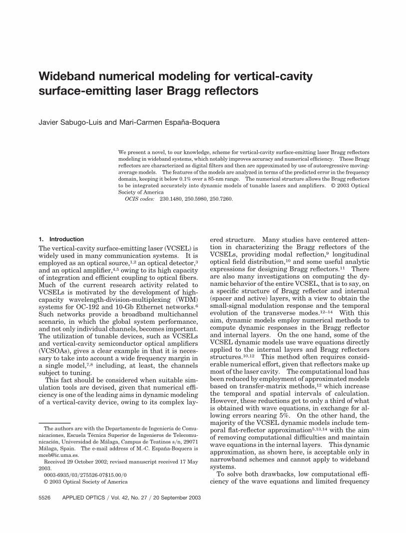
Wideband numerical modeling for vertical-cavitysurface-emitting laser Bragg reflectors

Javier Sabugo-Luis and Mari-Carmen Espana-Boquera

We present a novel, to our knowledge, scheme for vertical-cavity surface-emitting laser Bragg reflectorsmodeling in wideband systems, which notably improves accuracy and numerical efficiency. These Braggreflectors are characterized as digital filters and then are approximated by use of autoregressive moving-average models. The features of the models are analyzed in terms of the predicted error in the frequencydomain, keeping it below 0.1% over a 85-nm range. The numerical structure allows the Bragg reflectorsto be integrated accurately into dynamic models of tunable lasers and amplifiers. © 2003 OpticalSociety of America

OCIS codes: 230.1480, 250.5980, 250.7260.

1. Introduction

The vertical-cavity surface-emitting laser �VCSEL� iswidely used in many communication systems. It isemployed as an optical source,1,2 an optical detector,3and an optical amplifier,4,5 owing to its high capacityof integration and efficient coupling to optical fibers.Much of the current research activity related toVCSELs is motivated by the development of high-capacity wavelength-division-multiplexing �WDM�systems for OC-192 and 10-Gb Ethernet networks.6Such networks provide a broadband multichannelscenario, in which the global system performance,and not only individual channels, becomes important.The utilization of tunable devices, such as VCSELsand vertical-cavity semiconductor optical amplifiers�VCSOAs�, gives a clear example in that it is neces-sary to take into account a wide frequency margin ina single model,7,8 including, at least, the channelssubject to tuning.

This fact should be considered when suitable sim-ulation tools are devised, given that numerical effi-ciency is one of the leading aims in dynamic modelingof a vertical-cavity device, owing to its complex lay-

The authors are with the Departamento de Ingenierıa de Comu-nicaciones, Escuela Tecnica Superior de Ingenieros de Telecomu-nicacion, Universidad de Malaga, Campus de Teatinos s�n, 29071Malaga, Spain. The e-mail address of M.-C. Espana-Boquera ismceb@ic.uma.es.

Received 29 October 2002; revised manuscript received 17 May2003.

0003-6935�03�275526-07$15.00�0© 2003 Optical Society of America

5526 APPLIED OPTICS � Vol. 42, No. 27 � 20 September 2003

ered structure. Many studies have centered atten-tion in characterizing the Bragg reflectors of theVCSELs, providing modal reflection,9 longitudinaloptical field distribution,10 and some useful analyticexpressions for designing Bragg reflectors.11 Thereare also many investigations on computing the dy-namic behavior of the entire VCSEL, that is to say, ona specific structure of Bragg reflector and internal�spacer and active� layers, with a view to obtain thesmall-signal modulation response and the temporalevolution of the transverse modes.12–14 With thisaim, dynamic models employ numerical methods tocompute dynamic responses in the Bragg reflectorand internal layers. On the one hand, some of theVCSEL dynamic models use wave equations directlyapplied to the internal layers and Bragg reflectorsstructures.10,12 This method often requires consid-erable numerical effort, given that reflectors make upmost of the laser cavity. The computational load hasbeen reduced by employment of approximated modelsbased on transfer-matrix methods,12 which increasethe temporal and spatial intervals of calculation.However, these reductions get to only a third of whatis obtained with wave equations, in exchange for al-lowing errors nearing 5%. On the other hand, themajority of the VCSEL dynamic models include tem-poral flat-reflector approximation5,13,14 with the aimof removing computational difficulties and maintainwave equations in the internal layers. This dynamicapproximation, as shown here, is acceptable only innarrowband schemes and cannot apply to widebandsystems.

To solve both drawbacks, low computational effi-ciency of the wave equations and limited frequency

characterization of the temporal flat-reflector approx-imation, we present in this paper a new descriptionmethod of Bragg reflectors in the VCSEL, conceivedto be part of the dynamic models of the VCSEL.This description method is based on autoregressivemoving-average �ARMA� models, mostly used in dig-ital signal processing to approximate generally un-known systems by linear discrete filters with the helpof statistical analysis.15 Although the Bragg reflec-tor is not an unknown system, the ARMA techniquesremain suitable, and their complexity is even lowerbecause there is no need of statistical analysis. Byemploying an ARMA model for the Bragg reflectorresponse, we achieve a full dynamic characterizationin a wide frequency margin, keeping the error in-duced below thresholds as small as 0.01% and 0.1%.The numerical efficiency of the model is nearly 2orders of magnitude better than for a complete wave-equation analysis, and this with just a little numer-ical penalty as compared with the temporal flat-reflector approximation. This scheme can bedirectly integrated into dynamic models of tunableVCSELs or VCSOAs, principally oriented to work inWDM systems located in the 1550-nm minimum-attenuation window and by use of the C �1535–1565-nm� and L �1570–1610-nm� bands.

2. Theoretical Analysis

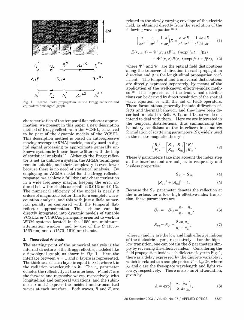
The starting point of the numerical analysis is theinternal structure of the Bragg reflector, modeled likea flow-signal graph, as shown in Fig. 1. Here theinterface between n � 1 and n layers is represented.The thickness of each layer is equal to ��4, where � isthe radiation wavelength in it. The rn parameterdenotes the reflectivity at the interface. F and R arethe forward and regressive waves, respectively, withlongitudinal and temporal variations, and the subin-dexes i and t express the incident and transmittedwaves at each interface. Both waves, R and F, are

related to the slowly varying envelope of the electricfield, as obtained directly from the resolution of thefollowing wave equation16,17:

� �

� z2 ��

�r2 �1r

�

�r�E ��

c2

�2E�t2 �

1c2

��

�t�E�t

, (1)

E�r, z, t� � ���r, z� F� z, t�exp� jt � jz�

� ���r, z� R� z, t�exp� jt � jz�, (2)

where �� and �� are the optical field distributionsalong the transversal direction in each propagationdirection and is the longitudinal propagation coef-ficient. The temporal and transversal distributionsare directly expressed separately, by means of theapplication of the well-known effective-index meth-od.10 The expressions of the transversal distribu-tions can be derived by direct resolution of the spatialwave equation or with the aid of Pade operators.These formulations generally include diffraction ef-fects and thermal behavior, and they have been de-scribed in detail in Refs. 9, 12, and 13, so we do notintend to deal with them. Here we are interested inthe temporal distributions, thus summarizing theboundary conditions at the interfaces in a matrixformulation of scattering parameters �S�, widely usedin the electromagnetic theory18:

�Rt

Ft� � �S11 S12

S21 S22��Fi

Ri� . (3)

These S parameters take into account the index stepat the interface and are subject to reciprocity andlossless properties:

S12 � S21, (4)

�S11�2 � �S22�2 � 1. (5)

Because the S11 parameter denotes the reflection atthe interface, for a low–high effective-index transi-tion, these parameters are

S11 � �S22 �nl � nh

nl � nh, (6)

S12 � S21 �2�nlnh

nl � nh, (7)

where nl and nh are the low and high effective indicesof the dielectric layers, respectively. For the high–low transition, one can obtain the S parameters sim-ply by reversing the effective index. Considering thefield propagation inside each dielectric layer in Fig. 1,there is a delay expressed by the discrete variable z,which is related to a sample period T � �0�2c, where�0 and c are the free-space wavelength and light ve-locity, respectively. There is also an A attenuation,given by

A � exp���s

2�0

4neff� , (8)

Fig. 1. Internal field propagation in the Bragg reflector andequivalent flow-signal graph.

20 September 2003 � Vol. 42, No. 27 � APPLIED OPTICS 5527

where �s is the attenuation coefficient of the dielectriclayer of effective index neff, equal to nl or nh in eachlayer. When the graph is solved, the reflectivity atthe interface can be easily obtained and expressed asa first-order digital filter in the z variable:

rn �S11�1 � A2rn�1S22z

�1� � A2rn�1S12S21z�1

1 � A2rn�1S22z�1 . (9)

Then it becomes clear that when one replaces rn�1with rn in each iteration and starts with rn�1 as themetallization contact reflectivity, the whole reflectiv-ity of Bragg reflectors can be obtained as a digital-filter form, which can be considered an ARMAsystem,15 namely,

r � H� z� � i�0

2N

aiz�i

j�0

2N

bjz�j

, (10)

where r is the whole reflectivity of Bragg reflectorsand ai and bj are the filter coefficients. This digitalfilter contains 2N zeros and 2N poles, where N is thenumber of dielectric pairs of the structure. The Fand R waves making up the solution of the waveequation �2� stand for a modulation of the total elec-tric field, which has a central frequency of � 2���0.Because of that, the reflectivity expressed in Eq. �10�is directly related to the modulated waves. All thesemagnitudes are then treated as low-frequency sig-nals, which correspond to modulations of the opticalcarrier. Their frequencies mean differential fre-quencies, with their reference at the central fre-quency. The reference optical carrier for the VCSELsimulation is placed in 1570 nm, thus including the Land C bands with a modulation margin below 5000GHz. This margin is still small as compared withthe central frequency �191 THz�. For this reason,useful models for VCSELs in WDM systems do notneed to consider the whole digital filter obtained here,which introduces a great computational penalty, butother ARMA schemes can be employed to reduce thecomplexity of the filter. Two different structures areproposed here, separating the poles and the zeros intoan autoregressive �AR� model and a moving-average�MA� model, expressed in Eqs. �11� and �12�, respec-tively,

HAR� z� � � 1

j�0

M

djz�j�z�Tg, (11)

HMA� z� � � i�0

M

ciz�i�z�Tg. (12)

Here M is the number of zeros or poles of the filters,ci and dj are the filter coefficients, and Tg is the in-teger part of the group delay � of the Bragg reflector

at low frequencies, obtained by application of its owndefinition in Eq. �13�:

� � �d���

d. (13)

The variable corresponds to the angular frequencyvariable, and � is the phase response of the Braggreflector. This group delay is the temporal equiva-lent of the typically used penetration depth of thereflector,5 representing the returning time inside it.However, it is desirable to use this temporal descrip-tion mainly for two reasons. First, the definition ofthe penetration depth assumes that the reflector re-sponse has a uniform amplitude and a linear phasewithin the range of interest.11 Again, this supposi-tion is acceptable for only very narrowband schemesand therefore cannot apply to a wideband modeling.Second, the group delay naturally includes a fre-quency dependence that can be easily computed fromthe reflector response by Eq. �13�. For an ARMAscheme, the group-delay parameter is readily in-cluded in the filter description, instead of the pene-tration depth, simplifying the model and thenumerical computing. Its integer part Tg, is in-cluded explicitly in Eqs. �11� and �12�, and its realpart is provided through the phase characteristic ofthe pole or the zero in the AR or MA model, respec-tively.

In this paper, only first-order systems are ana-lyzed; it is given that they lead to enough precision forthe applications of interest. Furthermore, the effectof the group delay is added to them. Strictly speak-ing, the component related to the group delay addssome zeros at the origin, making the system to be afilter with an order from above, usually fifth or sixthorder, depending on the number of dielectric layers ofthe reflector. These zeros, however, do not affect theamplitude response of the filter in that they introduceonly phase components. From a practical point ofview, it is better to treat the systems as first-orderfilters with a delay at the origin, given that they aredetermined by the zero or pole situation and thegroup-delay parameter. One then obtains the filtercoefficients of AR and MA models by minimizing themean-square error with respect to the Bragg reflectorresponse, resulting in

e �1P

i�0

c

W�i�� HB�i� � HA�i��2

� HB�i��2, (14)

where HB�� is the Bragg reflector frequency re-sponse, HA�� is the approximated frequency re-sponse, c is the upper frequency of the band ofinterest of the modulated waves, and P is the numberof points involved in the calculation. These fre-quency responses are obtained from the digital filtersof Eqs. �10�–�12� in the z variable, just making z equalto exp� j�. Also, there is a normalized weightingfunction, W, that accounts for the error within eachfrequency band relative to the other bands, which ishere a Parks–McClellan weighting-function type.19

5528 APPLIED OPTICS � Vol. 42, No. 27 � 20 September 2003

In the error calculation, there are two unknownquantities, corresponding to the two coefficients ofeach AR or MA filter, which are potentially complexnumbers. However, the error has been defined as areal magnitude, so it apparently leaves only oneequation to minimize. One relation is obtainedwhen the energy conservation theorem is imposed onall the filters:

E � n���

�

h�n�h*�n� � � H�0��2, (15)

where E is the total energy of the filter, h�n� is theimpulse response in the n variable, and H�0� is thefrequency response of the filter at the origin. Match-ing this condition for the AR and MA filter responsesresults in

� HMA�0�� � �c0 � c1�, (16)

� HAR�0�� � � 1d0 � d1

� . (17)

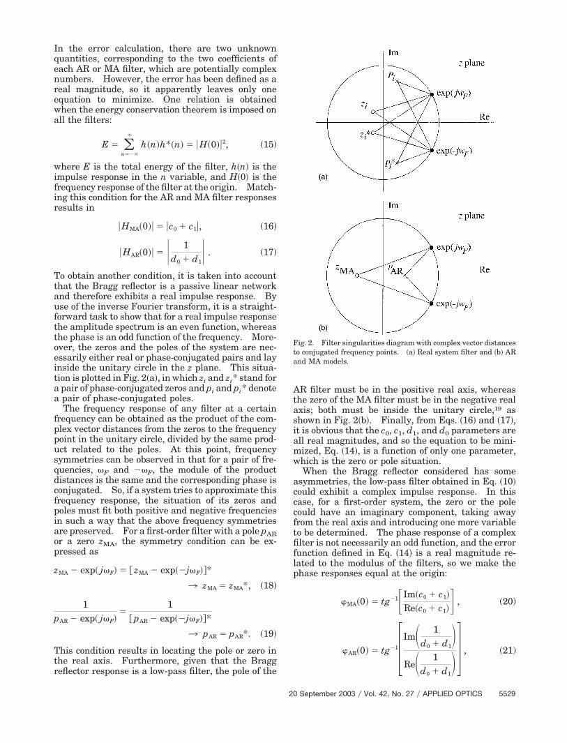
To obtain another condition, it is taken into accountthat the Bragg reflector is a passive linear networkand therefore exhibits a real impulse response. Byuse of the inverse Fourier transform, it is a straight-forward task to show that for a real impulse responsethe amplitude spectrum is an even function, whereasthe phase is an odd function of the frequency. More-over, the zeros and the poles of the system are nec-essarily either real or phase-conjugated pairs and layinside the unitary circle in the z plane. This situa-tion is plotted in Fig. 2�a�, in which zi and zi* stand fora pair of phase-conjugated zeros and pi and pi* denotea pair of phase-conjugated poles.

The frequency response of any filter at a certainfrequency can be obtained as the product of the com-plex vector distances from the zeros to the frequencypoint in the unitary circle, divided by the same prod-uct related to the poles. At this point, frequencysymmetries can be observed in that for a pair of fre-quencies, F and �F, the module of the productdistances is the same and the corresponding phase isconjugated. So, if a system tries to approximate thisfrequency response, the situation of its zeros andpoles must fit both positive and negative frequenciesin such a way that the above frequency symmetriesare preserved. For a first-order filter with a pole pARor a zero zMA, the symmetry condition can be ex-pressed as

zMA � exp� jF� � � zMA � exp��jF��*

3 zMA � zMA*, (18)

1pAR � exp� jF�

�1

� pAR � exp��jF��*

3 pAR � pAR*. (19)

This condition results in locating the pole or zero inthe real axis. Furthermore, given that the Braggreflector response is a low-pass filter, the pole of the

AR filter must be in the positive real axis, whereasthe zero of the MA filter must be in the negative realaxis; both must be inside the unitary circle,19 asshown in Fig. 2�b�. Finally, from Eqs. �16� and �17�,it is obvious that the c0, c1, d1, and d0 parameters areall real magnitudes, and so the equation to be mini-mized, Eq. �14�, is a function of only one parameter,which is the zero or pole situation.

When the Bragg reflector considered has someasymmetries, the low-pass filter obtained in Eq. �10�could exhibit a complex impulse response. In thiscase, for a first-order system, the zero or the polecould have an imaginary component, taking awayfrom the real axis and introducing one more variableto be determined. The phase response of a complexfilter is not necessarily an odd function, and the errorfunction defined in Eq. �14� is a real magnitude re-lated to the modulus of the filters, so we make thephase responses equal at the origin:

�MA�0� � tg�1�Im�c0 � c1�

Re�c0 � c1�� , (20)

�AR�0� � tg�1Im� 1d0 � d1

�Re� 1

d0 � d1� , (21)

Fig. 2. Filter singularities diagram with complex vector distancesto conjugated frequency points. �a� Real system filter and �b� ARand MA models.

20 September 2003 � Vol. 42, No. 27 � APPLIED OPTICS 5529

where Im and Re denote the imaginary and real partsof the complex numbers, respectively.

3. Numerical Results

For the purposes of showing the performance of theARMA modeling of Bragg reflectors, we take a typicalreflector as an example, which has 15 pairs of dielec-tric layers of alternated effective indices, 3.503 and2.95. The attenuation coefficient of the dielectriclayers, �s is equal to 10 cm�1, and the central wave-length of the electric field is placed in 1570 nm.These parameters are placed in Eq. �9� and solvediteratively through the 15 pairs of dielectric, result-ing in a digital filter of the form of Eq. �10�. Thefrequency band employed to obtain the coefficients ofthe AR and MA filters is limited to 12 THz, wideenough to contain any band used in WDM systems.The weighting function employed is uniform, with theaim of not prioritizing any frequency band. The co-efficients of the AR and MA filters, by use of Eq. �14�,are computed with fast Fourier transforms of 2048points, resulting in d0 � 1.663 and d1 � �0.653 forthe AR model and c0 � 0.502 and c1 � 0.487 for theMA model.

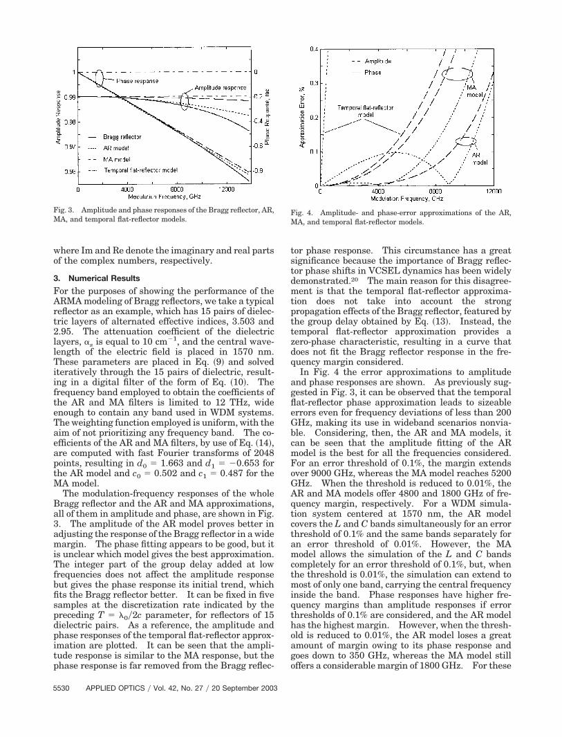
The modulation-frequency responses of the wholeBragg reflector and the AR and MA approximations,all of them in amplitude and phase, are shown in Fig.3. The amplitude of the AR model proves better inadjusting the response of the Bragg reflector in a widemargin. The phase fitting appears to be good, but itis unclear which model gives the best approximation.The integer part of the group delay added at lowfrequencies does not affect the amplitude responsebut gives the phase response its initial trend, whichfits the Bragg reflector better. It can be fixed in fivesamples at the discretization rate indicated by thepreceding T � �0�2c parameter, for reflectors of 15dielectric pairs. As a reference, the amplitude andphase responses of the temporal flat-reflector approx-imation are plotted. It can be seen that the ampli-tude response is similar to the MA response, but thephase response is far removed from the Bragg reflec-

tor phase response. This circumstance has a greatsignificance because the importance of Bragg reflec-tor phase shifts in VCSEL dynamics has been widelydemonstrated.20 The main reason for this disagree-ment is that the temporal flat-reflector approxima-tion does not take into account the strongpropagation effects of the Bragg reflector, featured bythe group delay obtained by Eq. �13�. Instead, thetemporal flat-reflector approximation provides azero-phase characteristic, resulting in a curve thatdoes not fit the Bragg reflector response in the fre-quency margin considered.

In Fig. 4 the error approximations to amplitudeand phase responses are shown. As previously sug-gested in Fig. 3, it can be observed that the temporalflat-reflector phase approximation leads to sizeableerrors even for frequency deviations of less than 200GHz, making its use in wideband scenarios nonvia-ble. Considering, then, the AR and MA models, itcan be seen that the amplitude fitting of the ARmodel is the best for all the frequencies considered.For an error threshold of 0.1%, the margin extendsover 9000 GHz, whereas the MA model reaches 5200GHz. When the threshold is reduced to 0.01%, theAR and MA models offer 4800 and 1800 GHz of fre-quency margin, respectively. For a WDM simula-tion system centered at 1570 nm, the AR modelcovers the L and C bands simultaneously for an errorthreshold of 0.1% and the same bands separately foran error threshold of 0.01%. However, the MAmodel allows the simulation of the L and C bandscompletely for an error threshold of 0.1%, but, whenthe threshold is 0.01%, the simulation can extend tomost of only one band, carrying the central frequencyinside the band. Phase responses have higher fre-quency margins than amplitude responses if errorthresholds of 0.1% are considered, and the AR modelhas the highest margin. However, when the thresh-old is reduced to 0.01%, the AR model loses a greatamount of margin owing to its phase response andgoes down to 350 GHz, whereas the MA model stilloffers a considerable margin of 1800 GHz. For these

Fig. 3. Amplitude and phase responses of the Bragg reflector, AR,MA, and temporal flat-reflector models.

Fig. 4. Amplitude- and phase-error approximations of the AR,MA, and temporal flat-reflector models.

5530 APPLIED OPTICS � Vol. 42, No. 27 � 20 September 2003

reasons, the AR model is appropriate for error thresh-olds of 0.1%, and the MA model gives a better approx-imation when the threshold is reduced to 0.01%.

This filter analysis could be extended to an ARMAfilter with both zeros and poles. For a first-ordersystem, however, the response is similar to that ob-tained with an AR model, given that the MA compo-nents always have lower entropy as compared withAR components.21 Moreover, the first-order ARMAfilter does not introduce error approximation advan-tages in the considered frequency bands. In addi-tion, one more coefficient must be determined, andthere is a loss of computing efficiency versus an ARmodel. From a physical point of view, the completeBragg reflector and the AR model are infinite-impulse-response filters, whereas the MA modeland the temporal flat-reflector approximation arefinite-impulse-response filters. The finite-impulse-response filters concentrate the energy of the pulsesin some finite samples along the temporal axis, wherethe temporal flat-reflector approximation is a limit tothis situation. In infinite-impulse-response filtersthe energy is dispersed along the temporal axis intoan infinite number of samples, tending to zero in theinfinite. To understand what is involved in this dif-ference, we should consider the laser operation re-gime. In a continuous-wave regime, both schemesare mathematically equivalent because the modula-tion around the central frequency is slow, whichmakes the discretization time of the digital filterssmall as compared with the modulated signals. Forself-pulsating lasers, however, the transient responseof the Bragg reflector has some importance,22 and thediscretization time of the digital filters is of the orderof the transient times of the pulses generated, spe-cially with ultrashort pulses. Usual parameterssuch as turn-on�off times cannot be modeled accu-rately with low-order MA filters because the energy isconcentrated in some finite samples; thus they do notplay a physical role in the Bragg reflector, making itnecessary to consider AR components in the Braggreflector approximations. In such a case, ARMA fil-ters of orders from above are interesting but requirespecific methods for the minimization of the approx-imation errors, owing to the greater number of coef-ficients to be determined.

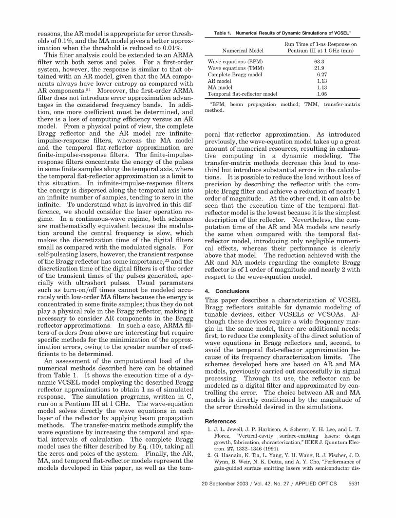
An assessment of the computational load of thenumerical methods described here can be obtainedfrom Table 1. It shows the execution time of a dy-namic VCSEL model employing the described Braggreflector approximations to obtain 1 ns of simulatedresponse. The simulation programs, written in C,run on a Pentium III at 1 GHz. The wave-equationmodel solves directly the wave equations in eachlayer of the reflector by applying beam propagationmethods. The transfer-matrix methods simplify thewave equations by increasing the temporal and spa-tial intervals of calculation. The complete Braggmodel uses the filter described by Eq. �10�, taking allthe zeros and poles of the system. Finally, the AR,MA, and temporal flat-reflector models represent themodels developed in this paper, as well as the tem-

poral flat-reflector approximation. As introducedpreviously, the wave-equation model takes up a greatamount of numerical resources, resulting in exhaus-tive computing in a dynamic modeling. Thetransfer-matrix methods decrease this load to one-third but introduce substantial errors in the calcula-tions. It is possible to reduce the load without loss ofprecision by describing the reflector with the com-plete Bragg filter and achieve a reduction of nearly 1order of magnitude. At the other end, it can also beseen that the execution time of the temporal flat-reflector model is the lowest because it is the simplestdescription of the reflector. Nevertheless, the com-putation time of the AR and MA models are nearlythe same when compared with the temporal flat-reflector model, introducing only negligible numeri-cal effects, whereas their performance is clearlyabove that model. The reduction achieved with theAR and MA models regarding the complete Braggreflector is of 1 order of magnitude and nearly 2 withrespect to the wave-equation model.

4. Conclusions

This paper describes a characterization of VCSELBragg reflectors suitable for dynamic modeling oftunable devices, either VCSELs or VCSOAs. Al-though these devices require a wide frequency mar-gin in the same model, there are additional needs:first, to reduce the complexity of the direct solution ofwave equations in Bragg reflectors and, second, toavoid the temporal flat-reflector approximation be-cause of its frequency characterization limits. Theschemes developed here are based on AR and MAmodels, previously carried out successfully in signalprocessing. Through its use, the reflector can bemodeled as a digital filter and approximated by con-trolling the error. The choice between AR and MAmodels is directly conditioned by the magnitude ofthe error threshold desired in the simulations.

References1. J. L. Jewell, J. P. Harbison, A. Scherer, Y. H. Lee, and L. T.

Florez, “Vertical-cavity surface-emitting lasers: designgrowth, fabrication, characterization,” IEEE J. Quantum Elec-tron. 27, 1332–1346 �1991�.

2. G. Hasnain, K. Tia, L. Yang, Y. H. Wang, R. J. Fischer, J. D.Wynn, B. Weir, N. K. Dutta, and A. Y. Cho, “Performance ofgain-guided surface emitting lasers with semiconductor dis-

Table 1. Numerical Results of Dynamic Simulations of VCSELa

Numerical ModelRun Time of 1-ns Response on

Pentium III at 1 GHz �min�

Wave equations �BPM� 63.3Wave equations �TMM� 21.9Complete Bragg model 6.27AR model 1.13MA model 1.13Temporal flat-reflector model 1.05

aBPM, beam propagation method; TMM, transfer-matrixmethod.

20 September 2003 � Vol. 42, No. 27 � APPLIED OPTICS 5531

tributed Bragg reflector,” IEEE J. Quantum Electron. 27,1377–1385 �1991�.

3. R. Lewen, K. Streubel, A. Karlsson, and S. Rapp, “Experimen-tal demonstration of a multifunctional long-wavelengthvertical-cavity laser amplifier-detector,” IEEE Photon. Tech-nol. Lett. 10, 1067–1069 �1998�.

4. D. Wiedenmann, B. Moeller, R. Michalzik, and K. J. Ebeling,“Performance characteristics of vertical-cavity semiconductorlaser amplifiers,” IEE Electron. Lett. 32, 342–343 �1996�.

5. J. Piprek, S. Bjorlin, and J. E. Bowers, “Design and analysis ofvertical-cavity semiconductor optical amplifiers,” IEEE J.Quantum Electron. 37, 127–134 �2001�.

6. K. A. Black, E. S. Bjorlin, J. Piprek, E. L. Hu, and J. E. Bowers,“Small-signal frequency response of long-wavelength vertical-cavity lasers,” IEEE Photon. Technol. Lett. 13, 1049–1051�2001�.

7. C. J. Chang-Hasnain, “Tunable VCSEL,” IEEE J. Sel. Top.Quantum Electron. 6, 978–987 �2000�.

8. M. S. Wu, E. C. Vail, G. S. Li, W. Yuen, and C. J. Chang-Hasnain, “Tunable micromachined vertical cavity surfaceemitting laser,” IEE Electron. Lett. 31, 1671–1672 �1995�.

9. D. I. Babic, Y. Chung, N. Dagli, and J. E. Bowers, “Modalreflection of quarter-wave mirrors in vertical-cavity lasers,”IEEE J. Quantum Electron. 29, 1950–1962 �1993�.

10. S. F. Yu, “Dynamic behavior of vertical-cavity surface-emittinglasers,” IEEE J. Quantum Electron. 32, 1168–1179 �1996�.

11. D. I. Babic and S. W. Corzine, “Analytic expressions for thereflection delay, penetration depth, and absorptance ofquarter-wave dielectric mirrors,” IEEE J. Quantum Electron.28, 514–524 �1992�.

12. S. F. Yu, “An improved time-domain traveling-wave model forvertical-cavity surface-emitting lasers,” IEEE J. QuantumElectron. 34, 1938–1948 �1998�.

13. J. F. P. Seurin and S. L. Chuang, “Discrete Bessel transformand beam propagation method for modeling of vertical-cavitysurface-emitting lasers,” J. Appl. Phys. 82, 2007–2016 �1997�.

14. S. F. Yu, “Nonlinear dynamics of vertical-cavity surface-emitting lasers,” IEEE J. Quantum Electron. 35, 332–341�1999�.

15. L. R. Rabiner and R. W. Schafer, Digital Processing of SpeechSignals �Prentice-Hall, New York, 1979�.

16. S. F. Yu and C. W. Lo, “Influence of transverse modes on thedynamic response of vertical cavity surface emitting lasers,”IEE Proc. Optoelectron. 143, 189–194 �1996�.

17. A. Mossakowska, P. Witonski, and P. Szczepanski, “Relaxationoscillations in a laser with a Gaussian mirror,” Appl. Opt. 41,1668–1676 �2002�.

18. S. Ramo, J. R. Whinnery, and T. Van Duzer, Fields and Wavesin Communications Electronics �Wiley, New York, 1994�.

19. J. G. Proakis and D. G. Manolakis, Introduction to DigitalSignal Processing �MacMillan, New York, 1988�.

20. J. P. Ziang and K. Petermann, “Beam propagation for vertical-cavity surface-emitting lasers: threshold properties,” IEEEJ. Quantum Electron. 30, 1529–1536 �1994�.

21. W. H. Press, S. A. Teukolsky, W. T. Vetterling, and B. P.Flannery, Numerical Recipes in C: the Art of Scientific Com-puting �Cambridge U. Press, Cambridge, UK, 1993�.

22. C. G. Lim, S. Iekeziel, and C. M. Snowden, “Nonlinear dynam-ics of optically injected self-pulsating laser diodes,” IEEE J.Quantum Electron. 37, 699–706 �2001�.

5532 APPLIED OPTICS � Vol. 42, No. 27 � 20 September 2003