HAL Id: insu-01467174https://hal-insu.archives-ouvertes.fr/insu-01467174

Submitted on 14 Feb 2017

HAL is a multi-disciplinary open accessarchive for the deposit and dissemination of sci-entific research documents, whether they are pub-lished or not. The documents may come fromteaching and research institutions in France orabroad, or from public or private research centers.

L’archive ouverte pluridisciplinaire HAL, estdestinée au dépôt et à la diffusion de documentsscientifiques de niveau recherche, publiés ou non,émanant des établissements d’enseignement et derecherche français ou étrangers, des laboratoirespublics ou privés.

Wide-band, low-frequency pulse profiles of 100 radiopulsars with LOFAR

M. Pilia, J.W.T. Hessels, B.W Stappers, V.I. Kondratiev, M Kramer, J vanLeeuwen, P Weltevrede, A Lyne, K Zagkouris, T.E. Hassall, et al.

To cite this version:M. Pilia, J.W.T. Hessels, B.W Stappers, V.I. Kondratiev, M Kramer, et al.. Wide-band, low-frequencypulse profiles of 100 radio pulsars with LOFAR. Astronomy and Astrophysics - A&A, EDP Sciences,2016, 586 (A92), 34 p. �10.1051/0004-6361/201425196�. �insu-01467174�

A&A 586, A92 (2016)DOI: 10.1051/0004-6361/201425196c© ESO 2016

Astronomy&

Astrophysics

Wide-band, low-frequency pulse profiles of 100 radio pulsarswith LOFAR�

M. Pilia1,2, J. W. T. Hessels1,3, B. W. Stappers4, V. I. Kondratiev1,5, M. Kramer6,4, J. van Leeuwen1,3, P. Weltevrede4,A. G. Lyne4, K. Zagkouris7, T. E. Hassall8, A. V. Bilous9, R. P. Breton8, H. Falcke9,1, J.-M. Grießmeier10,11,

E. Keane12,13, A. Karastergiou7, M. Kuniyoshi14, A. Noutsos6, S. Osłowski15,6, M. Serylak16, C. Sobey1, S. ter Veen9,A. Alexov17, J. Anderson18, A. Asgekar1,19, I. M. Avruch20,21, M. E. Bell22, M. J. Bentum1,23, G. Bernardi24,

L. Bîrzan25, A. Bonafede26, F. Breitling27, J. W. Broderick7,8, M. Brüggen26, B. Ciardi28, S. Corbel29,11, E. de Geus1,30,A. de Jong1, A. Deller1, S. Duscha1, J. Eislöffel31, R. A. Fallows1, R. Fender7, C. Ferrari32, W. Frieswijk1,

M. A. Garrett1,25, A. W. Gunst1, J. P. Hamaker1, G. Heald1, A. Horneffer6, P. Jonker20, E. Juette33, G. Kuper1, P. Maat1,G. Mann27, S. Markoff3, R. McFadden1, D. McKay-Bukowski34,35, J. C. A. Miller-Jones36, A. Nelles9, H. Paas37,

M. Pandey-Pommier38, M. Pietka7, R. Pizzo1, A. G. Polatidis1, W. Reich6, H. Röttgering25, A. Rowlinson22,D. Schwarz15, O. Smirnov39,40, M. Steinmetz27, A. Stewart7, J. D. Swinbank41, M. Tagger10, Y. Tang1, C. Tasse42,

S. Thoudam9, M. C. Toribio1, A. J. van der Horst3, R. Vermeulen1, C. Vocks27, R. J. van Weeren24, R. A. M. J. Wijers3,R. Wijnands3, S. J. Wijnholds1, O. Wucknitz6, and P. Zarka42

(Affiliations can be found after the references)

Received 20 October 2014 / Accepted 18 September 2015

ABSTRACT

Context. LOFAR offers the unique capability of observing pulsars across the 10−240 MHz frequency range with a fractional bandwidth of roughly50%. This spectral range is well suited for studying the frequency evolution of pulse profile morphology caused by both intrinsic and extrinsiceffects such as changing emission altitude in the pulsar magnetosphere or scatter broadening by the interstellar medium, respectively.Aims. The magnitude of most of these effects increases rapidly towards low frequencies. LOFAR can thus address a number of open questionsabout the nature of radio pulsar emission and its propagation through the interstellar medium.Methods. We present the average pulse profiles of 100 pulsars observed in the two LOFAR frequency bands: high band (120–167 MHz, 100 pro-files) and low band (15–62 MHz, 26 profiles). We compare them with Westerbork Synthesis Radio Telescope (WSRT) and Lovell Telescopeobservations at higher frequencies (350 and 1400 MHz) to study the profile evolution. The profiles were aligned in absolute phase by folding witha new set of timing solutions from the Lovell Telescope, which we present along with precise dispersion measures obtained with LOFAR.Results. We find that the profile evolution with decreasing radio frequency does not follow a specific trend; depending on the geometry of thepulsar, new components can enter into or be hidden from view. Nonetheless, in general our observations confirm the widening of pulsar profiles atlow frequencies, as expected from radius-to-frequency mapping or birefringence theories.

Key words. stars: neutron – pulsars: general

1. Introduction

The cumulative (i.e. average) pulse profiles of radio pulsars arethe sum of hundreds to thousands of individual pulses, and are,loosely speaking, a unique signature of each pulsar (Lorimer2008). They are normally stable in their morphology and arereproducible, although several types of variation have been ob-served both for non-recycled pulsars (see Helfand et al. 1975;Weisberg et al. 1989; Rathnasree & Rankin 1995 and Lyne et al.2010) and for millisecond pulsars (Liu et al. 2012). For mostpulsars, this cumulative pulse profile morphology often varies(sometimes drastically, sometimes subtly) as a function of ob-serving frequency because of a number of intrinsic effects (e.g.emission location in the pulsar magnetosphere) and extrinsic

� We offer this catalogue of low-frequency pulsar profiles in a userfriendly way via the EPN Database of Pulsar Profiles, http://www.epta.eu.org/epndb/

effects (i.e. due to propagation in the interstellar medium; ISM),see for instance Cordes (1978). As Fig. 1 shows, pulse profileevolution can become increasingly evident at the lowest observ-ing frequencies (<200 MHz).

Mapping profile evolution over a wide range of frequenciescan aid in modelling the pulsar radio emission mechanism itself(see e.g. Rankin 1993 and related papers of the series) and con-straining properties of the ISM (e.g. Hassall et al. 2012). Sincemany of the processes that affect the pulse shape strongly dependon the observing frequency, observations at low frequencies pro-vide valuable insights on them. The LOw-Frequency ARray(LOFAR) is the first telescope capable of observing nearly theentire radio spectrum in the 10−240 MHz frequency range, thelowest 4.5 octaves of the “radio window” (van Haarlem et al.2013) and (Stappers et al. 2011).

Low-frequency pulsar observations have previously beenconducted by a number of telescopes, (e.g. Gauribidanur Radio

Article published by EDP Sciences A92, page 1 of 34

A&A 586, A92 (2016)

Fig. 1. Example of pulsar profile evolution for PSR B0950+08,from 1400 MHz down to 30 MHz. It becomes more rapid at low fre-quencies. The bars on the left represent the intra-channel smearing dueto uncorrected DM delay within a channel at each frequency. The pro-files were aligned using a timing ephemeris (see text for details).

Telescope (GEETEE): Asgekar & Deshpande 1999; LargePhased Array Radio Telescope, Puschino: Kuzmin et al.(1998), Malov & Malofeev 2010; Arecibo: Hankins & Rankin2010; Ukrainian T-shaped Radio telescope, second modifica-tion (UTR-2): Zakharenko et al. 2013), and simultaneous ef-forts are being undertaken by other groups in parallel (e.g.Long Wavelength Array (LWA): Stovall et al. 2015, MurchisonWidefield Array (MWA): Tremblay et al. 2015). Nevertheless,LOFAR offers several advantages over the previous studies.Firstly, the large bandwidth that can be recorded at any giventime (48 MHz in 16-bit mode and 96 MHz in 8-bit mode) allowsfor continuous wide-band studies of the pulse profile evolution,compared to studies using a number of widely separated, narrowbands (e.g. the 5×32 and 20×32 kHz bands used at 102 MHz in

Kuzmin et al. 1998). Secondly, LOFAR’s ability to track sourcesis also an advantage, as many pulses can be collected in a singleobserving session instead of having to combine several short ob-servations in the case of transit instruments (e.g. Izvekova et al.1989). This eliminates systematic errors in the profile that aredue to imprecise alignment of the data from several observingsessions. Thirdly, LOFAR can achieve greater sensitivity by co-herently adding the signals received by individual stations, giv-ing a collecting area equivalent to the sum of the collecting areaof all stations (up to 57 000 m2 at HBAs and 75 200 m2 at LBAs,see Stappers et al. 2011). Finally, LOFAR offers excellent fre-quency and time resolution. This is necessary for dedispersingthe data to resolve narrow features in the profile. LOFAR is alsocapable of coherently dedispersing the data, although that modewas not employed here.

As mentioned above, there are two types of effects thatLOFAR will allow us to study with great precision. One of theseare extrinsic effects related to the ISM. Specifically, the ISMcauses scattering and dispersion. Mean scatter-broadening (as-suming a Kolmogorov distribution of the turbulence in the ISM)scales with observing frequency as ν−4.4. The scattering causesdelays in the arrival time of the emission at Earth, which can bemodelled as having an exponentially decreasing probability ofbeing scattered back into our line-of-sight: this means that theintensity of the pulse is spread in an exponentially decreasingtail. Dispersion scales as ν−2 and is mostly corrected for by chan-nelising and dedispersing the data (see e.g. Lorimer & Kramer2004). Nonetheless, for filterbank (channelised) data some resid-ual dispersive smearing persists within each channel:

tDM = 8.3 · DMΔν

ν3μs, (1)

where DM is the dispersion measure in cm−3 pc, Δν is the chan-nel width in MHz, and ν the central observing frequency in GHz.This does not significantly affect the profiles that we present here(at least not at frequencies above ∼50 MHz) because the pulsarsstudied have low DMs and the data are chanellised in narrow fre-quency channels (see Sect. 2). Second-order effects in the ISMmay also be present, but have yet to be confirmed. For instance,previous claims of “super-dispersion”, meaning a deviation fromthe ν−2 scaling law (see e.g. Kuz’min et al. 2008 and referencestherein), were not observed by Hassall et al. (2012), with an up-per limit of <∼50 ns at a reference frequency of 1400 MHz.

The second type of effects under investigation are those in-trinsic to the pulsar. One of the most well-known intrinsic ef-fects are pulse broadening at low frequencies, which has beenobserved in many pulsars (e.g. Hankins & Rickett 1986 andMitra & Rankin 2002), while others show no evidence of this(e.g. Hassall et al. 2012). One of the theories explaining thiseffect is radius-to-frequency mapping (RFM, Cordes 1978): itpostulates that the origin of the radio emission in the pulsar’smagnetosphere increases in altitude above the magnetic polestowards lower frequencies. RFM predicts that the pulse profilewill increase in width towards lower observing frequency, sinceemission will be directed tangentially to the diverging magneticfield lines of the magnetosphere that corotates with the pulsar.An alternative interpretation (McKinnon 1997) proposes bire-fringence of the plasma above the polar caps as the cause forbroadening: the two propagation modes split at low frequencies,causing the broadening, while they stay closer together at highfrequencies, causing depolarisation (this is investigated in theLOFAR work on pulsar polarisation, see Noutsos et al. 2015).

In this paper, we present the average pulse profilesof 100 pulsars observed in two LOFAR frequency ranges: high

A92, page 2 of 34

M. Pilia et al.: LOFAR 100 pulsar profiles

band (119–167 MHz, 100 profiles) and low band (15–62 MHz,26 out of the 100 profiles). We compare the pulse profile mor-phologies with those obtained around 350 and 1400 MHz withthe WSRT and Lovell telescopes, respectively, to study their evo-lution with respect to a magnetospheric origin and DM-inducedvariations. We do not discuss here profile evolution due to theeffects of scattering in the ISM, which will be the target of afuture work (Zagkouris et al., in prep.). In Sect. 2 we describethe LOFAR observational setup and parameters. In Sect. 3 wedescribe the analysis. In Sect. 4 we discuss the results, and inSect. 5 we conclude with some discussion on future extensionsof this work.

2. Observations

The observed sample of pulsars was loosely based on a selec-tion of the brightest objects in the LOFAR-visible sky (decli-nation >−30◦), using the ATNF Pulsar Catalog1 (Manchesteret al. 2005) for guidance. Because pulsar flux and spectral in-dices are typically measured at higher frequencies, we also basedour selection on the previously published data at low frequen-cies (Malov & Malofeev 2010). Since the LOFAR dipoles havea sensitivity that decreases as a function of the zenith angle, allsources were observed as close to transit as possible, and onlythe very brightest sources south of the celestial equator wereobserved.

We observed 100 pulsars using the high-band antennas(HBAs) in the six central “Superterp” stations (CS002−CS007)of the LOFAR core2. The observations were performed in tied-array mode, that is, a coherent sum of the station signals us-ing appropriate geometrical and instrumental phase and timedelays (see Stappers et al. 2011 for a detailed description ofLOFAR’s pulsar observing modes and van Haarlem et al. 2013for a general description of LOFAR). The 119−167-MHz fre-quency range was observed using 240 subbands of 195 kHzeach, synthesised at the station level, where the individual HBAtiles were combined to form station beams. Using the LOFARBlue Gene/P correlator, each subband was further channelisedinto 16 channels, formed into a tied-array beam. The linear po-larisations were summed in quadrature (pseudo-Stokes I), andthe signal intensity was written out as 245.76μs samples. Theintegration time of each observation was at least 1020 s. Thiswas chosen to provide an adequate number of individual pulses,so as to average out the absolute scale of the variance associ-ated with pulse-phase “jitter” to the cumulative profile. The jitter,also termed stochastic wide-band impulse modulated self-noise(SWIMS, as in Osłowski et al. 2011), is the variation in indi-vidual pulse intensity and position with respect to the averagepulse profile (see also Cordes 1993 and Liu et al. 2012 and ref-erences therein). This variation does not significantly affect themeasurements that have been carried out for the scope of thispaper (i.e. pulse widths, peak heights), but we have checked thatthe resulting profile was stable on the considered time scales bydividing each observation into shorter sections and comparingthe shapes of the resulting profiles with the overall profile. In thecases where stability was not achieved, we used longer integra-tion times. Regardless, in almost all cases the profile evolutionwith observing frequency is a significantly stronger effect at lowfrequencies.

1 http://www.atnf.csiro.au/people/pulsar/psrcat/2 The full LOFAR Core can now be used for observations and pro-vides four times the number of stations available on the Superterp (anda proportional increase in sensitivity).

Twenty-six of the brightest pulsars were also observed us-ing the Superterp low-band antennas (LBAs) in the frequencyrange 15−62 MHz. To mitigate the larger dispersive smearingof the profile in this band, 32 channels were synthesised foreach of the 240 subbands. The sampling time was 491.52μs.The integration time of these observations was increased to atleast 2220 s to somewhat compensate for the lower sensitivity atthis frequency band (e.g. because of the higher sky temperature).

For some sources, 17-minute HBA observations with theSuperterp were insufficient to achieve acceptable signal-to-noise(S/N) profiles. For these, longer integration times (or morestations) were needed. Hence, some of the pulsars presentedhere were later observed with 1 hr pointings as part of theLOFAR Tied-Array All-Sky Survey for pulsars and fast tran-sients (LOTAAS3: see also Coenen et al. 2014), which com-menced after the official commissioning period, during Cycle 0of LOFAR scientific operations, and is currently ongoing.LOTAAS combines multiple tied-array beams (219 total) perpointing to observe both a survey grid as well as known pulsarswithin the primary field-of-view.

3. Analysis

The LOFAR HDF54 (Hierarchical Data Format5, see e.g., Alexovet al. 2010) data were converted to PSRFITS format (Hotan et al.2004) for further processing. Radio frequency interference (RFI)was excised by removing affected time intervals and frequencychannels, using the tool rfifind from the PRESTO5 softwaresuite (Ransom 2001). The data were dedispersed and folded us-ing PRESTO and, in a first iteration, a rotational ephemeris fromthe ATNF pulsar catalogue, using the automatic LOFAR pul-sar pipeline “PulP”. The number of bins across each profile waschosen so that each bin corresponds to approximately 1.5 ms.

The profiles obtained with the HBA and, where available,LBA bands were compared with the profiles obtained withthe WSRT at ∼350 MHz (from here onwards “P-band”) andat ∼1400 MHz, or with the Lovell Telescope at the Jodrell BankObservatory at ∼1500 MHz (from here onwards “L-band”). TheWSRT observations that we used were performed mostly be-tween 2003 and 2004 (see Weltevrede et al. 2006, “WES” fromhere onwards, and Weltevrede et al. 2007 for details). The Lovellobservations were all contemporary to LOFAR observations,therefore in the cases where both sets of observations were avail-able, we chose the Lovell ones because they are closer to oroverlap the epoch of the LOFAR observations. At L-band weused Lovell observations for all but three pulsars: B0136+57,B0450−18, and B0525+21. In a handful of cases, where no pro-file at P-band was available from WES, we used the data fromthe European Pulsar Network (EPN) database6.

To attempt to align the data absolutely, we generatedephemerides that spanned the epochs of the observations thatwere used. This did not include those from the EPN database,however. Ephemerides were generated from the regular moni-toring observations made with the Lovell Telescope. The timesof arrival were generated using data from an analogue filterbank(AFB) up until January 2009 and a digital filterbank (DFB) sincethen, with a typical observing cadence between 10 and 21 days.The observing bandwidth was 64 MHz at a central frequency

3 http://www.astron.nl/lotaas/4 http://www.hdfgroup.org/HDF5/5 https://github.com/scottransom/presto6 http://www.epta.eu.org/epndb/

A92, page 3 of 34

A&A 586, A92 (2016)

of 1402 MHz and approximately 380 MHz at a central fre-quency of 1520 MHz for the AFB and DFB, respectively. Theephemerides were generated using a combination of PSRTIME7

and TEMPO, and in the case of those pulsars demonstrating ahigh degree of timing noise, up to five spin-frequency deriva-tives were fit to ensure white residuals and thus good phasealignment.

The L-band profiles were generated from DFB observationsby forming the sum of up to a dozen observations, aligned usingthe same ephemerides used to align the multi-frequency data. Were-folded both the LOFAR and the high frequency data sets us-ing this ephemeris. In general, where Lovell data were available,the ephemeris was created using about 100 days’ worth of data.For the WSRT observations, an ephemeris was created spanning,in some cases, ten years of data and ending at the time of theLOFAR observations. The timing procedure was the same as forthe shorter data spans, except that astrometric parameters werefit and typically more spin-frequency derivatives were required.The epoch of the WSRT observations is specified in Table B.1in the Notes column. Given the method we used to align the pro-files, the timing solution is less accurate over these longer timespans than those constructed to align the Lovell data, but thistoo represents a good model, with a standard deviation (rms) ofthe timing residuals <∼1 ms. We aligned the profiles in absolutephase by calculating the phase shift between the reference epochof the observations and the reference epoch of the ephemeris andapplying this phase shift to each data set.

Some of the pulsar parameters derived from theseephemerides are presented in Table B.1. The first column liststhe observed pulsars, the second and third columns list the spinperiod and period derivative of each pulsar, the fourth column isthe reference epoch of the rotational ephemeris that was used tofold the data, and Cols. 5 and 6 list the epochs of the LOFARHBA and LBA observations. In Cols. 7 and 8 two measurementsfor the DM are given: the first as originally used to dedispersethe observations at higher frequencies, and the second as the bestDM obtained from the fit of the HBA LOFAR observations usingPRESTO’s prepfold (Ransom 2001). The next three columnsprovide the pulsar’s spin-down age, magnetic field strength, andspin-down luminosity as derived from the rotational parame-ters according to standard approximations (see e.g. Lorimer &Kramer 2004):

τ[s] = 0.5P/P, (2)

B[G] = 3.219 × 1019√

PP, (3)

E[erg/s] = 4π2 × 1045P/P3, (4)

where P is measured in s and P in s s−1. The resulting alignedprofiles for the 100 pulsars are shown in Fig. B.1 in Appendix B.The star next to the name of the band (P-band in most cases,with the exception of B0136+57, where we used the P-bandfor absolute alignment) indicates that the corresponding bandwas aligned by eye based on the absolute alignment betweenthe LOFAR data and the other high-frequency band. The align-ment was made based only on the choice of a specific pointalong the rotational phase of the pulsar, at the reference epochof the ephemeris, but unmodelled DM variations can be respon-sible for extra, albeit small, phase shifts (up to a few percent, seeTable 1). Indeed, observations performed at different times, quitefar apart, and at different frequencies, can possess quite differ-ent apparent DMs (up to some tenth of a percent, see Table 1).

7 http://www.jb.man.ac.uk/~pulsar/observing/progs/psrtime.html

Table 1. Pulsars for which the absolute alignment was not achieved withthe refolding using the same ephemeris (see text for details).

PSR Name Extra DM shift/causes for misalignmentB0114+58 SB0525+21 F4, S, gB1633+24 F4, rms = 1.3, DM = −0.11, Δφ = 0.043B1818−04 SB1839+09 rms = 1.4, DM = −0.13, Δφ = 0.051B1848+13 DM = −0.04, Δφ = 0.017B1907+10 F3, SB1915+13 SB2148+63 S

Notes. The extra DM shift (in cm−3 pc) and corresponding phaseshift (Δφ) needed to align the profiles are indicated, or possibly otherreasons for the observed shift, e.g., S for scattering, which notably al-ters the shape of the profile, g in case a glitch occurred during the rangeof the ephemeris, number of spin-frequency derivatives fitted to obtain agood ephemeris (i.e. F#), or final rms (in ms) of the best timing solution.

DMs that are due to the ISM have, as expected, a time depen-dence (see You et al. 2007; Keith et al. 2013), and these differ-ences can become quite relevant especially at the lowest LOFARfrequencies. We chose to re-dedisperse all the profiles, LOFARand high-frequency ones, using the DM obtained as the best DMwith prepfold for the HBA LOFAR observations. prepfolddetermines an optimum DM by sliding frequency subbands withrespect to each other to maximise the S/N of the cumulative pro-file. The intra-channel smearing caused by DM over the band-width at the centre frequency is indicated by the filled rectanglenext to each profile in Fig. B.1.

Only in a few cases, documented in Table 1, was the DM ob-tained from the LOFAR observations not used for the alignment.Those are the cases for which, also evident from Fig. B.1, theintra-channel smearing caused by DM is a substantial fractionof the profile width (similar to or higher than the on-pulse re-gion), and therefore the quality of the measurement is lowerthan that obtained at a higher observing frequency. On the otherhand, in some other cases (although rare, see Table B.1), eventhe LBA measurement was good enough to provide a DM mea-surement, and in these cases we were able to use that for thealignment. In this way we obtain the best alignments, in general,even though some residual offsets could still be observed in ahandful of cases.

For those cases (listed in Table 1) where the remaining off-set was noticeable by eye, we investigated the possible causesafter refolding and applying the new DM. We checked whetherthe pulsars in our sample had undergone any glitch activity dur-ing the time spanned by our ephemerides. Sixteen out of our100 pulsars have shown glitch activity at some time. Seven ofthem have experienced glitches relatively close to the epoch ofour observations, but only two of them during the time spannedby our ephemerides. The relevant glitch epochs of these pulsarsare presented in Table 2 and were taken from the Jodrell Bankglitch archive8 (Espinoza et al. 2011, 2012), integrated with theATNF pulsar archive9. We note that while the glitch activitycould have had an influence on the shift of PSR B0525+21, therecurrent activity of PSR B0355+54 did not cause as notable an

8 http://www.jb.man.ac.uk/pulsar/glitches/gTable.html9 http://www.atnf.csiro.au/people/pulsar/psrcat/glitchTbl.html

A92, page 4 of 34

M. Pilia et al.: LOFAR 100 pulsar profiles

Table 2. Pulsars for which one or more glitches occurred during therange of the ephemerides used in this paper (above the horizontal line)or near the range of validity of our ephemerides (below the horizontalline).

PSR Name Start End Glitch epoch

[MJD] [MJD] [MJD]

B0355+54 51 364.6 56 262.2 51 679(15)[1]

51 969(1)[1]

52 943(3)[1]

53 209(2)[1]

B0525+21 52 274.9 56 641.1 52 296(1)[2,3]

53 379[2]

53 980(12)[3]

B0919+06 55 555.2 56 557.5 55 152(6)[1]

B1530+27 51 607.0 56 535.6 49 732(3)[1]

B1822−09 54 876.5 56 571.8 54 114.96(3)[1]

B1907+00 54 984.1 56 556.9 53 546(2)[1]

B1907+10 54 924.5 56 535.1 54 050(350 [s])[3]

B2224+65 55 359.7 56 570.1 54 266(14)[2,3]

B2334+61 54 635.4 56 507.3 53 642(13)[1,3]

Notes. The uncertainty of the glitch epoch is quoted in parentheses andit is expressed in days, except for the case of PSR B1907+10, where itis quoted in seconds. Sources: Jodrell Bank and ATNF glitch archives.

References. [1] Espinoza et al. (2011); [2] Janssen & Stappers (2006);[3] Yuan et al. (2010).

impact on the alignment. In some cases the profile is scatteredin the LOFAR HBA band and rapidly becomes more scatteredtowards lower frequencies. This will affect the accuracy of theDM measurement, potentially causing an extra profile shift be-tween bands. In some cases the ephemeris had a large rms timingresidual, or it included higher order spin-frequency derivativesbeyond the second, which is typical of unstable, “noisy” pulsars.All these cases are indicated in Table 1. In the other cases, wecalculated that a DM difference <∼0.05 cm−3 pc, compatible withthe measurement uncertainties, would compensate for that shift.For this reason, we applied an extra shift to align these pulsars’profiles by eye in Fig. B.1 and referenced this shift in Table 1.

Only a small number of pulsars in our sample show in-terpulses: B0823+26, B0950+08, B1822–09, B1929+10, andB2022+50. For these pulsars the profile longitude is shown inits entire phase range instead of in the phase interval 0.25−0.75,as was chosen for the other profiles. The phase-aligned pro-files, which normally have their reference point at 0.5, have beenshifted by+0.25 in these cases, to help the visualisation of the in-terpulse. A zoom-in of the interpulse region is shown in Fig. B.2(LBA data were excluded because none of the interpulses weredetected in that band). Our sample also contains a few modingpulsars (notably B0823+26 and B0943+10). For these pulsarswe caution that the profile reflects only the mode observed inthe particular observations presented here. A more detailed treat-ment of the low-frequency profiles of B0823+26 and B0943+10can be found in Sobey et al. (2015) and Bilous et al. (2014), re-spectively. In yet other cases, for instance B1857–26, no modingbehaviour has previously been documented, but notable changesin the profile are seen from high to low frequencies. Thesemight reflect different modes of emission when the various

observations were taken. A more detailed discussion of somecases of peculiar profile evolution can be found in Sect. 5.3.

We fit the multi-band profiles of each pulsar using Gaussiancomponents (see an example in Fig. 2), which are a good repre-sentation for the profiles of slow pulsars (see Kramer et al. 1994and references therein). We used the program pygaussfit.py,of the PRESTO suite, which has the advantage of providing an in-teractive basis for the input parameters to the Gaussian fits. Thisprogram can be used to apply the same method as in Krameret al. (1994; see e.g. Fig. 3 of their paper), as it provides post-fitresiduals (for the discrepancy between the model and the data,see bottom half-plots of Fig. 2) that we required to have approx-imately the same distribution in the on-pulse as in the off-pulseregion. The full rotational period, and not only the on-pulse re-gion, was taken into account by the fit, also allowing for distin-guishing interpulses or small peaks at different phases from thenoise. The Gaussian components derived using this method werechosen to satisfy the condition of best fit with minimal redun-dancy, and no physical significance should be attributed to them.Hassall et al. (2012) have shown that it is possible to accuratelymodel the evolution of the profile with frequency using Gaussiancomponents, but a specific model has to be applied individuallyto each pulsar, requiring much careful consideration. Such ananalysis is beyond the scope of this paper. In the absence of amore comprehensive treatment of scattering for LOFAR profiles,which is envisaged for subsequent papers, the most evident scat-tering tails of the low-frequency profiles have not been modelledand the corresponding profiles components were not included inthe table and are not used in any further analysis.

We used the mathematical description of the profiles in termsof the Gaussian components to calculate the widths and ampli-tudes of the observed peaks. For each profile we obtained thefull width at half maximum (w50) and the full width at 10% ofthe maximum, w10. To calculate the errors on the widths, wesimulated 1000 realisations of each profile, using the noiselessGaussian-based template and adding noise with a standard devi-ation equal to that measured in the off-pulse region of the ob-served profile. By measuring the widths in these realisations,we obtained a distribution of allowed widths from which wedetermined their standard deviation. We note that these errorsare statistical only and do not take into account the validity ofour assumptions, that is, the reliability of the template used.To cross-check the width of the full profile, we tried differentmethods. An example of how these widths were calculated isdescribed in Appendix A and is shown in Fig. A.1. In Table B.2,Cols. 2 and 3 show w50 and w10 in degrees at all frequencies,calculated using the Gaussian profiles and cross-checked usingthe on-pulse visual inspection. The last two columns representthe calculated spectral index δ of the evolution of these widths(w50 and w10) with frequency as w ∝ νδ. The table shows that thisfit can be highly uncertain. We also note that for more data, thelinear fit is not always the best representation of the real trend ofthe profile evolution (see Fig. 3 and a more detailed discussionin Sect. 5.1.1). Column 4 of Table B.2 lists the duty cycle of eachpulsar, calculated as w10/P, where P is the pulsar period.

4. Results

Here we present the results of LOFAR observations of 100 pul-sars, considering their profile evolution with frequency and com-paring them with observations at higher frequencies. In particu-lar, we study how the number of profile peaks, their widths, andthe relative pulse phases vary with frequency.

A92, page 5 of 34

A&A 586, A92 (2016)

Fig. 2. Gaussian modelling and resulting fit residuals for the pulse profile of PSR B1133+16 at four frequencies, between 0.4–0.6 in pulse phase.Top left: LOFAR HBA. Bottom left: LOFAR LBA. Top right: 1.4 GHz. Bottom right: 350 MHz. The Gaussian components contributing to the fitare shown in colours, while in black, overlapping the profile contours, we show the best fit obtained from them. It is evident that this standard“double” profile (see Sect. 5.1) is not well fit by only two Gaussians. Even adopting a higher number of components, the scatter of the residualsis not at the same level as the off-pulse residuals (this is the criterion that was adopted for the determination of a good fit, following Kramer et al.1994). Nonetheless, when the residuals on-pulse were discrepant at the level of only a few percent from the ones off-pulse, we chose not to addmore free parameters to the fit.

4.1. Pulse widths

We calculated the evolution of the profile width across the fre-quency range covered by our observations. We chose w10 for ourcalculations and cross-checked using wop, as it is better suitedfor multi-peaked profiles than weff and less affected by low S/Nthan wpow (see Sect. A, Fig. A.1 and Table B.2). When the mea-surements disagreed, the Gaussian fit was refined after visualinspection of the obtained width.

We calculated the dependence of the width of the profileson the pulse period, considering the different frequencies sepa-rately. We note that the pulse width is not a direct reflection ofthe beam size or diameter (i.e. 2ρ,where ρ is beam radius). For avisual representation of the geometry see for instance Maciesiaket al. (2011) and Bilous et al. (2014). In fact, only if the ob-server’s line of sight cuts the emission centrally for magnetic in-clination angles, α, that are not too small (i.e. α >∼ 60◦), w ≈ 2ρ.In such a case, when the emission beam is confined by dipolar

open field lines, we would expect a P−1/2 dependence, which hasindeed been observed when correcting for geometrical effects bytransforming the pulse width into a beam radius measurement(see Rankin 1993; Gil & Krawczyk 1996; Maciesiak et al. 2012).For circular beams, profile width and beam radius are related bythe relation first derived by Gil et al. (1984):

ρ10 = 2 sin−1[sinα sin (α + β) sin2

(w10

4

)+ sin2

(β

2

)]1/2· (5)

The angle β is the impact angle, measured at the fiducial phase,φ, which describes the closest approach of our line of sightto the magnetic axis. This equation is derived under the as-sumption that the beam is symmetric relative to the fiducialphase. Typically, widths are measured at a certain intensity level(e.g. 50% or 10%, as here), and ρ values are derived accord-ingly. In many cases, profiles are indeed often asymmetric rel-ative to the chosen midpoint, or become so as they evolve withfrequency. We note that for a central cut of the beam (β = 0)

A92, page 6 of 34

M. Pilia et al.: LOFAR 100 pulsar profiles

Fig. 3. Width at 10% of the maximum (w10) encompassing the outer components of the profile, where present. The plot shows the evolution of w10

as a function of observing frequency for each pulsar.

and for an orthogonal rotator (α ∼ 90◦) the equation reduces toρ = w/2 as expected, while in a more general case, where β = 0and α � ρ the relation reduces to ρ = (w/2) sinα. In principle,it is possible to determine α and β with polarisation measure-ments. However, in reality the duty cycle of the pulse is often toosmall to obtain reliable estimates (see Lorimer & Kramer 2004).

Alternatively, at least for α, the relation reported by Rankin(1993) can be used:

w50,core(1 GHz) = 2.45◦ · P−0.5±0.2/ sin(α), (6)

calculated from the observed width dependency on period for thecore components of pulsars (see Sect. 5.1), which is intrinsically

A92, page 7 of 34

A&A 586, A92 (2016)

Fig. 4. HBA profile widths w50 (top) and w10 (bottom) as a function of spin period. Left side: the blue and red dots represent the data (red: interpulsepulsars, blue: other pulsars), while the red solid line represents the best fit (non-weighted) and the red dashed lines represent its 1σ dispersion forw = A · P−0.5. The fit is calculated using our interpulse pulsars, following Rankin (1990) and Maciesiak et al. (2011) (see discussion in the text).Right side: the blue dots represent the data, while the green solid line represents the best (non-weighted) fit for all the pulsars: w = A · P−n , andthe green dashed lines represent its 1σ dispersion (see discussion in the text).

related to the polar cap geometry. Equation (6) is valid at 1 GHz,but can be applied at LOFAR frequencies, maintaining the samedependence, if the impact angle β � ρcore; sinα should be ig-nored for orthogonal rotators. Additionally, Rankin (1993), Gilet al. (1993), Kramer et al. (1994), Gould & Lyne (1998) sug-gested that “parallel” ρ− P relations are found if the radio emis-sion of the pulsar can be classified and separated into emissionfrom “inner” and “outer” cones, which seem to show differentspectral properties (see Sect. 5.1 for details).

Figure 4 represents the 50% and 10% widths of the pro-files as a function of the pulsar period. We show the resultsfor LOFAR data, using only the HBA data, for which we havethe largest sample. In the left panel of Fig. 4, we adopted theassumptions from Rankin (1990), later followed by Maciesiaket al. (2011), and used our interpulse pulsars (overlapping theirsamples of “core-single” pulsars that show interpulses) as our or-thogonal rotators to calculate a minimum estimated width usinga fixed dependence on the period as P−1/2. The interpulse pul-sars in our sample are plotted in red in Fig. 4 and are shown inFig. B.2 and labelled IP in Table B.2. The red solid and dashedlines represent the best fit of the dependency of w50 and w10on P−1/2, which should constitute a lower limit to the distributionof pulse widths. We obtain

w50(150 MHz) = (3.5 ± 0.6)◦ · P−0.50± 0.02 (7)

w10(150 MHz) = (10 ± 4)◦ · P−0.50± 0.02, (8)

where P is in seconds, the error is quoted at 1σ for the amplitude,and the error on the power-law index −0.50 was taken to be 0.02,following Maciesiak et al. (2011).

In the right panel of Fig. 4 we present a fit to the widths of ourLOFAR sample as a function of pulse period. Because the scatteris much larger than the individual error bars, we performed anon-weighted fit. The lines represent the best fit to the data (solidline) and its 1σ dispersion (dashed lines). Here we calculated

w50(150 MHz) = (6.2 ± 0.8)◦ · P−0.1± 0.4 (9)

w10(150 MHz) = (16 ± 2)◦ · P−0.3± 0.4, (10)

where the errors are 1σ.The widths follow an inverse dependency with the pulsar

period, consistent with previous analyses at higher frequencies(e.g. Rankin 1990; Maciesiak et al. 2011; but also Gil et al. 1993;Arzoumanian et al. 2002) and at these frequencies (Kuzmin& Losovsky 1999). In general, broadening by external effectsmay also be expected, even though not dominant: while wewere careful to avoid evidently scattered profiles in our sample,DM smearing can also contaminate it. Finally, because our dataare chosen according to detectability of the pulsars at low fre-quencies, a different bias in the observed sample compared withhigh frequencies cannot be excluded. In conclusion, our deter-mination of the relationship between w50 or w10 and P is only afirst step to determining the relation for the model-independentbeam shape, which is to be determined when more polarisationmeasurements are available.

Figure 5 presents the duty cycle (w10/P) of the pulsars intwo bands: LOFAR HBA and L-band, for comparison, plottedagainst the period. The values of the duty cycle are reported inCol. 5 of Table B.2. The inverse correlation that is observed, im-plying that shorter period pulsars have larger beams, is also evi-dent at LOFAR frequencies. It can be used to characterise pulsar

A92, page 8 of 34

M. Pilia et al.: LOFAR 100 pulsar profiles

Fig. 5. Duty cycle (w10/P) vs period of the pulse longitude at the twofrequencies for which we have data for all the pulsars in our sample:HBA band from LOFAR and L-band, for comparison. The error barsare omitted, as in Lorimer et al. (1995), to more easily guide the eye onthe trend.

beams and help create accurate beaming models for pulsars inthe Milky Way, which would in turn constrain the Galactic pop-ulation and its birth rates (Lorimer et al. 1995).

4.2. Spectral evolution of individual components

No absolute flux calibration of beam-formed LOFAR data waspossible with the observing setup used for these observations.Therefore no spectral characterisation could be attempted yet.Nonetheless, we attempted a characterisation of the relativeamplitudes of pulse profile components for pulsars with mul-tiple peaks. In Table B.3 we list the pulsars for which doubleor multiple components can be observed and separated in atleast two frequency bands. For these pulsars we selected the twomost prominent peaks and calculated the evolution of the relativeheights with observing frequency. We chose to select the peaksas the two most prominent maxima of the smoothed Gaussianprofiles and verified by eye that we were consistently following

the same peak at all frequencies. We note that as a result of sub-tle profile evolution (see e.g. Hassall et al. 2012), shifts of thepeaks in profile longitude cannot be excluded, which we did nottrack here. The profile evolution is in some cases quite complexand the profiles are sometimes noisy, therefore the profiles aspresented in Fig. B.1 need to be reviewed before drawing anystrong conclusions based on Fig. 6. We first attempted to apply apower-law fit to calculate how the ratio between the two peakamplitudes changes with observing frequency for all the pul-sars: [P2/P1](ν) ∝ νγ, where P1 is the peak at the earlier phaseand P2 is the peak at the later phase. This fit presented large er-rors, and the distribution of the spectral indices was peaked closeto 0, with an average of 0±2, indicating no systematic evolutiondespite the large scatter. A similar finding was obtained by Wanget al. (2001), who only selected conal double pulsars. They con-cluded that a steeper spectral index for the leading or trailingcomponent are equally likely, arguing in favour of a same originof the peaks in the magnetosphere, as expected if both compo-nents correspond to two sides of a conal beam. They also found adominance of small spectral indices, with a quasi-Gaussian dis-tribution, indicating no systematic evolutive trends. The differentevolution of the peaks would then be due to geometric beamingeffects. While in their case the pulsars were carefully selected soas to include only the conal doubles, in our case no such distinc-tion was followed, so that the different relative spectral indicescould also depend on a different origin of the emission regions(see also Sect. 5.3).

Given the large scatter of this result, and because our sampleis heterogeneous (with double and multi-peaked pulsars), we in-vestigated the ratios more closely. Figure 6 shows the evolutionof the ratios with observing frequency for each of the pulsarsused for this calculation. We ordered the pulsars into two groups,taking first the pulsars for which the profiles were already stud-ied in previous works, and sorted by right ascension within thegroups. In most cases it is apparent that the simple power law isnot a good fit to the data and can be misleading if measurementsare only possible at two frequencies.

Table B.3 provides a detailed summary of these measure-ments. We observe that the prominence of the peaks seems toshift from low to high frequencies with, in most cases, a net in-version in the dominance of P1 from LOFAR HBAs to L-band.The inversion point is also indicated in Fig. 6 by the blue hori-zontal line. In general, starting from LOFAR frequencies, thereseems to be a trend that the peaks change from being more dis-similar amplitudes at low frequencies to becoming more similarat high frequencies. We note that Fig. 1 of Wang et al. (2001)shows that a linear trend of the peaks’ ratio with frequency fitsthe data well in most cases, meaning that at higher frequenciesthe relative amplitude of the peaks will again depart from equal-ity. Notable changes in the observed pulse profile properties atlow frequencies with respect to high frequencies have previouslybeen observed for instance by Hassall et al. (2012), Hankins &Rankin (2010), and Izvekova et al. (1993).

An observed feature that can contribute to this behaviour wasdiscussed by Hassall et al. (2012): they modelled the profile evo-lution with Gaussian components that were free to evolve longi-tudinally in a dynamic template. The examples presented there(two of which are also in our sample: B0329+54 and B1133+16)showed that the components change amplitudes and move rela-tive to one another.

Hardening of the spectrum of the second peak is observed ingamma-rays in the typical case of two prominent caustic peaks(Abdo et al. 2013) and is explained with the different paths thatcurvature-emitting photons follow in the leading and trailing

A92, page 9 of 34

A&A 586, A92 (2016)

Fig. 6. Ratio of peak amplitudes for pulsars with multiple peaks as a function of observing frequency. The red line connects the dots (it is notrepresentative of the power law used to fit an exponential dependence: P2/P1(ν) ∝ νγ. It is evident that in most cases a power law does not representthe best fit for the frequency evolution of the peaks’ ratio, although care should be taken as it is hard to reliably track the peak amplitudes in somecases and to follow the same P2 and P1 (see Sect. 5.1.1 for details). The blue line corresponds to the inversion point where the peaks have equalamplitude. It is evident that in a number of cases the relative amplitudes of the peaks invert as a function of frequency (see Sect. 5.1.1 for details).The black vertical lines in between plots 11 and 12 mark the change between previously studied cases and new (see text for details).

side of the profile (see e.g. Hirotani 2011), but it is not obviousthat this should also follow for the radio emission.

5. Discussion

5.1. Phenomenological models for radio emission

Based on the findings discussed above, we drew some conclu-sions on the models that have been proposed to explain the ob-served properties of pulsar profiles and on some predicted ef-fects such as radius-to-frequency mapping (RFM). These modelshave largely been developed based on observations performedat >200 MHz.

Rankin’s model (Rankin 1983a,b, 1986, 1990, 1993;Radhakrishnan & Rankin 1990; Mitra & Rankin 2002) proposedthat the emission comes from the field lines originating at the po-lar caps of the pulsar, forming two concentric hollow emissioncones and a central, filled, core. There is a one-to-one relationbetween the emission height and the observing frequency, so thatat different frequencies the profile evolves, as more componentscome into view or disappear. Rankin based her classificationon the number of peaks and polarisation of the pulse profiles.

Profiles with up to five components are observed (although seeKramer 1994 for a more detailed classification). The profiles canbe single (S t or S d based on whether the profile will becometriple or double at higher or lower frequencies, respectively),double (D), triple (T or cT ), tentative quadruple (cQ), and quin-tuple (indicated as multiple M), where c represents the presumedcore origin.

Lyne & Manchester (1988) found that their data agreed withthe hollow cone model, and they also observed a distinctionin spectral properties between core and cone emission, or atleast inner and outer emission. However, based on asymmetriesof the components relative to the midpoint of the profile andthe presence of so-called partial-cone profiles, they proposedthat a window function defines the profile shape, and withinthis, the locations of emission components can be randomlydistributed.

A further step in this direction was made by Karastergiou &Johnston (2007), who assumed a single hollow cone structurewithout core emission but instead with patches of emission fromthe cone rims. Emission could come from different heights at thesame observing frequency, but still following RFM; the numberof patches changes with the age of the pulsar: up to ∼10 patches,

A92, page 10 of 34

M. Pilia et al.: LOFAR 100 pulsar profiles

but only at one (large) height for the young pulsars, and upto ∼4–5 at ∼4 different (lower) heights for the older pulsars.This also explains the narrowing of the profiles as the period in-creases (see Sect. 4.1), and their simulations successfully repro-duce the observed number of profile components (i.e. typicallyNcomp <∼ 5). The central components are then simply more inter-nal and surrounded by the external ones coming from higher upin the magnetosphere: this is why they show single peak profilesand steeper spectra. Younger pulsars have been observed to havesimpler profiles, but typically with longer duty cycles than thoseof older ones. Karastergiou & Johnston (2007) predicted thatthere should be a maximum height of emission of ∼1000 km.The minimum height, on the other hand, is quite varied but isclose to the maximum allowed for young pulsars, which thenemit only from one or two patches. Because of the width de-pends on the period, the opening angle of the cone would thenbe comparatively larger at the same height for younger than forolder pulsars.

5.1.1. Radius-to-frequency mapping

In the framework of the standard models for pulsar emission,where the radio emission is predicted to come from the polarcaps of the pulsar, it has been hypothesised (e.g. Komesaroff1970 and Ruderman & Sutherland 1975) and in some cases ob-served (Cordes 1978) that the emission cone widens as we ob-serve it at lower frequencies because we are probing regions fur-ther away from the stellar surface where the opening angle of theclosed magnetic field lines is broader. The phenomenon is moreapparent at low frequencies (<200 MHz) and is therefore idealto study using LOFAR.

A limited observational sample has always biased the con-clusions about RFM. Originally (e.g. Komesaroff 1970) it wasthought that the RFM behaviour could be observed as a power-law dependence of the increase in peak separation with decreas-ing observing frequency, and asymptotically approaching a con-stant separation at high frequencies (>1 GHz). It was thereforeproposed that two power laws (i.e. two different mechanisms)regulated the evolution of the pulse profile, with a break fre-quency at approximately 1 GHz.

Thorsett (1991) analysed this dependency using a sample ofpulsars observed at various frequencies. He concluded that nobreak frequency seemed to be necessary to model the evolutionof the pulse profile. On the other hand, a simple power law (ora quadratic dependence, indiscernible with his data) and the ad-ditional constraint of a minimal emission width (or peak sepa-ration) could fit the data at all frequencies. He obtained the fol-lowing functional dependence from a phenomenological modelof component separation:

Δθ = A · νδ + Δθmin, (11)

where Δθ is the component separation, δ is the separation power-law index of the components, and Δθmin the constant value athigh frequency that the pulse separation tends to. The predictionsfor δ are quite varied depending on the theoretical model (seeTable 1 in Xilouris et al. 1996).

Mitra & Rankin (2002) also did extensive work on RFM.They assumed double profiles to derive from conal emissionand therefore analysed a sample of ten bright pulsars showingprominent cone components. They found that inner cones arenot affected by RFM and that their component separation doesnot vary with observing frequency, while outer cone components

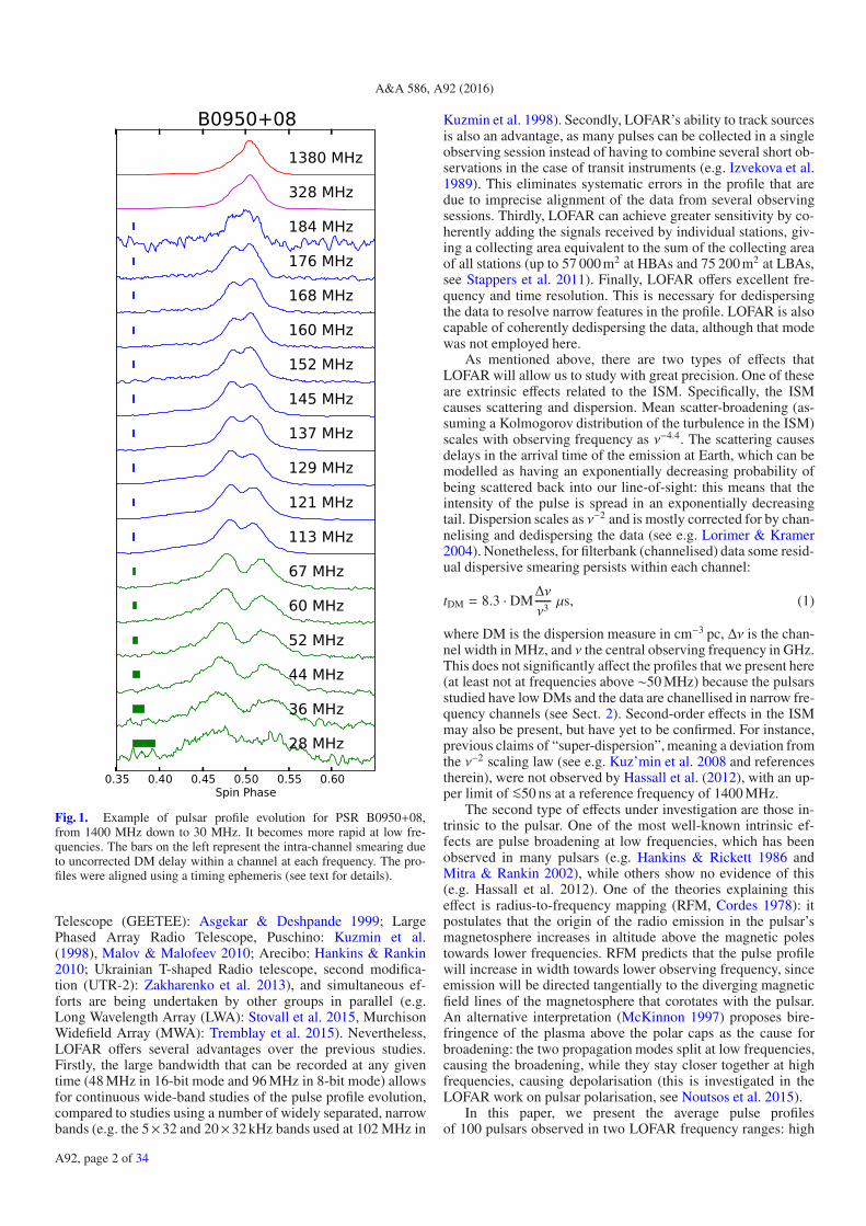
Fig. 7. Distribution of the indices δ of the power law used to computethe evolution of w10 across our frequency range as w10(ν) ∝ νδ.

show RFM and increase their separation with decreasing observ-ing frequency.

Hassall et al. (2012) have discussed that RFM does not seemto be at play for some pulsars observed with LOFAR. Here, witha more statistically significant sample, we can discuss the matterin more detail. Following Thorsett (1991) and in particular Mitra& Rankin (2002), we investigated double-peaked pulse profilesand their component separation (see peak phases in Cols. 5 and 6of Table B.3).

Mitra & Rankin (2002) divided a group of double profile pul-sars into three groups The pulsars from groups A and B are as-sociated with outer cone emission (the difference between thetwo being a fit with or without the constraint ρ0 = ρpc, where ρ0is the constant equivalent to Δθmin from Eq. 11, relative to thebeam radius, and ρpc is the beam radius at the polar cap edge)while the pulsars from group C are associated with inner coneemission. Of the ten pulsars of Mitra & Rankin (2002), the pul-sars from our sample that fall inside each group are

Group A: B0301+19, B0525+21, and B1237+25

Group B: B0329+54 and B1133+16

Group C: B0834+06, B1604−00, and B1919+21.

Mitra & Rankin (2002) reported that pulsars from groups Aand B show RFM, while the pulsars from group C show almostno evolution at all. Although the profile in our sample evolvesrapidly at low frequency, it seems that a similar behaviour canbe observed (see single cases in Fig. B.1).

Figures 3 and 7 show a similar calculation using w10. Weplotted the evolution of w10 as a function of observing fre-quency for the single-peaked pulsars and the histogram of thespectral indices of this evolution. We excluded the LBA andHBA profiles that showed significant scattering. The errors werecalculated from the Gaussian fit, taking into account both thenoise contribution and any unaccounted scattering of the pro-file. Although the values in Fig. 3 seem to follow the power-law,the profile width in some cases effectively behaves in a non-linear way, as can be cross checked in Fig. B.1 for the singlecases.

A92, page 11 of 34

A&A 586, A92 (2016)

The weighted mean spectral index from Fig. 7 is δ = −0.1(2).Our results are compatible at 1σ with the predictions made byBarnard & Arons (1986): the component separation does notvary (no RFM, δ ∼ 0.0), but the distribution in Fig. 7 peaks atnegative spectral indices, which is evidence for a weak widen-ing of the profile at low frequencies. Following the predictions ofGil & Krawczyk (1996), the dependence of w10 with observingfrequency based on their calculations should be δ = −0.21 forRFM and conal beams. This is in support of their model, whilethe fact that we see a broad distribution and a flatter median in-dex might be explained by a subdivision of pulsar behavioursaccording to the Rankin groups. For a future complete analysis,geometry should be taken into account to perform a study on thebeam radii (ρ) rather than the pulse widths.

An alternative but complementary explanation to the ob-served widening of pulsar profiles with decreasing observing fre-quency can be found in the theory of birefringence of two differ-ent propagation modes of a magneto-active plasma (McKinnon1997). These two modes of propagation follow a different pathalong the open field lines. The nature of birefringence is suchthat the two polarisations are spatially closer together at higherfrequencies, and depolarisation will occur where they overlap.Beskin et al. (1988) predicted that the two modes of propagationwould result in two different indices: δ = −0.14 and δ = −0.29for the ordinary mode and δ = −0.5 for the extraordinary mode.While our observations are compatible with either scenario or acombination of them, polarisation studies will help discern be-tween the two interpretations of this phenomenon (see Noutsoset al. 2015).

5.1.2. Profile complexity

Karastergiou & Johnston (2007) searched for a relation betweenthe number of peaks in the profile of a pulsar and some observedor derived parameters, such as its period, age, and rotational en-ergy loss. As a general trend, they found that faster, younger,more energetic pulsars would typically show less complex pro-files, which prompted them to assume that the regions of emis-sion for these pulsars arise at higher altitudes in the magneto-sphere and are, therefore, less numerous (see Sect. 5.1). Notably,an abrupt change in this respect can be observed at P < 150 ms,τ < 105 yr and E > 1035 erg s−1.

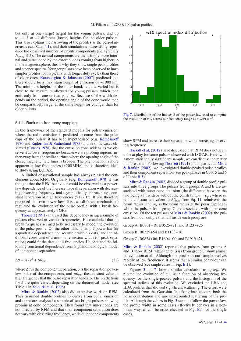
We calculated the same relations using our sampleof 100 pulsars and made the comparisons using LOFAR HBAband and the L-band data. Figure 8 shows the relation betweenthe period of the pulsar and its spin-down age τ for the two fre-quency bands. Each circle represents a pulsar, and its colour anddiameter represent a different number of peaks of its profile. Thecircles are larger for growing number of peaks with frequency,and the number of peaks is ordered by colour, in the order white,red, green, blue, and purple. In the histograms we summed thepulsars separated by number of peaks in their profiles to searchfor trends as a function of either period or τ. No trends are ev-ident in any of the histograms. Our sample does not cover theregion of young energetic pulsars in a statistically significantway so that while the few cases might confirm the predictions ofKarastergiou & Johnston (2007), nothing in favour or disfavourcan be stated in this respect.

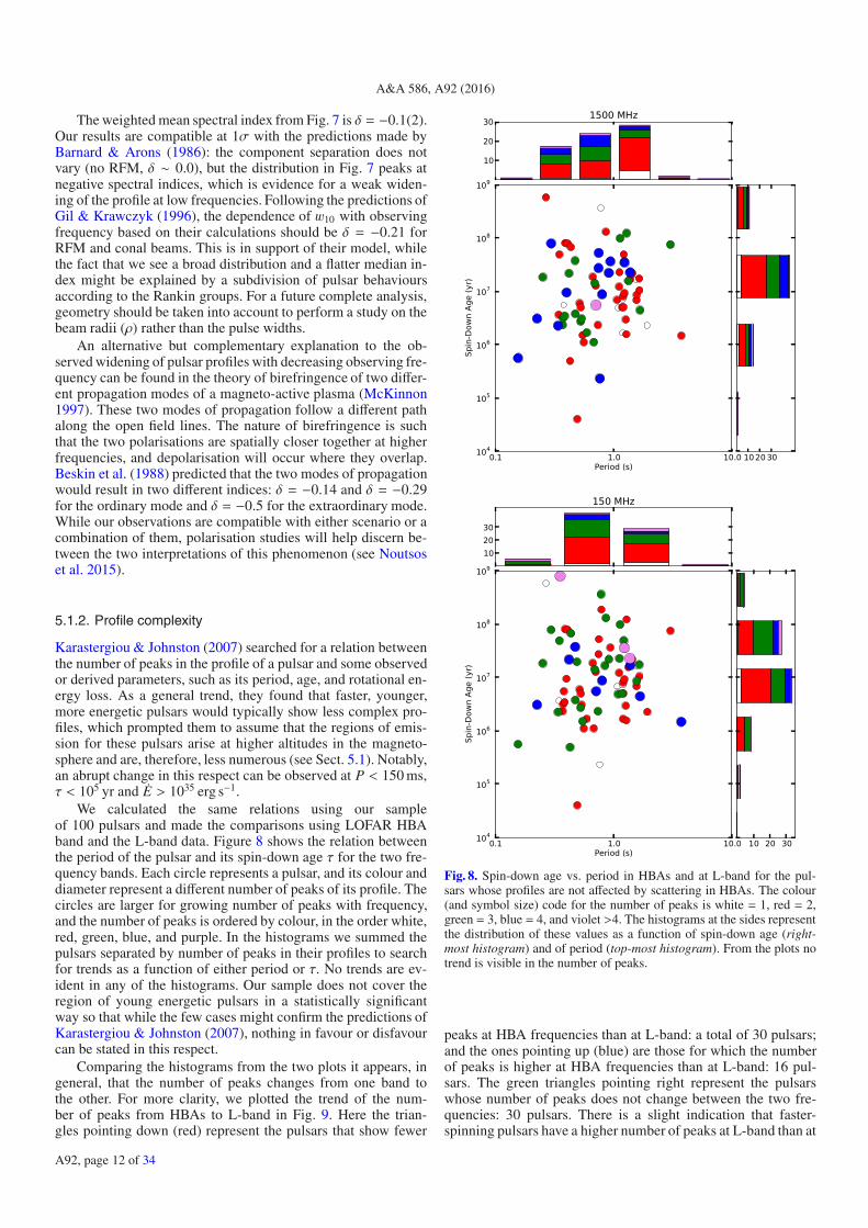
Comparing the histograms from the two plots it appears, ingeneral, that the number of peaks changes from one band tothe other. For more clarity, we plotted the trend of the num-ber of peaks from HBAs to L-band in Fig. 9. Here the trian-gles pointing down (red) represent the pulsars that show fewer

Fig. 8. Spin-down age vs. period in HBAs and at L-band for the pul-sars whose profiles are not affected by scattering in HBAs. The colour(and symbol size) code for the number of peaks is white = 1, red = 2,green = 3, blue = 4, and violet >4. The histograms at the sides representthe distribution of these values as a function of spin-down age (right-most histogram) and of period (top-most histogram). From the plots notrend is visible in the number of peaks.

peaks at HBA frequencies than at L-band: a total of 30 pulsars;and the ones pointing up (blue) are those for which the numberof peaks is higher at HBA frequencies than at L-band: 16 pul-sars. The green triangles pointing right represent the pulsarswhose number of peaks does not change between the two fre-quencies: 30 pulsars. There is a slight indication that faster-spinning pulsars have a higher number of peaks at L-band than at

A92, page 12 of 34

M. Pilia et al.: LOFAR 100 pulsar profiles

Fig. 9. Spin-down age vs period for the pulsars whose profiles are notaffected by scattering in HBAs. Here the shape- and colour-coding rep-resent the difference of the number of peaks for each pulsar betweenHBAs and L-band relative to the HBAs. In red (triangles down) are thepulsars for which the number of peaks becomes smaller at HBAs thanit is in L-band, in blue (triangles up) are the pulsars for which the num-ber of peaks becomes higher at HBAs than it is in L-band, and in green(triangles right) are the pulsars for which the number of peaks does notchange. At the top and on the right-hand side the stacked histogramsrepresent the trends of the number of peaks as a function of period andage of the pulsar, respectively.

HBA frequencies while the slower spinners have more peaks atHBA frequencies than at L-band. The younger pulsars in gen-eral have more peaks at L-band than HBAs; the older havefewer peaks at L-band than at HBAs. In both cases the nullhypothesis probability that the two distributions are the samebased on the Kolmogorov-Smirnoff statistics cannot be rejectedat the 20% confidence level. This, as pointed out by Lyne &Manchester (1988), might be a selection effect or a resolutioneffect (as fast pulsars tend to have wider pulses that can be re-solved more easily), but given our statistics, we can also ten-tatively assume that our sample includes pulsars with differentbehaviours.

Additionally, a number of pulsars show an increase in thenumber of components at HBA compared to L-band, which mayalso be explained at HBA frequencies by the general expectationthat a higher portion of the beam can come into view at lowerfrequencies, according to RFM. On the other hand, the fastestand youngest pulsars show an opposite trend, similar to what isalso observed in millisecond pulsars (see Kondratiev et al. 2016),which are even faster and therefore have a wider duty-cycle (seeFig. 5). A similar finding was also reported by Hankins & Rickett(1986), who analysed the frequency dependence of pulsar pro-files for 12 pulsars in the 135–2380 MHz frequency range. Theyargued that the occurrence of single profiles at low frequenciesthat become multiple at high frequencies can be explained in theframework of the “core and cones” models (in the formulationof Rankin 1993). In particular, this is expected to occur if we canonly observe the core emission at low frequencies, which is ob-served to typically have a steeper spectrum, while the outriding

conal components only emerge at higher observing frequency(see Kramer et al. 1994 for arguments why this is caused bygeometrical reasons and applies to inner and outer componentsregardless of their “nature” as core or cones). A word of cau-tion is needed here, related to how the number of peaks wasdetermined: it is possible that we achieved a good fit to the pro-file using a smaller number of Gaussians in HBAs relative toL-band because the quality of the profile is lower and so fewercomponents need be fit (for details on the method see Sect. 3,and the single cases can be studied by comparing Fig. B.1 andTable B.2).

5.2. External effects on profile evolution

The interstellar medium affects the pulse signal while it trav-els towards the observer, and it strongly depends on observ-ing frequency, with observations at low frequencies being morestrongly affected by scattering and dispersion delay (see alsoZakharenko et al. 2013). We here did not correct the profiles pre-sented for scattering effects that can smear out the signal espe-cially at LBA frequencies, but we considered the effect of intra-channel dispersive smearing.

The DM represents the integrated column density of freeelectrons between the pulsar and the observer. It produces a timedelay in the signal, between the observing frequency and infinitefrequency, that can be approximated as

ΔtDM =[ DM

cm−3pc ]

2.41 × 10−4[ νMHz ]2

s. (12)

This approximation is valid if the plasma is tenuous and thuscollisionless and if the observing frequency is much greater thanthe plasma frequency and the electron gyrofrequency. Signalsat different frequencies will be delayed, with the lowest fre-quencies being delayed the most. These delays can change ontimescales of some years, up to 10−3 cm−3 pc (see e.g. Keith et al.2013).

When aligning the profiles absolutely as we did, connect-ing the reference point of the profile to the reference epoch ofthe ephemeris, the DM delays had to be taken into account andall reference times converted to the corresponding times at infi-nite frequency to correct for dispersive delay. Hankins & Rickett(1986) described a way to measure DM variations based on thealignment of pulsar profiles at different frequencies. Hankinset al. (1991) and Hankins & Rankin (2010) followed this methodusing increasingly higher resolution profiles. They absolutelyaligned the profiles spanning, where possible, all the octavesof radio frequency. Leaving the DM as the only free parame-ter, they identified a reference point in the profile and adjustedthe DM value to compensate for the remaining misalignment ofthe profiles. The value of the best DM was obtained this way, itsaccuracy strongly depending on the lower frequency that can beused and on the precision with which the time difference of themisalignment can be measured.

All the pulsars from our sample were aligned by refold-ing their profiles at all frequencies using the same ephemeris.The DM that was adopted for the alignment was the one ob-tained from LOFAR HBA data: a first folding was performedwith prepfold using the new ephemeris created from the Lovelldata (see Sect. 3), but allowing for a search over DM values,and then the best DM obtained from this search was includedin the ephemeris and the profile was dedeispersed once more,without any search option. The same was done for the LBA

A92, page 13 of 34

A&A 586, A92 (2016)

and the P- and L-band observations. Figure B1 shows that themulti-frequency profiles are aligned in most cases. There weresome cases, discussed in Sect. 3, where the alignment is visi-bly incorrect or where we had to apply an extra adjustment toDM to compensate for a visible offset between the profiles (seeTable 1).

One possible cause for the misalignment is the evolution ofthe profile across the frequencies, so that it is not possible toeasily identify a fiducial point in the profile. In addition, pul-sars strongly affected by scattering will not only have an ex-ponential scattering tail, but also an absolute delay. Our profilealignment seemed to also be affected by the significantly dif-ferent observing epochs (e.g. the WSRT observations were per-formed more than ten years before LOFAR observations). Onone hand, this meant that we had to adopt a timing solutionspanning a long period of time, where timing noise and othereffects can become substantial. On the other hand, with observa-tions so far apart, we might also be probing gradients in electrondensity.

In our case it is not yet possible to perform a systematicstudy of these variations, as was done by Keith et al. (2013).Nonetheless, LOFAR data can provide a new wealth of DM mea-surements to be compared with previous observations to map theevolution of the interstellar dispersion with time. A first conclu-sion that can be drawn from this, simply by comparing the DMvalues in Table B.1, is that there is no significant indication ofDMs being systematically higher at low frequencies (at least atour measurement precision). Some authors (e.g. Shitov 1983)have postulated “superdispersion” due to the sweepback of fieldlines in the pulsar magnetosphere, which would be responsiblefor lower dispersion delays at low frequencies and could createan observed profile misalignment over a wide observing band.We find that the ratio DMHBA/DMeph ranges from 0.97 to 1.06(see Table B.1), thus differing by a significant percentage insome cases, but in both directions, thus not favouring superdis-persion. This agrees with previous findings using LOFAR data(Hassall et al. 2012) and previous measurements (Hankins et al.1991).

5.3. Some examples of unexpected profile evolution

It is not in the scope of this initial paper to enter into much detailabout the profile evolution of specific pulsars. These will be thesubject of future dedicated work. There are, however, several in-teresting cases of pulse evolution that are worth pointing out atthis time.

Figures 3 and 7 showed that there are some cases (e.g.B1541+09, B1821+05, and B1822–09, B2224+65) where thewidth of the profile is observed to increase with increasing ob-serving frequency. If we compare these results with the singleprofiles in Fig. B.1, we notice that in these cases this is causedby new peaks appearing in the profile at higher frequencies (e.g.the well-known “precursor” in the case of B1822–09). This isnot common in the standard core and cones geometries, eventhough it is predicted that new components can come into viewif our viewing angle changes with increasing observing fre-quency, thus allowing us to see deeper into the beam. Whilethis would explain some of the cases, in some others the pro-file evolution can hardly be ascribed to a symmetric core andconal structure (see e.g. B0355+54, B0450+55, B1831–04, andB1857–26).

These narrowing profiles at low frequencies might be inter-preted as evidence for fan beam models (Michel 1987). In fan

beam models by Dyks et al. (2010), Dyks & Rudak (2012, 2015),for instance, the emission comes from elongated broad-bandstreams that follow the magnetic field lines. The model, based onthe cut angle at which the line of sight crosses the beam, can ex-plain the lack of RFM, for example, if the stream is very narrow(also the case for millisecond pulsars), and it can also explainthe “inverse” RFM if there is spectral non-uniformity along theazimuthal direction of the beam through which our line of sightcuts. The fan-beam formulation proposed by Wang et al. (2014)can even explain “regular” RFM by assuming that a fan beamcomposed of a (small) number of sub-beams will produce a so-called “limb-darkening pattern” that is caused by the decreasein intensity with beam radius of the emission at higher altitudesbecause the emission is farther from the magnetic pole. Theirmodel, based on observations and simulations, predicts that thenon-circularly bound beam (different in this from the beam pre-dicted by the narrow-band models) can depart from the relationw ∝ P−1/2 (where w is the measured width of the profile, seeSect. 4.1).

Chen & Wang (2014), who recently analysed the pulse widthevolution with frequency of 150 pulsars from the EPN database,reached a similar conclusion: the emission must be broad-band,and the observed behaviour of width at different frequenciesis caused by spectral changes along the flux tube. They foundthat if the spectral index variation along pulse phase is sym-metric, there can be either canonical RFM or anti-RFM, whilein cases where there are substantial deviations from the sym-metric case, then there can be the non-monotonic trends of w10with ν, which we also observed. This is supported theoreticallyby the particle-in-cell simulations of pair production in the vac-uum gaps (Timokhin 2010), which predict that the secondaryplasma does not necessarily have a monotonic momentumspectrum.

These results, and in particular the fact that a wide stream isexpected to produce spectral variations longitudinally in the pro-files, could also explain the observed behaviour of the peak ratiosshown in Fig. 6. Alternatively, the peak ratio changing with ob-serving frequency and, in particular, its changing sign, might berelated to the frequency dependance of the two modes of polari-sation (ordinary, “O”, and extraordinary, “X”) (e.g., Smits et al.2006) and to that they might be differently dominant in differentpeaks. While it is not possible to give a comprehensive analysisof the phenomenon here, our studies on the polarised emissionfrom pulsars with LOFAR (see Noutsos et al. 2015) address thequestions related to the orthogonally polarised modes and therelated jumps in the polarisation angle.

While in this section we have discussed some unexpectedprofile evolution, it remains the case that most pulsar profiles(cf. Sects. 4.1 and 5.1.1) are well described by RFM.

6. Summary and future work

We have presented the profiles of the first 100 pulsars observedby LOFAR in the frequency range 119–167 MHz. Twenty-six ofthem were also detected with 57 min integrations using LOFARin the interval 15–63 MHz. All the LOFAR profiles presented inthis work will be made available through the EPN database10.LOFAR observations were compared with archival WSRT orLovell observations in P- and L-band, after first folding andaligning all profiles using an ephemeris spanning the full rangeof the observations. The rotational and derived parameters are

10 http://www.epta.eu.org/epndb/

A92, page 14 of 34

M. Pilia et al.: LOFAR 100 pulsar profiles

presented in Table B.1. Two values of DM were presented aswell: one obtained by the best timing fit and one from the best fitof LOFAR data. For each pulsar we aligned the profiles at dif-ferent frequencies in absolute phase, using the latter DM value.The 100 profiles are presented in Fig. B.1.

Each profile of every pulsar was described using a multi-Gaussian fit following the approach of Kramer et al. (1994),so that in general more components were needed to fit the pro-files than evident at first glance or traditionally considered (e.g.Rankin 1983b). The results of the Gaussian fit (the measure-ment of the widths at half and at 10% of the maximum of theprofile and the spectral index of their evolution with observingfrequency) are reported in Table B.2. Using the components’widths, we calculated the ratio of the peaks for pulsars with dou-ble or multiple peaks (the two most prominent, in the case ofmultiple peaks pulsars). We concluded that the ratio of the mainpeak to the second peak does not follow a unique trend, althoughwe note that in most cases the dominant peak alternates withchanging observing frequency. Using w10 , we followed the evo-lution of the width of the full profile with observing frequency.We concluded that while our average spectral index is compati-ble with no evolution of the pulse width, the distribution of thevalues is quite large and compatible with the presence of differ-ent behaviours for different pulsars, for example, based on inneror outer cone emission, as discussed by Mitra & Rankin (2002),or on different propagation modes in the magnetosphere (e.g.Beskin et al. 1988; Beskin & Philippov 2012).

Future work will be needed, and is in progress, to add moreelements to complete this puzzle. Parallel to this work, a similarone is being conducted on the evolution of the profiles of mil-lisecond pulsars at low frequencies (Kondratiev et al. 2016), andthe spectral behaviour of the slow and recycled pulsars has beenanalysed (Hassall et al., in prep.). Complementary to our workis the study of the polarisation properties of pulsars (Noutsoset al. 2015): the study of the polarisation properties can giveconstraints on the geometry of the pulsar emission and there-fore on its height and on the intrinsic opening angle of thebeam of the emission. Additionally, polarisation can help distin-guish between orthogonal polarisation modes and therefore de-termine whether the observed widening of the profiles is causedby birefringence.

To better constrain the width of the pulse, it is also importantto be able to deconvolve the scattering tail, which in some casesbecomes dominant at low frequencies, from the intrinsic widthof the profile. Studies on the characterisation of scattering at lowfrequencies and modelling of the scattering tail are being con-ducted (Archibald et al. 2014, Zagkouris et al. in prep.). At thesame time, the effects of the ISM on LOFAR profiles are beingused to create an “ISM weather” database, where the DM vari-ations, independently measured with LOFAR (Verbiest et al., inprep.), can be used for high-precision timing measurements frompulsar timing arrays (see Keith et al. 2013).

Finally, the observations presented in this work were fromcommissioning LOFAR data; as mentioned, LOFAR is currentlyperforming the LOTAAS all-sky pulsar survey. When com-pleted, it will provide an extraordinary database of 1.5 h cover-age of the whole northern sky with 0.49 ms time resolution anddown to a flux S min ∼ 6 mJy at 135 MHz. At present we are ableto use the full LOFAR core instead of only the “Superterp” andcan cover a full 80 MHz bandwidth contiguously. Moreover, fur-ther improvements will include coherent dedispersion of the dataand will enable single pulse studies to probe the “instantaneous”magnetosphere.

Acknowledgements. M.P. wishes to thank A. Archibald, V. Beskin and J. Dyksfor useful discussion. We are grateful to an anonymous referee whose com-ments notably improved the quality of our work. This work was made possi-ble by an NWO Dynamisering grant to ASTRON, with additional contributionsfrom European Commission grant FP7-PEOPLE-2007-4-3-IRG-224838 to JVL.LOFAR, the Low-Frequency Array designed and constructed by ASTRON, hasfacilities in several countries, that are owned by various parties (each with theirown funding sources), and that are collectively operated by the InternationalLOFAR Telescope (ILT) foundation under a joint scientific policy. M.P. ac-knowledges financial support from the RAS, Autonomous Region of Sardinia.J.W.T.H., V.I.K. and J.V.L. acknowledge support from the European ResearchCouncil under the European Union’s Seventh Framework Programme (FP/2007-2013) / ERC Grant Agreement nrs. 337062 (JWTH, VIK) and 617199 (JVL). SOis supported by the Alexander von Humboldt Foundation. C. Ferrari acknowl-edges financial support by the “Agence Nationale de la Recherche” through grantANR-09-JCJC-0001-01.

ReferencesAbdo, A. A., Ajello, M., Allafort, A., et al. 2013, ApJS, 208, 17Alexov, A., Hessels, J., Mol, J. D., Stappers, B., & van Leeuwen, J. 2010, in

Astronomical Data Analysis Software and Systems XIX, eds. Y. Mizumoto,K.-I. Morita, & M. Ohishi, ASP Conf. Ser., 434, 193

Archibald, A. M., Kondratiev, V. I., Hessels, J. W. T., & Stinebring, D. R. 2014,ApJ, 790, L22

Arzoumanian, Z., Chernoff, D. F., & Cordes, J. M. 2002, ApJ, 568, 289Asgekar, A., & Deshpande, A. A. 1999, Bull. Astron. Soc. India, 27, 209Barnard, J. J., & Arons, J. 1986, ApJ, 302, 138Beskin, V. S., & Philippov, A. A. 2012, MNRAS, 425, 814Beskin, V. S., Gurevich, A. V., & Istomin, I. N. 1988, Ap&SS, 146, 205Bilous, A. V., Hessels, J. W. T., Kondratiev, V. I., et al. 2014, A&A, 572, A52Camilo, F., & Nice, D. J. 1995, ApJ, 445, 756Chen, J. L., & Wang, H. G. 2014, ApJS, 215, 11Coenen, T., van Leeuwen, J., Hessels, J. W. T., et al. 2014, A&A, 570, A60Cordes, J. M. 1978, ApJ, 222, 1006Cordes, J. M. 1993, in Planets Around Pulsars, eds. J. A. Phillips, S. E. Thorsett,

& S. R. Kulkarni, ASP Conf. Ser., 36, 43Dyks, J., & Rudak, B. 2012, MNRAS, 420, 3403Dyks, J., & Rudak, B. 2015, MNRAS, 446, 2505Dyks, J., Rudak, B., & Demorest, P. 2010, MNRAS, 401, 1781Espinoza, C. M., Lyne, A. G., Stappers, B. W., & Kramer, M. 2011, MNRAS,

414, 1679Espinoza, C. M., Lyne, A. G., Stappers, B. W., & Kramer, M. 2012, VizieR

Online Data Catalog: J/MNRAS/414/41679Gil, J., & Krawczyk, A. 1996, MNRAS, 280, 143Gil, J., Gronkowski, P., & Rudnicki, W. 1984, A&A, 132, 312Gil, J. A., Kijak, J., & Seiradakis, J. H. 1993, A&A, 272, 268Gould, D. M., & Lyne, A. G. 1998, MNRAS, 301, 235Hamilton, P. A., & Lyne, A. G. 1987, MNRAS, 224, 1073Hankins, T. H., & Rankin, J. M. 2010, AJ, 139, 168Hankins, T. H., & Rickett, B. J. 1986, ApJ, 311, 684Hankins, T. H., Izvekova, V. A., Malofeev, V. M., et al. 1991, ApJ, 373, L17Hassall, T. E., Stappers, B. W., Hessels, J. W. T., et al. 2012, A&A, 543, A66Helfand, D. J., Manchester, R. N., & Taylor, J. H. 1975, ApJ, 198, 661Hirotani, K. 2011, ApJ, 733, L49Hobbs, G., Lyne, A. G., Kramer, M., Martin, C. E., & Jordan, C. 2004, MNRAS,

353, 1311Hotan, A. W., van Straten, W., & Manchester, R. N. 2004, PASA, 21, 302Izvekova, V. A., Malofeev, V. M., & Shitov, Y. P. 1989, Sov. Ast., 33, 175Izvekova, V. A., Kuzmin, A. D., Lyne, A. G., Shitov, Y. P., & Smith, F. G. 1993,

MNRAS, 261, 865Janssen, G. H., & Stappers, B. W. 2006, A&A, 457, 611Karastergiou, A., & Johnston, S. 2007, MNRAS, 380, 1678Keith, M. J., Coles, W., Shannon, R. M., et al. 2013, MNRAS, 429, 2161Komesaroff, M. M. 1970, Nature, 225, 612Kondratiev, V. I., Verbiest, J. P. W., Hessels, J. W. T., et al. 2016, A&A, 585,

A128Kramer, M. 1994, A&AS, 107, 527Kramer, M., Wielebinski, R., Jessner, A., Gil, J. A., & Seiradakis, J. H. 1994,

A&AS, 107, 515Kuzmin, A. D., & Losovsky, B. Y. 1999, A&A, 352, 489Kuzmin, A. D., Izvekova, V. A., Shitov, Y. P., et al. 1998, A&AS, 127, 355Kuz’min, A. D., Losovskii, B. Y., Logvinenko, S. V., & Litvinov, I. I. 2008,

Astron. Rep., 52, 910Lewandowski, W., Wolszczan, A., Feiler, G., Konacki, M., & Sołtysinski, T.

2004, ApJ, 600, 905Liu, K., Keane, E. F., Lee, K. J., et al. 2012, MNRAS, 420, 361Lommen, A. N., Zepka, A., Backer, D. C., et al. 2000, ApJ, 545, 1007

A92, page 15 of 34

A&A 586, A92 (2016)

Lorimer, D. R. 2008, Liv. Rev. Relat., 11, 8Lorimer, D. R., & Kramer, M. 2004, Handbook of Pulsar Astronomy

(Cambridge, UK: Cambridge University Press)Lorimer, D. R., Yates, J. A., Lyne, A. G., & Gould, D. M. 1995, MNRAS, 273,

411Lyne, A., Hobbs, G., Kramer, M., Stairs, I., & Stappers, B. 2010, Science, 329,

408Lyne, A. G., & Manchester, R. N. 1988, MNRAS, 234, 477Maciesiak, K., Gil, J., & Ribeiro, V. A. R. M. 2011, MNRAS, 414, 1314Maciesiak, K., Gil, J., & Melikidze, G. 2012, MNRAS, 424, 1762Malov, O. I., & Malofeev, V. M. 2010, Astron. Rep., 54, 210Manchester, R. N., Hobbs, G. B., Teoh, A., & Hobbs, M. 2005, AJ, 129, 1993McKinnon, M. M. 1997, ApJ, 475, 763Michel, F. C. 1987, ApJ, 322, 822Mitra, D., & Rankin, J. M. 2002, ApJ, 577, 322Noutsos, A., Sobey, C., Kondratiev, V. I., et al. 2015, A&A, 576, A62Osłowski, S., van Straten, W., Hobbs, G. B., Bailes, M., & Demorest, P. 2011,

MNRAS, 418, 1258Radhakrishnan, V., & Rankin, J. M. 1990, ApJ, 352, 258Rankin, J. M. 1983a, ApJ, 274, 359Rankin, J. M. 1983b, ApJ, 274, 333Rankin, J. M. 1986, ApJ, 301, 901Rankin, J. M. 1990, ApJ, 352, 247Rankin, J. M. 1993, ApJ, 405, 285Ransom, S. M. 2001, Ph.D. Thesis, Harvard UniversityRathnasree, N., & Rankin, J. M. 1995, ApJ, 452, 814Ruderman, M. A., & Sutherland, P. G. 1975, ApJ, 196, 51Sayer, R. W., Nice, D. J., & Taylor, J. H. 1997, ApJ, 474, 426Shitov, Y. P. 1983, Sov. Ast., 27, 314Smits, J. M., Stappers, B. W., Edwards, R. T., Kuijpers, J., & Ramachandran, R.

2006, A&A, 448, 1139Sobey, C., Young, N. J., Hessels, J. W. T., et al. 2015, MNRAS, 451, 2493Stappers, B. W., Hessels, J. W. T., Alexov, A., et al. 2011, A&A, 530, A80Stovall, K., Ray, P. S., Blythe, J., et al. 2015, ApJ, 808, 156Thorsett, S. E. 1991, ApJ, 377, 263Timokhin, A. N. 2010, MNRAS, 408, 2092Tremblay, S. E., Ord, S. M., Bhat, N. D. R., et al. 2015, PASA, 32, 5van Haarlem, M. P., Wise, M. W., Gunst, A. W., et al. 2013, A&A, 556, A2Wang, H.-G., Han, J.-L., & Qian, G.-J. 2001, Chin. Astron. Astrophys., 25, 73Wang, H. G., Pi, F. P., Zheng, X. P., et al. 2014, ApJ, 789, 73Weisberg, J. M., Romani, R. W., & Taylor, J. H. 1989, ApJ, 347, 1030Weltevrede, P., Edwards, R. T., & Stappers, B. W. 2005, VizieR Online Data

Catalog: J/A&A/445/243Weltevrede, P., Edwards, R. T., & Stappers, B. W. 2006, A&A, 445, 243Weltevrede, P., Stappers, B. W., & Edwards, R. T. 2007, A&A, 469, 607Xilouris, K. M., Kramer, M., Jessner, A., Wielebinski, R., & Timofeev, M. 1996,

A&A, 309, 481You, X. P., Hobbs, G., Coles, W. A., et al. 2007, MNRAS, 378, 493Yuan, J. P., Wang, N., Manchester, R. N., & Liu, Z. Y. 2010, MNRAS, 404, 289Zakharenko, V. V., Vasylieva, I. Y., Konovalenko, A. A., et al. 2013, MNRAS,

431, 3624

1 ASTRON, The Netherlands Institute for Radio Astronomy,Postbus 2, 7990 AA Dwingeloo, The Netherlandse-mail: pilia@astron.nl

2 INAF–Osservatorio Astronomico di Cagliari, via della Scienza 5,09047 Selargius (CA), Italy

3 Anton Pannekoek Institute, University of Amsterdam, Postbus94249, 1090 GE Amsterdam, The Netherlands

4 Jodrell Bank Center for Astrophysics, School of Physics andAstronomy, The University of Manchester, Manchester M13 9PL,UK

5 Astro Space Center of the Lebedev Physical Institute,Profsoyuznaya str. 84/32, 117997 Moscow, Russia

6 Max-Planck-Institut für Radioastronomie, Auf dem Hügel 69,53121 Bonn, Germany

7 Astrophysics, University of Oxford, Denys Wilkinson Building,Keble Road, Oxford OX1 3RH, UK

8 School of Physics and Astronomy, University of Southampton,Southampton, SO17 1BJ, UK

9 Department of Astrophysics/IMAPP, Radboud UniversityNijmegen, PO Box 9010, 6500 GL Nijmegen, The Netherlands

10 LPC2E – Universite d’Orleans/CNRS11 Station de Radioastronomie de Nançay, Observatoire de Paris –

CNRS/INSU, USR 704 – Univ. Orléans, OSUC , route de Souesmes,18330 Nançay, France

12 Centre for Astrophysics and Supercomputing, Swinburne Universityof Technology, Mail H29, PO Box 218, VIC 3122, Australia

13 ARC Centre of Excellence for All-sky astrophysics (CAASTRO),Sydney Institute of Astronomy, University of Sydney, Australia

14 NAOJ Chile Observatory, National Astronomical Observatory ofJapan, 2-21-1 Osawa, Mitaka, 181-8588 Tokyo, Japan

15 Fakultät für Physik, Universität Bielefeld, Postfach 100131, 33501Bielefeld, Germany

16 Department of Physics & Astronomy, University of the WesternCape, Private Bag X17, 7535 Bellville, South Africa

17 Space Telescope Science Institute, 3700 San Martin Drive,Baltimore, MD 21218, USA

18 Helmholtz-Zentrum Potsdam, DeutschesGeoForschungsZentrumGFZ, Department 1: Geodesy and Remote Sensing, Telegrafenberg,A17, 14473 Potsdam, Germany

19 Shell Technology Center, 3333 Bangalore, India20 SRON Netherlands Insitute for Space Research, PO Box 800, 9700

AV Groningen, The Netherlands21 Kapteyn Astronomical Institute, PO Box 800, 9700 AV Groningen,

The Netherlands22 CSIRO Australia Telescope National Facility, PO Box 76, Epping

NSW 1710, Australia23 University of Twente, 7522 Enschede, The Netherlands24 Harvard-Smithsonian Center for Astrophysics, 60 Garden Street,

Cambridge, MA 02138, USA25 Leiden Observatory, Leiden University, PO Box 9513, 2300

RA Leiden, The Netherlands26 University of Hamburg, Gojenbergsweg 112, 21029 Hamburg,

Germany27 Leibniz-Institut für Astrophysik Potsdam (AIP), An der Sternwarte

16, 14482 Potsdam, Germany28 Max Planck Institute for Astrophysics, Karl Schwarzschild Str. 1,

85741 Garching, Germany29 Laboratoire AIM (CEA/IRFU – CNRS/INSU – Université Paris

Diderot), CEA DSM/IRFU/SAp, 91191 Gif-sur-Yvette, France30 SmarterVision BV, Oostersingel 5, 9401 JX Assen, The Netherland31 Thüringer Landessternwarte, Sternwarte 5, 07778 Tautenburg,

Germany32 Laboratoire Lagrange, UMR 7293, Université de Nice Sophia-

Antipolis, CNRS, Observatoire de la Côte d’Azur, 06300 Nice,France

33 Astronomisches Institut der Ruhr-Universität Bochum,Universitaetsstrasse 150, 44780 Bochum, Germany

34 Sodankylä Geophysical Observatory, University of Oulu,Tähteläntie 62, 99600 Sodankylä, Finland

35 STFC Rutherford Appleton Laboratory, Harwell Science andInnovation Campus, Didcot OX11 0QX, UK

36 International Centre for Radio Astronomy Research – CurtinUniversity, GPO Box U1987, Perth, WA 6845, Australia

37 Center for Information Technology (CIT), University of Groningen,9700 CA Groningen, The Netherlands

38 Centre de Recherche Astrophysique de Lyon, Observatoire de Lyon,9 avenue Charles André, 69561 Saint-Genis-Laval Cedex, France

39 Department of Physics and Elelctronics, Rhodes University, PO Box94, 6140 Grahamstown, South Africa

40 SKA South Africa, 3rd Floor, The Park, Park Road, 7405 Pinelands,South Africa

41 Department of Astrophysical Sciences, Princeton University,Princeton, NJ 08544, USA

42 LESIA, Observatoire de Paris, CNRS, UPMC, Université Paris-Diderot, 5 place Jules Janssen, 92195 Meudon, France

A92, page 16 of 34

M. Pilia et al.: LOFAR 100 pulsar profiles

Appendix A: Determination of pulse widths

Fig. A.1. PSR B1112+50: example of how the widths of the full profile were calculated using the four methods described in the text. On the left-handside is the real profile. On the right-hand side, for comparison, the noise-free profile obtained from the Gaussian fit. In panel a), the shaded cyanarea represents weff . The dashed vertical lines represent wpow, calculated as shown in panel b): the cumulative distribution of the normalised profile.The solid line demarcates w10 as obtained from the Gaussian smoothed profiles (which are shown in panel a), on the right). The measurement ofw10 is consistent and overlapping with wop (see text for details).

As discussed in the Sects. 3 and 4.1, the widths of the fullprofile that are to be used in the subsequent calculations weredetermined from the fit of Gaussian components to the pro-file shape. However, a number of alternative methods were alsotested and, in one case, used to cross check the widths obtainedfrom the Gaussian fits. Here we give a brief description of eachof them.

We calculated the effective width, weff , as the integratedpulsed flux divided by the peak flux; this is represented bythe cyan-shaded areas in Fig. A.1 centred at the main peak.This width metric typically does not represent all the profilecomponents well, as is observed in the P- and L-band pro-files. The method underestimates the width of the profile formulti-peaked profiles, which is the majority of profiles in thiswork, mainly characterising the width of the main peak in thesecases.

The total-power width wpow is calculated as the phaseinterval that includes 90% of the total pulse energy in thecumulative flux distribution of the normalised profile (see lowerplots in Fig. A.1). We selected the phase included in the intervalbetween 5% of the total flux and 95% of the total flux (indicatedby the intersection of the summed profile with the horizon-tal lines in panel b of Fig. A.1). This distribution should start at 0

and increase monotomically to 1 if no noise is present (see thenoise-free distribution on the right side of Fig. A.1). When noiseis present (left-hand side of Fig. A.1), the sum does not growsmoothly, and sometimes negative terms in the off-pulse regionadd up quite substantially. In the real profiles (left-hand side ofFig. A.1), the horizontal lines should all overlap at 0.05 and 0.95,like they do in the case of the noise-free profiles (right-hand sideof Fig. A.1), but they differ in some cases as they take into ac-count that the highest and lowest value of a noisy cumulativedistribution can be negative or greater than 1. As can be seenfrom the green (LBA) and magenta (P-band) curves, when theprofile is noisier, this measurement is less stable because the cu-mulative distribution oscillates more, and the width can be con-sistently overestimated (in these cases the left-hand dashed lineprecedes the phase range shown in the Fig.). This method is rep-resented by the dotted line in the upper plot of Fig. A.1, which,in the case of the LBA and P-band profiles, starts at phase 0.

The full-width at 10% of the maximum, wop, represents thewidth of the full profile (including noise) at the 10% level of theouter components, including the full on-pulse region: it is coin-cident with the solid vertical lines in Fig. A.1. It was calculatedas the on-pulse region with a flux above 10% of the main peakin the baseline-subtracted profile.

A92, page 17 of 34

A&A 586, A92 (2016)

Appendix B: Multi-frequency profiles and tables of the derived profile properties.

Fig. B.1. Pulse profiles of the 100 pulsars observed by LOFAR, showing from bottom to top LBA (green) and HBA (blue) profiles from LOFARobservations, 350 MHz (magenta) and 1400 MHz (red) profiles from WSRT and Lovell observations. We caution that the moding pulsars, forwhich only one mode of pulsation is represented by our observation, might not be the same for the profiles at different frequencies. The profilephase is zoomed-in on the interval 0.25–0.75 in all cases except for the pulsars with interpulses, where the full pulse phase is shown, and theprofile is rotated by 0.25 in phase to shift the interpulse from phase 0. The star next to the band name indicates that the alignment for that bandwas made manually (see text for details).

A92, page 18 of 34

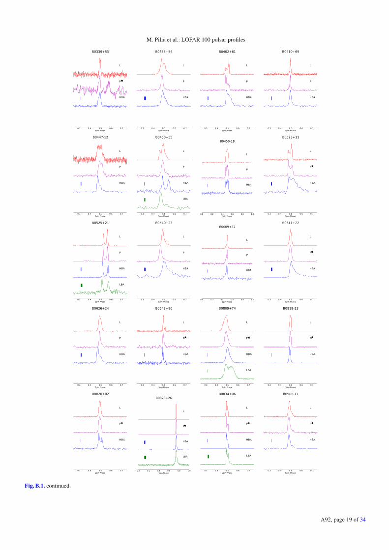
M. Pilia et al.: LOFAR 100 pulsar profiles

Fig. B.1. continued.

A92, page 19 of 34

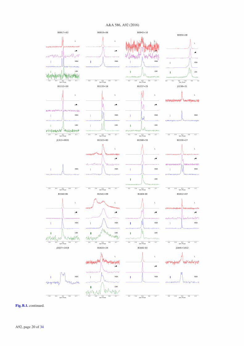
A&A 586, A92 (2016)

Fig. B.1. continued.

A92, page 20 of 34

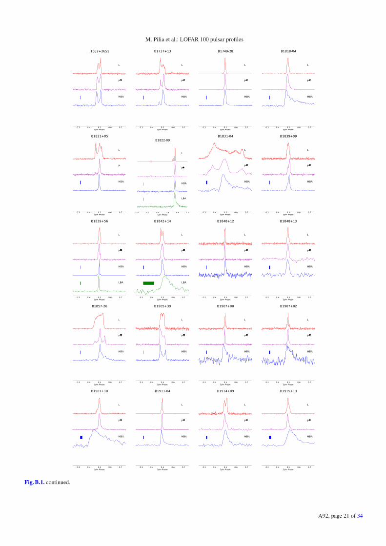
M. Pilia et al.: LOFAR 100 pulsar profiles

Fig. B.1. continued.

A92, page 21 of 34

A&A 586, A92 (2016)

Fig. B.1. continued.

A92, page 22 of 34

M. Pilia et al.: LOFAR 100 pulsar profiles

Fig. B.1. continued.

Fig. B.2. Zoom-in on the 0.0−0.5 phase longitude of the profile for the five pulsars in our sample that have interpulses. The plots are scaled so thateach profile has the same rms and are renormalised to the peak of the interpulse at each frequency. In all cases LBA profiles were removed, astheir signal-to-noise ratio and their channel smearing did not enable any estimate of the interpulse. The reference phase of the main pulse has beenshifted by 0.75, relative to the main plots, to place the interpulse at the centre of the plot.

A92, page 23 of 34

A&A 586, A92 (2016)Ta

ble

B.1

.Lis

tof

the

100

puls

ars

and

thei

rro

tati

onal

and

deri

ved

para

met

ers.

PS

RN

ame

PP

Epo

chL

BA

Epo

chH

BA

Epo

chD

Mep

hD

MH

BA

logτ

log

Blo

gE

Not

es[s

][s

s−1]

[MJD

][M

JD]

[MJD

][c

m−3

pc]

[cm−3

pc]

[yr]

[G]

[s−1

erg]

B00

11+

471.

241

5.64

7e-1

655

316

5585

830

.67(

7)[1

]30

.3(5

)7.

5411.9

331.0

7W

ES

d

B00

31−0

70.

943

4.08

1e-1

655

857

5663

011

.28(

8)[1

]10

.9(4

)7.

5611.8

031.2

8W

ES

d

J005

1+04

230.

355

7.04

7e-1

849

800

5631

813

.9(1

)[2]

13.9

3(1)

8.90

10.7

030.7

9L

OTA

AS

b

B00

59+

651.

679

5.97

0e-1

556

475

5585

965

.85(

2)[1

]65

.8(8

)6.

6512.5

131.7

0E

PN

d

B01

05+

651.

284

1.29

2e-1

454

578

5585

930

.6(5

)[1]

30.6

(2)

6.20

12.6

232.3

8P

-20

04c

B01

14+

580.

101

5.84

6e-1

555

829

5585

949

.462

(4)[1

]49

.42(

1)5.

4411.8

935.3

4E

PN

d

B01

36+

570.

272

1.06

9e-1

454

589

5585

973

.776

(6)[1

]73

.83(

1)5.

6112.2

434.3

2P

-,L

-20

04b

B01

38+

591.

223

3.91

0e-1

654

266

5592

455

859

34.7

4(1)

[1]

34.9

2(2)

7.70

11.8

430.9

3P

-20

04c

B03

01+

191.

388

1.29

5e-1

555

743

5585

915

.851

(9)[1

]15

.65(

4)7.

2312.1

331.2

8W

ES

d

B03

20+

393.

032

6.35

8e-1

654

125

5592

455

859

25.9

9(3)

[1]

26.1

9(1)

7.88

12.1

529.9

5P

-20

02c

B03

29+

540.

715

2.04

6e-1

553

850

5585

955

859

26.7

941(

1)[3

]26

.765

3(<

1)6.

7412.0

932.3

5P

-20

00c

B03

31+

450.

269

7.33

1e-1

855

899

5585

947

.149

(3)[1

]47

.15(

1)8.

7610.6

531.1

7E

PN

d

B03

39+

531.

934

1.34

2e-1

455

804

5585

967

.28(

6)[1

]67

.5(2

)6.

3612.7

131.8

6W

ES

d

B03

55+

540.

156

4.39

5e-1

553

813

5585

957

.122

6(3)

[4]

57.1

4(1)

5.75

11.9

234.6

6P

-20

03c

B04

02+

610.

595

5.57

6e-1

556

097

5585

965

.303

(7)[1

]65

.39(

3)6.

2312.2

733.0

2B

0410+

690.

391

7.65

6e-1

754

418

5585

927

.471

(4)[1

]27

.44(

1)7.

9111.2

431.7

0P

-20

04c

B04

47−1

20.

438

1.02

8e-1

655

203

5656

837

.04(

1)[1

]37

.01(

1)7.

8311.3

331.6

8P

-20

03c

B04

50+

550.

341

2.37

7e-1

554

139

5592

455

861

14.4

83(7

)[1]

14.5

9(7)

6.36

11.9

633.3

8P

-,L

-20

04c

B04

50−1

80.

549

5.75

5e-1

555

203

5660

339

.903

(3)[1

]39

.91(

2)6.

1812.2

533.1

4P

-20

04c

B05

23+

110.

354

7.36

2e-1

755

202

5656

879

.423

(3)[1

]79

.43(

4)7.

8811.2

131.8

1P

-20

06c

B05

25+

213.

746

4.00

4e-1

454

457

5592

456

596

50.9

6(2)

[1]

50.8

7(2)

6.17

13.0

931.4

8P

-20

03,L

-20

04c

B05

40+

230.

246

1.54

2e-1

454

748

5585

977

.631

(2)[1

]77

.7(9

)5.

4012.2

934.6

1P

-20

06c

B06

09+

370.

298

5.98

0e-1

754

590

5585

927

.136

(4)[1

]27

.15(

3)7.

9011.1

331.9

5P

-20

06c

B06

11+

220.

335

5.91

1e-1

455

604

5668

196

.94(

7)[1

]96

.92(

1)4.

9512.6

534.7

9W

ES

d

B06

26+

240.

477

1.98

5e-1

555

071

5585

984

.19(

4)[1

]84

.18(

3)6.

5811.9

932.8

6P

-20

04c

B06

43+

801.

214

3.79

9e-1

554

855

5585

933

.33(

2)[1

]33

.3(1

)6.

7012.3

431.9

2P

-20

04c

B08

09+

741.

292

1.66

0e-1

653

508

5604

655

916

5.73

3(1)

[3]

5.75

(3)

8.09

11.6

730.4

8W

ES

d

B08

18−1

31.

238

2.10

5e-1

555

507

5660

340

.949

(3)[1

]40

.98(

1)6.

9712.2

131.6

4W

ES

d

B08

20+

020.

865

1.04

7e-1

655

508

5630

123

.717

(6)[1

]23

.76(

7)8.

1211.4

830.8

1W

ES

d

B08

23+

260.

531

1.67

9e-1

555

419

5588

955

966

19.4

64(4

)[1]

19.4

711(<

1)6.

7011.9

832.6

5W

ES

d

B08

34+

061.

274

6.79

9e-1

555

507

5588

355

881

12.8

91(6

)[1]

12.8

735(<

1)6.

4712.4

732.1

1W

ES

d

B09

06−1

70.

402

6.69

3e-1

654

887

5660

315

.885

(3)[1

]15

.87(

1)6.

9811.7

232.6

1W

ES

d

B09

17+

631.

568

3.60

8e-1

553

883

5592

555

860

13.2

1(2)

[1]

13.1

4(2)

6.84

12.3

831.5

7E

PN

d

B09

19+

060.

431

1.37

2e-1

455

870

5631

527

.256

(6)[1

]27

.3(1

)5.

7012.3

933.8

3W

ES

d

Not

es.

(a)

For

each

DM

mea

sure

men

tan

dit

ser

ror

we

quot

eth

ere

fere

nce

pape

r:1,

2,3,

4,5,

6,7,

and

8.(b

)O

bser

vati

ons

from

the

LO

TAA

Ssu

rvey

(Coe

nen

etal

.20

14).

(c)

Yea

rof

the

P-

and/

orL

-ban

dda

tafr

omW

SR

Tob

serv

atio

ns.L

-ban

dda

taw

ere

obta

ined

from

Lov

ell

obse

rvat

ions

inal

lbut

the

thre

eca

ses

whe

reth

eye

arof

the

WS

RT

obse

rvat

ions

isin

dica

ted.

All

the

L-b

and

obse

rvat

ions

usin

gth

eL

ovel

ltel

esco

pew

ere

perf

orm

edbe

twee

nO

ctob

er20

11an

dN

ovem

ber

2013

.(d)

Whe

reP

-ban

dda

taw

ere

avai

labl

efr

omW

elte

vred

eet

al.(

2005

),bu

tno

abso

lute

refe

renc

ew

asav

aila

ble

toal

ign

the

data

wit

hL

OFA

Rda

ta,r

efer

ence

ism

ade

toth

eir

pape

ras

WE

San

dth

eco

rres

pond

ing

profi

lein

Fig

.B.1

was

alig

ned

byey

e.Fo

rco

mpl

eten

ess,

whe

reth

epu

lsar

was

not

inW

ES

,the

nE

PN

indi

cate

sth

atth

epr

ofile

inP

-ban

dw

asob

tain

edfr

omth

eE

PN

puls

arda

taba

sean

dw

asal

soon

lyal

igne

dby

eye.

Inth

isla

tter

case

,the

obse

rvat

ions

are

not

late

rth

an20

02.I

nth

eca

ses

whe

reno

thin

gis

spec

ified

,for

the

P-b

and

the

profi

leis

eith

erm

issi

ngin

all

the

data

base

sus

edhe

reor

the

Lov

ell

data

wer

eus

edan

dth

epr

ofile

alig

ned

wit

hth

est

anda

rdpr

oced

ure

asde

scri

bed

inth

ete

xt.

Ref

eren

ces.

(1)

Hob

bset

al.(

2004

);(2

)S

ayer

etal

.(19

97);

(3)

Has

sall

etal

.(20

12);

(4)

Jans

sen

&S

tapp

ers

(200

6);(

5)L

omm

enet

al.(

2000

);(6

)L

ewan

dow

skie

tal.

(200

4);(

7)H

amil

ton

&L

yne

(198

7);(

8)C

amil

o&

Nic

e(1

995)

.

A92, page 24 of 34

M. Pilia et al.: LOFAR 100 pulsar profiles

Tabl

eB

.1.c

onti

nued

.

PS

RN

ame

PP

Epo

chL

BA

Epo

chH

BA

Epo

chD

Mep

hD

MH

BA

logτ

log

Blo

gE

Not

es[s

][s

s−1]

[MJD

][M

JD]

[MJD

][c

m−3

pc]

[cm−3

pc]

[yr]

[G]

[s−1

erg]

B09

43+

101.

098

3.54

6e-1

554

226

5592

555

869

15.2

(5)[1

]15

.32(

1)6.

6912.3

032.0

2E

PN

d

B09

50+

080.

253

2.16

5e-1

651

541

5588

956

603

2.96

1(3)

[1]

2.96

96(<

1)7.

2711.3

732.7

2E

PN

d

B11

12+

501.

656

2.49

3e-1

554

121

5592

556

233

9.20

2(8)

[1]

9.18

(1)

7.02

12.3

131.3

4W

ES

d

B11

33+

161.

188

3.73

3e-1

556

235

5592

555

916

4.86

11(1

)[3]

4.82

62(<

1)6.

7012.3

331.9

4W

ES

d

B12

37+

251.

382

9.59

6e-1

646

498

5592

555

860

9.25

4(6)

[1]

9.25

38(<

1)7.

3612.0

731.1

6W

ES

d

J123

8+21

1.11

91.

445e

-15

5550

755

860

17(2

)[1]

17.9

7(3)

7.09

12.1

131.6

1J1

313+

0931

0.84

98.

000e

-16

5098

455

860

12.0

(1)[5

]12

.05(

2)7.

2311.9

231.7

1B

1322+

830.

670

5.67

5e-1

653

763

5586

013

.3(2

)[1]

13.3

1(3)

7.27

11.8

031.8

7W

ES

d

B15

08+

550.

740

5.00

7e-1

555

168

5590

655

860

19.5

9(2)

[1]

19.6

179(<

1)6.

3712.2

932.6

9W

ES

d

B15

30+

271.

125

7.79

1e-1

656

508

5585

914

.76(

2)[1

]14

.7(2

)7.

3611.9

831.3

3W

ES

d

B15

40−0

60.

709

8.81

0e-1

655

962

5589

256

605

18.4

03(4

)[1]

18.3

788(<

1)7.

1111.9

031.9

9W

ES

d

B15

41+

090.

748

4.32

8e-1

655

508

5589

255

859

35.2

4(3)

[1]

34.9

7(3)

7.44

11.7

631.6

1W

ES

d

B16

04−0

00.

422

3.06

3e-1

654

696

5589

256

346

10.6

87(5

)[1]

10.6

9(1)

7.34

11.5

632.2

1W

ES

d

B16

12+

071.

207

2.36

0e-1

555

508

5635

421

.39(

3)[1

]21

.41(

1)6.

9112.2

331.7

2W

ES

d

J162

7+14

190.

491

3.93

0e-1

648

957

5585

933

.8(6

)[6]

32.1

8(9)

7.30

11.6

532.1

2B

1633+

240.

491

1.19

2e-1

655

508

5651

755

859

24.3

3(4)

[1]

24.2

7(1)

7.81

11.3

931.6

0E

PN

d

B16

42−0

30.

388

1.77

0e-1

555

643

5660

535

.738

(3)[1

]35

.755

6(<

1)6.

5411.9

233.0

8W

ES

d

J164

5+10

120.

411

8.20

3e-1

752

814

5627

636

.4(6

)[6]

36.1

8(3)

7.90

11.2

731.6

7J1

652+

2651

0.91

66.

542e

-16

5550

755

860

41.0

(2)[2

]40

.79(

2)7.

3511.8

931.5

3W

ES

d

B17

37+

130.

803

1.44

1e-1

555

507

5587

048

.672

(4)[1

]48

.67(

1)6.

9512.0

432.0

4W

ES

d

B17

49−2

80.

563

8.00

0e-1

554

111

5660

650

.39(

8)[1

]50

.38(

1)6.

0512.3

333.2

5W

ES

d

B18

18−0

40.

598

6.34

7e-1

556

445

5660

684

.42(

2)[1

]84

.34(

3)6.

1712.2

933.0

7W

ES

d

B18

21+

050.

753

2.26

7e-1

655

508

5628

666

.777

(3)[1

]66

.79(

2)7.

7211.6

231.3

2L

OTA

AS

b

B18

22−0

90.

769

5.24

9e-1

456

183

5589

256

605

19.3

6(4)

[1]

19.3

6(2)

5.37

12.8

133.6

6W

ES

d

B18

31−0

40.

290

7.25

0e-1

755

508

5660

579

.302

(8)[1

]79

.39(

4)7.

8011.1

732.0

7W

ES

d

B18

39+

090.

381

1.08

9e-1

555

541

5587

049

.145

(8)[1

]49

.150

1(<

1)6.

7411.8

132.8

9W

ES

d

B18

39+

561.

653

1.49

5e-1

555

508

5589

255

870

26.7

1(1)

[1]

26.7

540(<

1)7.

2412.2

031.1

2W

ES

d

B18

42+

140.

375

1.87

3e-1

555

817

5586

455

870

41.5

12(4

)[1]

41.4

8(1)

6.50

11.9

333.1

5W

ES

d

B18

48+

121.

205

1.13

7e-1

455

835

5627

670

.61(

2)[1

]70

.6(8

)6.

2312.5

732.4

1L

OTA

AS

b,W

ES

d

B18

48+

130.

346

1.49

3e-1

555

508

5627

660

.149

(8)[1

]60

.1(1

)6.

5611.8

633.1

5L

OTA

AS

b,E

PN

d

B18

57−2

60.

612

2.05

0e-1

655

508

5587

037

.993

(5)[1

]37

.92(

3)7.

6811.5

531.5

5W

ES

d

B19

05+

391.

236

5.40

8e-1

655

507

5587

030

.96(

3)[1

]30

.98(

5)7.

5611.9

231.0

5W

ES

d

B19

07+

001.

017

5.51

3e-1

555

770

5635

411

2.77

6(6)

[1]

113(

1)6.

4712.3

832.3

2L

OTA

AS

b,W

ES

d

B19

07+

020.

990

5.49

2e-1

553

773

5633

917

1.72

2(9)

[1]

172(

1)6.

4612.3

732.3

5L

OTA

AS

b,W

ES

d

B19

07+

100.

284

2.64

4e-1

555

729

5587

014

9.75

6(4)

[1]

149.

9(1)

6.23

11.9

433.6

6W

ES

d

B19

11−0

40.

826

4.06

9e-1

555

705

5635

489

.38(

1)[1

]89

.38(

3)6.

5112.2

732.4

6L

OTA

AS

b,W

ES

d

B19

14+

090.

270

2.51

8e-1

555

931

5587

060

.981

(6)[1

]61

.01(

6)6.

2311.9

233.7

0W

ES

d

B19

15+

130.

195

7.19

4e-1

555

745

5587

094

.54(

4)[1

]94

.65(

3)5.

6312.0

834.5

9W

ES

d

A92, page 25 of 34

A&A 586, A92 (2016)

Tabl

eB

.1.c

onti

nued

.

PS

RN

ame

PP

Epo

chL

BA

Epo

chH

BA

Epo

chD

Mep

hD

MH

BA

logτ

log

Blo

gE

Not

es[s

][s

s−1]

[MJD

][M

JD]

[MJD

][c

m−3

pc]

[cm−3

pc]

[yr]

[G]

[s−1

erg]

B19

17+

001.

272

7.67

5e-1

555

695

5635

490

.27(

2)[1

]90

(1)

6.42

12.5

032.1

7L

OTA

AS

b,W

ES

d

B19

18+

260.

786

3.41

4e-1

754

142

5587

027

.68(

9)[1

]27

.7(1

)8.

5611.2

230.4

4E

PN

d

B19

19+

211.

337

1.34

9e-1

555

969

5586

055

859

12.4

632(

1)[3

]12

.445

3(<

1)7.

2012.1

331.3

5W

ES

d

B19

20+

211.

078

8.16

9e-1

555

507

5585

921

7.08

(2)[1

]21

7.0(

1)6.

3212.4

832.4

1W

ES

d

B19

23+

041.

074

2.45

9e-1

555

445

5633

910

2.24

(2)[1

]10

2.2(

9)6.

8412.2

231.8

9L

OTA

AS

b,W

ES

d

B19

29+

100.

227

1.15

7e-1

555

830

5591

355

859

3.17

8(4)

[1]

3.18

(1)

6.49

11.7

133.5

9W

ES

d

B19

53+

500.

519

1.37

4e-1

555

508

5586

455

858

31.9

74(3

)[1]

31.9

8(1)

6.78

11.9

332.5

9E

PN

d

B20

21+

510.

529

3.06

6e-1

555

889

5585

822

.634

(6)[1

]22

.55(

1)6.

4412.1

132.9

1W

ES

d

B20

22+

500.

373

2.51

5e-1

555

507

5585

933

.036

(3)[1

]33

.0(2

)6.

3711.9

933.2

8W

ES

d

B20

43−0

41.

547

1.47

1e-1

555

311

5632

435

.81(

1)[1

]36

(1)

7.22

12.1

831.2

0W

ES

d

B20

44+

151.

138

1.82

3e-1

655

507

5629

339

.86(

1)[1

]39

.8(1

)8.

0011.6

630.6

9L

OTA

AS

b,P

-200

4c

B21

06+

440.

415

8.60

6e-1

755

855

5660

213

9.83

(1)[1

]14

0(1)

7.88

11.2

831.6

8W

ES

d

B21

10+

271.

203

2.62

3e-1

555

424

5660

225

.119

(4)[1

]25

.1(1

)6.

8612.2

531.7

7W

ES

d

B21

13+

140.

440

2.89

5e-1

655

696

5585

956

.15(

7)[1

]56

.2(1

)7.

3811.5

632.1

3W

ES

d

B21

22+

130.

694

7.67

7e-1

655

507

5633

230

.1(1

)[1]

30.3

(2)

7.16

11.8

731.9

6L

OTA

AS

b,E

PN

d

B21

48+

630.

380

1.70

7e-1

655

769

5585

812

9.70

4(1)

[7]

129.

7(2)

7.55

11.4

132.0

9W

ES

d

B21

54+

401.

525

3.43

9e-1

555

334

5585

870

.86(

1)[1

]71

.14(

6)6.

8512.3

731.5

8W

ES

d

B22

17+

470.

538

2.76

7e-1

556

228

5586

055

858

43.4

9(1)

[1]

43.4

811(<

1)6.

4912.0

932.8

4W

ES

d

B22

24+

650.

683

9.64

7e-1

555

964

5585

836

.08(

9)[1

]36

.33(

5)6.

0512.4

133.0

8W

ES

d

B22

27+

610.

443

2.25

5e-1

555

859

5585

812

4.62

(2)[1

]12

4.7(

1)6.

4912.0

033.0

1W

ES

d

J224

8−01

010.

477

6.59

6e-1

656

405

5630

429

.06(

3)[1

]29

.1(4

)7.

0611.7

532.3

8L

OTA

AS

b,W

ES

d

J225

3+15

160.

792

6.65

3e-1

749

079

5635

429

.182

(9)[8

]29

(1)

8.28

11.3

730.7

2L

OTA

AS

b

B22

55+

580.

368

5.74

9e-1

555

671

5585

815

1.08

2(6)

[1]

151.

2(1)

6.01

12.1

733.6

6W

ES

d

B23

03+

301.

576

2.89

3e-1

554

584

5589

255

858

49.5

6(2)

[1]

49.5

8(5)

6.94

12.3

331.4

7W

ES

d

B23

06+

550.

475

1.99

5e-1

655

384

5585

846

.535

(8)[1

]46

.54(

2)7.

5811.4

931.8

7W

ES

d

B23

10+

420.

349

1.12

3e-1

654

363

5586

056

606

17.2

74(1

)[1]

17.2

7(1)

7.69

11.3

032.0

2E

PN

d

B23

15+

211.

445

1.04

7e-1

556

407

5585

820

.874

(7)[1

]20

.87(

6)7.

3412.1

031.1

4P

-20

04c

B23

34+

610.

495

1.93

3e-1

355

508

5585

858

.41(

2)[1

]58

.43(

3)4.

6113.0

034.8

0W

ES

d

A92, page 26 of 34

M. Pilia et al.: LOFAR 100 pulsar profiles

Table B.2. Width of the full profile and duty cycle.

PSR Name Band w50 w10 w10/P δ50 δ10

[deg] [deg] %B0011+47 −0.16(8) 0.04(7)

HBA 22(1) 43(3) 12.1(9)P 21(4) 38(2) 10.6(7)L 15.8(3) 44.7(6) 12.4(1)

B0031−07 −0.46(6) −0.12(3)HBA 26(2) 45(3) 12.5(8)

P 21.1(4) 39.9(4) 11.1(1)L 11.3(3) 34.5(3) 9.6(1)

J0051+0423 –(–) –(–)HBA 15.5(3) 36.6(5) 10.2(1)

B0059+65 −0.08(9) −0.15(7)HBA 2(1) 26(1) 7.4(5)

P 18.3(8) 24(2) 6.8(6)L 16.2(3) 19.4(3) 5.38(9)

B0105+65 −0.07(9) 0.01(9)HBA 8.4(6) 16(1) 4.5(4)

P 4(1) 15(1) 4.3(3)L 7.0(3) 16.2(4) 4.5(1)

B0114+58 –(–) –(–)HBA scattered

P 10(2) 31(2) 8.8(6)L 10(1) 16.5(7) 4.6(2)

B0136+57 –(–) –(–)HBA scattered

P 4(1) 9(1) 2.7(3)L 4(1) 9(1) 2.7(3)

B0138+59 0.3(6) −0.04(3)LBA 5.6(7) 50(4) 14(1)HBA 5.6(3) 32(1) 9.1(3)

P 8(1) 31(1) 8.6(3)L 12.3(3) 32.7(5) 9.1(1)

B0301+19 −0.21(5) −0.18(4)HBA 17.6(6) 22.5(6) 6.3(1)

P 15.3(6) 15.5(6) 4.3(1)L 10.9(3) 14.8(3) 4.11(9)

B0320+39 0.1(1) 0.05(4)LBA 8(2) 15(2) 4.2(6)HBA 4.6(3) 9.8(3) 2.73(9)

P 4(1) 8(1) 2.4(3)L 6.7(8) 11.6(3) 3.23(9)

B0329+54 0.1(1) −0.09(2)LBA scatteredHBA 8.8(3) 32.7(3) 9.08(9)

P 2(1) 29(1) 8.2(3)L 1.4(3) 26.8(3) 7.45(9)

B0331+45 −0.9(3) −0.4(1)HBA 5(2) 19(2) 5.5(7)

P 7.6(9) 17(1) 4.7(3)L 1.8(3) 9.9(4) 2.7(1)

B0339+53 −0.2(1) −0.3(1)HBA 7.7(6) 16.2(7) 4.5(2)

P 7(1) 11(1) 3.1(3)L 5.3(5) 8.4(7) 2.3(2)

B0355+54 0.1(4) 0.09(3)HBA 13.0(4) 30.2(8) 8.4(2)

P 5(1) 18(1) 5.1(3)L 16.2(3) 35.5(3) 9.87(9)

B0402+61 −0.8(1) −0.23(5)HBA 16(1) 28(1) 7.8(3)

Notes. For each pulsar (Col. 1) at each observing band (Col. 2), we list in Col. 3 the full width at half maximum, w50, in Col. 4 the width of thefull profile calculated as w10 (see text for details and Fig. A.1), and in Col. 5 is the duty cycle of the pulse, w10/P, indicated as percent age of thetotal profile. In the last two columns we list the spectral indices δ of the evolution of w50 and w10 with observing frequency, modelled as w(ν) ∝ νδ.In all cases the statistical error is quoted in parentheses on the last digit. Pulsars with an interpulse are marked with the notation (IP) next to theirnames. Where scattering affects the HBA measurement, no spectrum was produced (see Fig. 3 for reference).

A92, page 27 of 34

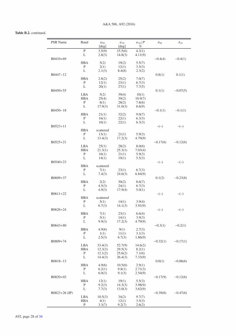
A&A 586, A92 (2016)

Table B.2. continued.

PSR Name Band w50 w10 w10/P δ50 δ10

[deg] [deg] %P 3.5(9) 15.5(6) 4.3(1)L 2.8(3) 14.8(3) 4.11(9)

B0410+69 −0.4(4) −0.4(1)HBA 5(2) 19(2) 5.5(7)

P 2(1) 12(1) 3.5(3)L 2.1(3) 8.4(8) 2.3(2)

B0447−12 0.8(1) 0.1(1)HBA 2.8(2) 25(2) 7.0(7)

P 12(1) 23(1) 6.7(3)L 20(1) 27(1) 7.7(5)

B0450+55 0.1(1) −0.07(5)LBA 5(2) 39(4) 10(1)HBA 25(4) 39(2) 10.9(7)

P 8(1) 28(2) 7.8(6)L 17.9(3) 31.0(3) 8.6(9)

B0450−18 −0.1(1) −0.1(1)HBA 21(1) 32(2) 9.0(7)

P 16(1) 22(1) 6.3(3)L 16(1) 22(1) 6.3(3)

B0523+11 –(–) –(–)HBA scattered

P 13(1) 21(1) 5.9(3)L 13.4(3) 17.2(3) 4.79(9)

B0525+21 −0.17(6) −0.12(6)LBA 25(1) 28(2) 8.0(6)HBA 21.3(1) 25.3(1) 7.03(4)

P 16(1) 21(1) 5.9(3)L 14(1) 19(1) 5.5(3)

B0540+23 –(–) –(–)HBA scattered

P 7(1) 23(1) 6.7(3)L 7.4(3) 24.6(3) 6.84(9)

B0609+37 0.1(2) −0.23(8)HBA 2(2) 30(2) 8.6(7)

P 4.5(3) 24(1) 6.7(3)L 4.9(3) 17.9(4) 5.0(1)

B0611+22 –(–) –(–)HBA scattered

P 5(1) 14(1) 3.9(4)L 6.7(3) 14.1(3) 3.91(9)

B0626+24 –(–) –(–)HBA 7(1) 23(1) 6.6(4)

P 5(1) 14(1) 3.9(3)L 9.9(3) 17.2(3) 4.79(9)

B0643+80 −0.3(1) −0.2(1)HBA 4.9(6) 9(1) 2.7(3)

P 1(1) 11(1) 3.1(3)L 2.5(3) 6.7(3) 1.86(9)

B0809+74 −0.32(1) −0.17(1)LBA 33.4(3) 52.7(9) 14.6(2)HBA 12.3(3) 29.5(3) 8.2(1)

P 12.1(2) 25.6(2) 7.1(6)L 14.4(3) 26.4(3) 7.33(9)

B0818−13 0.0(1) −0.06(6)HBA 4.9(6) 10.5(6) 2.9(1)

P 6.2(1) 9.8(1) 2.71(3)L 6.0(3) 9.1(3) 2.54(9)

B0820+02 −0.17(9) −0.12(6)HBA 12(1) 19(1) 5.5(3)

P 9.2(3) 14.3(3) 3.98(9)L 7.7(3) 13.0(3) 3.62(9)

B0823+26 (IP) −0.39(8) −0.47(6)LBA 10.5(3) 34(2) 9.7(7)HBA 4(1) 12(1) 3.5(3)

P 3.3(7) 9.2(7) 2.6(2)

A92, page 28 of 34

M. Pilia et al.: LOFAR 100 pulsar profiles

Table B.2. continued.

PSR Name Band w50 w10 w10/P δ50 δ10

[deg] [deg] %L 2.8(3) 6.0(3) 1.66(9)

B0834+06 −0.05(4) −0.16(2)LBA 7.7(3) 15.5(3) 4.3(9)HBA 6.0(3) 13.7(3) 3.81(9)

P 6.4(1) 8.8(1) 2.44(3)L 6.7(3) 8.7(3) 2.41(9)

B0906−17 0.0(3) −0.06(8)HBA 2(2) 25(2) 7.0(7)

P 6(1) 19(1) 5.5(3)L 6.7(3) 20.1(4) 5.6(1)

B0917+63 −0.18(7) −0.21(5)LBA 14(2) 20(2) 5.7(7)HBA 9.8(6) 14.1(6) 3.9(1)

P 7(2) 11(1) 3.3(4)L 6.7(3) 8.8(3) 2.44(9)

B0919+06 −0.0(1) −0.31(3)HBA 4.6(3) 22.9(3) 6.35(9)

P 8.2(6) 19.2(6) 5.3(1)L 4.2(3) 10.9(3) 3.03(9)

B0943+10 0.3(1) −0.18(3)LBA 6.3(6) 26.0(8) 7.2(2)HBA 7.0(6) 20.4(6) 5.7(1)

P 13(1) 23(3) 6.6(8)L 7(2) 13.4(4) 3.7(1)

B0950+08 (IP) −0.31(2) −0.22(2)LBA 33.0(3) 65(1) 18.1(4)HBA 16(5) 50(5) 14(1)

P 12.3(7) 28.5(7) 7.9(2)L 11.6(3) 29.2(4) 8.1(1)

B1112+50 0.1(1) −0.08(6)LBA 4.2(9) 12(1) 3.5(4)HBA 4.2(6) 9.8(6) 2.7(1)

P 2.9(6) 7.1(6) 2.0(1)L 5.3(3) 8.4(3) 2.35(9)

B1133+16 −0.16(3) −0.17(2)LBA 14.1(3) 18.3(3) 5.08(9)HBA 10.9(3) 14.1(3) 3.91(9)

P 9.8(1) 12.7(1) 3.52(3)L 1.4(3) 8.8(3) 2.44(9)

B1237+25 0.2(1) −0.15(2)LBA 1.4(6) 22.5(6) 6.3(1)HBA 1.8(3) 17.6(3) 4.88(9)

P 12.4(7) 14.6(7) 4.1(1)L 10.9(3) 13.0(3) 3.62(9)

J1238+21 0.4(4) 0.0(1)HBA 1.4(6) 9.8(6) 2.7(1)

L 3.2(4) 10(1) 2.8(3)J1313+0931 –(–) –(–)

HBA 4(1) 8(1) 2.3(3)B1322+83 −0.0(1) −0.07(9)

HBA 11(1) 22(1) 6.3(3)P 8(1) 22(1) 6.4(5)L 10.2(5) 19(1) 5.3(3)

B1508+55 0.37(8) 0.07(4)LBA scatteredHBA 4.2(3) 9.5(3) 2.64(9)

P 4.6(1) 12.6(1) 3.49(2)L 8.1(3) 12.3(3) 3.42(9)

B1530+27 −0.42(9) −0.23(5)HBA 12.0(6) 20.4(8) 5.7(2)

P 8(1) 15.1(7) 4.2(2)L 4.6(3) 12.0(3) 3.3(1)

B1540−06 −0.2(1) −0.06(7)LBA 7(1) 18(3) 5.1(8)HBA 2(1) 11(1) 3.1(3)

A92, page 29 of 34

A&A 586, A92 (2016)

Table B.2. continued.

PSR Name Band w50 w10 w10/P δ50 δ10

[deg] [deg] %P 3.3(2) 8.3(2) 2.31(5)L 2.8(3) 8.8(3) 2.44(9)

B1541+09 0.52(2) 0.44(4)LBA scatteredHBA 18.6(3) 36.6(5) 10.2(1)

P 17(3) 71(3) 19(1)L 61(1) 97(3) 26(1)

B1604−00 −0.1(6) −0.04(4)LBA 8(2) 11(2) 3.1(6)HBA 9.5(3) 14.1(3) 3.91(9)

P 10.5(6) 15.4(6) 4.3(1)L 7.4(3) 12.7(3) 3.52(9)

B1612+07 −0.0(4) −0.0(1)HBA 1.4(6) 7.0(6) 2.0(1)

P 2.3(7) 7.7(8) 2.1(2)L 1.8(3) 6.7(4) 1.9(1)

J1627+1419 –(–) –(–)HBA 23(1) 32(5) 8(1)

B1633+24 −0.1(1) −0.5(7)LBA 14(2) 18(2) 5.1(7)HBA 8(2) 28(2) 7.8(7)

P 9(1) 33(2) 9.4(7)L 9(1) 20.1(4) 5.6(1)

B1642−03 0.1(1) 0.17(5)HBA 2.8(3) 7.7(3) 2.15(9)

P 3.0(1) 6.3(1) 1.74(5)L 3.5(3) 10.2(3) 2.83(9)

J1645+1012 −0.2(2) −0.1(1)HBA 9(1) 18(1) 5.1(3)

L 6(1) 16(2) 4.5(6)J1652+2651 −0.17(8) −0.16(7)

HBA 16(1) 21(1) 5.9(3)P 14(1) 16(1) 4.7(2)L 11.6(3) 14.4(4) 4.0(1)

B1737+13 0.2(2) −0.02(7)HBA 5(1) 19(1) 5.5(3)

P 13.8(5) 22(1) 6.3(3)L 13(1) 19.7(7) 5.5(2)

B1749−28 −0.3(1) −0.25(5)HBA 6.0(3) 12.0(3) 3.32(9)

P 4.2(1) 8.0(1) 2.22(3)L 3.5(3) 7.4(3) 2.05(9)

B1818−04 –(–) –(–)HBA scattered

P 5.9(7) 16.3(7) 4.5(1)L 6.0(3) 11.3(3) 3.13(9)

B1821+05 0.95(9) 0.49(4)HBA 3.5(3) 8.8(3) 2.44(9)

P 3.2(3) 19.3(8) 5.4(2)L 22.5(3) 28.9(5) 8.0(1)

B1822−09 (IP) −0.2(1) 0.4(1)LBA 8(1) 33(2) 9.4(6)HBA 4(1) 9(1) 2.7(3)

P 4(1) 9(1) 2.6(5)L 4.2(3) 21.5(3) 5.96(9)

B1831−04 –(–) –(–)HBA scattered

P 50(7) 122(15) 34(4)L 108(2) 132.0(9) 36.7(2)

B1839+09 0.3(2) −0.0(1)HBA 8(2) 19(2) 5.5(7)

P 3.9(7) 13.2(8) 3.7(2)L 8.8(3) 14.8(9) 4.1(2)

B1839+56 0.4(1) 0.21(6)LBA 2.1(6) 5.6(6) 1.6(1)

A92, page 30 of 34

M. Pilia et al.: LOFAR 100 pulsar profiles

Table B.2. continued.

PSR Name Band w50 w10 w10/P δ50 δ10

[deg] [deg] %HBA 1.8(3) 3.5(3) 0.98(9)

P 4.3(8) 11.4(6) 3.2(1)L 6.3(3) 9.9(3) 2.74(9)

B1842+14 0.19(6) 0.12(4)LBA scatteredHBA 33.8(3) 61.9(3) 17.19(9)

P 6.7(5) 12.0(5) 3.3(1)L 7.7(3) 12.4(3) 3.44(9)

B1848+12 −0.2(2) −0.3(1)HBA 4.2(6) 11(1) 3.3(3)

P 2.4(4) 5.4(4) 1.5(1)L 2.8(3) 6.0(5) 1.7(1)

B1848+13 −0.2(2) −0.2(1)HBA 8(2) 19(2) 5.5(7)

P 5(1) 14(2) 4.1(6)L 4.9(3) 12.0(4) 3.3(1)

B1857−26 –(–) –(–)HBA scattered

P 19.3(9) 39.6(9) 11.0(2)L 30.3(3) 37.0(4) 10.3(1)

B1905+39 −0.11(4) −0.14(6)HBA 19.7(6) 26.0(9) 7.2(2)

P 16.5(7) 20.1(7) 5.6(1)L 15.1(3) 19(1) 5.5(3)

B1907+00 –(–) –(–)HBA scattered

P 1.7(4) 3.9(4) 1.1(1)L 1.8(3) 8.8(7) 2.4(1)

B1907+02 –(–) –(–)HBA scattered

P 2.7(8) 9.9(8) 2.7(2)L 2.1(3) 12(1) 3.4(2)

B1907+10 –(–) –(–)HBA scattered

P 5.7(5) 15.6(5) 4.3(1)L 6.0(3) 16.9(3) 4.69(9)

B1911−04 –(–) –(–)HBA scattered

P 2.95(9) 5.71(9) 1.59(2)L 3.2(3) 7.0(3) 1.95(9)

B1914+09 –(–) –(–)HBA scattered

P 4(1) 13(1) 3.6(5)L 12.0(3) 16.9(9) 4.7(2)

B1915+13 –(–) –(–)HBA scattered

P 4(1) 14(1) 4.1(3)L 7.4(3) 15.5(3) 4.3(9)

B1917+00 –(–) –(–)HBA scattered

P 1.4(6) 9.1(6) 2.5(1)L 1.4(3) 10.2(3) 2.83(9)

B1918+26 −0.1(2) −0.2(1)HBA 1(1) 9(1) 2.7(3)

P 7.5(7) 11(2) 3.1(5)L 6.0(6) 7.4(3) 2.1(1)

B1919+21 0.11(5) −0.02(3)LBA 5.3(3) 11.3(3) 3.13(9)HBA 7.0(3) 10.2(3) 2.83(9)

P 7.0(6) 9.8(6) 2.7(1)L 8.4(3) 10.6(3) 2.93(9)

B1920+21 –(–) –(–)HBA scattered

P 2.7(6) 13.0(6) 3.6(1)L 5.3(3) 17.2(5) 4.8(1)

A92, page 31 of 34

A&A 586, A92 (2016)

Table B.2. continued.

PSR Name Band w50 w10 w10/P δ50 δ10

[deg] [deg] %B1923+04 −0.3(1) −0.15(9)

HBA 9.1(9) 13(1) 3.7(3)P 4.9(7) 10.7(7) 3.0(2)L 4.2(3) 9.1(3) 2.54(9)

B1929+10 (IP) 0.13(8) −0.18(3)LBA 11(5) 50(7) 14(2)HBA 6.3(4) 28.1(9) 7.8(2)

P 9(1) 21.8(3) 6.06(9)L 8.8(3) 17.9(3) 4.99(9)

B1953+50 −0.2(1) −0.13(5)LBA 16(4) 14(3) 3(1)HBA 3.2(3) 10.9(3) 3.03(9)

P 2(1) 6(1) 1.9(3)L 3.2(3) 8.1(3) 2.25(9)

B2021+51 0.3(1) −0.22(5)HBA 5(1) 25(1) 7.0(3)

P 4.5(5) 21.2(5) 5.9(1)L 8.1(3) 15.8(3) 4.4(9)

B2022+50 (IP) −0.4(4) −0.5(1)HBA 5(2) 22(3) 6(1)

P 4(2) 14(2) 4.0(5)L 2.5(3) 8.1(3) 2.25(9)

B2043−04 −0.1(1) −0.0(1)HBA 4(1) 9(1) 2.5(4)

P 4.2(3) 7.6(3) 2.1(1)L 3.9(3) 7.7(3) 2.15(9)

B2044+15 0.1(3) −0.07(7)HBA 2.1(6) 9(1) 2.7(3)

P 2.8(9) 16.9(6) 4.7(1)L 2.8(3) 14.1(3) 3.91(9)

B2106+44 –(–) –(–)HBA scattered

P 18(3) 50(3) 14.0(9)L 21.1(3) 31.7(3) 8.8(9)

B2110+27 −0.3(2) −0.2(1)HBA 3.5(6) 6.3(6) 1.8(1)

P 3.3(3) 6.3(3) 1.74(9)L 1.8(3) 4.6(3) 1.27(9)

B2113+14 –(–) –(–)HBA scattered

P 6(1) 14(1) 3.9(5)L 7.0(3) 19(1) 5.3(3)

B2122+13 −0.2(2) −0.2(1)HBA 1(5) 22(2) 6.2(6)

P 15(2) 16(2) 4.7(6)L 11.6(3) 14(1) 4.1(3)

B2148+63 –(–) –(–)HBA scattered

P 18(1) 31(1) 8.8(3)L 11.3(3) 19.0(3) 5.28(9)

B2154+40 –(–) –(–)HBA 7.4(3) 33(1) 9.4(3)

P 8.5(7) 26.4(7) 7.3(2)L 14.8(3) 23.9(3) 6.65(9)

B2217+47 0.1(1) 0.1(5)LBA scatteredHBA 4.6(3) 9.1(3) 2.54(9)

P 4.7(2) 8.8(2) 2.44(7)L 5.3(3) 11.3(3) 3.13(9)

B2224+65 0.48(3) 0.22(4)HBA 11.6(3) 22.9(9) 6.3(2)

P 7(2) 48(2) 13.3(6)L 34.5(3) 44.0(4) 12.2(1)

B2227+61 –(–) –(–)HBA scattered

A92, page 32 of 34

M. Pilia et al.: LOFAR 100 pulsar profiles

Table B.2. continued.

PSR Name Band w50 w10 w10/P δ50 δ10[deg] [deg] %

P 20(1) 26(1) 7.4(3)L 2.8(3) 23(1) 6.6(3)

J2248−0101 –(–) –(–)HBA scattered

P 7.4(8) 13(1) 3.6(3)L 6.3(3) 13(1) 3.7(2)

J2253+1516 –(–) –(–)HBA 2.1(7) 22(2) 6.3(6)

B2255+58 –(–) –(–)HBA scattered

P 6(1) 24(1) 6.7(4)L 9.1(3) 20.4(3) 5.67(9)

B2303+30 −0.2(1) −0.2(6)LBA 5(2) 11(2) 3.3(6)HBA 5.6(3) 12.3(5) 3.4(1)

P 4.5(2) 8.1(2) 2.26(7)L 3.2(3) 7.4(3) 2.05(9)

B2306+55 0.43(7) −0.14(2)HBA 4.9(3) 30.6(4) 8.5(1)

P 20(1) 24(1) 6.8(4)L 16.9(3) 22.2(4) 6.2(1)

B2310+42 0.07(5) −0.07(3)HBA scatteredHBA 8.4(3) 18.3(3) 5.08(9)

P 8(1) 13(1) 3.9(2)L 9.9(3) 15.5(3) 4.3(9)

B2315+21 −0.1(1) −0.0(1)HBA 5.6(6) 7.7(6) 2.1(1)

P 2(1) 7(1) 2.0(3)L 4.2(3) 7.0(3) 1.96(9)

B2334+61 0.5(1) 0.0(1)HBA 8(2) 25(2) 7.0(7)

P 8.1(8) 22(2) 6.2(7)L 17.2(4) 25(1) 7.1(3)

Table B.3. Peak ratios.

PSR Name Band P1 P2 φ1 φ2 P2/P1B0059+65 HBA 0.28 0.96 0.47 0.52 3.41

P 0.96 0.64 0.48 0.52 0.66L 0.99 0.75 0.48 0.52 0.77

B0301+19 HBA 1.00 0.67 0.48 0.52 0.68P 0.89 1.00 0.48 0.52 1.12L 0.66 0.98 0.49 0.51 1.49

B0320+39 LBA 0.57 0.68 0.48 0.50 1.19HBA 0.54 0.79 0.49 0.50 1.46

L 0.95 0.32 0.50 0.51 0.33B0329+54 HBA 1.00 0.12 0.50 0.53 0.12

P 1.00 0.16 0.50 0.53 0.17L 0.99 0.30 0.50 0.52 0.30

B0525+21 LBA 0.87 0.70 0.52 0.58 0.80HBA 0.99 0.75 0.52 0.58 0.76

P 0.98 0.92 0.53 0.57 0.93L 0.73 1.01 0.53 0.57 1.39

B0834+06 LBA 0.97 0.70 0.50 0.51 0.72HBA 1.01 0.62 0.50 0.51 0.62

P 1.00 0.60 0.50 0.51 0.60L 0.93 0.65 0.49 0.51 0.70

B0917+63 LBA 0.62 0.85 0.48 0.52 1.37HBA 0.83 0.95 0.49 0.51 1.15

P 0.58 1.00 0.49 0.51 1.72L 1.01 0.93 0.49 0.50 0.92

B1133+16 LBA 0.71 0.97 0.49 0.52 1.35HBA 0.98 0.81 0.49 0.52 0.82

Notes. For pulsars with double and multiple peaks (Col. 1), for each frequency band (Col. 2) the amplitudes of the two most prominent peaksnormalised to the amplitude of the main peak of the profile are indicated (Cols. 3 and 4), ordered by spin phase φ (Cols. 5 and 6), and their ratioP2/P1 (Col. 7). The horizontal line in the table marks the change between previously studied cases and new (as in Fig. 6).

A92, page 33 of 34

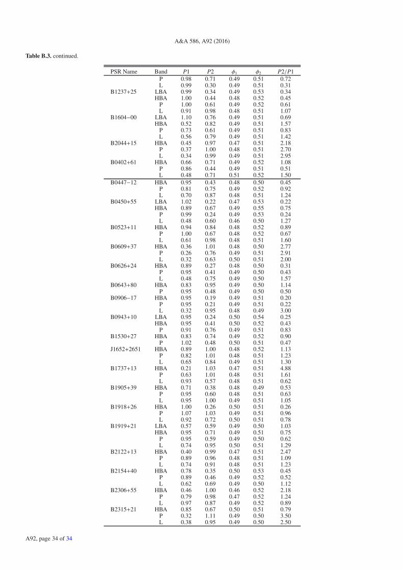
A&A 586, A92 (2016)

Table B.3. continued.

PSR Name Band P1 P2 φ1 φ2 P2/P1P 0.98 0.71 0.49 0.51 0.72L 0.99 0.30 0.49 0.51 0.31

B1237+25 LBA 0.99 0.34 0.49 0.53 0.34HBA 1.00 0.44 0.48 0.52 0.45

P 1.00 0.61 0.49 0.52 0.61L 0.91 0.98 0.48 0.51 1.07

B1604−00 LBA 1.10 0.76 0.49 0.51 0.69HBA 0.52 0.82 0.49 0.51 1.57

P 0.73 0.61 0.49 0.51 0.83L 0.56 0.79 0.49 0.51 1.42

B2044+15 HBA 0.45 0.97 0.47 0.51 2.18P 0.37 1.00 0.48 0.51 2.70L 0.34 0.99 0.49 0.51 2.95

B0402+61 HBA 0.66 0.71 0.49 0.52 1.08P 0.86 0.44 0.49 0.51 0.51L 0.48 0.71 0.51 0.52 1.50

B0447−12 HBA 0.95 0.43 0.48 0.50 0.45P 0.81 0.75 0.49 0.52 0.92L 0.70 0.87 0.48 0.51 1.24

B0450+55 LBA 1.02 0.22 0.47 0.53 0.22HBA 0.89 0.67 0.49 0.55 0.75

P 0.99 0.24 0.49 0.53 0.24L 0.48 0.60 0.46 0.50 1.27

B0523+11 HBA 0.94 0.84 0.48 0.52 0.89P 1.00 0.67 0.48 0.52 0.67L 0.61 0.98 0.48 0.51 1.60

B0609+37 HBA 0.36 1.01 0.48 0.50 2.77P 0.26 0.76 0.49 0.51 2.91L 0.32 0.63 0.50 0.51 2.00

B0626+24 HBA 0.89 0.27 0.48 0.50 0.31P 0.95 0.41 0.49 0.50 0.43L 0.48 0.75 0.49 0.50 1.57

B0643+80 HBA 0.83 0.95 0.49 0.50 1.14P 0.95 0.48 0.49 0.50 0.50

B0906−17 HBA 0.95 0.19 0.49 0.51 0.20P 0.95 0.21 0.49 0.51 0.22L 0.32 0.95 0.48 0.49 3.00

B0943+10 LBA 0.95 0.24 0.50 0.54 0.25HBA 0.95 0.41 0.50 0.52 0.43

P 0.91 0.76 0.49 0.51 0.83B1530+27 HBA 0.83 0.74 0.49 0.52 0.90

P 1.02 0.48 0.50 0.51 0.47J1652+2651 HBA 0.89 1.00 0.48 0.52 1.13

P 0.82 1.01 0.48 0.51 1.23L 0.65 0.84 0.49 0.51 1.30

B1737+13 HBA 0.21 1.03 0.47 0.51 4.88P 0.63 1.01 0.48 0.51 1.61L 0.93 0.57 0.48 0.51 0.62

B1905+39 HBA 0.71 0.38 0.48 0.49 0.53P 0.95 0.60 0.48 0.51 0.63L 0.95 1.00 0.49 0.51 1.05

B1918+26 HBA 1.00 0.26 0.50 0.51 0.26P 1.07 1.03 0.49 0.51 0.96L 0.92 0.72 0.50 0.51 0.78

B1919+21 LBA 0.57 0.59 0.49 0.50 1.03HBA 0.95 0.71 0.49 0.51 0.75

P 0.95 0.59 0.49 0.50 0.62L 0.74 0.95 0.50 0.51 1.29

B2122+13 HBA 0.40 0.99 0.47 0.51 2.47P 0.89 0.96 0.48 0.51 1.09L 0.74 0.91 0.48 0.51 1.23

B2154+40 HBA 0.78 0.35 0.50 0.53 0.45P 0.89 0.46 0.49 0.52 0.52L 0.62 0.69 0.49 0.50 1.12

B2306+55 HBA 0.46 1.00 0.46 0.52 2.18P 0.79 0.98 0.47 0.52 1.24L 0.97 0.87 0.49 0.52 0.89

B2315+21 HBA 0.85 0.67 0.50 0.51 0.79P 0.32 1.11 0.49 0.50 3.50L 0.38 0.95 0.49 0.50 2.50

A92, page 34 of 34