Embed Size (px)
Citation preview

Wide Area Power System Islanding Detection,
Classification and State Evaluation Algorithm
Rui Sun
Dissertation submitted to the faculty of the Virginia Polytechnic Institute and State
University in partial fulfillment of the requirements for the degree of
Doctor of Philosophy
in
Electrical Engineering
Virgilio A. Centeno (Chair)
Arun G. Phadke
James S. Thorp
Jaime De La Reelopez
Sandeep Shukla
Werner E. Kohler
December 14th, 2012
Blacksburg, Virginia U.S.A
Keywords: islanding, detection & identification, state evaluation,
wide area measurements, data mining, decision trees.

Wide Area Power System Islanding Detection,
Classification and State Evaluation Algorithm
Rui Sun
Abstract
An islanded power system indicates a geographical and logical detach between a portion
of a power system and the major grid, and often accompanies with the loss of system
observability. A power system islanding contingency could be one of the most severe
consequences of wide-area system failures. It might result in enormous losses to both the power
utilities and the consumers. Even those relatively small and stable islanding events may largely
disturb the consumers’ normal operation in the island. On the other hand, the power consumption
in the U.S. has been largely increasing since 1970s with the respect to the bloom of global
economy and mass manufacturing, and the daily increased requirements from the modern
customers. Along with the extreme weather and natural disaster factors, the century old U.S.
power grid is under severely tests for potential islanding disturbances. After 1980s, the invention
of synchronized phasor measurement units (PMU) has broadened the horizon for system
monitoring, control and protection. Its real time feature and reliable measurements has made
possible many online system schemes. The recent revolution of computers and electronic devices
enables the implementation of complex methods (such as data mining methods) requiring large
databases in power system analysis. The proposed method presented in this dissertation is
primarily focused on two studies: one power system islanding contingency detection,
identification, classification and state evaluation algorithm using a decision tree algorithm and
topology approach, and its application in Dominion Virginia power system; and one optimal
PMU placement strategy using a binary integral programming algorithm with the consideration
of system islanding and redundancy issues.

iii
To my parents: Ying Sun and Jin Tan

iv
Acknowledgements
First and foremost, I would like to express my deepest appreciation to my
advisor and committee chair, Dr. Virgilio Centeno, who has continually and
convincingly kept a spirit in regard to the research and teaching. Dr. Centeno has
taught me so much throughout many aspects of my study and life. Without his
patient guidance and support I cannot finish my research and have today’s
achievement.
I would like to thank Dr. Arun Phadke and Dr. James Thorp for their great
help and guidance in my researches. From them, I learned an attitude and spirit of
research and working. My appreciation also goes to Dr. Jaime De Ree and Dr.
Sandeep Shukla. They are knowledgeable and always enthusiastic to offer help.
My gratitude also goes to the Dr. Werner Kholer, Dr. Yaman Evrenosoglu and Dr.
Broadwater, for their genuine interest and support. I would also like to
acknowledge my friends, lab-mates in the Power Lab at Virginia Tech and
personals at Dominion Virginia Power. I’m honored to work with these great
minds. Special thanks to Zhe, who is always standing beside me and giving me
courage.
Last but not the least, I want to give my highest appreciation to my parents,
Ying Sun and Jin Tan, who are always the strongest support of me and my mentors
of life. No matter how far I go, they are always with me in the bottom of my heart.

v
Table of Contents
Abstract ……………………………………………………………………………………………………ii
Acknowledgements ………………....…………………………………………………………………..iv
List of Figures …………………………………………………………………………………………...vii
List of Tables ………………………………………………………………………………………..….viii
Chapter 1: Introduction ............................................................................................................... 1
1.1 The History of Islanding Scenarios ............................................................................... 1
1.1.1 Major Power System Disturbances involving Islanding ......................................... 2
1.1.2 Power System Disturbances involving Small Islanding Events .............................. 9
1.1.3 The PMU’s role in islanding Scenarios .................................................................10
1.2 Researches on Islanding Issues .................................................................................12
1.2.1 The Studies of Controlled Islanding .....................................................................12
1.2.2 The Studies of Islanding Disturbances .................................................................13
1.2.3 The Virginia Power System ..................................................................................16
1.3 Overview of the Dissertation .......................................................................................19
Chapter 2: Methodology ............................................................................................................21
2.1 The Decision Tree Algorithm in Islanding Analysis ......................................................21
2.1.1 Overview of Decision Trees .................................................................................22
2.1.2 Decision Tree Algorithm and Non-controlled Islanding .........................................33
2.1.3 Islanding Contingencies Database Creation ........................................................36
2.2 The Islanding Severity Index (ISI) ...............................................................................48
2.2.1 The Concept ........................................................................................................48
2.2.2 Adapted Real Time ISI Computation ....................................................................52
2.3 The Optimal PMU Placements using BIPA .................................................................55
2.3.1 The Introduction of PMU Placement Methods ......................................................56
2.3.2 Some Definition and Backgrounds in PMU Observability .....................................58
2.3.3 Theorems and Assumptions in PMU Placement ..................................................59
2.3.4 The Modified Bus Reduction and PMU Placement Scheme .................................63
2.3.5 Binary Integer Programming Algorithm (BIPA) .....................................................65
Chapter 3: Simulations And Results ..........................................................................................69
3.1 Testing Results on Simulated Islanding Database ......................................................69
3.1.1 Test on System Islanding Detecting Strategy .......................................................69
vi
3.1.2 Test on the modified enumeration method ...........................................................70
3.1.3 Tests on DT based Islanding Detection................................................................71
3.2 Testing Results on Islanding Severity Index ................................................................84
3.2.1 The Creation of the Islanding Database for ISI .....................................................85
3.2.2 ISI Computation and Analysis ..............................................................................88
3.2.3 Curve fitting comparison and analysis ..................................................................91
3.2.4 Adapted real time ISI computation and analysis ...................................................95
3.3 Results on the Optimal PMU Placement Using BIPA ..................................................98
3.3.1 Optimal PMU Placement ......................................................................................98
3.3.2 PMU Placement for Redundant Problem ........................................................... 100
3.3.3 The Stepwise PMU Placement Strategy & PMU Group Concept ....................... 101
Chapter 4: The Islanding Scheme in DVP System .................................................................. 102
4.1 Introduction of DVP System ...................................................................................... 102
4.2 Online Islanding Detection Module Schemes ............................................................ 107
4.2.1 Methodology ...................................................................................................... 107
4.3 Study of the Islanding Scenarios in DVP System ...................................................... 113
4.3.1 Decision Tree Analysis ...................................................................................... 114
4.3.2 Islanding Variable Importance Analytics ............................................................. 118
4.4 Islanding Analysis with the Consideration of internal PMUs ...................................... 121
4.4.1 DT Improvement Test: Region-1 ........................................................................ 121
4.4.2 DT Improvement Test: Region-2 ........................................................................ 125
4.4.3 DT Improvement Test: Region-3 ........................................................................ 126
4.5 Islanding Analysis with the Light Load Model ............................................................ 129
4.6 Analysis of Fisher’s method applied to Islanding DT Attributes ................................. 134
Chapter 5: Conclusion & Discussion ....................................................................................... 138
5.1 Conclusion ................................................................................................................ 138
5.2 Discussion & Future Research .................................................................................. 144
References ............................................................................................................................. 147
Appendix ................................................................................................................................. 150
Appendix A: Major Power System Disturbances involving Islanding .................................... 150
Appendix B: Study System Model Introduction .................................................................... 155
Appendix C: Matlab Codes for Some of the Algorithms ....................................................... 163

vii
List of Figures
Figure 1.1: Affected areas in the Gulf Coast Area Power System Disturbance ............................................................. 3
Figure 1.2: Affected areas in the BC Hydro – Vancouver Island Outage ....................................................................... 4
Figure 1.3: Affected areas in the Northridge Earthquake Disturbance ........................................................................ 5
Figure 1.4: Affected areas in the Hurricane Gustav Disturbance ................................................................................. 7
Figure 1.5: The Dominion Virginia Power Region ........................................................................................................ 17
Figure 2.1: Classification Tree Example ....................................................................................................................... 23
Figure 2.2: DT based Islanding contingency scheme ................................................................................................... 35
Figure 2.3: 8-bus 3-machine test system ..................................................................................................................... 38
Figure 2.4: 8-bus 3-machine test system with branch disconnections ........................................................................ 42
Figure 2.5: Various branch tripping locations .............................................................................................................. 46
Figure 2.6: The Islanding Analysis Method .................................................................................................................. 55
Figure 2.7: The PMU Observability Increase ................................................................................................................ 60
Figure 2.8: Virtual bus reduction ................................................................................................................................. 63
Figure 2.9: Traditional PMU placement loses observability in islanding case ............................................................. 64
Figure 3.1: Islanding detecting Strategy Logics............................................................................................................ 69
Figure 3.2: Decision tree splitting diagram using 10-fold cross validation .................................................................. 78
Figure 3.3: Machine angles oscillation of category 1 cases ......................................................................................... 80
Figure 3.4: Machine angles oscillation of category 2 cases ......................................................................................... 81
Figure 3.5: Machine angles oscillation of category 3 cases ......................................................................................... 82
Figure 3.6: Geographic diagram around the selected area ......................................................................................... 86
Figure 3.7: Islanding cut-offs around the selected area .............................................................................................. 87
Figure 3.8: Selected fitting curve samples ................................................................................................................... 92
Figure 3.9: Selected fitting curve samples (cont.) ....................................................................................................... 93
Figure 3.10: Optimal PMU sets w/wo considering islanding on IEEE-30 ..................................................................... 99
Figure 4.1: The Dominion Virginia Power Region ...................................................................................................... 103
Figure 4.2: The PJM Region Zones [51] ...................................................................................................................... 104
Figure 4.3: Structure of the Dominion Online System Monitoring and Protection Software ................................... 107
Figure 4.4: The DT Based Islanding Scheme Procedures ........................................................................................... 109
Figure 4.5: Flowchart of the Islanding Module Functions ......................................................................................... 111
Figure 4.6: Decision Tree Size Comparison (after Prune) .......................................................................................... 115
Figure 4.7: Decision Tree Size Comparison (before Prune) ....................................................................................... 116
Figure 4.8: Decision Tree Attribute Type Comparison (Tree only) ............................................................................ 116
Figure 4.9: Decision Tree Attribute Type Comparison (for all) .................................................................................. 117
Figure 4.10: Internal PMU monitors in Region-1 ....................................................................................................... 122
Figure 4.11: DT relative cost comparison in Region-1 ............................................................................................... 123
Figure 4.12: DT relative cost comparison in Region-2 ............................................................................................... 125
Figure 4.13: DT stability estimate comparison in Region-3 ....................................................................................... 127
Figure 4.14: Annual Peak Load Demand for DVP ...................................................................................................... 129
Figure A.1: IEEE 39-Bus System ................................................................................................................................. 155
Figure A.2: IEEE 30-Bus System ................................................................................................................................. 159
Figure A.3: IEEE 57-Bus System ................................................................................................................................. 161
Figure A.4: IEEE 300-Bus System ............................................................................................................................... 162

viii
List of Tables
TABLE 1.1: MAJOR ISLANDING DISTURBANCES IN NERC [1-19] ....................................................................... 8
TABLE 2.1: DATA FORMAT FOR A DECISION TREE ...................................................................................... 24
TABLE 2.2: PMU OBSERVABILITY INCREASE METHODS .............................................................................. 61
TABLE 3.1: COVERAGE TEST FOR DEPTH FIRST METHOD [29] ................................................................... 70
TABLE 3.2: STUDY SYSTEM TIELINE COMPARISON ..................................................................................... 73
TABLE 3.3: STUDY SYSTEM BUS COMPARISON ........................................................................................... 73
TABLE 3.4: SELECTED SIMULATED ISLANDING CASES ................................................................................. 75
TABLE 3.5: DECISION TREE PREDICTION SUCCESS ...................................................................................... 78
TABLE 3.6: ISLANDING SEVERITY INDEX ANALYSIS ..................................................................................... 85
TABLE 3.7: UNDERFREQUENCY SHEDDING SCHEME .................................................................................. 87
TABLE 3.8: ISI FOR THE STUDY SYSTEM ...................................................................................................... 89
TABLE 3.9: ISI WITH CURVE FITTING PARAMETERS .................................................................................... 94
TABLE 3.10: REAL TIME ISI COMPUTATION ................................................................................................ 96
TABLE 3.11: BUS REDUCTION USING MODIFIED SCHEME .......................................................................... 98
TABLE 3.12: OPTIMAL PMU SETS COMPARISON ........................................................................................ 98
TABLE 3.13: REDUNDANCY PMU SETS COMPARISON .............................................................................. 100
TABLE 4.1: MAJOR SUBSTAIONS IN DOMINION ....................................................................................... 104
TABLE 4.2: DT SPECIFICS ........................................................................................................................... 113
TABLE 4.3: DT PREDICTION SUCCESS ........................................................................................................ 113
TABLE 4.4: SUBSTATION APPEARANCE IN DT FORMATION ...................................................................... 118
TABLE 4.5: SUBSTATION IMPORTANCE IN DT FORMATION ..................................................................... 119
TABLE 4.6: INTERNAL PMUS IN REGION-1 ................................................................................................ 121
TABLE 4.7: VARIABLE IMPORTANCE COMPARISON – REGION-1 .............................................................. 123
TABLE 4.8: REGION-1 ISLANDING AREA RANK (A) .................................................................................... 124
TABLE 4.9: REGION-1 ISLANDING LEVEL DETECTION (B) .......................................................................... 124
TABLE 4.10: REGION-2 ISLANDING GEN SIZE ESTIMATE COMPARISON ................................................... 125
TABLE 4.11: VARIABLE IMPORTANCE COMPARISON – REGION-2 ............................................................ 126
TABLE 4.12: REGION-3 ISLANDING STABILITY ESTIMATE COMPARISON .................................................. 127
TABLE 4.13: REGION-1 ISLANDING STABILITY ESTIMATE COMPARISON .................................................. 131
TABLE 4.14: VARIABLE IMPORTANCE COMPARISON – REGION-1 ............................................................ 131
TABLE 4.15: NERC ISLANDING CASES OCCURANCE .................................................................................. 133
TABLE 4.16: DT PREDICTION SUCCESS COMPARISON – PREDICTION SUCCESS ........................................ 135
TABLE 4.17: DT VARIABLE IMPORTANCE COMPARISON – GENSIZE ......................................................... 135
TABLE 4.18: VARIABLE IMPORTANCE COMPARISON – STABILITY ............................................................ 136
TABLE A.1: IEEE 39-BUS SYSTEM BUS DATA AND POWER FLOW DATA ................................................... 156
TABLE A.2: IEEE 39-BUS SYSTEM MACHINE DATA .................................................................................... 157
TABLE A.3: IEEE 39-BUS SYSTEM BRANCH DATA ...................................................................................... 157
TABLE A.4: IEEE 30-BUS SYSTEM MACHINE DATA .................................................................................... 159
TABLE A.5: IEEE 30-BUS SYSTEM BRANCH DATA ...................................................................................... 160

1
Chapter 1: Introduction
1.1 The History of Islanding Scenarios
An islanded power system indicates a geographical and logical detach between a portion
of a power system and the rest of the system (which is called the main grid in some references).
A well-defined islanding scenario satisfies the following options: 1) the isolated area includes
power plants and loads; the generators are continuing to power this area after detachment, which
might possibly maintain a transient or permanent stability of the islanded region. 2) After the
isolation, the island and the main grid lose most of their observability of each other, judgments in
stability and regulation are largely performed with an absence of knowledge of the system
behavior in the other area.
A power system islanding contingency could be one of the most severe consequences of
wide-area system failures. It might result in enormous losses to both the power utilities and the
consumers. Even those relatively small and stable islanding events may largely disturb the
consumers’ normal operation in the island. The islanding duration could be as short as seconds
when the system recovers from breaker reclosing or last for several days when the physical dame
to the network is severe. Among the recorded historical islanding contingencies, many of them
were economically and ecologically catastrophic blackouts. According to NERC (North America
Electric Reliability Corporation) annually disturbance reports [1-15], since 1992, over 15 major
islanding contingency disturbances have occurred and millions of customers have been affected.
Temporary islanding events are also part of other types of disturbances. Although these
contingencies were not severe, they apparently worsened the situation and increased the
complexity of the disturbance. The research in this dissertation is motivated by these historical

Rui Sun Chapter 1: Introduction
2
cases [1-19].
1.1.1 Major Power System Disturbances involving Islanding
In this section, some major islanding scenarios in the U.S. history are analyzed. Four
particular cases are introduced in details (More information about detailed islanding cases is
introduced in Appendix. A). Most of these historical islanding events featured an under/over
frequency oscillation and unbalanced load-generation situation. For many of them, rapid load-
shedding and/or generation tripping schemes were applied to maintain the island. During this
procedure, many loads were dropped and customers inside the island were affected. Most islands
were successfully retained and restored to the system. However some failed to regain
synchronization and finally collapsed.
Gulf Coast Area Power System Disturbance, August 7, 1973
This disturbance occurred at 7:53 A.M. on Tuesday, August 7, 1973. The islanded was
generating 3745 MW and exporting 1952 MW before the event. “The upset started at a
transmission substation which cleared all its lines, followed by tripping of all lines out of the
island due to instability” [16]. Frequency began to raise and generator units Barry #5 and Crist
#6 (Fig. 1.1), which were generating 1045 MW at the moment, were tripped off simultaneously
to set the frequency at approximately 61.2 Hz under governor control. The frequency stayed at
61.2 Hz for 2 minutes then it began to fall until it reached approximately 59 Hz. The under-
frequency load shedding scheme in the islanded region operated and dropped approximately 15%
of its connected load. “Approximately 7 minutes, 25 seconds after the island formation,
transmission lines across the island boundary were reclosed by operator action via supervisory
controls. The island came into synchronism and other transmission lines across the island

Rui Sun Chapter 1: Introduction
3
boundaries were reclosed manually and by synchro-check relay action, ending the disturbance.”
[16]
Figure 1.1: Affected areas in the Gulf Coast Area Power System Disturbance [16]
BC Hydro – Vancouver Island Outage, June 4, 1993
This disturbance started at 19:01 P.M. PST on Friday, June 4, 1993 [2]. Figure 1.2 shows
the system configuration before the event. Before the event, The Vancouver Island was served by
two Malaspina-Dunsmuir 500 kV AC lines, two Arnott-Vancouver Island Terminal 230 kV DC
lines, and two Arnott-Vancouver Island Terminal 138 kV AC lines (one line was not in service at
that time). The two 500 kV lines tripped at 19:01 within 7 cycles. A lightning storm was reported
in the area at the same time and might be the cause of the tripping. The auto-reclosing of both
lines were blocked and left both lines open at Malaspina end because of a parallel current
supervision scheme which was used to prevent an out-of-synchronization reconnection situation
for the 500 kV lines. The generation on the island could meet only 25% of the island’s peak

Rui Sun Chapter 1: Introduction
4
demand and a sudden 350MW power transfer tripped the working 138 kV AC line, which was
reestablished after 27 minutes. The generation-load shortage resulted in a frequency drop to 58.4
Hz. About 730 MW of demand was lost and 37,000 customers were affected.
Figure 1.2: Affected areas in the BC Hydro – Vancouver Island Outage [2]
Northridge Earthquake Disturbance, January 17, 1994
This catastrophic disturbance was caused by a magnitude 6.8 earthquake in the early
morning on January 17, 1994 [3]. The epicenter of the earthquake was in Northridge, California.
This extensive disturbance separated the Western interconnection into five electrical regions (Fig.
1.3). Three smaller regions – the Los Angeles metropolitan area including Ventura and Santa
Barbara counties in California, central Nevada and western Utah, and the southeastern Idaho and
western Wyoming were physically isolated from the main grid and finally blacked out. The rest
of the system separated into two regions, the north-western part – central & northern California,
northern Nevada, Oregon, Washington, Montana, British Columbia and Alberta experienced low
frequency (59.1 Hz) and applied load shedding. The fifth region – Southern California, Arizona,
southern Nevada, New Mexico, Colorado, Utah and Wyoming experienced high frequency (60.8

Rui Sun Chapter 1: Introduction
5
Hz). The causes of the islands varied however all islands formed within 4 minutes after the
earthquake struck. The earthquake caused intense ground movements that damaged transmission
towers and substations, followed by multiple transmission line relay operations and transformer
sudden-pressure operations, creating the first island in Southern California. The following series
of cascading relay operations at 500 kV and 230 kV transmission networks opened the WSCC
loop, separated the system into five pieces. Three islands finally collapsed due to huge
generation-load gaps and instability conditions of the islands.
Figure 1.3: Affected areas in the Northridge Earthquake Disturbance [3]
For the whole disturbance, a total of 2.5 million customers were affected and 7,500 MW
load was lost due to the separation and following load shedding. Nearly 6,400 MW of generation
tripped. Power at most areas was restored within hours. However the restoration lasted for three
days for areas suffering physical damage and permanent repairs to some facilities in the southern
California took more than a year to be completed.

Rui Sun Chapter 1: Introduction
6
Hurricane Gustav Disturbance, September 1, 2008
This catastrophic disturbance was caused by Hurricane Gustav which made its landfall at
9:30am on January 17, 1994 close to New Orleans, Louisiana. Over 964,000 customers were
affected [18, 19]. As the storm moved inland 14 transmission lines serving the Baton Rouge and
metropolitan New Orleans areas tripped with a time span of several hours. This resulted in an
island consisting of the metropolitan New Orleans area and a corridor along the Mississippi
River between New Orleans and Baton Rouge physically disconnected from the external grid,
Fig 1.4. The island contained a load of approximately 3,000 MW and the generation capacity
was made up by plants Michoud, Ninemile, Waterford and Gypsy.
Unlike previous islanding disturbances, the formation of this island was monitored by
PMUs installed inside and outside the islanded regions. The diverging frequency was recorded
and the PMUs assisted the operators in detecting the island. Maintaining the island was
successfully accomplished by adjusting governor controls and by closely monitoring the
frequencies in the area using PMU measurements. The island stood for 33 hours before Entergy
restored the island from both the east and the west side of the island through two pairs of 230 kV
lines with the help of PMU measurements in the re-synchronization procedure.

Rui Sun Chapter 1: Introduction
7
Figure 1.4: Affected areas in the Hurricane Gustav Disturbance [18]
The previous paragraphs described four historical islanding disturbances in the U.S.
power system. The causes to the four cases were different and the size and duration of each
island also varied. However, all cases shared one common characteristic: they all experienced
one or multiple stages of under/over frequency oscillations that resulted in the inevitable
shedding of loads and/or generation. Table 1 lists most of the major islanding disturbances
recorded by NERC and other sources from 1992 to 2009.

Rui Sun Chapter 1: Introduction
8
TABLE 1.1: MAJOR ISLANDING DISTURBANCES IN NERC [1-19] Case
#
Case Date Time Region Cause GEN involved Loads
involved
Customers
affected
Restoration
1 1973.8.7 07:53
EST
Gulf Coast Area,
SCS
Cascading hidden
failure (?)
3,745MW
(1,045MW
tripped)
1,793MW
(15% shed)
7min 25sec
2 1992.1.6 15:04
PST
D.C., PEPCO Equipment failure,
S.C.
335MW
dropped
18,000 Within 3
hours
3 1993.6.4 19:01
PST
Vancouver Island,
BC Hydro
Weather: Lightning 730MW lost 37,000 27min
4 1994.1.7 04:31
EST
WSCC Natural: Earthquake 5 Islands (3
collapsed)
6,400MW lost
7,500MW lost 2,500,000 3hours-3days
5 1994.
12.14
01:25
MST
WSCC LG fault caused
cascading tripping
5 Islands
11,300MW lost
9,336MW lost 1,700,000 10min-4hour
6 1996.
3.12
Peninsula Florida Weather: Cool
temperature
GEN Planned outage
12,588MW
(784MW
dropped)
9,932MW
(3,440MW
dropped)
90sec
7 1996.7.2 14:24
MST
WSCC LG fault caused
cascading tripping/
faults
5 Islands
2,000MW
dropped
Over
8,000MW
dropped
Over
1,600,000
10min-
2.5hour
8 1996.
8.10
15:48
MDT
WSCC Weather: hot
temperature
4 Islands
21,570MW
dropped
28,840MW
lost
7,446,000 90% within 5
hours
9 1997.
6.20
20:27
EDT
Potomac Electric
Power
Equipment failure 482MW 350MW 18,000 Within 2.5
hours
10 1998.
6.25
01:34
CDT
MAPP, NPCC LG fault
Weather: Lightning
3 Islands
4,270MW
removed
950MW shed 152,000 1.5hour
11 2001.
11.14
06:45
CDT
Northeastern
Wisconsin/ Upper
Michigan Peninsula
Natural:
Tree growth;
Planned line outage
742MW 1,000MW
(263MW
shed)
36min
12 2002.
4.29
15:50 Jacksonville Electric
Authority
Equipment failure
caused
Chain failure
Island collapsed
(load shedding
failed to work)
1,729MW lost Most of
365,000
60% in
36min-8hour
13 2002.
12.26
12:02
PST
WECC Weather: Ice HVDC remain
(285MW
Internal QF
tripped)
1,567MW
(950MW lost)
140,000 36min
14 2003.
3.22
6:50
PST
WECC-NWPP,
BCHA
Line fault HVDC
remained
135,000 2hour 24min
15 2005.
9.21
8:33
PDT
WECC-NWPP,
BCHA
Human Error 291MW tripped no 19min
16 2006.
7.24
15:28
PDT
WECC-NWPP,
BCTC
Weather: Lightning 525MW tripped Neighboring
system shed
650MW
26min
17 2007.
1.23
13:46
PST
WECC-NWPP,
BCTC
Human Error 2935MW lost 1000MW lost 90,000 Till 6pm
18 2007.
11.04
9:31
EDT
NPCC-HQ Weather: Tropical
Storm Noel
Island collapsed 1039MW lost 20,000 2hour– the
same day
19 2008.9.1 WECC-New Orleans Weather: Hurricane
Gustav
Over 5000MW 3000MW 964,000 33hour –
3days
The analysis to the major islanding disturbances has indicated that the causes to islanding
events are variable. If we conclude, there are several major contributors: 1) Equipment failures

Rui Sun Chapter 1: Introduction
9
caused cascading line and generator tripping actions; 2) Faults or extreme weather conditions
(Lightning, ice, and hot weather, etc) caused cascading line and generator tripping actions; 3)
Natural disasters (hurricane, earthquake, and Tropical storm, etc); and 4) Human errors, which
also include incorrect operations during the island maintaining and bad-considered
determinations on planning line/generation outages.
1.1.2 Power System Disturbances involving Small Islanding Events
According to the NERC’s annual disturbances report, small islanding conditions occurred
in quite a number of disturbance cases. The small islanding conditions indicate the islanded area
is relatively small (usually consisting of loads below 100MW) and could maintain power balance
with internal generation and loads. The small islanding events mostly happened in areas
surrounding certain plants. Such cases appearing in [12-15] normally experienced slight or no
load loss and were restored and re-synchronized with the main grid within 2 hours after the
isolation.
In the proposed research, these events are treated the in the same way as major islanding
disturbances. Because they feature all the characteristics of a massive islanding event: physically
disconnection from the main grid; consisting of both generations and loads; and experiencing
frequency oscillations and power balance adjustments. These event are of interest for this
research because: 1) these cases happen at relatively low transmission voltage levels (115kV and
below) that have lower chance for the wide area measurement system (whose devices are mainly
installed at 500/230kV transmission networks) to access the information in such area when they
isolate from the main grid; and 2) these events occur more frequently than the major islanding
disturbances.

Rui Sun Chapter 1: Introduction
10
1.1.3 The PMU’s role in islanding Scenarios
The phasor measurement unit (PMU) or synchrophasor may be one of the most important
inventions in the power systems area in the 20th
century. The PMU was invented in 1988 by Dr.
Arun G. Phadke and Dr. James S. Thorp at Virginia Tech. A PMU is a device which measures
electrical signals (voltages and currents) on an electricity grid, using a common time source for
synchronization. Time synchronization allows the power system operation center to utilize
synchronized real-time measurements of multiple remote points on the grid [20, 21] and obtain a
snapshot of the state of the system.
The PMU features such characteristics as high accuracy, fast data transmission, and wide
area system observability. Conceptually the GPS-synchronized PMU measurements could
achieve better than 1 microsecond in time accuracy and better than 0.1% in magnitude accuracy.
The reporting rates vary from 1 to 60 times per second but 30 times per second seems to be the
preferred rate by utilities. They can be used in many applications in power system generation,
transmission and distribution. These applications include real-time monitoring of the system,
real-time state measurements and the monitoring of disturbance, state estimation, system
transient stability monitoring and wide-area protection. All PMUs follow the 2005 IEEE
C37.118 standard (lately revised in 2011 as C37.118.1, 2 and published by IEEE in 2011), which
deals with issues concerning the use of PMUs in electric power systems. The standard specifies
the PMU measurements, the method of quantifying the measurements, testing & certification
requirements for verifying accuracy, and data transmission format and protocol for real-time data
communication.
In recent years, with the rapid implementation of PMUs in the major power system grids
in the U.S, the wide area monitoring system (WAMS) has become possible. The WAM System

Rui Sun Chapter 1: Introduction
11
can enhance the following functions [33] under stress or emergencies conditions: a) power
oscillations monitoring, which in the long run can help enhance power systems stabilizers (pss)
tuning and necessary operating actions as load shedding; b) voltage stability monitoring, that can
help in providing better reactive power support; and phase angle difference monitoring, that can
detect possible network separation sand help in line-reclosing or system restoration.
The PMUs have already proven their contribution in islanding events. According to the
reports from Energy Transmission, Inc and TEPCO [18-19, 28], the phase measurement system
successfully detected the possibility of island formation and informed the danger to protection
devices in several severe contingencies. In the 2008 Hurricane Gustav case, with PMUs
implemented inside/outside the island, the formation of the island was detected by Entergy
operators through reading of the diverging frequency. The PMUs successfully assisted the
operators in maintaining the island via adjusting governor controls by offering close-up and
accurate frequencies measurements. The PMU measurements also contributed in the re-
synchronization procedure.

Rui Sun Chapter 1: Introduction
12
1.2 Researches on Islanding Issues
1.2.1 The Studies of Controlled Islanding
The present researches related to the power system islanding issue are divided into two
major categories: controlled islanding and uncontrolled islanding [23]. Controlled islanding
works as a strategy in separating a severely disturbed power system into several islands, in order
to prevent an eventual collapse of the whole system. The islands are considered to be self-healing
and the formation of the controlled islands is predetermined based on grouping the generators in
the same island via their static and dynamic characteristics. Such grouping strategies include
minimum load-generation unbalances, slow-coherent generators, etc.
The term “controlled islanding” was introduced by H. You, V. Vittal and X. Wang in [57,
58], they authors analyzed the stability margin of the power system and developed automatic
islanding formation scheme based on weak connections within certain region and an analysis of
slow coherent generator groups. In [58], the authors combined the controlled islanding protection
scheme with the frequency decline-based load shedding in order to prevent the system from
collapsing under severe stress situations.
In One study, N. Senroy and V. Vittal identify and analyze the behavior of controlled
islands based on the formation of slow coherent groups of generators under an islanding
contingency [23]. They have discovered that slow coherent generators tended to separate from
the rest of the system in well defined and consistent groups. And each critical group of machines
separating from the system corresponds to a particular mode of instability. The behaviors of
different groups vary distinctly in the final stability condition. The options could be extreme
stable, disturbed stable or instable.

Rui Sun Chapter 1: Introduction
13
In another research, R. Diao and V. Vittal define islanding cases using slow coherent
generator grouping and minimum power imbalance on a study of the 16,100 bus Eastern power
grid of North America [24]. They draw the conclusion that the controlled islanding is the last line
of defense to stabilize the whole power system and provides a promising control strategy under
stressed system conditions.
Another islanding method is a three-phase method using online search for splitting
boundaries for large scale system based on Ordered Binary Decision Diagram [25, 26]. This
method considers an interconnected power system as a graph and looks for branches that will
create logical islands when tripped. The OBDD method can easily represent the balances
partition problem and perform an enumeration searching at whole space of the system.
1.2.2 The Studies of Islanding Disturbances
The islanding disturbances, on the other hand, are more complex to study. It refers to the
island(s) created against the utility’s planning. It is a power system disturbance rather than a
protection scheme. The difficulty to distinguish the islanding situation in real time is because it
influences both the stability and the structure of the system, making it obscure to monitor.
Furthermore, the potential locations and sizes of the islands remain unclear. In one study of
cascading hidden failures, H. Wang and J. S. Thorp has examined over 170,000 blackouts by
characterizing the cases as a tree-search problem and defined a random search algorithm with
certain thresholds [43].
As discussed in Section 1.1.1, there are many possible reasons to cause an islanding
contingency: a series of cascading hidden failures or multiple lines and generation tripping due to
faults, human errors, extreme weather conditions, or natural disasters like earthquakes, tropical
storms or hurricanes. It is often considered as a spontaneous phenomenon and typically starts

Rui Sun Chapter 1: Introduction
14
from the electrical centers in a power system [27] while the geographical characteristics are also
of concern. Another important issue is maintaining the island stability after its formation. The
situation becomes worse when the system’s observability is not fully achieved. Without the
certainty of the size and the location of the island, the analysis of the load-generation balance
condition and the corresponding frequency bias between the main grid and the isolated area
cannot be eliminated. Historically, the utilities and operators have made lots of efforts when
facing islanding disturbances. Logically, for an islanded power system, the primary goal is to
balance the generation and loads to decrease the chance of further loss of frequency synchronism,
preventing the island from collapsing. At the same time, maintaining the maximum firm demand
for the island to prevent customers’ losses. Possible schemes include load shedding, capacitor
and shunt switching, branch tripping and/or generation rejection. (For large natural disasters like
tornado and hurricane, some actions can be done prior to prevent the loss, including set
generators on hot standby or let them serve only the station load.) The under/over-frequency
protection schemes have been proven to be the most efficient operation for most generation
deficiency islanding situations and could effectively prevent frequency oscillation. The major
drawback is that significant generation and loads have to trip during the process and permanently
lost till the island is re-synchronized, even in those generation abundant conditions. In many
cases, the frequency jumped back and forth between the high and low limits and caused the
protection scheme trip loads and units multiple times. This is believed partially cause because the
islands were detected and identified much later after their formation thus greater effort was
required to drive the frequency back to nominal. In some cases, the operators were unaware of
the separation till the under-frequency scheme took place. In contrast, the fast detection of the
island helps the operators take correct and fast reaction to maintain the island stability. The

Rui Sun Chapter 1: Introduction
15
recent Hurricane Gustav disturbance has perfectly demonstrated that: the Entergy operators
identified island formation at the first place via PMU frequency measurements. Several units
were set as hot stand-by and some others tripped off the network for safety consideration. The
island stood for 33 hours perfectly maintained and no additional load shedding was required [18,
19].
In the research area, the detection of islanding is of most concern. TEPCO have
developed a scheme detecting power system islanding using the voltage angle differences
between PMUs [22, 28]. According to their research, the frequency scheme is not as sensitive as
the angle scheme [28]. The reaction time for judging an islanding case varies by different system
operating conditions, the scale of the system and other aspects. In the real cases tested in TEPCO
network, the phase system spent 0.27s and 0.4s to identify the islanding and a protecting action
took place immediately stopping the system from islanding. [22]
In another paper published in 1994, the author presents an island AGC function to detect
the island by computing the frequency bias using the generator parameters and the optimal 60Hz.
This function could also apply corresponding load shedding or generator tripping scheme to
maintain the island stability.
Some researchers have concentrated on the system topologies in determining the
system’s detaching status and thus identifying the islands. O. Mansour, A.A. Metwally, and F.
Goderya has introduced a full matrix algorithm [55, 56] using the Boolean algebra computed on
the system’s connectivity matrix. The full matrix obtained through booleanly multiplication is
filled with all 1s or remain constant, indicating the system’s connectivity condition. System with
islands can be distinguished by analyzing the zero conditions of the final matrix.

Rui Sun Chapter 1: Introduction
16
In [56], the authors modified the full matrix method with two successive methods. The
row-sweep method applies Boolean multiplication only to the rows of the system connectivity
matrix and studies the zero conditions of the final. A system is considered islanded when the
final vector has zero elements. The method has reduced computation time compared to the full
matrix method. The other method the authors introduced is called row-sum method which took
one step further in simplifying the row multiplication by replacing the two rows with non-zero
Boolean multiplication results with one row of Boolean summation of the two. It in some extent
fatherly reduced computation iterations and time.
One recent research on this issue is using decision tree (DT) algorithm to apply an
enumeration islanding analysis in desired islanding locations selected within the study system
[29]. The author enumerated and simulated every potential islanding contingency case to form a
database for the DT use.
1.2.3 The Virginia Power System
The islanding analysis method introduced in this dissertation is inspired by the historical
events that happened nationwide. This research is a part of the PMU measurements application
study which is sponsored by the Dominion Virginia Power (DVP) & the U.S. Department of
Energy (DOE). In this project, the online system state monitoring and protection software is
going to be installed on one DVP server and deal with real time synchrophasor measurements
from various substations located in the DVP system. The islanding module’s major task is
working out an effective online scheme for islanding detection and identification. The major area
this project will be implemented to is the Virginia mountain territory belonging to the Dominion
Virginia Power. The DVP’s transmission and distribution region is shown in Fig. 1.5.

Rui Sun Chapter 1: Introduction
17
Figure 1.5: The Dominion Virginia Power Region
The Virginia Power system is geographically dispersed with several major generation and
load centers, which can be seen via the area diagram. According to [17], some portions of the
transmission system are more heavily loaded than others. This may become the major weak point
to the system in case it splits into parts because the islanded area may face unbalance generation-
load situations. At the same time, The Virginia Power system is along the east coast of the
United States, and is easily disturb by hurricanes, windstorm and thunder storms. These severe
weather conditions are major causes in tripping of heavily loaded transmission lines. One of the
recent cases was caused by Hurricane Irene which made its landfall over Eastern North
Carolina's Outer Banks on the morning of August 27, 2011. This powerful Atlantic hurricane
caused one of the major 500kV transmission lines in DVP to trip. This line was carrying 250MW
at the moment and the tripping lasted over 1 min.
Model simulation have shown than under certain circumstances, the two aspects may
interact and result in additional cascading trips, forming island within the DVP areas.
Historically no islanding disturbance has been reported in the DVP. The closest case was a

Rui Sun Chapter 1: Introduction
18
severe disturbance that happened close to the Yorktown station that caused the plant to shut
down. However the engineering studies indicate that the possibility for islands formation within
the Virginia Power system exists.
A detailed introduction of the DVP system is given in Chapter Four.

Rui Sun Chapter 1: Introduction
19
1.3 Overview of the Dissertation
The proposed method presented in this dissertation is primarily focused on detecting and
analyzing power system islanding contingencies using online PMU measurements and related
issues including islanding stability assessment and optimal PMU placement with the
consideration of islanding.
Chapter One has introduced the history of wide-area islanding disturbances in the U.S.
power grid, and summarized previous researches related to the islanding issue. The research
works are categorized into controlled islanding protection scheme and non-controlled islanding
disturbances. A discussion about the Virginia power network is also raised.
Chapter Two discussed the principles of the proposed DT based Islanding detection,
classification and evaluation method. The primary method is composed of an intelligent decision
tree for islanding detection and identification basing on a database of system’s simulated and
practical operation and contingency records, system geographical information, and a severity
index. The DT is generated from the islanding contingency database to: distinguish an islanding
scenario from other system events as short circuits, line-tripping or generator-tripping only
basing on the state variables changes from outside the island; estimate the stability condition of
the island and locate the approximate islanded area; and help in deciding the PMU placements
for a better islanding detection and identification. The chosen methodology to grow DTs in the
proposed method is CART (Classification and Regression Trees) [37].
Another issue touched in the proposed method is the optimal PMU placement strategy
with the consideration of islanding issues and redundancies. In this chapter, some optimal PMU
placement assumptions and theorems are derived and discussed and the modification in PMU
placement strategy and power system bus reduction scheme is made. A fast and accurate method

Rui Sun Chapter 1: Introduction
20
using binary programming method to solve PMU placement problem with consideration of
islanding conditions is introduced.
Chapter Three examines the proposed decision tree algorithm in islanding detection,
estimation and classification with wide-area system model. The tests are carried out on the
precision of the system islanding detecting strategy and modified depth first method, the
efficiency and accuracy of the decision tree on islanding judgment, and the transient behaviors of
the islanding severity index. The optimal PMU placement strategy using binary integer
programming algorithm is also tested and analyzed.
Chapter Four introduces the practical utilization of the DT based islanding scheme in
the Dominion Virginia Power (DVP) system. The islanding analysis is part of the PMU
measurements application study which is sponsored by the Dominion Virginia Power & the U.S.
Department of Energy. In this project, online system state monitoring and protection software is
being installed on Dominion’s server for processing real time synchrophasor measurements from
various substations located in the DVP system. The islanding module adopts an efficient online
scheme in detecting any potential islanding failures that may happen in the DVP system. The
principle and operating procedures of this scheme are fully described and series of tests and
analytics are applied.
Chapter Five summarizes the main contributions of this research work and suggests
possible topics that can be explored in the future.

21
CHAPTER 2: METHODOLOGY
2.1 The Decision Tree Algorithm in Islanding Analysis
In this section, the utilization of the DT algorithm in islanding contingency detection and
classification and an islanding behavior analysis arefully demonstrated.
A decision tree is an inductive learning data-mining algorithm that draws the underlying
mechanisms and hidden relationships from the created database through the input-output paired
model construction process. This is achieved through a simple yet clever way: decision rules are
developed through performing a binary partitioning with the aid of series of if-else judgments.
The complete instruction of the DT theory can be found in [37] and [38]. According to a recent
overview on applications of data mining to power systems given by [39], the Decision Trees are
used as the preferred method in 86.6% of the papers.
The DT method has been used in a wide range of areas in power systems, such as security
assessment, load forecasting, state estimation, etc. The DT algorithm is already widely used in
the controlled islanding studies. In [23], the DT is trained to predict the controlled island’s
transient stability. Generated offline, the DT is considered quickly accessible to monitor the
system online performance and predict the separation. In [24], each DT is trained only for a
specified critical contingency that can potentially cause cascading events and high prediction
accuracy is obtained. For islanding scenarios, the DT is generated offline via the enumerated
islanding contingency simulation of the study system [30], and purposed for online wide area
system monitoring and detecting islanding contingencies using synchrophasor measurements.
The chosen methodology to grow DTs in the proposed method is CART (Classification
and Regression Trees). It’s mainly on classification trees due to the nature of the problem. CART

Rui Sun Chapter 2: Methodology
22
performs an exhaustive search over all data channels (attributes) and all possible splitting values
to grow the optimal tree.
2.1.1 Overview of Decision Trees
2.1.1.1 The Formation of a DT
The Decision Tree is a carrier of inductive reasoning. The algorithm has made an
investigation of the dataset, extracting the underlying mechanism given rise from the data, and
deriving a model that carries the information and past experiences, which are repeatable, to
satisfy certain pre-determined judgment requests on targets. The DT is tree-like, with multiple
nodes, branches and terminals. Fig. 2.1 depicts the schematic structure of one example
classification tree. The upmost node is called the “root” of the DT. The whole tree grows out
from this node. The node contains certain quantity of the samples in the dataset. At each node t,
the samples are split into two subsets tL and tR (the left and right child) basing on certain
judgment made upon samples’ differences at certain attribute. A splitting value for this attribute
at this node is obtained. The splitting process will iterate until no more split is possible. The
ending node is called a “terminal” node. The final classification decision is made with the
terminal nodes. In Fig. 2.1, the two colors of the terminal nodes indicate the two opposite
judgment/decisions on certain attribute. In certain cases, the DT may have multi-way splits at
one node. Multi-way splits tend to fragment the data too quickly which leads to a less efficient
split on the next level [40].

Rui Sun Chapter 2: Methodology
23
Figure 2.1: Classification Tree Example
After building the tree, when classifying a new case, the new sample is dropped off at the
root of the tree. By comparing with the splitting values at each node, the sample will eventually
fall into one terminal; one route across the tree is built and the decision is obtained.
According to [37], Decision Trees are grown through a systematic method known as
recursive binary partitioning; a "divide-and-conquer" approach where successive questions with
yes/no answers are asked in order to partition the sample space [40].
2.1.1.2 Sample Data Format
The sample data are in matrix {X} format and saved in tables. The matrix is composed of
a set of n+1measurement vectors:
TxxxX n ,,...,, 21 (2.1)
Rui Sun Chapter 2: Methodology
24
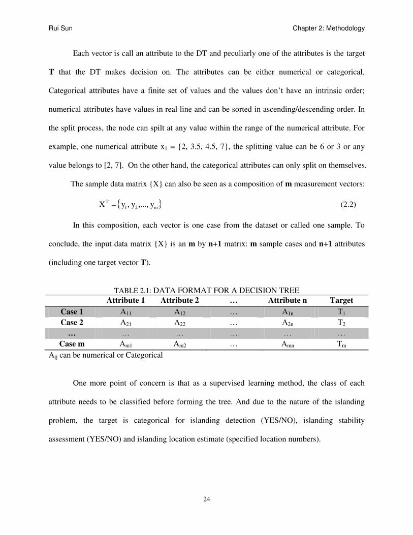
Each vector is call an attribute to the DT and peculiarly one of the attributes is the target
T that the DT makes decision on. The attributes can be either numerical or categorical.
Categorical attributes have a finite set of values and the values don’t have an intrinsic order;
numerical attributes have values in real line and can be sorted in ascending/descending order. In
the split process, the node can spilt at any value within the range of the numerical attribute. For
example, one numerical attribute x1 = {2, 3.5, 4.5, 7}, the splitting value can be 6 or 3 or any
value belongs to [2, 7]. On the other hand, the categorical attributes can only split on themselves.
The sample data matrix {X} can also be seen as a composition of m measurement vectors:
m
TyyyX ,...,, 21 (2.2)
In this composition, each vector is one case from the dataset or called one sample. To
conclude, the input data matrix {X} is an m by n+1 matrix: m sample cases and n+1 attributes
(including one target vector T).
TABLE 2.1: DATA FORMAT FOR A DECISION TREE
Attribute 1 Attribute 2 … Attribute n Target
Case 1 A11 A12 … A1n T1
Case 2 A21 A22 … A2n T2
… … … … … …
Case m Am1 Am2 … Amn Tm
Aij can be numerical or Categorical
One more point of concern is that as a supervised learning method, the class of each
attribute needs to be classified before forming the tree. And due to the nature of the islanding
problem, the target is categorical for islanding detection (YES/NO), islanding stability
assessment (YES/NO) and islanding location estimate (specified location numbers).

Rui Sun Chapter 2: Methodology
25
2.1.1.3 Tree Growing Techniques
Before the discussion of the tree growing techniques, several definitions in the DT
algorithm are introduced first. These definitions are:
1) Node Impurity
It is defined as the criterion a DT uses to rank candidate splits, or called the heterogeneity
of a node. The purity, on the other hand, is a measurement of the class homogeneity. In [41],
there is an example for the preparation to compute the node impurity: a classification tree is
grown on a categorical target variable T taking on values j = 1... J. Every node in the tree is
identified by the symbol t, and each node will have an estimated probability distribution for the
values of the target variable. There assuming J = 3, at every node we are able to specify the
probability of observing T= 1, T= 2, and T= 3 in that node and their probabilities are written p(1 |
t), p(2 |t) and p(3 | t), where the probability is conditional on the node under consideration. If the
priors are proportional to the data, then these probabilities can be taken to be the observed
relative frequencies of each class in the node. [41] The node impurity is computed based on the
probability distribution for each node.
2) Cost and Relative Cost
The DT algorithm determines the best tree by testing for error rates or the
“misclassification cost”. Considering a data sample containing 50 cases, among them the targets
have 20 categorical value As and 30 categorical value Bs. If the tree only contains one node
(actually no tree formed), all targets fall into the B-category. The misclassification cost or error
rate is 0.4 (40%). If the tree has two nodes, the terminal 1 contains 2 As and 22 Bs and seen as B-

Rui Sun Chapter 2: Methodology
26
category and terminal 2 contains 18 As and 8 Bs and seen as A-category. The new error rate is
computed as, noticing the As contains 0.4 of the total sample and Bs contains 0.6:
For Terminal 1: (2+22)/50*(2/(2+22)) = 0.04
For Terminal 2: (18+8)/50*(8/(18+8)) = 0.16
Total: 0.04+0.16 = 0.2 (20%)
The relative cost shows the improvement for a tree which is further grown from the
previous stage, a tree with single node is assigned a relative cost of 1. Using the previous
example, the error rate for the two-node tree is 0.2, so the relative cost is computed as:
0.2(new) /0.4(old) = 0.5
The relative cost shows the relationship between the misclassification costs of the mother
tree and the child tree. And it is capable in determining the best tree. The relative cost should be
smaller than 1 indicating a more efficient tree is grown after new splitting, otherwise the new
splitting is judged as inefficient. If we plot the cost and relative costs of a growing tree versus the
number of nodes, the optimal tree is the one with the smallest misclassification cost and at the
point when the first order differential of the relative cost curve reaches zero.
3) Cost Complexity
This parameter measures the tradeoff between error rates and tree sizes [40], Breiman,
Friedman, Olshen and Stone suggest the following cost complexity measure for any tree [41]:
Cost Complexity = Re-substitution Misclassification Rate +α(Num. of Terminal Nodes)
(2.3)
Where: the re-substitution relative cost measures the misclassification rate for the data
used to grow the tree (the learning pool);

Rui Sun Chapter 2: Methodology
27
α is the penalty imposed per additional terminal node.
The process of growing the correctly-sized tree consists of three stages, or three major
concerns: 1) How to determine the splitting rule basing on accurate and efficient splitting
criterion; 2) How to decide a stopping rule for the split process when terminals are reached; and
3) How to assign a class to each terminal node [40].
The first question can be solved by computing the purity /impurity of the nodes. The
ultimate goal of a DT is to extract the target vectors into the classification groups which achieve
a smallest misclassification error. In other words, achieve a maximum purity of one class of the
target vector and the minimum impurity of the equal proportion of all classes in the target vector.
When a split achieves the minimum impurity (which is mathematically equal to maximum purity,
and is easier for computation) for it descendent nodes, we can say this split is optimal for itself.
Many researchers have proposed methods for measuring mode impurity in the last two decades.
These methods include: Gini Index, Entropy Impurity, the Twoing criterion, etc. According to
[32], the choice of a particular impurity function has very little effect in the forming of the final
tree.
The two methods used in the CART® software are introduced below:
1) The Gini Impurity Criterion
The Gini impurity criterion is given by:
i(t) = 1 –S (2.4)
Where S is the sum of squared probabilities p (j | t) summed over all levels of the
dependent variable at the node t:

Rui Sun Chapter 2: Methodology
28
J
j
j tTpS1
2 )/( (2.5)
If one node consists exclusively of a single class, one of the class probabilities will equal
1, the remaining class probabilities will all equal zero, and the computed diversity index i(t) is
zero.
An optimal split s at node t is should satisfy the option to maximize the decrease in
impurity at node t achieved by split s:
)()()(),( RRLL tiptiptitsi (2.6)
While the tL and tR are left and right child node of the existed node t; pL and pR are left
and right proportions from the original node t.
2) The Twoing Criterion
CART also utilizes another splitting criterion called the Twoing criterion. This is a
measure of the difference in probability that a class appears in the left descendant rather than the
right descendant node [41]. The method is based on a concept of class separation between the
left and right child nodes. One optimal split s at node t should maximize the follow equation:
J
j
RLRL tjptjp
pptsT
1
2
)()(4
),( (2.7)
In concept, this method wants to distinguish a class j of the target between the two child
nodes that it achieves the probability that j goes to the left child node differs mostly from the
probability that j goes to the right. The rule sums the absolute value of the probability differences
over all j classes.

Rui Sun Chapter 2: Methodology
29
Once a best split is found, the DT repeats the search process for each child node,
continuing recursively until further splitting is impossible or a terminal is reached. A
methodology to declare terminal nodes is needed. The method is called the “stopping rule”. This
is a rule or set of rules that define the termination condition for the splitting. According to [41],
every stopping rule examined is shown to produce bad results, “because a node that might not
split well at one level might yield very informative splits if the tree-growing process continued
just a little further.” Nevertheless, two stopping rules are introduced below:
1) There is one effective stopping rule that terminates the splitting when the sample
number at one node is below certain threshold. It’s simple but sometimes inaccurate because
some potential child nodes with high impurity decrease are not considered under such rule.
2) Another heuristic stopping rule is to test the impurity decrease between the mother
node and the descendents. If the ),( tsi , where is impurity decrease threshold, the node is
identified as a terminal.
The CART program, on the other hand, uses a total different strategy to grow the tree.
CART has no stopping rules at all. The tree is grown to its maximum size and to be pruned to
optimal size afterwards. The CART features are introduced in the next section.
2.1.1.4 The Classification and Regression Tree (CART) Software
A major innovation of CART is to eliminate stopping rules altogether [41]. Instead of
asking when to stop, CART continues to grow the tree till further splitting is impossible, which is
called a maximal tree. After obtaining the maximal tree, CART prunes back and removes
excessive branches until it reaches the optimal tree, based on the cost complexity characteristic
of the tree.

Rui Sun Chapter 2: Methodology
30
The CART’s law to grow the maximal tree is set based on the Gini Impurity Index, as:
1) Define the minimal number of cases that is allowed for an un-terminal node (typically
5 or 10);
2) Considering the sample dataset is an m line (m cases) by n+1 column (n attributes
and one target) matrix (see Section 2.1.1.2),setting potential splitting values for
certain attribute l at node t, if the attribute vector is written as {xl,t(k)}(k = 1, 2,…, m,
},...,2,1{ nl ). When xl,t(k) is a numerical attribute, all m attribute values are sorted in
ascend. The potential split values Sl,t = {sl,t (k)} (k = 1, 2,…, m) are:
2
)1()()(
,,
,
kxkxks
tltl
tl (2.8)
When xl,t(k) is a categorical attribute, the potential split values are the attribute itself:
Sl,t = {xl,t(k)} (k = 1, 2,…, m)
3) Compute the decrease in impurity for the split at node t into two child nodes. To
achieve this, the subsets of the samples at node t into descendent left (L) and right (R)
node are defined as:
})({
})({
,,
,,
kltlR
kltlL
Sifkxt
Sifkxt
for numerical attribute (2.9)
Or
})({
})({
,,
,,
kltlR
kltlL
Sifkxt
Sifkxt
for categorical attribute (2.10)
The decrease in impurity is computed using (2.6):
)()()(),( LLLL tiptiptitsi

Rui Sun Chapter 2: Methodology
31
While the tL and tR are left and right child node of the existed node t; pL and pR are
left and right proportions from the original node t.pL and pR are computed as the total
case number at the left and right child node over the total case number at node t:
)(
)(
)(
)(
tn
tnp
tn
tnp
RR
LL
(2.11)
At any node t, the probability that one of its belonging cases belongs to the target
class Tj is computed by the re-substitution estimator:
)(
)()(),(
j
jt
jTn
TnttTp (2.12)
n(Tj) is the number of class j target, n(Tj) is the number of class j target falls into
node t, π(t) is called the prior probability of node t, if not assigned by modeler,
n
Tnt
j )()( .
And: )(
),()(
tp
tTptTp
j
j (2.13)
Where p(t) estimates the probability that a case falls into node t.
4) Step 2) and 3) iterates with the consideration of step 1) until no more split can be
performed. Then at each terminal, a series of )( tTp j (j = 1, 2… J) of all J target
classes are computed, the terminal will be assigned as class Jmax terminal with the
highest )( tTp j value: )(max)( max tTptTp jj
J .
The maximal sized DT is likely to be over-fitting for an actual problem. CART always
prunes the tree to achieve a best tree. The judgment for pruning process used in CART is the cost

Rui Sun Chapter 2: Methodology
32
complexity that introduced in Section 2.1.1.3. This parameter measures the tradeoff between
error rates and tree sizes and is defined as:
Cost Complexity = Re-substitution Misclassification Rate + α(Num. of Terminal Nodes)
Where: the re-substitution relative cost measures the misclassification rate for the data
used to grow the tree (the learning pool); and α is the penalty imposed per additional terminal
node.
Tracing back from the maximum node number to the single node, the cost complexity at
every stage of the tree are computed and the best tree is selected based on the smallest cost
complexity.
As a professional data-mining software and the most popular DT algorithm based
software, CART exhibits several advantages [41]:
1) CART uses multiple sophisticated methods to assess its accuracy.
The preferred method to assess accuracy is to use a separate test data set (usually 10% the
size of the learning sample). However, when data are scarce, CART uses cross validation to
accurately assess its goodness of fit. That is, for example, a 10-fold cross validation separates the
data into 10 equal subsets. Each time the method uses one subset to test the tree which built from
the other nine pieces. This process repeats for ten times. When the 10 replications have been
completed, the error counts from each of the 10 test samples are summed to obtain the overall
error count for each tree in the full-sample tree sequence. Thus the optimal tree with lowest cost
complexity is selected. This method is thought to be very close to the truth [41] and the best
value for v-fold is ten or greater. Ten is the default value in CART.
2) Same variable can appear multiple times at the same tree.

Rui Sun Chapter 2: Methodology
33
This uncovers the context dependency of the effects of certain variables. By contrast,
some tree-growing methods use a variable only once in the analysis.
3) CART allows placing non-unitary relative weights on different misclassification
errors.
4) Normally, a DT requires the sample dataset to be complete for the training process.
However CART can work with variables that have missing values for many cases in the learning
sample. By identifying surrogate splitting rules (rules that can substitute for a primary split when
data are missing), CART allows cases with incomplete data, increasing the sample size and the
reliability of the results.
2.1.2 Decision Tree Algorithm and Non-controlled Islanding
In this section, the proposed method to use decision tree algorithm in islanding
contingency detection and identification problem is introduced. A review of several of DT
applications in power system islanding assessment has been given in the Section 1.3.3. Although
the DT algorithm has been implemented in many power system applications including controlled
islanding assessment, its usage in the non-controlled islanding is relatively rare. At the same time,
according to the analysis of the historical islanding disturbances that happened in the U.S. power
grid in Section 1.2, the conclusion may be drawn that the fast islanding detection helps the
operators take correct and fast reaction to maintain the island.
To mimic the situation, we may put ourselves into the position of the system operators.
Considering an islanding contingency occurring in a wide area power system, with both the
physical and electrical connections broken down the accurate real time information about the
island could be very limited to operators outside the isolation. In the past, the island might be
known when the frequency jumped back and forth between the high and low limits and caused

Rui Sun Chapter 2: Methodology
34
the protection scheme to trip loads and units. It might be too late when the operators are alarmed:
much load and generation has already tripped. This situation is about to change when the WAMs
is put into use. The sharing of information becomes fast and accurate with the respect of the
PMU implementation. Now the most feasible and dependable real time measurements tend to be
those from the PMUs installed close to the island (or luckily from PMUs installed in the island).
The measurements - the voltage phasor, current phasor, load flow and frequency measurements -
could be obscure and controversial however they are still the most useful information. The
frequency deviation could indicate a potential islanding formation only if any of the PMUs is
inside the island. However if we take the worst situation into consideration: all dependable PMU
sources are outside the island – no much frequency difference is recorded. In such circumstance,
other method in islanding detection is needed. In the analysis, some essential questions are raised
and need to be answered:
In a wide area system, how could an operator distinguish and react to an islanding
scenario from other system events based only on the information provided by changes in the
state variables from outside the island?
With the island state information no longer available or very limited, is it possible to
estimate the stability condition of the island and locate the approximate islanded area?
If the essential islanding modes (or most potential islanding regions) are known, does it
help in deciding the PMU placements for better islanding detection and identification?
Is it possible to track or monitor an island during its formation with limited information
availability?
The DTs used in this study are expected to answer these, especially the first three
questions. Though generated offline and from a well studied database, the DT works essentially

Rui Sun Chapter 2: Methodology
35
online as a special protection scheme for the p.s. dynamic security. DT’s fast execution feature
makes it very suitable for real-time system security assessment and state prediction. When
implemented online with PMU application, for each data refreshing point, the real-time
measured system attributes are read by the DT module and processed through the partitioning.
The terminal node is picked up almost simultaneously. Time delay in this procedure can be
disregarded because most heavy works related to the tree training and testing are performed
offline. The DTs are considered adequate for any islanding contingency scenarios that may occur
with a high prediction success using simulated and historical islanding database. Besides the
database can be updated with refreshed data after the DT module is online when a historian
module is installed in the program. The time to re-generate and test the DTs and program new
DTs to the system needs to be considered.
Figure 2.2: DT based Islanding contingency scheme
Fig. 2.2 has demonstrated the process of this DT based method. The offline process
includes the islanding database creation and the DT formation for islanding detection using
CART; the online process includes the real time system operation monitoring and the online
islanding judging module/software.

Rui Sun Chapter 2: Methodology
36
In this study, the particular system state variables used for wide area system online
detection include real-time voltage phasor and current phasor measurements (and/or load flow
and frequency variables). Islanding situations happen at low transmission levels involving power
plants, there’s high probability that the direct access from outside into the isolated area is no
longer present after the islanding. Plus the number of PMUs installed in a wide area power
system is sometimes limited to the major nodes at its high voltage transmission networks, which
is very reasonable due to the cost of PMU implementation. In this study, only the high voltage
level buses in the study system are considered as PMU locations and used to form the DTs.
Generator variables and lower transmission levels are not concerned in the first place.
2.1.3 Islanding Contingencies Database Creation
The DT based islanding detecting scheme is primarily derived from the islanding
database, which is used to generate the DTs offline. To create the database, system operation
cases and islanding contingencies are obtained through real event’s operating records and
through simulations. There are three reasons the dynamic simulations to the study system are
needed:
1) The actual islanding cases are limited and unique. It’s difficult for the DT to generate
correct characteristics or mechanism from limited cases. While it is also unrealistic to
perform real world tests, simulations make the thorough investigation on certain
system region possible.
2) Applying simulations to system models, some extreme system conditions and
scenarios can be tested and analyzed. It helps us to study the system under extreme
conditions and boundary situations.

Rui Sun Chapter 2: Methodology
37
The DT program is updatable and needs to be refreshed in order to make it practical. The
historical event records and daily operation records are also major sources of the database. The
simulated data is the key to turn this iteration on.
The database creation is principally a reversed process of the DT defining an islanding
case. The database includes islanding, other types of faults or contingencies and normal
operating cases. One thing is sure that each case’s type is known before the simulation is run. In
the database, an ISLANDING_DECISION identifier is generated for all inputs: all islanding
cases are labeled as “1” while all others are labeled as “0”. Besides that, all cases share the same
state variable channels.
In the database creation process, two schemes are introduced and used: A System
Islanding Detecting Strategy (SIDS) is introduced to distinguish islanding cases from normal
system operations and from other contingencies through a system incidence matrix computation.
A modified enumeration method is used to select reasonable size of the islanded area based on
the system geographical and electrical topologies. In the last procedure, the collected data
through simulations and real world records are used to form an intelligent decision tree. The
proposed method also includes an Island Severity Index (ISI) which qualifies the long term and
transient behavior of the islanded system. The transient index judges the instantaneous impact of
the isolation to the main grid. The long term severity index determines how severely the system’s
operating status will vary from the normal operating criteria with all possible protection schemes
carried out after a certain period of time. The ISI serves as an additional option to qualify the
stability condition of certain islanding contingency.

Rui Sun Chapter 2: Methodology
38
2.1.3.1 System Islanding Detecting Strategy
To state this strategy, we first introduce the concept of the incidence matrix and
observability matrix [35].
In mathematics, an incidence matrix depicts the relationship between two classes of
objects [42]. If the first class is X and the second is Y, the matrix has one row for each element of
X and one column for each element of Y. If x and y are related (called incident in this context)
then the entry in position (x, y) is 1 otherwise it is 0. A case related to the power system is shown
below:
Figure 2.3: 8-bus 3-machine test system
Fig. 2.3 shows the one line diagram of a small scale power system. This system contains
eight (8) buses, eight (8) branches, and three (3) generators. We define the X- and Y-class for
this system as the bus vector {b1, b2, b8}. In power systems, the incidence matrix is a reversible
symmetrical matrix that indicates the connecting condition of a system. Its size is depended on
the bus number in the system (for this example, it’s 8 by 8). It has all its diagonal elements (bus
elements) equaled to 1 which means the bus is connected to the system. For each two buses i, j

Rui Sun Chapter 2: Methodology
39
(i≠ j) which have transmission line connected, the corresponding elements in the A matrix Ai,j ,
Aj,i (branch elements) are also 1. Zero-valued element Ax,y indicates that the bus X doesn’t have a
connection with bus Y. The incidence matrix is symmetrical. Line vector Am refers to Bus m’s
connection status with all system buses. Then for system shown in Fig. 2.3, we can easily obtain
the incidence matrix A:
;
10001000
01100000
01100010
00011000
10011010
00000111
00101111
00000111
A
The system observability is referred to the accessibility from one bus to any other.
Considering the system in Fig. 2.3, bus1 is the neighbor bus of bus2, in other words, bus 1 can
reach bus 2 in 1 step. And bus 1 needs 2 steps to access bus 6, or bus 6 is 2-step observable for
bus 1. The 1st step depth observability between bus 1 and bus 6 is zero and the 2
nd step depth
observability between bus 1 and bus 6 is one [35].
The nth
depth system observability matrix is a reversible symmetrical matrix that
indicates the system observability from each bus to other buses in a system. It has the same size
as the incidence matrix. It has all its diagonal elements equaled to 1 which means the bus is
observed by itself. The off-diagonal element in the A matrix Ai,j equals 1 when the row bus i is
observed by the column bus j(i≠ j) within certain step n. Zero-valued element Ax,y refers to the
bus X cannot be observed by bus Y within step n. The incidence matrix is symmetrical. Line
vector Am refers to Bus m’s observability with all system buses. The system observability matrix

Rui Sun Chapter 2: Methodology
40
changes upon the different setting for the step n. There’s an easy way to compute the nth depth
system observability matrix. That is: compute the nth
power of the system incidence matrix and
change all non-zero elements to 1.
For the 8-bus 3-machine test system, we have the 2nd
and 3rd
depth system observability
matrices are:
10011010
01100011
01101111
10011010
10111111
00101111
11111111
00101111
20012010
02200010
02301121
10022010
20124121
00101333
11212353
00101333
:21
22
zeronone
ndAA
10111111
01101111
11111111
10111111
11111111
11111111
11111111
11111111
40136131
04501131
15713484
30146131
613610494
114149119
33839111511
114149119
:31
33
zeronone
rdAA
In a power system, based on the system topological structure and breaker status, the
incidence matrix of the system is obtained. Square the incidence matrix and change all non-zero
elements to 1 to obtain the 2nd
step depth system observability matrix; cube the incidence matrix
and change all non-zero elements to 1 to obtain the 3rd
step depth system observability matrix,
and so on. The nth
step depth system observability matrix has the same rank as the system
incidence matrix. The non-zero off-diagonal element in the nth
observation depth matrix
represents that the line bus can be reached from column bus within n branches.

Rui Sun Chapter 2: Methodology
41
After multiplying the incidence matrix several times, all elements in the Depth matrix
will be 1. In a power system with N buses, the certain iteration number is defined as Q. Q can be
obtained through the system incidence matrix analysis. Taking any two random buses from the
system, recording the bus numbers in the shortest path of all existed line paths between the two
buses, repeat this to every possible bus-pair combinations in the system and find out the largest
bus quantity. This number is the maximum iteration number Q. For a system with lines tripped,
in incidence matrix view it equals to replacing some 1s in the matrix with 0s. If the tripped line
isn’t the shortest path between any two buses, the Q will not be influenced, otherwise the Q need
to be recalculated.
And for system containing islands, there’s no possibility to make all elements in the
depth matrix to be1. The stopping rule is principally generated as:
The k-1th
depth matrix is equal to the kth
depth matrix, where k≤ Q.
Proof: in the islanding case, all paths are lost between some bus-pairs. The largest iteration
number k equals to the longest bus path among those shortest ones of all remained bus-pairs. If
we assume all remained paths in the system as a group, it must be a subset of the paths group for
the original system. Thus k is not larger than Q.
The final depth matrix will contain lots of blocks with elements inside each block are
either all 0 or 1. From this we can easily find out how many islands are formed and how they
forms.
Write the method in mathematical form:
10
1
10 ,,,,
][][
ji
kji
kji
kji
kAA
k
oAA
kk
o AAAA k = 1, 2, 3,…, Q (2.14)
with the stopping rule, if
Qk
AAkk 1
(2.15)

Rui Sun Chapter 2: Methodology
42
Then there’s isolation occurring in the system structure. The principle of this method is
illustrated using the same test system shown in Fig. 2.4.
Figure 2.4: 8-bus 3-machine test system with branch disconnections
The system structure data can be expressed in two matrices:
Generator matrix: 751G ;
Incidence matrix:
;
10001000
01100000
01100010
00011000
10011010
00000111
00101111
00000111
A
The longest path: 5-4-2-6-7 or 8-4-2-6-7, so the Q = 4. The incidence matrix A needs four
iterations (Q = 4) to reach full 1 matrix by multiplying itself.

Rui Sun Chapter 2: Methodology
43
The upper diagonal shows the connection conditions, there are 8 lines in the system and
the total tripping combination is 255, if we only concern tripping 4 or fewer lines, the total
combination number is 162.
When applying islanding analysis, we randomly trip 1 and 2 line(s) in the system:
Tripping the line circled in the upper diagonal part of the incidence matrix will create an
island while tripping others will not. Three cases are discussed below:
Case 1: Tripping line 2-4 in the system, this will cause 2 islands. When multiplying the
incidence matrix, the 3rd
depth matrix is equal to the 4th
, which means the final depth matrix is
reached. The 3rd
depth matrix shows 4 blocks in the diagonal: Bus 1-3, 4-5, 6-7 and 8. The off-
diagonal blocks show the relationships between each diagonal bus group. When elements are 1,
this means the two blocks are in the same island, otherwise are not. This offers a way to
distinguish islands. It’s easy to find the system split into two islands: 1-3, 6, 7 and 4, 5, 8.
10011000
01100111
01100111
10011000
10011000
01100111
01100111
01100111
1
3
1zeronone
C

Rui Sun Chapter 2: Methodology
44
Case 2: Tripping line 1-2 in the system, this won’t cause an island. The matrix ends up in
full 1.
11111111
11111111
11111111
11111111
11111111
11111111
11111111
11111111
1
4
2zeronone
C
Case 3: Tripping line 1-2, 4-8 in the system. The generator matrix is used to ensure every
island contains at least one generator thus make it an island. The computation stops at the 5th
multiplying. It’s easy to see the system is split into 2 parts: Bus 1-7 and 8. However checked
with the generator matrix, Bus 8 is not a generator bus so no island is created.
Using this method, we can easily generate and identify any islanding cases by manually
creating contingencies in a study system, regardless of the system size.
The islanding detecting strategy works with the system structure information. Failure to
achieve a full-1 matrix demonstrates a physical structure separation in the system. If the exact
structure of the power system is known and can be updated within micro-seconds (i.e. all
breakers and branches status in the system are monitored by PMUs), this method itself could be
an efficient tool in system islanding determination. However, in most power systems such
information could not be obtained thoroughly or simultaneously, which means at the present time,
we need to judge an islanding contingency with limited synchronized system measurements that
could be monitored through the PMUs, such as voltage, current and real/reactive power variables.

Rui Sun Chapter 2: Methodology
45
2.1.3.2 The modified enumeration method in islanding contingencies formation
When starting the islanding simulation in a wide-area system, a variety of islanding
locations are selected. The determination of the centers of the islanding in this study is
considered with such options: 1) The electrical central points or major joints of the power system;
2) Areas with large load consumers and relatively vulnerable transmissions; 3) A subsystem
where the major tie-lines to each other region radial in topology and geographically long; 4)
Areas which have historical islanding contingencies /cascading hidden failures.
The involved islanding region size is another concern. In practice, the islanding
contingencies are formed within certain range. Historically the islanding disturbance are majorly
caused by bad weather or nature conditions like Lightning storms, hurricanes or extreme cool/hot
weather; or cascading breaking down due to hidden failures or equipment failures. No matter
which reason causes the disturbance, the isolated regions had their boundaries. For the
environmental disaster cases, the region is generally quantified by the geographical distances of
the buses in the wide area system; for the cascading failure caused cases, the region can be
quantified by the electrical distances.
However both islanding factors can be alternatively described by converting them to the
bus observation depth matrix. For a power system, based on the system structure and breaker
status, the incidence matrix of the system is obtained. As mentioned in Section 2.1.3.1, the
system observability matrix could be easily obtained by incidence matrix multiplication. The
certain geographical and electrical distance could be equivalently converted by certain
observation depth n. Changing the value of n indicates involving larger/smaller area
geographically and/or implementing a longer/shorter hidden failure chain. More introduction of
this method can be found in [29].

Rui Sun Chapter 2: Methodology
46
To simulate a potential islanding case in the study system, once locating the islanding
center, the program trips one line at the boundary to test the system isolating condition at every
single branch around the boundary, and then move to trip multiple lines. Multiple lines are
randomly selected from the system which will create a huge number of combinations. The
complete testing combinations for tripping up to 3 lines in a 1000 bus, 1500 branch system could
be more than 500 million; which is not desirable for simulation. There are too many
unreasonable combinations counted including some unreasonable combinations that may
introduce an islanding condition. By applying the observation depth selection, the enumeration
random branches tripping is limited only within certain observation depth, in other words, inside
certain geographical and electrical distances. Those useless combinations are eliminated,
tremendous time is saved. By setting observation depth n = 5, the combinations number
decreases to around 50 thousand for the same system mentioned above.
Figure 2.5: Various branch tripping locations
As shown in Fig. 2.5, for example, tripping line A will create an island in the system,
tripping lines A and B will cause the same islanding case and this combination is reasonable
because the geographic and electrical distances between the two lines are close; however tripping
line A and C is a less-likely combination which leads to the same result but not realistic. By the

Rui Sun Chapter 2: Methodology
47
increase of the system scale, the unreasonable islanding combinations will increase significantly;
the modified depth first method largely eliminates those cases by setting up a proper threshold
for the line tripping range.

Rui Sun Chapter 2: Methodology
48
2.2 The Islanding Severity Index (ISI)
In this section, the concept and operation of the islanding severity index (ISI) is
introduced. The ISI is a proposed method for ranking the system transient behavior and severity
level of islanding contingencies. The ISI works as an additional tool to assist the DTs in
islanding severity determination. The major computation and programming works of the index
are done offline with the islanding database while the ISI works online to execute the severity
computation and judgment at the same rate as the updating of measurements.
2.2.1 The Concept
In power system voltage and angle stability studies, an index method called Voltage
Stability Index (VSI) is widely used. The VSI is generated from the basic power flow equation
and/or energy functions. This method uses an Index that shows the system’s stability condition
and can be used to estimate the systems operating states. The mathematical expression of a VSI
is often written as a polynomial containing the systems real-time measurements such as voltage
magnitudes, phase angles, bus injected power and branch power flow values, etc. [30].
The index can be different by using different power system models and target parameters.
The values of VSI are distinctly different in normal condition and contingencies for a power
system. The changing process of the VSI values in the region from no loading condition to
maximum permissible loading condition will also reflect the system’s stability trend from stable
to unstable. The point when system lose stability is called the optimal point (or diverge point) in
VSI. Some of the indices apply normalizations using this optimal value of the index to maintain
the index values between settled thresholds [30, 31].

Rui Sun Chapter 2: Methodology
49
Voltage magnitude is the most often used parameter in voltage stability index studies. A
typical Voltage Stability Analysis considering voltage magnitude [31] is based on a simplified 2-
bus Thevenin Equivalent power system with line resistance neglected. The approximate power
flow equations through sending and receiving ends are obtained. So the P-V characteristic and
voltage stability limit for power transfer at specific load bus are obtained from the transformation
of the power flow equations.
A modified VSI method, Fast Voltage Stability Index (FVSI) [44] is based on the
previous discussion about basic voltage stability index mentioned above. According to this
method, some more approximations were made to simplify the system characteristics. The author
only considered the relationship between the voltage magnitude and the reactive power at load
receiving end.
Apart from voltage magnitude, other parameters can also be used for the investigation of
power system stability. M. Nizam, A. Mohamed and A. Hussain developed a static method
called power transfer stability index (PTSI) [45]. PTSI is based on the ratio of the apparent
power transferred and the maximum power that can be transferred. To obtain the expression of
the maximum apparent power, the authors use the load impedance derivative of the apparent
power. The VSIs have been proved to be accurate and efficient in voltage stability application in
many circumstances.
Some other VSI methods consider using the system admittance or impedance matrix
rather than making equivalent transformation of the system. One method is Voltage Collapse
Prediction Index (VCPI) [46]. This method requests the system network admittance matrix to be
formed as an equation describing the voltage phasor at specific bus. The value of VCPI varies
between 0 and 1. The closer the index is to 1 means the system is closer to lose its stability.

Rui Sun Chapter 2: Methodology
50
For the power system islanding stability concern, researchers face a similar problem
which can be solved by analyzing system state variables and thresholds. However, there is no
specific severity index for judging islanding cases yet. The islanding cases, which differ from the
normal contingencies, show a large degree of diversity due to different system’s structure and
geographic characteristics. In some cases, the islanded region may contain balanced power
generation and loads after the transients. This does not mean the region is stable, on the contrary,
losing its interchange ability with the main grid; the system may become extremely vulnerable
for further power oscillation. This has been proven by many cases listed in Section 1.1 and
Appendix A. In such cases, while the system frequency was stable with or without applying
under-/over-frequency protection scheme, the balance could only had been maintained for a few
minutes before the new oscillation formed.
Such behavior may not be reflected from common system state variables for normal VSIs.
While deciding the islanding severity, the transient power mismatches, the machines’ power
generation and the machines’ inertia are selected as the state variables in the proposed method.
The power mismatch is considered to be the essential state variable that hazards the islanding
situation. An overwhelming power mismatch in the island transient will inevitably introduce
oscillation and lead to an unstable island. The machines’ power generation shows a margin of the
island generation capacity in order to keep the stability. The machines’ inertia time constant, as
the neutral machine characteristics, could determine the final power re-dispatch in a longer time
period.
The Islanding Severity Index is defined as two components:
1) The long term index: the summation of the power mismatch over the machines total
inertia time constant in each isolated area.

Rui Sun Chapter 2: Methodology
51
N
i i
iisla nding
H
MISIm
1
)( while iN
j
iji HH1
(2.16)
Hi is the total inertia time constant of the isolated area i; Mi is the total power mismatch
of the isolated area i; N is the number of isolated areas in the islanding contingency.
The machines’ inertia time constant is used to compute the island’s long-term stability
because this machine characteristic determines the final power dispatch within the island after it
survives the transient power and frequency oscillation. It may also reflect the system’s reaction
time to damp the power oscillation.
2) The instant index: the summation of the power mismatch over the machines total real
power generation in each isolated area.
N
i i
i
isla ndingP
MISIm
1
)( while iN
j
iji PP1
(2.17)
Pi is the real power generation in the isolated area i. The overall power generation of the
island shows its capacity from the system margin to overcome the power oscillation in real time.
If the transient power mismatch is too large for the machines to handle, the island voltage
stability may collapse.
The state variables used in the index computation are partly from the real time
measurements, partly from pre-saved system data. When the system is under normal operation,
the generator power outputs are stable and constant. When the islanding contingency occurs, the
power output measurements from wide area measuring units are collected and sent to the online
module and the index is computed simultaneously. The maximum index values are reached at the
contingency occurring point and selected. As its name indicates, the instant index shows the
instantaneous impact of the isolation to the main grid and how severe it could be during the

Rui Sun Chapter 2: Methodology
52
transients. For a very short time, while the protection scheme has not reacted to the contingency,
this index is capable to determine the maximum hazard the contingency could cause. The long
term severity index helps determine how severely the system’s operating status will vary from
the normal operating criteria with all possible protection schemes carried out after certain period
of time. Excessive generations and/or less-important loads are tripped, branches are tempted to
reclose and switching shunts are put into use to balance the voltage magnitudes and angles.
This index is very useful as it allows researchers to study the islanding response of
certain system quickly. For any study system, after analyzing potential islanding cases the island
severity could be computed for all conditions. The stability of the islands in long term with
certain protection scheme applied could also be estimated. The ISI could update itself with
changing measurements and status. In the real world, the continuous updating of the long term
and instant ISI will benefit from the installation of phasor measurement units and advanced
communication system.
2.2.2 Adapted Real Time ISI Computation
In principle, the ISI could be computed in real time if important measurements such as
generator outputs and load conditions are obtained simultaneously. In some situations, the only
data source is local real time measurements as voltage, current phasor, load flows and
frequencies. For the dynamic characteristics of the units, we have following formulas describing
the transient behaviors of the units at the generator bus:
2
, fdt
d
(2.18)
)(2
1)(
2
1emem PT
HTT
Hdt
d

Rui Sun Chapter 2: Methodology
53
While is the machine angle; is the machine rotor angle velocity; H is the machine’s
inertia time constant; Tm, Te are the machine’s mechanic and electrical torque; Pe is the
machine’s electrical load.
When a contingency occurs and the island forms, the transient power flow oscillates and
re-dispatches within the isolated area. The sudden unmatched power between generation and
loads leads to an unbalance between the mechanical power and electrical power, which is finally
reflected as an instantaneously unmatched torque.
Assuming the relationship between the two unbalances is:
))()(())()(()()( tTtTKtPtTKtPtP ememloadsGEN (2.19)
K is the power unbalance coefficient, which remains constant in the computation and has
no unit, so
N
i i
iloa diGENN
i i
i
H
tPtP
H
tMtlongtermISI
1
__
1
)()()()(_
N
i
ii
i
i
N
iiem
i
i
dt
dH
H
KtTtT
H
K
11
2)()(
N
i
ii
N
i
ii
dt
dK
dt
dK
12
2
1
22
(2.20)
The long-term ISI is transformed into a summation of the 2K times the time derivative of
the generator angle velocity, or the frequency change in respect of the time at isolated area i. At
the same time, we have:
N
iiem
iGEN
iN
i iGEN
iloa diGENN
i i
i TTP
K
P
PP
P
MtinsISI
1 _1 _
__
1
tan_
N
i
i
iGEN
i longtermISIP
H
1 _
_
(2.21)

Rui Sun Chapter 2: Methodology
54
The modified index can be updated with system parameters like generator outputs
recorded by CT/PTs or PMUs at stations and time derivatives of generator angles recorded by
phasor measurement units.
It can be seen that when apply the adapted ISI method, the long term ISI becomes the
summation of the weighted (2K) frequency changes of all islands in the disturbance. In other
words, the severity of the islanding disturbance is in direct ratio to the frequency change over
time. If the system has PMUs installed in the island, they will be the best devices to monitor the
frequency and to estimate the islanding severity. Or if the direct frequency measurements are not
reached, the frequency changes could be computed using units angle variables inside the islands.
The proposed decision tree algorithm has a function to estimate island’s severity level
using the database records. This ISI works as an additional strategy. The joint of the two methods
will be introduced in Chapter Four.

Rui Sun Chapter 2: Methodology
55
2.3 The Optimal PMU Placements using BIPA
In this section, another issue related to the islanding disturbance monitoring and detection
is introduced. That is, an optimal PMU placement strategy using binary integer programming
algorithm with the consideration of system generator bus coverage and redundancy problems.
Figure 2.6: The Islanding Analysis Method
Fig. 2.6 has shown the whole picture of the islanding analysis method. The brown circled
process is the offline islanding database creation stage, which has been demonstrated in Section
2.1.3; the purple circled process is the main body of the DT algorithm for online islanding
detecting and severity assessment. While in the tree forming process, the major splitting points
can be used to judge the corresponding critical monitoring locations in the study system. This
could be used for PMU placement locations with islanding consideration.

Rui Sun Chapter 2: Methodology
56
If we want to design the optimal PMU placement strategy, there are many other aspects
need to take consideration and many rules to be followed. Some major optimal PMU placement
methods are introduced in the following section.
2.3.1 The Introduction of PMU Placement Methods
The invention and implementation of time synchronized PMUs in power systems have
brought a revolutionary improvement in power system monitoring, state estimation, fault
detecting, and protection, etc. The PMU monitors the behaviors of the buses and branches by
recording time-stamped measurements with very accurate techniques where the PMU is located
and within the one-step-away region from the PMU.
To achieve a full observability of the system, a set of PMUs need to be installed to form
coverage of all system buses. The locations and number of PMUs are not identical. One PMU set
with full coverage and least PMU number is called an optimal set for the power system. Optimal
sets may not be identical either. Many methods were raised to deciding the optimal PMU set for
power systems, including genetic algorithm, Tabu search and matrix reduction algorithm[22, 34].
In 1993, Baldwin & Mili introduced a dual search algorithm consisting of the Simulated
Annealing based method and a modified bisecting search [35] to find the optimal placement of
PMUs sets. They concluded that PMUs are required only in 1/4 to 1/3 of the network buses to
ensure a full observability.
The genetic algorithm (GA) is a search heuristic that mimics the process of natural
evolution. It is widely used to generate useful solutions to optimization and search problems [49].
The genetic algorithm works out the best solutions to optimization problems by applying
evolution through generations of strings which encode candidate solutions. The algorithm
usually starts the evolution from a population of randomly generated individuals. It evaluates the

Rui Sun Chapter 2: Methodology
57
fitness of all individuals at present generation and selects the ones with best fitness to grow the
new generation. This iteration will continue until either a maximum number of generations have
been produced, or a satisfactory fitness has been reached for the solution.
Tabu search is a local search method created by Fred W. Glover and in 1986 and
formalized in 1989 [47, 48], local searches take a potential solution to a problem and compare its
immediate neighbors to determine an improved solution. This method could face the problem
that many solutions are equal in fit so it may stop in the middle of optimization. Tabu search uses
memory structures in order to avoid repeatedly generating routes. This method can response to
certain stopping criterion or rules and is good for combinatorial optimization problems like PMU
optimal placements.
In another research, Nuqui used spanning trees of the power system graph to find the
optimal location of PMUs and extended the application of simulated annealing for the
communication facility restrictions[36].
Those methods have their advantages: they are fast and computable, for a wide-area
system with thousands of buses, which the enumeration method can’t be applied; those methods
can still work because of their recursive characteristics; the results of these methods are fairly
accurate too. Their shortages are also distinct: the PMU set decided by these methods may not
actually be the true optimal PMU set but surrogates very close to the optimal. However with the
increase of the system scale, the accuracy of the results will decrease. Secondly the starting point
for those methods is essential according to their characteristics; a change of starting point will
lead to completely different results for PMU locations. So the placement is not repeatable when
the analytics is repeated. The last thing is those methods are difficult to understand and program.

Rui Sun Chapter 2: Methodology
58
They contain many steps and selections in each step so that it’s hard for people to implement
them into practical usages.
The proposed method is using the binary integer programming method, which is a kind of
binary enumeration method that covers every possible PMU placement combination, to
effectively derive the optimal placement.
2.3.2 Some Definition and Backgrounds in PMU Observability
1) Power System Incidence Matrix [A]
In power systems, the incidence matrix is a reversible symmetrical matrix that indicates
the connecting condition of a system. Its scale is depended on the bus number in the system. It
has all its diagonal elements (bus elements) equaled to 1 which means the bus is connected to the
system. For each two buses i, j (i≠ j) which have transmission line connected, the corresponding
elements in the A matrix Ai,j , Aj,i (branch elements) are also 1. Zero-valued element Ax,y refers to
the bus X doesn’t have a connection with bus Y. The incidence matrix is symmetrical. Line
vector Am refers to Bus m’s connection status with all system buses.
2) PMU Observability Matrix O (N by 1 vector)
PMU observability for certain bus K implementing m PMUs is an N by 1 column vector
which is m times the Kth
column in the incidence matrix. And the PMU observability matrix is
the sum of each bus observability vector with PMUs installed:
i
ii AmO (2.22)
while: i -ith bus that with one or more PMUs installed;

Rui Sun Chapter 2: Methodology
59
mi- number of PMUs installed at ith bus;
Ai -ith column of the power system incidence matrix.
3) Observability Redundancy and Observability Region
Observability redundancy is the extent how the buses in the systems are monitored by
PMUs. Each bus has its own observability depth which is the corresponding element in the
observability matrix, when the observability redundancy is:
a) = 0: the bus is not monitored by any PMU;
b) = 1: the bus is monitored by one PMU;
c) >1: the bus is monitored by multiple PMUs.
Observability region is the area monitored by PMUs. It can be increased by adding new
PMUs at un-monitored area.
2.3.3 Theorems and Assumptions in PMU Placement
In PMU placement scheme, one bus in the power system is defined as observed when a
PMU is directly located at that bus or at its neighbor bus which has at least one branch connected
to that bus. Otherwise, that bus is defined as unobserved. There’s one exception when there are
only zero-injection buses between the PMU located bus and the destination bus, that bus might
be observed. One bus can be observed by multiple PMUs and the number of reached PMUs is
defined as the PMU observability at certain bus.
When every bus in a power system is at least observed by one PMU, we may say a
complete observability is achieved. The PMU set to achieve a complete observability with least
PMU quantity is called an optimal PMU set. The optimal PMU set for a power system may not
be unique.

Rui Sun Chapter 2: Methodology
60
According to the principle of PMU placement and the power system topology, we can
introduce the following theorems and assumptions:
1) The PMU observability at certain bus can be increased either by placing PMUs at that
bus or its neighbor buses which have no PMUs installed yet or placing additional PMUs at that
bus or its neighbor buses that already have a PMU installed. The difference for the two
conditions is that for the former case, the implementation of the PMU may increase the power
system’s observability region (more buses are observed by placing the PMU) and the latter one is
not. And we can easily obtain the maximum bus observability with none of the PMUs placed at
the same bus equals to one plus the number of branches connected to that bus.
Figure 2.7: The PMU Observability Increase
Consider a system network shown in Fig. 2.7, Bus-B is monitored by PMUs at Bus-A and
E, the observability is 2. Now we want to increase the observability to 3. We either can put a
PMU at Bus-B or C or add one at Bus-A and E. The differences between two methods listed in
the table.

Rui Sun Chapter 2: Methodology
61
TABLE 2.2: PMU OBSERVABILITY INCREASE METHODS
Differences Place a PMU at PMU-
existed Bus
Place a PMU at non-
PMU-existed Bus
System observability
region
Doesn’t increase when new PMU added
May increase when new
PMU added
certain bus is removed
from the system
Loss all observability
from that bus
Keep observability from
other buses
The maximum bus observability with none of the PMUs placed at the same bus equals to
one plus the number of branches connected to that bus.
2)The solution to an optimal PMU placement problem must be a PMU set with all PMUs
placed at different buses.
Proof: when a PMU is placed at PMU-existing Bus, the system observability region
doesn’t increase. If a PMU set contains overlapped PMUs, it can be removed from the set
without losing any observability region.
3) If a PMU placement set
maaaX 112111 ..., is a solution to the optimal PMU
placement problem of the system, any subset 11 XX K is an optimal PMU placement of the
region which is observed by the PMUs in the subset X1K.
Proof: if there exists one subset X1K is not the optimal placement of the region that is
observed by the PMUs in X1K, the optimal PMU set in that area, say X’1K can replace the part of
X1K in set X1 and a new optimal set with fewer PMUs is obtained, which is impossible.
4) If a system has its optimal PMU placement set containing m PMUs. To achieve an
observability redundancy B, the minimal number of PMUs needed is a summation of a group of
subsets of the optimal set. The minimal PMUs needed for Bth
observability redundancy will be
no larger than mB .

Rui Sun Chapter 2: Methodology
62
Assume existing a PMU placement set
maaaX 112111 ...
m is the number of PMUs
is a solution to the optimal PMU placement problem of the N-bus system. We can solve
the redundancy problem following the sequence below:
a) Solve the 1st dimension of redundancy B. The result will be the same as the optimal
PMU set of the system. Then we calculate the observability redundancy based on the optimal set,
subtracting it from the redundancy requirement, obtaining the new redundancy requirement for
each bus. (Some bus’s redundancy requirement may be satisfied in this step then the undated
requirement will become zero.)
b) Solve the 2nd
dimension of the redundancy. This is equal to solve the optimal PMU set
of the undated redundancy problem. According to Theorem 3, the solution will be a subset of
the optimal PMU set of the system. Calculate the observability redundancy based on the optimal
subset, subtracting it from the redundancy requirement obtained from last step, obtaining the new
redundancy requirement.
c) Repeat step b) until the redundancy requirement for each bus becomes zero.
The minimal PMUs needed for Bth
observability redundancy will be no larger than .mB One extreme condition is that under the optimal PMU set each bus is monitored with only one
PMU. Then the minimal PMU number will definitely be .mB If the system only has one optimal
solution, the mB PMUs will be at the m buses and each bus will place B PMUs; on the other
hand, if the system has more than B optimal solutions, the mB PMUs can be at mB different
buses, no overlapping occurs.
If we consider all PMUs are placed at different buses and the solution is P. P ≥ .mB

Rui Sun Chapter 2: Methodology
63
5) The converse proposition of 3) is not always correct. If we split the system into small
islands, the combination of the optimal PMU sets in each island may not be the optimal solution
to the whole system. The two sets are equal only when all the boundaries between each island are
coverage boundaries of the PMUs in the optimal PMU set of the whole system. Otherwise a
solution close to the optimal one will be obtained.
2.3.4 The Modified Bus Reduction and PMU Placement Scheme
In power system PMU placement study, bus reduction is a very useful tool in
computation simplification especially when dealing with large scale system. The power system
models in present study contain virtual buses and zero-injection buses. Virtual buses refer to the
buses added into the power system model for modeling use but do not exist in the real world. Fig.
2.8 shows the reduction of virtual buses (the shorter buses are virtual buses and they are removed
from the system after reduction).
Figure 2.8: Virtual bus reduction
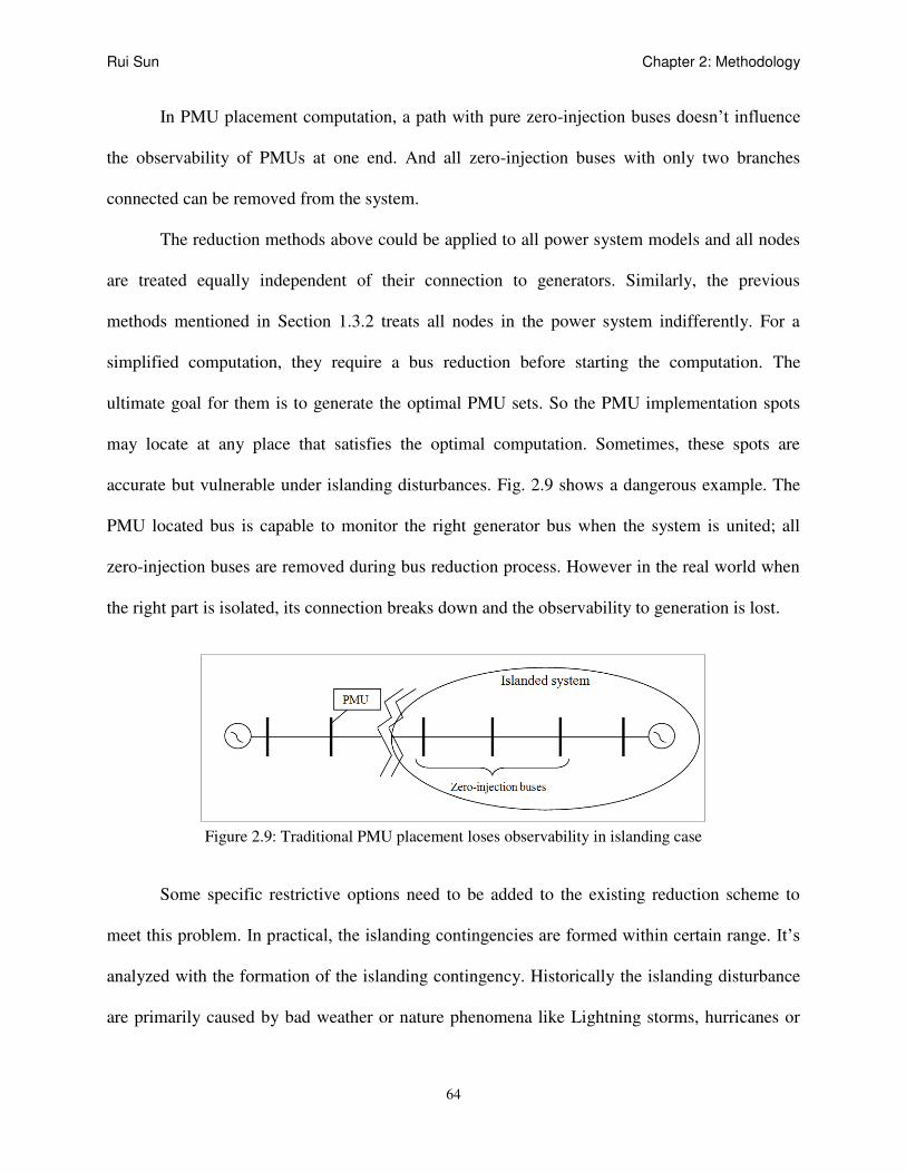
Rui Sun Chapter 2: Methodology
64
In PMU placement computation, a path with pure zero-injection buses doesn’t influence
the observability of PMUs at one end. And all zero-injection buses with only two branches
connected can be removed from the system.
The reduction methods above could be applied to all power system models and all nodes
are treated equally independent of their connection to generators. Similarly, the previous
methods mentioned in Section 1.3.2 treats all nodes in the power system indifferently. For a
simplified computation, they require a bus reduction before starting the computation. The
ultimate goal for them is to generate the optimal PMU sets. So the PMU implementation spots
may locate at any place that satisfies the optimal computation. Sometimes, these spots are
accurate but vulnerable under islanding disturbances. Fig. 2.9 shows a dangerous example. The
PMU located bus is capable to monitor the right generator bus when the system is united; all
zero-injection buses are removed during bus reduction process. However in the real world when
the right part is isolated, its connection breaks down and the observability to generation is lost.
Figure 2.9: Traditional PMU placement loses observability in islanding case
Some specific restrictive options need to be added to the existing reduction scheme to
meet this problem. In practical, the islanding contingencies are formed within certain range. It’s
analyzed with the formation of the islanding contingency. Historically the islanding disturbance
are primarily caused by bad weather or nature phenomena like Lightning storms, hurricanes or

Rui Sun Chapter 2: Methodology
65
extreme cool/hot weather; or cascading breaking down due to hidden failures or equipment
failures. No matter which reason causes the disturbance, the most directly involved buses and
branches sit within a certain region. For the environmental disaster caused cases, the region is
mostly determined by the geographical distances of the buses in the wide area system; for the
cascading failure caused cases, the region is generally decided by the electrical distances.
Finding the optimal PMU set under those restrictions is still our goal. These restrictive options
may include:
1) Certain zero-injection buses are preserved in the system model reduction procedure
because their geographical information in the real world might be essential in the islanding
analysis criteria;
2) To monitor a generator bus, a PMU need to be placed at the near end at the generator
bus rather than a far distance bus. This prevents the cases described in Fig. 2.8.
2.3.5 Binary Integer Programming Algorithm (BIPA)
Traditional PMU placement methods can be divided into two groups: enumeration
method and zero-regressive methods as simulated annealing strategy, genetic algorithm and Tabu
search. Binary integer programming method belongs to the former however, it converts the
placement selection from graphical search to binary and linearized problem, saving enormous
computation time.
To find the minimal PMUs needed, for the system observability problem, the expression
of the method can be written as:
Xf 'min
(2.23)
while bXA
In the equation:

Rui Sun Chapter 2: Methodology
66
A- the system incidence matrix, N by N; it has all its diagonal elements (bus elements)
equaled to 1 which means the bus is connected to the system. For each two buses i, j (i ≠ j)
which have transmission line connected, the corresponding elements in the A matrix Ai,j ,
Aj,i (branch elements) are also 1. Zero-valued element Ax,y refers to the bus X doesn’t
have a connection with bus Y;
X - the PMU placement vector, N by 1; each element representing the number of PMUs
need to be installed in the corresponding bus;
b – the objective vector; N by 1, with each element representing the number of PMUs the
corresponding bus is observed by;
f - the linear inequality constraints vector; it’s an N by 1 vector with each element is
equal to 1.
For optimal PMU placement, the problem turns to:
Xf 'min (2.24)
While bXA Tb 1...11
According to the Theorem 2, in an optimal PMU placement problem, X will only contain
0 or 1. The Problem is purely binary.
Restrictive conditions can be added into the binary problem, and then the problem turns
to:
Xf 'min (2.25)
while bXA
EQEQ bXA AEQ, bEQ are restrictive matrices
When the redundancy is considered, X and b may contain values larger than 1. When this
happens, according to the Theorem 4, b can be separated into several binary vectors which are

Rui Sun Chapter 2: Methodology
67
used to calculate optimal PMU sets after each update of the redundancy requirements. And for b,
there will be a solution X’ as the optimal PMU set. The summation of all X’ vectors will be the
system’s optimal solution to the redundancy problem.
The binary integer programming method separates the redundancy problem into iterations
of optimal problems. For a system redundancy of K:
Stage 1: 1'min Xf TKb 1...11 (2.26)
while 11 bXA Tb 1...111
}{, 11 XiAmO
i
ii 12 Obb
Stage 2: 2'min Xf
while 22 bXA 2b is the optimal requirement for the same system area of b2
}{, 22 XiAmOi
ii 223 Obb
Repeat stage 1 and 2 until all elements in bj = 0
Then j
jXX (2.27)
The binary programming method in solving PMU placement problem has apparent
advantages:
1) Fastness; the time for PMU placement calculation using enumeration method is
extremely large. It is even impossible using enumeration method in large scale system (1000 bus
and more) due to the extreme large number of combinations.
2) Accuracy; the enumeration method is the most accurate method. It can find out all
optimal combinations for any settled requirement. Any other methods, like simulated annealing
strategy, genetic algorithm or Tabu search may not return the optimal solution in one run because
the optimal solution is strongly related with the starting point. However, the binary programming

Rui Sun Chapter 2: Methodology
68
method, due to its simplicity, could solve the large scale system problem and return the optimal
solution obtained from binary level.
3) Simpler to program; all data are converted into binary matrices that any mathematical
software like MATLAB can easily process and use to solve the problem.

69
CHAPTER 3: SIMULATIONS AND RESULTS
3.1 Testing Results on Simulated Islanding Database
The strategies related to the islanding contingency database formation have been tested
on several study systems, including IEEE-14, 30, 57, 118, 300, WECC-128, East coast full-loop
system, etc. The details of the study system models can be found in Appendix B.
3.1.1 Test on System Islanding Detecting Strategy
The system islanding detecting strategy has been tested using multiple systems and
proven to be correct and accurate. Its concept and operating procedures on one specific 8-bus
system example are demonstrated in Section 2.1.3.1. The logic of building up the islanding
detecting strategy is Fig. 3.1:
Figure 3.1: Islanding detecting Strategy Logics

Rui Sun Chapter 3: Simulations and Results
70
The Input for the detecting module contains two parts: one is the study system static data
that describes the system in stationary situation (no dynamic data needed); the other one is the
branch tripping list which includes all tripping conditions need to be tested in the study system.
The program reads in the system data and save it into its working space. Then it searches for the
system incidence matrix (IM). If the IM does not exist, the program will generate the IM from
system branch and bus data. In the next stage, the IM and the branch tripping list are delivered to
the Islanding Judgment module and the IM computation is applied. The outputs generated from
this module include the islanding condition and a brief summary about the size of the generation
and loads inside the island.
3.1.2 Test on the modified enumeration method
The coverage of the modified depth first method has been tested and compared to the
enumeration method. The test results are listed in TABLE 3.1 [29].
TABLE 3.1: COVERAGE TEST FOR DEPTH FIRST METHOD [29]
Test Model (Max.
tripping = 3)
Enumeration Method Modified Depth First Method
Combos
tested
Islanding case
formed
Depth = 2
Combos
tested
Islands
formed Coverage%
IEEE-14 1350 253 999 143 56.52
IEEE-30 11521 1024 3246 245 23.93
IEEE-57 79157 80 6434 20 25
IEEE-118
(up 2 lines) 16110 890 2185 49 5.51
IEEE-300
(up 2 lines) 83845 13786 4073 513 3.72
TABLE 3.1, CONTINUED [29]
Modified Depth First Method
Depth = 3 Depth = 4 Depth = 5
Combo
s tested
Islands
formed
Coverage
%
Combos
tested
Islands
formed
Coverage
%
Combos
tested
Islands
formed
Coverage
%
1343 246 97.2 1350 253 100 - - -

Rui Sun Chapter 3: Simulations and Results
71
8414 701 68.5 11136 963 94.0 11521 1024 100
19246 34 42.5 37219 49 61.3 54882 64 80
3976 97 10.9 5964 182 20.5 8092 286 32.1
7450 1039 7.5 11865 1660 14.0 17048 2760 20.0
The test results illustrate that, while applied in small scale system, the modified
enumeration method (the depth first method) is a good substitute for the enumeration method.
When the system complexity increases, more unreasonable combinations are created through
computation and needed to be disregarded. While taking more time in computation, the
enumeration method could not distinguish them efficiently. On the other hand, the modified
depth first method could concentrate its work on forming islands in the given region, which
prevents recording the unreasonable combinations and saves enormous time. Taking the IEEE-
118 system as an example, when applying the enumeration method, it will take more than 1 day
for computing the islanding combos caused by triple-line tripping. While setting the
observability depth to 4 in modified depth first method, 182 cases are recorded for tripping up to
2 lines and 7,412 cases for tripping up to 3 lines. And the total computation time is 15 minutes.
3.1.3 Tests on DT based Islanding Detection
3.1.3.1 Study System Description
The decision tree algorithm has been carried out on several system models for testing.
The results showed that this method works very well with large scale full loop systems. One of
the major study systems used is a modified MMWG 57,000 Bus Eastern Coast Power Grids
model. The selection of islanding locations is made on the system model within Dominion
Virginia Power (DVP) territory. The Virginia power system territory characteristics have been
introduced in Chapter 1. In this stage, a total number of 190 islanding contingency cases inside
the DVP are selected, generated and recorded, with 300 non-islanding contingency and normal

Rui Sun Chapter 3: Simulations and Results
72
operating cases to form the database (100 normal operation cases; 100 short circuit, 100 rapid
load changing and line tripping cases). The dynamic simulations are done using Python compiled
PSS\E (32.03 version).
As discussed in previous sections, to simulate the practical situations in a wide area
system, only measurements from the highest voltage transmission networks are considered. The
channels of the simulation outputs are the voltage and current phasor (real time load flow)
measurements at the 500kV level buses inside the DVP system.
A) The DVP Area Model Revision of the MMWG 57,000 Bus System
When the MMWG model is modified for simulations, some revisions of the DVP system
are adopted for a better precision. Presently, the most accurate PSS\e models of the DVP area are
six static load flow cases with annual differences of loads, generations and topologies. On the
other hand, the MMWG file, which is a 2008 load version, contains a Dominion transmission
network with simplified topology and dynamic data. Some modifications are adopted between
the MMWG 2008 model and the 2011/ 2012 summer load models.
Revisions include:
1) Using the 2011/2012 DVP system topology to replace the 2008 simplified DVP
subsystem in the MMWG model;
2) Revising the boundary conditions and tie-lines, adding existing tie-lines which were
neglected in the MMWG model;
3) Modifying some system parameters and state variables in the MMWG model;
4) Building up the new dynamic file and conversion options for dynamic simulations.
Tables 3.2 and 3.3 list the differences of the two models at the DVP boundary and bus
numbers:

Rui Sun Chapter 3: Simulations and Results
73
TABLE 3.2: STUDY SYSTEM TIELINE COMPARISON
Tie-line Comparison 2008 MMWG 2011/2012 Summer load
DVP – PJ&M 1 branch 1 branch
DVP – PEPCO 1 branch, simplified 1 branch
DVP – AP 7 branches 10 branches
DVP – AEP 10 branches 10 branches
DVP – CPLE 7 branches, simplified 7 branches
TABLE 3.3: STUDY SYSTEM BUS COMPARISON
2009_Nofull 2011_Summer 2012_Summer
DVP Total 886 Buses 1022 Buses 1032 Buses
23 To Buses 24 To Buses 24 To Buses
DVP Region
500KV 26 31 31
230KV 284 333 341
138KV 12 14 14
115KV 383 448 449
69KV 35 36 36
34.5KV 2 3 3
13.2-26KV 124 157 157
Total 156 163 163
230KV 5 6 6
138KV 1 1 1
115KV 11 9 9
26KV 0 1 1
Generator bus
25KV 2 2 2
24KV 4 4 4
Comparison 22KV 11 12 12
20.5KV 6 6 6
20KV 1 1 1
18KV 23 26 26
14.4KV 8 8 8
13.8KV 77 77 77
13.2KV 7 7 7
The islanding contingency database is created mainly to testify the decision tree
algorithm in islanding assessment. We use the modified 2011 summer case model. The 2012

Rui Sun Chapter 3: Simulations and Results
74
summer case model is used for further research that will be introduced in later sections and next
chapter.
B) The Islanding Database Case Selection
B.1 Islanding Contingency Cases Selection
While selecting the islanded area, we started a thorough search in the DVP territory. The
major concerned possible islanding centers are:
1) The electrical central points in the Dominion system;
2) Areas with large load consumers and relatively vulnerable transmissions;
3) Some regions in the DVP that the connection is radial in topology or geographically
long;
4) Some areas close to the Atlantic coast.
Once the islanding center is located, the program trips one line at the boundary to test the
system isolating condition at every single branch around the boundary, and then move to trip
multiple lines. As we discussed in Chapter 1, the Virginia Power System is analyzed as “some
portions of the transmission system are more heavily loaded than others. This may become the
major weak point to the system in case it splits into parts because the islanded area may face
unbalance generation-load situations. At the same time, The Virginia Power system is along the
east coast of the United States, and is affected by windstorm and thunder storms.” The test
results show one obvious pattern that in many islanding cases, tripping 2 or 3 branches within a
small distance will make certain region in the DVP isolated. This in some extent demonstrates
the radial topology structure in certain part of the DVP system is vulnerable to islanding
situations.

Rui Sun Chapter 3: Simulations and Results
75
Some islanding cases obtained through the islanding detection strategy and the modified
depth method is listed in TABLE 3.4.
TABLE 3.4: SELECTED SIMULATED ISLANDING CASES Case
numbe
r
Lines
Tripping
Combo
Islanded Buses Island
Generatio
n
Island
Loads
Island Gen ID
1 314579-314583 314579, 314591, 314605, 314627, 315136,
315137, 315138
165+j18.3 69.718
+j29.931
315136, 315137, 315138
2 314150-314212
314218-314222
314212, 314215, 314222, 315043, 315044,
315045, 315046, 315047, 315048
606+j74.4 49.771
+j21.913
315043, 315044, 315045,
315046, 315047, 315048
3 314232-314766
314745-314777
314766, 314777, 315177, 315178, 315179,
315180
218-j11.2 19.085
+j3.254
315177, 315178, 315179,
315180
4 314236-314289
314253-314257
314253, 314289, 315067, 315068, 315069,
315070
348+j84.8 31.979
+j11.118
315067, 315068, 315069,
315070
5 314276-314339
314307-314311
314311, 314339, 315083, 315084, 315085,
315086
210+j14.8 40.016
+j8.604
315083, 315084, 315085,
315086
6 314579-314583
314579-314591
314579, 314605, 314627, 315136, 315137,
315138
165+j18.3 41.331
+j20.864
315136, 315137, 315138
7 314579-314583
314611-315139
314579, 314591, 314605, 314627, 315136,
315137, 315138; 315139
275+j9.9 69.718
+j29.931
315136, 315137, 315138,
315139
8 314579-314583
314611-315141
314579, 314591, 314605, 314627, 315136,
315137, 315138; 315141
275+j9.9 69.718
+j29.931
315136, 315137, 315138,
315141
9 314747-314744
314763-314774
314746, 314744, 314748, 314754, 314762,
314763, 314868, 315171, 315170
227-j12.6 71.44
+j24.262
315171, 315170
10 314524-314541
314526-314534
314534, 314541, 314826, 314827, 315115 67.2+j1 11.898
-j1.886
314541, 315115
11 314067-314068
314074-314094
314067, 314070, 314094, 315001, 315002 98-j12.4 151.496
+j44.532
315001, 315002
12 314666-314689
314694-314712
314667, 314671, 314515, 314666, 314700,
314705, 314712, 314348, 314354, 314670,
314680, 314685, 314727, 314728, 314729,
314730, 314731, 314732, 314733, 314734,
314735, 314736, 314737, 314738, 314739,
314740, 314789, 315156, 315165, 315166
147.5-j11.9 78.362
+j21.696
315156, 315165, 315166
The major transmission voltages in the DVP are 500kV, 230kV and 115kV. The DVP
system contains (31) 500kV buses, (349) 230kV buses and (449) 115kV buses. Each voltage
level composes its own transmission network and exchanges power at major substations. The
500kV network is interconnected and considered robust. There are certain parts at 230/115kV
that are radial and easy to be separated. One big composition of the islanding cases occurs at the
low voltage transmission (230/115kV) / distribution (69/35kV) and transformation (13.2 -
22.5kV) networks surrounding certain power plants.
Another point needs to be noticed in the islanding case generation process, is that there
are some cases that lead to islanding contingencies in the simulation however in the real system

Rui Sun Chapter 3: Simulations and Results
76
that they may be prevented by the Dominion’s protection schemes for plants. In the first stage,
we selected 190 cases by tripping up to 3 branches in the study system.
B.2 Non-Islanding Simulation Cases Selection
The non-islanding database is composed of such types of system simulations: normal
operation cases with varying load conditions; short circuit fault cases; rapid load changing cases
and line tripping cases.
The normal operation cases reflect the daily operation conditions of the study system. We
start from the summer peak load model and randomly apply load change at 10% of the load
buses in the DVP. The load change range is within [90%, 110%];
Rapid load change cases occur at the major load buses in the system, a rapid load
increase indicates a jump of the load consumption at the local bus. This is simulated as linear
load increase of an amount of the 100% of the original load within 5 seconds in the PSS\e.
Bus fault cases are carried out at the 230kV and 115kV buses at the DVP. The locations
of the tripping are randomly selected. The fault type selected is the three-phase short circuit. The
faults are considered as permanent faults that last for the rest of the simulation.
Line tripping cases are carried out from 35kV to 500kV at the DVP. We are interested in
500kV line tripping cases in the DVP thus we put several such cases into the database. We also
check the islanding condition to make sure none of the line tripping cases overlaps with the
islanding cases. These trips are considered as permanent faults that last for the whole simulation.
3.1.3.2 Decision Tree Prediction Assessment
The channels of the simulation outputs are the voltage and current phasor (converted
from real time load flow) measurements at the 500kV level buses inside the DVP system. The

Rui Sun Chapter 3: Simulations and Results
77
time stamped simulation results are converted into EXCEL file and used to generate the DTs for
islanding prediction and estimation purpose. In this section, the prediction assessment of each
specific tree is analyzed.
A) The DT for Islanding Detection
The whole islanding database is used to generate this tree. Two methods are used in tree
formation: the 10% test sample method and 10-fold cross validation method [42]. Table 3.2
shows the decision tree prediction success at different tree sizes.
From the fourth column it can be seen that a full-size tree using 10-fold cross validation
method can achieve 98% accuracy for islanding detection basing on the database. In other words,
any islanding case that randomly picked up from the database will have a 98% chance to be
identified correctly using the presented DT. Of course the prediction success rate is largely
relevant to the database size and case selection. The test results have proven that based on a well-
established and updatable database, that the DTs reaching high prediction success indicate the
DT method is capable for online islanding detection and identification. The table also shows the
prediction success for a smaller sized tree with smaller variable importance. For the 10-fold cross
validation DT, if we choose to prune the tree to three or two nodes, the prediction success will
drop to 96.73 and 93.06 percent, which is still fairly high. However, for tree with fewer than 20
nodes, the tree is considered to be simple and having less chance to over-fitting. The prune
process is not recommended at that level.
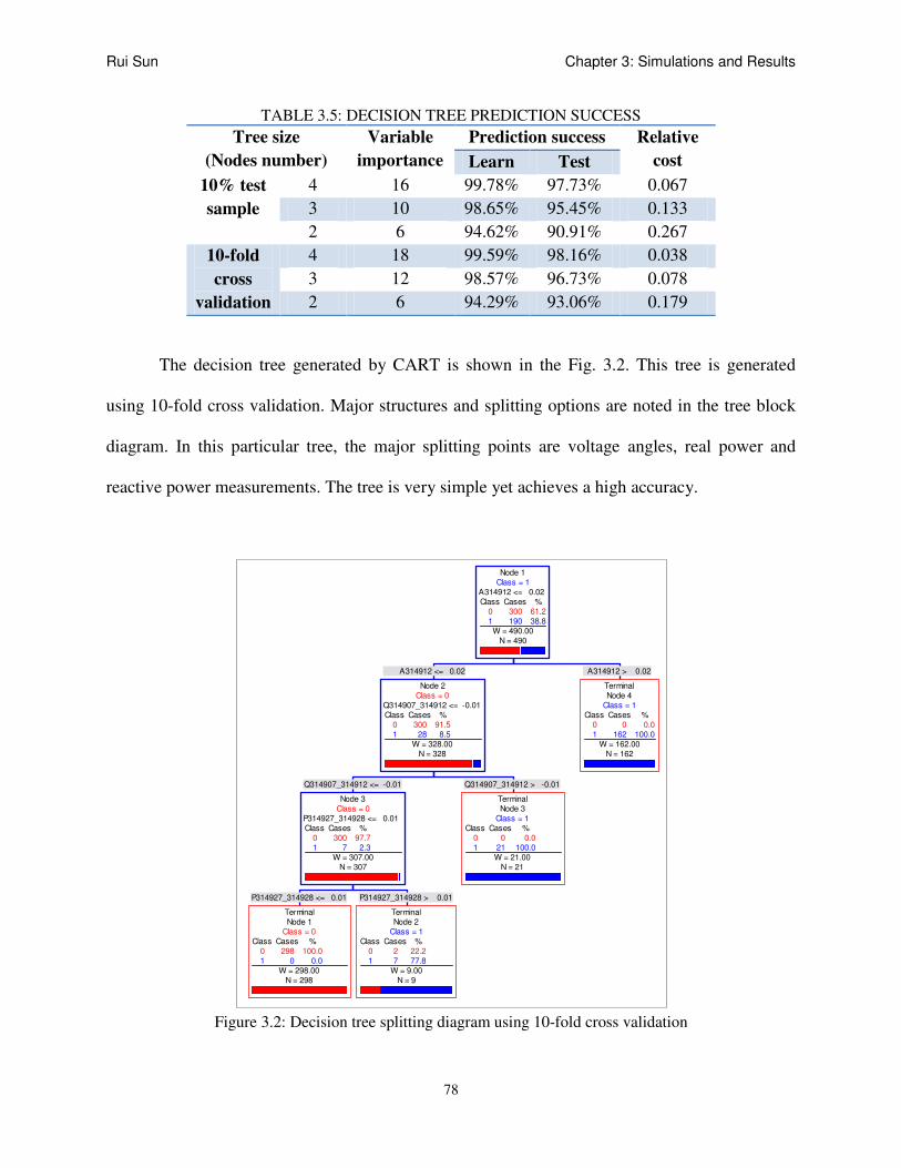
Rui Sun Chapter 3: Simulations and Results
78
TABLE 3.5: DECISION TREE PREDICTION SUCCESS
Tree size
(Nodes number)
Variable
importance
Prediction success Relative
cost Learn Test
10% test
sample
4 16 99.78% 97.73% 0.067
3 10 98.65% 95.45% 0.133
2 6 94.62% 90.91% 0.267
10-fold
cross
validation
4 18 99.59% 98.16% 0.038
3 12 98.57% 96.73% 0.078
2 6 94.29% 93.06% 0.179
The decision tree generated by CART is shown in the Fig. 3.2. This tree is generated
using 10-fold cross validation. Major structures and splitting options are noted in the tree block
diagram. In this particular tree, the major splitting points are voltage angles, real power and
reactive power measurements. The tree is very simple yet achieves a high accuracy.
Figure 3.2: Decision tree splitting diagram using 10-fold cross validation
P314927_314928 <= 0.01
TerminalNode 1
Class = 0Class Cases %
0 298 100.01 0 0.0
W = 298.00N = 298
P314927_314928 > 0.01
TerminalNode 2
Class = 1Class Cases %
0 2 22.21 7 77.8
W = 9.00N = 9
Q314907_314912 <= -0.01
Node 3Class = 0
P314927_314928 <= 0.01Class Cases %
0 300 97.71 7 2.3
W = 307.00N = 307
Q314907_314912 > -0.01
TerminalNode 3
Class = 1Class Cases %
0 0 0.01 21 100.0
W = 21.00N = 21
A314912 <= 0.02
Node 2Class = 0
Q314907_314912 <= -0.01Class Cases %
0 300 91.51 28 8.5
W = 328.00N = 328
A314912 > 0.02
TerminalNode 4
Class = 1Class Cases %
0 0 0.01 162 100.0
W = 162.00N = 162
Node 1Class = 1
A314912 <= 0.02Class Cases %
0 300 61.21 190 38.8W = 490.00
N = 490

Rui Sun Chapter 3: Simulations and Results
79
The DTs are also useful for the PMU placement assessment. When forming the trees, the
primary split variables are referred to as having the most effluence to the prediction accuracy.
The places where these variables are measured are also the critical PMU locations for
implementation of islanding detection application. In this test, all state variables are from 30
locations at the 500kV network; among them are the major substations with PMUs installed. The
measurements at those locations show exactly what the PMUs may see when an island form in a
lower voltage area and how this island would influence the major 500kV transmission network.
For a tree using 18 system variables in determination, the variables may just come from 4
different locations.
B) Islanding Behavior Groups
A successive study of the islanding characteristics of the 190 islanding cases was carried
out. Major islanding cases were run for 20 seconds and the angle variables of the involved
generators were tracked. Three types of islanding categories were obtained
B.1 Category 1:
- Machines in the islands are angle coherent;
- The islanded area remains stable;
- The islanded machine angles have a relatively larger oscillation in a different direction
compared with the main grids;
- In some cases, the islanded area is connected with tie-lines outside the Virginia area.
Although a Virginia region is physically islanded it still receives power delivered from outside
the area. (This is due to: the islanding detecting strategy is applied within the partial incidence
matrix of the DVP, thus some of the boundary tie-lines are kept in some cases. However, these

Rui Sun Chapter 3: Simulations and Results
80
cases are still thought islands – not a physical but an electrical island for which the utility losses
the control of the island.)
Figure 3.3: Machine angles oscillation of category 1 cases
B.2 Category 2:
- Machines in the islands are angle coherent;
- The islanded area lost stability after the contingency;
0 2 4 6 8 10 12 14 16 18 20-20
-15
-10
-5
0
5
Time (second)
Angle
(degre
e)
ANGL315136[1ROSEMG1 13.800]G1
ANGL315137[1ROSEMS1 13.800]S1
ANGL315138[1ROSEMG2 13.800]G2
0 1 2 3 4 5 6 7 8 9 10-40
-30
-20
-10
0
10
20
30
40
Time (second)
Angle
(degre
e)
ANGL315136[1ROSEMG1 13.800]G1
ANGL315137[1ROSEMS1 13.800]S1
ANGL315138[1ROSEMG2 13.800]G2

Rui Sun Chapter 3: Simulations and Results
81
- The islanded machine angles go up because of a mismatch between loads and
generation; the angles in the main grid go to the opposite direction. Protection actions are needed.
Figure 3.4: Machine angles oscillation of category 2 cases
B.3 Category 3:
- Machines in the islands are angle coherent;
0 0.5 1 1.5 2 2.5 3 3.5 4 4.5 5-20
0
20
40
60
80
100
120
140
160
180
Time (second)
Angle
(degre
e)
ANGL315067[1DARBY 1 13.800]1
ANGL315068[1DARBY 2 13.800]2
ANGL315069[1DARBY 3 13.800]3
ANGL315070[1DARBY 4 13.800]4
0 1 2 3 4 5 6 7 8 9 10
0
50
100
150
200
Time (second)
An
gle
(d
eg
ree
)
ANGL315177[1SANNAG1 13.800]G1
ANGL315179[1SANNAG2 13.800]G2
ANGL315178[1SANNAS1 13.800]S1
ANGL315180[1SANNAS2 13.800]S2

Rui Sun Chapter 3: Simulations and Results
82
- The islanded area remains stable after the contingency and the islanded machine angles
go along with the main grid.
- Some machines not included in the island but near the boundary are influenced more by
the contingency. Sometimes the generators related to the islanded area lost stability.
- In some cases, the islanded area is connected with tie lines outside the Virginia area.
Figure 3.5: Machine angles oscillation of category 3 cases
0 2 4 6 8 10 12 14 16 18 200
2
4
6
8
10
12
14
16
18
20
Time (second)
Angle
(degre
e)
ANGL315171[1BREMO 4 18.000]4
ANGL315170[1BREMO 3 13.800]3
0 1 2 3 4 5 6 7 8 9 10-20
-15
-10
-5
0
5
10
15
20
25
Time (second)
Angle
(degre
e)
ANGL315171[1BREMO 4 18.000]4
ANGL315170[1BREMO 3 13.800]3

Rui Sun Chapter 3: Simulations and Results
83
C) The DT for Other Islanding Issues
As it was stated previously, the islanding contingency database is created mainly to test
the decision tree algorithm in islanding detection. While the DT algorithm can achieve more
functions including islanding location estimation, islanding stability assessment or islanding area
estimation. Tests on these functions are made using different islanding databases, corresponding
decision trees are obtained and analyzed. A brief introduction of the specialized islanding
database used for such purposes as well as for the islanding severity index usage is given in
Section 3.2. The detailed database introduction and DT analysis are given in Chapter Four.

Rui Sun Chapter 3: Simulations and Results
84
3.2 Testing Results on Islanding Severity Index
The ISI is a proposed method for ranking the system transient behavior and severity level
of islanding contingencies. The ISI works as an additional tool to assist the DTs in islanding
severity determination. The method itself is a very useful tool in power system islanding analysis.
It offers a way to qualify and quantify the islanding severity for any islanding scenarios proposed
in a study system both offline and online. In the offline analysis, it can help judging the
underlying weakness points of a study system under unbalanced power condition.
A successive islanding severity test of the (190+300) islanding database was carried out
on selected islanding cases based on the islanding groups analysis. The long-term and instant ISI
values were calculated via equation (2.20) and (2.21). Table 3.5 shows 10 typical islanding
contingency cases taken from the database. According to the computation, category 2 islanding
cases have relatively larger ISI instant and long-term values than the category 1 and 3 cases.
Islanding case with a higher instant ISI value show larger angle oscillations; while it doesn’t
necessarily mean it has a higher long-term ISI value which is related to the generators’ inertia
and have effect to their power re-dispatch characteristic. Those Island cases with huge generation
have correspondingly much larger long-term ISI values however a large ISI value does not
indicate the machines in the island will lose stability. There are also some meter islanding cases
in the system; case 7-10 all have inter-area tie-lines connected with the islanded area. Although
in these cases they have relatively high instant and long-term ISI values, the islanded areas are
still stable, however the influences to the system is more severe than category 1 cases, which are
also shown as the more severe angle oscillations at boundary generators.

Rui Sun Chapter 3: Simulations and Results
85
TABLE 3.6: ISLANDING SEVERITY INDEX ANALYSIS
Case
#
Island
Generation
Mismatches Inertia
Combo
Cate
gory
ISI_
Instant
ISI_
long-term P Q
1 165+j18.3 -63.42 8.469 15.3 1 0.384 4.145
2 3030+j397.2 3030 397.2 52.92 2 1 57.256
3 1744-j254.2 -429.2 -385.8 20.22 1 0.246 21.226
4 606+j74.4 556.23 52.487 27.54 2 0.918 20.197
5 348+j84.8 316.02 73.682 26 2 0.908 12.155
6 275+j9.9 46.582 0.069 15.3 1 0.169 3.0446
7 227-j12.6 92.111 -32.85 6.82 3 0.406 13.506
8 227-j12.6 84.76 -36.06 6.82 3 0.373 12.428
9 147.5-j11.9 95.738 -53.60 6.232 3 0.649 15.362
10 147.5-j11.9 118.67 -47.22 6.232 3 0.805 19.042
For the major ISI analysis, a different set of data is used to compose the database. We
narrowed our simulations into one smaller region which is considered to be the most potential
islanding location in the DVP. A series of islanding cases are formed on the selected locations,
and the islanding severity index is computed. A curve-fitting approach is used to simulate the
frequency oscillations of the isolated area to help demonstrate how the index ranks the severity
of the event. All contingency dynamic simulations are done using Python compiled PSS\E (32.03
version).
3.2.1 The Creation of the Islanding Database for ISI
The creation process includes four stages:
1) Based on the geographical distribution of the transmission network around selected
islanding location, the system one-line diagram is made;
2) The one line diagram of the selected area is separated into four partitions (0-3) for a
convenient load calculation. The partition determination is based on the system topology
characteristics and load condition;

Rui Sun Chapter 3: Simulations and Results
86
3) The determination of the isolated area is first performed based on the geographic map
in Fig. 3.6 and 3.7. The isolated area analysis starts from the selected sub-station and radiates
outwards. For each of the two directions, the transmission lines come out of the station circles
with increasing radius which indicates a growth of the possible islanding areas along the
transmission paths. The potential islanding regions are labeled by the cut-off locations using red
and purple dotted lines.
Figure 3.6: Geographic diagram around the selected area
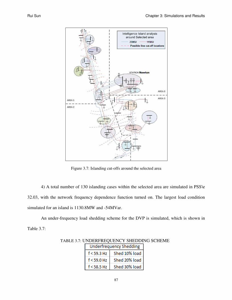
Rui Sun Chapter 3: Simulations and Results
87
Figure 3.7: Islanding cut-offs around the selected area
4) A total number of 130 islanding cases within the selected area are simulated in PSS\e
32.03, with the network frequency dependence function turned on. The largest load condition
simulated for an island is 1130.8MW and -54MVar.
An under-frequency load shedding scheme for the DVP is simulated, which is shown in
Table 3.7:
TABLE 3.7: UNDERFREQUENCY SHEDDING SCHEME

Rui Sun Chapter 3: Simulations and Results
88
A maximum of 30% load will be shed during the protection operation. The time for
communication delay and relay/breaker operation for each shedding is 0.2833 second. If after the
three stages the frequency of the island is still below 58.5Hz the whole isolated area will be
tripped, in other words, the island is considered unstable.
In 130 cases, without load shedding, there are 68 cases with steady frequency over 59.3
Hz and 23 cases below 58.5 Hz. For any case when the frequency drops below 58.5 Hz, a load
shedding protection will be applied. For 75 cases, 17 cases apply 10% load shedding only, 30
cases apply 20% load shedding and 28 cases apply 30% load shedding. After applying the load
shedding scheme, there are 4 cases with frequency still below 58.5 Hz.
3.2.2 ISI Computation and Analysis
Using the equations derived from (2.20) and (2.21), the index values before load
shedding and right after the shedding are computed differently as:
GEN
iniloa dsiniGEN
H
PPinilongtermISI
__)(_
iniGEN
iniloa dsiniGEN
P
PPiniinstentISI
_
__)(_
(3.1)
And:
GEN
ploa dssheddingGEN
H
PPpostlongtermISI
_@)(_
sheddingGEN
ploa dssheddingGEN
P
PPpostinstentISI
@
_@)(_
(3.2)

Rui Sun Chapter 3: Simulations and Results
89
TABLE 3.8: ISI FOR THE STUDY SYSTEM Case
#
P_ld
(ini)
P_ld
(post)
Freq. w/o
shed
Final
Freq.
ISI_Lo
ng(ini)
ISI_Lo
ng(post)
ISI_Insta
nt(ini)
ISI_Insta
nt(post)
1 1139.7 797.79 51.041 58.577 60.96 19.60 1.175 0.199
2 1039.4 727.58 58.256 58.860 51.03 19.22 0.984 0.211
3 1039.4 727.58 58.289 58.805 51.03 19.57 0.984 0.214
4 995.4 696.78 58.419 58.930 46.67 18.02 0.900 0.207
5 916.6 733.28 58.658 59.109 38.87 8.42 0.749 0.104
6 877.8 702.24 58.769 59.220 35.03 8.66 0.675 0.111
7 799 639.2 59.008 59.430 27.23 15.83 0.525 0.200
8 715.4 643.86 59.259 59.424 18.95 7.87 0.365 0.110
9 665.4 598.86 59.418 59.573 14.00 12.46 0.270 0.174
10 1112.3 778.61 27.811 31.571 58.25 51.60 1.123 0.401
11 1012 708.4 31.221 43.118 48.32 48.59 0.931 0.409
12 1012 708.4 58.368 58.886 48.32 18.11 0.931 0.205
13 968 677.6 58.498 59.007 43.96 18.59 0.847 0.217
14 889.2 711.36 58.738 59.187 36.16 8.29 0.697 0.105
15 850.4 680.32 58.849 59.295 32.32 16.41 0.623 0.196
16 771.6 617.28 59.089 59.505 24.51 15.51 0.473 0.202
17 688 619.2 59.340 59.506 16.24 12.90 0.313 0.174
18 638 638 59.500 59.500 11.29 11.29 0.218 0.218
19 1071.2 749.84 30.283 45.788 54.18 47.02 1.044 0.388
20 986.9 690.83 43.980 58.226 45.83 38.06 0.883 0.358
21 886.6 709.28 58.709 59.249 35.90 8.72 0.692 0.110
22 886.6 709.28 58.739 59.202 35.90 16.77 0.692 0.193
23 842.6 674.08 58.869 59.318 31.54 16.32 0.608 0.196
24 763.8 611.04 59.109 59.528 23.74 15.40 0.458 0.203
25 725 652.5 59.222 59.405 19.90 13.58 0.384 0.174
26 646.2 581.58 59.462 59.631 12.10 7.67 0.233 0.118
27 562.6 562.6 59.714 59.714 3.82 3.82 0.074 0.074
28 512.6 512.6 59.870 59.870 1.13 1.13 0.022 0.022
29 1158.4 810.88 46.612 58.565 62.81 21.51 1.211 0.211
30 1019.5 713.65 58.221 58.895 49.06 18.38 0.946 0.206
…
93 220.8 220.8 61.799 61.799 30.02 30.02 0.579 0.579
94 1006.8 704.76 58.237 58.978 47.80 18.24 0.921 0.207
95 867.9 694.32 58.672 59.277 34.05 8.61 0.656 0.111
96 851.4 681.12 58.762 59.322 32.42 8.53 0.625 0.112
97 751.1 600.88 59.117 59.596 22.49 15.56 0.433 0.207
98 666.8 600.12 59.313 59.615 14.14 8.17 0.273 0.121
99 566.5 566.5 59.675 59.675 4.21 4.21 0.081 0.081
100 566.5 566.5 59.698 59.698 4.21 4.21 0.081 0.081
101 522.5 522.5 59.831 59.831 0.15 0.15 0.003 0.003
102 443.7 443.7 60.015 60.015 7.95 7.95 0.153 0.153
103 404.9 404.9 60.122 60.122 11.79 11.79 0.227 0.227
104 326.1 326.1 60.708 60.708 19.59 19.59 0.378 0.378
105 242.5 242.5 61.100 61.100 27.87 27.87 0.537 0.537
106 192.5 192.5 64.779 64.779 32.82 32.82 0.633 0.633
107 1006.8 704.76 58.237 58.978 47.80 18.23 0.921 0.207
108 867.9 694.32 58.672 59.277 34.05 8.60 0.656 0.111
109 851.4 681.12 58.762 59.322 32.42 8.53 0.625 0.112
110 751.1 600.88 59.117 59.596 22.49 15.56 0.433 0.207
111 666.8 600.12 59.313 59.615 14.14 8.16 0.273 0.121
112 566.5 566.5 59.675 59.675 4.21 4.21 0.081 0.081
113 566.5 566.5 59.698 59.698 4.21 4.21 0.081 0.081
114 522.5 522.5 59.831 59.831 0.15 0.15 0.003 0.003
115 443.7 443.7 60.015 60.015 7.95 7.95 0.153 0.153
116 404.9 404.9 60.122 60.122 11.79 11.79 0.227 0.227
117 326.1 326.1 60.708 60.708 19.59 19.59 0.378 0.378
118 242.5 242.5 61.100 61.100 27.87 27.87 0.537 0.537
119 192.5 192.5 64.781 64.781 32.82 32.82 0.633 0.633
120 926.1 648.27 58.482 59.183 39.81 18.28 0.767 0.222
…

Rui Sun Chapter 3: Simulations and Results
90
The analysis starts from the comparison between the scenarios with and without a load
shedding scheme. The 4th
and 5th
column in Table 3.7 are the frequencies of the island with and
without load shedding after 20 seconds. Under-frequency and over-frequency cases are shown in
bold in first column. The load shedding action effectively improves the stability of the islands.
By applying the load shedding scheme, the number of unstable islanding cases decreases from 23
to 4, considering the system has come back to steady state for most stable cases at 20 seconds
after the contingency. This change is precisely demonstrated by the values of the long-term index.
For the selected area, a severe threshold at 38 can be set for long term ISI, all cases with higher
long-term values are proved to be unstable. With load shedding, most large long-term values
have turned small, while the unstable ones remain large. The results also show that for over-
generating cases (106 and 119), the long-term index does not give a significant difference. They
may have relatively large values but still within the threshold.
The instant ISI focuses mostly on the transient behaviors during the first couple of
seconds after the contingency. A larger index value refers to a more intense oscillation and
transient behavior. In most cases, the contingencies with higher long term influence will have
more severe transient behaviors. The instant index value may shift due to any change in the
system structure or load/generation condition. The initial instant index values express a
coherency between the long-term index values but the instant index could recognize over-
generating cases with relatively high values. For the over-generating cases, the frequency will
finally go back close to 60Hz due to the governor system however their larger transient
behaviors needs more time for damping. This is also shown in the graphs. It is not safe to assume
that a long-term good case is absolutely moderate in transient; these are two independent indices.

Rui Sun Chapter 3: Simulations and Results
91
3.2.3 Curve fitting comparison and analysis
An approach to model the transient frequency oscillation of each islanding event using
curve fitting program is described in this section. The fitted curve model is determined as:
CewtAftfbt
ininew )sin()( (3.3)
Where:
A – the largest frequency oscillation magnitude (the magnitude of the first oscillation
cycle most time);
b – the oscillation decay speed;
C – the frequency deviation after 20 seconds;
w – the oscillation natural frequency.
The values of the parameters A, b and C reflect the degree the frequency oscillation as
well as the severity of the contingency. For a severe case, the A value tends to be larger and b
smaller; while C could be larger in its absolute value. For the long-term stable islands in this
study, the value of C is expected to be within (-1.5, 1.8).
Selected fitting curve samples are listed in Fig. 3.8 and 3.9:

Rui Sun Chapter 3: Simulations and Results
92
Figure 3.8: Selected fitting curve samples
2 4 6 8 10 12 14 16 18 20-10
-8
-6
-4
-2
0
2
4x 10
-3
T (second)
Fre
quency o
scill
ation (
p.u
.)
Frequency Transients
Fit curve 1
Case 37: no load shedding performed
a = -1.465464662b = 0.930759509 c = -0.3926 w = 1.582542226theta = -2.384783159
2 4 6 8 10 12 14 16 18 20-16
-14
-12
-10
-8
-6
-4
-2
0
2
4x 10
-3
T (second)
Fre
quency T
ransie
nt (p
.u.)
Frequency Transients
Fit curve 1
Case 98:10% load shedding performed
a = -3.444017003 b = 0.954727762c = -0.392w = 1.670178428 theta = -2.066758849
2 4 6 8 10 12 14 16 18 20-0.03
-0.025
-0.02
-0.015
-0.01
-0.005
0
0.005
T (second)
Fre
quency O
scill
ation (
p.u
.)
Frequency Transients
Fit curve 1
Case 120:30% load shedding performed
a = -6.416639889b = 1.035856736c = -0.8203w = 1.740684707theta = -2.174563335

Rui Sun Chapter 3: Simulations and Results
93
Figure 3.9: Selected fitting curve samples (cont.)
Case 37 in Fig 3.8 is stable and does not need load shedding; cases 98 needs 10% load
shedding and case 120 needs 30% load shedding. Case 119 is an over-generating case stable in
the long term. Case 10 is unstable and the island collapses after 20 seconds.
2 4 6 8 10 12 14 16 18 20-0.02
0
0.02
0.04
0.06
0.08
0.1
T (second)
Fre
quency o
scill
ation (
p.u
.)
Frequency Transients
Fit curve 1
Case 119:Over generated
a = -48.6218459b = 0.131233979c = 3.536w = 0.025241218theta = 3.03389589
2 4 6 8 10 12 14 16 18 20-0.5
-0.45
-0.4
-0.35
-0.3
-0.25
-0.2
-0.15
-0.1
-0.05
0
T (second)
Fre
quency o
scill
ation (
p.u
.)
Frequency Transients
Fit curve 1
Case 10:Island collapsed with load shedding
a = 3941.075973b = 0.257462624c = -26.0273w = 0.002916204theta = 0.004113125

Rui Sun Chapter 3: Simulations and Results
94
TABLE 3.9: ISI WITH CURVE FITTING PARAMETERS Case
#
ISI_Lo
ng(ini)
ISI_Lo
ng(post)
ISI_Inst
ant(ini)
ISI_Insta
nt(post)
A b C
(in Hz)
w
(in pi)
1 60.96 19.60 1.175 0.199 -6.4724 1.0086 -1.4246 1.8615
2 51.03 19.22 0.984 0.211 -5.7894 0.9864 -1.1418 1.8348
3 51.03 19.57 0.984 0.214 -5.5248 1.0205 -1.1992 1.8314
4 46.67 18.02 0.900 0.207 -5.1945 1.0043 -1.0745 1.8278
5 38.87 8.42 0.749 0.104 -4.5058 0.9962 -0.8971 1.8429
6 35.03 8.66 0.675 0.111 -4.3031 0.9742 -0.786 1.8283
7 27.23 15.83 0.525 0.200 -3.4601 0.9030 -0.5776 1.8216
8 18.95 7.87 0.365 0.110 -2.5504 0.9357 -0.5833 1.7635
9 14.00 12.46 0.270 0.174 -1.9560 0.8435 -0.4347 1.7337
10 58.25 51.60 1.123 0.401 3941.1 0.2575 -26.027 0.0029
11 48.32 48.59 0.931 0.409 14597.8 0.8184 -11.082 0.0033
12 48.32 18.11 0.931 0.205 -5.3338 1.0113 -1.1187 1.8306
13 43.96 18.59 0.847 0.217 -5.0104 0.9962 -0.998 1.8268
14 36.16 8.29 0.697 0.105 -4.2987 0.9838 -0.8192 1.8422
15 32.32 16.41 0.623 0.196 -4.0765 0.9580 -0.7113 1.8269
16 24.51 15.51 0.473 0.202 -3.1990 0.8640 -0.5028 1.8038
17 16.24 12.90 0.313 0.174 -2.2869 0.8992 -0.5012 1.7569
18 11.29 11.29 0.218 0.218 -1.8212 0.9657 -0.5068 1.6094
19 54.18 47.02 1.044 0.388 9221.4 0.8480 -9.58 0.0043
20 45.83 38.06 0.883 0.358 -10.129 1.2025 -1.7784 1.4685
21 35.90 8.72 0.692 0.110 -5.2010 0.9977 -0.7556 1.7716
22 35.90 16.77 0.692 0.193 -4.4235 0.9816 -0.8034 1.8305
23 31.54 16.32 0.608 0.196 -4.0397 0.9527 -0.6883 1.8256
24 23.74 15.40 0.458 0.203 -3.1564 0.8545 -0.4801 1.7977
25 19.90 13.58 0.384 0.174 -2.7574 0.9407 -0.6015 1.7633
26 12.10 7.67 0.233 0.118 -1.8321 0.7883 -0.3768 1.7050
27 3.82 3.82 0.074 0.074 -1.2416 0.9649 -0.2927 1.4909
28 1.13 1.13 0.022 0.022 -1.3698 1.1929 -0.1351 0.9965
29 62.81 21.51 1.211 0.211 -6.7719 0.9810 -1.4352 1.8592
30 49.06 18.38 0.946 0.206 -6.0115 1.0138 -1.1083 1.8371
31 47.43 18.19 0.914 0.207 -5.7578 1.0035 -1.0642 1.8344
32 37.50 17.52 0.723 0.219 -5.0193 0.9784 -0.7998 1.7934
33 29.15 8.66 0.562 0.118 -5.0637 1.0043 -0.5866 1.7688
34 19.22 15.26 0.370 0.211 -4.1948 0.9278 -0.3203 1.6816
35 19.22 13.73 0.370 0.177 -2.7141 0.9296 -0.5782 1.7613
36 14.86 13.51 0.286 0.184 -2.2862 0.8752 -0.454 1.7456
37 7.06 7.06 0.136 0.136 -1.4655 0.9308 -0.3926 1.5825
38 3.22 3.22 0.062 0.062 -1.2422 0.9226 -0.2775 1.4664
39 4.58 4.58 0.088 0.088 -0.3886 1.0333 -0.0597 1.4918
40 12.86 12.86 0.248 0.248 0.7113 0.2139 0.2299 0.3186
…
93 30.02 30.02 0.579 0.579 -65.941 0.1175 -1.0713 0.0257
94 47.80 18.24 0.921 0.207 -6.5416 1.0099 -1.0233 1.7802
95 34.05 8.61 0.656 0.111 -5.0126 0.9899 -0.7273 1.8392
96 32.42 8.53 0.625 0.112 -4.7248 0.9746 -0.683 1.8308
97 22.49 15.56 0.433 0.207 -4.0524 0.9215 -0.4112 1.7363
98 14.14 8.17 0.273 0.121 -3.4440 0.9547 -0.392 1.6702
99 4.21 4.21 0.081 0.081 -1.8095 0.8451 -0.3341 1.3637
100 4.21 4.21 0.081 0.081 -1.2848 0.9092 -0.3086 1.5343
101 0.15 0.15 0.003 0.003 -1.0613 0.9633 -0.1759 1.3622
102 7.95 7.95 0.153 0.153 0.0059 0.3976 0.0157 0.9201
103 11.79 11.79 0.227 0.227 0.3813 0.2144 0.1221 0.3246
104 19.59 19.59 0.378 0.378 -2.0705 0.1991 0.7274 0.3237
105 27.87 27.87 0.537 0.537 -4.2818 0.1114 1.3733 0.2336
106 32.82 32.82 0.633 0.633 -46.501 0.1297 3.478 0.0265
107 47.80 18.23 0.921 0.207 -6.5377 1.0098 -1.0235 1.7805
108 34.05 8.60 0.656 0.111 -5.0118 0.9900 -0.7275 1.8392
109 32.42 8.53 0.625 0.112 -4.7229 0.9746 -0.6831 1.8309
110 22.49 15.56 0.433 0.207 -4.0489 0.9213 -0.4113 1.7365

Rui Sun Chapter 3: Simulations and Results
95
111 14.14 8.16 0.273 0.121 -3.4413 0.9547 -0.3922 1.6703
112 4.21 4.21 0.081 0.081 -1.8116 0.8463 -0.3341 1.3634
113 4.21 4.21 0.081 0.081 -1.2845 0.9096 -0.3086 1.5345
114 0.15 0.15 0.003 0.003 -1.0608 0.9638 -0.1759 1.3624
115 7.95 7.95 0.153 0.153 0.0067 0.4133 0.0157 0.9088
116 11.79 11.79 0.227 0.227 0.3826 0.2146 0.1223 0.3245
117 19.59 19.59 0.378 0.378 -2.0715 0.1992 0.7276 0.3236
118 27.87 27.87 0.537 0.537 -4.2880 0.1114 1.3724 0.2334
119 32.82 32.82 0.633 0.633 -48.622 0.1312 3.536 0.0252
120 39.81 18.28 0.767 0.222 -6.4166 1.0359 -0.8203 1.7407
…
The oscillation’s curve fitting parameters demonstrate the effectiveness of the instant
index. As stated before, the values of the parameters A, b and C reflect the range of the
frequency oscillation as well as the severity of the contingency. Table 3.9 shows the most severe
cases (10, 11 and 19) have quite large A values according to the fitting configuration. And so do
the over-generating cases. The less severe cases have larger b indicating a faster damping. The
least severe cases have the relatively smallest ISI values.
3.2.4 Adapted real time ISI computation and analysis
The ISI values can be computed using saved system parameters and estimated data. In
other words, this index is very useful for researchers to study the islanding response of certain
system. The ISI could update with real-time measurements and system status to reflect a more
accurate qualification of islanding cases.
According to the Equation (2.20) in Chapter 2, the islanding severity index value has a
consistency with K times the time derivative of the generator angle velocity at the isolated areas.
The time derivative of the generator angle velocity of the selected station at the selected time are
recorded and listed in Table 3.10.

Rui Sun Chapter 3: Simulations and Results
96
TABLE 3.10: REAL TIME ISI COMPUTATION
Case
#
ISI_Lo
ng(ini)
ISI_Lo
ng(post)
ISI_Inst
ant(ini)
ISI_Insta
nt(post)
2*d(theta)/d2t
ini Ld_shed t = 5 t = 10
1 60.96 19.60 1.175 0.199 11.303 1.416 0.186 0.005
2 51.03 19.22 0.984 0.211 9.764 0.740 0.169 0.002
3 51.03 19.57 0.984 0.214 9.034 0.680 0.138 0.002
4 46.67 18.02 0.900 0.207 8.464 0.075 0.128 0.006
5 38.87 8.42 0.749 0.104 7.265 0.108 0.105 0.005
6 35.03 8.66 0.675 0.111 6.740 0.169 0.099 0.006
7 27.23 15.83 0.525 0.200 5.505 0.466 0.084 0.001
8 18.95 7.87 0.365 0.110 4.138 0.024 0.070 0.001
9 14.00 12.46 0.270 0.174 3.799 0.345 0.069 0.003
10 58.25 51.60 1.123 0.401 15.792 5.545 3.226 3.198
11 48.32 48.59 0.931 0.409 13.536 4.180 1.766 1.681
12 48.32 18.11 0.931 0.205 8.716 0.094 0.132 0.001
13 43.96 18.59 0.847 0.217 8.142 0.138 0.122 0.004
14 36.16 8.29 0.697 0.105 6.954 0.189 0.100 0.004
15 32.32 16.41 0.623 0.196 6.412 1.115 0.096 0.001
16 24.51 15.51 0.473 0.202 5.186 0.117 0.085 0.004
17 16.24 12.90 0.313 0.174 3.816 0.697 0.066 0.003
18 11.29 11.29 0.218 0.218 3.467 0.054 0.002
19 54.18 47.02 1.044 0.388 14.184 4.574 1.366 1.336
20 45.83 38.06 0.883 0.358 11.870 2.409 0.153 0.000
21 35.90 8.72 0.692 0.110 7.592 0.040 0.124 0.002
22 35.90 16.77 0.692 0.193 6.852 1.576 0.101 0.001
23 31.54 16.32 0.608 0.196 6.266 1.034 0.092 0.004
24 23.74 15.40 0.458 0.203 5.012 0.025 0.085 0.005
25 19.90 13.58 0.384 0.174 4.482 1.247 0.078 0.006
26 12.10 7.67 0.233 0.118 3.177 1.028 0.073 0.003
27 3.82 3.82 0.074 0.074 1.767 0.029 0.004
28 1.13 1.13 0.022 0.022 1.426 0.010 0.003
29 62.81 21.51 1.211 0.211 11.303 1.416 0.186 0.005
30 49.06 18.38 0.946 0.206 9.764 0.740 0.169 0.002
…
101 0.15 0.15 0.003 0.003 2.857 0.061 0.001
102 7.95 7.95 0.153 0.153 2.138 0.042 0.004
103 11.79 11.79 0.227 0.227 1.489 0.027 0.002
104 19.59 19.59 0.378 0.378 0.151 0.000 0.000
105 27.87 27.87 0.537 0.537 0.363 0.001 0.037
106 32.82 32.82 0.633 0.633 1.773 0.083 0.216
107 47.80 18.23 0.921 0.207 3.271 0.508 0.366
108 34.05 8.60 0.656 0.111 3.647 1.093 0.196
109 32.42 8.53 0.625 0.112 9.994 0.209 0.178 0.005
110 22.49 15.56 0.433 0.207 7.532 0.235 0.111 0.004
111 14.14 8.16 0.273 0.121 7.138 0.389 0.109 0.005
112 4.21 4.21 0.081 0.081 5.475 0.015 0.087 0.004
113 4.21 4.21 0.081 0.081 4.618 0.827 0.066 0.003
114 0.15 0.15 0.003 0.003 2.856 0.060 0.002
115 7.95 7.95 0.153 0.153 2.137 0.042 0.002
116 11.79 11.79 0.227 0.227 1.488 0.026 0.004
117 19.59 19.59 0.378 0.378 0.150 0.001 0.000
118 27.87 27.87 0.537 0.537 0.364 0.001 0.036
119 32.82 32.82 0.633 0.633 1.774 0.082 0.214
120 39.81 18.28 0.767 0.222 3.272 0.508 0.364
…
In the simulation, only one island is created each time and one station is involved. So the
relation could be simplified as between the original instant index value and the time derivative of

Rui Sun Chapter 3: Simulations and Results
97
the angle velocity. The test results have shown this consistency, especially at the time when the
island forms. With the increase of time, the frequency oscillation decays, along with the decrease
of the time derivative variable. For the unstable cases (10, 11 and 19), the time derivatives keep
high even after 10 seconds, while in other cases, the values have already decayed close to 0. The
time derivative could be used to compute the real-time ISI for both long-term and instantaneous
indices, respectively.

Rui Sun Chapter 3: Simulations and Results
98
3.3 Results on the Optimal PMU Placement Using BIPA
3.3.1 Optimal PMU Placement
The proposed method is tested on IEEE-14/30/39/57/118/300 BUS and WECC-128 BUS
system models.
TABLE 3.11: BUS REDUCTION USING MODIFIED SCHEME
System
models
Bus Reduction
Original
scale
Virtual bus
eliminated
Zero-injection
bus eliminated
Final
scale
IEEE-14 14×14 1 1 12×12
IEEE-30 30×30 0 2 28×28
IEEE-39 39×39 9 2 28×28
IEEE-57 57×57 0 7 50×50
IEEE-118 118×118 0 3 115×115
WECC-128 128×128 29 15 84×84
IEEE-300 300×300 24 22 254×254
Table 3.11 shows the system model scales before and after applying the modified bus
reduction scheme. Due to the restrictive options, only limited number of buses is reduced.
For the purpose of monitoring the whole system’s operating situation without losing
information of the generations in an isolated system, placing PMUs at buses which have direct
coverage of the generators is one of the priorities in the optimal PMU set determination.
Converted to the Binary integer programming problem, this is solved by setting up the restrictive
vectors AEQ and bEQ. Table 3.12 shows the PMU quantity needed as modified optimal PMU
placements considering islanding conditions:
TABLE 3.12: OPTIMAL PMU SETS COMPARISON
System
models
Optimal PMU set
No
Restriction
PMU at Fixed
locations
PMU at all PV
buses
Quantity Ratio Quantity Ratio

Rui Sun Chapter 3: Simulations and Results
99
IEEE-14 3 3 1.00 4 1.333
IEEE-30 8 9 1.125 11 1.375
IEEE-39 8 9 1.125 13 1.625
IEEE-57 14 14 1.00 16 1.143
IEEE-118 32 32 1.00 41 1.281
WECC-128 23 25 1.087 36 1.565
IEEE-300 74 78 1.054 97 1.311
The second column in Table 3.12 refers to the PMUs needed when the major generators
(larger than 10% of the total generation) are directly monitored by PMUs. The fourth column
shows when the required PMUs when all generator buses are directly observed by PMUs. From
the comparison, we may see the second column is only slightly larger than the first column;
when all generators are directly equipped with PMUs, the total PMU need for the system will
increase for about 30%.
Figure 3.10: Optimal PMU sets w/wo considering islanding on IEEE-30
According to the comparison shown in Fig. 3.10, we may draw the conclusion that the
modified PMU placement largely lowers the possibility of losing observability of generations
when the system is split into islands. For instance, if a tornado goes through and breaks branch 4-

Rui Sun Chapter 3: Simulations and Results
100
12, 4-6, 2-5 and 2-6, forming an island including 4 buses and 2 generators. The original optimal
set will no longer offer the dynamic measurements of generator 2 during the fault, which will
heavily worsen the possibility to monitor the island and to apply further protection schemes.
By using the proposed method, the modified placement needs 3 more PMUs to achieve a
robust observability. The increase of PMUs is more apparent in large scale system. In such case,
the restrictions can be lowered; the major plants should be considered first.
3.3.2 PMU Placement for Redundant Problem
Another important issue in PMU placement is the redundancy. According to Theorem 1
in Section 2.3.2, the redundancy can be increased in two ways. The difference is, when the
redundancy is obtained by implementing multiple PMUs at the same bus, if the substation loses
its power or gets isolated, all observability will be lost.
TABLE 3.13: REDUNDANCY PMU SETS COMPARISON
System
models
Observability redundancy = 2
No
restriction
PMU at fixed
locations
PMU at all PV
buses
Quantity Ratio Quantity Ratio
IEEE-14 6 6 1.00 7 1.167
IEEE-30 16 17 1.063 18 1.125
IEEE-39 15 15 1.00 18 1.200
IEEE-57 28 28 1.00 29 1.036
IEEE-118 64 64 1.00 69 1.078
WECC-128 45 46 1.022 53 1.178
IEEE-300 148 149 1.007 165 1.115
Table 3.13 shows the PMU placements for a system observability redundancy of 2, the
problem considers two PMUs at one location cases. We may find when achieving an
observability redundancy of 2, PMUs are required for nearly half the number of buses, which is a
considerate increase in expense.

Rui Sun Chapter 3: Simulations and Results
101
3.3.3 The Stepwise PMU Placement Strategy & PMU Group Concept
Once the optimal set for the system is decided, it doesn’t mean the system becomes
observable at once. In practice the deployment may take years. PTs, CTs and the communication
devices need to be installed and calibrated. Any time before all PMUs are completely installed
the system is in potential danger for islanding cases and other contingencies. So we may decide a
sequence for PMU implementation. For any PMU placed, the new PMU set should achieve a
comprehensively larger observability of the system; at the same time the set will offer best
independent observation of the generators, decreasing the chance leaving any isolated area
unobserved during a contingency.
The implementation sequence of the stepwise PMU placement is determined by many
aspects as the generation & loads matching, the system geographical characteristics and machine
dynamic characteristics. The priority list may provide us the most beneficial PMU installation
sequence in multiple-years plan.
At the same time, by studying such system priority determining aspects, the PMUs can be
grouped to their geographical locations and behaviors. Thus the system could also be divided
into smaller subsystems based on that. For a wide-area islanding contingency, we may easily
locate the region of the isolated area and judge the exact influenced region and how severe the
contingency is. New system protection strategy based on grouped PMU measurements may also
be derived in the future.

102
CHAPTER 4: THE ISLANDING SCHEME IN DVP SYSTEM
In this chapter, the practical utilization of the decision tree algorithm based islanding
scheme in the Dominion Virginia Power (DVP) system is introduced. The proposed islanding
research in this dissertation is part of the PMU Measurements Application Study sponsored by
the Dominion Virginia Power & the U.S. Department of Energy. For this project, an online
system state monitoring and estimation protection software is being installed on the DVP server
to handle real time Synchrophasor measurements from various substations located in the DVP
system. The islanding module’s major task is to perform an efficient online scheme, using pre-
determined trigger points on critical measurements (i.e. increases in currents in transmission
lines, changes in voltage phase angles of the network and unusual reactive power flows) to make
islanding detection, location and qualification for such catastrophic failures.
4.1 Introduction of DVP System
Dominion Resources Inc., commonly referred to as Dominion, is a power and energy
company headquartered in Richmond, Virginia that supplies electricity to parts of Virginia and
North Carolina and supplies natural gas to parts of West Virginia, Ohio, Pennsylvania, and
eastern North Carolina. Dominion also has generation facilities in Wisconsin, Indiana, Illinois,
Connecticut and Massachusetts. The company's asset portfolio includes 27,000 MW of power
generation, 6,000 miles (9,700 km) of electric transmission lines, 14,000 miles (23,000 km) of
natural gas transmission, gathering and storage pipeline, and 1.2 trillion cubic feet (34 km3)
equivalent of natural gas and oil reserves [50]. One of its major electricity power distribution

Rui Sun Chapter 4: The Islanding Scheme in DVP System
103
companies is Dominion Virginia Power (DVP), which operates the electricity business inside
Virginia.
As introduced in Section 1.2.3, the power generation and transmission system belonging
to the DVP is mainly built on the Virginia Mountain territory and the operational and planning
functions of Dominion's electric transmission system are provided by PJM Interconnection.
Figure 4.1: The Dominion Virginia Power Region
The DVP transmission system covers most of the Virginia and a part of the North
Carolina regional territories, as shown in Fig. 4.1. It serves 2.5 million customers. The DVP
system is connected with five other power utilities. They are the PJM Interconnection LLC
(PJM), the Potomac Electric Power Company (PEPCO), American Electric Power (AEP),
Allegheny Power (AP) and CPL Retail Energy (CPL&E). They all belong to the Eastern
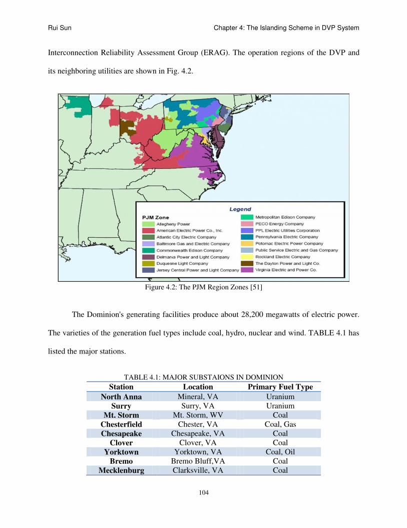
Rui Sun Chapter 4: The Islanding Scheme in DVP System
104
Interconnection Reliability Assessment Group (ERAG). The operation regions of the DVP and
its neighboring utilities are shown in Fig. 4.2.
Figure 4.2: The PJM Region Zones [51]
The Dominion's generating facilities produce about 28,200 megawatts of electric power.
The varieties of the generation fuel types include coal, hydro, nuclear and wind. TABLE 4.1 has
listed the major stations.
TABLE 4.1: MAJOR SUBSTAIONS IN DOMINION
Station Location Primary Fuel Type
North Anna Mineral, VA Uranium
Surry Surry, VA Uranium
Mt. Storm Mt. Storm, WV Coal
Chesterfield Chester, VA Coal, Gas
Chesapeake Chesapeake, VA Coal
Clover Clover, VA Coal
Yorktown Yorktown, VA Coal, Oil
Bremo Bremo Bluff,VA Coal
Mecklenburg Clarksville, VA Coal

Rui Sun Chapter 4: The Islanding Scheme in DVP System
105
North Branch Bayard, WV Coal
Altavista Altavista, VA Coal
Southampton Southampton, VA Coal
Hopewell Hopewell, VA Coal
Possum Point Dumfries, VA Gas, Oil
Elizabeth River Chesapeake, VA Gas
Ladysmith Ladysmith, VA Gas
Bellemeade Richmond, VA Gas
Rosemary Roanoke Rapids, NC Gas
Darbytown Richmond, VA Gas
Bath County Warm Springs, VA Water
Gaston Roanoke Rapids, NC Water
Roanoke Rapids Roanoke Rapids, NC Water
Gordonsville Gordonsville, VA Gas
The Virginia Power system is geographically dispersed with major generation and load
centers. And according to [17], there are some heavily loaded areas in the DVP system. They
may become the major weak points during potential islanding conditions because these areas
may face serious generation-load unbalanced situations. Besides, the Virginia Power system is
located on the east coast of the United States, where is affected by windstorm and thunder storms.
These severe weather conditions are major causes in tripping of heavily loaded transmission
lines. One example of this vulnerability was Hurricane Irene which made its landfall over
Eastern North Carolina's Outer Banks on the morning of August 27, 2011. This powerful
Atlantic hurricane caused one of the major 500kV transmission lines in DVP to trip. Under
certain circumstances, the heavy load situation and severe weather conditions may interact and
result in additional cascading trips, forming island within the DVP areas. The decision of
potential islanding areas is based on a consideration of these aspects.
In history, the DVP system was often influenced by bad weather situations: lightning,
heavy winds, hurricanes, ice and snow. However no islanding situation has been experienced in
the DVP. The closest case was a severe disturbance happened close to the Yorktown station.

Rui Sun Chapter 4: The Islanding Scheme in DVP System
106
Though no islanding has occurred, there is always a possibility and online fast-prediction to such
catastrophic scenarios is essentially necessary.

Rui Sun Chapter 4: The Islanding Scheme in DVP System
107
4.2 Online Islanding Detection Module Schemes
4.2.1 Methodology
Figure 4.3 has illustrated the structure of the PMU application in Dominion including the
islanding detection and protection strategy.
Figure 4.3: Structure of the Dominion Online System Monitoring and Protection Software
Real time PMU measurements are collected and transmitted back to the local server by an
openPDC data concentrator. The raw data go through the processing stage in system topology
configuration module, the calibration module and the state estimator module. The processed data
are then used for islanding detection and state evaluation. The analyzed results are saved in
historian module.
The proposed islanding detection methodology is part of the system monitoring and
protection implementation. An investigation of possible islanding contingency cases in
Dominion territory is carried out and the decision trees for islanding detection and identification
are generated. However several aspects are modified subject to the practical condition in the

Rui Sun Chapter 4: The Islanding Scheme in DVP System
108
DVP system: 1) the determination of the potential islanding areas was primarily based on
discussion and analysis of the geographical/electrical characteristics and historical cascading
disturbance events in the DVP. According to the VT Power group and the Dominion group,
three major areas were selected. 2) The PMU installation list and schedule for the DVP is well
established and the islanding analysis focuses on this list. By the end of 2014, there will be 20
substations in the DVP system having PMUs implemented and the whole 500kV transmission
network and portion of the 230/115kV network will be observable in real time. This study is
primarily focused on the observed network to study the potential islanding events in the low
voltage area.
Fig. 4.4 illustrates the decision tree based islanding detection and identification scheme
that includes the following procedures:
1) The determination of the potential islanding locations; the DT analysis are carried out
at three different regions in the DVP system. The three regions are named as Region-1: Newton
station area, Region-2: Einstein and Dirac station area and Region-3: Franklin and Raphson
station area.

Rui Sun Chapter 4: The Islanding Scheme in DVP System
109
Figure 4.4: The DT Based Islanding Scheme Procedures
2) In each region, the system one line diagram and cut-off locations are created based on
the geographical/electrical distribution. The detailed geographical map and islanding cut-off
sections of location one can be seen in Fig. 3.6 and Fig. 3.7.
The decision of the island size is first performed based on the geographic map of Fig. 3.6.
The isolated area analysis starts from the selected sub-station and radiates outwards. For each of
the two directions, the transmission lines come out of the station circles with increasing radius
which indicates a growth of the possible islanding area along the transmission paths. In the
corresponding system one-line diagram shown in Fig. 3.7, the whole area is separated into four
partitions (0-3) for a convenient load calculation. The partitioning determination is based on the
system topology characteristics and load condition. The potential islanding regions are labeled
by the cut-off locations using dotted lines.

Rui Sun Chapter 4: The Islanding Scheme in DVP System
110
3) Dynamic simulations are carried out for the three locations. When applying the
simulation, the under-frequency load shedding scheme for DVP is considered. The scheme
allows a maximum shedding of 30% of the total load during the protection operation. The time
for communication delay and relay/breaker operation for each shedding is set to be 0.2833 sec.
On the other hand, when the generation exceeds the load in an island, the intelligent generator
shedding will apply, the excessive generation will be tripped if area frequency exceeds 61.8Hz
for ten seconds or immediately when the frequency reaches 64.8Hz. Any island that fails to keep
the area frequency beyond 58.5Hz after performing the load/generation shedding scheme is
considered unstable.
4) To achieve the module’s function, four decision tree sets are generated using different
data sets. DT-1 is used to achieve a full area islanding detection and identification. It is also
responsible for the location estimate, delivering input measurements to the correct sub-system
DT for further operation. DT-2 to DT-4 are three sub-system DTs for the three locations that
estimate: 1) the islanding stability condition, 2) the approximate islanded region size (isolated
generation capacity). Because each tree set achieves two functions and each function requires a
specific tree there are eight individual decision trees, while the trees in the same set share one
common attribute dataset. Fig. 4.5 has illustrated the detailed online islanding module functions.
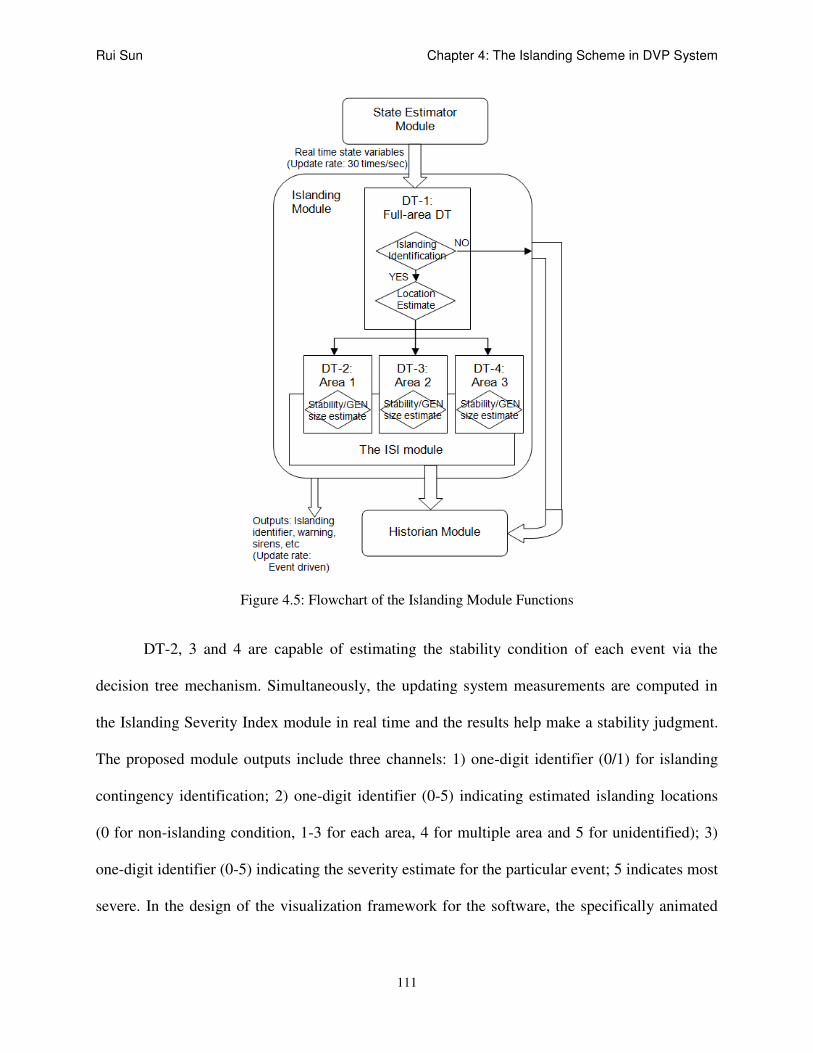
Rui Sun Chapter 4: The Islanding Scheme in DVP System
111
Figure 4.5: Flowchart of the Islanding Module Functions
DT-2, 3 and 4 are capable of estimating the stability condition of each event via the
decision tree mechanism. Simultaneously, the updating system measurements are computed in
the Islanding Severity Index module in real time and the results help make a stability judgment.
The proposed module outputs include three channels: 1) one-digit identifier (0/1) for islanding
contingency identification; 2) one-digit identifier (0-5) indicating estimated islanding locations
(0 for non-islanding condition, 1-3 for each area, 4 for multiple area and 5 for unidentified); 3)
one-digit identifier (0-5) indicating the severity estimate for the particular event; 5 indicates most
severe. In the design of the visualization framework for the software, the specifically animated

Rui Sun Chapter 4: The Islanding Scheme in DVP System
112
flashing area signals and sirens are considered for the islanding warning purpose in the DVP full-
loop geographical system diagram screen.
It is suggested to rerun the offline DT program, generating the updated DTs from
modified database in the aid of the historian module. A suggested refreshing rate is no longer
than once a month with minute contingencies and immediate after severe system
disturbances/contingencies or significant structure changes.

Rui Sun Chapter 4: The Islanding Scheme in DVP System
113
4.3 Study of the Islanding Scenarios in DVP System
To initialize the database, a total of 678 islanding events were simulated and analyzed
(130 cases for Area-1, 396 for Area-2 and 152 for Area-3, basing on their complexity). Together
with 501 non-islanding cases (301 normal operation cases; 100 short circuit and rapid load
changing fault cases and 100 line tripping cases), the size of the islanding database is 1179*87.
(87 is the channel number of the simulation outputs). The attribute categories are voltage
magnitudes, voltage angles and current phasors.
With the original islanding case database, it is possible to compute the prediction success
for the original DTs. The specifics and prediction success are list in TABLE 4.2 and 4.3.
TABLE 4.2: DT SPECIFICS
DT name DT1:
Full DVP
DT2:
Area 1
DT3:
Area 2
DT4:
Area 3
Total case # 1179 631 897 753
Islanding
case# 678 130 396 152
Stable cases - 126 271 84
Channel # 87 87 87 87
TABLE 4.3: DT PREDICTION SUCCESS
DT name
The DTs in Dominion
DT1:
Full DVP
DT2:
Area1
DT3:
Area 2
DT4:
Area 3
Islanding
detection
Size 9
NA NA NA
Learn 97.20
Test 95.67
Location
estimate
Size 13
Learn 99.07
Test 97.71
Stability
estimate
Size
NA
2 12 11
Learn 100 93.43 89.92
Test 100 90.40 80.92
GEN size
estimate
Size 2 12 3
Learn 100 80.56 100
Test 100 74.24 98.68

Rui Sun Chapter 4: The Islanding Scheme in DVP System
114
In general, the full loop DTs achieves over 95% average success for both islanding
identification and location estimate with the original data. The DT-2 achieves a high stability and
GEN size estimate due to the simplicity of the area while the DT-3 performs high accuracy in
stability estimate but 74% accuracy in GEN size estimate. The DT-4 has a moderate 81%
stability estimate success and works well in GEN size estimate.
4.3.1 Decision Tree Analysis
A comparison has been taken among decision trees on their tree structure, composition,
and diversity in this section, corresponding analysis is applied.
4.3.1.1 Decision Tree Size Analysis
The first comparison is about the tree size. DT-2 is simple in its structure and is excluded
from the comparison. Fig. 4.6 indicates that all DT sets are rather similar in size. Tree-1 and
Tree-2 refer to trees with different functionalities in one tree set. For DT-1, they are islanding
detection and location estimate; for DT-2 to DT-4, they are stability estimate and power capacity
estimate. To achieve a prediction success between 80%-100%, a tree needs to grow to around 12
nodes. This is not a bad score for decision trees. However, the simplicity (or complexity) of the
tree is largely dependent on the corresponding complexity of the attribute dataset and the tree
functionality. In the Dominion case, the tree size largely depends on the geographical complexity
of the area and the power system diversity (i.e. the number of the plants and generators, the
length and number of the transmission lines, the tie-line number of the area and the capacitor
banks number, etc). Among the three locations, the area-2 has the largest power capacity and
plant number, as well as the tie-line number. This is reflected in the total number for the two
functional trees. The whole area tree is also respectively large in size due to the size of its dataset.

Rui Sun Chapter 4: The Islanding Scheme in DVP System
115
However the functions of DT-1 are different from the other trees thus the size of DT-1 is not far
beyond sub-system trees.
Figure 4.6: Decision Tree Size Comparison (after Prune)
In addition, the trees are manually pruned in order to achieve a balance between size and
precision. Fig. 4.7 shows the original tree size comparison. It’s easy to notice the Tree-2 in DT-3
and Tree-1 in DT-4 have the largest size. This indicates that CART may have difficulty
generating highly converged trees using the present datasets. This is proofed by their low
prediction success: 85%/75% un-pruned and 80%/74% pruned for Tree-2 in DT3, and 90.5%/82%
un-pruned and 90%/82% pruned for Tree-1 in DT4. An 80% precision is still valuable for system
state estimation and evaluation and could be used to implement the islanding judgment. If the
system requires higher precision, two strategies can be used to modify the tree: 1) importing
more cases into the dataset; 2) increase the attribute quantity. In decision tree principle, both
strategies are designed to include more information about the system thus decrease the use of the
twisted relationships among present attributes.
0
2
4
6
8
10
12
14
DT-1
DT-3
DT-4
9
12
11
13
12
3
Tree-1
Tree-2

Rui Sun Chapter 4: The Islanding Scheme in DVP System
116
Figure 4.7: Decision Tree Size Comparison (before Prune)
4.3.1.2 Attributes Analysis
The second comparison relates the major splitting attribute types, still using the six
decision trees in previous comparison. In this comparison, two calculations are performed: the
major splitting attributes in formed tree and the important variables for all (including splitting
points, surrogates and pruning).
Figure 4.8: Decision Tree Attribute Type Comparison (Tree only)
0
5
10
15
20
25
DT-1
DT-3
DT-4
9 12 14
13
21
3
Tree-1
Tree-2
0
2
4
6
8
DT-1,
Tree1DT-1,
Tree2DT-3,
Tree1DT-3,
Tree2DT-4,
Tree1DT-4,
Tree2
5
2 2
1
4
3
0 0
0 0
0 0
2
6 7
6
5
1
Voltage Mag
Voltage Ang
Current Phasor

Rui Sun Chapter 4: The Islanding Scheme in DVP System
117
The current phasor measurements exported from simulation software are complex values
X+jY. Instead of using complex values, the current phasors are converted into single values using
Fisher’s method applied to phasor measurements [52] (will be discussed in Section 4.6). An
analysis of the benefits using this transformation or polar form current phasors will be given in
Section 4.6. The major attributes used to form the trees are voltage magnitude and current phase.
By decision tree functions, the voltage magnitudes are used more than current phases in
islanding detection while the current phases are most important judgments for islanding location
estimate, stability estimate and power capacity estimate. The reason why voltage angles become
less important is that the recorded inputs are at the 500kV network and they remain connected
with the massive power system and keep stable after the initial oscillation when islanding occurs.
Compared with angles, the current phasor and voltage magnitude changes are much more
apparent, especially for buses near the boundaries of the isolation. CART automatically selects
attributes with larger influences to build the tree, and to some extent, it has proven that the
current phasor and voltage magnitudes are more important variables for islanding analytics.
Figure 4.9: Decision Tree Attribute Type Comparison (for all)
0
2
4
6
8
10
12
14
16
18
20
DT-1,
Tree1DT-1,
Tree2DT-3,
Tree1DT-3,
Tree2DT-4,
Tree1DT-4,
Tree2
13
10
14
8
16
9
0
8 9
7
6
3 0
19 19
15
11
4
Voltage Mag
Voltage Ang
Current Phasor

Rui Sun Chapter 4: The Islanding Scheme in DVP System
118
Taking into consideration the important variables for all (including splitting points,
surrogates and pruning), more attributes are involved in the tree formation. Shown in Fig. 4.9,
the number of each attribute category is calculated. In such case, there are also voltage angle
attributes that are selected as surrogates or back-up splitting points in the tree formation.
4.3.2 Islanding Variable Importance Analytics
With the benefit of decision trees, the appearance and importance of each Dominion’s
500kV substation in the DT formation was calculated and analyzed. Shown in TABLE 4.4:
TABLE 4.4: SUBSTATION APPEARANCE IN DT FORMATION
Substation# DT1-1 DT1-2 DT2-1 DT2-2 DT3-1 DT3-2 Rank
314900 1 1 1 1 1 A
314901 1
314902 1 1 1 1 1 A
314903 1 1 1 C
314904 1 1 1 C
314905
314906 1
314907 1 1
314908 1 1 1 1 B
314909
314910 1
314911 1 1 1 C
314912
314913
314914 1 1 1 C
314915 1
314916 1 1
314917 1
314918 1 1
314919 1
314922 1
314923 1
314924 1 1 1 C
314925 1
314926 1
314927 1 1 1 1 B
314928 1 1 1 1 1 1 A

Rui Sun Chapter 4: The Islanding Scheme in DVP System
119
Among the 29 500kV substations and six decision trees, measurements from 3 locations
are used by five DTs, 2 substations used four times and 5 substations used three times. The ten
locations (314900, 314902, 314928, 314908, 314927, 314903, 314904, 314911, 314914 and
314924) are considered to be critical locations for Dominion Islanding detection.
Another calculation is carried out using the variable importance computation function
from CART. For each variable in each tree, the software computes the relative importance of the
variable and normalizes its value to the maximum variable.
TABLE 4.5: SUBSTATION IMPORTANCE IN DT FORMATION
Substation# DT1-1 DT1-2 DT2-1 DT2-2 DT3-1 DT3-2 Total Rank
314900 2.36 113.83 40.23 23.86 180.28 C
314901 56.24 45.76 102 C
314902 60.06 26.31 36.43 122.23 245.03 B
314903 5.36 7.49 10.93 23.78
314904 9.6 1.33 83.02 93.95
314905 0
314906 16.63 16.63
314907 2.02 73.46 75.48
314908 5.36 66.48 73.21 100 245.05 B
314909 0
314910 2.02 2.02
314911 58.99 62.28 122.22 243.49 B
314912 0
314913 0
314914 26.31 65.79 40.56 132.66 C
314915 43.97 100 143.97 C
314916 100 40.23 140.23 C
314917 40.98 40.98
314918 65.79 42.98 108.77 C
314919 23.86 23.86
314922 0
314923 42.53 100 142.53 C
314924 78.36 142.53 220.89 B
314925 12.97 12.97
314926 40.98 40.98
314927 104.22 89.94 91.54 285.7 B
314928 7.65 89.94 100 78.36 256.62 532.57 A

Rui Sun Chapter 4: The Islanding Scheme in DVP System
120
The substation importance to each tree and the total module is shown in TABLE 4.5.
Based on the total value, ranks are also assign ranks to them and there are six locations reaching
a value over 200%. They are 314928, 314927, 314908, 314902, 314911 and 314924. From
another point of view, this calculation illustrates the order of importance for present substations
in Dominion’s islanding detection. This calculation counts every splitting point in the tree that if
any location appears repeatedly the variable importance will also be computed repeatedly.
Both tests have demonstrated some common facts about the DT’s variable importance in
Dominion’s islanding module.
1) Geographically, the measurements from the substations closer to the islanded area
may contribute more in islanding detection and classification. Generally, during the faults, the
nearby monitors are capable of collecting signals with more information and details about the
voltage/current/frequency oscillation and drops than those monitor at far end. Substation 314928,
314902, 314924, and 314927 are located in places surrounded by three potential islanding
regions thus they are ranked highest in DT formation.
2) Substations with tie-lines having high current transmissions may contribute more in
islanding detection and classification. The sudden power drop of the isolated area causes great
impact to the main power grid and those transmission lines carrying high power will mostly
influenced.

Rui Sun Chapter 4: The Islanding Scheme in DVP System
121
4.4 Islanding Analysis with the Consideration of internal PMUs
In the future plans of the Dominion’s PMU installation project, a few of 230/115kV
substations/grids will have PMU installed. For islanding consideration, this indicates that a wider
variety of measurements and locations can be used in the decision tree algorithms. In this section,
a selected set of islanding contingency simulations with additional 230/115kV measurement
outputs are run and analyzed. The modified simulations cover all three locations in the previous
analysis. It should be noticed that in this section all current phasors are used in polar form.
4.4.1 DT Improvement Test: Region-1
In this test, a few internal PMUs are added at critical locations (plants, large loads, major
power-flow injection buses…etc.) at lower voltage level (115KV/230KV) in Region-1. The
additional PMUs measure the local bus’ voltage phasors, current phasors and frequencies.
TABLE 4.6: INTERNAL PMUS IN REGION-1
Selected PMU location
(Bus number)
Voltage
level Area # Priority
Generator bus 314422 115KV
1 1 314423 230KV
Large load 314373 115KV 1 3
Large load 314413 230KV 1 3
Large load 314421 230KV 1 3
Large load 314398 230KV 1 3
Large load 314406 115KV 1 3
Transformer
bank
314401 115KV 1 3
314402 230KV
Transformer
bank
314406 115KV 1 3
314407 230KV
Transformer
bank
314417 115KV 1 3
314418 230KV
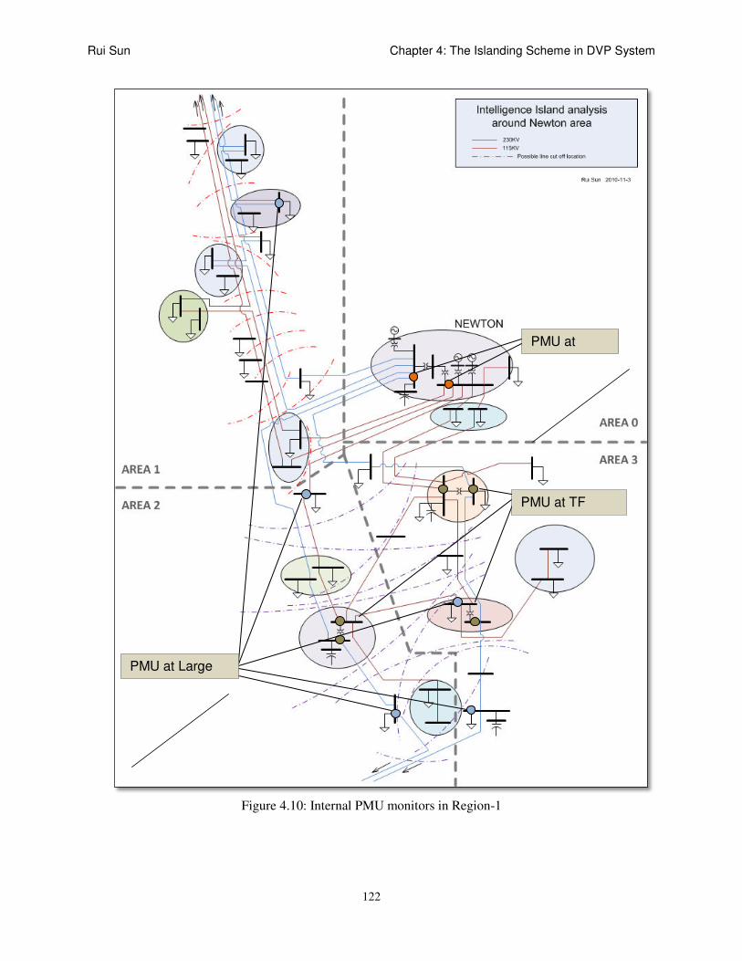
Rui Sun Chapter 4: The Islanding Scheme in DVP System
122
Figure 4.10: Internal PMU monitors in Region-1
PMU at TF
PMU at Large
PMU at

Rui Sun Chapter 4: The Islanding Scheme in DVP System
123
A total of 9 internal locations are selected in this test due to their importance. The same
islanding simulations are run and decision trees for islanding detection for Region-1 are
generated using the enlarged dataset. The DT relative cost comparison is shown in Fig. 4.11.
Figure 4.11: DT relative cost comparison in Region-1
With the modified dataset, the prediction success of islanding detection for Region-1 are
99.21%/98.73% for learn/test group with only 500kV measurements and 99.84%/99.68% with
internal PMUs. At the same time, the tree sizes are both 3 nodes for optimal placement. This
indicates both trees have high precision in islanding detection.
Another comparison is taken place on the variable importance. We can notice the internal
channels are selected as variable importance when they contain more useful information.
TABLE 4.7: VARIABLE IMPORTANCE COMPARISON – REGION-1
1 1.5 2 2.5 3 3.5 4 4.5 50
0.005
0.01
0.015
0.02
0.025
0.03
0.035
0.04
0.045
Number of nodes
Rela
tive C
ost
DT: 500kV
DT: with internal data
DT with only 500kV data DT with lower voltage data
Variables Score Variables Score I_MAG_314923_314924 100.00 A314407 100.00
A314923 96.84 A314406 100.00
I_ANG_314915_314923 92.29 I_MAG_314923_314924 96.85
I_ANG_314902_314906 91.77 A314923 93.79
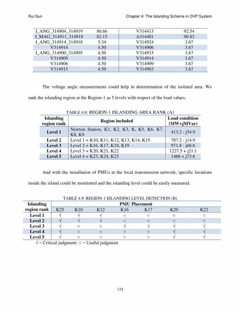
Rui Sun Chapter 4: The Islanding Scheme in DVP System
124
The voltage angle measurements could help in determination of the isolated area. We
rank the islanding region at the Region-1 as 5 levels with respect of the load values.
TABLE 4.8: REGION-1 ISLANDING AREA RANK (A)
Islanding
region rank Region included
Load condition
(MW+jMVar)
Level 1 Newton Station, K1, K2, K3, K, K5, K6, K7,
K8, K9 413.2 - j54.9
Level 2 Level 1 + K10, K11, K12, K13, K14, K15 787.2 - j14.9
Level 3 Level 2 + K16, K17, K18, K19 971.8 - j66.6
Level 4 Level 3 + K20, K21, K22 1227.5 + j21.1
Level 5 Level 4 + K23, K24, K25 1466 + j73.6
And with the installation of PMUs at the local transmission network, specific locations
inside the island could be monitored and the islanding level could be easily measured.
TABLE 4.9: REGION-1 ISLANDING LEVEL DETECTION (B)
Islanding
region rank
PMU Placement
K25 K10 K12 K16 K17 K20 K22
Level 1 √ √ √ ○ ○ ○ ○
Level 2 √ √ √ ○ ○ ○ ○
Level 3 √ ○ ○ √ √ √ √
Level 4 √ ○ ○ ○ ○ √ √
Level 5 √ ○ ○ ○ ○ √ √
√ = Critical judgment; ○ = Useful judgment.
I_ANG_314904_314919 86.66 V314413 92.54
I_MAG_314911_314918 82.15 A314401 90.83
I_ANG_314914_314918 5.34 V314924 3.67
V314914 4.50 V314906 3.67
I_ANG_314900_314905 4.50 V314915 3.67
V314909 4.50 V314914 3.67
V314906 4.50 V314909 3.67
V314915 4.50 V314903 3.67

Rui Sun Chapter 4: The Islanding Scheme in DVP System
125
4.4.2 DT Improvement Test: Region-2
For Region-2, the major comparison is made upon the GEN size estimate, which is not
very well determined by the original tree. In this test, 10 locations at lower voltage level
(115KV/230KV) in Region-2 have PMU monitors implemented. The original dataset fails to
offer adequate information for the DT so that the DT prediction success falls to 80%. With the
internal system measurements, the new tree achieves a prediction success to 100%. It’s a great
leap in estimate success and the new tree only requires 5 nodes to complete the prediction.
TABLE 4.10: REGION-2 ISLANDING GEN SIZE ESTIMATE COMPARISON
Figure 4.12: DT relative cost comparison in Region-2
0 5 10 15 20 25
0
0.2
0.4
0.6
0.8
1
Number of nodes
Rela
tive C
ost
DT with 500KV Data
DT with internal Data
DT with only 500kV data DT with lower voltage data
Learn Test Learn Test
% Overall
correct 86.62 74.24 100 100

Rui Sun Chapter 4: The Islanding Scheme in DVP System
126
The test results indicate that the local PMU measurements could offer important
information of system operation behaviors during islanding scenarios. According to the analysis
of system variable importance for both trees, we notice the local voltage magnitudes and angles,
along with the frequency parameters are essential measurements in GEN size estimation.
TABLE 4.11: VARIABLE IMPORTANCE COMPARISON – REGION-2
4.4.3 DT Improvement Test: Region-3
In this test, 11 locations at lower voltage level (115KV/230KV) in Region-3 have PMU
monitors implemented and the DT analysis is carried out. The original DT reached 99.8%
precision in islanding detection, so the most apparent improvement comes from the stability
DT with only 500kV data DT with lower voltage data
Variables Score Variables Score
A314906 100.00 A314275 100.00
I_ANG_314924_314928 66.43 F314275 95.88
V314908 32.85 V314275 55.40
I_MAG_314908_314911 32.53 A314906 38.53
I_MAG_314909_314923 27.28 V314254 33.33
V314900 22.77 A314254 33.33
I_ANG_314902_314928 20.84 A314274 33.33
V314916 20.11 V314276 33.33
V314919 19.83 A314289 33.33
I_ANG_314914_314918 16.38 V314289 30.76
A314909 15.34 I_ANG_314924_314928 22.19
I_ANG_314923_314924 12.91 I_MAG_314909_314923 19.15
A314927 12.02 F314289 18.18
A314903 11.99 V314236 16.98
I_ANG_314911_314918 11.18 I_MAG_314919_314922 14.49
V314914 11.16
V314902 10.57
A314914 10.54
I_MAG_314900_314916 10.23
I_ANG_314915_314923 9.70

Rui Sun Chapter 4: The Islanding Scheme in DVP System
127
estimate. According to Fig. 4.13 and TABLE 4.12, with the enlarged dataset, the tree size largely
decreased (from 12 nodes to 3 nodes) while the precision raises over 10% (from 80-90% to 98%).
TABLE 4.12: REGION-3 ISLANDING STABILITY ESTIMATE COMPARISON
Figure 4.13: DT stability estimate comparison in Region-3
The improvement largely results from the usage of the internal frequency (phasor angle)
measurements. The major variables used to form the new tree are frequency measurements for
the great oscillation and phase shifts during the transients. By analysis it was proved that the
internal PMUs could offer essential information for the islanding detection and qualification,
especially for island stability estimation and size estimation. Yet there are other concerns that
need to be solved:
1) Can the local PMU measurements help to judge the entire system’s islanding situation?
(i.e. an islanding occurs in other area)
2 4 6 8 10 120
0.1
0.2
0.3
0.4
0.5
0.6
0.7
0.8
0.9
Number of modes
Rela
tive C
ost
DT with 500kV Data
DT with Internal Data
DT with only 500kV data DT with lower voltage data
Learn Test Learn Test
% Overall
correct 94.08 78.95 100 98.03

Rui Sun Chapter 4: The Islanding Scheme in DVP System
128
2) What are the most proper locations for local PMU implementation with consideration
of the entire system? (Introducing the local measurements to the whole system DT)
To solve these questions, a further investigation and analysis is needed thorough the re-
simulation of the whole system.

Rui Sun Chapter 4: The Islanding Scheme in DVP System
129
4.5 Islanding Analysis with the Light Load Model
In this section, how the differences of the system operational conditions will contribute to
the programmatic model simulation, analytics and decision tree formation in Dominion is
analyzed.
In Chapter 3, the model used for DVP simulation and decision tree scheme was
introduced. The major study system used is a modified MMWG 57,000 Bus Eastern Coast Power
Grids model. In this model, the Dominion Transmission System operates on the edge of its
power capacity. While in real world, the power generation and consumption are always dynamic.
One power system has its summer and winter load peaks and tends to follow certain annual
operation cycles. On the other hand, its everyday operation behavior also follows certain curve.
Fig. 4.14 shows the annual load demand peaks for the DVP from 1997 to 2011.
Figure 4.14: Annual Peak Load Demand for DVP [53]

Rui Sun Chapter 4: The Islanding Scheme in DVP System
130
The maximum load demand mostly occurs in summer whose power consumption is the
highest during a one year period. The power demand in winter is relatively mild and is very
different from the summer. Similarly, the daily load demand follows another curve, respectively.
Normally, this dynamic behavior is not simulated by the power flow analysis since the
system load model is fixed. Thus it may be inadequate if only the fixed load model is used for
the system analysis for the lack of describing system’s dynamic operating conditions. In this
section, the decision tree scheme in system islanding detection is studied using different load
models. As introduced earlier, the model works under Dominion’s “Summer Heavy load”
condition. Based on the present model, a modified “summer light-load” model is created
applying percentage load decrements. Certain capacitor banks, transformer taps and model
dynamic parameters are tuned in order to maintain the bus voltage and angles. The light-load
model operates approximately at 65% of the heavy load model.
The simulation is carried out on Region-1. The same 130 islanding contingency cases
with 500 non-islanding cases are repeated in the same way as in Section 4.4.1. Two data sets are
used for decision tree generation. They are the:
1) Voltage and current phasors at all external PMU locations.
2) Voltage and current phasors at all external PMU locations and voltage, current and
frequency channels at internal (potential) PMU locations.
The current attributes are in polar form.
The new DTs have distinct differences from the heavy-load model DTs, yet they still
share some common characteristics. For this analysis, a comparison is made among the new DTs
and DTs used for Section 4.41. A total of four decision trees are compared.
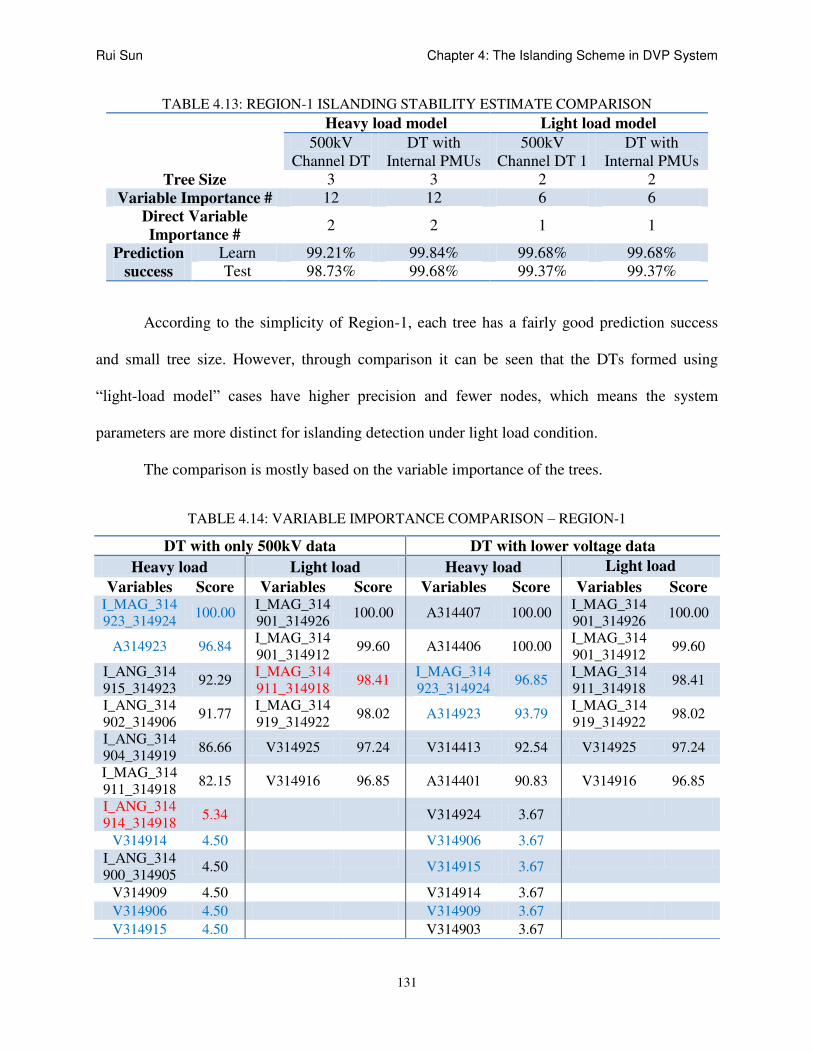
Rui Sun Chapter 4: The Islanding Scheme in DVP System
131
TABLE 4.13: REGION-1 ISLANDING STABILITY ESTIMATE COMPARISON
Heavy load model Light load model
500kV
Channel DT
DT with
Internal PMUs
500kV
Channel DT 1
DT with
Internal PMUs
Tree Size 3 3 2 2
Variable Importance # 12 12 6 6
Direct Variable
Importance # 2 2 1 1
Prediction
success
Learn 99.21% 99.84% 99.68% 99.68%
Test 98.73% 99.68% 99.37% 99.37%
According to the simplicity of Region-1, each tree has a fairly good prediction success
and small tree size. However, through comparison it can be seen that the DTs formed using
“light-load model” cases have higher precision and fewer nodes, which means the system
parameters are more distinct for islanding detection under light load condition.
The comparison is mostly based on the variable importance of the trees.
TABLE 4.14: VARIABLE IMPORTANCE COMPARISON – REGION-1
DT with only 500kV data DT with lower voltage data
Heavy load Light load Heavy load Light load
Variables Score Variables Score Variables Score Variables Score I_MAG_314
923_314924 100.00
I_MAG_314
901_314926 100.00 A314407 100.00
I_MAG_314
901_314926 100.00
A314923 96.84 I_MAG_314
901_314912 99.60 A314406 100.00
I_MAG_314
901_314912 99.60
I_ANG_314
915_314923 92.29
I_MAG_314
911_314918 98.41
I_MAG_314
923_314924 96.85
I_MAG_314
911_314918 98.41
I_ANG_314
902_314906 91.77
I_MAG_314
919_314922 98.02 A314923 93.79
I_MAG_314
919_314922 98.02
I_ANG_314
904_314919 86.66 V314925 97.24 V314413 92.54 V314925 97.24
I_MAG_314
911_314918 82.15 V314916 96.85 A314401 90.83 V314916 96.85
I_ANG_314
914_314918 5.34
V314924 3.67
V314914 4.50 V314906 3.67 I_ANG_314
900_314905 4.50
V314915 3.67
V314909 4.50 V314914 3.67 V314906 4.50 V314909 3.67 V314915 4.50 V314903 3.67
Rui Sun Chapter 4: The Islanding Scheme in DVP System
132
TABLE 4.14 lists the variable importance for each decision tree formation. The two DTs
for light-load condition are the same; they have the same tree structure and variables. The two
DTs for heavy-load condition share several common attributes in tree formation. However, there
is only a slight relation between DTs of two models. Thus the two sets of DTs are almost
irrelevant.
The test results raise one important issue: will the lack of the dynamic system operational
behaviors cause the DT algorithm to miss certain important system measurements in islanding
detection? The answer is yes. However this issue can be greatly compensated by many aspects:
First, on the analytics side, although it is impossible to consider all system operating
conditions in the simulation stage, the tests can be applied on several typical operating condition
models, i.e. the summer heavy-load, summer light-load, winter heavy-load, winter light-load,
and etc. Different models of different seasons indicate not only load demand changes, but also
different line & generation operating schemes, protection schemes and power injection
conditions. The more detailed models are used in decision tree database, the wider the range of
conditions and information that can be implemented into the islanding scheme.
Second, for the utilities’ practical usage, the islanding module is designed to be capable
of selecting the most proper DTs depending on its operating scheme, while all DTs are pre-
generated during the offline procedure using different models. The islanding module
modification is also dynamic. As discussed in Section 4.2.1, the tree is suggested to be updated
every month to follow certain changes on system topology and projected maintenances. While in
operation, the historian module brings in database the real-world data, increasing the data’s
accuracy and the trees’ credibility.

Rui Sun Chapter 4: The Islanding Scheme in DVP System
133
Last but not least, the heavy-load model is more suitable for islanding analysis than the
light-load model. Taking into consideration the power system strain level, a system is easier to
collapse under heavy-load condition than working in the light-load mode while facing the same
amount of stress. Many islanding cases (i.e. the 1973 Gulf coast area islanding) have
demonstrated that the disturbances occurred while the transmission networks were under the
peak-load demands, which weakened the systems stability margin. Besides load condition, the
climate condition is another consideration. Summer and winter are two hostile seasons that are
easier for islanding contingencies to occur (see TABLE 4.15).
TABLE 4.15: NERC ISLANDING CASES OCCURANCE
Total case analyzed: 19
Season Summer (6,7,8,9) 9
Winter (11,12,1) 7
Hour Peak hour (10-23) 10
Off peak hour 7

Rui Sun Chapter 4: The Islanding Scheme in DVP System
134
4.6 Analysis of Fisher’s method applied to Islanding DT Attributes
In Section 4.3, decision trees are generated and analyzed for islanding detection and
identification, stability estimate and island size estimate. In Section 4.4 and 4.5, DTs using low
voltage network parameters and light load model are introduced. There’s a difference between
them, the current attributes of the former case DTs are in single value form converted by the
Fisher’s method, while for the latter DTs they are in polar form. In this section, the principle and
usage of the Fisher’s method applied to phasor measurements in DT algorithm is discussed. The
test results using the Fisher’s method and polar form for attributes are compared and analyzed.
CART uses a non-parametric decision tree learning technique that is especially suited to
power systems due to the complex non-linear behavior of the system. CART data is in the form
of an array with rows being the events/outcomes and columns being the measurements. In its
simplest form, CART picks one measurement at a time for performing binary splits. While this is
very effective in handling data having invariate attributes, difficulties are observed when
handling multi-modal classifications consisting of multivariate data. Traditionally, CART makes
decisions based on a single attribute. However, because phasor data has two components, both
must be considered simultaneously to make correct decisions. Furthermore, it has been
determined that there is a need to make multi-class distinctions instead of only binary splits.
Therefore, a methodology was developed that extended the use of Fisher’s Linear Discriminant
(FLD) to perform splits on high dimensional, multi-class data [52, 54]. In principle, while using
the Fisher’s method applied to the phasor measurements new attributes are formed through a
linear transformation of one or multiple related phasor attribute pairs (which are directly
obtained from simulations or real measuring process). The new attributes contain the
characteristics of multiple existing phasor attributes and when used to form the decision trees by

Rui Sun Chapter 4: The Islanding Scheme in DVP System
135
replacing the existing phasor attribute pairs, they keep the tree from making decision only on
single attribute from the pairs and to some extent raise the prediction success of the DTs.
In islanding analysis, along with the normal polar form current measurements, the
Fisher’s method is analyzed and the results are compared with the original data. TABLE 4.16
shows the comparison in both the tree prediction success and variable importance. The analysis
used both Region-2 and Region-3.
TABLE 4.16: DT PREDICTION SUCCESS COMPARISON – PREDICTION SUCCESS
DT name
DT-3: Region-2 DT-4: Region-3
Fisher’s
method
Polar form
phasor
Fisher’s
method
Polar form
phasor
Stability
estimate
Size 12 9 11 12
Learn 93.43 93.43 90.13 94.08
Test 90.40 87.88 82.24 78.95
GEN size
estimate
Size 24 21 3 3
Learn 85.35 86.62 100 100
Test 75.51 74.24 98.68 98.68
TABLE 4.17: DT VARIABLE IMPORTANCE COMPARISON – GENSIZE
DT-3: Region-2 DT-4: Region-3
Fisher’s method Polar form phasor Fisher’s method Polar form phasor
I_314908_314911 A314906 I_314915_314923 A314927
I_314900_314905 I_ANG_314924_31492
8
I_314902_314915 A314928
I_314924_314928 V314908 V314901 I_MAG_314924_314928
V314908 I_MAG_314908_31491
1
V314922 I_MAG_314915_314923
I_314905_314911 I_MAG_314909_31492
3
V314907 I_MAG_314902_314915
I_314902_314906 V314900 V314912 A314909
I_314904_314919 I_ANG_314902_31492
8
V314926 I_ANG_314911_314922
I_314902_314914 V314916 A314902 I_ANG_314908_314911
I_314911_314918 V314919 A314903 A314906
V314903 I_ANG_314914_31491
8
V314903 I_ANG_314917_314926
I_314919_314922 A314909 V314904 A314902
I_314914_314918 I_ANG_314923_31492
4 I_ANG_314919_314922
A314902 A314927
A314927 A314903

Rui Sun Chapter 4: The Islanding Scheme in DVP System
136
A314909 I_ANG_314911_31491
8 A314923 V314914
A314915 V314902
I_314915_314923 A314914
I_314902_314915 I_MAG_314900_31491
6 V314925 I_ANG_314915_31492
3
TABLE 4.18: VARIABLE IMPORTANCE COMPARISON – STABILITY
DT-3: Region-2 DT-4: Region-3
Fisher’s method Polar form phasor Fisher’s method Polar form phasor
I_314902_314914 I_ANG_314902_31490
6
A314901 A314903
I_314924_314928 I_ANG_314903_31490
8
I_314924_314928 I_MAG_314902_314928
V314904 V314902 V314902 A314902
V314919 A314914 A314902 A314900
V314916 I_ANG_314902_31491
4
V314901 I_MAG_314907_314912
V314913 I_MAG_314914_31491
8
V314926 A314901
V314908 I_ANG_314917_31492
6
V314912 A314915
I_314923_314924 I_ANG_314923_31492
4
V314907 A314906
V314900 I_ANG_314907_31492
6
A314900 A314904
I_314914_314918 V314915 I_314927_314928 I_ANG_314902_314914
I_314908_314911 A314928 V314906 I_ANG_314903_314908
V314902 A314909 I_314902_314914 I_ANG_314924_314928
V314923 A314927 V314903 I_MAG_314901_314912
V314915 V314928 V314910 I_ANG_314914_314918
V314924 I_ANG_314900_31491
9
I_314902_314906 I_ANG_314907_314910
I_314917_314926 I_ANG_314907_31491
2
V314925 I_ANG_314919_314922
I_314900_314916 I_MAG_314902_31491
4
I_314903_314908 V314907
I_314902_314914 I_ANG_314901_31492
6
A314909 V314926
I_314924_314928 I_ANG_314907_31491
0
I_314902_314928 I_ANG_314902_314915
V314904 I_MAG_314909_31492
3
V314909 A314908

Rui Sun Chapter 4: The Islanding Scheme in DVP System
137
Comparison results have clearly shown that trees generated by both methods (original
polar phasor attributes and single attribute generated by Fisher’s method) have similar size and
prediction success. Furthermore, trees of both methods share around 50% of the same most
important attributes in formation. If we only consider the critical PMU locations in Dominion,
the consistency could reach over 70%. The results indicate that in islanding analysis, using either
method will not cause great differences in DT formation and islanding detection. The DT
prediction success will not significantly improve or decrease.
Checking the precision rates in TABLE 4.16, the Fisher’s method has slightly higher
performance for test groups of DT-3 island size estimate, DT-3 and DT-4 stable estimate. Thus
the Fisher’s method is chosen for the islanding module in Dominion.

138
CHAPTER 5: CONCLUSION & DISCUSSION
5.1 Conclusion
In this dissertation, two major studies are concerned and presented. The first study is the
power system islanding contingency detection, identification, classification and state evaluation
algorithm using a decision tree algorithm and topology approach (Ch-2, 3), and its application in
Dominion Virginia power system (Ch-4); the second study is the optimal PMU placement
strategy using a binary integral programming algorithm (BIPA) (Ch-2, 3).
In the first study, the proposed power system islanding contingency detection,
identification, classification and state evaluation method is composed of an intelligent decision
tree scheme whose function is based on a database of the system’s dynamic simulations,
historical operation and contingency records, and system’s geographical information.
To create the islanding contingency database, system operations and islanding
contingencies are obtained through historical records of real events and program-generated
simulations. In the islanding contingency simulation procedure, two schemes are used: The
System Islanding Detecting Strategy (SIDS) distinguishes islanding cases from normal system
operations and from other contingencies through a system incidence matrix computation. The
modified enumeration method is used to select reasonable size of the islanded area with respect
of the system geographical and electrical topologies. The collected data based on real world
records and simulations (mostly the real-time dynamic system voltage/current/frequency state
variables) are used as attributes in the intelligent decision tree formation.
The DTs are classification trees generated from the database using the CART
(Classification and Regression Trees) commercial software package. They are supposed to

Rui Sun Chapter 5: Conclusion and Discussion
139
achieve following results: a) to distinguish an islanding scenario from other system events as
short circuits, line-tripping or generator-tripping only basing on the state variables changes from
outside the island; b) to estimate the stability condition of the island and locate the approximate
islanded area; and c) to help determine the PMU placements for better islanding detection and
identification.
In the islanding stability assessment process, besides the DT algorithm, the proposed
method includes an Island Severity Index (ISI) which qualifies the long term and transient
behavior of the islanded system. The transient index qualifies the instantaneous impact of the
isolation from the main grid and the severity of the transient. The long term severity index
determines how severely the system’s operating status will vary from the normal operating
criteria with all possible protection schemes carried out after a certain period of time.
In chapter three, the islanding method and decision trees are tested. The modified
enumeration method is tested on the IEEE-14, 30, 54, 118 and 300 bus system models. The test
results show that this method is a good substitute of the enumeration method, while applied in
small scale system. When the system complexity increases, this method is more efficient in
detecting and discarding unreasonable combinations and it has a faster computation time.
The decision tree algorithm has been tested on several system models including a
modified MMWG 57,000 Bus Eastern Coast Power Grids model which is specially revised for
this project. The selection of islanding locations is made on the system model within Dominion
Virginia Power (DVP) territory. The formation of the database includes state variables from
simulations of 190 islanding contingency cases and 300 non-islanding contingency and normal
operating cases using Python compiled PSS\E (32.03 version). Test results from the full data set
show that a full-size tree using 10-fold cross validation method can achieve 98% accuracy for

Rui Sun Chapter 5: Conclusion and Discussion
140
islanding detection, which is fairly good in prediction success. A successive study of the
islanding characteristics is also carried out in Chapter 3. Three types of islanding categories are
distinguished and analyzed.
The islanding severity index (ISI) is tested as well. The simulations were narrowed into
one smaller region which is considered to be the most potential islanding location in the DVP.
With the simulation of 130 islanding cases within the selected area, a curve-fitting approach is
used to simulate the frequency oscillations of the isolated area to help demonstrate how the index
ranks the severity of islanding events. Test results show a highly dependence relationship
between index values and islanding severity for both indices (long-term and instant). Proved by
the curve fitting scheme, the index values were shown to be distinct enough to identify severe
islanding scenarios, especially unstable ones.
In the second study, the optimal PMU placement strategy using binary integer
programming algorithm is mainly focused on system generator bus coverage and redundancy
problems. In Chapter three, it is tested on IEEE-14/30/39/57/118/300 BUS and WECC-128 BUS
system models under various conditions including the optimal placement, redundant problem and
islanding consideration. For each condition, the BIPA method has proven its fastness, accuracy
and easiness for programming features.
In the second part of the dissertation, the practical utilization of the decision tree
algorithm based islanding scheme in the Dominion Virginia Power (DVP) system is introduced
and analyzed. For the DVP system, an investigation of possible islanding contingency cases in
Dominion territory is carried out based on the geographical information and topology
distribution of the Virginia’s transmission grids. The potential islanding areas are selected based
on the discussion and analysis of the geographical/electrical characteristics and historical

Rui Sun Chapter 5: Conclusion and Discussion
141
cascading disturbance events in the DVP. The islanding contingency database was created
through simulations carried out on the selected areas, with current/voltage/frequency state
variables from the fixed scheduled PMU installation locations of the DVP system. The decision
tree algorithm created DTs achieving functions including the full area islanding detection and
identification; the location estimate which delivers input measurements to the correct sub-system
DT for further operation; the islanding stability condition, and the approximate islanded region
size (isolated generation capacity). A total of 678 islanding events together with 501 non-
islanding cases are simulated and analyzed. The full loop DTs achieves over 95% average
success for both islanding identification and location estimate with the original data. The DT-2
achieves a high stability and GEN size estimate due to the simplicity of the area while the DT-3
performs with high accuracy in stability estimate but 74% accuracy in GEN size estimate. The
DT-4 has a moderate 81% stability estimate success and works well in GEN size estimate.
In Chapter four, comparisons and analysis were performed among decision trees on the
tree structure, composition, and diversity. The major tree’s size are compared and analyzed with
respect to the complexity of the area. Tests indicate the current phasor and voltage magnitudes
are the most important variables for the DTs. Analysis has also covered the critical splitting
points and variable importance, using them in determining the critical locations for the islanding
detection. In addition, studies about the internal PMU measurements and different load-demand
situations are also introduced in Chapter four. The comparison of DT results using only external
PMUs and internal measurements clearly indicate the great improvement in the DT’s accuracy
and structure for the latter. Tests also reflect a moderate change in DT structure, size and
prediction success when different load condition models are used.

Rui Sun Chapter 5: Conclusion and Discussion
142
The major contributions and achievements in the researches are listed as follows:
1. The islanding algorithm:
1) Developing and testing an Islanding detection, classification and state evaluation
algorithm with the usage of Decision Tree algorithm in islanding judgment
determination;
2) Developing and testing the islanding database formation method basing on
simulated islanding/non-islanding system operation cases with the usage of the
islanding detecting strategy and modified depth-first method;
3) Developing and testing an index method for islanding severity ranking.
2. The Dominion online Islanding module:
1) Developing and adjusting a detailed load-flow/dynamic system model for
Dominion basing on existed MMWG and Dominion PSS\e system models;
2) Appropriately selecting and studying potential islanding regions in DVP system ,
applying dynamic islanding simulations and creating an islanding database for
DVP system;
3) Generating and testing specific Decision Trees for Dominion with the function of
islanding detection, location judgment, stability estimation and size evaluation;
4) Applying analytics on the Dominion islanding simulation results and DT module,
including DT size and attributes, DT variable and Dominion PMU importance,
internal PMU contribution, the influences to the DTs with variant system models,
and an assessment of the Fisher’s method in DT operation.
3. The optimal PMU placement method:
1) Deriving and evaluating some theorems in PMU placement analysis;

Rui Sun Chapter 5: Conclusion and Discussion
143
2) Analyzing the PMU placement with the consideration of islanding issue;
3) Developing and testing a binary integer programming algorithm in optimal PMU
placement with the consideration of redundancy and islanding issue.

Rui Sun Chapter 5: Conclusion and Discussion
144
5.2 Discussion & Future Research
In above chapters, the proposed power system islanding detection, identification,
classification and evaluation scheme using the decision tree algorithm and topology approach
and the optimal PMU placement strategy using binary integral programming algorithm are well
introduced, analyzed and tested. During the research process, some issues related the principle of
the methods or specific experimental step were raised and are worth to be discussed.
The first issue relates to the selection of the islanded area. As we can see in Chapter three,
the tests of the method and in Chapter four, the DVP islanding module, two different schemes for
forming the islanding contingency cases are implemented. In the former case, the islanding
scenarios are generated through the System Islanding Detecting Strategy and the modified
enumeration method, which are exclusively based on the system topology structure. This is an
apparent and normal scheme to analyze the method for any given study system especially if it is
fake. Therefore no more practical geographical/electrical information could be used or real
operation/fault events could be analyzed. While in the DVP module, the islanding areas are
selected basing on the geographical/electrical characteristics and historical cascading disturbance
events. The second case is more reasonable for real world power grids analysis due to the
complexity of the transmission system.
The second issue for discussion and future research is the state variables selection in the
DT formation. The assumption that all PMU measurements located in the high voltage level is
made upon the present U.S. synchrophasor device implementation status. In most utilities and
ISO/RTOs, the PMUs are only installed at certain critical substations or high voltage
transmission buses. The coverage of PMU monitors still remains low that no full observability is
achieved in any regional level power grids. This means a shortage of real-time synchronized

Rui Sun Chapter 5: Conclusion and Discussion
145
phasor measurements in islanding detection. However, with the increase of synchrophasor
installation and digital communication development, the observability coverage raises and some
devices are also installed at lower voltage level. This will definitely benefit the islanding
detection and evaluation scheme while additional system information is accessed. Furthermore,
PMU measurements inside the island could be used in islanding area and severity determination
and islanding restoration.
A third topic is the attribute types of the DT algorithm. The attributes presently used for
analysis are mainly system voltage and current phasor measurements, and frequency
measurements in certain tests. When the simulated polar form phasor measurements are used,
they are exactly the same as the channel outputs from a real world PMU. However, a transform
of data formats using the Fisher’s method is also discussed and tested. This method is developed
to be slightly better for DT application by solving the related attributes splitting problem and in
the analysis, has slightly improvement in DT islanding detection.
The last and probably the most important issue is the variance of the simulated islanding
cases from the real islanding scenarios. In other words, how precise could the decision trees
generated from simulated islanding database behave when they are used to detect and identify
real islanding disturbances? The test of different models in Chapter four indicates that the change
of system load-demands and topology will largely influence the DT formation. The presently
used power flow programs by utilities and ISO/RTOs can analyze the system operation
behaviors at a quite precise level. However, no matter how accurate the system model is or how
often the model data are updated, they cannot duplicate 100% the system and estimate its
operation behaviors in transients. What need and can be done, on one side, is to ensure that the
system model to be as accurate as possible and that the simulations are taken place in a correct

Rui Sun Chapter 5: Conclusion and Discussion
146
way with reasonable consideration of system specifics. On the other hand, for system with
operation cycles, the simple analysis with static model is not enough. A correct and effective
decision tree needs a thorough study of the system dynamics and transients. The real
disturbances and fault cases are good supplements, the more cases and information in database,
the more robust the DTs will be. However it is a little bit unrealistic for islanding analysis,
because 1) there are not enough historical islanding events for analysis, 2) islanding simulations
requires huge amount of research works.
In the future research the focus should include:
1) Generalization of the islanding detection and identification method to other power
systems. Successive experiments may be carried out on WECC system models; as the power
network that have the most islanding events in history, its specifics must be analyzed.
2) Further study of islanding disturbances under different load-demand conditions. The
common behaviors of islanding scenarios on different models should be recognized, and DTs
should be updated with respect of the load changing cycles.
3) Further study of the usage of low voltage PMU measurements in islanding detection,
especially the frequency measurements. Look for solutions in islanding restoration procedure
using the frequency measurements; broaden the functions of the islanding module for Dominion.

147
REFERENCES
[1] NERC Annual Disturbance Report – 1992, North America Electric Reliability Corporation.
[2] NERC Annual Disturbance Report – 1993, North America Electric Reliability Corporation.
[3] NERC Annual Disturbance Report – 1994, North America Electric Reliability Corporation.
[4] NERC Annual Disturbance Report – 1996, North America Electric Reliability Corporation.
[5] NERC Annual Disturbance Report – 1996, North America Electric Reliability Corporation.
[6] NERC Annual Disturbance Report – 1997, North America Electric Reliability Corporation.
[7] NERC Annual Disturbance Report – 1998, North America Electric Reliability Corporation.
[8] NERC Annual Disturbance Report – 1999, North America Electric Reliability Corporation.
[9] NERC Annual Disturbance Report – 2001, North America Electric Reliability Corporation.
[10] NERC Annual Disturbance Report – 2002, North America Electric Reliability Corporation.
[11] NERC Annual Disturbance Report – 2003, North America Electric Reliability Corporation.
[12] NERC Annual Disturbance Report – 2004, North America Electric Reliability Corporation.
[13] NERC Annual Disturbance Report – 2005, North America Electric Reliability Corporation.
[14] NERC Annual Disturbance Report – 2006, North America Electric Reliability Corporation.
[15] NERC Annual Disturbance Report – 2009, North America Electric Reliability Corporation.
[16] N. J. Balu; H. W. Mosteller; “Lotdys Analysis of August 1973 Gulf Coast Area Power System Disturbance”, 1979 Power Industry Computer Applications Conference
[17] H.B. Ross, N. Zhu, J. Giri, B. Kindel, “ An AGC Implementation for System Islanding and Restoration Conditions,” IEEE Trans. on Power Systems, vol. 9, No. 3, August 1994
[18] Galvan, F.; Mandal, S.; Thomas, M.; “Phasor Measurement Units (PMU) instrumental in detecting
and managing the electrical island created in the aftermath of Hurricane Gustav”, Power Systems
Conference and Exposition, 2009. PES '09. IEEE/PES, 15-18 March 2009 Page(s):1 – 4
[19] Kolluri, S.; Mandal, S.; Galvan, F.; Thomas, M.; “Island formation in entergy power grid during
Hurricane Gustav”; Power & Energy Society General Meeting, 2009. PES '09. IEEE, 26-30 July
2009 Page(s):1 – 5
[20] Wikipedia, “Phasor Measurement Unit”, http://en.wikipedia.org/wiki/Phasor_measurement_unit
[21] Yilu Liu, Lamine Mili, Jaime De La Ree, Reynaldo Francisco Nuqui, "State Estimation and Voltage
Security Monitoring Using Synchronized Phasor Measurement", Research paper from work
sponsored by American Electric Power, ABB Power T&D Company, and Tennessee Valley Authority
(Virginia Polytechnic Institute and State University). Retrieved 2008-12-01
[22] Hashiesh, F.; Mostafa, H.E.; Mansour, M.M.; Khatib, A.-R.; Helal, I.; “Wide area transient stability prediction using on-line Artificial Neural Networks”, Electric Power Conference, 2008. EPEC 2008.
IEEE Canada, 6-7 Oct. 2008 Page(s):1 – 7
[23] Senroy, N. ; Heydt, G.T. ; Vittal, V. ; “Decision Tree Assisted Controlled Islanding”, Power systems,
IEEE Transaction on, Volume 21, Issue 4, Nov. 2006 Page(s):1709 – 1797
[24] Ruisheng Diao ; Vittal, V. ; Kai Sun ; Kolluri, S. ; Mandal, S. ; Galvan, F. ; “Decision Tree Assisted Controlled Islanding for Preventing Cascading Events” Power Systems Conference and Exposition,
2009. PSCE '09. IEEE/PES, 15-18 March 2009, Page(s): 1 – 8

Rui Sun References
148
[25] K. Sun, T. S. Sidhu and M. Jin, “Online Pre-Analysis and Real-Time Matching for controlled
splitting of Large-Scale Power Networks”, IEEE Trans. Power Syst, Vol. 18, No. 4, Nov. 2003,
Page(s): 1556–1565.
[26] K. Sun, D. Z. Zheng, Q. Lu, “Splitting strategies for islanding operation of large-scale power
systems using OBDD-based methods,” IEEE Trans. Power Syst, Vol. 18, No. 2, May. 2003, Page(s):
912–923
[27] C. Singh and I. A. Hiskens, “Direct assessment of protection operation and non-viable transients,” IEEE Trans. Power Syst., vol. 16, no. 3, pp. 427–434, Aug. 2001.
[28] T.; Yasuda, T.; Takahashi, O.; Kaminaga, M.; Imai, S.; “Islanding protection system based on synchronized phasor measurements and its operational experiences, Ohno”, Power and Energy
Society General Meeting - Conversion and Delivery of Electrical Energy in the 21st Century, 2008
IEEE, 20-24 July 2008 Page(s):1 – 5
[29] Rui Sun, Zhongyu Wu, Virgilio A. Centeno, “Power System islanding Detection and Identification
Strategy using Topology Approach and Decision Tree”, Power & Energy Society General Meeting,
2011. PES ‘11. IEEE, July 24-29, 2011
[30] Rui Sun, “Voltage Stability Indices Based On Active Power Transfer Using Simulated Phasor Measurements”, Master’s Thesis, Clemson University, 2009
[31] Joe H. Chow; Aranya Chakrabortty; Murat Arcak; Bharat Bhargava; Armando Salazar,
“Synchronized Phasor Data Based Energy Function Analysis of Dominant Power Transfer Paths in
Large Power Systems”, Power Systems, IEEE Transactions on Volume 22, Issue 2, May 2007
Page(s):727 – 734
[32] Yanfeng Gong; Schulz, N.; Guzman, A., “Synchrophasor-Based Real-Time Voltage Stability Index”,
Power Systems Conference and Exposition, 2006. PSCE '06. 2006 IEEE PES, Oct. 29 2006-Nov. 1
2006 Page(s):1029 – 1036
[33] Marek Zima, “Wide Area Monitoring System: for which purposes?”, 8th International Workshop on Electric Power Control Centers, Les Diablerets, Switzerland, 5-8 June 2005
[34] Ishibashi, A.; Imai, M.; Omata, K.; Sato, S.; Takagi, T.; Nakachi, Y.; Ogawa, S.; “New type of islanding detection system for distributed generation based on voltage angle difference between
utility network and distributed generation site”, Developments in Power System Protection, 2004.
Eighth IEE International Conference on, Volume 2, 5-8 April 2004 Page(s):542 - 545 Vol.2
[35] Ming Zhou; Centeno, V.A.; Phadke, A.G.; Yi Hu; Novosel, D.; Volskis, H.A.R.; “A preprocessing method for effective PMU placement studies”, Electric Utility Deregulation and Restructuring and
Power Technologies, 2008. DRPT 2008. Third International Conference on, 6-9 April 2008
Page(s):2862 – 2867
[36] Nuqui, R.F. and A.G. Phadke, "Phasor measurement unit placement techniques for complete and
incomplete observability". Power Delivery, IEEE Transactions on, 2005. 20(4): p. 2381-2388.
[37] Classification and regression trees. 1984, Belmont, Calif: Wadsworth International Group. x, 358 p.
[38] L. Wehenkel, Automatic Learning Techniques in Power Systems. Norwell, MA: Kluwer, 1998.
[39] Mori, H. “State-of-the-art overview on data mining in power systems.” Power Engineering Society
General Meeting, 2006. IEEE. 2006.
[40] Emanuel E. Bernabeu, “Methodology for a Security-Dependability Adaptive Protection Scheme
based on Data Mining”, PhD Dissertation, Virginia Tech, 2009
[41] CART Training Manual, Salford Systems, 2001
[42] Wikipedia, “Incidence Matrix”, http://en.wikipedia.org/wiki/Incidence_matrix

Rui Sun References
149
[43] Wang, H. ; Thorp, J.S.; “Optimal Locations for Protection System Enhancement: A Simulation of Cascading Outages”, Power Delivery, IEEE Transactions on, Volume 16 , Issue 4 Oct
2001Pages(s): 528 – 533
[44] Ismail Musirin; Titik khawa Abdul Rahman, “On-Line Voltage Stability Based Contingency
Ranking Using Fast Voltage Stability Index (FVSI)”, Transmission and Distribution Conference and
Exhibition 2002: Asia Pacific. IEEE/PES, Volume 2, 6-10 Oct. 2002 Page(s):1118 - 1123 vol.2
[45] M. Nizam; A.Mohamed; A. Hussain, “Dynamic Voltage Collapse Prediction on a Practical Power System Using Power Transfer Stability Index”, Research and Development, 2007. SCOReD 2007.
5th Student Conference on, 12-11 Dec. 2007 Page(s):1 – 6
[46] Balamourougan, V.; Sidhu, T.S.; Sachdev, M.S., “Technique for online prediction of voltage collapse Generation”, Transmission and Distribution, IEE Proceedings, Volume 151, Issue 4, 11
July 2004 Page(s): 453 – 460
[47] Wikipedia, “Tabu Search”, http://en.wikipedia.org/wiki/Tabu_Search
[48] F. Glover and C. McMillan (1986). "The general employee scheduling problem: an integration of
MS and AI". Computers and Operations Research.
[49] Wikipedia, “Genetic Algorithm”, http://en.wikipedia.org/wiki/Genetic_Algorithm
[50] Wikipedia, “Dominion Resources”, http://en.wikipedia.org/wiki/Dominion_Resources#Dominion_
Virginia_and_North_Carolina_Power
[51] SREC, “PJM Region”, http://www.srectrade.com/blog/srec-markets/new-jersey/pjm-region
[52] MaxWelling, “Fisher Linear Discriminant Analysis”, http://www.cs.huji.ac.il/~csip/Fisher-LDA.pdf
[53] Dominion Annual Report, Chapter two, Load Forecast
[54] Anamitra Pal, J. S. Thorp, Taufiquar Khan, and S. Stanley Young, “Classification Trees for
Complex Synchrophasor Data”, submitted to Electric Power Components and Systems
[55] O. Mansour, A.A. Metwally, and F. Goderya,"Systematic Determination of Power System Network
Topology", paper submitted for the 1979 Winter Power Meeting, Newo York, N.Y., Jan., 1979.
[56] F. Goderya, "Fast Detection and Identification of Islands in Power Networks", IEEE Trans. on
Power Apparatus and Systems, Jan/Feb 1980, pp. 217-221.
[57] H. You, V. Vittal, and X. Wang, “Slow coherency-based islanding,” IEEE Trans. Power Syst., vol. 19, no. 1, pp. 483–491, Feb. 2004.
[58] H. You, V. Vittal, and Z. Yang, “Self-healing in power systems: An approach using islanding and
rate of frequency decline based load shedding,”IEEE Trans. Power Syst., vol. 18, pp. 174–181, Feb.
2003.

150
APPENDIX
Appendix A: Major Power System Disturbances involving Islanding
PEPCO (Washington, D.C.) Load Loss, January 6, 1992 [1.4]
This disturbance started at 17:04 P.M. EST on Monday, January 6, 1992. It caused the
loss of 335 MW of customer load in downtown Washington, D.C., supplied by the Potomac
River Generating Station. A shunt reactor switching device at Blue Plains Substation
malfunctioned and created an external arc which blown down to an adjacent 230 kV transmission
circuit and caused short circuits. This made both of the two 230 kV underground transmission
circuits to trip thus disconnecting the Potomac River Generating Station and its PEPCO load to
the rest of the PEPCO transmission system. “An incorrect frequency reading in the control room
at the Potomac River Generating Station led the power plant personnel to respond incorrectly
while trying to balance generation and load to restore 60 Hz operation. This resulted in an under-
frequency condition, which caused shutdown of the generating station and loss of the load that it
was serving.”[1.4] The disturbance resulted in the interruption of service to approximately
18,000 customers in Washington, D.C. and it took three hours to the load. The incorrect
operation was partially due to the misleading of the non well-designed alarm system. “Since
over-frequency and under-frequency conditions cause the same alarm in the generating station
control room, the power plant personnel did not differentiate the over-frequency indication from
the under-frequency condition.”[1.4]

Rui Sun Appendix
151
Peninsula Florida Disturbance, March 12, 1996 [1.7]
This disturbance occurred in Peninsula Florida on March 12, 1996 that created an
electrical island in west Florida and portions of central Florida. The separation was resulted from
multiple conditions. Firstly, planned and forced generation outages. Although according to a
review that on March 12 there were 4,793 MW of capacity reserves within Peninsula Florida
available, among them over 1,585 MW of generation was on planned maintenance and 1,677
MW on forced outage or restricted output, resulting in 3,262 MW of generation unavailable in
the western region. Due to the planned and forced outages in west Florida that day and
unseasonably cool temperatures, electricity transfers from north and northeast Florida into west
and west central Florida were higher than normal and resulted in overloads on portions of central
Florida’s 230 kV and 115 kV transmission system. This caused one 230 kV line tripped and the
loads began to exceed limits one by one. The operators of FPC, FPL and OUC achieved several
protecting operations including peaking generations, opening lines and tying units to certain lines.
This successfully reduced the power intension in some extent. However these operations did not
prevent the catastrophic event to happen. “The series of events described above left west Florida
and portions of central Florida as an island with about 12,588 MW of demand and 9,932 MW of
generation.” To make things worse, the island’s generation further reduced to 9,148 MW due to
the loss of one plant. The island’s frequency dropped to about 58.65 Hz, and under frequency
relays within the island operated decrease demand. A total of 3,440 MW (27%) was shed and the
system frequency within the island was restored to 59.7 Hz in six seconds. “Synchronizing relays
at the Ft. White substation reclosed within 90 seconds and the island was tied back to the rest of
Florida’s interconnected system.”

Rui Sun Appendix
152
WSCC System Disturbances, July 2&3, 1996 [1.7]
A disturbance occurred at 14:24:37 MDT on July 2, 1996 that ultimately resulted in the
Western Systems Coordinating Council (WSCC) system separating into five regions and in
electric service interruptions to over two million customers.
Region 1 included California, Baja California, southern Nevada, Arizona, New Mexico,
and El Paso Island. Within Island 1, frequency dropped to 59.1 Hz and under frequency load
shedding occurred. A total of about 4,484 MW were shed affecting about 1,183,000 customers.
Over 90% of the demand was restored within 30 minutes and all demand was restored within
21/2 hours. Region 2 included Washington, Oregon, Montana, British Columbia, and Alberta.
About 3,900 MW of generation was automatically removed from service in this island by over
frequency relays and by the remedial action scheme that monitors the California -Oregon Intertie.
Impact on customers was minimal. An estimated 7,452 customers (100 MW) were interrupted
over a period ranging from minutes to about one hour. Region 3 included Utah, Colorado,
Wyoming, western Nebraska, and western South Dakota. While islanded with
Arizona/California, the frequency dropped to 59.2 Hz and as much as 3,348 MW of demand was
shed, mostly due to under frequency, along with over voltage and manual load shedding. After
separating from Arizona/California, the frequency went as high as 61.1 Hz and 2,000 MW of
generation was removed from service in the island for various reasons. The frequency remained
high for about six minutes. With demand restoration, generation ramping down, and 2,000 MW
of generation removed from service, the frequency again fell as low as 59.3 Hz. This drop
resulted in under frequency load shedding followed by additional demand being manually shed
in the island in an effort to restore proper frequency. The under frequency load shedding
operated as designed and frequency recovered to 59.35. At this time, various generators under

Rui Sun Appendix
153
frequency protection schemes began timing (59.4 Hz for 180 seconds). The frequency remained
at 59.35 Hz for 120 seconds and leveled off at 59.5 Hz. Region 4 was formed in southern Idaho
and a small part of eastern Oregon where virtually all customer demand and generation was
interrupted. About 3,368 MW of demand (425,000 customers) was interrupted. Idaho Power
Company lost all customer demand in Idaho and radially served demand located in northern
Nevada as well as a small part of eastern Oregon. A fifth island was formed in northern Nevada
at 14:25:09 July 2nd. Before electric service restoration could be completed, SPP demand
dropped 550 MW. Of this amount, about 418 MW was shed during the transient frequency and
voltage dips, which coincided with an electricity surge going through northern Nevada toward
southern Idaho.
WSCC System Disturbance, August 10, 1996 [1.7]
A major disturbance occurred in the Western Interconnection (Western Systems
Coordinating Council, WSCC) at 1548 PDT, August 10, 1996 resulting in the Interconnection
separating into four electrical islands. Conditions prior to the disturbance were marked by high
summer temperatures (near or above 100 degrees Fahrenheit) in most of the Region, by heavy
exports (well within known limits) from the Pacific Northwest into California and from Canada
into the Pacific Northwest, and by the loss of several 500 kV lines in Oregon.
North Island consisted of Oregon, Washington, Idaho, Montana, Wyoming, British
Columbia, Utah, Colorado, Western South Dakota, Western Nebraska, and Northern Nevada.
PacifiCorp lost about 450 MW of customer demand, interrupting service to 154,000 customers in
portions of southern and central Oregon, and northern California.

Rui Sun Appendix
154
Northern California Island. Frequency within the Island dropped to 58.3 Hz eight
minutes into the disturbance. The under frequency load shedding program within this island
removed all ten blocks of customer demand, representing about 50% of the Northern California
demand. The Northern California Island lost 7,937 MW of generation and 11,602 MW of
demand (about 2.9 million customers). Connections to southern California were restored at 1847
when the Midway – Vincent No.1 and No.3 lines were returned to service. The Midway –
Vincent No.2 line was returned to service at 1848. By 2154, 91% of the PG&E customers had
electric service restored; all customers had electric service restored by 0100 on August 11.
Southern Island consisted of Southern California, Arizona, New Mexico, Southern
Nevada, Northern Baja, California Mexico, and El Paso, Texas. Generation totaling 13,497 MW
was removed from service, along with 15,820 MW of customer demand (about 4.2 million
customers). The frequency in the Southern Island remained below 60 Hz for over an hour. As the
frequency in the island began to recover and several key units in the island returned to service,
system demand restoration began at 1657. The frequency returned to normal at 1655. By 2142,
all the demand shed in the Southern Island was restored.
Alberta Island. At 1544, about five minutes after the Northern Island separated from the
rest of WSCC, the British Columbia Hydro and Power Authority (BCHA) to Alberta
interconnections (138 kV and 500 kV) opened, separating the Alberta system from the North
Island. At the time of the separation, the Interconnection was supplying 1,230 MW to Alberta.
Frequency in the Alberta Island dipped to 59.0 Hz. In this island, 146 MW of generation was
removed from service and 968 MW of demand was shed by under frequency load shedding,
affecting 192,000 customers. Alberta resynchronized with British Columbia at 1629. Electric
service was restored to all customers by 1739.

Rui Sun Appendix
155
Appendix B: Study System Model Introduction
IEEE-39 New England System
The IEEE 39-Bus “New England” Power System has a base unit of 100 MVA and is a 1
area system. See Figure A.1.
Figure A.1: IEEE 39-Bus System
B.1 Bus Data and Power data settings
All values are given based on 100 MVA. Note that generator 2; Bus No.39 is the swing
node.

Rui Sun Appendix
156
TABLE A.1: IEEE 39-BUS SYSTEM BUS DATA AND POWER FLOW DATA
B.2 Machines data settings
Parameters for the two-axis model of the synchronous machines are shown in Tables as
follows. All values are given in a base of 100 MVA. And the reactive power limits are set from -
500MVar to 1000MVar.
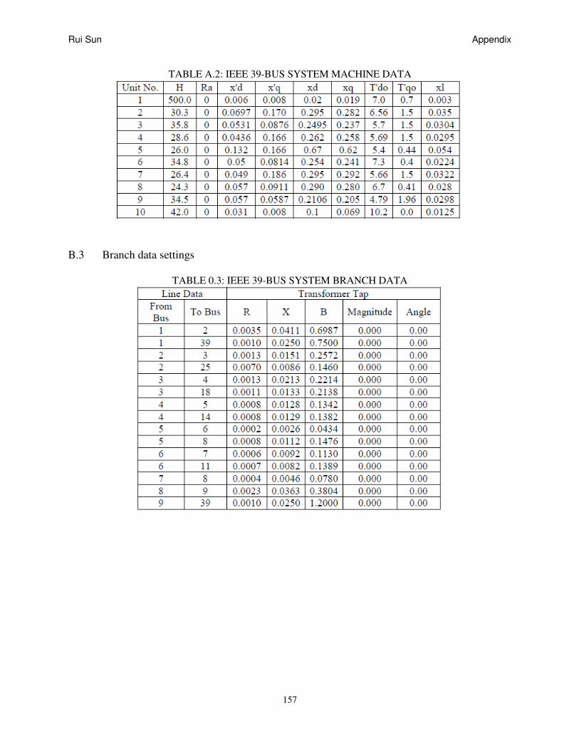
Rui Sun Appendix
157
TABLE A.2: IEEE 39-BUS SYSTEM MACHINE DATA
B.3 Branch data settings
TABLE 0.3: IEEE 39-BUS SYSTEM BRANCH DATA

Rui Sun Appendix
158

Rui Sun Appendix
159
IEEE-30 Bus System
Figure A.2: IEEE 30-Bus System
TABLE A.4: IEEE 30-BUS SYSTEM MACHINE DATA

Rui Sun Appendix
160
TABLE A.5: IEEE 30-BUS SYSTEM BRANCH DATA

Rui Sun Appendix
161
IEEE-57 Bus System
Figure A.3: IEEE 57-Bus System

Rui Sun Appendix
162
IEEE-300 Bus System
Figure A.4: IEEE 300-Bus System

Rui Sun Appendix
163
Appendix C: Matlab Codes for Some of the Algorithms
Islanding Database Initialization
%Main
clear;
clc;
[G,A,Q] = CreateInciM;
%%
BusNum = length(A(1,:));
LineNum = (sum(sum(A))-BusNum)/2;
LineMatrix = zeros(LineNum,2);
t1 = 1;
for k1 = 1:BusNum-1
for k2 = k1+1:BusNum
if(A(k1,k2)==1)
LineMatrix(t1,:) = [k1,k2];
t1 = t1+1;
end
end
end
fprintf('Islanding Analysis')
fprintf('\n')
fprintf('Bus number: ')
fprintf('%3d',BusNum)
fprintf('\n')
fprintf('Line number: ')
fprintf('%3d',LineNum)
fprintf('\n')
%%
MaxTriLine = 2; %Define maximum lines tripped here
%MaxTriLine = LineNum/3;
ObservDepth = 2;
SysObsMat = Nto1(A^ObservDepth,BusNum);
ObsvMatLineNum = (sum(sum(SysObsMat))-BusNum)/2;
ObsvMatLineMatrix = zeros(ObsvMatLineNum,2);
t2 = 1;
for k46 = 1:BusNum-1
for k47 = k46+1:BusNum
if(SysObsMat(k46,k47)==1)
ObsvMatLineMatrix(t2,:) = [k46,k47];
t2 = t2+1;
end
end
end
GLAN = 100;

Rui Sun Appendix
164
Tab1 = zeros(1,MaxTriLine);
Tab2 = zeros(1,BusNum+MaxTriLine+4+GLAN);
fprintf('Islanding Creation & Computation')
fprintf('\n')
T = eye(length(A(:,1)));
for k6 = 1:length(A(:,1))
for k7 = 1:length(A(:,1))
T(k6,k7) = 1;
end
end
count1 = 1;
for k3 = 1:MaxTriLine
fprintf('Trip ')
fprintf('%2d',k3)
fprintf(' line(s)')
fprintf('\n')
if(k3==1)
%Selection = nchoosek(1:LineNum,k3);
for k4 = 1:LineNum%length(Selection(:,1))
C = A;
%for k5 = 1:k3
a1(1,:) = LineMatrix(k4,:);
C(a1(1,1),a1(1,2)) = 0;
C(a1(1,2),a1(1,1)) = 0;
%end
k4
if(mod(count1,100)==0)
count1;
end
[Tab1,Tab2] = IslandComp(BusNum,C,G,T,a1,Tab1,Tab2,MaxTriLine);
count1 = count1+1;
end
else if(k3>1)
ListforT = zeros(1:2);
ListforTset = 1;
for k45 = 901:1100%LineNum
Buss1 = LineMatrix(k45,1);
Buss2 = LineMatrix(k45,2);
SavAslct = zeros(1,2);
savA1 = 1;
PropBus = [Buss1 Buss2];
prpset = 3;
for k48 = 1:ObsvMatLineNum
if(ObsvMatLineMatrix(k48,1)==Buss1||ObsvMatLineMatrix(k48,1)==Buss2)
PropBus(prpset) = ObsvMatLineMatrix(k48,2);
prpset = prpset+1;
else if(ObsvMatLineMatrix(k48,2)==Buss1||ObsvMatLineMatrix(k48,2)==Buss2)
PropBus(prpset) = ObsvMatLineMatrix(k48,1);
prpset = prpset+1;
end

Rui Sun Appendix
165
end
end
for k52 = 1:LineNum
if(ismember(LineMatrix(k52,:),PropBus))
SavAslct(savA1,:) = LineMatrix(k52,:);
savA1 = savA1+1;
end
end
m = length(SavAslct(:,1));
for k63 = 1:m
if(isequal([Buss1 Buss2],SavAslct(k63,:)))
SavAslct(k63:m-1,:) = SavAslct(k63+1:m,:);
break;
end
end
k45
Selection = nchoosek(1:m-1,k3-1);
length(Selection(:,1))
for k51 = 1:length(Selection(:,1))
a1(1,:) = [Buss1 Buss2];
C = A;
C(a1(1,1),a1(1,2)) = 0;
C(a1(1,2),a1(1,1)) = 0;
for k53 = 1:k3-1
a1(k53+1,:) = SavAslct(Selection(k51,k53),:);
C(a1(k53+1,1),a1(k53+1,2)) = 0;
C(a1(k53+1,2),a1(k53+1,1)) = 0;
end
a1 = sortrows(a1);
Duplcotl = 1;
k51
if(ListforTset==1)
ListforT(ListforTset:ListforTset+k3-1,:) = a1;
ListforTset = ListforTset+k3;
[Tab1,Tab2] = IslandComp(BusNum,C,G,T,a1,Tab1,Tab2,MaxTriLine);
count1 = count1+1;
else for k54 = 1:k3:length(ListforT(:,1))
if(isequal(ListforT(k54:k54+k3-1,:),a1))
Duplcotl = 0;
break;
end
end
if(Duplcotl==1)
ListforT(ListforTset:ListforTset+k3-1,:) = a1;
ListforTset = ListforTset+k3;
if(mod(count1,100)==0)
count1
end
[Tab1,Tab2] = IslandComp(BusNum,C,G,T,a1,Tab1,Tab2,MaxTriLine);
count1 = count1+1;
end
end
end
end

Rui Sun Appendix
166
end
end
end
fprintf('----------------')
fprintf('\n')
for k24 = 1:MaxTriLine
fprintf('%1d',k24+1)
fprintf('Islands cases number: ')
fprintf('%3d',Tab1(k24))
fprintf('\n')
end
fprintf('----------------')
fprintf('\n')
fprintf('Different Islands combo: ')
fprintf('%3d',length(Tab2(:,1)))
fprintf('\n')
fprintf('----------------')
fprintf('\n')
for k25 = 1:length(Tab2(:,1))
fprintf('Islands created:')
fprintf('%2d',Tab2(k25,1))
fprintf(' [')
for k26 = 2:MaxTriLine+BusNum+6
if(Tab2(k25,k26)>0)
fprintf('%2d',Tab2(k25,k26))
fprintf(',')
else if(Tab2(k25,k26)==-1&&Tab2(k25,k26+1)~=0)
fprintf(']and[')
else if(Tab2(k25,k26)==-1&&Tab2(k25,k26+1)==0)
fprintf(']')
break;
end
end
end
end
fprintf('\n')
fprintf('Tri_line combo number:')
fprintf('%3d',Tab2(k25,MaxTriLine+BusNum+5))
fprintf(' Base combo:(')
for k27 = MaxTriLine+BusNum+6:2:length(Tab2(1,:))
if(Tab2(k25,k27)>0)
fprintf('%2d',Tab2(k25,k27))
fprintf(' -')
fprintf('%2d',Tab2(k25,k27+1))
fprintf(',')
else if(Tab2(k25,k27)==-1&&Tab2(k25,k27+1)==-1)
fprintf(')')
break;
end
% else if(Tab2(k25,k27)==-1&&Tab2(k25,k27+2)~=0)

Rui Sun Appendix
167
% fprintf(')and(')
% else if(Tab2(k25,k27)==-1&&Tab2(k25,k27+2)==0)
% fprintf(')')
% break;
% end
% end
end
end
fprintf('\n')
fprintf('\n')
end
Incidence Matrix Creation – IEEE-14 Bus System Example
function[G,A,Q] = CreateInciM()
% IEEE-14
Branch14 = [
1 2 0.01938 0.05917 0.0528
1 5 0.05403 0.22304 0.0492
2 3 0.04699 0.19797 0.0438
2 4 0.05811 0.17632 0.0374
2 5 0.05695 0.17388 0.034
3 4 0.06701 0.17103 0.0346
4 5 0.01335 0.04211 0.0128
4 7 0 0.20912 0
4 9 0 0.55618 0
5 6 0 0.25202 0
6 11 0.09498 0.1989 0
6 12 0.12291 0.25581 0
6 13 0.06615 0.13027 0
7 8 0 0.17615 0
7 9 0 0.11001 0
9 10 0.03181 0.0845 0
9 14 0.12711 0.27038 0
10 11 0.08205 0.19207 0
12 13 0.22092 0.19988 0
13 14 0.17093 0.34802 0
];
A = eye(14);
for l1 = 1:length(Branch14(:,1))
A(Branch14(l1,1),Branch14(l1,2)) = 1;
A(Branch14(l1,2),Branch14(l1,1)) = 1;
end
Ld14 = [
1 3 0 0 0 0
2 2 21.7 12.7 0 0
3 2 94.2 19 0 0
4 1 47.8 -3.9 0 0
5 1 7.6 1.6 0 0
6 2 11.2 7.5 0 0
7 1 0 0 0 0

Rui Sun Appendix
168
8 2 0 0 0 0
9 1 29.5 16.6 0 19
10 1 9 5.8 0 0
11 1 3.5 1.8 0 0
12 1 6.1 1.6 0 0
13 1 13.5 5.8 0 0
14 1 14.9 5 0 0
];
Gen14 = [
1 232.4 -16.9 10 0 1.06 332.4 0
2 40 42.4 50 -40 1.045 140 0
3 0 23.4 40 0 1.01 100 0
6 0 12.2 24 -6 1.07 100 0
8 0 17.4 24 -6 1.09 100 0
];
for l1 = 1:length(Gen14(:,1))
G(1,l1) = Gen14(l1,1);
end
Q = 10;
Islanding Contingency Detecting Stratgy
function [Tab1,Tab2] = IslandComp(BusNum,C,G,T,a1,Tab1,Tab2,MaxTriLine)
Cb = C;
for iteration = 2:BusNum
C1 = C;
C = Nto1(C*Cb,BusNum);
if(isequal(C,T))
Tab1 = Tab1;
Tab2 = Tab2;
return;
end
if(isequal(C1,C))
Islandgroup = zeros(length(a1(:,1))+1,BusNum);
Islandgroup(1,1) = 1;
GroupNum = 1;
Grouplength = zeros(length(a1(:,1))+1,1);
Grouplength(1,1) = 1;
for k8 = 2:BusNum
set = 1;
for k9 = 1:GroupNum
for k10 = 1:Grouplength(k9,1)
if(C(Islandgroup(k9,k10),k8)==1)
Grouplength(k9,1) = Grouplength(k9,1)+1;
Islandgroup(k9,Grouplength(k9,1)) = k8;

Rui Sun Appendix
169
set = 0;
break;
end
end
if(set==0)
break;
end
end
if(set==1)
GroupNum = GroupNum+1;
Grouplength(GroupNum,1) = Grouplength(GroupNum,1)+1;
Islandgroup(GroupNum,1) = k8;
end
end
IslandNum = GroupNum;
sign = 1;
badpart = 0;
for k14 = 1:GroupNum
test = 1;
for k15 = 1:Grouplength(k14,1)
for k16 = 1:length(G)
if(G(k16)==Islandgroup(k14,k15))
test = 0;
break;
end
end
if(test==0)
break;
end
end
if(test==1)
IslandNum = IslandNum-1;
badpart(sign) = k14;
sign = sign+1;
end
end
if(IslandNum>1)
Islandgroup_2 = Islandgroup;
if(IslandNum<GroupNum)
for k18 = 1:length(badpart)
Islandgroup_2(badpart(k18):length(a1(:,1)),:) = Islandgroup_2(badpart(k18)+1:length(a1(:,1))+1,:);
end
Islandgroup_2(length(a1(:,1))+2-length(badpart):length(a1(:,1))+1,:) = 0;
end
zhizhen1 = 1;
Save = zeros(1,BusNum+MaxTriLine+1);
for k19 = 1:IslandNum
for k20 = 1:BusNum
if(Islandgroup_2(k19,k20)~=0)
Save(zhizhen1) = Islandgroup_2(k19,k20);
zhizhen1 = zhizhen1+1;
end

Rui Sun Appendix
170
end
Save(zhizhen1) = -1;
zhizhen1 = zhizhen1+1;
end
zhizhen2 = 1;
for k21 = 1:length(a1(:,1))
Save2(1,zhizhen2:zhizhen2+1) = a1(k21,:);
zhizhen2 = zhizhen2+2;
end
Save2(1,zhizhen2:zhizhen2+1) = [-1,-1];
Tab1(1,IslandNum-1) = Tab1(1,IslandNum-1)+1;
if(Tab2(1,1)==0)
Tab2(1,1) = IslandNum;
Tab2(1,2:MaxTriLine+BusNum+2) = Save;
Tab2(1,MaxTriLine+BusNum+5) = 1;
Tab2(1,MaxTriLine+BusNum+6:MaxTriLine+BusNum+5+length(Save2)) = Save2(1,:);
else
judge2 = 1;
for k22 = 1:length(Tab2(:,1))
if(Tab2(k22,1)~=0)
if(isequal(Save,Tab2(k22,2:MaxTriLine+BusNum+2)))
Tab2(k22,MaxTriLine+BusNum+5) = Tab2(k22,MaxTriLine+BusNum+5)+1;
for k23 = MaxTriLine+BusNum+6:length(Tab2(1,:))
if(Tab2(k22,k23-1)==-1&&Tab2(k22,k23)==0)
Tab2(k22,k23:k23+length(Save2)-1) = Save2(1,:);
Tab2(k22,length(Tab2(k22,:))+1) = 0;
judge2 = 0;
break;
end
end
end
if(judge2==0)
break;
end
end
end
if(judge2==1)
Tab2(length(Tab2(:,1))+1,1) = IslandNum;
Tab2(length(Tab2(:,1)),2:MaxTriLine+BusNum+2) = Save;
Tab2(length(Tab2(:,1)),MaxTriLine+BusNum+5) = 1;
Tab2(length(Tab2(:,1)),MaxTriLine+BusNum+6:MaxTriLine+BusNum+5+length(Save2)) = Save2(1,:);
end
end
end
return;
end
end

Rui Sun Appendix
171
Boolean Conversion
function [A] = Nto1(A,BusNum)
for i = 1:BusNum
for j = 1:BusNum
if(A(i,j)~=0)
A(i,j) = 1;
end
end
end
Non-Islanding Cases Generation
BUS138_115 = [
….
];
t1 = randperm(length(BUS138_115));
t1 = t1(1,1:100);
for i = 1:100
RdmFltBus(i,:) = BUS138_115(t1(i),:);
end
------
Triporder = [
……
];
Trip_havingLD = [
……
];
T = length(Trip_havingLD(:,1));
T2 = length(Triporder(:,1));
flag1 = 1;
for r1 = 1:T
for r2 = 1:T2
if(Trip_havingLD(r1,:)==Triporder(r2,1:4))
KeepTrip(flag1,1) = r2;
flag1 = flag1+1;
end
end
end
KeepTrip = sort(KeepTrip);

Rui Sun Appendix
172
Curve Fitting for ISI
%% Islanding curve fitting
AA = [
…..
];
for num = 10:10
BB = Islandingcurvefitting(:,num);
[a1,b1] = Curvefitting1(AA,BB);
A(num,1) = a1.a;
B(num,1) = a1.b;
C(num,1) = a1.c;
D(num,1) = a1.d;
E(num,1) = a1.e;
end