Why the Major Field (Business) Test Does Not Report Subscores of

Individual Test-takers—Reliability and Construct Validity Evidence

Guangming Ling

ETS, Princeton, NJ

Paper presented at the annual meeting of the American Educational Research Association (AERA) and the

National Council on Measurement in Education (NCME)

April 13-17, 2009, San Diego, CA.

Unpublished Work Copyright © 2009 by Educational Testing Service. All Rights Reserved. These materials are an unpublished, proprietary work of ETS. Any limited distribution shall not constitute publication. This work may not be reproduced or distributed to third parties without ETS's prior written consent. Submit all requests through www.ets.org/legal/index.html.

Educational Testing Service, ETS, the ETS logo, and Listening. Learning. Leading. are registered trademarks of Educational Testing Service (ETS).

i

Abstract

The current study evaluated whether to report individual test-takers’

subscores of the Major Field Business Test (MFT Business) by analyzing subscores’

reliabilities and the internal structure of the test. Reliability analysis found that for

each individual student, the observed subscores did not contribute statistically

meaningful information beyond the total score of the test. In addition, analysis of

internal structure of the MFT Business found a uni-dimensional construct to be

present, which also did not support the additional reporting of subscores for each

individual student. The relationship between the two analyses was also discussed

and an alternate method was recommended for future research. The study

concluded that the MFT Business should not report subscores of individual

students.

1

Introduction

Reporting scores on the subscales (or sub-domains) of a test may provide test-

takers and test users with better knowledge of test performance on a sub-domain or a

subset of items, especially when the sub-domains of a test vary by content or underlying

construct. For example, an exit test for undergraduate business majors may contain items

related to different aspects of business knowledge, including knowledge of accounting,

economics, management, quantitative and information systems, finance, marketing, and

legal and social environment. In addition to the total test score, students or teachers may

also be interested in knowing examinees’ competence in each aspect of the curriculum.

In recent years, there have been increasing demands for the reporting of subscores,

especially subscores of individuals. In their review, Goodman and Hambleton (2004)

found that all of the states and companies being reviewed, including two Canadian

provinces, eleven U.S. states, and three U.S. testing companies, provided certain

information on the sub-domain level (i.e. subscores of individual students). Not

surprisingly, test-takers and score users of the Major Field Test of Business (MFT

Business) are also requiring more information from the test, including subscores of

individual students in addition to the total test score.

MFT Business is a comprehensive outcomes assessment of basic, critical

knowledge obtained by students in a business major (for an associate, bachelor, or MBA

degree). Students typically take the Major Field Tests after they successfully complete

the major-required courses. The total test scores of individuals are reported on a scale of

120–200 (the MBA test has a scale of 220–300). The MFT Business, like MFT of other

majors, also reports subscores (on a scale of 20–100) at aggregate levels (e.g. the average

2

subscore of a class or a program) in subfields of the discipline (ETS, 2008). The

subscores of MFT Business at the institutional level are used to indicate mastery of

business knowledge as a group (i.e., as a class or a program) instead of an individual

student. However, the MFT Business does not report subscores of individual students.

In order to report the subscores to individual students1, several steps are required

during the test development procedure. For example, it is necessary to ensure that each

content or domain area is well and equally (or proportionally) represented, each subscale

has similar and sound psychometric properties (e.g., with equal or comparable high

reliabilities).

When a test was not designed to report subscores of individual students, a post

hoc evaluation is necessary. Different methods and perspectives need to be considered in

evaluating this issue. There have been debates on whether to report subscores and under

what conditions. Ferrara & DeMauro (2007) recommended that a subscore to be reported

if it has a high reliability (i.e., an internal consistency reliability estimate of .85 or higher)

and does not highly correlate with other subscores; a subscore with a low reliability

should not be reported. On the other hand, subscores of different content areas, sub-

domains, etc., are in great demand by stakeholders (Haladyna & Kramer, 2004)

regardless of the original purpose when the test was first developed. Test-takers want to

know about their strengths and weaknesses in different content areas for future

improvement; teachers, deans, and institutions want to know test performance on various

sub areas to make necessary improvement to programs’ curricula.

1 In this paper, subscore, if not specified, stands for the subscore of individual students.

3

The internal structure of the MFT Business may also need to be considered in

addition to subscores’ reliabilities. The internal structure of the test could provide

information such as what sub-constructs or sub-contents are implied in the test design,

how they are measured, and what the inter-relationships are. Understanding the internal

structure would help to interpret the test scores as well as the subscores. For example, if

the MFT Business presents a multidimensional structure, it may support the reporting of

individuals’ subscore of each dimension.

The current study aimed to address three research questions:

1. Do subscores of individual students add information to the total score

statistically?

2. What is the internal structure of the MFT Business? Does the internal

structure support the reporting of content-related subscores of individual students?

3. Are the answers to these two questions consistent with one another?

Methods

Instrument and Data

The data came from the MFT Business test administered between 2002 and 2006.

There were 155,921 students who took the test during this time period. Students with

incomplete records were excluded from the analysis and a final number of 155,235

students were included in this study. The test included 118 multiple choice items from

4

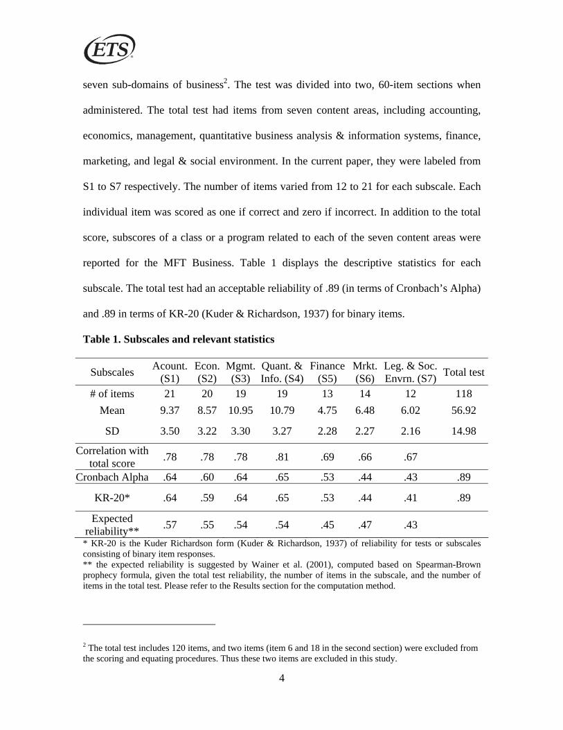
seven sub-domains of business2. The test was divided into two, 60-item sections when

administered. The total test had items from seven content areas, including accounting,

economics, management, quantitative business analysis & information systems, finance,

marketing, and legal & social environment. In the current paper, they were labeled from

S1 to S7 respectively. The number of items varied from 12 to 21 for each subscale. Each

individual item was scored as one if correct and zero if incorrect. In addition to the total

score, subscores of a class or a program related to each of the seven content areas were

reported for the MFT Business. Table 1 displays the descriptive statistics for each

subscale. The total test had an acceptable reliability of .89 (in terms of Cronbach’s Alpha)

and .89 in terms of KR-20 (Kuder & Richardson, 1937) for binary items.

Table 1. Subscales and relevant statistics

Subscales Acount. (S1)

Econ. (S2)

Mgmt.(S3)

Quant. &Info. (S4)

Finance(S5)

Mrkt.(S6)

Leg. & Soc. Envrn. (S7) Total test

# of items 21 20 19 19 13 14 12 118 Mean 9.37 8.57 10.95 10.79 4.75 6.48 6.02 56.92

SD 3.50 3.22 3.30 3.27 2.28 2.27 2.16 14.98

Correlation with total score .78 .78 .78 .81 .69 .66 .67

Cronbach Alpha .64 .60 .64 .65 .53 .44 .43 .89

KR-20* .64 .59 .64 .65 .53 .44 .41 .89

Expected reliability** .57 .55 .54 .54 .45 .47 .43

* KR-20 is the Kuder Richardson form (Kuder & Richardson, 1937) of reliability for tests or subscales consisting of binary item responses. ** the expected reliability is suggested by Wainer et al. (2001), computed based on Spearman-Brown prophecy formula, given the total test reliability, the number of items in the subscale, and the number of items in the total test. Please refer to the Results section for the computation method.

2 The total test includes 120 items, and two items (item 6 and 18 in the second section) were excluded from the scoring and equating procedures. Thus these two items are excluded in this study.

5

Methods and Analyses

Wainer et al. (2001) suggested using an augmented score—borrowing strength

from other items in the test to compute the subscore of a given student — to improve the

subscore’s reliability. Wainer’s augmented scores could be treated as a special case of the

several indices suggested by Haberman (2005; Haberman, Sinharay, & Puhan, 2006;

Sinharay, Haberman & Puhan, 2006). Haberman suggested that reliability-based analysis

may help to inform the decision of subscore reporting. Haberman’s approach compared

the mean-squared-error (MSE) of true subscore when it was predicted (or approximated)

by the observed subscale score, the observed total test score, and the two scores

conjointly. The rationale is that if the MSE of the true subscore is smaller than the MSE

implied by other models or estimations, then the observed subscore contributes

something unique and substantial in addition to the total score. Otherwise, it only

provides redundant information statistically, since the same level of information could

have been obtained from the observed total test score with less error.

Descriptive analyses of item scores, subscores, and total test scores were

conducted. Moreover, the reliability of each subscale, the total test, the correlations

between subscores, and the correlations between each subscore and the total test score

were analyzed and compared. Following the approach of Haberman (2005) and his

colleagues, MSE’s of the true subscores were computed and compared for the seven

subscales respectively.

It should be noted that the reliability-based approach failed to take into account

the internal structure of the test. In many cases, the dimensionality of a test may influence

the interpretation of the subscore and impact the decision of reporting subscores of

6

individual students as well. Analyzing the internal structure (or dimensionality) of the test

and subscales may provide additional evidence over the reliability analysis.

Factor analysis and structural equation modeling were applied to evaluate the

internal structure of the MFT Business. Traditional factor analysis extracts factors from a

set of continuous observed variables by assuming a subset of variables representing a

latent factor (or construct). However, such an approach may lead to a biased estimation

of the latent construct and other parameters when the observed variables are categorical

or binary. More contemporary factor analysis methods were developed in the last three

decades, typically for categorical or binary variables (i.e., item responses in the form of

true or false, or in a Likert scale). Woods (2002) summarized the difference between

traditional factor analysis based on continuous observed variables and more

contemporary factor analysis based on categorical (binary) variables. He suggested that

the application of traditional factor analysis to binary item scores can lead to biased

estimation of the standard errors, biased significance tests, overestimation of the number

of factors, and underestimation of the factor loadings.

Two general methods were developed to link the item responses (categorical or

binary responses) and the underlying latent factor/construct: the probit linking function

(limited information approach, Joréskög, 1999) and the logit linking function (full

information approach, Bock & Aitkin, 1981). The models using the probit linking

function were basically under the framework of structural equation modeling (SEM),

which was first developed by Joréskög and later by Muthén and others (Muthén and

Muthén, 1998, in MPLUS; LISREL, Joréskög, 1999; and EQS, Bentler, 2001). The

model was typically fitted to the tetrachoric/polychoric correlation matrix, and was

7

generally called the limited information factor analysis (LIFA). On the other hand, a logit

approach was taken and used in logistic IRT models (named as item factor analysis or

full3 information item factor analysis (FIFA; Bock & Aitkin, 1981; Bock, Gibbons, &

Muraki, 1988; Takane & De Leeuw, 1987; Wood, Wilson, Gibbons, Schilling, Muraki, &

Bock, 1991).

Both approaches assume that a continuous and normally-distributed latent

variable is underlying the observed dichotomous or categorical responses. TESTFACT

(Wilson, Wood, & Gibbons, 1991) is a factor analysis program that is typically used for

binary scored items based on the tetrachoric correlations and the full information–item-

factor–analysis (FIFA). It computes the maximum likelihood estimates of parameters via

the expectation-maximization algorithm (Bock & Aitkin, 1981; Bock & Lieberman,

1970; Dempster, Laird, & Rubin, 1977), which provides a significance test for the change

of number of factors. Other analytic tools have been developed using the logit approach,

such as MULTILOG (Thissen, 1991), and ConQuest (Wu, Adams, & Wilson, 1998;

Wang, 1995; Adams, Wilson, & Wang, 1997). However, the FIFA approach requires a

large sample size relative to the number of items ( 2n for n binary items) to obtain a

reasonable frequency for all possible response patterns. For example, when there are only

2 binary items, there will be four ( 22 ) possible patterns, 00, 01, 10, and 11. The sample

size should be at least four in order to have all the possible patterns occur (du Toit, 2003).

In order to have all the possible unique patterns of the 118 binary items, the sample size

needs to be at least 1182 . Unfortunately, the sample size we have in this study is only

3 “Full” means using all the item level responses information, comparing to analysis only based on the correlation /covariance matrix.

8

155,235 (between 172 and 182 ), which is much smaller than required. Thus, the FIFA

approach was not considered in this study. A major concern was that the sample size was

not big enough relative to the number of items (118).

Two levels of exploratory analysis were conducted to evaluate the internal

structure of the test: One was based on the variances and covariances matrix of observed

subscores, and the other was based on the tetrachoric correlation matrix of the item

scores. Traditional factor analysis (both principal component analysis and the exploratory

factor analysis based on maximum likelihood method) was performed based on the

variance-covariance matrix of the seven subscale scores (assumed as continuous

variables). Confirmatory factor analysis was then performed based on the variance-

covariance matrix of subscale scores.

The more contemporary factor analysis (both exploratory and confirmatory) was

performed based on the binary item scores (the tetrachoric correlation matrix). The

purpose was to examine three questions: How well each subscale was measured by a

subset of items related to a sub-domain of business knowledge; How the general

knowledge and skills of the business majors were measured by the 118 items; And how

the seven subscales were structured to each other.

Four models were examined based on the item scores. First, a single factor

measurement model was fit to the data for all items, examining whether all 118 items

measured a single factor. Second, a measurement model was examined for each subscale

based on the binary item scores for each of the seven subscales. The purpose was to

examine how the items of the same sub-domain performed when they were set to

measure a common latent construct. Third, a full structural equation model, including all

9

the seven subscales, was fit to the data, with all the subscale-related latent variables inter-

correlated. The fourth model had the same seven subscales as the third model, with a

second order common factor extracted from the seven latent variables. All the four

models were based on the probit linking function between the binary item score and the

underlying latent variable. The analyses were based on the tetrachoric correlation matrix

of the binary scores, applying the diagonal weighted least square (DWLS) estimation

method through LISREL 8.8 (Joréskög & Sorbom, 1999).

Results

Results of Descriptive Analysis and Reliability Analysis

Descriptive results showed that the reliability of each subscale (Cronbach’s Alpha

coefficient) ranged from .43 to .65, which were much lower than the total test reliability

(.89). These subscale reliabilities would be considered low according to the commonly

accepted value of .70 in psychological and educational measurement (Nunnally &

Bernstein, 1994, pp. 265). Similar low values of reliabilities were found for each subscale

using the KR-20 formula (Kuder & Richardson, 1937). The expected reliability4 of each

subscale was also computed using the Spearman-Brown formula given the total test

reliability (Nunnally & Bernstein, 1994). The expected reliabilities were generally lower

4 Expected subscale reliability of a given subscale ( sρ ) is calculated based on the Spearman-Brown formula, given the number of items in the total test (K), the number of items in the subscale (k), and the total test reliability ρ .

ρ =( / )*

1 ( / 1)*s

s

K kK k

ρρ+ −

(See Nunnally & Bernstein, 1994; Wainer, et al., 2001).

10

than the actual reliabilities across the seven subscales, which supports a unidimensional

model for the test (Wainer, et al, 2001).

Following Haberman and his colleagues’ (2005; Sinharay, Haberman & Puhan,

2006) approach, four sets of MSEs were computed and compared to the MSE of the true

subscore when it was estimated from the observed subscore –SD(Se). The four sets of

mean square errors were computed based on the regression of the true subscore on the

observed total score—SD(L-St), on the observed total score and the subscore—SD(M-

St), on the Kelly’s estimation of true subscore—SD(K-St), and the approximated true

error of subscore—SD(F-Dt). It was expected that the SD(Se) be the smallest if the

subscore provided substantial information in addition to the total test score. However,

results showed that the MSE of the true subscale score estimated from the observed

subscale score was consistently greater than those estimated from the observed total

score, the combination of the subscale score and the total score, and the approximated

true MSE (See Table 2).

Using the first subscale S1-accounting as an example, the SD(Se) for S1 was 2.09,

which represented the standard error of the true subscore of S1 when it was predicted

from the observed subscore. The standard error for the observed total score SD(L-St) was

only 1.38, which was much smaller (See Table 2). This suggested that the prediction of

subscale S1’s true score from the observed subscore produced more error than it did from

the total test observed score. Similarly, we found the MSEs of the other predictors or

approximation methods were all smaller than that of the observed S1 subscore. The same

results were found in the other six subscales (see Table 2); the true subscore’s MSE was

greater when it was predicted by the observed subscore than those with other predictors.

11

These results suggested that the observed subscore of a given student provided similar if

not redundant information over the total test score but at a less reliable level.

Table 2. Mean square error comparisons using Haberman’s (2005) approach

Subscale S1 S2 S3 S4 S5 S6 S7

#Items 21 20 19 19 13 14 12

SD(Se) 2.09 2.05 1.99 1.93 1.56 1.70 1.66

SD(K-St) 1.67 1.58 1.59 1.56 1.14 1.12 1.06

SD(L-St) 1.38 1.06 1.25 1.06 0.86 0.64 0.58

SD(M-St) 1.53 1.39 1.44 1.40 0.97 0.88 0.83

SD(F-Dt) 1.67 1.58 1.59 1.56 1.14 1.12 1.06

Note: S stands for subscale observed score, sub-note t stands for the true score respectively; sub-note e

stands for the measurement error in classical test theory; E( ) stands for the expected value or average;

SD( ) stands for the standard deviation; Dt is the approximated true residual defined by Haberman

(2005);

SD(Se) is the mean standard deviation of measurement error (or the regression residual when using

observed subscale score to predict the subscale true score St;

SD(K-St) stands for the mean-squared error of regression when using K to predict the subscale true score

St (K is the Kelly approximation of St);

SD(L-St) stands for the mean-squared error of regression when using the observed total test score to

predict the subscale true score St (L is the predicted St from the total observed score);

SD(M-St) stands for the mean-squared error of regression when using the observed subscale score S and

the observed total test score X together to predict the subscale true score St;

SD(F-Dt) stands for the mean-squared error of regression when using F to predict the true residual Dt (F is

an approximation of the true residual Dt, see Haberman, 2005).

12

Results of Subscale Score Factor Analysis

Exploratory factor analysis (EFA) was conducted based on the variance-

covariance matrix of the seven observed subscores (number of correct raw scores).

SAS9.1 (SAS INC., 2002) was used for the EFA. The screeplot in Figure 1 suggests that

one or two dimensions may represent the seven observed subscores at an acceptable

level. A clear elbow was present at the second factor, with 54% of the total variance

explained by the first factor, and 65% by the first two factors.

‚ 1 3.0 ˆ E 2.5 ˆ i 2.0 ˆ g ‚ e 1.5 ˆ n ‚ v ‚ a 1.0 ˆ l ‚ u 0.5 ˆ e ‚ 2 s 0.0 ˆ 3 ‚ 4 5 6 7 -0.5 ˆ ˆƒƒƒƒƒƒƒƒƒˆƒƒƒƒƒƒƒƒƒˆƒƒƒƒƒƒƒƒƒˆƒƒƒƒƒƒƒƒƒˆƒƒƒƒƒƒƒƒƒˆƒƒƒƒƒƒƒƒƒˆƒƒƒƒƒƒƒƒƒˆƒ 0 1 2 3 4 5 6 7

Figure 1.

Screeplot of eigenvalues

The factor loadings for the one-factor and the two-factor models based on

maximum likelihood estimation method are presented and compared in Table 3. The

subscales’ loadings on the single factor were relatively high, ranging from .61 to .76. For

the two-factor structure (after PROMAX rotation), four subscales (S2, S3, S4, S6 and S7)

had a substantial loading on the first factor, while the remaining two subscales (S1 and

13

S5) together with subscales S2 and S4 had a substantial loading on the second factor. It

seemed that the two factors are not clearly interpretable. The second factor seemed to be

related to quantitative knowledge, but the subscale of quantitative and information system

also had high loadings on the first factor. The first factor seemed to be related to less

quantitative business concepts or theories.

Table 3. Factor loadings for 1-factor and 2-factor models

1-factor 2-factor before rotation

2-factor after PROMAX

rotation Number

of items1 1 2 1’ 2’

S1-accounting 21 .71 .71 -.12 .21 .54

S2-economic 20 .72 .72 -.06 .30 .46

S3-management 19 .72 .72 .15 .62 .15

S4-Quantitative & Information system 19 .76 .76 .01 .43 .38

S5-finance 13 .64 .64 -.18 .09 .59

S6-marketing 14 .63 .63 .09 .48 .19

S7-Legal & Social Environment 12 .61 .61 .11 .50 .14

Given that the second factor’s eigenvalue was less than one and the two factors

was difficult to interpret, only the one-factor model was examined in the next stage of

confirmatory factor analysis. The factor loadings below .2 were omitted (fixed as zero) in

the model specification. The model was fitted to the data using LISREL 8.8 (Joréskög,

1999). The fit indices suggests that the model fitted the data acceptably well. The root

mean square error of approximation (RMSEA) value was .064, the comparative fit index

(CFI) value was .99, the Tucker-Lewis Index (TLI) value was .98, the standardized root

mean square residual (SRMR) value was .024, and the Chi-square value was 8851

14

(p<.000; see Figure 2). The subscale S4 (quantitative and information systems) was the

strongest indicator of the latent trait of business field knowledge, with the highest

standardized loading (.78). The subscale S7 (legal and social environment) was a

relatively weak indicator with the lowest standardized loading (.62). The well-fitted

model suggested the uni-dimensionality of the MFT Business.

Figure 2.

Factor structure for one -factor model at subscale level.

Results of Item Level Factor Analysis

A measurement model with a single latent variable indicated by a subset of binary

items was constructed and analyzed for each of the seven subscales. The single factor

measurement model fitted the data well for each subscale (see Table 3). All the RMSEAs

were below the .05 criterion and some of them were very close to .01, which suggested

that the distances between the model-implied correlation matrix and the tetrachoric

correlation matrix was very small (Hu & Bentler, 1999). The CFIs and TLIs were all

15

above .98, which could be considered a good fit between the model and the data.

Although they were all significantly different from zero (at .05 level), there were items

with relatively low loadings within each subscale. For example, Items-4 and -86 of S1-

accounting; Items-94, -103, and -107 of S2-economics; Items-25 of the S3-management;

Items-30 of S5-finance; Item-68 of S6-marketing; Items-18, -52, and -104 of S7-legal and

social environment had low factor loadings below .2. A further examination found that all

the low-loading items (except Items-25 and -30) overlapped with the low-loading items

found in a one-factor measurement model for all the 118 items (see the next section for

details).

Table 4. Model fit indices for the subscales’ measurement models.

A single factor measurement model was then fit to the tetrachoric correlation

matrix of all the 118 binary items. All 118 items in the test were loaded on the single

common factor, which can be treated as a measurement model for all items of the test.

The results suggested that the single factor model for all items fit the data at an

acceptable level, with the RMSEA value of .015, the SRMR value of .025, the CFI value

of .903, and the TLI value of .959. The item-factor loadings were all significantly

Subscale Name RMSEA 90%CI RMSEA TLI CFI

S1-Accounting .015 (.014,.017) .99 .99

S2-Economics .016 (.014,.017) .99 .99

S3-Management .015 (.013,.016) .99 .99

S4-Quantitative & Information systems .020 (.019,.021) .99 .99

S5-Finance .016 (.014,.019) .99 .99

S6-Marketing .014 (.012,.016) .98 .98

S7-Legal & Social Environment .014 (.011,.016) .99 .99

16

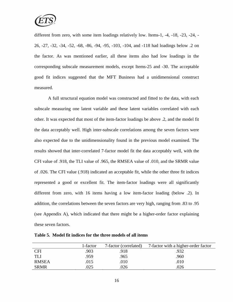
different from zero, with some item loadings relatively low. Items-1, -4, -18, -23, -24, -

26, -27, -32, -34, -52, -68, -86, -94, -95, -103, -104, and -118 had loadings below .2 on

the factor. As was mentioned earlier, all these items also had low loadings in the

corresponding subscale measurement models, except Items-25 and -30. The acceptable

good fit indices suggested that the MFT Business had a unidimensional construct

measured.

A full structural equation model was constructed and fitted to the data, with each

subscale measuring one latent variable and these latent variables correlated with each

other. It was expected that most of the item-factor loadings be above .2, and the model fit

the data acceptably well. High inter-subscale correlations among the seven factors were

also expected due to the unidimensionality found in the previous model examined. The

results showed that inter-correlated 7-factor model fit the data acceptably well, with the

CFI value of .918, the TLI value of .965, the RMSEA value of .010, and the SRMR value

of .026. The CFI value (.918) indicated an acceptable fit, while the other three fit indices

represented a good or excellent fit. The item-factor loadings were all significantly

different from zero, with 16 items having a low item-factor loading (below .2). In

addition, the correlations between the seven factors are very high, ranging from .83 to .95

(see Appendix A), which indicated that there might be a higher-order factor explaining

these seven factors.

Table 5. Model fit indices for the three models of all items

1-factor 7-factor (correlated) 7-factor with a higher-order factor CFI .903 .918 .932 TLI .959 .965 .960 RMSEA .015 .010 .010 SRMR .025 .026 .026

17

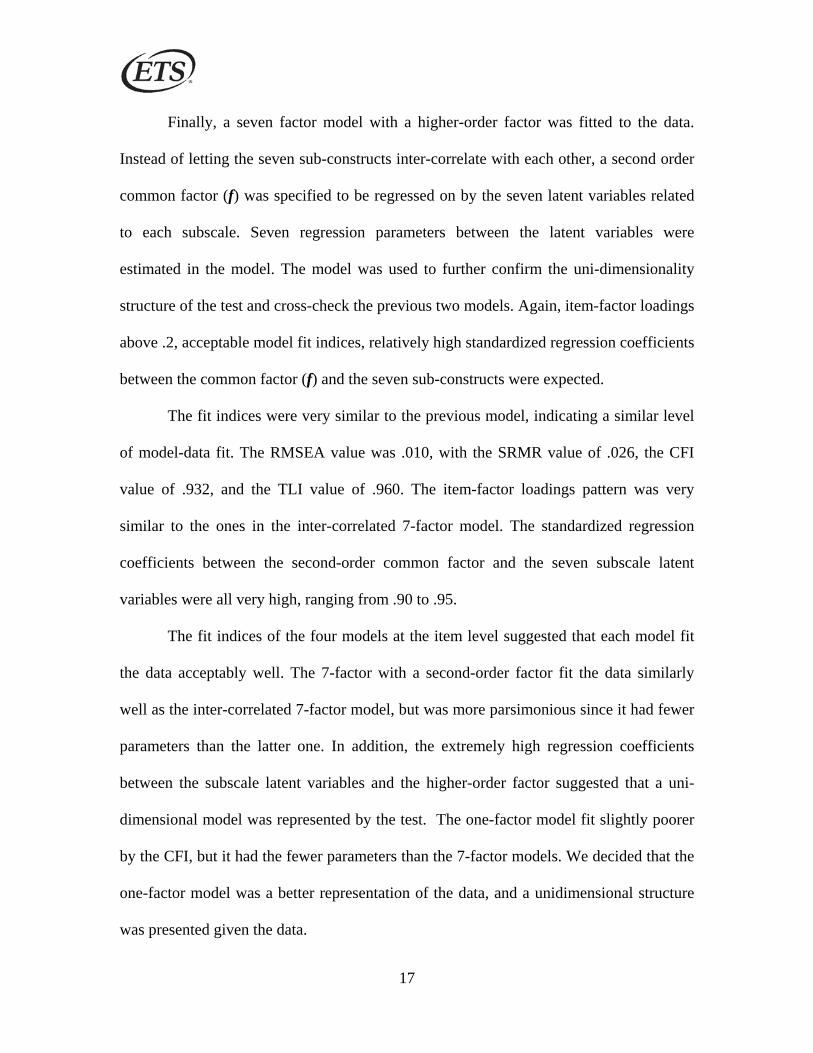
Finally, a seven factor model with a higher-order factor was fitted to the data.

Instead of letting the seven sub-constructs inter-correlate with each other, a second order

common factor (f) was specified to be regressed on by the seven latent variables related

to each subscale. Seven regression parameters between the latent variables were

estimated in the model. The model was used to further confirm the uni-dimensionality

structure of the test and cross-check the previous two models. Again, item-factor loadings

above .2, acceptable model fit indices, relatively high standardized regression coefficients

between the common factor (f) and the seven sub-constructs were expected.

The fit indices were very similar to the previous model, indicating a similar level

of model-data fit. The RMSEA value was .010, with the SRMR value of .026, the CFI

value of .932, and the TLI value of .960. The item-factor loadings pattern was very

similar to the ones in the inter-correlated 7-factor model. The standardized regression

coefficients between the second-order common factor and the seven subscale latent

variables were all very high, ranging from .90 to .95.

The fit indices of the four models at the item level suggested that each model fit

the data acceptably well. The 7-factor with a second-order factor fit the data similarly

well as the inter-correlated 7-factor model, but was more parsimonious since it had fewer

parameters than the latter one. In addition, the extremely high regression coefficients

between the subscale latent variables and the higher-order factor suggested that a uni-

dimensional model was represented by the test. The one-factor model fit slightly poorer

by the CFI, but it had the fewer parameters than the 7-factor models. We decided that the

one-factor model was a better representation of the data, and a unidimensional structure

was presented given the data.

18

Summary and Discussions

In summary, the study found that the observed subscores of the MFT Business

correlated moderately with each other, and correlated moderately to highly with the

observed total test score. Each subscale had a relatively lower level of reliability than the

total test. The low reliabilities of the seven subscales and the small differences between

the expected reliability and the observed reliability indicated that the test might be very

likely uni-dimensional (Wainer, et al, 2001). The correlations between the observed

subscores and the total score were greater than the subscales’ reliabilities, which

suggested that the construct measured by the total test is more reliable than that measured

by the subscales.

Analysis using Haberman’s (2005) approach found that the MSE of the subscale

true score was greater when estimated by the observed subscores than when estimated by

the total observed score or other predictors. In other words, the subscale true score

estimated by the subscale observed score was less reliable than the ones estimated by the

total test observed score. These results supported the claim that reporting subscores of

individual students may not add statistically meaningful information to the total score.

Traditional factor analysis on the subscores suggested that a one-factor model fit

the data well. The item factor analysis based on the probit linking function found that a

one-factor model fitted the data acceptably well. These results suggested that although

there might be content-related constructs measured by each subscale, but statistically

there was a unidimensional constructed presented in the MFT Business given the data.

Combining the results from both reliability analysis and the factor analysis on the

internal structure, we think that the MFT Business should not provide subscores of

19

individual students since it could not add meaningful information statistically over the

total test score.

Relationship between Haberman’s (2005) approach and the factor structure

There might be a relationship between the two approaches applied in this study.

The method suggested by Haberman (2005) and his colleagues extended the reliability

concept in classical test theory by regressing the subscale true score on the total test

observed score or a combination of observed subscore and observed total score. Such

extensions might implicitly require that the subscale and the total test measure the same

construct. That is, even though the test consists several subscales or content domains, it

measures a unidimensional construct. In a unidimensional test, the total test observed

score is always a more reliable measure of the true score (with less error) than any subset

of items in the test. In other words, the subscore’s correlation with the subscale true score

would always be lower than its correlation with the total test true score. For a

multidimensional test where subscales measure more distinct sub-constructs that are

correlated at a low or moderate level, the reliability of subscale might be more

comparable to or even higher than its correlation with the total test true score. In such

cases, the inter-correlations between the subscales would be relatively low or moderate,

and the total test reliability might be lower than the subscale’s reliability. If one followed

the same criteria proposed by Haberman and his colleagues (2005) for such cases and

neglected the internal structure of the test, the conclusions and inferences would be

misleading.

Even in cases of unidimensional tests, a criterion or subjective decision on an

acceptable reliability might be required; that is, how reliable the subscore should be in

20

order to be reported. If following Ferrara & DeMauro’s (2007) suggestion of .85 as the

rule of thumb, all seven subscales of MFT Business failed to satisfy the criterion and

should not be reported. However, this requirement might be too high for general

educational and psychological tests. In psychological tests and some achievement tests, a

measure with an internal consistency of .7 or higher was generally considered reliable

(Nunnally & Bernstein, 1994). A minimum level of reliability could ensure the

measurement quality and reduce the difficulty in deciding whether to report subscores

related to a domain or content area. If the subscale itself cannot provide a reliable

measure of the sub-construct (e.g., with a Cronbach’s alpha value below .7) and the

subscores of individual students were decided to be reported, one might need to borrow

information from other subscales or the total test in order to obtain a more reliable

measure. In such a case, we might need to make sure that the construct measured by the

subscale in question and the construct measured by the other subscales should be the

same or similar.

Although the subscales of MFT Business refer to specific content areas, knowing

the weakness or strength related to a content area might not be very helpful if the test is

designed as a unidimensional test. On the one hand, the construct or ability measured by

a subset of items may not necessarily be content specific; rather, it may be an ability

shared by the other subscales. On the other hand, content-specific related subscores could

be misleading if they were reported and used to inform decisions related to curriculum

reform or re-design, given the fact that subscores have relatively low reliability and have

not been validated for such purposes.

21

In conclusion, the study demonstrated that in deciding whether to report subscores

of individual students, the reliability analysis approach (Haberman, 2005) is more

convincing when combined with construct validity evidence. The fact is that most

educational tests were made as uni-dimensional as possible, in contrast to the common

sense that knowledge related to specific business areas should be dinstinct from one

another and a multidimensional constructs might present in a business test. In such cases,

content- or domain-based sub-constructs are difficult to verify by the factor analysis

approach, which makes it hard to justify the multi-dimensional property of the test. On

the other hand, the uni-dimensional structure of the test suggests that reporting subscores

of individual students lacks theoretical and statistical support. Since all content areas are

highly correlated with each other, the subscores are actually not so distinct from each

other and provide statistically redundant and unreliable information in addition to the

total test score.

It should be noted that reporting subscores of individual students is not supported

by the current study, regardless of the fact that the test-takers and score users of MFT

Business continuously request individual level subscores. The low reliability of subscores

at the student level may mislead the subscore users and result in biased decisions. It is

highly recommended that business schools and programs take into account the results of

the current study if they are still interested in reporting MFT Business subscores of

individual students. Replication studies are recommended to verify the findings of the

current study and provide direct evidence in support of or against subscore reporting.

In future research examining the scale reliabilities of subscores, other methods

might also be considered, including the application of the structural equation modeling

22

approach (e.g., Raykov, 2002). Raykov’s approach utilizes the measurement construct of

the total test and the subscales, and provides an alternate estimate of the reliabilities of

subscales. It would be interesting to investigate how these estimated reliabilities of

subscales differ from those estimated in the current study, and what the relationships are

between those two approaches.

23

References:

Adams, R. J., Wilson, M. R. & Wang, W. C. (1997). The multidimensional random

coefficients multinomial logit. Applied Psychological Measurement, 21, 1-24.

Bentler, P. M. (2001). EQS 6 structural equations program manual. Encino, CA:

Multivariate Software.

Bock, R. D., & Aitkin, M. (1981). Marginal maximum likelihood estimation of item

parameters: Application of the EM algorithm. Psychometrika, 46, 443-459.

Bock, R. D., Gibbons, R., & Muraki, E. (1988). Full information item factor analysis;

Applied Psychological Measurement, 12, 3, pp. 261-280.

Bock, R. D., & Lieberman, M. (1970) Pearson’s r and coarsely categorized measures.

American Sociological Review, 46, 232-239.

Dempster, A. P., Laird, N. M., & Rubin, D. B. (1977). Maximum likelihood from

incomplete data via EM algorithm. Journal of the Royal Statistical Society, Series

B., 29, 1-38.

du Toit, M. (2003) IRT from SSI: BILOG-MG, MULTILOG, PARSCALE, TESTFACT.

Lincolnwood: Scientific Software International.

ETS. (2008) MFT online tour, retrieved on May 14th, 2008, from the official website of

MFT: http://www.ets.org/Media/Tests/MFT/demo/mftdemo_hi.html.

Ferrara, S., & DeMauro, G. E. (2007). Standardized assessment of individual

achievement in K-12. in R. L. Brennan (Ed.), Educational Measurement (Fourth

Edition). Phoenix, AZ: Greenwood

24

Goodman, D. P., & Hambleton, R. K. (2004) Student Test Score Reports and Interpretive

Guides: Review of Current Practices and Suggestions for Future Research. Applied

Measurement in Education, 17, 2, 145-220.

Haberman, S. J. (2005). When can subscores have value? (ETS RR-05-08). Princeton,

NJ: ETS.

Haberman, S. J., Sinharay, S. & Puhan, G. (2006). Subscores for institutions. ETS

research report (RR-06-13). Princeton, NJ: ETS.

Haladyna, T. M., & Kramer, G. (2005, April). Polyscoring of multiple-choice item

responses in a high-stakes test. Paper presented at the annual meeting of the

National Council on Measurement in Education, Montreal.

Hu, l., & Bentler, P. M. (1999). Cutoff criteria for fit indexes in covariance structure

analysis: conventional criterion versus new alternatives. Structural Equation

Modeling, 6, 1-55.

Joréskög, K. G., Sorbom, D. (1999). LISREL8: User’s reference guide (2nd Ed.)

Lincolnwood, IN: Scientific Software International.

Kuder, G. F. & Richardson, M.W. (1937). The theory of estimation of test reliability.

Psychometrika, 2, 151-160.

Muthén, L., & Muthén, B. O. (1998). MPLUS: Statistical analysis with latent variables

(Computer program). Los Angeles: Muthén & Muthén.

Nunnally J. C. & Bernstein, I. H. (1994). Psychometric theory (3rd ed.). New York:

McGraw Hill, Inc.

25

Raykov, T. (2002). Examining Group Differences in Reliability of Multi-Component

Measuring Instruments. British Journal of Mathematical and Statistical

Psychology, 55, 145-158.

SAS Institute Inc. (2002), SAS9 Language Reference: Dictionary, Volumes 1 and 2. Cary,

NC: SAS Institute Inc.

Sinharay, S., Haberman, S.J. & Puhan, G. (2006). Subscores to report or not to report.

Unpublished paper.

Spearman, C. (1904). The proof and measurement of association between two things.

American Journal of Psychology, 15, 72-101.

Takane, Y. & De Leeuw, J. (1987). On the relationship between item response theory

and factor analysis of discretized variables. Psychometrika, 52, 393-408.

Thissen, D. (1991). MULTILOG 6: Multiple, categorical item analysis and test scoring

using Item Response Theory. Mooresville, IN: Scientific Software.

Wainer, H., Vevea, J. L., Camacho, F., Reeve, B.B., Swygert, K., Rosa, K., & Thissen,

D. (2001). Augmented scores—“borrowing strength” to compute scores based on

small numbers of items. In D. Thissen & H. Wainer (Eds.) Test Scoring, 343-387.

Mahwah, NJ: Erlbaum.

Wang, W. C. (1995). Implementation and application of the multidimensional random

coefficients multinomial logit. Unpublished doctoral dissertation. University of

California, Berkeley.

Wilson, D. T., Wood, R., & Gibbons, R. D. (1991). TESTFACT: Test scoring, item

statistics, and item factor analysis (computer software). Lincolnwood: Scientific

Software International, Inc.

26

Wood, R., Wilson, D. T., Gibbons, R. T., Schilling, S., Muraki, E., & Bock, D. (2003).

TESTFACT. Test scoring, item statistics, and item factor analysis (Computer

program). Lincolnwood: Scientific Software International.

Woods, C. M. (2002). Factor analysis of scales composed of binary items: illustration

with the Maudsley Obsessional Compulsive Inventory. Journal of Psychopathology

and Behavioral Assessment, 24, 4, 215-223.

Wu, M. L. Adams, R. J. & Wilson, M. R. (1998). A dichotomously scored multiple

choice test. In ACER ConQuest: Generalized item response modeling software (pp.

15-23). Melbourne, Australia: Australian Council for Educational Research.

27

Notes

The author thanks Bethanne Mowery and Jill Allspach for their support and help

with this study. Thanks to Elizabeth Gehrig and Linda DeLaura for helping edit an

earlier draft of this paper. Thanks to John W. Young, Kathi Perlove, and Kathy O’Neill

for their review and valuable comments to an earlier draft of this report. However, the

sole responsibility for the opinions expressed in this paper remains with the author.

1

28

Appendix A

Appendix Title

Appendix A.

Observed and Model Implied Correlations Matrix for the Seven Subscales for Each

Subscale

Observed correlations between the subscales and the total test score S1 S2 S3 S4 S5 S6 S7

S2 0.53 S3 0.49 0.52 S4 0.56 0.56 0.58 S5 0.52 0.51 0.41 0.50 S6 0.39 0.45 0.49 0.47 0.36 S7 0.44 0.43 0.49 0.48 0.36 0.38

total score 0.78 0.78 0.78 0.81 0.69 0.66 0.67 Model implied correlations between latent constructs related to each subscale (estimated based on the 7-factor with inter-correlations)

S2 0.91 S3 0.84 0.89 S4 0.91 0.93 0.91 S5 0.93 0.93 0.83 0.91 S6 0.83 0.92 0.95 0.90 0.83 S7 0.89 0.91 0.93 0.93 0.86 0.90

Standardized loadings of the subscale latent constructs to the second order common factor (estimated based on the 7-factor model with a second order factor)

0.90 0.95 0.91 0.96 0.90 0.92 0.94 The calculation was based on the total test (118 items) and all valid observations

(N=155,235)

29

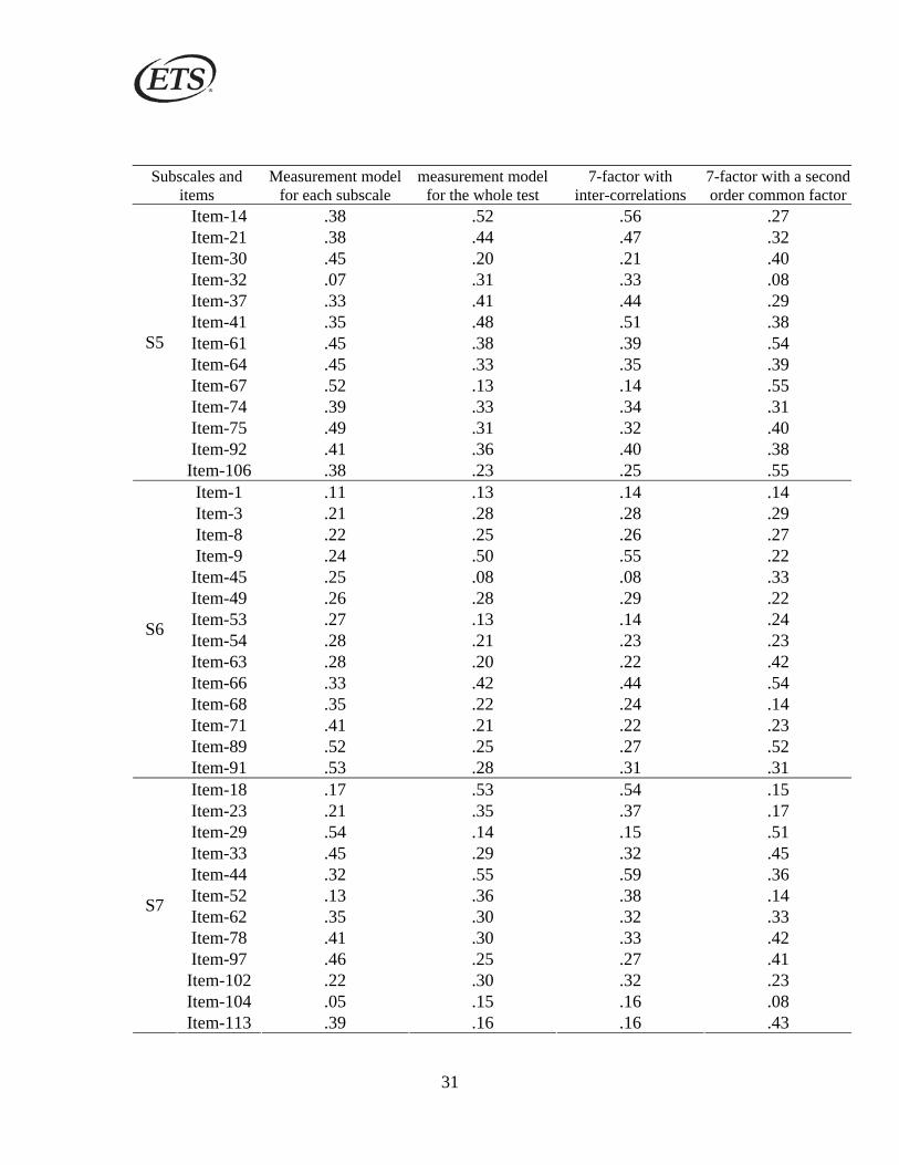
Appendix B. Item-Factor Loadings of the Item Level Factor Models

Subscales and items

Measurement model for each subscale

measurement model for the whole test

7-factor with inter-correlations

7-factor with a second order common factor

Item-4 .14 .50 .51 .14 Item-7 .46 .07 .08 .39 Item-13 .42 .26 .27 .40 Item-24 .26 .37 .40 .19 Item-28 .36 .35 .37 .40 Item-31 .54 .26 .27 .59 Item-34 .19 .27 .29 .19 Item-38 .52 .19 .20 .54 Item-42 .35 .27 .29 .37 Item-48 .34 .39 .42 .32 Item-50 .4 .26 .29 .41 Item-82 .44 .50 .54 .53 Item-83 .5 .50 .55 .52 Item-86 .19 .35 .39 .16 Item-88 .25 .22 .23 .25 Item-95 .31 .39 .42 .21 Item-99 .37 .52 .54 .42 Item-108 .26 .20 .22 .29 Item-109 .34 .48 .52 .38 Item-110 .28 .31 .56

S1

Item-115 .65 .33 .35 .33 Item-5 .35 .22 .23 .35 Item-10 .49 .23 .23 .50 Item-11 .31 .27 .29 .27 Item-15 .5 .37 .39 .53 Item-19 .28 .30 .33 .21 Item-26 .22 .51 .53 .20 Item-51 .44 .51 .54 .44 Item-55 .35 .35 .38 .33 Item-56 .24 .34 .37 .22 Item-58 .5 .33 .36 .51 Item-69 .48 .21 .23 .44 Item-81 .59 .50 .52 .54 Item-85 .51 .42 .44 .47 Item-93 .39 .60 .62 .39 Item-94 .19 .35 .38 .16 Item-96 .34 .35 .38 .35 Item-103 .19 .45 .47 .16 Item-105 .28 .25 .26 .26

S2

Item-107 .2 .48 .52 .23

30

Item-118 .17 .50 .51 .14 Subscales and

items Measurement model

for each subscale measurement model

for the whole test 7-factor with

inter-correlations 7-factor with a second order common factor

Item-16 .49 .28 .30 .50 Item-20 .32 .36 .37 .33 Item-22 .32 .16 .17 .29 Item-25 .46 .25 .28 .44 Item-27 .17 .47 .50 .14 Item-35 .42 .15 .17 .42 Item-39 .41 .13 .14 .38 Item-40 .24 .37 .40 .23 Item-46 .48 .42 .45 .47 Item-60 .38 .44 .47 .38 Item-70 .57 .32 .33 .53 Item-72 .31 .49 .51 .27 Item-77 .33 .49 .53 .38 Item-79 .4 .39 .42 .38 Item-84 .34 .13 .14 .32 Item-90 .46 .30 .31 .52 Item-111 .39 .34 .38 .39 Item-112 .27 .38 .39 .30

S3

Item-117 .41 .48 .50 .47 Item-2 .21 .48 .50 .27 Item-6 .34 .16 .16 .32 Item-12 .36 .35 .38 .37 Item-17 .4 .41 .44 .37 Item-36 .29 .17 .19 .29 Item-43 .33 .36 .40 .33 Item-47 .43 .18 .19 .39 Item-57 .48 .32 .33 .51 Item-59 .36 .30 .33 .34 Item-65 .53 .38 .41 .52 Item-73 .26 .49 .51 .31 Item-76 .62 .36 .38 .62 Item-80 .53 .35 .39 .51 Item-87 .26 .49 .53 .26 Item-98 .52 .50 .51 .50 Item-100 .26 .49 .53 .28 Item-101 .51 .48 .52 .51 Item-114 .54 .19 .21 .54

S4

Item-116 .39 .39 .41 .37

31

Subscales and items

Measurement model for each subscale

measurement model for the whole test

7-factor with inter-correlations

7-factor with a second order common factor

Item-14 .38 .52 .56 .27 Item-21 .38 .44 .47 .32 Item-30 .45 .20 .21 .40 Item-32 .07 .31 .33 .08 Item-37 .33 .41 .44 .29 Item-41 .35 .48 .51 .38 Item-61 .45 .38 .39 .54 Item-64 .45 .33 .35 .39 Item-67 .52 .13 .14 .55 Item-74 .39 .33 .34 .31 Item-75 .49 .31 .32 .40 Item-92 .41 .36 .40 .38

S5

Item-106 .38 .23 .25 .55 Item-1 .11 .13 .14 .14 Item-3 .21 .28 .28 .29 Item-8 .22 .25 .26 .27 Item-9 .24 .50 .55 .22 Item-45 .25 .08 .08 .33 Item-49 .26 .28 .29 .22 Item-53 .27 .13 .14 .24 Item-54 .28 .21 .23 .23 Item-63 .28 .20 .22 .42 Item-66 .33 .42 .44 .54 Item-68 .35 .22 .24 .14 Item-71 .41 .21 .22 .23 Item-89 .52 .25 .27 .52

S6

Item-91 .53 .28 .31 .31 Item-18 .17 .53 .54 .15 Item-23 .21 .35 .37 .17 Item-29 .54 .14 .15 .51 Item-33 .45 .29 .32 .45 Item-44 .32 .55 .59 .36 Item-52 .13 .36 .38 .14 Item-62 .35 .30 .32 .33 Item-78 .41 .30 .33 .42 Item-97 .46 .25 .27 .41 Item-102 .22 .30 .32 .23 Item-104 .05 .15 .16 .08

S7

Item-113 .39 .16 .16 .43

32

Appendix C.

Conceptual Model for the MFT (Business): Single Factor Measurement Model.

Item 1

Item 2

…… f

Item 118

33

Appendix D:

Conceptual Model for the MFT (Business): Seven Subscales With Inter-

Correlations.

34

S1

Item 1

Item 21

……

S2

Item 1

Item 20

……

S3

Item 1

Item 19

……

S4

Item 1

Item 19

……

S5

Item 1

Item 13

……

S7

Item 1

Item 12

……

S6

Item 1

Item 14

……

35

Appendix E:

Conceptual Model for the MFT (Business), Seven Subscales with A Second Order

Factor.

36

S1

Item 1

Item 21

……

S2

Item 1

Item 20

……

S3

Item 1

Item 19

……

S4

Item 1

Item 19

……

S5

Item 1

Item 13

……

S7

Item 1

Item 12

……

S6

Item 1

Item 14

……

f