IZA DP No. 926

Why the Apple Doesn’t Fall Far:Understanding IntergenerationalTransmission of Human Capital

Sandra E. BlackPaul J. DevereuxKjell G. Salvanes

DI

SC

US

SI

ON

PA

PE

R S

ER

IE

S

Forschungsinstitutzur Zukunft der ArbeitInstitute for the Studyof Labor

November 2003

Why the Apple Doesn’t Fall Far: Understanding Intergenerational Transmission of Human Capital

Sandra E. Black UCLA, NBER and IZA Bonn

Paul J. Devereux

UCLA and IZA Bonn

Kjell G. Salvanes Norwegian School of Economics, Statistics Norway and IZA Bonn

Discussion Paper No. 926 November 2003

IZA

P.O. Box 7240 D-53072 Bonn

Germany

Tel.: +49-228-3894-0 Fax: +49-228-3894-210

Email: iza@iza.org

This Discussion Paper is issued within the framework of IZA’s research area The Future of Labor. Any opinions expressed here are those of the author(s) and not those of the institute. Research disseminated by IZA may include views on policy, but the institute itself takes no institutional policy positions. The Institute for the Study of Labor (IZA) in Bonn is a local and virtual international research center and a place of communication between science, politics and business. IZA is an independent, nonprofit limited liability company (Gesellschaft mit beschränkter Haftung) supported by Deutsche Post World Net. The center is associated with the University of Bonn and offers a stimulating research environment through its research networks, research support, and visitors and doctoral programs. IZA engages in (i) original and internationally competitive research in all fields of labor economics, (ii) development of policy concepts, and (iii) dissemination of research results and concepts to the interested public. The current research program deals with (1) mobility and flexibility of labor, (2) internationalization of labor markets, (3) welfare state and labor market, (4) labor markets in transition countries, (5) the future of labor, (6) evaluation of labor market policies and projects and (7) general labor economics. IZA Discussion Papers often represent preliminary work and are circulated to encourage discussion. Citation of such a paper should account for its provisional character. A revised version may be available on the IZA website (www.iza.org) or directly from the author.

IZA Discussion Paper No. 926 November 2003

ABSTRACT

Why the Apple Doesn’t Fall Far: Understanding Intergenerational Transmission of Human Capital∗

Parents with higher education levels have children with higher education levels. However, is this because parental education actually changes the outcomes of children, suggesting an important spillover of education policies, or is it merely that more able individuals who have higher education also have more able children? This paper proposes to answer this question by using a unique dataset from Norway. Using the reform of the education system that was implemented in different municipalities at different times in the 1960s as an instrument for parental education, we find little evidence of a causal relationship between parents’ education and children’s education, despite significant OLS relationships. We find 2SLS estimates that are consistently lower than the OLS estimates with the only statistically significant effect being a positive relationship between mother's education and son's education. These findings suggest that the high correlations between parents’ and children’s education are due primarily to family characteristics and inherited ability and not education spillovers. JEL Classification: I21, J13, J24 Keywords: intergenerational mobility, education, educational reform Corresponding author: Sandra E. Black Department of Economics UCLA Box 951477 Los Angeles, CA 90095 USA Tel: +1 310 825 5665 Email: sblack@econ.ucla.edu

∗ The authors would like to thank Marina Bassi for helpful research assistance. We also thank Maia Guell, Oskar Nordstrøm Skans, and participants at ESSLE, SoLE, ITAM, the CEPR Uppsala Workshop, and at UCL for helpful suggestions.

1. Introduction

Parents with higher education levels have children with higher education levels.

But why? There are a number of possible explanations. One is a pure selection story; the

type of parent who has more education, earns higher salaries, etc, has the type of child

who will do so as well, regardless. Another story is one of causation; attaining more

education makes you a different type of parent, and thus leads to your children having

higher educational outcomes.

Distinguishing between these scenarios is important from a policy perspective.

One of the key roles of publicly provided education in our society is to increase equality

of opportunity, and many policies have been implemented to further that goal in recent

years.1 Proponents of this type of education policy often cite as one of the benefits the

spillover effects on to later generations; having more educated citizens will have longer

run effects by improving the outcomes of their children. While many argue that this is

the case, there is little causal evidence to suggest it is true; the research to date has been

limited in its ability to distinguish between selection and causation.

This paper proposes to provide evidence on the causal link between parents’ and

children’s education by using a unique dataset from Norway. During the 1960s, there

was a drastic change in the compulsory schooling laws affecting primary and middle

schools. Pre-reform, the Norwegian education system required children to attend school

through the seventh grade; after the reform, this was extended to the ninth grade, adding

two years of required schooling. Additionally, implementation of the reform occurred in

different municipalities at different times, starting in 1960 and continuing through 1972,

allowing for regional as well as time series variation. Evidence in the literature suggests

2

that these reforms had a large and significant impact on educational attainment which, in

turn, led to a significant increase in earnings.2 As a result, the reform provides variation

in parental education that is exogenous to parental ability and enables us to determine the

impact of increasing parental education on children’s schooling decisions. Although the

instrument only allows us to determine the impact of increasing parental education from

seven to nine years, this may be an important starting point for identifying the

intergenerational transmission of education.

Using this reform as an instrument for parental education, we find little evidence

of a causal relationship between father’s education and children’s education, despite

significant and large OLS relationships. We find a small but significant causal

relationship between mother’s education and her son’s education but no causal

relationship between mother’s and daughter’s educations. This suggests that high

correlations between parental and children’s education are due primarily to selection and

not causation.

The paper unfolds as follows: Sections 2 and 3 will discuss relevant literature and

describe the Norwegian Education reform. Sections 4 and 5 describe our empirical

strategy and data. Section 6 discusses the effect of the Norwegian education reform on

educational attainment, and Section 7 presents our results, providing first separate

estimates of the effects of mothers' and fathers' education and then the results when both

are included at the same time. Section 8 presents some specification checks, including

checks for sample selection problems due to the age of our sample, selection into

1 For example, the “No Child Left Behind” program supported by President George W. Bush. 2 See Aakvik, Salavanes, and Vaage, 2003. Results on the impact of similar reforms on educational attendance also exists for Sweden, see Meghir and Palme (2003) and for England and Ireland, see Harmon and Walker (1995) and Oreopulos (2003).

3

parenthood, and sibling fixed effects. Finally, Section 9 attempts to disentangle some

possible explanations for the positive causal relationship we observe between education

of mothers and sons, first looking at marital choices and then considering whether

quality/quantity tradeoffs made by more educated women can explain the result. Section

10 then concludes.

2. Background Information

There is an extensive literature on the intergenerational transmission of income

that focuses on the correlation of parental and children’s permanent income.3 In work

comparing Scandinavian countries with the United States, the evidence suggests that the

more compressed is the income distribution, the smaller the correlation between parental

and child outcomes. Bjorklund and Jantti (1997) compare intergenerational mobility in

the U.S. and Sweden and find some evidence that intergenerational mobility is higher in

Sweden. Bjorklund et al. (2002) extend this to include a comparison of intergenerational

mobility in the U.S. to Norway, Denmark, Sweden and Finland and find support for

greater income mobility in all the Scandinavian countries than in the US. Bratberg,

Nilsen, and Vaage (2002) also explore the relationship between income inequality and

mobility, focusing specifically on Norway, and argue that, over time, the compression of

the earnings structure in Norway has increased intergenerational earnings mobility.

However, few studies focus on intergenerational mobility in education. Results

from the US and UK suggest intergenerational education elasticities between 0.20 and

0.45 (Dearden et al., 1997; Mulligan, 1999). Using brother correlations in adult

3 For a review of this literature, see Solon (1999).

4

educational attainment as an overall measure of family and neighborhood effects, Raaum,

Salvanes and Sorensen (2001) find results for Norway that are similar to those Solon

(1999) reports for the US. None of these studies, however, attempts to distinguish a

causal relationship.

In recent work, there has been some effort to distinguish causation from mere

correlation in ability across generations. Three broad approaches have been used:

identical twins, adoptees, and instrumental variables. Behrman and Rosenzweig (2002)

use data on pairs of identical twin parents to “difference out” any correlation attributable

to genetics. Simple OLS estimates, even controlling for father’s schooling and father’s

log earnings, suggest a positive and significant relationship between mother’s and

children’s schooling (with a coefficient of 0.13 on mother’s schooling and coefficient of

0.33 on father’s schooling, both significant). However, once one looks within female

monozygotic twin pairs, thereby differencing out any genetic factors that influence

children’s schooling, the coefficient on mother’s schooling turns negative and almost

significant. The analogous fixed effects exercise using male monozygotic twin pairs

gives coefficients for father's education that are about the same size as the OLS estimates.

Recent work by Antonovics and Goldberger (2003), however, calls into question these

results and suggests that the findings are quite sensitive to the coding of the data. Also, it

may be unrealistic to assume that twins differ in terms of education but not in terms of

any other characteristic or experience that may influence the education of their offspring

(see Griliches, 1979 and Bound and Solon, 1999 for demonstrations that biases using

sibling and twin fixed effects may be as big or bigger than OLS biases).

Plug (2002) uses data on adopted children to investigate the causal relationship

5

between parental education and child education. If children are randomly placed with

adoptive parents, the relationship between parental education and child education cannot

simply reflect genetic factors. Plug finds a positive effect of father's education on child

education but no significant effect for mothers. There are a number of limitations of this

approach: sample sizes are tiny, children are not randomly placed with adoptive parents,

and the correlation between parents' education and child education could be picking up

the effects of any unobserved parental characteristic (patience, ability) that influences

child outcomes.4

Closest to our paper is work by Chevalier (2003), who uses a change in the

compulsory schooling law in Britain in 1957 to identify the effect of parental education

on their offspring’s education. He finds a large positive effect of mother’s education on

her child’s education but no significant effect of paternal education. However, this paper

suffers from the fact that the legislation was implemented nationwide; as a result, there is

no cross-sectional variation in the British compulsory schooling law. Chevalier uses

cohorts of parents born between 1948 and 1967 and instruments parental education with a

dummy for whether they were affected by the law change, a linear trend reflecting year of

birth, and the interaction of year of birth with the law dummy. Thus, he assumes away the

presence of cohort effects in the second stage and the identifying variation in parental

education arises both from secular trends in education and the once-off change in the

law.5 Second, the sample only includes children who are still living at home with their

4 Sacerdote (2002) also uses adoptees to distinguish the effect of family background from genetic factors on children’s outcomes; however, the focus of his paper is primarily the general impact of family socio-economic status as opposed to the causal impact of parent’s education. 5 This may be a particular problem in this context as less-educated individuals are more likely to have children while young and so in a sample of individuals with children of a certain age, older individuals are likely to have more education. Thus, one would like to control for unrestricted age effects for parents.

6

parents and hence loses observations in a non-random fashion.6

3. The Norwegian Primary School Reform

In 1959, the Norwegian Parliament legislated a mandatory school reform. The

reform was characterized by three broad goals, as stated explicitly in several government

documents: 1) to increase the minimum level of education in society by extending the

number of compulsory years of education from 7 to 9 years, 2) to smooth the transition to

higher education, and 3) to enhance equality of opportunities both along socio-economic

and geographical dimensions. Prior to the reform, children started school at the age of

seven and finished compulsory education after seven years, i.e. at the age of fourteen.

After the initial 7 years, there were two tracks: the General Education System for the

higher ability students (which had a 3 year and a 5 year option) and the less selective

Middle School which involved between 1 and 3 years of vocational training. In the new

system, the starting age was still seven years old, but the time spent in compulsory

education was now nine years. After the nine years of compulsory schooling, the student

could either enroll in high school (which was made more accessible after the reform) or

vocational training.7 In addition, the reform standardized the curriculum and increased

access to schools, since 9 years of mandatory school was eventually made available in all

municipalities and enrollment in high school was less competitive.

The parliament mandated that all municipalities (the lowest level of local

6 In related work, Currie and Moretti (forthcoming) find a positive effect of mothers' educational attainment on children’s health outcomes in the U.S. using instrumental variables and fixed effects approaches. 7 The Norwegian school system has been slightly changed recently by the so-called “Reform97”. Children now start at the age of six and the time spent in compulsory education is ten years, of which seven are at primary school and three are at middle school.

7

administration) must have implemented the reform by 1973; as a result, although it was

started in 1960, implementation was not completed until 1972.8 This suggests that, for

more than a decade, Norwegian schools were divided into two separate systems; which

system you were in depended on the year you were born and the municipality in which

you lived. The first cohort that could have been involved in the reform was the one born

in 1947. They started school in 1954, and (i) either finished the pre-reform compulsory

school in 1961, or (ii) went to primary school from 1954 to 1960, followed by the post-

reform middle school from 1960 to 1963. The last cohort who could have gone through

the old system was born in 1958. This cohort started school in 1965 and finished

compulsory school in 1972.9

To receive funds from the government to implement the reform, municipalities

had to present a plan to a committee under the Ministry of Education. Once approved,

the costs of teachers and buildings would be provided by the national government. While

the criteria determining selection by the committee are somewhat unclear, the committee

did want to ensure that implementation was representative of the country, conditional on

having an acceptable plan. (Telhaug, 1969, Mediås, 2000). Figure 1 presents the spread

of the reform over time, focusing on the number of municipalities implementing the

reform per year.

While it is not necessary for our estimation strategy, it would be useful if the

timing of the implementation of the reform across municipalities were uncorrelated with

8 The reform had already started on a small and explorative basis in the late 1950s, but applied to a negligible number of students because only a few small municipalities, each with a small number of schools, were involved. See Lie (1974), Telhaug (1969), and Lindbekk (1992), for descriptions of the reform. 9 Similar school reforms were undertaken in many other European countries in the same period, notably Sweden, the United Kingdom and, to some extent, France and Germany (Leschinsky and Mayer, 1990).

8

general educational levels. One might worry that poorer municipalities would be among

the first to implement the reform, given the substantial state subsidies, while wealthier

municipalities would move much slower. However, work examining the determinants of

the timing of implementation finds no relationship between municipality characteristics

such as average earnings, taxable income, and educational levels, and the timing of

implementation. (See Lie 1973, 1974.) Municipalities that are located geographically

near municipalities that already implemented the reform were themselves more likely to

implement the reform; numerous interviews revealed that this was likely due to a

particularly effective county administrator. As a result, the research supports a complex

adoption process without finding support for a single important factor to explain the

implementation process. To examine this ourselves, Figures 2, 3, and 4 examine the

implementation of the reform by the average income, parental education, and size of the

municipalities; these figures suggest that there is little relationship between these factors

and the timing of the implementation of the reform.

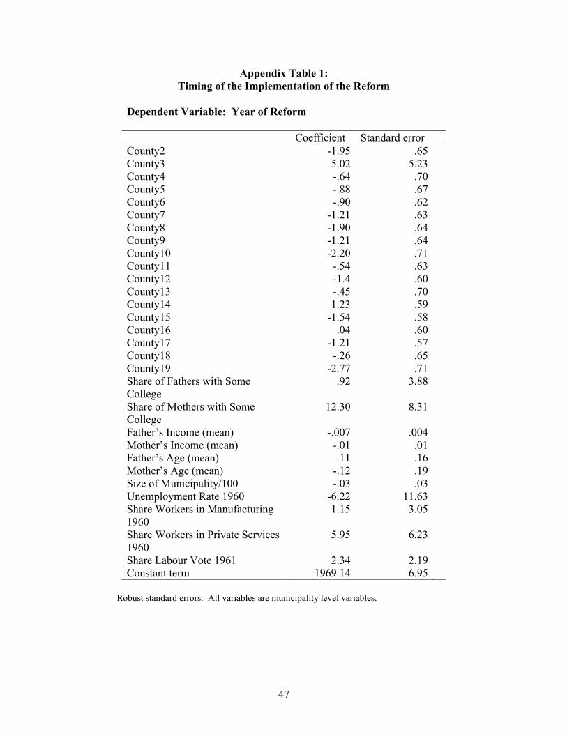
As a more rigorous test, in Appendix Table 1 we regress the year of

implementation on different background variables based on municipality averages,

including parental income, the level of education, average age, and the size of the

municipality, as well as county dummies (there are 20 counties in Norway). Consistent

with the existing literature, there appears to be no systematic relationship between the

timing of implementation and parent average earnings, education levels, average age,

urban/rural status, industry or labor force composition, municipality unemployment rates

in 1960, and the share of individuals who were members of the Labor party (the most

pro-reform and dominant political party).

9

4. Identification Strategy

To identify the causal effects of parents’ education on children’s education, it is

useful to have variation in parents’ education that is exogenous to parental ability and

other factors that are correlated with both parents’ and child’s educational choice. Our

source of exogenous variation is the education reform in Norway that increased the

number of years of compulsory schooling from 7 to 9 years and was implemented

primarily over a 12 year period from 1960 to 1971 in different municipalities at different

times. Thus, there is both time-series and cross-sectional variation in the number of years

of compulsory schooling required of individuals during this period. We then observe the

children of this generation in 2000.

Our empirical model is summarized by the following two equations:

εββββββ ++++++= Ppp TYMUNICIPALIAGEFEMALEAGEEDED 543210 (1)

υαααααα ++++++= PppP TYMUNICIPALIAGEFEMALEAGEREFORMED 543210 (2)

In equations (1) and (2), ED is the number of years of education obtained by the child,

AGE refers to a full set of years of age indicators, MUNICIPALITY refers to a full set of

municipality indicators, and REFORM equals 1 if the individual was affected by the

education reform, and 0 otherwise. In all cases, the superscript p denotes parent, so that,

for example, AGEp refers to a full set of indicator variables for the age of the parent. We

estimate the model using Two Stage Least Squares (2SLS) so that equation (2) is the first

stage and serves as an instrumental variable for . pREFORM PED

There are a few points to note about equations (1) and (2): First, both equations

contain fixed age effects and municipality effects for parents. The age effects are

10

necessary to allow for secular changes in educational attainment over time that may be

completely unrelated to the reform. For instance, at this time there was a trend in

Norway, as well as in other countries, of increasing educational attainment. The

municipality effects allow for the fact that variation in the timing of the reform across

municipalities may not have been exogenous to parents’ educational choice.10 Even if the

reform was implemented first in areas with certain unobserved characteristics, consistent

estimation is still achieved so long as (a) these characteristics are fixed over time during

the 12-year period or (b) implementation of the reform is not correlated with changes in

these characteristics or (c) these characteristics are not related to the schooling of the

children of this generation.11

Second, we have included age indicators for the children to allow for the fact that

not all children in our sample have finished schooling by 2000. Third, we do not include

any further child characteristics such as their area of residence as these are potentially

endogenous to their years of schooling. For example, suppose the reform causes a woman

to receive more education and this causes her to move to a city where educational costs

are low and, hence, her children have high education. We consider this a causal effect of

parental education on child education, even though it has arisen partly through the effect

of parental education on the residence of the child.

5. Data

10 In section 3 we argued that the available evidence suggests no systematic patterns in the timing of reform implementation across municipalities. However, for example, early adopters may differ from late adopters of the reform if they value schooling more because the industrial composition in the municipality implies greater demand for skilled workers. These types of possibilities are controlled for by municipality fixed effects. 11 In our estimation, we have also tried allowing for municipality-specific time trends as well as county by year fixed effects. Our results were insensitive to the inclusion of these extra variables.

11

Based on different administrative registers and census data from Statistics

Norway, a comprehensive data set has been compiled of the entire population in Norway,

including information on family background, age, marital status, country of birth,

educational history, neighborhood information, and employment information.12 The

initial database is linked administrative data which covers the entire population of

Norwegians aged 16-74. These administrative data provide information about

educational attainment, labor market status and a set of demographic variables (age,

gender). To this, we match extracts from the censuses in 1960, 1970 and 1980.

To determine whether parents were affected by the reform, we need to link each

parent to the municipality in which they grew up. We do this by matching the

administrative data to the 1960 census. From the 1960 census, we know the municipality

in which the parent's mother lived in 1960.13 In 1960, the parents we are using in the

estimation are aged between 2 and 13. One concern is that there may be selective

migration into or out of municipalities that implement the reform early.14 However, since

the reform implementation did not occur before 1960, this could only be a problem for us

to the extent that families anticipated where the reform would be implemented first and

made mobility decisions prior to the 1960 census. Any reform-induced mobility

subsequent to 1960 may affect the precision of our 2SLS estimates but not their

consistency.

The measure of educational attainment is taken from a separate data source

12 See Møen, Salvanes and Sørensen (2003) for a description of the data set. 13 Since very few children live with their father in the cases where parents are not living together, we should only have minimal misclassification by applying this rule. 14 Evidence from Meghir and Palme (2003) on Sweden and Telhaug (1969) on Norway suggest that reform-induced migration was not a significant consideration.

12

maintained by Statistics Norway; educational attainment is reported by the educational

establishment directly to Statistics Norway, thereby minimizing any measurement error

due to misreporting. This register provides detailed information on educational

attainment. The educational register started in 1970; for parents who completed their

education before then we use information from the 1970 Census. Thus the register data

are used for all but the earliest cohorts of parents who did not have any education after

1970. Census data are self reported (4 digit codes of types of education were reported)

and the information is considered to be very accurate; there are no spikes or changes in

the education data from the early to the later cohorts.

Our primary data source on the timing of the reform in individual municipalities

is the volume by Ness (1971). To verify the dates provided by Ness, we examined the

data to determine whether or not there appears to be a clear break in the fraction of

students with less than 9 years of education. In the rare instance when the data did not

seem consistent with the timing stated in Ness, we checked these individual

municipalities by contacting local sources.15 We are able to successfully calculate reform

indicators for 545 out of the 728 municipalities in existence in 1960. If the reform took

more than one year to implement in a particular municipality or we were not able to

verify the information given in Ness (1971), we could not assign a reform indicator to

that municipality. However, we have reform information for a large majority of

individuals in the relevant cohorts.

We include cohorts of parents born between 1947 and 1958 in our sample. The

sample of children includes all individuals in 2000 who are aged 20 - 35. Note that a

15 Between 1960 and 1970, a number of municipalities merged. In our analysis, we use the 1960 municipality as the unit of observation. In cases where the data were available at the 1970 municipality

13

great advantage of our data set over others in the literature is that we can link adult

children in 2000 to characteristics of their parents, even in cases where the children do

not live with their parents. Table 1 provides summary statistics for the individuals in our

sample.16

6. The Effects of the Reform on Educational Attainment

There is a significant literature examining the impact of compulsory schooling

laws on educational attainment.17 In Norway, the legislation mandated a full two year

change in schooling for individuals at the bottom of the educational distribution. Table 2

demonstrates the significance of this legislation. It shows the distribution of education

averaged over the 2 years prior to the reform and the two years immediately after the

reform (including the year the reform was implemented).

It is clear from this table that the primary effect of the reform was to reduce the

proportion of people with fewer than 9 years of education to almost zero. In the 2 years

prior to the change in the compulsory schooling laws, 12% of individuals completed

fewer than 9 years of schooling. After the legislative change, we see that less than 3% of

the population has fewer than 9 years of schooling, with a new spike at 9 years.18

In addition to changing the educational structure at the bottom end of the

distribution, the reform eliminated much of the tracking of students done prior to the

level, individual municipalities were contacted to determine the appropriate coding. 16 Note that it sometimes occurs that one parent is in our sample while the other is not because only one of them is born during the 1947-1958 period. 17 For work on the U.S., see, for example, Acemoglu and Angrist (1999). 18 The presence of some individuals with fewer than 9 years of schooling when the reform is in place reflects the fact that compliance with the law was not 100% and some individuals dropped out before completing compulsory schooling. It may also reflect the fact that, in some municipalities, the reform was implemented over several years and also possibly some error in the dating of reform implementation. These factors will tend to reduce the precision of our estimates without affecting consistency.

14

reform. As a result, the 3 versus 5 year General Education System was replaced by a

single high school system with more generous admission standards and availability. As a

result, the educational distribution appears to have a “hole” at 10 years of education after

the reform (See Table 2); individuals who would have done the 3 year high school track

before the reform would now have increased access to high school after 9 years of

compulsory schooling and therefore ultimately achieve 10, 11 or 12 years of schooling.

This is consistent with the fact that the proportion of individuals with 10-12 years of

education is similar before and after the reform.

Restricting the Sample

Because the primary impact of the reform is at the bottom of the educational

distribution, we conduct much of our analysis on the sample of mothers/fathers who have

9 or fewer years of education. The additional assumptions we make in doing this are 1)

that individuals who get 9 years of education after the reform would have received 9

years or less of education if the reform had not been in effect, and 2) that individuals who

got 9 years or less of education before the reform would have received 9 years of

education if the reform had been in effect.19 These are not testable but we describe below

features of the data that suggest that our assumptions are not unreasonable.

First, consider Table 2. In this table, we see that the proportion of individuals with

9 years or less of education stays constant when we compare two years before to two

years after the reform. This suggests that there may be no significant spillover effects of

the reform; those who obtained 9 or fewer years of education before the reform would

19 This second assumption rules out spillover effects of the reform of the sort that some signaling models imply.

15

have continued to do so after the reform.

Additionally, we have examined the family background characteristics of the

individuals (parents) with 9 or fewer years of education in the years before and after the

reform to check and see if the composition of our sample appears to have changed. If, for

example, there were positive spillover effects of the reform, we might expect to see the

post-reform individuals with 9 or fewer years of education looking observably “worse”

than those prior to the reform. The variables we can look at include the log of family

income and the educational attainment of the mothers and fathers (of our parents). The

log of family income comes from the 1970 census and so is less than ideal for our

purposes. However, when we regress each of these variables on the reform indicator

along with cohort and municipality effects for the sample of individuals with 9 or fewer

years of education, we find no evidence of any compositional change after the reform.

In return for making these additional assumptions and restricting the sample we

are able to estimate a much stronger first stage and more precisely estimated second stage

coefficients.20

7. Results

Because of the timing of the reform, we balance the benefits of restricting our

sample to older children (who are more likely to have completed their education by 2000)

against the cost in terms of losing more children whose parents were directly affected by

the reform. Our primary analysis will use the sample of children who were 20-35 in

2000, but we will also try restricting our sample to 25-35 year olds as a robustness check.

20 We have also tried using characteristics of the parents of our parents to split the sample based on predicted parental education rather than actual parental education. This approach gave us estimates that are

16

We will place some emphasis on whether individuals have completed 12 years of

education, as, by age 20, the vast majority of individuals who will accumulate 12 years

will have already done so. Note also that we are conditioning on age of child in the

analysis.

Results for the Full Sample

The OLS results for equation (1) are presented in Table 3, Columns 1 and 3. They

show, as expected, a positive relationship between the years of education of the parents

and their child’s education, whether the latter is measured in terms of years of education

or an indicator equal to one if the child completed at least twelve years of education (the

equivalent of a high school diploma).21 This is true, regardless of whether we match

mothers to sons, mothers to daughters, fathers to sons, or fathers to daughters. Our

estimates suggest that increasing a parent’s education by a year increases the child’s

education by about 0.15 of a year. While the sample size varies, particularly between the

father and mother regressions (due to our inability to match fathers who were not living

with the family at the time of the 1960 census), our estimates are quite similar across

samples.

Columns 2 and 4 then present our 2SLS results, where the instrument is the

indicator for whether or not the father/mother was affected by the school reform in

Norway. The 2SLS results are imprecisely estimated and are all statistically insignificant.

The standard errors are sufficiently large that the 2SLS estimates are quite uninformative:

consistent with the ones we report but were very imprecisely estimated. 21 In both the OLS and 2SLS analysis we report robust standard errors that allow for clustering at the parent's municipality-parent's cohort level. To deal with possible concerns about the effects of serial correlation on the standard errors, we have also experimented with clustering by parent's municipality and

17

one cannot rule out small or zero effects, and one also cannot generally rule out effects

that are as large or larger than OLS. The main reason for the lack of precision is the weak

first stage relationship between the reform and years of education of the father/mother:

the t-statistics for the reform indicator in the first stage are about 5. (See Table 3a for the

first stage estimates.) These relatively small t-statistics result from the fact that, while the

reform has a large effect on the educational distribution for individuals with 9 years and

less of education, it has very minor effects at higher education levels. It is clear that to

effectively use the reform as a source of exogenous variation, one needs to focus on the

very bottom tail of the education distribution, where the reform has bite.

Results for the Restricted Sample

The OLS estimates for the sample of parents with 9 or fewer years of education

are in Columns 1 and 3 of Table 4. These are reasonably similar in magnitude to the OLS

estimates for the full sample but tend to be a little higher.22 The first stage estimates are in

Table 4a. Consistent with the evidence presented earlier, the first stage for the low

education sample is much stronger than is the case for the full sample. The 2SLS

estimates (Columns 2 and 4) are, as expected, much more precisely estimated than in the

full sample. They are also universally smaller than the OLS estimates. This is particularly

true for fathers: the estimates are all close to zero and statistically insignificant. For

found the 2SLS standard errors to be almost identical. 22 The OLS estimates may be slightly higher because, when we select individuals with less educated parents, the children are more likely to have finished their education by age 20. An offsetting factor is that, in this sample, the OLS estimates are more similar to the 2SLS estimates than would be the case from a conventional cross-sectional OLS regression. This is because individuals with 9 years of education post-reform may have chosen fewer years of education in the absence of the reform. Hence, the positive correlation between education and unobserved ability that would tend to bias the OLS coefficients upwards is reduced by the presence of the reform. Indeed when we carry out OLS regression using only pre-reform observations, we find larger OLS coefficient values.

18

mothers, the evidence suggests a positive effect of maternal education on the education of

sons but no such relationship for daughters. Even the statistically significant mother/son

coefficients are smaller than the OLS coefficients. Taken as a whole, the results indicate

that the positive correlation between parent's and children's education largely represents

positive relationships between other factors that are correlated with education. These

could be ability, family background, income or other factors. The true causal effect of

parental education on child education appears to be weak.

Our finding that the IV estimates are smaller than the OLS estimates makes sense

because we expect education choice to be positively correlated with unobserved ability.

However, this finding is not in keeping with much of the returns to education literature.

Typically, IV estimates are found to be larger than OLS estimates. We suspect a few

reasons for this divergence. First, our education data is of very high quality and probably

has little or no measurement error. This is in contrast to the self-reported education data

used in most studies. Thus, unlike in other studies, our OLS estimates may not be subject

to downward biases due to measurement error. Second, our use of an education reform

and our ability to control for both age and municipality effects leads to greater confidence

that the instrument is not correlated with unobserved ability and hence our IV estimates

are not upward biased. Finally, high IV estimates in the endogenous education literature

are often rationalized by heterogeneous returns to education with particularly high returns

for the group of people whose behavior is impacted by the instrument being used.

Because credit constraints are unlikely to have been a major determinant of educational

choice in the lower tail of the Norwegian distribution at this time, it is plausible that the

returns to education for individuals impacted by the reform are no higher than the

19

average.23

The Education of Both Parents

So far, we have looked at the effects of mother's and father's education separately.

These estimates take account of all ways in which one parent's education affects the

child’s education, including the effects of assortative mating -- that is, mother's education

may affect child education both directly and also indirectly because highly educated

mothers tend to marry more educated fathers. In this section, we include both mother's

and father's education in the same specification. As such, we can separate out the direct

effects of each parent's education from the indirect effects coming through assortative

mating (which we will examine directly later in the paper). Because both mother's and

father's education are endogenous, we need instruments for each of them. These are

available to us because, since many individuals are of a different age or grew up in a

different municipality than their spouse, the reform variable is potentially different for

each spouse. For example, the husband may have gone to school pre-reform, but his

younger wife may have been impacted by the reform.

When including both parents’ education in the specification, the weak first stage

when the full education distribution is used is an even greater problem than before. When

we use the full sample, the estimates of both education variables are extremely imprecise.

Once again, we need to make use of the fact that the reform only changed the education

distribution in the lower tail. To do so, we use a sample of parental pairs such that at least

23 Note that one might be concerned that the children of low-education parents will always get the minimum education mandated by law and, as a result, we will see all the children of the low-education parents clustered around 9 years of education. However, in fact this is not the case; only about 9% of the children’s generation does the minimum of 9 years of education.

20

one of the two parents had fewer than 10 years of schooling. This allows us to keep all

individuals with fewer than 10 years of schooling in the sample and also to keep their

spouses. We make one further change to the sample used earlier: Because mothers and

fathers tend to differ in age, we do not restrict the sample to the reform cohorts but

instead include any couple in which at least one of the two parents is in the reform

cohorts. Thus, we do not exclude couples just because one of them was born outside of

the reform cohorts.

Our results are presented in Table 5.24 While our results are less precise, they are

consistent with the results obtained in our earlier, separate regressions. OLS estimates

suggest a positive relationship between parents’ education and that of the children, with

estimates for mother’s education slightly larger than those for father’s education.

However, IV estimates using the Norwegian school reform find no relationship between

father’s education and his children’s education. (First stage results are presented in Table

5a.) We find some impact of mother’s education on her children’s education, although

these estimates become statistically insignificant when we break the sample down into

sons and daughters.

8. Robustness/Specification Checks

We have carried out numerous specification checks. As mentioned earlier, we

have tried adding municipality-specific time trends and county-cohort fixed effects. To

allow for possible mismeasurement of the exact timing of reform implementation, we

have also tried dropping the reform year, and dropping the reform year and the years

24 Note that, similar to earlier specifications, we also include indicators for father’s age, mother’s age, father’s municipality, mother’s municipality, and child’s age.

21

immediately preceding and following it. None of these changes affected the results.

Below we describe some more substantial specification checks.

Specification Check: Sample Selection

Given the population of data available from Statistics Norway, we were able to

avoid many potential problems of sample selection. One selection criterion we do apply

is to use children who are between 20-35 years old in 2000. One concern is that, by

doing this, we may be including children who have not yet completed their education at

the time of the survey. Given that our instrument is most effective for the lower end of

the educational distribution (and less educated parents tend to have less educated

children), it is unlikely that we are biasing our results much by including the younger

children. However, as a sensitivity check, we estimate the relationship between parents’

and children’s education on a subsample of 25-35 year olds whose parents have fewer

than 10 years of education. These results are presented in Tables 6 and 6a. Consistent

with our earlier results, we find the same positive and significant relationship for mothers

and sons but no evidence of a relationship for mothers and daughters or fathers and sons

or daughters.

Specification Check: Highly Educated

The Norwegian education reform increased compulsory schooling from 7 to 9

years. As a result, we should see little effect of the reform on the educational attainment

of more highly educated individuals. To verify this, we estimated our first and second

stages on a subsample of individuals whose parents had completed at least 12 years of

22

education. These results are presented in Tables 7 and 7a. As expected, the first stage

has no predictive power and the IV results are meaningless.

Specification Check: Selection into Parenthood

Another potential concern is the selection of individuals into parenthood. For

example, suppose women with low human capital are more likely to become mothers,

and this also varies by ability. That is, conditional on human capital, high ability women

are less likely to have children. If the reform raises the human capital of a subgroup of

women, then the high ability women in that subgroup may now choose not to have

children. This would imply that the average ability level of mothers subject to the reform

is lower than the average ability of mothers not subject to the reform. Hence, our IV

results would be biased towards zero. One check on this possibility is to examine whether

the reform affects the probability that an individual becomes a parent. If the reform has

no impact on this probability, then it is unlikely to affect the sorting into parenthood by

ability level.

Table 8 presents the results when we estimate a linear probability model on the

sample of all individuals born between 1947-1958, with the dependent variable equal to

one if the individual has one or more children in our sample of 20-35 year olds. Our

variable of interest is the reform indicator. As always, we include municipality and cohort

indicators in the specification. The results suggest that there is no relationship between

the reform and the likelihood an individual has a child in our sample; the estimated

coefficients are both economically small and statistically insignificant.

23

Sibling Fixed Effects

The use of sibling fixed effects is common in the literature. While we are not

convinced by the argument that education is exogenous conditional on these fixed effects,

we consider it a useful exercise to see how inclusion of these controls affects the OLS

results. If parent's education is positively related to unobserved ability, we would expect

that inclusion of sibling fixed effects would reduce the OLS coefficients. Although there

is no specific family identifier in our data, we can identify siblings as individuals with

identical parents.

Table 9 presents the results when we estimate the relationship between parents’

and children’s education on same-sex sibling pairs of parents (Note that both siblings

must have children in our sample to be included.) In this case, we are comparing

differences in the educational attainment of brother or sister pairs and relating that

difference to the difference in educational attainment of their children.25 Despite this

seemingly restrictive sample selection, our sample sizes were still quite large, with at

least 40,000 of each parent-child sex pairing. The OLS estimates are quite similar to

those estimated on our full sample, and the fixed effects estimates are uniformly lower

than the OLS estimates. Given that measurement error is not a major problem with our

education data, we interpret these findings as suggesting that the OLS estimates are

biased upwards because more able children or children with better family background are

more likely to obtain more schooling. We don't put much faith in the siblings fixed

effects estimates themselves because siblings with different levels of education are likely

25 Note that we also tried using sibling pairs and instrumenting for the parent’s education using the educational reform. In this case, we are relating differences in educational attainment of two brothers or sisters induced by the reform to differences in educational attainment of their children. Unfortunately, our results were too imprecise to draw any conclusions.

24

to have different ability levels. However, we see the estimates as providing more

evidence that the true causal effect of parental education is lower than suggested by OLS

estimates.

9. Interpretation of the Results

In the previous section, we found no evidence of a causal effect of father's

education on child education but some evidence that mother's education affects the

education of sons. Although theory provides very little guidance on this, we consider it

plausible that mothers' education may matter more than fathers', given that children tend

to spend much more time with their mother. It is more difficult to explain why mother's

education may be more important to their sons than their daughters.26 In this section, we

explore the mechanisms through which mothers' education may affect her child’s

education. The tone here is speculative, as there are many possible mechanisms and we

have limited information with which to disentangle them.

The most direct mechanism is that extra schooling increases human capital of the

mother and directly increases the optimal human capital choice of children. This could

arise because the return to human capital is higher for individuals who have more

educated parents or because the costs of human capital accumulation are lower (maybe

because their parents can help them more with their schoolwork). While this direct

mechanism is plausible, there are many alternative routes by which mothers' human

capital can transmit into greater child education.

26 Interestingly, Chevalier (2003) also finds this result using British data. Furthermore, Fernandez et al. (2002) provide evidence that men's decisions in the marriage market are strongly influenced by the

25

The Man You Marry

One possibility is that more educated women marry men who have more

education, higher income, and greater ability than the men married by less educated

women. If so, increasing a woman's education level may lead her children to have more

education because of genetic transmission of traits from the chosen husband.27 Even in

the absence of the genetic transmission, the husband's characteristics may impact the

child's choice of schooling level. While we know that, in general, more educated women

marry men with higher education and income levels, we now check whether this factor is

driving our 2SLS results. To do so, we regress father's education and earnings on

mother's education using the reform as instrument for mother's education. These results

are presented in Table 10. We find the 2SLS estimates of the effects of mother’s

education on father’s education and log earnings to be small and statistically insignificant

for both the full sample and the sample of mothers with education of less than 10 years.28

In contrast, as expected, the OLS estimates are significantly positive in each case.

The above evidence suggests that greater education induced by the reform did not

have any major effect on the type of father chosen by the mother. This does not

necessarily imply that it is mother's human capital per se that influences the child.

Women with higher education have higher earnings, have higher labor market

participation rates, and live in nicer neighborhoods. Unfortunately, given we only have

one instrument, we cannot distinguish whether it is the additional human capital of the

characteristics of their mothers. 27 It would be difficult to square this kind of genetic explanation with the fact that we find mothers influence boy's behavior but not girls. 28 This occurs despite the fact that women are likely to marry men who may also have the same reform experience because they are similar in age and from the same area. This factor should trivially make it more likely we find positive 2SLS relationships between husband's and wife's education.

26

mother itself or other factors that education gives rise to that matter.

Quality/Quantity Tradeoff

Yet another mechanism that could be at work is that women with more education

may choose to have fewer children and to invest more in each one of them. We examine

this mechanism by looking at the impact of mother’s education on the total number of

children each mother has. To do so, we regress the total number of children on mother’s

education using the reform as an instrument for mother’s education. These results are

presented in Table 11.29 We present the results for the whole sample and then for the

sample of mothers with fewer than 10 years of education, where our instrument has the

most impact. The OLS results for the full sample (but not the low education sample)

suggest that there is no effect of mother’s education on the number of children she has,

and the 2SLS results for both samples confirm this result. We therefore find no evidence

of a tradeoff between quantity and quality of children as mothers acquire more education

as a result of the reform.

10. Conclusions

We know that parents who are highly educated have children who, in turn, are

highly educated. But how much of this is genetic? And how much is the direct effect of

parental education on children’s education choices? Understanding the causal effect of

education on the educational decisions of later generations can provide a crucial piece of

the puzzle in terms of understanding educational spillovers.

However, until now, we have been limited in our ability to determine the causal

27

effect of parents’ education on future generations. By applying the apparently random

increase in educational attainment of some individuals due to a large change in

compulsory schooling legislation in the 1960s and early 1970s in Norway to a unique

dataset containing the entire population of the country, we are able to estimate the causal

relationship between parents’ education and that of their children.

Despite strong OLS relationships, we find little causal relationship between

parent education and child education. The one exception is among mothers and sons;

when mothers increase their educational attainment, their sons will get more education as

well. These results are robust to a number of specification checks. In addition, we

examined some of the possible mechanisms through which this relationship may be

working, including whether the women who received more education due to the reform

married better educated or wealthier men (they don’t) and whether these more highly

educated women are making a quantity/quality tradeoff (they aren’t). While we are able

to rule out a few mechanisms, a number remain, including the most direct, which

suggests that higher education may reduce the cost (in terms of effort) of education for

the child.

Despite this, these results suggest that intergenerational spillovers may not be a

compelling argument for subsidizing education. However, it is important to remember

that we are studying an education reform that increased education at the bottom tail of the

distribution. It is plausible that a policy change that increased enrollment in higher

education would have been transmitted more successfully across generations. While

these results are compelling, much more work needs to be done on this important topic.

29 Regressions also include age and municipality indicators.

28

References Aakvik, Arild, Kjell G. Salvanes, and Kjell Vaage. 2003. “Measuring the Heterogeneity

in the Returns to Education in Norway Using Educational Reforms.” CEPR DP 4088.

Acemoglu, Daron and Joshua Angrist. 1999. “How Large Are the Social Returns to

Education? Evidence from Compulsory Schooling Laws.” NBER Working Paper 7444.

Antonovics, Kate L. and Arthur S. Goldberger. 2003. “Do Educated Women Make Bad

Mothers? Twin Studies and the Intergenerational Transmission of Human Capital.” Mimeo.

Bjørklund, Anders and Markus Jantti. 1997. “Intergenerational Income Mobility in

Sweden Compared to the United States.” American Economic Review, 87(5), pp 1009-1018.

Björklund, Anders, Tor Eriksson, Markus Jännti, Oddbjørn Raaum and Erik Österbacka.

2002. “Brother correlations in earnings in Denmark, Finland, Norway and Sweden compared to the United States.” Journal of Population Economics

Bratberg, Espen, Øivind Anti Nilsen, and Kjell Vaage. 2002. “Assessing Changes in

Intergenerational Earnings Mobility.” Centre for Economic Studies in Social Insurance Working Paper No. 54, University of Bergen, December.

Behrman, Jere R. and Mark R. Rosenzweig. 2002. “Does Increasing Women’s

Schooling Raise the Schooling of the Next Generation?” American Economic Review, 91(1), pp 323-334.

Bound, John and Gary Solon. 1999. "Double Trouble: On the Value of Twins-Based

Estimation of the Returns to Schooling." Economics of Education Review, 18, pp 169-182.

Currie, Janet and Enrico Morietti. 2003. “Mother's Education and the Intergenerational

Transmission of Human Capital: Evidence from College Openings." Quarterly Journal of Economics, forthcoming.

Chevalier, Arnaud. 2003. “Parental Education and Child’s Education: A Natural

Experiment.” Mimeo, University College Dublin. Dearden, L, S. Machin and H. Reed. 1997. “Intergenerational Mobility in Britain.”

Economic Journal, 107, 47-66. Fernandez , Raquel, Alessandra Fogli, and Claudia Olivetti. 2002. "Marrying Your Mom:

29

Preference Transmission and Women's Labor and Education Choices" NBER Working Paper #9234.

Griliches, Zvi. 1979. "Sibling Models and Data in Economics: Beginnings of a Survey."

Journal of Political Economy, 87, pp 37-64. Harmon, C. and Ian Walker. 1995. “Estimates of the Economic Return to Schooling for

the United Kingdom.” American Economic Review, 85, 1278-86. Leschinsky, A. and Mayer, K. A. (eds.) (1990). The Comprehensive School Experiment

Revisited: Evidence from Western Europe. Frankfurt am Main. Lie, Suzanne S. (1973) The Norwegian Comprehensive School Reform. Strategies for

Implementation and Complying with Regulated Social Change. A Diffusion Study. Part 1 and II. Washington, D.C., The American University.

Lie, Suzanne S. (1974) ”Regulated Social Change: a Diffusion Study of the Norwegian

Comprehensive School Reform”, Acta Sociologica, 16(4), 332-350. Lindbekk, Tore (1992) ``School Reforms in Norway and Sweden and the Redistribution

of Educational Attainment.'' Journal of Educational Research, 37(2), 129-49. Mediås, Olav A. (2000). Fra griffel til PC. In Norwegian. (From pencil to PC). Steinkjer:

Steinkjer kommune. Meghir, Costas and Marten Palme. 2003. “Ability, parenthal background and education

policy: empirical evidence from a social experiment”, mimeo, Stockholm School of Economics.

Mulligan, C. 1999. “Galton versus the human capital approach to inheritance.” Journal of

Political Economy, 107, 184-224. Møen, Jarle, Kjell G. Salvanes and Erik Ø. Sørensen. 2003. “Documentation of the

Linked Empoyer-Employee Data Base at the Norwegian School of Economics.” Mimeo, The Norwegian School of Economics and Business Administration.

Ness, Erik (ed.). (1971). Skolens Årbok 1971. In Norwegian. (The primary school

yearbook 1971.) Oslo: Johan Grundt Tanum Forlag. Oreopoulos, P. 2003. “Do dropouts drop out too soon?” Mimeo, University of Toronto,. Plug, Erik. 2002. "How do Parents Raise the Educational Attainment of Future

Generations?", IZA Discussion Paper No. 652. Raaum, O., Salvanes, K.G. and Sørensen, E. Ø. (2001). ”The Neighbourhood is not what

it used to be. Discussion paper 36/2001, The Norwegian School of Economics and

30

Business Administration. Raaum, Oddbjørn, Kjell G. Salvanes, Erik Ø. Sørensen (2003) “The Impact of a Primary

School Reform on Social stratification: A Norwegian study of Neighbour and School Mate Correlations.'' The Swedish Journal of Economic Policy, 8(2).

Sacerdote, Bruce (2002). “The Nature and Nurture of Economic Outcomes.” American Economic Review, 92(2), pp 344-348. Solon, Gary (1999). “Intergenerational Mobility in the Labor Market.” In Handbook of

Labor Economics, Volume 3. O. Ashenfelter and D. Card, editors. pp 1761-1800.

Telhaug, Arne O. (1969). Den 9-årige skolen og differensieringsproblemet. En oversikt

over den historiske utvikling og den aktuelle debatt. In Norwegian. (The 9-years compulsory school and the tracking problem. An overview of the historical development and the current debate). Oslo: Lærerstudentenes Forlag.

31

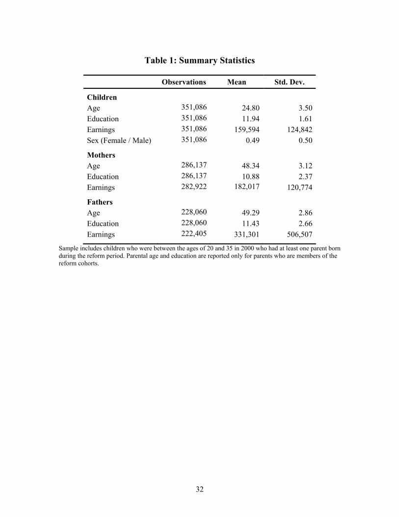
Table 1: Summary Statistics

Observations Mean Std. Dev.

Children Age 351,086 24.80 3.50 Education 351,086 11.94 1.61 Earnings 351,086 159,594 124,842 Sex (Female / Male) 351,086 0.49 0.50

Mothers Age 286,137 48.34 3.12 Education 286,137 10.88 2.37 Earnings 282,922 182,017 120,774

Fathers Age 228,060 49.29 2.86 Education 228,060 11.43 2.66 Earnings 222,405 331,301 506,507

Sample includes children who were between the ages of 20 and 35 in 2000 who had at least one parent born during the reform period. Parental age and education are reported only for parents who are members of the reform cohorts.

32

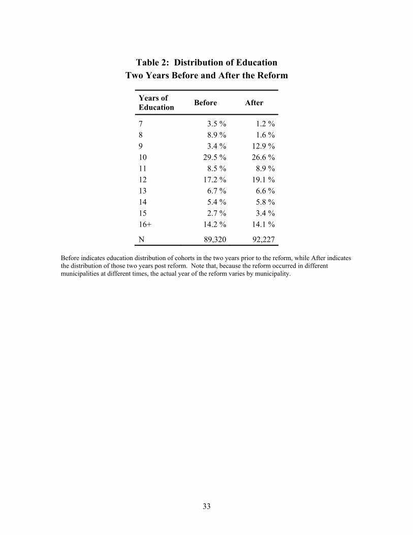
Table 2: Distribution of Education Two Years Before and After the Reform

Years of Education Before After

7 3.5 % 1.2 %8 8.9 % 1.6 %9 3.4 % 12.9 %10 29.5 % 26.6 %11 8.5 % 8.9 %12 17.2 % 19.1 %13 6.7 % 6.6 %14 5.4 % 5.8 %15 2.7 % 3.4 %16+ 14.2 % 14.1 %

N 89,320 92,227

Before indicates education distribution of cohorts in the two years prior to the reform, while After indicates the distribution of those two years post reform. Note that, because the reform occurred in different municipalities at different times, the actual year of the reform varies by municipality.

33

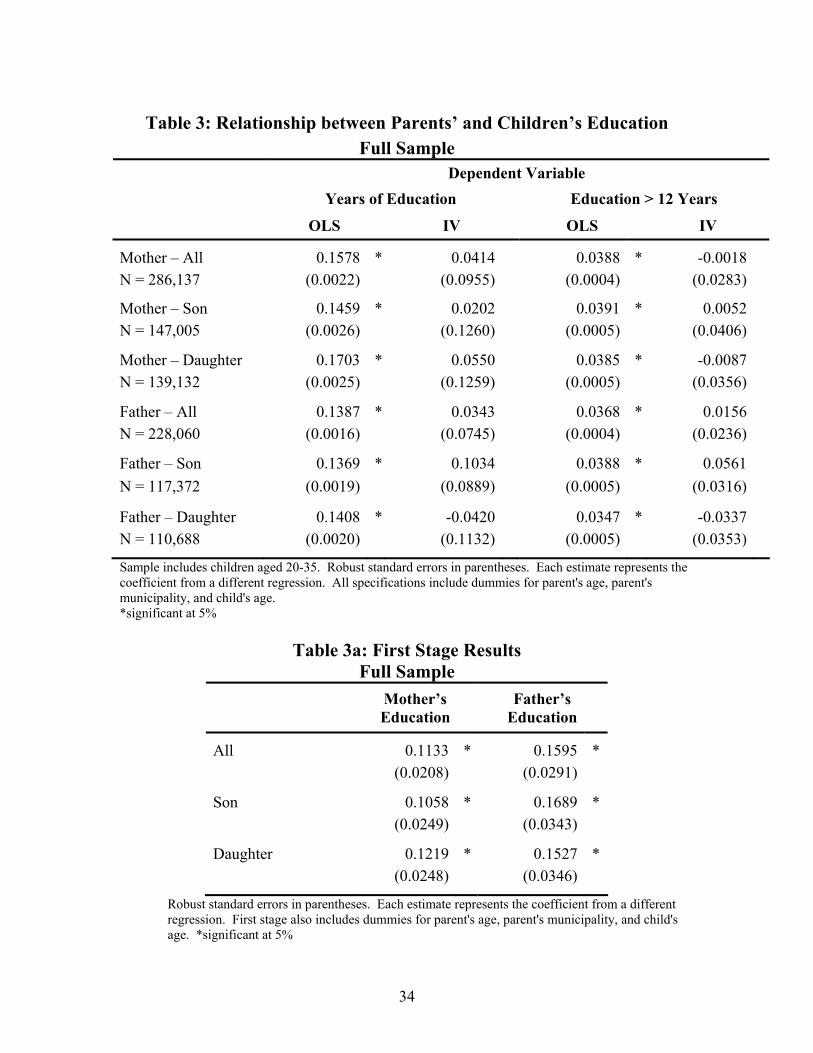
Table 3: Relationship between Parents’ and Children’s Education Full Sample

Dependent Variable Years of Education Education > 12 Years

OLS IV OLS IV

Mother – All 0.1578 * 0.0414 0.0388 * -0.0018 N = 286,137 (0.0022) (0.0955) (0.0004) (0.0283)

Mother – Son 0.1459 * 0.0202 0.0391 * 0.0052 N = 147,005 (0.0026) (0.1260) (0.0005) (0.0406)

Mother – Daughter 0.1703 * 0.0550 0.0385 * -0.0087 N = 139,132 (0.0025) (0.1259) (0.0005) (0.0356)

Father – All 0.1387 * 0.0343 0.0368 * 0.0156 N = 228,060 (0.0016) (0.0745) (0.0004) (0.0236)

Father – Son 0.1369 * 0.1034 0.0388 * 0.0561 N = 117,372 (0.0019) (0.0889) (0.0005) (0.0316)

Father – Daughter 0.1408 * -0.0420 0.0347 * -0.0337 N = 110,688 (0.0020) (0.1132) (0.0005) (0.0353)

Sample includes children aged 20-35. Robust standard errors in parentheses. Each estimate represents the coefficient from a different regression. All specifications include dummies for parent's age, parent's municipality, and child's age. *significant at 5%

Table 3a: First Stage Results

Full Sample

Mother’s Education

Father’s Education

All 0.1133 * 0.1595 * (0.0208) (0.0291)

Son 0.1058 * 0.1689 * (0.0249) (0.0343)

Daughter 0.1219 * 0.1527 * (0.0248) (0.0346)

Robust standard errors in parentheses. Each estimate represents the coefficient from a different regression. First stage also includes dummies for parent's age, parent's municipality, and child's age. *significant at 5%

34

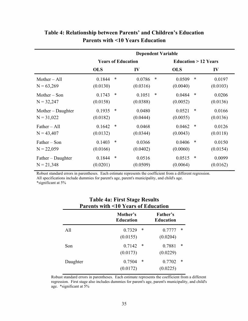
Table 4: Relationship between Parents’ and Children’s Education Parents with <10 Years Education

Dependent Variable

Years of Education Education > 12 Years

OLS IV OLS IV

Mother – All 0.1844 * 0.0786 * 0.0509 * 0.0197 N = 63,269 (0.0130) (0.0316) (0.0040) (0.0103)

Mother – Son 0.1743 * 0.1051 * 0.0484 * 0.0206 N = 32,247 (0.0158) (0.0388) (0.0052) (0.0136)

Mother – Daughter 0.1935 * 0.0480 0.0521 * 0.0166 N = 31,022 (0.0182) (0.0444) (0.0055) (0.0136)

Father – All 0.1642 * 0.0468 0.0462 * 0.0126 N = 43,407 (0.0132) (0.0344) (0.0043) (0.0118)

Father – Son 0.1403 * 0.0366 0.0406 * 0.0150 N = 22,059 (0.0166) (0.0402) (0.0060) (0.0154)

Father – Daughter 0.1844 * 0.0516 0.0515 * 0.0099 N = 21,348 (0.0201) (0.0509) (0.0064) (0.0162)

Robust standard errors in parentheses. Each estimate represents the coefficient from a different regression. All specifications include dummies for parent's age, parent's municipality, and child's age. *significant at 5%

Table 4a: First Stage Results Parents with <10 Years of Education

Mother’s Education

Father’s Education

All 0.7329 * 0.7777 * (0.0155) (0.0204)

Son 0.7142 * 0.7881 * (0.0173) (0.0229)

Daughter 0.7504 * 0.7702 * (0.0172) (0.0225)

Robust standard errors in parentheses. Each estimate represents the coefficient from a different regression. First stage also includes dummies for parent's age, parent's municipality, and child's age. *significant at 5%

35

Table 5: Relationship between Parents’ and Children’s Education Including Both Parents’ Education

If Either Parent Has <10 Years Education

Dependent Variable: Years of Education

All Children

Sons

Daughters

OLS IV OLS IV OLS IV Mother’ Education

.15* (.004)

.16* (.06)

.13* (.005)

.28 (.50)

.18* (.01)

.13 (.08)

Father’s Education .11*

(.003) -.01 (.07)

.11* (.004)

-.07 (.39)

.12* (.01)

-.03 (.09)

N 76,649 39,150 37,499

Each column represents a separate regression. Regressions also include indicators for mother’s age, father’s age, mother’s municipality, father’s municipality, and child’s age. Robust standard errors in parentheses. Sample includes children 20-35 years of age who had at least one parent born in the reform cohorts. * significant at 5% level.

Table 5a: First Stage Results If Either Parent Has <10 Years Education

All Children

Sons

Daughters Mother's

Education Father's

Education Mother's

Education Father's

Education Mother's

Education Father's

Education Mother Reform = 1 0.3876* -0.0495* 0.3636* -0.0477 0.4191* -0.0593* (0.0202)

(0.0198) (0.0286) (0.0279) (0.0288) (0.0287)

Father Reform = 1 0.0423* 0.3347* 0.0450 0.3097* 0.0419 0.3558* (0.0170)

(0.0256) (0.0240) (0.0359) (0.0245) (0.0373)

N 76,649 39,150 37,499 Each column represents one regression. Note that there are two first stage regressions, one for each parents’ education; each first stage regression included an indicator for whether the mother was affected by the reform and an indicator for whether the father was affected by the reform. Regressions also include indicators for mother’s age, father’s age, mother’s municipality, father’s municipality, and child’s age. Robust standard errors in parentheses. Sample includes children 20-35 years of age who had at least one parent born in the reform cohorts. * significant at 5% level.

36

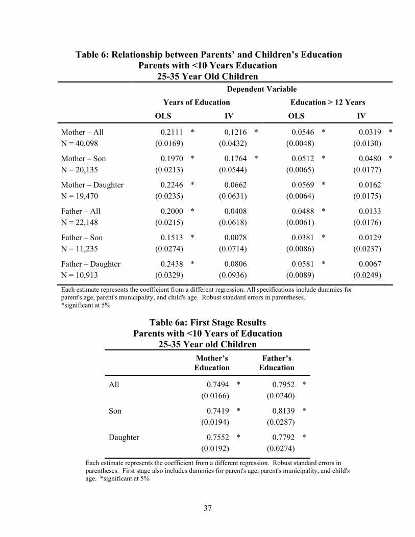
Table 6: Relationship between Parents’ and Children’s Education Parents with <10 Years Education

25-35 Year Old Children Dependent Variable

Years of Education Education > 12 Years

OLS IV OLS IV

Mother – All 0.2111 * 0.1216 * 0.0546 * 0.0319 *N = 40,098 (0.0169) (0.0432) (0.0048) (0.0130)

Mother – Son 0.1970 * 0.1764 * 0.0512 * 0.0480 *N = 20,135 (0.0213) (0.0544) (0.0065) (0.0177)

Mother – Daughter 0.2246 * 0.0662 0.0569 * 0.0162 N = 19,470 (0.0235) (0.0631) (0.0064) (0.0175)

Father – All 0.2000 * 0.0408 0.0488 * 0.0133 N = 22,148 (0.0215) (0.0618) (0.0061) (0.0176)

Father – Son 0.1513 * 0.0078 0.0381 * 0.0129 N = 11,235 (0.0274) (0.0714) (0.0086) (0.0237)

Father – Daughter 0.2438 * 0.0806 0.0581 * 0.0067 N = 10,913 (0.0329) (0.0936) (0.0089) (0.0249)

Each estimate represents the coefficient from a different regression. All specifications include dummies for parent's age, parent's municipality, and child's age. Robust standard errors in parentheses. *significant at 5%

Table 6a: First Stage Results Parents with <10 Years of Education

25-35 Year old Children

Mother’s Education

Father’s Education

All 0.7494 * 0.7952 * (0.0166) (0.0240)

Son 0.7419 * 0.8139 * (0.0194) (0.0287)

Daughter 0.7552 * 0.7792 * (0.0192) (0.0274)

Each estimate represents the coefficient from a different regression. Robust standard errors in parentheses. First stage also includes dummies for parent's age, parent's municipality, and child's age. *significant at 5%

37

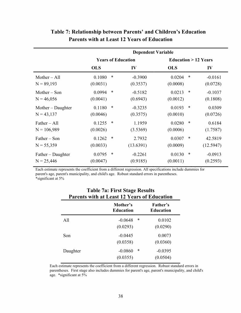
Table 7: Relationship between Parents’ and Children’s Education Parents with at Least 12 Years of Education

Dependent Variable

Years of Education Education > 12 Years

OLS IV OLS IV

Mother – All 0.1080 * -0.3900 0.0204 * -0.0161 N = 89,193 (0.0031) (0.3537) (0.0008) (0.0728)

Mother – Son 0.0994 * -0.5182 0.0213 * -0.1037 N = 46,056 (0.0041) (0.6943) (0.0012) (0.1808)

Mother – Daughter 0.1180 * -0.3235 0.0193 * 0.0309 N = 43,137 (0.0046) (0.3575) (0.0010) (0.0726)

Father – All 0.1255 * 1.1959 0.0280 * 0.6184 N = 106,989 (0.0026) (3.5369) (0.0006) (1.7587)

Father – Son 0.1262 * 2.7932 0.0307 * 42.5819 N = 55,359 (0.0033) (13.6391) (0.0009) (12.5947)

Father – Daughter 0.0795 * -0.2261 0.0130 * -0.0913 N = 25,446 (0.0047) (0.9185) (0.0011) (0.2593)

Each estimate represents the coefficient from a different regression. All specifications include dummies for parent's age, parent's municipality, and child's age. Robust standard errors in parentheses. *significant at 5%

Table 7a: First Stage Results Parents with at Least 12 Years of Education

Mother’s Education

Father’s Education

All -0.0648 * 0.0102 (0.0293) (0.0290)

Son -0.0445 0.0073 (0.0358) (0.0360)

Daughter -0.0860 * -0.0395 (0.0355) (0.0504)

Each estimate represents the coefficient from a different regression. Robust standard errors in parentheses. First stage also includes dummies for parent's age, parent's municipality, and child's age. *significant at 5%

38

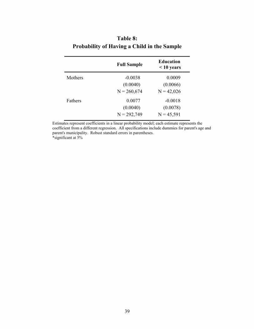
Table 8: Probability of Having a Child in the Sample

Full Sample Education < 10 years

Mothers -0.0038 0.0009 (0.0040) (0.0066) N = 260,674 N = 42,026

Fathers 0.0077 -0.0018 (0.0040) (0.0078) N = 292,749 N = 45,591

Estimates represent coefficients in a linear probability model; each estimate represents the coefficient from a different regression. All specifications include dummies for parent's age and parent's municipality. Robust standard errors in parentheses. *significant at 5%

39

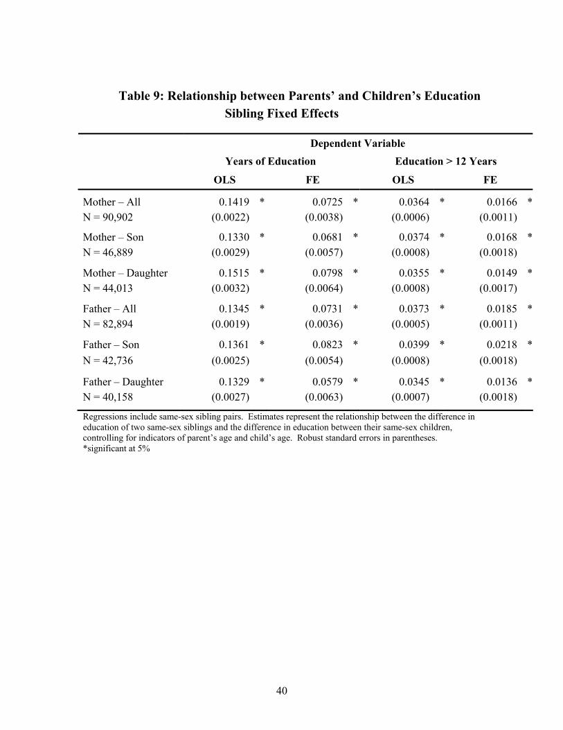
Table 9: Relationship between Parents’ and Children’s Education Sibling Fixed Effects

Dependent Variable

Years of Education Education > 12 Years

OLS FE OLS FE

Mother – All 0.1419 * 0.0725 * 0.0364 * 0.0166 *N = 90,902 (0.0022) (0.0038) (0.0006) (0.0011)

Mother – Son 0.1330 * 0.0681 * 0.0374 * 0.0168 *N = 46,889 (0.0029) (0.0057) (0.0008) (0.0018)

Mother – Daughter 0.1515 * 0.0798 * 0.0355 * 0.0149 *N = 44,013 (0.0032) (0.0064) (0.0008) (0.0017)

Father – All 0.1345 * 0.0731 * 0.0373 * 0.0185 *N = 82,894 (0.0019) (0.0036) (0.0005) (0.0011)

Father – Son 0.1361 * 0.0823 * 0.0399 * 0.0218 *N = 42,736 (0.0025) (0.0054) (0.0008) (0.0018)

Father – Daughter 0.1329 * 0.0579 * 0.0345 * 0.0136 *N = 40,158 (0.0027) (0.0063) (0.0007) (0.0018)

Regressions include same-sex sibling pairs. Estimates represent the relationship between the difference in education of two same-sex siblings and the difference in education between their same-sex children, controlling for indicators of parent’s age and child’s age. Robust standard errors in parentheses. *significant at 5%

40

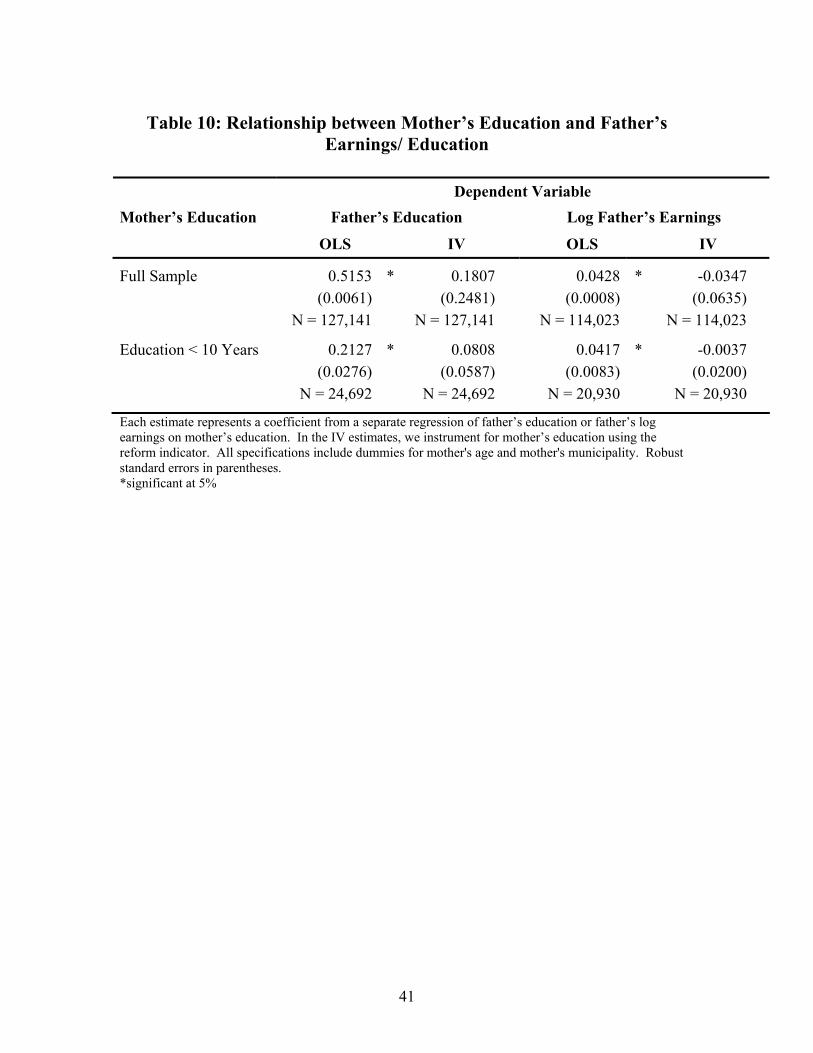
Table 10: Relationship between Mother’s Education and Father’s Earnings/ Education

Dependent Variable

Father’s Education Log Father’s Earnings Mother’s Education

OLS IV OLS IV

Full Sample 0.5153 * 0.1807 0.0428 * -0.0347 (0.0061) (0.2481) (0.0008) (0.0635) N = 127,141 N = 127,141 N = 114,023 N = 114,023

Education < 10 Years 0.2127 * 0.0808 0.0417 * -0.0037 (0.0276) (0.0587) (0.0083) (0.0200) N = 24,692 N = 24,692 N = 20,930 N = 20,930

Each estimate represents a coefficient from a separate regression of father’s education or father’s log earnings on mother’s education. In the IV estimates, we instrument for mother’s education using the reform indicator. All specifications include dummies for mother's age and mother's municipality. Robust standard errors in parentheses. *significant at 5%

41

Table 11: Relationship between Number of Children and Mother’s Education

Dependent Variable: Number of Children OLS IV

Mother’s Education 0.0014 -0.0185 Full Sample (0. 0015) (0 .0789) N=165,448 N=165,448 Mother’s Education -0.0296 * -0.0039 Education < 10 Years (0.0087) (0.0210) N=33,787 N=33,787

Each estimate represents the coefficient from a separate regression of number of children on mother’s education. All specifications include dummies for mother's age and mother's municipality. Robust standard errors in parentheses. *significant at 5%

42

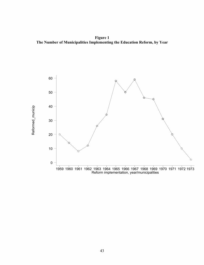
Figure 1

The Number of Municipalities Implementing the Education Reform, by Year

Ref

orm

ed_m

unic

ip

Reform implementation, year/municipalities1959 1960 1961 1962 1963 1964 1965 1966 1967 1968 1969 1970 1971 1972 1973

0

10

20

30

40

50

60

43

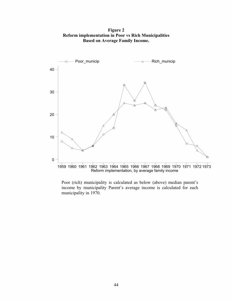
Figure 2 Reform implementation in Poor vs Rich Municipalities

Based on Average Family Income.

Reform implementation, by average family income

Poor_municip Rich_municip

1959 1960 1961 1962 1963 1964 1965 1966 1967 1968 1969 1970 1971 1972 1973

0

10

20

30

40

Poor (rich) municipality is calculated as below (above) median parent’s income by municipality Parent’s average income is calculated for each municipality in 1970.

44

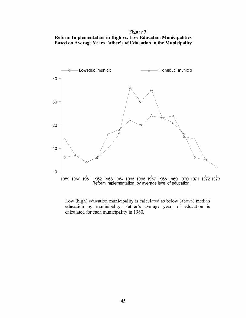
Figure 3 Reform Implementation in High vs. Low Education Municipalities Based on Average Years Father’s of Education in the Municipality

Reform implementation, by average level of education

Loweduc_municip Higheduc_municip

1959 1960 1961 1962 1963 1964 1965 1966 1967 1968 1969 1970 1971 1972 1973

0

10

20

30

40

Low (high) education municipality is calculated as below (above) median education by municipality. Father’s average years of education is calculated for each municipality in 1960.

45

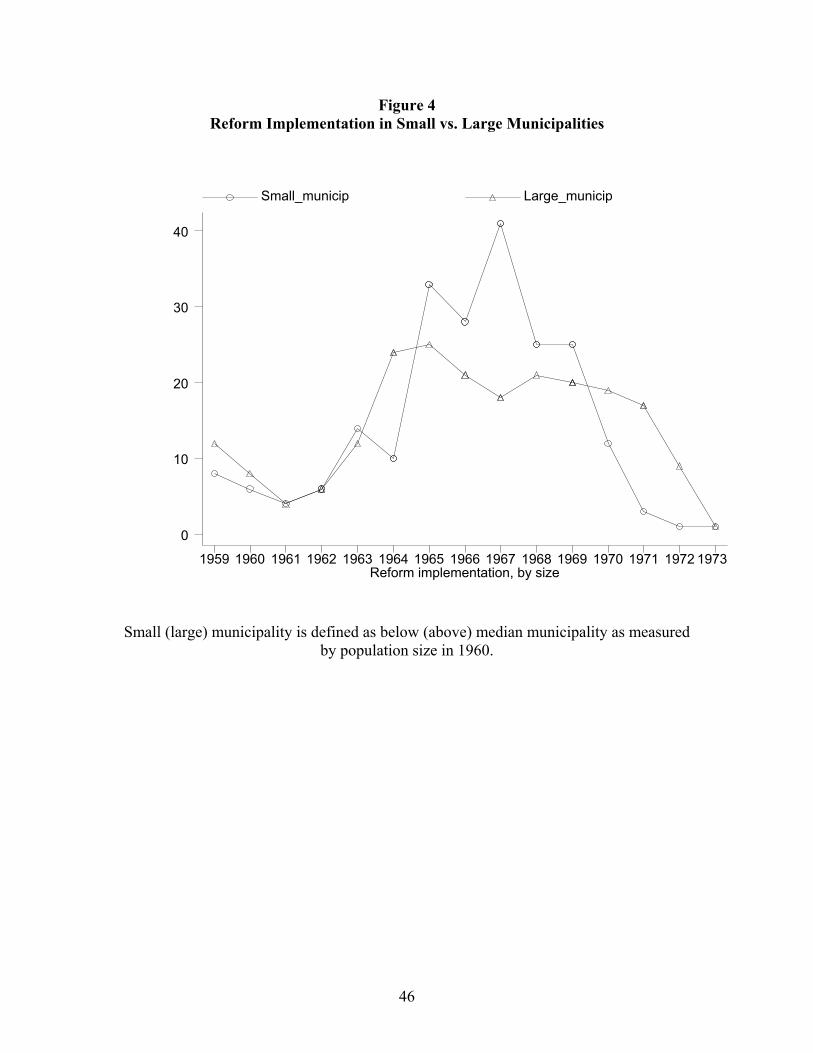
Figure 4 Reform Implementation in Small vs. Large Municipalities

Reform implementation, by size

Small_municip Large_municip

1959 1960 1961 1962 1963 1964 1965 1966 1967 1968 1969 1970 1971 1972 1973

0

10

20

30

40

Small (large) municipality is defined as below (above) median municipality as measured

by population size in 1960.

46

47

Appendix Table 1: Timing of the Implementation of the Reform

Dependent Variable: Year of Reform Coefficient Standard error County2 -1.95 .65 County3 5.02 5.23 County4 -.64 .70 County5 -.88 .67 County6 -.90 .62 County7 -1.21 .63 County8 -1.90 .64 County9 -1.21 .64 County10 -2.20 .71 County11 -.54 .63 County12 -1.4 .60 County13 -.45 .70 County14 1.23 .59 County15 -1.54 .58 County16 .04 .60 County17 -1.21 .57 County18 -.26 .65 County19 -2.77 .71 Share of Fathers with Some College

.92 3.88

Share of Mothers with Some College

12.30 8.31

Father’s Income (mean) -.007 .004 Mother’s Income (mean) -.01 .01 Father’s Age (mean) .11 .16 Mother’s Age (mean) -.12 .19 Size of Municipality/100 -.03 .03 Unemployment Rate 1960 -6.22 11.63 Share Workers in Manufacturing 1960

1.15 3.05

Share Workers in Private Services 1960

5.95 6.23

Share Labour Vote 1961 2.34 2.19 Constant term 1969.14 6.95

Robust standard errors. All variables are municipality level variables.

IZA Discussion Papers No.

Author(s) Title

Area Date

912 D. Checchi A. Filippin

An Experimental Study of the POUM Hypothesis 1 10/03

913 S. Pivnenko D. DeVoretz

The Recent Economic Performance of Ukrainian Immigrants in Canada and the U.S.

1 10/03

914 A. R. Cardoso P. Portugal

Bargained Wages, Wage Drift and the Design of the Wage Setting System

5 10/03

915 R. Hujer C. Zeiss

Macroeconomic Impacts of ALMP on the Matching Process in West Germany

6 10/03

916 S. C. Wolter S. Mühlemann J. Schweri

Why Some Firms Train Apprentices and Many Others Do Not

5 10/03

917 R. Euwals H. Roodenburg

A Note on the Redistributive Effect of Immigration

1 10/03

918 V. Jakobsen M. Rosholm

Dropping out of School? A Competing Risks Analysis of Young Immigrants’ Progress in the Educational System

1 10/03

919 M. Fertig

The Impact of Economic Integration on Employment – An Assessment in the Context of EU Enlargement

2 10/03

920 Ø. A. Nilsen K. G. Salvanes F. Schiantarelli

Employment Changes, the Structure of Adjustment Costs, and Plant Size

1 11/03

921 P. Egger M. Pfaffermayr A. Weber

Sectoral Adjustment of Employment: The Impact of Outsourcing and Trade at the Micro Level

2 11/03

922 J. Merz D. Burgert

Working Hour Arrangements and Working Hours – A Microeconometric Analysis Based on German Time Use Diary Data

5 11/03

923 U. Dulleck P. Frijters R. Winter-Ebmer

Reducing Start-Up Costs for New Firms: The Double Dividend on the Labour Market

5 11/03

924 A. P. Damm M. Rosholm

Employment Effects of Dispersal Policies on Refugee Immigrants, Part I: Theory

1 11/03

925 A. P. Damm M. Rosholm

Employment Effects of Dispersal Policies on Refugee Immigrants, Part II: Empirical Evidence

1 11/03

926 S. E. Black P. J. Devereux K. G. Salvanes

Why the Apple Doesn’t Fall Far: Understanding Intergenerational Transmission of Human Capital

5 11/03

An updated list of IZA Discussion Papers is available on the center‘s homepage www.iza.org.