Why So Many Local Entrepreneurs?∗

Claudio Michelacci†

CEMFIOlmo SilvaCEP and EUI

February 2006

Abstract

We document that the fraction of entrepreneurs who work in the region wherethey were born is significantly higher than the corresponding fraction for depen-dent workers. This difference is more pronounced in more developed regions andpositively related to the degree of local financial development. Firms created bylocals are more valuable and bigger (in terms of capital and employment), operatewith more capital intensive technologies, and are able to obtain greater financingper unit of capital invested, than firms created by non-locals. This evidence sug-gests that there are so many local entrepreneurs because locals can better exploitthe financial opportunities available in the region where they were born. This canhelp in explaining how local financial development causes persistent disparities inentrepreneurial activity, technology, and income.

JEL classification: J23, O12, O16, Z13Key words: Entrepreneurship, Economic and Financial Development, Social Capital

∗We owe much gratitude to Luigi Guiso for help with the data. We thank Francesco Daveri, AndreaIchino, Esteban Jaimovich, Omar Licandro, Steve Machin, Barbara Petrongolo, Dani Rodrik (the Edi-tor), Guido Schwerdt, and two anonymous referees for very helpful comments and suggestions. We alsobenefited from the comments of participants to seminars at EUI, LSE, UCL, the EEA Annual Conferencein Amsterdam, and the ESSLE meeting in Ammersee.

†Address for correspondence: Claudio Michelacci, CEMFI; Calle Casado del Alisal, 5; 28014 Madrid;SPAIN. Email: c.michelacci@cemfi.es.

1 Introduction

As emphasized by Schumpeter (1911), entrepreneurship is a key determinant of one econ-

omy’s technological performance.1 Entrepreneurship can be either nurtured locally or

attracted from abroad and, in principle, both sources of entrepreneurial activity can con-

tribute to technology growth. Yet their relative importance and determinants are largely

unexplored. In this paper, we document the relevance of local entrepreneurship for busi-

ness creation: we show that new businesses are mainly created by local entrepreneurs,

and that this tendency is more pronounced in more developed regions. We also analyze

the determinants of local entrepreneurship, and how it differs from other entrepreneurial

forms. Overall, our analysis suggests that entrepreneurship can hardly be regarded as a

mobile factor of production that gets allocated to arbitrage away technology differences,

and it identifies local entrepreneurship as a potentially relevant source of the well doc-

umented disparities in entrepreneurial activity, technology, and income, across countries

and regions (see for example Lucas, 1990 and Hall and Jones, 1999).

We document the contribution of local entrepreneurship to business creation, both in

the US and Italy. US data comes from the US Census 2000, which provides information

on both State of birth and State where the individuals currently work. Italian data

comes from the Survey of Household Income and Wealth (SHIW), which has recently

been used to analyze the effects of social capital on financial development and of local

financial development on real economic activity (see Guiso et al., 2004a and 2004b). We

evaluate the relevance of local entrepreneurship in different regions within a country, and

relative to other workers. This allows us to control for possible differences in judicial and

legal systems (which vary little within a country), as well as for any other institutional

and cultural characteristics that affect both entrepreneurial opportunities and individuals’

geographical mobility. In both the US and Italy we find that the fraction of entrepreneurs

who start-up their business in the region where they were born is significantly higher than

1Michelacci (2003) and Acs et al. (2004) formally analyze the role of entrepreneurship in endogenousgrowth models. They argue that entrepreneurship is the key factor that allows scientific knowledge toaffect technology. See Acs and Audretsch (2003) for a review on the literature documenting the existingpositive link between entrepreneurial activity and one country’s ability to achieve prosperity.

1

the corresponding fraction for dependent workers. We refer to this difference as a local

bias in entrepreneurship (LBE). Although Americans are substantially more mobile than

Italians, we find that the magnitude of LBE is comparable in the US and in Italy.

The Italian data contains detailed information on value, size, and financial structure

of businesses created by entrepreneurs. As this information is not available in the US

data, we analyze the determinants of LBE by focusing the analysis on Italy.2 We then

document the following empirical regularities:

1. LBE is more pronounced for larger businesses (in terms of market value and number

of employees).

2. LBE is positively related to the level of economic development of the region, as

measured by GDP per capita and the unemployment rate. Yet, it is almost unrelated

to the degree of specialization of entrepreneurial activities and their density.

3. Firms created by locals are bigger (in terms of market value, number of employees,

and capital), operate with more capital intensive technologies, and receive greater

financing per unit of capital invested, than firms created by non-locals.

4. LBE is increasing in the degree of local financial development, as measured by

Guiso et al. (2004a). This result holds after we instrument financial development

with some variables describing regional characteristics of the banking system as of

1936–thus just before a banking law was passed that strictly restricted entry in the

banking sector up to the mid-1980s; see Guiso et al. (2004a).

5. LBE is increasing in some outcome-based measures of trust in the community, such

as electoral participation and blood donation; see Guiso et al. (2004b). LBE appears

instead to be unrelated to measures of the importance of personal contacts in local

markets.2Italy is a country which has been unified, from both a political and a regulatory point of view, for

the last 140 years; yet, it still exhibits remarkable regional differences in technology and GDP per capita,which makes it particularly suitable for our investigation. Moreover, Italy is the country first studied bysociologists to investigate the effects of trust and social capital on real economic activity; see Banfield(1968) and Putman (1993).

2

As documented by, among others, Blanchflower and Oswald (1998), Evans and Jo-

vanovic (1989) and Holtz-Eakin et al. (1994), funds provision is an important concern

when creating a new business. We therefore interpret the previous findings as suggesting

that LBE results from the combination of two factors, independently put forth in the

literature. First, distance matters in the provision of funds, so that firms have to locate

close to their financiers to obtain financing. Berger et al. (2001) and Petersen and Rajan

(2002) provide direct evidence about the importance of distance in the provision of funds

to firms; a theoretical argument is given by Williamson (1987). Second, locals may have

some sort of “regional specific collateral” that facilitates access to credit and that would

be lost if they had to move and set-up their business in a different location. For example,

local financiers, such as banks and venture capitalists, may have privileged information

about individuals who have been living in a given location for several years. Or it could

be that moral hazard problems associated with borrowing are less severe, due to peer

effects or local social pressure, for individuals who reside in the same region as where they

were born; see Arnott and Stiglitz (1991) for a theoretical analysis of how peer monitoring

mechanisms can mitigate moral hazard problems. This mechanism would explain both

why local financial development benefits proportionally more locals than foreigners (Fact

4), and why local start-ups are bigger, more leveraged and operate with more capital

intensive technologies (Fact 3). Moreover, since trust appears to be one key determinant

of financial development (see Guiso et al., 2004b), this channel can also explain why LBE

is positively related to measures of trust (Fact 5).

Of course, there are other possible explanations for LBE.3 These however seem to

contradict some of the previous findings. For example, LBE could arise if individuals

choose to become entrepreneurs in their native location because they strongly prefer to

reside there, but they lack of employment opportunities as dependent workers. Alba-

Ramirez (1994), Martinez-Granado (2002), and Chelli and Rosti (1998) document how

this may explain some entrepreneurial spells in Spain, UK, and Italy, respectively. If

3See Section 2 of the working paper version of this study for a simple model, based on Lucas (1978),describing how the different mechansims discussed in the text can induce LBE.

3

this was the main explanation for LBE, however, we would expect a negative correlation

between LBE and the local level of development: in particular LBE should be inversely

related to the unemployment rate in the region of residence, which does not appear to

be the case (Fact 2). This possible explanation also seems at odds with the finding that

locals create more valuable businesses than non-locals (Fact 3).

Alternatively, the combination of entrepreneurial learning and regional sectoral spe-

cialization may provide an explanation for LBE. Consider a situation where regions tend

to have a natural advantage in some sectors of activity, and that entrepreneurs choose to

start-up their business in the region with the greatest natural advantage in the business

sector. Also assume that, due to learning and technological spill-overs, local individuals

have a greater probability than non-locals of acquiring entrepreneurial ideas specific to

the sector where the region has its natural advantage. This mechanism would also induce

LBE. Guiso and Schivardi (2005) provide some evidence supporting the relevance of this

channel. Yet, our results suggest that entrepreneurial learning can hardly account for

the previous findings. In particular this explanation would tend to predict that LBE is

greater in regions where the sectoral natural advantage and the scope for learning from

other entrepreneurs are greater. Fact 2 documents that LBE is only mildly related to the

degree of sectoral specialization of entrepreneurial activities and to the number of entre-

preneurs present in the regions of birth. This seems to limit the scope of an explanation

based on the combination of entrepreneurial learning and regional sectoral specialization.

Finally, LBE could arise because locals can better exploit their personal network to

contact customers and suppliers, to obtain more reliable information about the company’s

business market, or to more easily recruit workers in labour markets.4 Thus we would

expect LBE to be positively related to measures of social capital, and of intensity of

personal networks in the local community.5 Fact 5 documents that LBE is higher in

4The idea that personal networks and social capital matter in business formation has been emphasizedby Aldrich and Zimmerman (1986). Aldrich et al. (1987) and Blumberg and Pfann (2001) provide someevidence that entrepreneurs heavily rely on their personal networks to start up their business, and makeit succeed. The role of social contacts in the labor markets has also been recognized by, among manyothers, Granovetter (1974), Montgomery (1991), and Bentolila et al. (2004).

5See Coleman (1988) and (1990) for a definition of social capital, which is described as a resource for

4

regions with higher level of trust; however, this is unrelated to measures of the importance

of social contacts in local markets. Since LBE is also positively related to the degree of

local financial development (Fact 4), overall we find some evidence that social capital

contributes to business formation, at least because it facilitates access to credit for local

entrepreneurs.

The paper is organized as follows. Section 2 describes the Italian dataset. Section

3 documents LBE in Italy and the US. Section 4 uses Italian data to document some

properties of LBE. Section 5 discusses the role of local credit markets, while Section 6

deals with social capital. Section 7 concludes.

2 Data

Since our analysis mainly focuses on Italy, we start describing the Italian data and then

discuss how well it represents the population of Italian firms. We will briefly describe the

US Census data later, when using it.

2.1 Description

Italian data primarily comes from the Survey of Household Income and Wealth (SHIW)

collected by the Bank of Italy. SHIW provides a representative picture of Italian house-

holds, both in terms of income dynamics and occupational choices. We focus on the 1991,

1993, and 1995 waves of the Survey because they contain detailed information on indi-

vidual decisions about occupational choice and geographical mobility. We only sample

working individuals aged between 18 and 65, who are heads of household. Heads of house-

hold are the most relevant decisional unit within a household and they are most likely

to actively engage in the labour market; this reduces sample selection problems related

to labor market participation.6 Further details about the construction of the dataset and

the definition of the variables used in the analysis are contained in the Appendix.

action, accruing to individuals embedded in social ties, that facilitates productive activities.6We also drop individuals born in the Aosta Province. In fact, no people living in that Province were

interviewed in any SHIW waves implying that no information about geographical mobility is available.

5

We start constructing the variable Local as a dummy variable taking value one if the

individual works in the Province where she was born.7 Italy is currently divided in 20

Regions and 103 Provinces. An Italian province roughly corresponds to a US county.

Individuals sampled in SHIW are asked to report about their main working activity.

First, they have to state whether they work as dependent workers or self-employed. If

dependent workers, they then report whether they work as blue or white collars. If self-

employed, they report whether they are 1) entrepreneurs, 2) craftsmen, 3) professionals,

4) manager/partners of societies, and 5) workers of family firms. We construct the vari-

ableWorker as a dummy variable identifying individuals who work as dependent workers

(either blue or white collars). We then construct the variable Entrepreneur as a dummy

variable identifying self-employed with some salient traits typically associated with entre-

preneurship, such as risk bearing, independence in decision making, innovative behavior,

and creative attitude. To decide which self-employed worker is an entrepreneur, we rely

on the Survey explanatory notes and we classify as Entrepreneur any self-employed who

works as either 1) entrepreneur, 2) craftsman, 3) professional, or 4) manager/partner of

societies. Indeed, according to SHIW explanatory notes, both entrepreneurs and crafts-

men actively and personally manage the business that they own; the main difference

between the two occupations is related to the number of people employed in the activ-

ity, with craftsmen mainly working alone. Similarly, manager/partners of societies are

defined as individuals who own shares of the firm and who actively run and manage

the business. We also include professionals in the definition of Entrepreneur, since this

category includes any individual who independently practises her art or profession, and

who usually remains personally liable for her business activity.8 Conversely, we exclude

self-employed workers of family firms from the definition. In fact, workers of family firms

7We assume that individuals work and live in the same Province as no information about workinglocation is available. To check for the validity of this assumption, we also ran all the analysis using Regionsrather than Provinces to identify geographic mobility, see Table 4. As Regions cover large portions of theItalian territory, it is unlikely that individuals live and work in different Regions. Results remain broadlyunchanged, which makes us confident about the plausibility of the assumption.

8Yet, this last choice may be more controversial, since business creation is not always clearly associatedwith becoming a professional. Therefore we checked that excluding professionals from the definition ofEntrepreneur does not affect the results below. In order to save space, we do not report the results.

6

are mainly just workers, classified as self-employed, who contribute to the activity of the

family venture. In many cases, however, these jobs require little leadership and innovative

activity, which justifies their exclusion.9

It is widely documented that entrepreneurs are very likely to be children of entre-

preneurs (see, for example, Dunn and Holtz-Eakin (2000) and references therein). This

is an important concern if second generation entrepreneurs simply take-up the business

activities started by previous generations. As the physical structures of the ventures can

be not be very easily relocated, the geographical mobility of entrepreneurs could appear

to be low simply because businesses are mechanically passed down from one generation

to the next. To mitigate this problem, we construct the variable Start-up as a dummy

variable identifying individuals who start-up a new business. We use information about

the channel whereby a job was found, and we classify as start-ups all Entrepreneurs who

declare that they have not obtained their job “by taking up parents’ activities” (Start-

up).10 Questions about the channel whereby a job was found were not asked in 1995. To

increase the degrees of freedom, in some of the specifications below we also add data for

1995. In that case we identify as start-ups those Entrepreneurs who are not working in

the same occupation and sector as the one of their parents. This is quite restrictive in

distinguishing start-ups from other entrepreneurs, since in principle new ventures could

be created in the same sector and occupation as that of the parents. Finally, the dummy

variable Non Start-up identifies Entrepreneurs who are not start-ups.

For our analysis, we also use information about individuals’ Gender, Age, Educational

achievements, Marital status, Number of children, Household Wealth and Income, Job

Tenure, and, for start-up entrepreneurs, Firm Age. Descriptive statistics for the variables

retained in the analysis are reported in Table 1. SHIW also provides information about

9As a result, we also exclude workers of family firms from the sample, as it would be misleading toconsider them as dependent workers either.10We also checked that our results remain unchanged when defining as Start-up any Entrepreneur who

declares that she has found her job by “having started an activity on her own”. The correlation betweenthe two definitions is very high (close to ninety per cent). With this second definition, however, we maymiss out some new entrepreneurial ventures that take the form of a large incorporated company, since,in this case, it is not clear how the individual would interpret the wording of the question.

7

the monetary value of entrepreneurial ventures, as well as other measures of firm’s size.

Entrepreneurs in SHIW are asked to estimate the market value of their participation in the

venture, in case of selling it. This is the basis to calculate Firm’s Market Value. We also

consider indicators for the Employment Size of the firm, for the Capital Stock and for the

Capital-Labor ratio. To measure the capital stock of the firm we use information about

capital depreciation, which corresponds to the variable Ammortamenti in the Survey.

Ammortamenti is the amount of capital that has to be imputed by law to the current

year of production. This legal requirement is set taking into account sector of activity,

age, and legal structure of business ventures and it represents a proxy for the capital

stock of the firm. To have a proxy for the capital-labor ratio, we divide the value of

“Ammortamenti” by the number of people working at the firm.

All variables characterizing the size of the firm (in terms of value, employment or

capital) are self-reported and thus likely to be subject to measurement error. The Em-

ployment Size of the firm is less likely to be subject to under-reporting than Firm’s Value,

which tends to be understated for fear that statistical information may be leaked to the

tax authority; see OECD (1992) and (2000) for evidence about this.

2.2 Is the Italian sample representative?

Since SHIW was not designed to be representative of the population of Italian firms (but

just of Italian households), we start assessing how well the characteristics of the ventures

sampled in SHIW track features of the population of Italian firms. We compare some

sample statistics from SHIW with similar records obtained from ISTAT 1991 Census of

Italian Firms and Services. We study firms’ characteristics along the size and geographical

location dimensions since they are key for the analysis that follows. We also discuss some

evidence about the sectoral distribution of firms sampled in SHIW, which is also relevant

for some of the exercises pursued below. It is worth mentioning that ISTAT Census only

marginally covers agricultural activities. This may partly alter the comparability of the

two samples. For this reason, we report figures both including and excluding agricultural

activities from computations.

8

Table A1 in the Appendix compares the size distribution of firms in the two datasets.

ISTAT data show that Italian firms tend to be quite small.11 SHIW reproduces this

feature remarkably well and independently of the exclusion of the agricultural sector from

the analysis. The Table also reveals that the geographical distribution of firms in SHIW

tracks closely that obtained by using Census data.12 The only remarkable exception is

Lombardia, which is one of the most heavily industrialized Regions in Italy: although

Lombardia is the Region with the greatest number of firms in both datasets, its absolute

relevance is more striking in ISTAT data than in SHIW. This is probably due to the fact

that Lombardia is a Region where many foreign and multinational firms are located. Since

SHIW only sample Italian individuals, foreign owned businesses are not in our dataset.

While this may explain the observed discrepancy, it might also bias our analysis since

it may lead us to underestimate the geographical mobility of entrepreneurs by omitting

an important component of the entrepreneurial pool. As long as the difference between

ISTAT and SHIW firms’ geographical distribution captures the incidence of foreign and

multinational firms, this measure can be used to assess the robustness of our findings. In

the analysis that follows, we check that our results are not driven by omitting foreign and

multinational firms from our sample. Finally, when we compare the sectoral distribution

of firms in SHIWwith that in ISTAT Census, we find that SHIW slightly under-represents

Trade and Commerce, while it over-represents Manufacturing; yet, overall, the two surveys

provide a very similar picture of the sectoral composition of Italian firms.

3 Evidence of LBE

We start documenting the existence of LBE both in Italy and in the US.

11For the sake of comparison, notice that 75% of US firms have between 1 and 9 employees, that 12%have between 10 and 19 employees and that 13% have at least 20 employees. See US Census BureauData, 2001 at: https://www.sba.gov/advo/stats/data.html12We also assessed the geographical distribution of firms by Province. The results are in line with those

obtained using Regions. They are not reported here to save space.

9

3.1 Basic evidence

To measure the magnitude and significance of LBE we run the following regression:

Locali = ω + λEni + δXi + εi

where, as previously discussed, Locali is a dummy variable taking value one if individual i

works in the province where she was born, while Eni is a dummy variable taking value one

for individuals who are either Entrepreneurs or Start-ups, depending on the specification.

Whenever Eni identifies start-up entrepreneurs, we include in the vector of controls a

dummy for Non Start-up entrepreneurs. As a result, the intercept ω identifies the fraction

of dependent workers (Workers) working in the province where they were born; the λ

coefficient instead measures LBE for either Entrepreneurs or Start-ups. Finally, the vector

Xi includes a set of individual and aggregate control variables, that vary depending on

the specification. Our approach is thus descriptive: it allows quantifying the difference

between the fraction of local entrepreneurs and local dependent workers, after controlling

for some relevant characteristics. Since the main variables of interest vary at the Province

level, in all regressions, we correct standard errors for possible dependence of residuals

within Province clusters.

3.2 LBE in Italy

We start by considering the sample only concerning 1991 and 1993. Table 2 reports the

fraction of local dependent workers (i.e. the constant ω) and the local bias in entrepre-

neurship, using different definitions and specifications. Columns 1 and 2 quantifies LBE

when comparingWorkers to Entrepreneurs, with and without controlling for the following

characteristics: age, gender, four dummies for educational achievements, marital status

and number of children; five macro region dummies (North-West, North-East, Center,

South and Islands); and a full set of year dummies.13 This set of regressors is included

to assure that some basic individual and aggregate attributes do not drive our findings.

13As a robustness check, we also augmented our regressions with industry dummies. The results wereunchanged.

10

Columns 3 and 4 quantify LBE when considering Start-ups rather than Entrepreneurs.

Finally, in Column 5 we break up the share of local dependent workers into white and

blue collars, and quantifies LBE relative to each group.

The size of LBE is around 7 percentage points. This is the result of the difference

between a share of local Entrepreneurs which is around 79%, and a share of local dependent

workers, which is around 72%. These numbers are quite high, which suggests that LBE

cannot be disregarded on the basis of its little economic relevance. LBE does not vary

substantially after controlling for individual characteristics and it arises independently of

whether we focus on Entrepreneurs or Start-ups. This implies that the transmission of

entrepreneurial activities from one generation to the next is unlikely to explain LBE.14

When the fraction of dependent workers is split into white and blue collars (Column 6),

we find that LBE for Start-ups is about 7 percentage points with respect to white collars,

and 4.5 percentage points (but still highly significant) relative to blue collars. When

considering Non Start-up entrepreneurs the effects are approximately twice as big.

In Table 3 we show that the previous findings remain broadly unchanged when adding

the third SHIW wave. Columns 1 and 3 of Table 3 reveal that LBE is in the order of 6.5

to 7.5 percentage points when no controls are used. After adding the controls (Columns

2 and 4), we still find that LBE is positive, statistically significant and of a similar order

of magnitude. Given that the inclusion of the 1995 wave leaves the results unchanged, in

the remaining of the analysis we make use of all three SHIW waves, to increase degrees of

freedom. Moreover, we present only results pertaining to start-ups entrepreneurs. Indeed

start-ups provide the most direct evidence about business creation, which is the focus of

the paper.15

As previously discussed, the exclusions of foreign owned businesses from our dataset

may affect our results. To assess the robustness of our findings to this concern, we

measure the incidence of foreign and multinational firms in the region by calculating the

14Also notice that the problem of the intergenerational transmission of entrepreneurial activities isreduced by the fact that we excluded workers in family firms from the definition of Entrepreneur.15In any case, we checked that our findings remain valid when using all entrepreneurs rather than just

start-ups.

11

difference between ISTAT and SHIW firms’ geographical distribution. We then evaluate

how the inclusion of this control in our regressions affects LBE and, how it interacts with

it. Columns 6 of Table 3 reports on this exercise. Once we include the ISTAT-SHIW

discrepancy in the geographical distribution of business ventures and its interaction with

the entrepreneurial status variable, we find that LBE is as sizable and significant as

before. The interaction term is also positive, yet not strongly significant. Overall this

indicates that the omission of multinational and foreign owned businesses from the sample

is unlikely to drive our results.

3.3 Some evidence for the US

Italy is a country where geographical mobility is quite low. We now show that LBE also

exists in a more mobile economy such as the US. We use the US Census 2000—one-per-

cent file data. Census data are available at the Integrated Public Use Microdata Series

(IPUMS) centre at the University of Minnesota. Similarly to SHIW, the sampling unit

in Census 2000 is the household. Approximately 1 out of every 6 housing units in the US

were included in the long form Census 2000 sample. The one-per-cent sample produced

in 2000 is obtained by randomly selecting one per cent of the observations in the long

form Census 2000 sample. The data contains information on individual’s educational

achievement, marital status, age, race, occupational status, State of birth and State of

work.

Like in the SHIW analysis, we retain only heads of households aged between 18 and 65.

We only consider US citizens who are of either “White” or “Black and Afros” origins. We

drop US Natives, non US-citizens, and US citizens with other ethnic origins (mainly from

East Asia), because US Natives are a very small and peculiar group, displaying almost no

mobility rates, while non US-citizens and individuals with other ethnic origins are likely

to be born out of the US, independently of their occupation.

We construct the variable Local as a dummy variable taking value one if the individual

works in the US State where she was born. Since a US State is substantially larger than

an Italian Province, we compare US results with those obtained by using Italian Regions

12

(rather than Provinces) as the geographical unit of the analysis. Individuals sampled in

Census are asked to report about their main working activity. We select individuals who

are at work, and we construct the variable Worker as a dummy identifying individuals

working as dependent workers, in either the public or private sector. Next, the variable

Entrepreneur identifies self-employed workers in either incorporated or not incorporated

business. Notice that an incorporated business may better represent what may arguably

be considered a true entrepreneurial venture. For example, if there are some fixed costs

to incorporate a business, entrepreneurs would find it profitable to pay for them only

in the presence of sufficiently rewarding projects; so incorporated businesses tend to be

larger than not incorporated ones. In the following analysis, we report results for the two

separate categories. In all regressions we use a set of controls similar to those previously

considered; see the descriptive note in Table 4 and Table A2 for details.

Our findings are reported in Table 4. The first Column quantifies LBE in Italy when

using Regions to identify geographical mobility. LBE is around 5 percentage points, which

implies that entrepreneurs are approximately 6.5 less mobile than dependent workers. US

results are reported in Columns 2 to 5. Columns 2 and 3 deal with all selected individuals,

Columns 4 and 5 present results for Whites only. Columns 3 and 5 separately quantify

LBE for self-employed in incorporated and non incorporated businesses. American work-

ers appear to be substantially more mobile than Italian workers. Yet, LBE also arises in

the US economy. Its magnitude is similar when considering incorporated or non incor-

porated businesses. The estimated LBE for the US is about 3 percentage points, and it

is statistically significant. This implies that, in the US, entrepreneurs are about 4.5 per

cent less mobile than dependent workers. This is comparable with our Italian results.16

16In comparing the results one may also notice that a US State is still bigger than an Italian Region.Clearly the size of the geographical unit of analysis affects the mobility rates of workers and entrepreneurs.To control for this effect, we re-ran all the US regressions after adding a control for the population sizeof each US State. We found that the magnitude of LBE remained unchanged. This is in line with theItalian evidence, where LBE is not strongly affected by considering as a unit of analysis the Region ratherthan the Province.

13

4 More on LBE

Differently from the US data, SHIW contains detailed information on value, size, and

financial structure of the businesses created by entrepreneurs. Thus, we henceforth focus

the analysis on Italy. We next show how LBE relates to i) the size of the firm, ii) the

development of the region, and iii) the sectoral specialization of entrepreneurial activities.

4.1 LBE and firm’s size

Table 5 characterizes how LBE is related to the size of the firm. Panel A deals with

employment size. The first two Columns quantify LBE for firms employing one or more

than one worker; in the last two Columns, we repeat the exercise for firms employing

five or more than five workers, which corresponds to the top decile of the distribution

of employment size of firms in SHIW. We find that the share of local entrepreneurs is

always significantly higher than the share of local dependent workers. Moreover, LBE

is increasing in the number of people employed at the firm: LBE is between 10 and 11

percentage points when considering larger businesses.17

Panel B in Table 5 deals with the market value of the business. In the first two

Columns, we split the sample by using the median of the value distribution of firms

(which is equal to 30 millions of 1991 Italian liras). In the last two Columns, instead,

we use the top decile (which is equal to 300 millions of 1991 Italian liras). In any group

we find that the share of local entrepreneurs is higher than the corresponding share of

dependent workers. Interestingly, LBE is also increasing in the value of the firm: for start-

ups in the top decile of the distribution of firm’s values, LBE is as high as 10 percentage

points.

The findings presented in Table 5 highlight a positive relation between measures of

firm’s size and LBE. To corroborate the claim, we also compare the average size of local

and non-local firms. To do so, we consider i) the employment size of the firm, ii) the

capital stock, as proxied by yearly “Ammortamenti” (capital depreciation), and iii) the

17We also studied whether the fraction of local dependent workers varies in firms of different size. Wedid not find any significant pattern.

14

capital-labor ratio. For completeness, we also compare the average wage of local and

non-local dependent workers.

Table 6 reports the results obtained by regressing proxies for firm size and capital

intensity on a dummy identifying local entrepreneurs; Columns 2, 4, and 6 include the

following controls: individuals’ gender, age, family status, number of children, job tenure,

and average hours worked per week; indicators for the size of the city or town where

the individual lives; dummy variables for educational achievement, less than full year

activities, sector of occupation and calendar year; and five macro region dummies. We

find that firms managed by local entrepreneurs are larger in size and more capital intensive.

Given the average size of firms, the employment advantage of local start-ups is around 37

per cent. Similarly, local firms have, on average, 40 per cent more capital, and capital-

labor ratios which are 38 per cent higher than non-local firms.18 This may suggest that

locals have an advantage at creating a business in their native location. Of course, this

may also simply reflect selection issues, say because only the best businesses created by

locals survive and thrive.

We repeat a similar exercise for dependent workers, considering both their total wage

bills and their net wage income. We control for all variables included in the previous

regressions, and local unemployment rates. Results are reported in Table 7. A remarkably

different picture emerges: local dependent workers earn significantly lower total wage bills

and net wages, than migrants do. This is in line with findings in the migration literature;

see for example Borjas (1987) and Borjas et al. (1992). The wage premium of immigrants

is to be imputed to white collars immigrants, earning significantly more than local white

workers. Given the average total wage bill, local white collars earn 5 per cent less than

movers; a similar figure emerges when using net wages. Overall there exist remarkable

differences between dependent workers and entrepreneurs in that dependent workers who

migrate earn higher average wages than locals, while the businesses created by non-local

18We also repeated the same exercise using the pecuniary value of the firm. As already mentioned, thismeasure is subject to substantial under-reporting, especially at the top of the distribution. Also in thiscase, we find that local start-ups have higher pecuniary value than non-local ones although the differenceis somewhat less significant than that obtained with employment size and capital.

15

entrepreneurs are on average smaller and less valuable than those created by locals.

4.2 LBE and local economic development

So far, we have analyzed how the relative mobility of entrepreneurs is related to individual

and business characteristics. We next discuss how LBE is related to some measures of

local economic development such as unemployment rate and GDP per capita. Since these

indicators only vary across provinces (or regions), one caveat applies when evaluating

the statistical significance of the coefficients. Correcting standard errors for possible

dependence of residuals within Province (or Region) clusters is asymptotically efficient;

yet, as shown by Bertrand, Duflo, and Mullainathan, (2004), there may be problems in

finite samples. To investigate this issue, we follow Guiso et al. (2004a) and we also report

the P-values that arise when we collapse the data at the provincial (or regional) level, after

partialling out individual effects. The results appear in square brackets at the bottom of

Table 8. We proceed analogously in the rest of paper, when considering indicators that

exhibit no variation within a Province (or a Region).

Unemployment rates by Regions of residence were obtained from ISTAT Labor Force

Surveys for 1991, 1993, and 1995, and averaged over the three years.19 Since we are

interested in analyzing how labour market conditions affect LBE, we would like to use

the unemployment rate at the date when the business was created or the worker be-

come employed. These are however difficult to be imputed. Nevertheless, unemployment

differentials across Italian Regions have not (drastically) changed over the past decade.

Moreover, current average unemployment rates may provide a better approximation to

the life-time employment opportunities which affect individuals’ working choices. In Table

8 we first analyze the relation between local unemployment rates and LBE by interact-

ing the entrepreneurial status variable with local unemployment. Column 1 presents the

results with raw figures; Columns 2 includes the usual set of individual and aggregate

controls.19Unemployment rates defined over Provinces could not be computed as provincial codes in ISTAT-

Labor Force Surveys are protected for confidentiality reasons.

16

We find a negative relation between LBE and local unemployment rates. Indeed the

interaction term between the entrepreneurial status variable and the unemployment rate

displays a sizable, significant, negative coefficient, implying that in regions where unem-

ployment is lower, LBE is higher. An increase in the unemployment rate of 5 percentage

points is associated with a decrease in LBE of about 1.5 per cent for Start-ups.

As discussed in the Introduction, when employment opportunities as dependent work-

ers are scarce and people are attached to the native location, individuals may decide to

create their own business, which could in principle explains LBE. Yet, the evidence in the

first two Columns of Table 8 imply that LBE is higher in regions with more favorable la-

bor market conditions; this suggests that the combination of poor labor market conditions

and individuals’ attachment to the native location can hardly explain LBE. Furthermore

local businesses tend to be larger and more valuable than non-local ones, which further

suggests that this explanation can not fully account for LBE.

Columns 3 to 6 of Table 8 further characterize the relation between LBE and local level

of economic activity by studying how LBE varies across Italian regions (North vs. South)

and in relation to the Province level per capita GDP. Columns 3 and 4 provide evidence

that LBE is higher in the North than in the South. The regional breakdown roughly

reproduces Italian disparities in terms of economic activity, since Northern Regions are

among the richest areas in the European Union while Southern Regions are among the

poorest. Overall the evidence suggests that LBE tends to be positively related to the

level of economic activity.

Columns 5 and 6 provide further support to the claim, by relating LBE to the Province

level per capita GDP in 1970.20 The specific year is chosen because more than 70% of the

sampled entrepreneurs started their activity after 1970. This allows us to better isolate

the effect of exogenous variation in economic development on LBE since it reduces the

risk that the correlation is driven by the effects of entrepreneurial activity on local GDP.21

20We use raw GDP per capita, rather than its logarithm, to make results comparable with Guiso et al.(2004a). Results remain unchanged when considering the logarithm of per capita GDP rather than itslevel.21We also tried considering earlier years and averages over the 1965-1975 period. The results are

roughly unchanged; yet, earlier data include missing values and their reliability is somewhat reduced.

17

Results show that the interaction term between entrepreneurial status and per capita GDP

is positive and significant, which confirms that LBE is higher in more developed regions.

Overall the positive relationship between LBE and economic activity (as measured by

employment rates and GDP per capita) may indicate that local entrepreneurship plays a

role in creating persistent disparities in economic development.

4.3 LBE and local entrepreneurial density

In Table 9, we relate LBE to the entrepreneurial density in the Province of residence.

The idea is to investigate whether learning from other entrepreneurs could explain LBE.

For each Province considered in SHIW, we compute the fraction of entrepreneurs over the

population of residence in 1991, 1993, and 1995, and we proxy for the degree of entre-

preneurial density by taking the average figure over the three years. Results are reported

in Columns 1 and 2. Using information derived from various ISTAT data collections, we

also relate LBE to the ratio of firms in a Province to the population of the Province, in

1971. This year is sufficiently far away in time, that most entrepreneurs in our sample

had not yet started up their activity by that date, which reduces reverse causality prob-

lems. Results are reported in Column 3. Our findings show that there exists a positive

relation between LBE and the density of entrepreneurial activities. Yet, its effect is mod-

est in size and not robust. For example, after controlling for individual characteristics

in Column 2, the interaction term between the entrepreneurial status variable and our

measure of entrepreneurial density is not significantly different from zero. This may in-

dicate that technological spill-overs and learning from other entrepreneurs play little role

in determining LBE.

To further investigate the role of technological spill-overs in determining LBE, we

next relate LBE to the sectoral composition of local entrepreneurial activities. The idea

is to test whether technological spill-overs are stronger in Provinces where entrepreneurial

activity is more specialized. If technological spill-overs are the main explanation for LBE,

we would expect LBE to be increasing in the degree of specialization of entrepreneurial

activities. We measure the level of entrepreneurial specialization in a specific sector and in

18

a given Province, by computing the total number of entrepreneurs within a sector-Province

cell over the total number of entrepreneurs in the Province, which is similar to the proxy

used in Guiso and Schivardi (2005). We then take the average figure obtained over 1991,

1993, and 1995.22 In fact, we are unable to calculate the corresponding quantity at the

date when each business venture was actually started. Yet, the geographical and sectoral

distribution of the Italian districts have not drastically changed in the past decades,

which makes us confident about this measure of sectoral specialization of entrepreneurial

activities.

When we augment the regressions in Column 2 of Table 9 by including the indica-

tor for the sectoral composition of entrepreneurial activities and its interaction with the

entrepreneurial status variable, we find that the degree of entrepreneurial specialization

does not play any significant role in accounting for LBE (see Column 4). We even find

that LBE is lower in Provinces with more specialized entrepreneurial activities, although

the effect is not statistically significant.

Guiso and Schivardi (2005) show that in areas with dense and specialized entrepre-

neurial environments, average total factor productivity tends to be higher. They argue

that when more entrepreneurs work within a given sector and geographical area, peo-

ple have higher chances of acquiring specific entrepreneurial skills.23 Although they do

not directly address the question of why LBE may emerge, their evidence could suggest

that technological spill-overs and entrepreneurial learning may explain LBE. Our findings

however provide little support to this explanation.

5 The role of financial markets

It is well documented that funds’ provision is an important concern in the decision to

become an entrepreneur. As discussed in the Introduction, there are several reasons why

22Guiso and Schivardi (2005) use the number of entrepreneurs in a sector-Provice cell over the totalpopulation to measure entrepreneurial density. Our results do not vary when considering this alternativeproxy.23A closely related strand of literature focuses on knowledge and R&D spill-overs and location decisions,

suggesting that business ventures tend to be concentrated in locations specialized in given productionactivities, see e.g. Ellison and Glaser (1997).

19

locals could have a better access than non-locals to local credit markets. If firms also have

to locate close to their financiers to obtain credit, this mechanism could explain why LBE

emerges. We therefore now investigate the role of financial markets in determining LBE.

We start documenting that local firms are able to obtain greater financing per unit of

capital invested. Then, we construct an index of local financial development, and relate

it to LBE, the probability of being an entrepreneur, and to firm’s size.

5.1 Preliminary evidence

Table 10 documents that firms created by locals receive greater financing per unit of

capital invested, than firms created by non-locals. We consider the sample of start-up

entrepreneurs, and regress the ratio of bank debts to firm’s capital on the dummy for

being a local. In column 2 we report the results after including the usual set of variables.

Bank debts are measured in SHIW as short term (within 18 months) debts towards banks

and other financial institutions, that pertain to the business activity.

We find that the dummy identifying local individuals displays a positive and significant

coefficient. Given average values for the bank debt-capital ratio, this implies that local

entrepreneurs obtain 45 per cent more financing per unit of capital invested than non-local

entrepreneurs.

5.2 An index of local financial development

To further investigate the role of financial markets, we follow Guiso et al. (2004a) in

constructing a measure of local financial development. We exploit information collected

in SHIW about households’ access to credit. SHIW asks to report whether the household

has been turned down for a loan or discouraged from applying; we use this information

to create an indicator measuring how easy it is to obtain credit in a given location.

To apply the methodology we have to take a stand on what is the relevant local

financial market. Ideally, we would like to construct Province level indicators as this

would be consistent with the evidence discussed so far. Moreover, up to the ’90s, banks

could only open branches conditional on authorization granted Province-by-Province by

20

the Bank of Italy. Thus, also from an economic point of view, the Province seems to

be the natural unit of analysis. Yet, as documented in Guiso et al. (2004a), statistical

considerations related to missing data suggest that regional indicators are more reliable.

We therefore compute and report results obtained using both Province- and Region-level

indicators.

To identify geographical differences in the supply of credit, we estimate the probability

that a household, potentially interested in borrowing, is either turned down for a loan

or discouraged from applying. To approximate the set of potential borrowers we pool

together all households with some debt and those that we know have been denied credit

or discouraged from applying for a loan. We then estimate a linear probability model for

the likelihood that a household is shut off from the credit market–i.e. it has either been

denied a loan or discouraged from applying. As controls we include: household income

and wealth (linear and squared); number of people belonging to the household, number

of children; household head’s age, gender, marital status, educational achievement and

job qualification; indicators for the size of the city or town where the household lives

and calendar year dummies. Finally, we include dummy variables for either Provinces or

Regions of residence. Region and Province dummies represent the conditional probability

of being shut off from the credit market in the corresponding location. We then use

these conditional probabilities to measure local financial development by computing the

following indicator:

Kav = 1− Conditional Probability of Rejectionmax {Conditional Probability of Rejection}

where Kav stands for capital availability. We denote Province- and Region-level credit

availability by KavP and KavR, respectively.

To support the validity of the indicators we report on three exercises. First, an F-test

strongly rejects the null hypothesis that either the Province or the Regional dummies are

all equal. Second, a test on whether dummies for Provinces within the same Region are

equal leads to a rejection of the null hypothesis in only two Regions (corresponding to

Lombardia and Toscana) out of 19. Finally, we checked that there exists a significant

21

positive correlation between our Region-level indicator (KavR) and the index derived in

Guiso et al. (2004a). For example the simple correlation between the two indicators is

.90, and significant at the 1 per cent level, while the Spearman-rank correlation is .79 and

the null hypothesis that the two series are independent is strongly rejected with a p-value

of .0001. We start using Provinces and Regions of residence, rather than those of birth,

because this information is missing for 1995. Yet, we document below that our findings

are also confirmed when using financial market indicators for Regions of birth, with the

data coming from the 1991 and 1993 waves of the Survey only.

One important concern regards the possibility that the index of local financial develop-

ment simply captures clustering of individuals with similar characteristics that make them

potentially good borrowers. Alternatively, it could be that entrepreneurs tend to start-up

their businesses in locations where production and goods’ delivery is more efficient. In

turn, this would tend to generate high demand for loans which makes the financial mar-

kets tighter and endogenously reduce the value of the credit availability index. To avoid

these problems, we need to identify some exogenous variation in the supply of credit that

affects local financial development.

Following Guiso et al. (2004a), we exploit Italian banking regulation changes occurred

in 1936. After the banking crisis of 1930-31, the Italian Government approved in 1936

a law that imposed rigid limits on the ability of different types of credit institutions to

open new branches and expand their credit activity. As detailed in Guiso et al. (2004a),

the number of branches in each Province in the ’90s can be partly explained by the num-

ber and types of banks in 1936. We therefore instrument the Region-level indicator of

financial development (KavR) with a set of variables describing the regional character-

istics of the banking system as of 1936. These variables are: number of branches per

million of inhabitants in the Region, share of branches of local banks, number of savings

banks per million of inhabitants, and number of cooperative banks per million of inhabi-

tants (Province-level indicators cannot be instrumented since we lack an analogous set of

Province-level variables for the banking system in 1936). The proposed instruments ex-

plain more than 50 per cent of the regional variation in credit availability as measured by

22

KavR, and an F-Test strongly rejects the null of joint non-significance of the instruments.

Guiso et al. (2004a) also show that these instruments are quite unrelated to the level of

economic development of regions in 1936.

5.3 LBE and local financial development

If local individuals can more easily obtain credit in the region of birth, we expect that

the development of local financial markets should benefit local entrepreneurs relatively

more than non-local ones. We therefore envisage LBE to be increasing in the level of

local financial development. Table 11 provides evidence supporting this prediction. We

first exploit the Province-level variation in credit availability (KavP) and its interaction

with the dummy variable identifying entrepreneurial status. Column 1 does not include

any controls; Column 2 includes the previously detailed variables. We find that, once we

control for the conditions of the local credit market, the raw difference between the fraction

of local entrepreneurs and the share of local dependent workers is no longer significant.

Yet, the interaction between entrepreneurial status and the indicator for local financial

development exhibits a positive and statistically significant coefficient, which implies that

LBE is higher in regions with more developed local financial markets. The result survives

also in the regressions with the data collapsed at the Province level.

Given the results in Column 2, LBE is equal to zero in a Province with the least

developed financial market in the sample (KavP=0), it is equal to 11 percentage points

in a Province with an average value of financial development (KavP=0.6), and it reaches

a value of 14 percentage points in the Province with the most developed financial mar-

ket (KavP=0.79). These calculations suggests that credit availability in local financial

markets can (almost fully) account for the emergence of LBE.

We repeat the same exercise exploiting Region-level variation in local financial develop-

ment. This is done in Columns 3. Again we find that the interaction between the dummy

variable identifying entrepreneurial status and the index of local financial development

exhibits a positive and statistically significant coefficient, while the entrepreneurial status

variable is no longer significant. Quantitatively, we find that moving from the least to the

23

most developed local financial markets, as measured by KavR, would raise LBE from 0

to 7 percentage points.

As previously discussed, the indicator of financial development may be correlated

with unobserved determinants of LBE; or it could be that causation runs from clustering

of entrepreneurs to local financial development, rather than the opposite. We address

this issue by instrumenting KavR and its interaction with the Start-up dummy with the

previously described set of variables describing the structure of regional banking markets

in 1936. The IV estimates reported in Columns 4 and 5 confirm the results obtained

using OLS. The impact of local credit availability on LBE is now even larger, and more

statistically significant. Moving from the least to the most developed financial market

would raise LBE from 0 to 11 percentage points. When we repeat the same analysis using

the level of local financial development in the Region of birth, results remain broadly

unchanged. Although the exclusion of 1995 causes a fall in sample size, the estimated

impact of local financial development on LBE is as sizable as that obtained with the

Region of residence, and strongly statistically significant.

One caveat applies to our accounting exercise. Since our financial market indicators are

measured with error, we may be overestimating their power in explaining the emergence

of LBE. Following Hall and Jones (1999), we address the problem in this way: define by F

and bF the true (unobserved) and estimated financial development indicators, respectively.Notice that by construction both have a minimum value of zero. Next, let corr(F , bF ), σF ,and σ bF denote the correlation between the two indices and the two associated coefficientsof variation, respectively. Now, notice that the square root of the ratio of the estimated

OLS coefficient to the IV coefficient (in Table 11) is corr(F , bF ), i.e. qσFσ bF = corr(F , bF ).

Given that we observe both corr(F , bF ) and σ bF , we can derive the coefficient of variationfor the true financial market indicator (σF ) and repeat our accounting exercise using this

as a conservative measure for its maximum value. Once this is done, we still find that,

in the region with the most developed financial market, LBE is as high as 6.5 percentage

points, which supports the previous conclusions.

24

5.4 Further evidence on the effects of local financial develop-ment

So far, evidence provides support to the claim that LBE arises because local entrepreneurs

can exploit their personal networks and reputational capital to gain access to local credit

markets. We next show that the development of local financial markets stimulates en-

trepreneurship and that this effect runs via local entrepreneurs. This further documents

how the interaction between credit availability and locals’ social capital can determine

LBE.

In Table 12 we estimate the effects of local financial development, in interaction with

being a local, on the probability of being an entrepreneur. In Column 1, we report OLS

results when we include KavR and its interaction with the dummy variable identifying

local individuals; in Columns 2 and 3 we instrument the indicators of local financial

development for Regions of residence and Regions of birth, respectively.24 The usual

controls are included in all regressions.25

Table 12 provides some new evidence about the channel whereby financial development

affects the probability of being a Start-up entrepreneur. In fact, we find that, while the

coefficient attached to the indicator of local financial development is not statistically sig-

nificance (and negative), the interaction term between credit availability and the dummy

identifying local individuals has a large, positive, and statistically significant coefficient.

For the average individual in Column 2, the probability of starting up a business increases

by 35 per cent when moving from the least to the most developed financial market. The

IV results, for both Regions of residence and birth, reinforce the evidence that the devel-

opment of local financial markets mainly stimulates entrepreneurship by promoting local

entrepreneurship.26

24Notice that when we only include credit availability indicators, we find that the level of local financialdevelopment exerts a positive and significant impact on the probability of being a Start-up entrepreneur;the estimated coefficient on KavR is 0.111, with a standard error of 0.053. This confirms the findings inGuiso et al. (2004a).25See Table 12 for details. Following Guiso et al. (2004a) we do not control for wealth. Yet, our

findings were confirmed when we added this control.26We did not add the dummy identifying locals to our regressions. Simultaneously including the

indicator of financial development, the dummy for natives and their interaction tend to create collinearity

25

In Table 13, we finally consider the effects of local financial development on the em-

ployment size of the firm, its capital stock, and its capital labor ratio. Independently on

whether we use Region of residence or Region of birth, we always find that the interaction

between the index of financial development and the dummy identifying local individuals

is positive and statistically significant. This suggests that local financial development

mainly affects the average size of firms and their capital intensity by favoring local in-

dividuals. This provides further evidence for the claim that local financial development

drives LBE.

6 More on the effects of social capital

In the previous section, we have provided evidence suggesting that locals have a better

access to credit markets than non-locals; this may (at least partly) be because locals

can use their personal connections and reputational capital to obtain financing. Yet, as

discussed in the Introduction, there are several other reasons why personal networks can

help an entrepreneur starting-up a business, and make it succeed. In fact, the use of

personal networks can help contacting customers and suppliers, obtaining more reliable

markets information, and more easily recruiting suitable workers for new ventures. If this

was the case, we would expect LBE to be positively related to measures of social capital

and intensity of personal networks in the local community.

To analyze this issue we start considering two output-based measures of trust in local

communities. The first indicator is the number of 16 oz blood bags collected per inhabitant

in the Province (Blood Donation); the second indicator is the average Province-level Voter

Turnout for all referenda held in Italy between 1946 and 1987.27 Both measures are proxy

problems. Yet, when we include all variables, our findings are qualitatively confirmed, although theestimates of the specific coefficients are less precise. For example, for the instrumented measures offinancial development for Regions of residence, we find that: KavR has an estimated impact of -0.044with a T-statistic of -0.34; the interaction term has a 0.114 coefficient with a 1.05 T-statistic; the Localdummy has a 0.012 impact with an 0.40 T-statistic. An F-test rejects the null that the interaction termand the Local dummy are jointly non significant with a p-value of 0.0069.27In Italy voting in referenda is not mandatory. The referenda considered cover a very broad set of

issues including the choice between republic and monarchy, divorce, abortion, hunting regulation, andthe use of nuclear power. See Guiso et al. (2004b) for further details

26

for the level of trust and economic cooperation, which are distinctive features of social

capital, and have been used in Guiso et al. (2004b); see their paper for further details.

Additionally, we construct two proxies for the general relevance of personal networks

in the community. The first index focuses on labor markets, and it is based on the

probability of finding a job through personal contacts in the Province. To obtain this

indicator, we follow the methodology previously used to measure the degree of local

financial development. First, we identify individuals who found their job though personal

contacts as those who explicitly declare that they found their job by using “direct referrals

from relatives, friends, and acquaintances to their potential employer”. Next, to measure

geographical differences in the intensity of networks across labor markets, we estimate a

linear model for the probability that a dependent worker finds her job though contacts. In

the estimation we control for the number of people in the household, number of children;

individual’s age, gender, marital status, and educational achievement; indicators for the

size of the city or town where the household lives, calendar year dummies, and the regional

unemployment rate. Finally, we include dummy variables for the Province of residence,

which identify the conditional probability of finding a job through personal contacts in a

Province. We then use these conditional probabilities to construct an indicator, varying

between zero and one, for the local importance of personal networks in the labor market.

The index is constructed as follows:

NavP =Conditional Probability of job finding through contacts

max {Conditional Probability of job finding through contacts}where Nav stands for network availability; higher values of NavP indicates that personal

contacts are more important in the local labor market. Also, we obtain a second indicator

for the relevance of personal networks by computing the fraction of local workers (either

local dependent workers or local entrepreneurs) in the population of the Province (Locals

Share). Notice that while NavP measures the actual importance of connections in the

local labor market, Locals Share gauges their potential relevance in any market of interest

to the company.

We next relate these indicators to LBE, by including them in our baseline regression

27

both directly and in interaction with the dummy identifying entrepreneurial start-ups;

the four Columns in Table 14 contain the results for the four different indices. Columns

1 and 2 deal with the measures of social capital (Blood Donation and Voter Turnout);

Columns 3 and 4 with the measures of the intensity of personal networks.

When using Blood Donation as a measure of social capital, we find that the entrepre-

neurial status dummy is marginally significant, and its size is around 3 percentage points.

The interaction between Blood Donation and Start-up is instead positive and strongly

significant. Similar results arise when considering Voter Turnout, although now Start-up

completely looses significance. Since trust appears to be one key determinant of financial

development (see Guiso et al., 2004b), these results are not necessarily in contrast with

our interpretation that local financial development is an important determinant of LBE.

Of course, we cannot exclude that high levels of trust have a positive direct impact on

local entrepreneurship (and LBE), beyond their effect through credit availability.

Finally, in Columns 3 and 4, we analyze how the two proxies for the general importance

of personal networks in local markets are related to LBE. When considering the effects

of NavP, we find that both entrepreneurial status and its interaction with NavP are not

statistically significant; see Column3. When considering the effects of Locals Share, we

find that its interaction with the entrepreneurial status dummy is negative (rather than

positive), and not statistically different from zero. Overall, we do not find strong evidence

for a role of personal networks in accounting for LBE, possibly leaving aside their effect

on the access to credit.

7 Conclusions

In this paper, we have documented that, both in Italy and in the US, the fraction of en-

trepreneurs who set-up their business in the location where they were born is significantly

higher than the corresponding fraction for dependent workers. We have referred to this

difference as a Local Bias in Entrepreneurship (LBE). The magnitude of LBE remains

unchanged when we confine our attention to new businesses (start-ups), which implies

28

that LBE is not the plain result of the intergenerational transmission of entrepreneurial

activities.

We have then documented that, in Italy, LBE is larger when considering relatively

big and valuable companies. LBE is also higher in areas with low unemployment rates

and high GDP per capita, which suggests that LBE may help perpetuating differences

in technology and economic development. LBE appears instead to be unrelated to how

intense and specialized entrepreneurial activities are in the given location, which suggests

that technological spill-overs and learning from other local entrepreneurs plays little role

in explaining LBE.

We have also found that firms created by locals are, on average, more valuable and

bigger (in terms of capital and employment), operate with more capital intensive tech-

nologies, and are able to obtain greater financing per unit of capital invested than firms

created by non-locals. We interpreted these findings by arguing that locals can better

exploit the financial opportunities available in the region where they were born. In par-

ticular it could be that local banks have access to privileged information about local

individuals; or it could be that, due to peer monitoring or local social pressure, the moral

hazard problem associated with borrowing is less severe for local individuals that borrow

from local banks. Either way, local individuals have a privileged access to financing in the

region where they were born. If banks also require the financed entrepreneurial venture

to be geographically close, say because this reduces monitoring costs, this mechanism can

generate LBE. By using the measure of local financial development originally proposed

by Guiso et al. (2004a), we found that LBE is increasing in the degree of local financial

development, which further supports our interpretation. Guiso et al. (2004a), Jayaratne

and Strahan (1996) and Dehejia and Lleras-Muney (2003) have shown that local financial

development spurs real economic activity. Our mechanism can then help in explaining how

local financial development causes persistent disparities in entrepreneurial activity, tech-

nology and income across regions and countries. Under this view, technological catching

up requires both the nurturing of local entrepreneurship and well developed local financial

markets.

29

A Italian Data appendixOur Italian data are drawn from the Survey of Households Income and Wealth (SHIW).The Survey is conducted by the Bank of Italy and was started in the ’60s, for cross-sectional analysis. The latest releases contain information about 8000 households (24000individuals), located in 300 Italian municipalities. We use 1991, 1993 and 1995 wavesand retain in our sample only working heads of households aged between 18 and 65. Thefollowing variables were used in our analysis:

Male: Derived from gender of head of household (male, female).

Age: Difference between the year of the Survey and the year of birth.

Marital Status: SHIW reports whether the individual is: 1) married/cohabitant, 2) sin-gle, 3) separated/divorced, 4) widow/widower. From this information we constructed adummy variable identifying a married individual as one replying yes to 1).

Number of Children: Number of children living in the household.

Educational Achievements: Four different categories are constructed: no more than pri-mary school; junior high school; high school; at least B.A./B.S..

Intergenerational Transfers: A binary variable identifying whether the head of house-hold received any monetary transfers from parents or relatives (cohabitant and non-cohabitant).

Household Income: Total household net disposable income. It is the sum of income fromemployment, pensions and transfers, self-employment income and capital income.

Household Wealth: Defined as total real assets minus total financial liabilities of thehousehold.

Job Tenure/Firm Age: Number of years the individual has been working with the sameemployer (for dependent workers) or running the business (for entrepreneurs); for Start-upentrepreneurs, this measures the age of the business.

Weekly Hours Worked: Average number of hours worked per week over the year prior tothe Survey. It includes extra-time.

Employment Size of the Firm: Total employment at the firm, defined as the total numberof employees plus non-dependent head/owner of the business.

Firm’s Market Value: Estimated market value of the entrepreneur’s share, in case ofselling it (available for entrepreneurs only).

Ammortamenti (Capital Stock): Firm capital as proxied by capital depreciation (“Am-mortamenti” in the Survey). This information is not available for manager-partners ofsociety.

30

Capital-Labor Ratio: Capital stock, as proxied by “Ammortamenti”, divided by the firm’semployment size.

Business Bank Debts over Capital: Short term (within 18 months) debts towards banksand other financial institutions, that are related to the running of the business activity(available for entrepreneurs only), divided by Ammortamenti.

Working Less than Full Year: A dummy variable identifying individuals working less than12 months in their main occupation, in the year of the Survey.

Sector of Occupation: It corresponds to Agriculture, Mining, Building, Trade, FinancialIntermediation, Private Services, and Public Administration.

Macro Region Dummies: Dummy variables identifying household macro-regions of resi-dence: North-West, North-East, Centre, South, Main Islands.

North/South of Italy: A dummy variable identifying Regions in the North/South of Italy.North includes all Regions north of Rome, and Sardinia; South includes all other Regions.

Size of City/Town: Number of inhabitants in the municipality where the household re-sides; in SHIW these are clustered into the following groups: <20.000, 20.000-40.000,40.000-500.000, >500.000. From this, we construct four dummy variables.

Unemployment Rate: Regional unemployment rate; average figure over 1991, 1993, and1995. Information derived from ISTAT-Labor Force Surveys.

GDP per Capita in 1970: Province level GDP over population in the Province; both datafor 1970. Original series constructed by Bank of Italy.

Share of Entrepreneurs: Number of entrepreneurs working in a Province over the totalpopulation of the Province; derived from SHIW. Average figure for 1991, 1993, and 1995.

Share of Firms, 1971: Total number of firms operating in a Province over the totalpopulation of the Province; both data for 1971. Information collected by ISTAT.

Capital Availability, Province or Region (KavP or KavR): Index of local financial de-velopment at the Province or Region Level; see body text and Guiso et al. (2004a) fordetails.

Blood Donation, Province: Number of 16 oz blood bags collected per million of inhabitantsin the Province; original data collected by AVIS.

Voter Turnout, Province: Average number of participants to all the referenda that oc-curred in Italy between 1946 and 1987 over province population. Original data collectedby Ministry of Interior.

Labor Market Networks Availability, Province (NavP): Index of intensity of personalnetworks in the local labor market. It is based on the probability of finding a job throughpersonal contacts, at the Province level. See body text for further details.

Locals Share, Province: The fraction of locals (either workers or entrepreneurs) in thepopulation of the Province; average over 1991-1995.

31

References

[1] Acs, Z. and Audretsch, D. (2003) Handbook of Entrepreneurship Research, KluwerAcademic Publishers.

[2] Acs, Z., Audretsch, D., Braunerhjelm, P., and Carlsson, B. (2004), “The MissingLink: the Knowledge Filter and Entrepreneurship in Endogenous Growth”, CEPRDP 4783.

[3] Alba-Ramirez, A. (1994), “Self-Employment in the Midst of Unemployment: theCase of Spain and the United States”, Applied Economics 26, 189-204.

[4] Aldrich, H., Rosen, B., and Woodward, W. (1987), “The Impact of Social Networkson Business Foundings and Profit: A Longitudinal Survey” in Churchill, N., Horna-day, J., Kasner, O., and Vepser, K. (eds.), Frontiers in Entrepreneurship, Wellesley(MA), 154-168.

[5] Aldrich, H., and Zimmer, C. (1986), “Entrepreneurship through Social Networks”,in H. Aldrich (ed.), Population Perspective on Organizations, Uppsala: Acta Univer-sitatis Uppsaliensis, 13-28.

[6] Arnott, R., and Stiglitz, J. (1991), “Moral Hazard and Nonmarket Institutions: Dys-functional Crowding Out of Peer Monitoring?”, American Economic Review 81, 179-190.

[7] Banfield, E. (1968), The Moral Basis of a Backward Society, New York: Free Press.

[8] Bentolila, S., Michelacci, C., and Suarez, J. (2004), “Social Contacts and Occupa-tional Choice”, Mimeo CEMFI.

[9] Berger, A., Miller, N., Petersen, M., and Rajan, R. (2001), “Does Function FollowOrganizational Form? Evidence from the Lending Practices of Large and SmallBanks”, manuscript.

[10] Bertrand, M., Duflo, E. and Mullainathan, S. (2004), “How Much Should we TrustDifference in Difference Estimates?”, Quarterly Journal of Economics, 119(1), 249-275.

[11] Blanchflower, D., and Oswald, A. (1998), “What makes an Entrepreneur?”, Journalof Labor Economics 16(1), 26-60.

[12] Blumberg, B., and Pfann, G. (2001) “Social Capital and the Uncertainty Reductionof Self-Employment”, IZA Discussion Paper 303.

32

[13] Borjas, G. (1987), “Self-Selection and the Earnings of Immigrants”, American Eco-nomic Review 77(4), 531-553.

[14] Borjas, G., Bronars, S., and Trejo, S. (1992), “The Assimilation and Earnings ofYoung Internal Migrants”, Review of Economics and Statistics, 74(1), 170-75.

[15] Bruderl, J., and Preisendorfer, P. (1998), “Network Support and the Success of NewlyFounded Businesses”, Small Business Economics 10, 213-225.

[16] Chelli, F. and Rosti, L. (1998), “Una analisi sui Flussi del Mercato del Lavoro:l’Occupazione Indipendente”, Politica Economica 3, 447-476.

[17] Cooke, P. and Wills, D. (1999), “Small Firms, Social Capital and the Enhancementof Business Performance Through Innovation Programs”, Small Business Economics13, 219-234.

[18] Coleman, J. (1988), “Social Capital in the Creation of Human Capital”, AmericanJournal of Sociology, 94, 95-120.

[19] Coleman, J. (1990), Foundations of Social Theory. Cambridge (MA), Harvard Uni-versity Press.

[20] Dehejia, R., and Lleras-Muney, A. (2003), “Why Does Financial Development Mat-ter? The United States from 1900 to 1940”, NBER Working Paper 9551.

[21] Dunn, T. and Holtz-Eakin, D. (2000), "Financial Capital, Human Capital and theTransition to Self-Employment", Journal of Labor Economics, 18(2), 282-305.

[22] Jayaratne, J., and Strahan, P. (1996), “The Finance-Growth Nexus: Evidence fromBank Branch Deregulation”, Quarterly Journal of Economics 111, 639-671.

[23] Ellison, G., and Glaser, E. (1997), “Geographic Concentration in U.S. ManufacturingIndustries: A Dartboard Approach”, Journal of Political Economy 105, 889-927.

[24] Evans, D., and Jovanovic, B. (1989), “An Estimated Model of Entrepreneurial ChoiceUnder Liquidity Constraints”, Journal of Political Economy 87(4), 808-827.

[25] Granovetter, M. (1974), Getting a Job, Cambridge MA, Harvard University Press.

[26] Guiso, L., and Schivardi, F. (2005), “Learning to be an Entrepreneur”, CEPR DP5290.

[27] Guiso, L., Sapienza, P., and Zingales, L. (2004a), “Does Local Financial DevelopmentMatters?”, Quarterly Journal of Economics 119, 929-969.

33

[28] Guiso, L., Sapienza, P., and Zingales, L. (2004b), “The Role of Social Capital inFinancial Development”, American Economic Review 94, 526-556.

[29] Hall, R., and Jones, C. (1999), “Why Do Some Countries Produce So Much MoreOutput than Others?”, Quarterly Journal of Economics, 83-116.

[30] Holtz-Eakin, D., Joulfaian, D., and Rosen, H. (1994), “Entrepreneurial Decisions andLiquidity Constraints”, Rand Journal of Economics 25(2), 334-347.

[31] Lucas, R. (1979), “On the Size Distribution of Business Firms”, Bell Journal ofEconomics 9(2), 508-523.

[32] Lucas, R. (1990), “Why Doesn’t Capital Flow from Rich to Poor Countries?”, Amer-ican Economic Review, Papers and Proceeding 80(2), 97-96.

[33] Martinez-Granado, M. (2003), “Self-Employment and Labour Market Transitions: aMultiple State Model”, CEPR DP 3661.

[34] Michelacci, C. (2003), “Low Returns to R&D Due to the Lack of EntrepreneurialSkills”, Economic Journal 113(127), 207-225.

[35] Montgomery, J. (1991), “Social Networks and Labor-Market Outcomes: Toward anEconomic Analysis”, American Economic Review 81, 1408-1418.

[36] OECD, (1992), OECD Employment Outlook 1992.

[37] OECD, (2000), OECD Employment Outlook 2000.

[38] Petersen, M. and Rajan, R. (2002), “Does Distance Still Matter? The informationRevolution in Small Business Lending”, Journal of Finance 57, 2533-2570.

[39] Putman, R. (1993), Making Democracy Work. Civic Traditions in Modern Italy,Princeton University Press..

[40] Schumpeter, J. (1911), The Theory of Economic Development, Harvard UniversityPress, Cambridge, Massachusetts.

[41] Williamson, S. (1987), “Costly Monitoring, Loan Contracts and Equilibrium CreditRationing”, Quarterly Journal of Economics, 136-145.

34

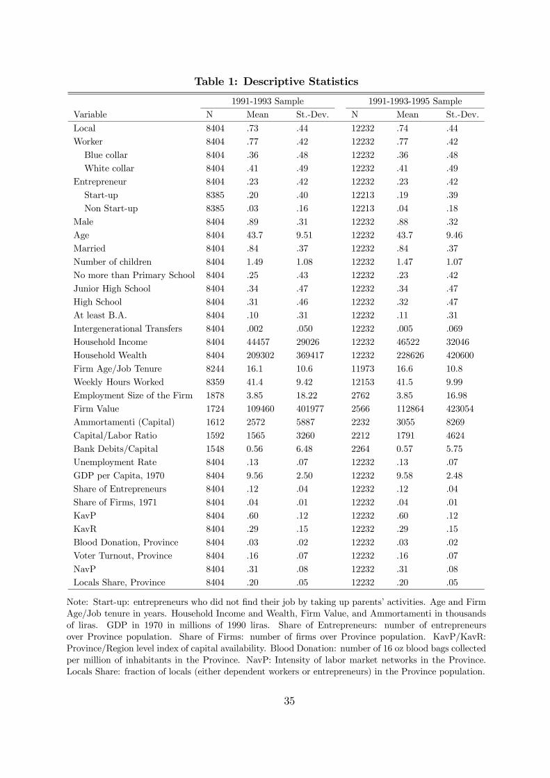
Table 1: Descriptive Statistics

1991-1993 Sample 1991-1993-1995 SampleVariable N Mean St.-Dev. N Mean St.-Dev.

Local 8404 .73 .44 12232 .74 .44Worker 8404 .77 .42 12232 .77 .42

Blue collar 8404 .36 .48 12232 .36 .48White collar 8404 .41 .49 12232 .41 .49

Entrepreneur 8404 .23 .42 12232 .23 .42

Start-up 8385 .20 .40 12213 .19 .39Non Start-up 8385 .03 .16 12213 .04 .18

Male 8404 .89 .31 12232 .88 .32Age 8404 43.7 9.51 12232 43.7 9.46Married 8404 .84 .37 12232 .84 .37

Number of children 8404 1.49 1.08 12232 1.47 1.07No more than Primary School 8404 .25 .43 12232 .23 .42

Junior High School 8404 .34 .47 12232 .34 .47High School 8404 .31 .46 12232 .32 .47At least B.A. 8404 .10 .31 12232 .11 .31

Intergenerational Transfers 8404 .002 .050 12232 .005 .069Household Income 8404 44457 29026 12232 46522 32046Household Wealth 8404 209302 369417 12232 228626 420600

Firm Age/Job Tenure 8244 16.1 10.6 11973 16.6 10.8Weekly Hours Worked 8359 41.4 9.42 12153 41.5 9.99

Employment Size of the Firm 1878 3.85 18.22 2762 3.85 16.98Firm Value 1724 109460 401977 2566 112864 423054Ammortamenti (Capital) 1612 2572 5887 2232 3055 8269

Capital/Labor Ratio 1592 1565 3260 2212 1791 4624Bank Debits/Capital 1548 0.56 6.48 2264 0.57 5.75Unemployment Rate 8404 .13 .07 12232 .13 .07

GDP per Capita, 1970 8404 9.56 2.50 12232 9.58 2.48Share of Entrepreneurs 8404 .12 .04 12232 .12 .04

Share of Firms, 1971 8404 .04 .01 12232 .04 .01KavP 8404 .60 .12 12232 .60 .12KavR 8404 .29 .15 12232 .29 .15

Blood Donation, Province 8404 .03 .02 12232 .03 .02Voter Turnout, Province 8404 .16 .07 12232 .16 .07

NavP 8404 .31 .08 12232 .31 .08Locals Share, Province 8404 .20 .05 12232 .20 .05

Note: Start-up: entrepreneurs who did not find their job by taking up parents’ activities. Age and FirmAge/Job tenure in years. Household Income and Wealth, Firm Value, and Ammortamenti in thousandsof liras. GDP in 1970 in millions of 1990 liras. Share of Entrepreneurs: number of entrepreneursover Province population. Share of Firms: number of firms over Province population. KavP/KavR:Province/Region level index of capital availability. Blood Donation: number of 16 oz blood bags collectedper million of inhabitants in the Province. NavP: Intensity of labor market networks in the Province.Locals Share: fraction of locals (either dependent workers or entrepreneurs) in the Province population.

35

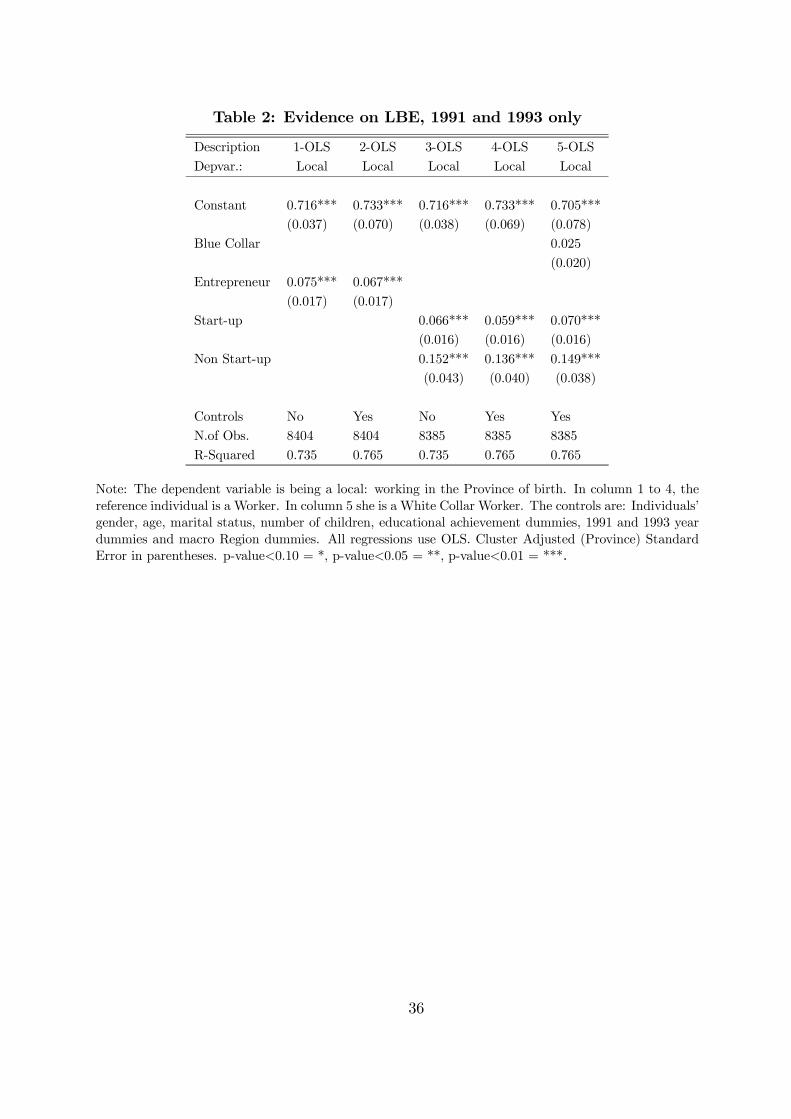
Table 2: Evidence on LBE, 1991 and 1993 only

Description 1-OLS 2-OLS 3-OLS 4-OLS 5-OLS

Depvar.: Local Local Local Local Local

Constant 0.716*** 0.733*** 0.716*** 0.733*** 0.705***(0.037) (0.070) (0.038) (0.069) (0.078)

Blue Collar 0.025

(0.020)Entrepreneur 0.075*** 0.067***

(0.017) (0.017)Start-up 0.066*** 0.059*** 0.070***

(0.016) (0.016) (0.016)

Non Start-up 0.152*** 0.136*** 0.149***(0.043) (0.040) (0.038)

Controls No Yes No Yes YesN.of Obs. 8404 8404 8385 8385 8385

R-Squared 0.735 0.765 0.735 0.765 0.765

Note: The dependent variable is being a local: working in the Province of birth. In column 1 to 4, thereference individual is a Worker. In column 5 she is a White Collar Worker. The controls are: Individuals’gender, age, marital status, number of children, educational achievement dummies, 1991 and 1993 yeardummies and macro Region dummies. All regressions use OLS. Cluster Adjusted (Province) StandardError in parentheses. p-value<0.10 = *, p-value<0.05 = **, p-value<0.01 = ***.

36

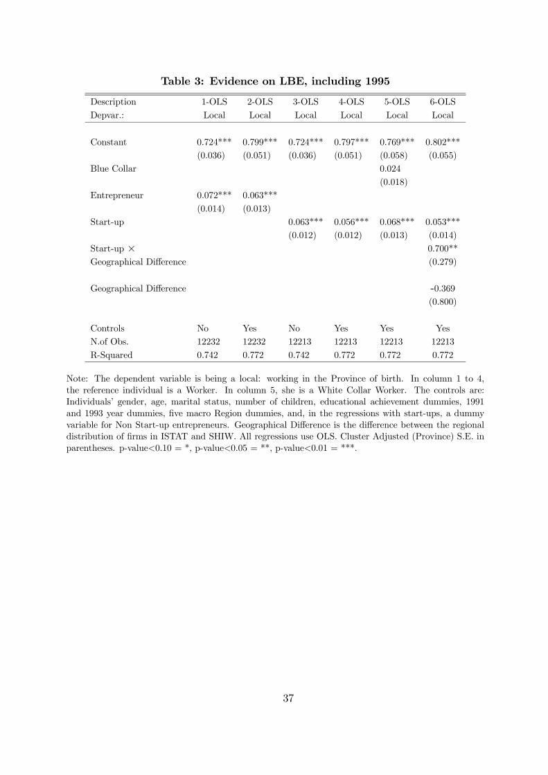
Table 3: Evidence on LBE, including 1995

Description 1-OLS 2-OLS 3-OLS 4-OLS 5-OLS 6-OLS

Depvar.: Local Local Local Local Local Local

Constant 0.724*** 0.799*** 0.724*** 0.797*** 0.769*** 0.802***(0.036) (0.051) (0.036) (0.051) (0.058) (0.055)

Blue Collar 0.024

(0.018)Entrepreneur 0.072*** 0.063***

(0.014) (0.013)Start-up 0.063*** 0.056*** 0.068*** 0.053***

(0.012) (0.012) (0.013) (0.014)

Start-up × 0.700**Geographical Difference (0.279)

Geographical Difference -0.369(0.800)

Controls No Yes No Yes Yes YesN.of Obs. 12232 12232 12213 12213 12213 12213

R-Squared 0.742 0.772 0.742 0.772 0.772 0.772

Note: The dependent variable is being a local: working in the Province of birth. In column 1 to 4,the reference individual is a Worker. In column 5, she is a White Collar Worker. The controls are:Individuals’ gender, age, marital status, number of children, educational achievement dummies, 1991and 1993 year dummies, five macro Region dummies, and, in the regressions with start-ups, a dummyvariable for Non Start-up entrepreneurs. Geographical Difference is the difference between the regionaldistribution of firms in ISTAT and SHIW. All regressions use OLS. Cluster Adjusted (Province) S.E. inparentheses. p-value<0.10 = *, p-value<0.05 = **, p-value<0.01 = ***.

37

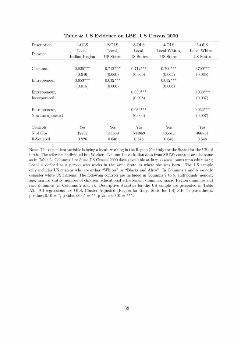
Table 4: US Evidence on LBE, US Census 2000

Description 1-OLS 2-OLS 3-OLS 4-OLS 5-OLS

Depvar.:Local,

Italian RegionLocal,

US StatesLocal,

US StatesLocal-Whites,US States

Local-Whites,US States

Constant 0.825*** 0.712*** 0.712*** 0.700*** 0.700***(0.046) (0.060) (0.060) (0.065) (0.065)

Entrepreneur 0.053*** 0.032*** 0.032***(0.015) (0.006) (0.006)

Entrepreneur, 0.030*** 0.033***Incorporated (0.008) (0.007)

Entrepreneur, 0.032*** 0.032***Non-Incorporated (0.006) (0.007)

Controls Yes Yes Yes Yes YesN.of Obs. 12232 544869 544869 486511 486511

R-Squared 0.826 0.646 0.646 0.648 0.648

Note: The dependent variable is being a local: working in the Region (for Italy) or the State (for the US) ofbirth. The reference individual is a Worker. Column 1 uses Italian data from SHIW; controls are the sameas in Table 5. Columns 2 to 5 use US Census 2000 data (available at http://www.ipums.umn.edu/usa/);Local is defined as a person who works in the same State as where she was born. The US sampleonly includes US citizens who are either “Whites” or “Blacks and Afros”. In Columns 4 and 5 we onlyconsider white US citizens. The following controls are included in Columns 2 to 5: Individuals’ gender,age, marital status, number of children, educational achievement dummies, macro Region dummies andrace dummies (in Columns 2 and 3). Descriptive statistics for the US sample are presented in TableA2. All regressions use OLS. Cluster Adjusted (Region for Italy; State for US) S.E. in parentheses.p-value<0.10 = *, p-value<0.05 = **, p-value<0.01 = ***.

38

Table 5: LBE by Firm Size

Description 1-OLS 2-OLS 3-OLS 4-OLS

Depvar.: Local Local Local Local

Panel A: Employment Size

Constant 0.724*** 0.799*** 0.724*** 0.798***(0.036) (0.051) (0.036) (0.051)

Start-up 0.044*** 0.033*** 0.056*** 0.047***(0.014) (0.014) (0.012) (0.012)

Start-up × 0.046** 0.058***Employing more than one individual (0.021) (0.018)

Start-up × 0.043* 0.059**Employing more than five individual (0.025) (0.026)

Controls No Yes No YesN.of Obs. 12177 12177 12177 12177

R-Squared 0.742 0.772 0.742 0.771

Panel B: Market Value

Constant 0.725*** 0.798*** 0.725*** 0.799***(0.036) (0.051) (0.036) (0.051)

Start-up 0.045*** 0.038** 0.056*** 0.049***

(0.015) (0.021) (0.013) (0.013)Start-up × 0.038* 0.038**Firm value greater than the median (0.023) (0.021)

Start-up × 0.046 0.052*

Firm value greater than top decile (0.034) (0.031)

Controls No Yes No Yes

N.of Obs. 11983 11983 11983 11983R-Squared 0.741 0.770 0.741 0.770

Note: The dependent variable is being a local: working in the Province of birth. The reference individualis a Worker. The controls are: Individuals’ gender, age, marital status, number of children, educationalachievement dummies, 1991 and 1993 year dummies, macro Region dummies, and a dummy variable forNon Start-up entrepreneurs. All regressions use OLS. Cluster Adjusted (Province) S.E. in parentheses.p-value<0.10 = *, p-value<0.05 = **, p-value<0.01 = ***.

39

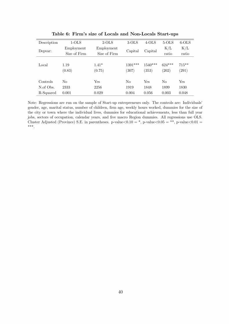
Table 6: Firm’s size of Locals and Non-Locals Start-ups

Description 1-OLS 2-OLS 3-OLS 4-OLS 5-OLS 6-OLS

Depvar:EmploymentSize of Firm

EmploymentSize of Firm

Capital CapitalK/Lratio

K/Lratio

Local 1.19 1.41* 1391*** 1540*** 624*** 715**(0.83) (0.75) (307) (353) (202) (291)

Controls No Yes No Yes No Yes

N.of Obs. 2333 2256 1919 1848 1899 1830R-Squared 0.001 0.029 0.004 0.056 0.003 0.048

Note: Regressions are run on the sample of Start-up entrepreneurs only. The controls are: Individuals’gender, age, marital status, number of children, firm age, weekly hours worked, dummies for the size ofthe city or town where the individual lives, dummies for educational achievements, less than full yearjobs, sectors of occupation, calendar years, and five macro Region dummies. All regressions use OLS.Cluster Adjusted (Province) S.E. in parentheses. p-value<0.10 = *, p-value<0.05 = **, p-value<0.01 =***.

40

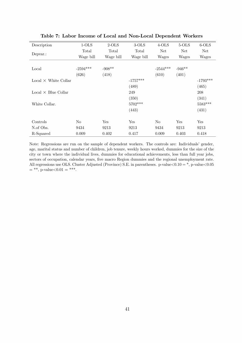
Table 7: Labor Income of Local and Non-Local Dependent Workers

Description 1-OLS 2-OLS 3-OLS 4-OLS 5-OLS 6-OLS

Depvar.:Total

Wage billTotal

Wage billTotal

Wage billNetWages

NetWages

NetWages

Local -2594*** -908** -2544*** -946**(626) (418) (610) (401)

Local × White Collar -1757*** -1793***(489) (465)

Local × Blue Collar 249 208(350) (341)

White Collar. 5702*** 5583***

(443) (431)

Controls No Yes Yes No Yes YesN.of Obs. 9434 9213 9213 9434 9213 9213R-Squared 0.009 0.402 0.417 0.009 0.403 0.418

Note: Regressions are run on the sample of dependent workers. The controls are: Individuals’ gender,age, marital status and number of children, job tenure, weekly hours worked, dummies for the size of thecity or town where the individual lives, dummies for educational achievements, less than full year jobs,sectors of occupation, calendar years, five macro Region dummies and the regional unemployment rate.All regressions use OLS. Cluster Adjusted (Province) S.E. in parentheses. p-value<0.10 = *, p-value<0.05= **, p-value<0.01 = ***.

41

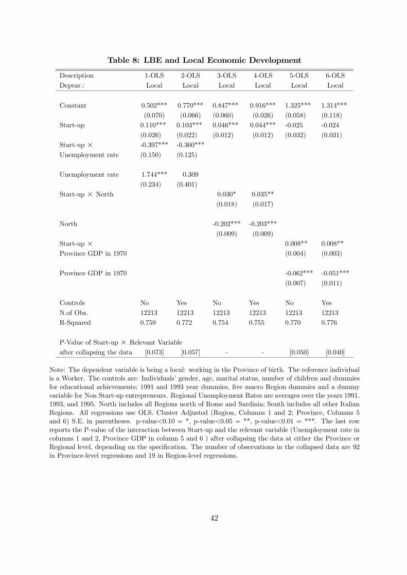
Table 8: LBE and Local Economic Development

Description 1-OLS 2-OLS 3-OLS 4-OLS 5-OLS 6-OLS

Depvar.: Local Local Local Local Local Local

Constant 0.502*** 0.770*** 0.847*** 0.916*** 1.325*** 1.314***(0.070) (0.066) (0.060) (0.026) (0.058) (0.118)

Start-up 0.110*** 0.103*** 0.046*** 0.044*** -0.025 -0.024

(0.026) (0.022) (0.012) (0.012) (0.032) (0.031)Start-up × -0.397*** -0.360***

Unemployment rate (0.150) (0.125)

Unemployment rate 1.744*** 0.309

(0.234) (0.401)Start-up × North 0.030* 0.035**

(0.018) (0.017)

North -0.202*** -0.203***

(0.009) (0.009)Start-up × 0.008** 0.008**Province GDP in 1970 (0.004) (0.003)

Province GDP in 1970 -0.062*** -0.051***

(0.007) (0.011)

Controls No Yes No Yes No Yes

N.of Obs. 12213 12213 12213 12213 12213 12213R-Squared 0.759 0.772 0.754 0.755 0.770 0.776

P-Value of Start-up × Relevant Variableafter collapsing the data [0.073] [0.057] - - [0.050] [0.040]

Note: The dependent variable is being a local: working in the Province of birth. The reference individualis a Worker. The controls are: Individuals’ gender, age, marital status, number of children and dummiesfor educational achievements; 1991 and 1993 year dummies, five macro Region dummies and a dummyvariable for Non Start-up entrepreneurs. Regional Unemployment Rates are averages over the years 1991,1993, and 1995. North includes all Regions north of Rome and Sardinia; South includes all other ItalianRegions. All regressions use OLS. Cluster Adjusted (Region, Columns 1 and 2; Province, Columns 5and 6) S.E. in parentheses. p-value<0.10 = *, p-value<0.05 = **, p-value<0.01 = ***. The last rowreports the P-value of the interaction between Start-up and the relevant variable (Unemployment rate incolumns 1 and 2, Province GDP in column 5 and 6 ) after collapsing the data at either the Province orRegional level, depending on the specification. The number of observations in the collapsed data are 92in Province-level regressions and 19 in Region-level regressions.

42

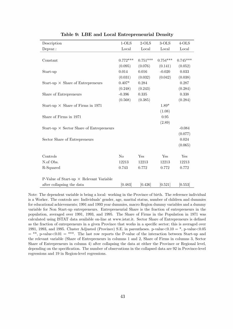
Table 9: LBE and Local Entrepreneurial Density

Description 1-OLS 2-OLS 3-OLS 4-OLS

Depvar.: Local Local Local Local

Constant 0.772*** 0.751*** 0.754*** 0.745***(0.095) (0.076) (0.141) (0.052)

Start-up 0.014 0.016 -0.020 0.033

(0.031) (0.032) (0.042) (0.038)Start-up × Share of Entrepreneurs 0.407* 0.284 0.287

(0.248) (0.243) (0.284)Share of Entrepreneurs -0.396 0.335 0.338

(0.568) (0.385) (0.284)

Start-up × Share of Firms in 1971 1.89*(1.08)

Share of Firms in 1971 0.95(2.89)

Start-up × Sector Share of Entrepreneurs -0.084

(0.077)Sector Share of Entrepreneurs 0.024

(0.065)

Controls No Yes Yes Yes

N.of Obs. 12213 12213 12213 12213R-Squared 0.743 0.772 0.772 0.772

P-Value of Start-up × Relevant Variableafter collapsing the data [0.483] [0.426] [0.521] [0.553]

Note: The dependent variable is being a local: working in the Province of birth. The reference individualis a Worker. The controls are: Individuals’ gender, age, marital status, number of children and dummiesfor educational achievements; 1991 and 1993 year dummies, macro Region dummy variables and a dummyvariable for Non Start-up entrepreneurs. Entrepreneurial Share is the fraction of entrepreneurs in thepopulation, averaged over 1991, 1993, and 1995. The Share of Firms in the Population in 1971 wascalculated using ISTAT data available on-line at www.istat.it. Sector Share of Entrepreneurs is definedas the fraction of entrepreneurs in a given Province that works in a specific sector; this is averaged over1991, 1993, and 1995. Cluster Adjusted (Province) S.E. in parentheses. p-value<0.10 = *, p-value<0.05= **, p-value<0.01 = ***. The last row reports the P-value of the interaction between Start-up andthe relevant variable (Share of Entrepreneurs in columns 1 and 2, Share of Firms in columns 3, SectorShare of Entrepreneurs in column 4) after collapsing the data at either the Province or Regional level,depending on the specification. The number of observations in the collapsed data are 92 in Province-levelregressions and 19 in Region-level regressions.

43

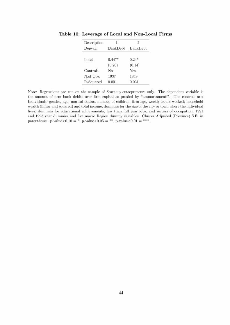
Table 10: Leverage of Local and Non-Local Firms

Description 1 2

Depvar: BankDebt BankDebt

Local 0.44** 0.24*(0.20) (0.14)

Controls No Yes

N.of Obs. 1937 1849R-Squared 0.001 0.031

Note: Regressions are run on the sample of Start-up entrepreneurs only. The dependent variable isthe amount of firm bank debits over firm capital as proxied by “ammortamenti”. The controls are:Individuals’ gender, age, marital status, number of children, firm age, weekly hours worked; householdwealth (linear and squared) and total income; dummies for the size of the city or town where the individuallives; dummies for educational achievements, less than full year jobs, and sectors of occupation; 1991and 1993 year dummies and five macro Region dummy variables. Cluster Adjusted (Province) S.E. inparentheses. p-value<0.10 = *, p-value<0.05 = **, p-value<0.01 = ***.

44

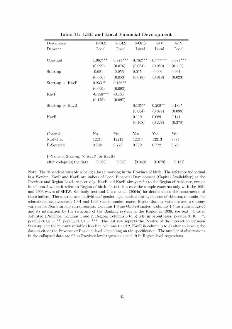
Table 11: LBE and Local Financial Development

Description 1-OLS 2-OLS 3-OLS 4-IV 5-IV

Depvar.: Local Local Local Local Local

Constant 1.062*** 0.877*** 0.762*** 0.777*** 0.687***(0.099) (0.076) (0.064) (0.080) (0.117)

Start-up -0.081 -0.056 0.015 -0.006 0.001

(0.056) (0.053) (0.018) (0.019) (0.023)Start-up × KavP 0.233** 0.186**

(0.099) (0.093)KavP -0.558*** -0.135

(0.175) (0.097)

Start-up × KavR 0.135** 0.209** 0.189*(0.064) (0.077) (0.098)

KavR 0.119 0.069 0.141(0.168) (0.228) (0.278)

Controls No Yes Yes Yes YesN.of Obs. 12213 12213 12213 12213 8385R-Squared 0.748 0.772 0.772 0.772 0.765

P-Value of Start-up × KavP (or KavR)

after collapsing the data [0.089] [0.083] [0.049] [0.079] [0.167]

Note: The dependent variable is being a local: working in the Province of birth. The reference individualis a Worker. KavP and KavR are indices of Local Financial Development (Capital Availability) at theProvince and Region Level, respectively. KavP and KavR always refer to the Region of residence, exceptin column 5 where it refers to Region of birth. In this last case the sample concerns only with the 1991and 1993 waves of SHIW. See body text and Guiso at al. (2004a) for details about the construction ofthese indices. The controls are: Individuals’ gender, age, marital status, number of children, dummies foreducational achievements, 1991 and 1993 year dummies, macro Region dummy variables and a dummyvariable for Non Start-up entrepreneurs. Columns 1-3 are OLS estimates. Columns 4-5 instrument KavRand its interaction by the structure of the Banking system in the Region in 1936, see text. ClusterAdjusted (Province, Columns 1 and 2; Region, Columns 3 to 5) S.E. in parentheses. p-value<0.10 = *,p-value<0.05 = **, p-value<0.01 = ***. The last row reports the P-value of the interaction betweenStart-up and the relevant variable (KavP in columns 1 and 2, KavR in column 3 to 5) after collapsing thedata at either the Province or Regional level, depending on the specification. The number of observationsin the collapsed data are 92 in Province-level regressions and 19 in Region-level regressions.

45

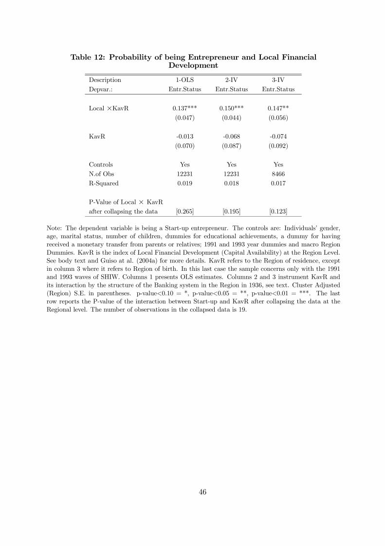
Table 12: Probability of being Entrepreneur and Local FinancialDevelopment

Description 1-OLS 2-IV 3-IV

Depvar.: Entr.Status Entr.Status Entr.Status

Local ×KavR 0.137*** 0.150*** 0.147**

(0.047) (0.044) (0.056)

KavR -0.013 -0.068 -0.074

(0.070) (0.087) (0.092)

Controls Yes Yes Yes

N.of Obs 12231 12231 8466R-Squared 0.019 0.018 0.017

P-Value of Local × KavRafter collapsing the data [0.265] [0.195] [0.123]

Note: The dependent variable is being a Start-up entrepreneur. The controls are: Individuals’ gender,age, marital status, number of children, dummies for educational achievements, a dummy for havingreceived a monetary transfer from parents or relatives; 1991 and 1993 year dummies and macro RegionDummies. KavR is the index of Local Financial Development (Capital Availability) at the Region Level.See body text and Guiso at al. (2004a) for more details. KavR refers to the Region of residence, exceptin column 3 where it refers to Region of birth. In this last case the sample concerns only with the 1991and 1993 waves of SHIW. Columns 1 presents OLS estimates. Columns 2 and 3 instrument KavR andits interaction by the structure of the Banking system in the Region in 1936, see text. Cluster Adjusted(Region) S.E. in parentheses. p-value<0.10 = *, p-value<0.05 = **, p-value<0.01 = ***. The lastrow reports the P-value of the interaction between Start-up and KavR after collapsing the data at theRegional level. The number of observations in the collapsed data is 19.

46

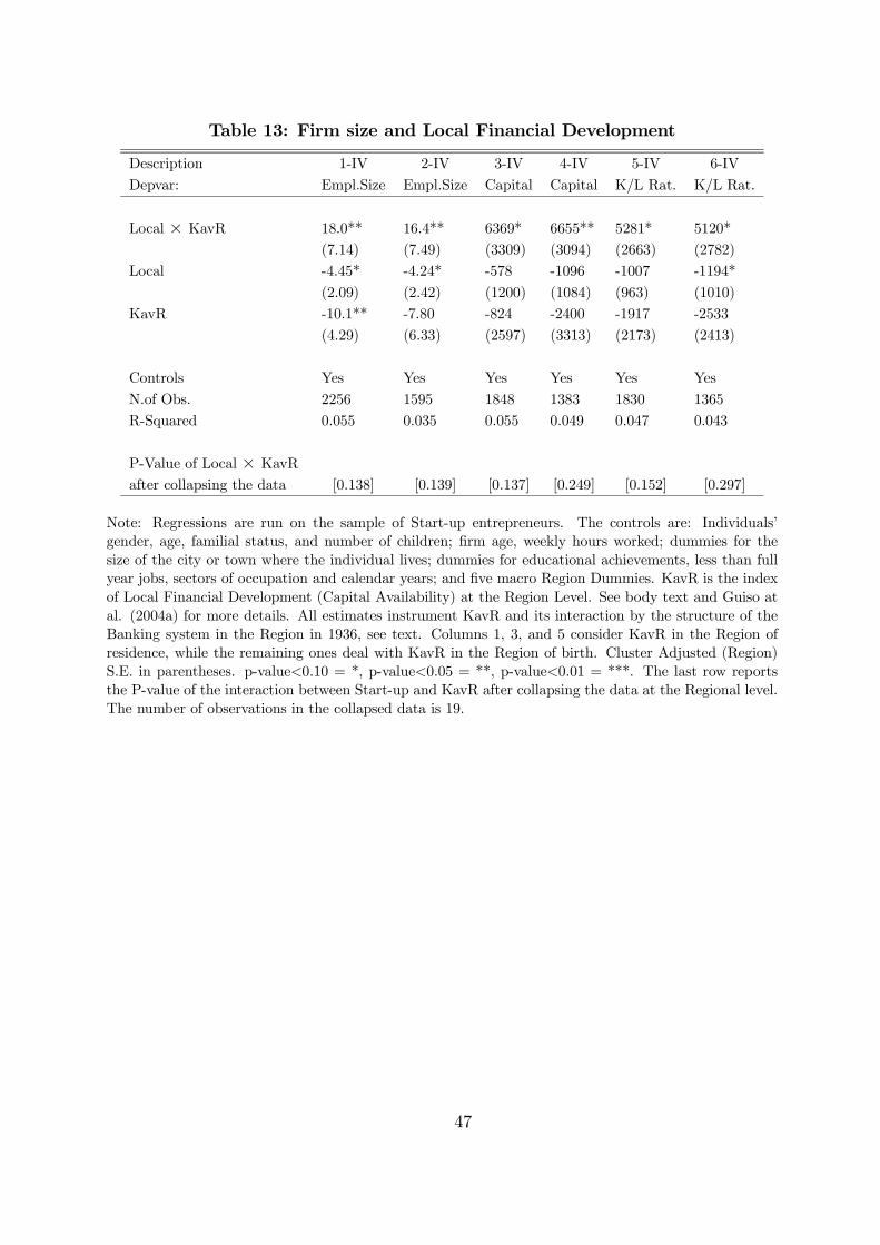
Table 13: Firm size and Local Financial Development

Description 1-IV 2-IV 3-IV 4-IV 5-IV 6-IV

Depvar: Empl.Size Empl.Size Capital Capital K/L Rat. K/L Rat.

Local × KavR 18.0** 16.4** 6369* 6655** 5281* 5120*(7.14) (7.49) (3309) (3094) (2663) (2782)

Local -4.45* -4.24* -578 -1096 -1007 -1194*

(2.09) (2.42) (1200) (1084) (963) (1010)KavR -10.1** -7.80 -824 -2400 -1917 -2533

(4.29) (6.33) (2597) (3313) (2173) (2413)

Controls Yes Yes Yes Yes Yes Yes

N.of Obs. 2256 1595 1848 1383 1830 1365R-Squared 0.055 0.035 0.055 0.049 0.047 0.043

P-Value of Local × KavRafter collapsing the data [0.138] [0.139] [0.137] [0.249] [0.152] [0.297]

Note: Regressions are run on the sample of Start-up entrepreneurs. The controls are: Individuals’gender, age, familial status, and number of children; firm age, weekly hours worked; dummies for thesize of the city or town where the individual lives; dummies for educational achievements, less than fullyear jobs, sectors of occupation and calendar years; and five macro Region Dummies. KavR is the indexof Local Financial Development (Capital Availability) at the Region Level. See body text and Guiso atal. (2004a) for more details. All estimates instrument KavR and its interaction by the structure of theBanking system in the Region in 1936, see text. Columns 1, 3, and 5 consider KavR in the Region ofresidence, while the remaining ones deal with KavR in the Region of birth. Cluster Adjusted (Region)S.E. in parentheses. p-value<0.10 = *, p-value<0.05 = **, p-value<0.01 = ***. The last row reportsthe P-value of the interaction between Start-up and KavR after collapsing the data at the Regional level.The number of observations in the collapsed data is 19.

47

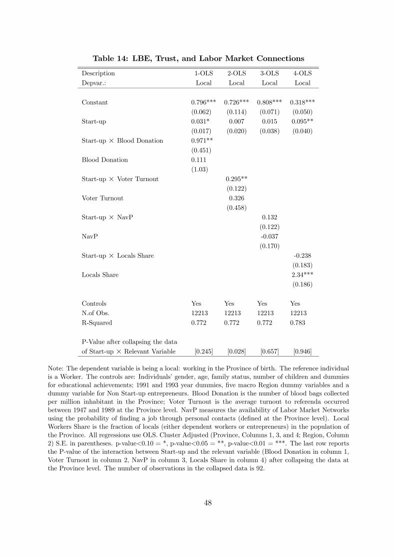
Table 14: LBE, Trust, and Labor Market Connections

Description 1-OLS 2-OLS 3-OLS 4-OLS

Depvar.: Local Local Local Local

Constant 0.796*** 0.726*** 0.808*** 0.318***(0.062) (0.114) (0.071) (0.050)

Start-up 0.031* 0.007 0.015 0.095**

(0.017) (0.020) (0.038) (0.040)Start-up × Blood Donation 0.971**

(0.451)Blood Donation 0.111

(1.03)

Start-up × Voter Turnout 0.295**(0.122)

Voter Turnout 0.326(0.458)

Start-up × NavP 0.132

(0.122)NavP -0.037

(0.170)

Start-up × Locals Share -0.238(0.183)

Locals Share 2.34***(0.186)

Controls Yes Yes Yes YesN.of Obs. 12213 12213 12213 12213

R-Squared 0.772 0.772 0.772 0.783

P-Value after collapsing the data

of Start-up × Relevant Variable [0.245] [0.028] [0.657] [0.946]

Note: The dependent variable is being a local: working in the Province of birth. The reference individualis a Worker. The controls are: Individuals’ gender, age, family status, number of children and dummiesfor educational achievements; 1991 and 1993 year dummies, five macro Region dummy variables and adummy variable for Non Start-up entrepreneurs. Blood Donation is the number of blood bags collectedper million inhabitant in the Province; Voter Turnout is the average turnout to referenda occurredbetween 1947 and 1989 at the Province level. NavP measures the availability of Labor Market Networksusing the probability of finding a job through personal contacts (defined at the Province level). LocalWorkers Share is the fraction of locals (either dependent workers or entrepreneurs) in the population ofthe Province. All regressions use OLS. Cluster Adjusted (Province, Columns 1, 3, and 4; Region, Column2) S.E. in parentheses. p-value<0.10 = *, p-value<0.05 = **, p-value<0.01 = ***. The last row reportsthe P-value of the interaction between Start-up and the relevant variable (Blood Donation in column 1,Voter Turnout in column 2, NavP in column 3, Locals Share in column 4) after collapsing the data atthe Province level. The number of observations in the collapsed data is 92.

48

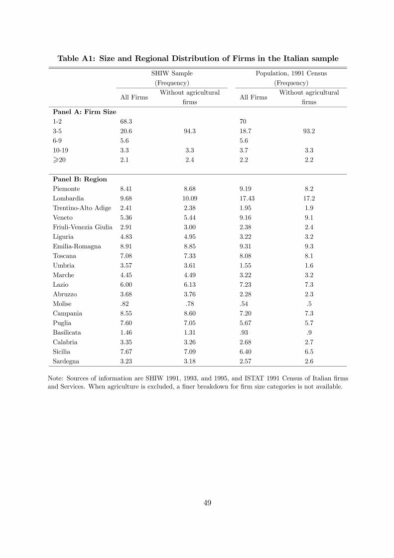
Table A1: Size and Regional Distribution of Firms in the Italian sample

SHIW Sample

(Frequency)

Population, 1991 Census

(Frequency)

All FirmsWithout agricultural

firmsAll Firms

Without agriculturalfirms

Panel A: Firm Size1-2 68.3 70

3-5 20.6 94.3 18.7 93.26-9 5.6 5.6

10-19 3.3 3.3 3.7 3.3>20 2.1 2.4 2.2 2.2

Panel B: RegionPiemonte 8.41 8.68 9.19 8.2

Lombardia 9.68 10.09 17.43 17.2Trentino-Alto Adige 2.41 2.38 1.95 1.9

Veneto 5.36 5.44 9.16 9.1Friuli-Venezia Giulia 2.91 3.00 2.38 2.4Liguria 4.83 4.95 3.22 3.2

Emilia-Romagna 8.91 8.85 9.31 9.3Toscana 7.08 7.33 8.08 8.1

Umbria 3.57 3.61 1.55 1.6Marche 4.45 4.49 3.22 3.2Lazio 6.00 6.13 7.23 7.3

Abruzzo 3.68 3.76 2.28 2.3Molise .82 .78 .54 .5Campania 8.55 8.60 7.20 7.3

Puglia 7.60 7.05 5.67 5.7Basilicata 1.46 1.31 .93 .9

Calabria 3.35 3.26 2.68 2.7Sicilia 7.67 7.09 6.40 6.5Sardegna 3.23 3.18 2.57 2.6

Note: Sources of information are SHIW 1991, 1993, and 1995, and ISTAT 1991 Census of Italian firmsand Services. When agriculture is excluded, a finer breakdown for firm size categories is not available.

49

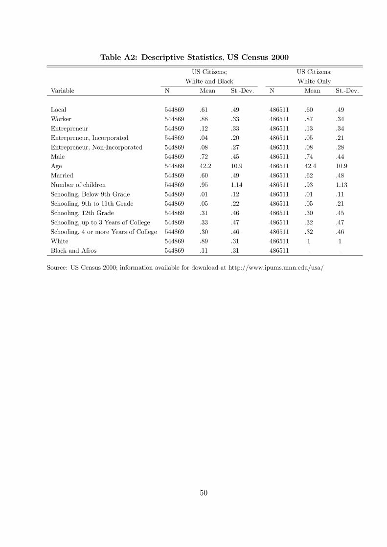
Table A2: Descriptive Statistics, US Census 2000

US Citizens;

White and Black

US Citizens;

White OnlyVariable N Mean St.-Dev. N Mean St.-Dev.

Local 544869 .61 .49 486511 .60 .49Worker 544869 .88 .33 486511 .87 .34

Entrepreneur 544869 .12 .33 486511 .13 .34Entrepreneur, Incorporated 544869 .04 .20 486511 .05 .21

Entrepreneur, Non-Incorporated 544869 .08 .27 486511 .08 .28Male 544869 .72 .45 486511 .74 .44Age 544869 42.2 10.9 486511 42.4 10.9

Married 544869 .60 .49 486511 .62 .48Number of children 544869 .95 1.14 486511 .93 1.13

Schooling, Below 9th Grade 544869 .01 .12 486511 .01 .11Schooling, 9th to 11th Grade 544869 .05 .22 486511 .05 .21Schooling, 12th Grade 544869 .31 .46 486511 .30 .45

Schooling, up to 3 Years of College 544869 .33 .47 486511 .32 .47Schooling, 4 or more Years of College 544869 .30 .46 486511 .32 .46White 544869 .89 .31 486511 1 1

Black and Afros 544869 .11 .31 486511 — —

Source: US Census 2000; information available for download at http://www.ipums.umn.edu/usa/

50