1 | P a g e

WHY QUANTITATIVE EASING CAN NEVER WORK

The term quantitative easing (QE) is not a random assemblage of words. Both were chosen specifically to convey specific meaning and intention. The first, quantitative, was chosen to signify the sound scientific principles of monetary economics by econometrics, the statistical study of money and economy. It signifies that the central bank implementing QE has measured and quantified both the monetary shortfall and the precise quantity needed to correct it. The second part of the phrase, easing, is the expected result of the quantity action described. The modern central bank functions through open market operations of security transactions with its dealer networks. Therefore, “easing” is increasing the level of bank reserves. Prior to the global financial crisis, starting in August 2007, the idea of monetary policy “easing” was accomplished implicitly by targeting a specific money interest rate. The central bank declared a lower rate target and the private banking system dutifully created whatever “money” needed to accomplish “easing.” That stands as the bright, significant dividing line between the pre-crisis era and the monetary history following it (so far). Understanding (belatedly) the nature of the crisis, central banks were forced into an explicit easing, directly affecting the level of bank reserves. When implicit methods proved disastrously insufficient, “extraordinary” monetary policies – QE – were implemented. Thus, the three pronged nature of QE principles: 1. When the private market for money is impaired implicit central bank “easing” must become explicit central bank balance sheet expansion; 2. Although the explicit method is still open market operations, the end result of “easing” is a determined increase in the level of bank reserves which are taken for “money”; 3. The Federal Reserve and/or any other central bank practicing QE knows the quantity of bank reserves which will accomplish its goals.

2 | P a g e

The very fact that there was a QE2 undermines at least the third principle. A second program signifies that the quantity calculation of the first was wrong or incomplete. The addition of a third round (MBS, October 2012) and then a fourth (UST, December 2012) only further demonstrates that there are inherent flaws. The question is whether those flaws extend beyond finding the right quantity. The economy in 2016 is shakier now than at any point since the Great Recession. There is an inarguable manufacturing recession in the United States but also spread across the globe and trade is down significantly. None of the major economies that have undertaken QE can show definitive evidence of its efficacy, always seeming to need more. Not only are there serious questions about growth in each but inflation is curiously absent and getting more so all the time despite radical balance sheet expansion. The response to this failure in Europe and Japan has been to do more QE, to further increase the “Q.” Official Federal Reserve policy has been to deny that there are any economic doubts at all, admitting only some kind of “transitory” deficiency. There are those who see beyond the Fed’s jawboning and call for more “easing.” Among them is Credit Suisse’s Zoltan Poszar who has proved himself time and again to be much more than the typical economist. Unlike orthodox economics that simply assumes a bland, blanket monetary agency, Poszar has undertaken a number of efforts to actually understand the nuance and nature of the modern, global monetary system. For him to declare another $1 trillion or more in additional bank reserves to resolve these questions is far different than a central banker just picking another number for “Q”. You can and should read his reasoning on his website, but in the interest of this discussion I will provide only a brief summary. There have been a number of changes to the financial system that have essentially caused an increase in the demand for dollars, specifically bank reserves. Among them are Basel III regulations, the LCR, as well as negative nominal rates in Europe and now Japan. The resulting combination is that global economic participants have greater incentive to hold dollar assets leading their banks to fund them by holding greater dollar reserves. The net result is this “rising dollar” that is a further impediment to the global economy. If he is correct about dollar demand, then the solution is for the Fed to supply more dollars by increasing the level of bank reserves through more balance sheet expansion (QE). Again, the fact that Mr. Poszar is calling for such action is far different in my view than practically any other mainstream economist or policymaker. Understanding the “plumbing” of the financial and monetary system as he does makes his determination immediately credible in a way that mainstream declarations do not. While working for the United States Treasury’s Office of Financial Research in July 2014, Mr. Pozsar authored one of the most remarkable reports I have ever seen. He attempted to map out the tangled and often impenetrable inner workings of the financial system. Doing so, he indelibly put to rest any notion of money and banking as simple variables devoid of inherent granularity (as if the 2008 panic weren’t enough on that count). The 67 pages of notes and commentary

3 | P a g e

accompanying the 160 pages of ledgers and financial cartography are remarkable and astounding. His description, no doubt fascinating and more accurate than anything produced before or since, was incomplete. This is not a criticism of Mr. Pozsar, rather it is recognition of the strict limitations under which we all must strain. The global financial system under the eurodollar standard cannot be measured or even seen; there is at the very least a divide between the domestic side and the vast operations, in dollars, that occur offshore far beyond our grasp. His utterly beautiful and very meaningful contribution did not - could not - overcome that further dimension. While his praiseworthy effort did a great deal to advance our understanding of the complex wholesale system, it did not address the onshore/offshore divide when coming to terms with the real world financial system; including any further call for more “Q.” The idea that another $1 trillion or any other number of additional bank reserves will be “enough” springs from this obscured viewpoint. There are, therefore, two general faults in the analysis. First is that it does not address why the private market for money has not responded to greater demand for dollars by supplying them in a fashion equivalent and substitutable to bank reserves. The second flaw is related to the first, in that it is highly likely that the “supply” of dollars is and has been greatly affected especially in those areas of the offshore dollar capacity beyond simple understanding let alone quantification. In short, QE fails on both terms as it is neither “quantitative” nor, on its own, “easing.” We have to account for the fact that because of the further complexity of modern eurodollar/wholesale money, the problem is not necessarily the quantity of bank reserves but really the exclusive emphasis upon reserves as an actionable substitute for the full range of eurodollar function and behavior. The rest of this work will follow along these lines: first to address the quantitative aspects of eurodollar finance that can be measured to put dollar QE into some meaningful (hopefully) context; second, to examine the qualitative expansion of the eurodollar system with a view to generally describing why bank reserves were not appropriate nor can they ever be; finally, to engage a short but meaningful presentation on the implications of not just the past deficiencies with respect to QE but also the dangers of continuing to deny them. SECTION 1: QUANTITATIVE CONTRACTION Taken in isolation, the Federal Reserve’s balance sheet expansion is remarkable. To its critics, especially in its earliest days, it presented a terrifying prospect of hyperinflationary possibilities. The idea of the US central bank “printing” trillions in new “money” was abhorrent to the principles of a sound dollar. But as Mr. Pozsar and many others have pointed out, the Federal Reserve had given itself the task of absorbing much of the function of the private money dealing system. There is, of course, debate as to whether it should have ever made such an attempt in

4 | P a g e

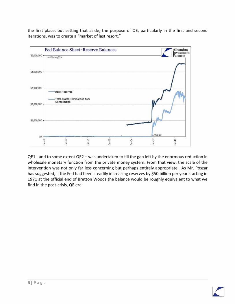
the first place, but setting that aside, the purpose of QE, particularly in the first and second iterations, was to create a “market of last resort.”

QE1 - and to some extent QE2 – was undertaken to fill the gap left by the enormous reduction in wholesale monetary function from the private money system. From that view, the scale of the intervention was not only far less concerning but perhaps entirely appropriate. As Mr. Poszar has suggested, if the Fed had been steadily increasing reserves by $50 billion per year starting in 1971 at the official end of Bretton Woods the balance would be roughly equivalent to what we find in the post-crisis, QE era.

5 | P a g e

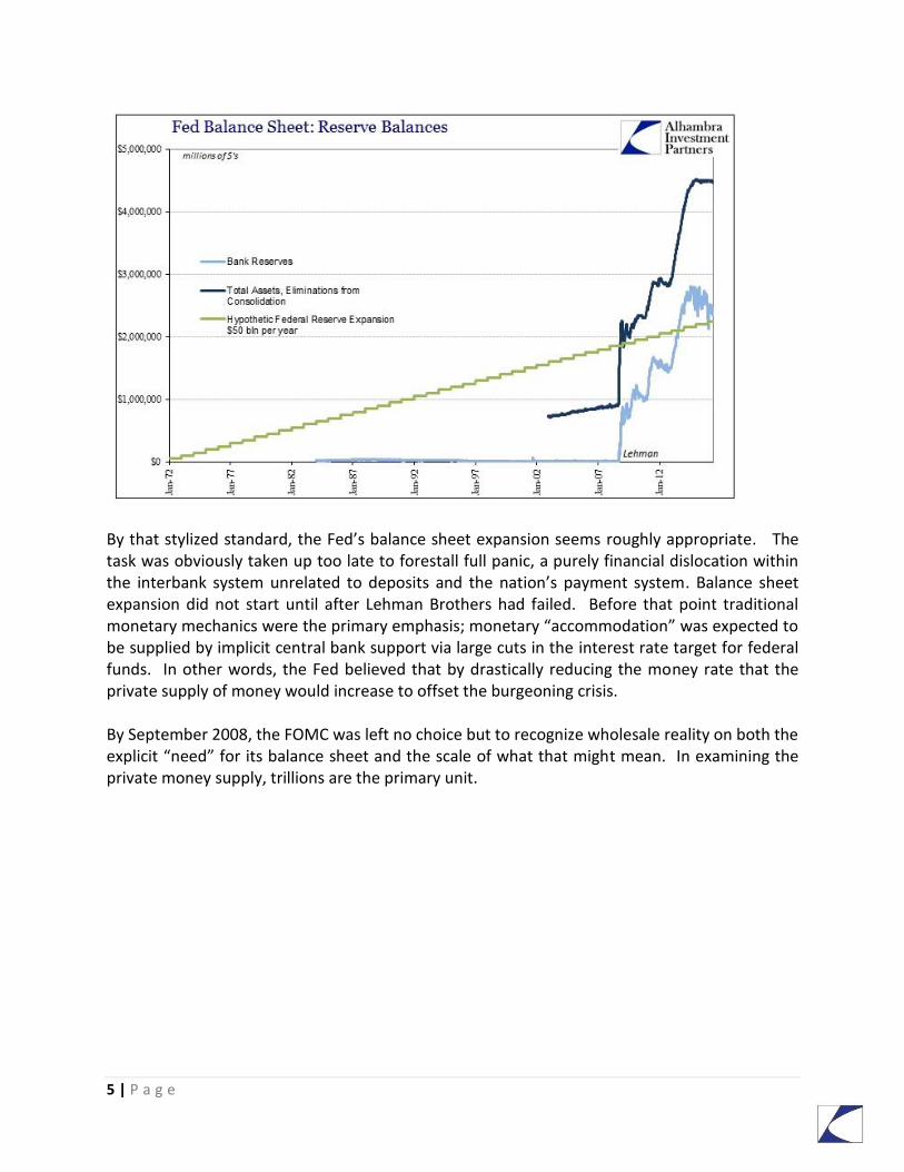
By that stylized standard, the Fed’s balance sheet expansion seems roughly appropriate. The task was obviously taken up too late to forestall full panic, a purely financial dislocation within the interbank system unrelated to deposits and the nation’s payment system. Balance sheet expansion did not start until after Lehman Brothers had failed. Before that point traditional monetary mechanics were the primary emphasis; monetary “accommodation” was expected to be supplied by implicit central bank support via large cuts in the interest rate target for federal funds. In other words, the Fed believed that by drastically reducing the money rate that the private supply of money would increase to offset the burgeoning crisis. By September 2008, the FOMC was left no choice but to recognize wholesale reality on both the explicit “need” for its balance sheet and the scale of what that might mean. In examining the private money supply, trillions are the primary unit.

6 | P a g e

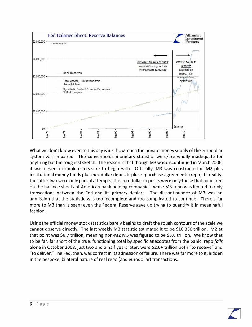
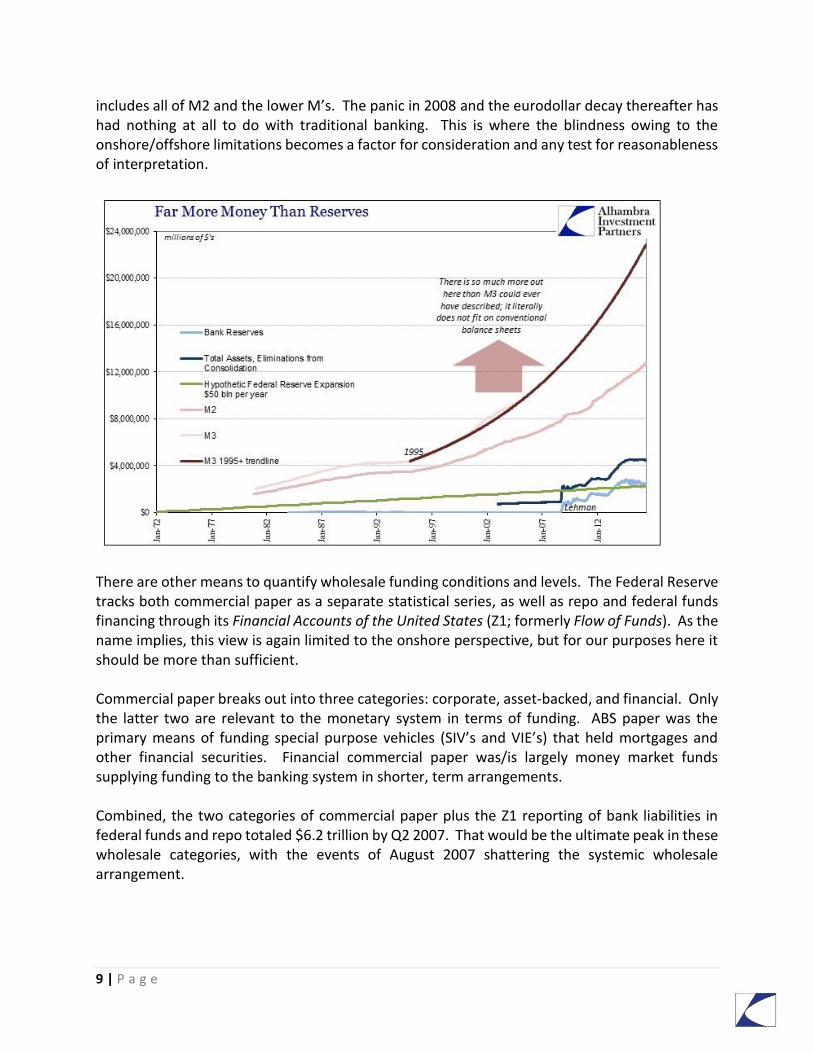
What we don’t know even to this day is just how much the private money supply of the eurodollar system was impaired. The conventional monetary statistics were/are wholly inadequate for anything but the roughest sketch. The reason is that though M3 was discontinued in March 2006, it was never a complete measure to begin with. Officially, M3 was constructed of M2 plus institutional money funds plus eurodollar deposits plus repurchase agreements (repo). In reality, the latter two were only partial attempts; the eurodollar deposits were only those that appeared on the balance sheets of American bank holding companies, while M3 repo was limited to only transactions between the Fed and its primary dealers. The discontinuance of M3 was an admission that the statistic was too incomplete and too complicated to continue. There’s far more to M3 than is seen; even the Federal Reserve gave up trying to quantify it in meaningful fashion. Using the official money stock statistics barely begins to draft the rough contours of the scale we cannot observe directly. The last weekly M3 statistic estimated it to be $10.336 trillion. M2 at that point was $6.7 trillion, meaning non-M2 M3 was figured to be $3.6 trillion. We know that to be far, far short of the true, functioning total by specific anecdotes from the panic: repo fails alone in October 2008, just two and a half years later, were $2.6+ trillion both “to receive” and “to deliver.” The Fed, then, was correct in its admission of failure. There was far more to it, hidden in the bespoke, bilateral nature of real repo (and eurodollar) transactions.

7 | P a g e

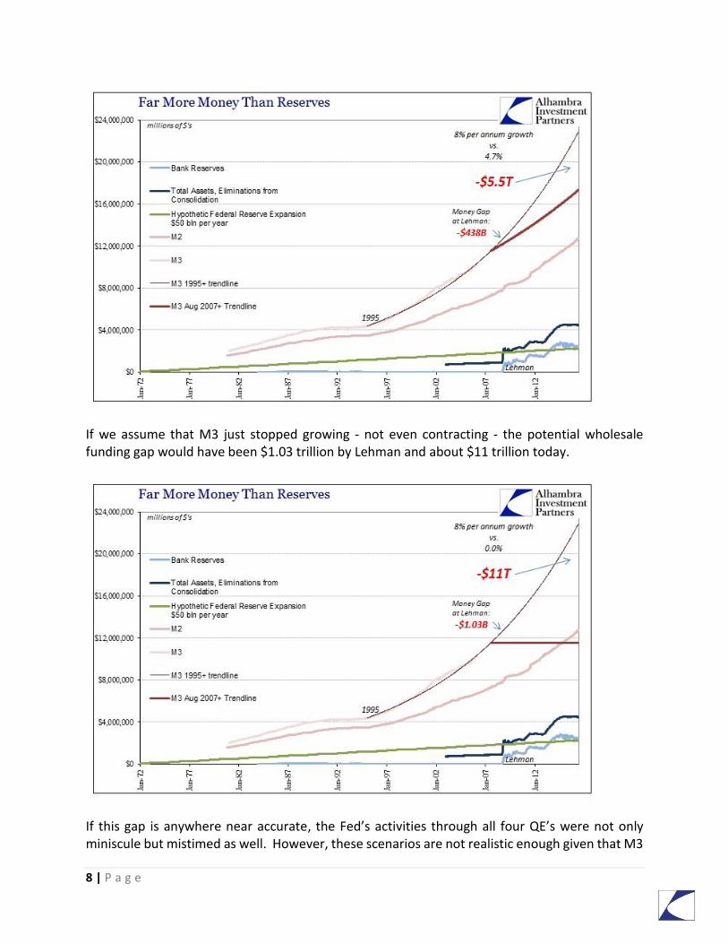
Establishing, then, M3 as just the starting point for measuring monetary policy intervention, we turn our attention to what might have happened during the crisis as it relates quantitatively to how the Federal Reserve responded. If we assume that M3 continued to grow at its baseline average, by August 9, 2007, it would have been around $11.5 trillion. That date is important as it marks the definitive break between the pre-crisis wholesale era and the dysfunction thereafter. Starting in early August 2007, if the growth rate had suddenly slowed from the 8% baseline to around 4.7%, the gap between normal operation and this hypothetical would have been $438 billion by the time of Lehman, and around $5.5 trillion today.

8 | P a g e

If we assume that M3 just stopped growing - not even contracting - the potential wholesale funding gap would have been $1.03 trillion by Lehman and about $11 trillion today.

If this gap is anywhere near accurate, the Fed’s activities through all four QE’s were not only miniscule but mistimed as well. However, these scenarios are not realistic enough given that M3

9 | P a g e

includes all of M2 and the lower M’s. The panic in 2008 and the eurodollar decay thereafter has had nothing at all to do with traditional banking. This is where the blindness owing to the onshore/offshore limitations becomes a factor for consideration and any test for reasonableness of interpretation.

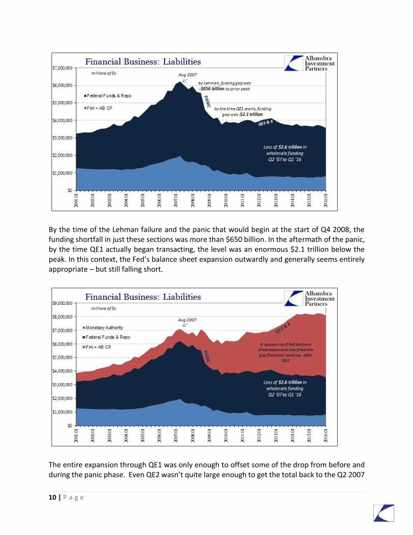
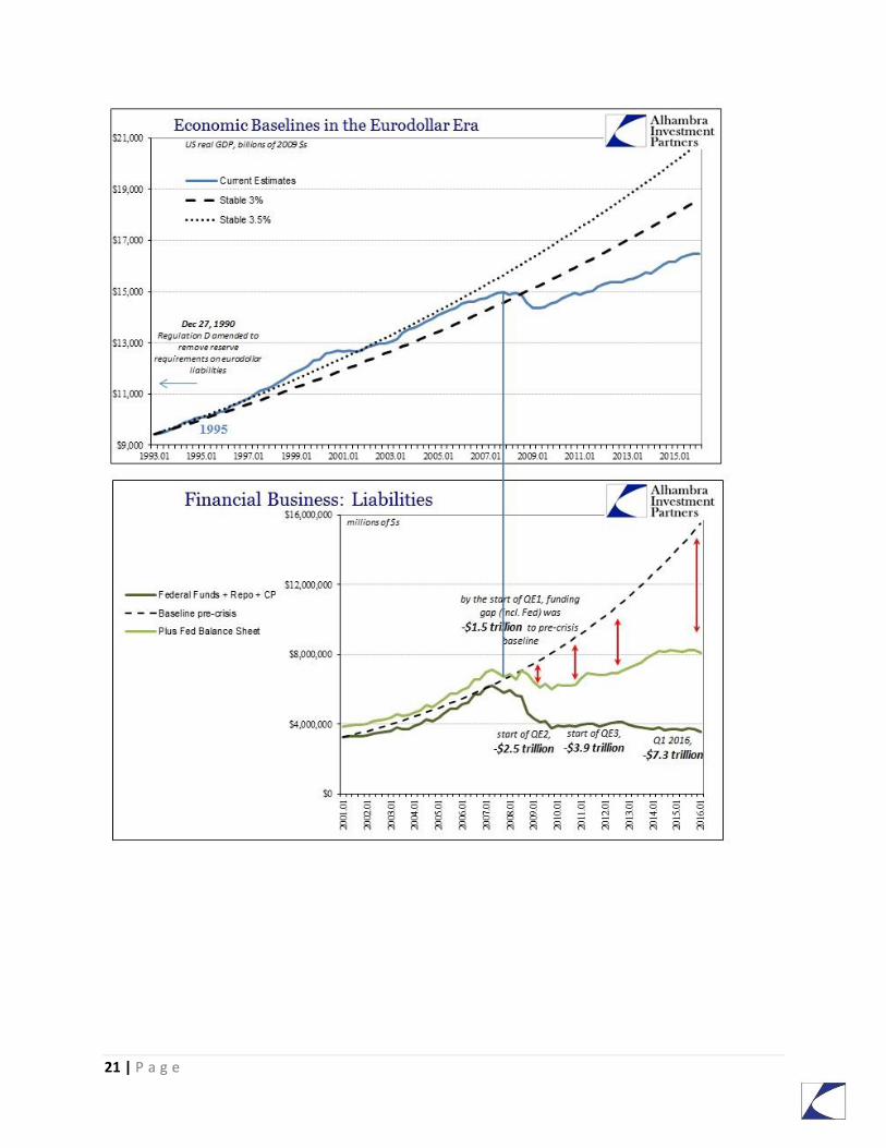
There are other means to quantify wholesale funding conditions and levels. The Federal Reserve tracks both commercial paper as a separate statistical series, as well as repo and federal funds financing through its Financial Accounts of the United States (Z1; formerly Flow of Funds). As the name implies, this view is again limited to the onshore perspective, but for our purposes here it should be more than sufficient. Commercial paper breaks out into three categories: corporate, asset-backed, and financial. Only the latter two are relevant to the monetary system in terms of funding. ABS paper was the primary means of funding special purpose vehicles (SIV’s and VIE’s) that held mortgages and other financial securities. Financial commercial paper was/is largely money market funds supplying funding to the banking system in shorter, term arrangements. Combined, the two categories of commercial paper plus the Z1 reporting of bank liabilities in federal funds and repo totaled $6.2 trillion by Q2 2007. That would be the ultimate peak in these wholesale categories, with the events of August 2007 shattering the systemic wholesale arrangement.

10 | P a g e

By the time of the Lehman failure and the panic that would begin at the start of Q4 2008, the funding shortfall in just these sections was more than $650 billion. In the aftermath of the panic, by the time QE1 actually began transacting, the level was an enormous $2.1 trillion below the peak. In this context, the Fed’s balance sheet expansion outwardly and generally seems entirely appropriate – but still falling short.

The entire expansion through QE1 was only enough to offset some of the drop from before and during the panic phase. Even QE2 wasn’t quite large enough to get the total back to the Q2 2007

11 | P a g e

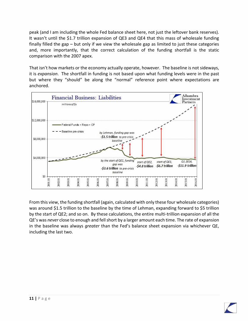
peak (and I am including the whole Fed balance sheet here, not just the leftover bank reserves). It wasn’t until the $1.7 trillion expansion of QE3 and QE4 that this mass of wholesale funding finally filled the gap – but only if we view the wholesale gap as limited to just these categories and, more importantly, that the correct calculation of the funding shortfall is the static comparison with the 2007 apex. That isn’t how markets or the economy actually operate, however. The baseline is not sideways, it is expansion. The shortfall in funding is not based upon what funding levels were in the past but where they “should” be along the “normal” reference point where expectations are anchored.

From this view, the funding shortfall (again, calculated with only these four wholesale categories) was around $1.5 trillion to the baseline by the time of Lehman, expanding forward to $5 trillion by the start of QE2; and so on. By these calculations, the entire multi-trillion expansion of all the QE’s was never close to enough and fell short by a larger amount each time. The rate of expansion in the baseline was always greater than the Fed’s balance sheet expansion via whichever QE, including the last two.

12 | P a g e

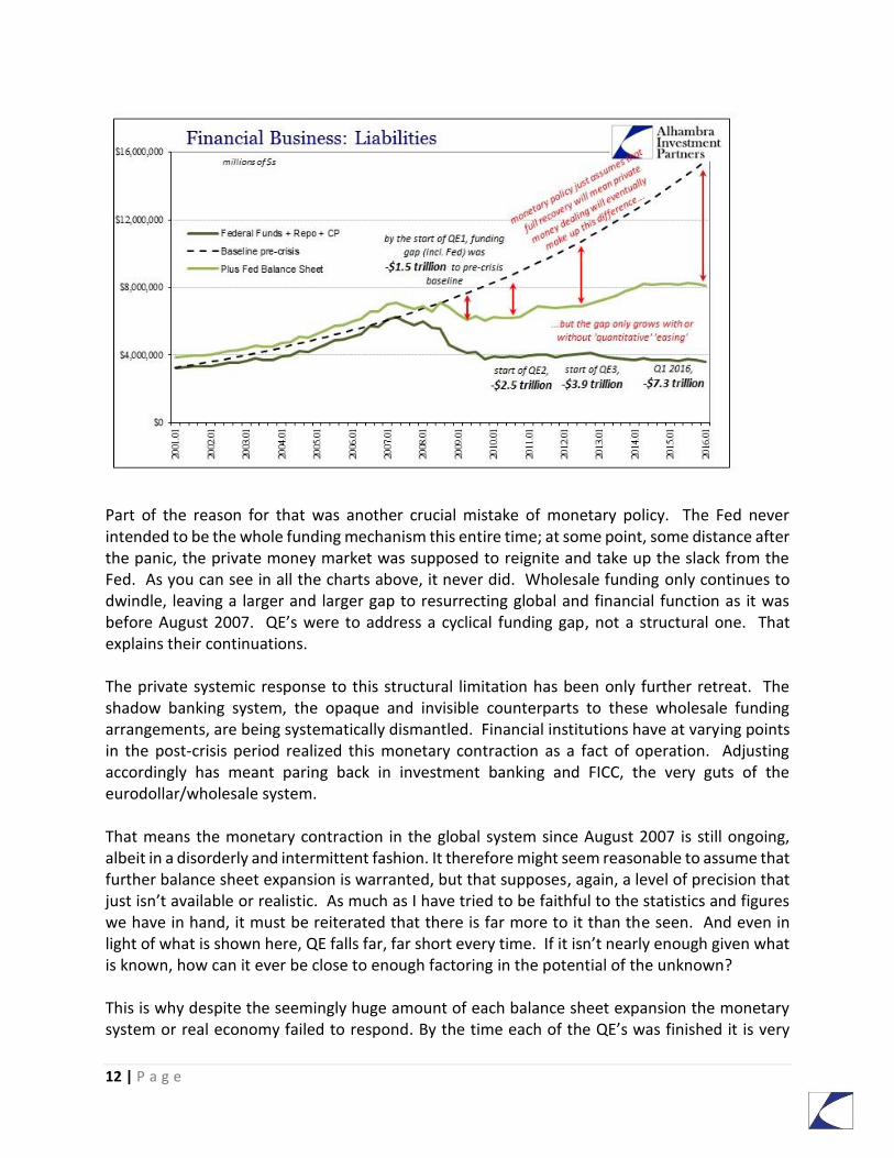
Part of the reason for that was another crucial mistake of monetary policy. The Fed never intended to be the whole funding mechanism this entire time; at some point, some distance after the panic, the private money market was supposed to reignite and take up the slack from the Fed. As you can see in all the charts above, it never did. Wholesale funding only continues to dwindle, leaving a larger and larger gap to resurrecting global and financial function as it was before August 2007. QE’s were to address a cyclical funding gap, not a structural one. That explains their continuations. The private systemic response to this structural limitation has been only further retreat. The shadow banking system, the opaque and invisible counterparts to these wholesale funding arrangements, are being systematically dismantled. Financial institutions have at varying points in the post-crisis period realized this monetary contraction as a fact of operation. Adjusting accordingly has meant paring back in investment banking and FICC, the very guts of the eurodollar/wholesale system. That means the monetary contraction in the global system since August 2007 is still ongoing, albeit in a disorderly and intermittent fashion. It therefore might seem reasonable to assume that further balance sheet expansion is warranted, but that supposes, again, a level of precision that just isn’t available or realistic. As much as I have tried to be faithful to the statistics and figures we have in hand, it must be reiterated that there is far more to it than the seen. And even in light of what is shown here, QE falls far, far short every time. If it isn’t nearly enough given what is known, how can it ever be close to enough factoring in the potential of the unknown? This is why despite the seemingly huge amount of each balance sheet expansion the monetary system or real economy failed to respond. By the time each of the QE’s was finished it is very

13 | P a g e

likely the gap had only further grown in the manner suggested on the charts above. In the context of QE, we have no realistic idea just how much of a funding gap there is – but we do have overflowing hints and suggestions that it is large and getting larger all the time. This is the true essence of the “dollar” supply problem. The nature of it is not just the quantitative shortfall in wholesale funding, but also the qualitative shortfall. While there is every reason to suspect the size of each intervention will never be enough, there are also perhaps more important reasons to cast doubt on whether bank reserves even equate to “easing” in the eurodollar context. SECTION 2: QUALITATIVE CONTRACTION The eurodollar expansion globally was as much about its forms and not purely a matter of volume. This gets to the very basic difficulty in trying to define a eurodollar in the first place. The eurodollar is not a thing like a dollar is a thing; it is, rather, a system of financial standards and protocols that allow financial business to be conducted globally among very disparate systems. Among the primary forms of eurodollar protocols are derivatives, especially swaps. From the earliest days in the 1960’s, swaps have formed the basis of operation. These are very difficult concepts to grasp and the biggest barrier to more complete monetary understanding. By not being able to penetrate the dense and often technical nature of swaps, observers are left with an incomplete understanding of the true, comprehensive nature of both the crisis and post-crisis age. Without that complete view, too much is left unknown and unanswered to be able to judge something like QE. To illustrate this point, I will use a specific example from the crisis period. On Page 33 of its 2007 Annual Report, AIG noted in Management’s Discussion and Analysis of Financial Condition and Results of Operation for its Financial Services Division that:

The ongoing disruption in the U.S. residential mortgage and credit markets and the recent downgrades of residential mortgage-backed securities and CDO securities by rating agencies continue to adversely affect the fair value of the super senior credit default swap portfolio written by AIGFP. AIG expects that continuing limitations on the availability of market observable data will affect AIG’s determinations of the fair value of these derivatives, including by preventing AIG, for the foreseeable future, from recognizing the beneficial effect of the differential between credit spreads used to price a credit default swap and spreads implied from prices of the CDO bonds referenced by such swap.

The company had written CDS for hundreds of billions in securities. As the prices of those securities began to fall and began to further point in the wrong direction, the company was trying to say - without saying it too clearly or loudly - that it might be a big problem in the future. Liquidity was the culprit, as AIG was claiming that CDS prices were not reflective of underlying

14 | P a g e

“value” implied from the reference securities. The problem in these kinds of securities, liquid or not, is just how much inference (mathematical) is required at each and every step. The company notes that its counterparties were not hedge funds seeking to hedge their holdings, but rather:

Approximately $379 billion of the $527 billion in notional exposure on AIGFP’s super senior credit default swap portfolio as of December 31, 2007 were written to facilitate regulatory capital relief for financial institutions primarily in Europe.

This is what I call “math as money.” Banks, primarily European in this instance, would pair CDS written by a highly rated counterparty, such as AIG, with specific parts of their fixed income portfolios in order to reduce their capital weighting. There was great demand for this in the super senior tranches of securitized structures because they were the largest parts and thought to be the least risky. That means companies like AIG would write protection for a relatively low premium which the bank could then use to significantly reduce its capital footprint, both sides thinking they had cooked up the proverbial free lunch or invented the financial equivalent of a perpetual motion machine. The capital ratio guidance of the Basel framework opens the door to such regulatory leverage. Basel assigned “risk” by bucket (now by less rigid categories), meaning that more risky assets as defined by the regulatory framework would require more capital offset. A mortgage loan, for instance, was required to be charged dollar for dollar (100%), meaning that for every $1 principle of the loan $1 would go into the risk-weighted asset calculation that determines capital ratios. If, however, the bank could find a compliant means to transform that mortgage loan into a lower bucket security, say 80%, then for every $1 in loans only $0.80 would be added to the total of risk weighted assets. Credit default swaps were used heavily in this manner, as AIG’s 2007 annual report spells out. We don’t know the exact effect of just how much “capital relief” was provided, or to what scale $379 billion in notional, off-balance sheet CDS might provide, we can only reasonably assume that it did and did so significantly. A stylized example of this process is as follows (with overly simplistic assumptions used in the interest of ease and clarity of understanding the general processes, not with the intent to provide a realistic re-creation):

15 | P a g e

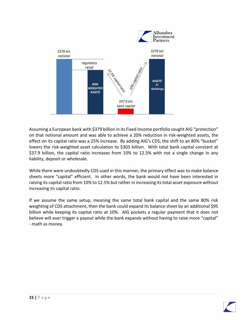
Assuming a European bank with $379 billion in its Fixed Income portfolio sought AIG “protection” on that notional amount and was able to achieve a 20% reduction in risk-weighted assets, the effect on its capital ratio was a 25% increase. By adding AIG’s CDS, the shift to an 80% “bucket” lowers the risk-weighted asset calculation to $303 billion. With total bank capital constant at $37.9 billion, the capital ratio increases from 10% to 12.5% with not a single change in any liability, deposit or wholesale. While there were undoubtedly CDS used in this manner, the primary effect was to make balance sheets more “capital” efficient. In other words, the bank would not have been interested in raising its capital ratio from 10% to 12.5% but rather in increasing its total asset exposure without increasing its capital ratio. If we assume the same setup, meaning the same total bank capital and the same 80% risk weighting of CDS attachment, then the bank could expand its balance sheet by an additional $95 billion while keeping its capital ratio at 10%. AIG pockets a regular payment that it does not believe will ever trigger a payout while the bank expands without having to raise more “capital” - math as money.

16 | P a g e

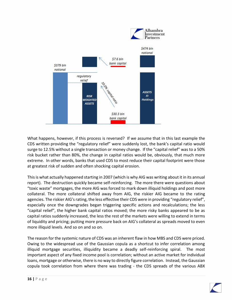
What happens, however, if this process is reversed? If we assume that in this last example the CDS written providing the “regulatory relief” were suddenly lost, the bank’s capital ratio would surge to 12.5% without a single transaction or money change. If the “capital relief” was to a 50% risk bucket rather than 80%, the change in capital ratios would be, obviously, that much more extreme. In other words, banks that used CDS to most reduce their capital footprint were those at greatest risk of sudden and often shocking capital erosion. This is what actually happened starting in 2007 (which is why AIG was writing about it in its annual report). The destruction quickly became self-reinforcing. The more there were questions about “toxic waste” mortgages, the more AIG was forced to mark down illiquid holdings and post more collateral. The more collateral shifted away from AIG, the riskier AIG became to the rating agencies. The riskier AIG’s rating, the less effective their CDS were in providing “regulatory relief”, especially once the downgrades began triggering specific actions and recalculations; the less “capital relief”, the higher bank capital ratios moved; the more risky banks appeared to be as capital ratios suddenly increased, the less the rest of the markets were willing to extend in terms of liquidity and pricing; putting more pressure back on AIG’s collateral as spreads moved to even more illiquid levels. And so on and so on. The reason for the systemic nature of CDS was an inherent flaw in how MBS and CDS were priced. Owing to the widespread use of the Gaussian copula as a shortcut to infer correlation among illiquid mortgage securities, illiquidity became a deadly self-reinforcing spiral. The most important aspect of any fixed income pool is correlation; without an active market for individual loans, mortgage or otherwise, there is no way to directly figure correlation. Instead, the Gaussian copula took correlation from where there was trading - the CDS spreads of the various ABX

17 | P a g e

indices and wherever else volume was sufficient. In basic terms, the Gaussian copula assumed a higher degree of correlation where curves were similar. In the growing fear and illiquidity of 2007, the resulting heightened demand for hedging had the effect of pushing CDS spreads and curves all in the same direction at the same time. To correlation trading and pricing, the Gaussian copula viewed that as rising correlation, thus reducing prices of securitization tranches without any actual trading in them (the huge downside of black box pricing models). This repricing through illiquidity and inference was heaviest at the ends, either the equity piece or the super senior where correlation exhibits a “smile” or skew – if correlation rises to 100%, that is either really good or really bad because it means either no one will default or everyone will. In super senior tranches where AIG was most active in writing protection, rising correlation very quickly introduces significant modeled risk even for a super senior that was believed at the start as close to “risk free” as a UST bond. AIG was brought down by collateral, not losses. In fact, the Federal Reserve made money on its Maiden Lane holdings, the so-called bailout of AIG’s CDS and other portfolios. But you can understand why they did so, even if you don’t agree with the action. The company had written $379 billion in notional CDS that was applied primarily to European bank “capital relief.” We don’t have any idea how much relief that provided nor the scale of its association. In the simple examples I used above, math as money, I applied $379 billion in notional against one bank’s hypothetical $379 billion fixed income portfolio. In reality, it is very likely that those AIG CDS were supporting “capital relief” on multiples of that amount. If AIG had failed in September 2008, aggregate European bank capital would have suffered another huge blow at a time when it was already seriously questionable - and in Europe where this onshore/offshore divide was already the primary factor in systemic panic. In fact, that was a primary reason for the uncertainty to that point, where questionable math-as-money was being unwound in disorderly fashion to begin with. This is the eurodollar system as it truly is in its multi-dimensional forms, where various financial firms provide different kinds of balance sheet “capacity” so that other financial firms can expand their balance sheets into more wholesale money and credit. Take away the trading of risk absorption capacity, not just CDS, and the whole systemic chain tumbles like dominos. From this perspective, it is much easier to appreciate why the Fed failed so thoroughly during the crisis period. The appeal first of interest rate targeting and the implicit support of private money bank reserves just do not enter into this wholesale process in any way. The problem was not money dealing in the traditional sense of tangible monetary units. It was overall risk capacity that could do nothing but shrink because the prior assumptions (math) were being revealed as invalid. The only possible “monetary policy” that might have had a chance of success was for the Fed to not just take over AIG and others’ CDS portfolios, but to also continue writing CDS on their behalf – the dollar shortage at that time throughout 2008 was as much CDS capacity as dollars. The “funding” shortfall in this core aspect was far beyond any capacity provided by bank reserves or anything currently available to the Federal Reserve.

18 | P a g e

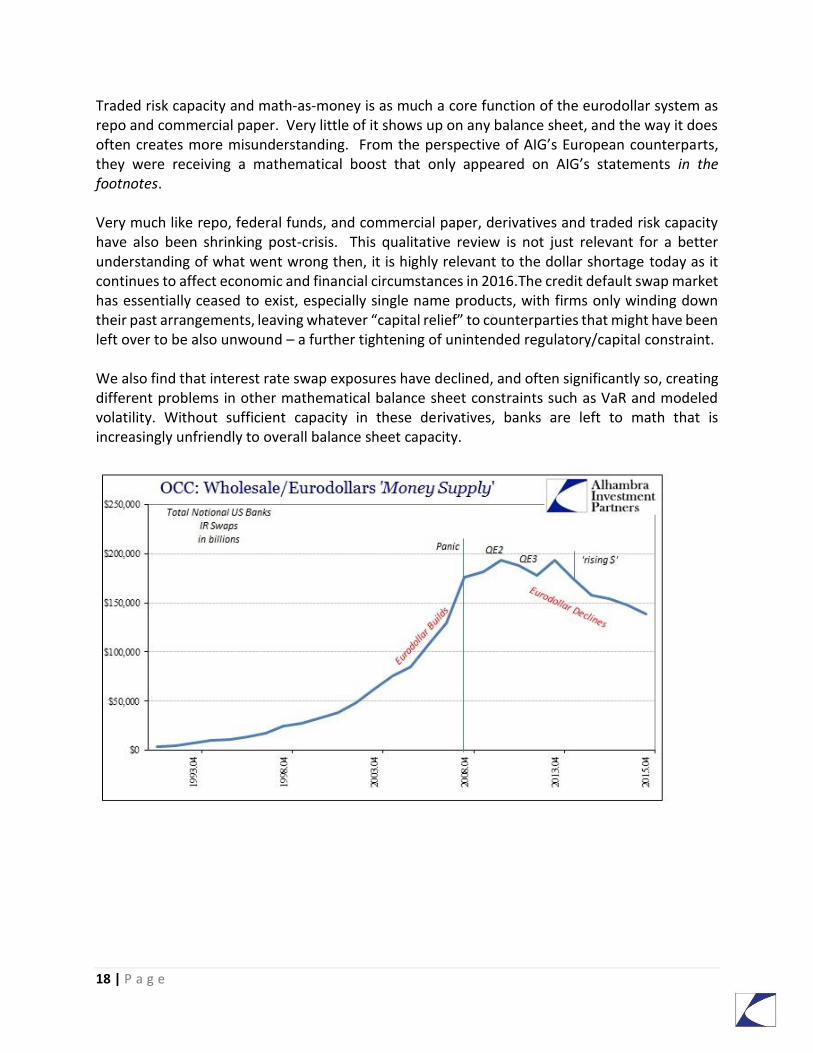
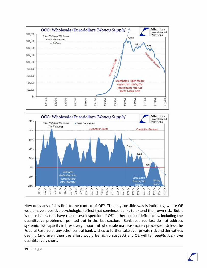
Traded risk capacity and math-as-money is as much a core function of the eurodollar system as repo and commercial paper. Very little of it shows up on any balance sheet, and the way it does often creates more misunderstanding. From the perspective of AIG’s European counterparts, they were receiving a mathematical boost that only appeared on AIG’s statements in the footnotes. Very much like repo, federal funds, and commercial paper, derivatives and traded risk capacity have also been shrinking post-crisis. This qualitative review is not just relevant for a better understanding of what went wrong then, it is highly relevant to the dollar shortage today as it continues to affect economic and financial circumstances in 2016.The credit default swap market has essentially ceased to exist, especially single name products, with firms only winding down their past arrangements, leaving whatever “capital relief” to counterparties that might have been left over to be also unwound – a further tightening of unintended regulatory/capital constraint. We also find that interest rate swap exposures have declined, and often significantly so, creating different problems in other mathematical balance sheet constraints such as VaR and modeled volatility. Without sufficient capacity in these derivatives, banks are left to math that is increasingly unfriendly to overall balance sheet capacity.

19 | P a g e

How does any of this fit into the context of QE? The only possible way is indirectly, where QE would have a positive psychological effect that convinces banks to extend their own risk. But it is these banks that have the closest inspection of QE’s other serious deficiencies, including the quantitative problems I pointed out in the last section. Bank reserves just do not address systemic risk capacity in these very important wholesale math-as-money processes. Unless the Federal Reserve or any other central bank wishes to further take over private risk and derivatives dealing (and even then the effort would be highly suspect) any QE will fall qualitatively and quantitatively short.

20 | P a g e

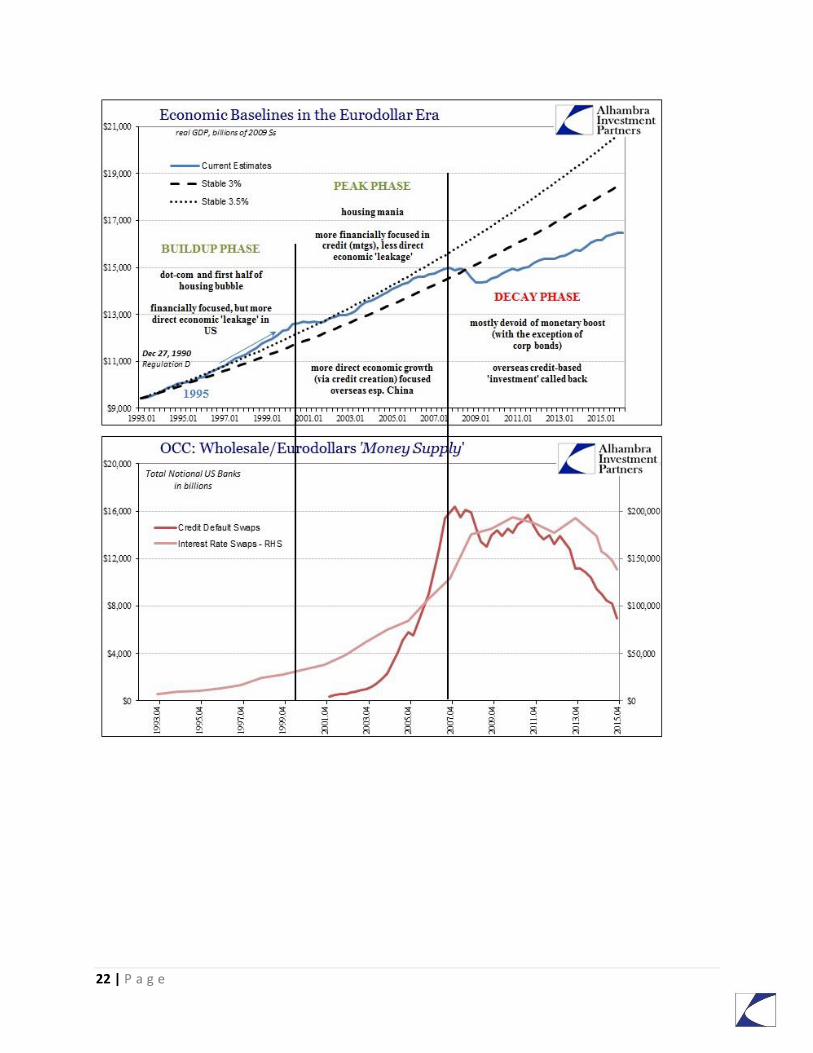
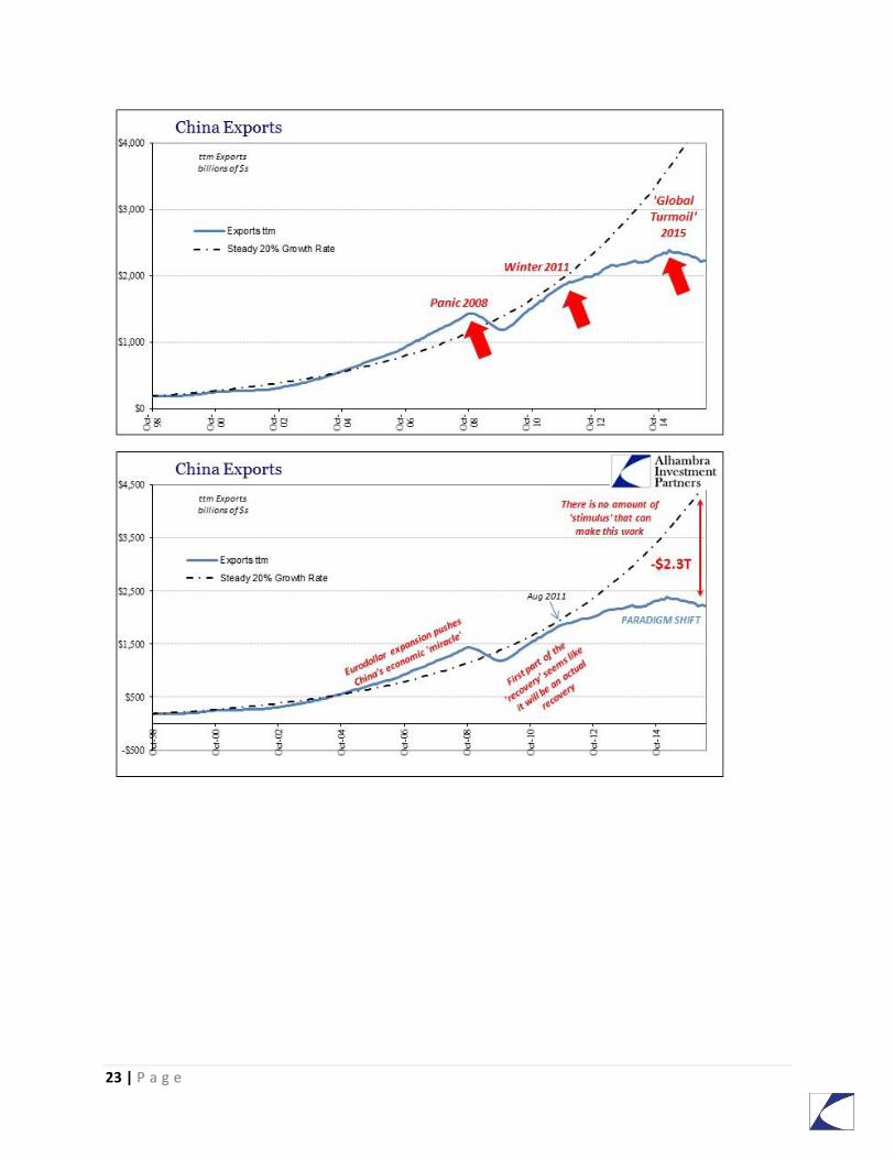
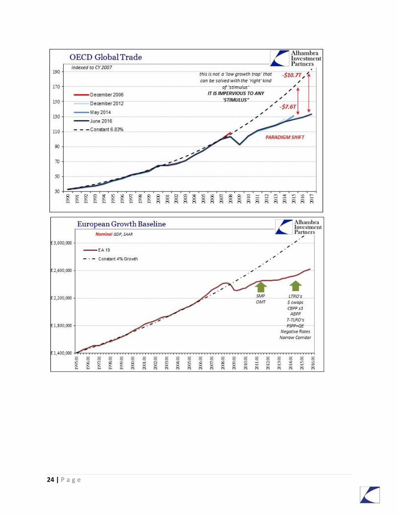
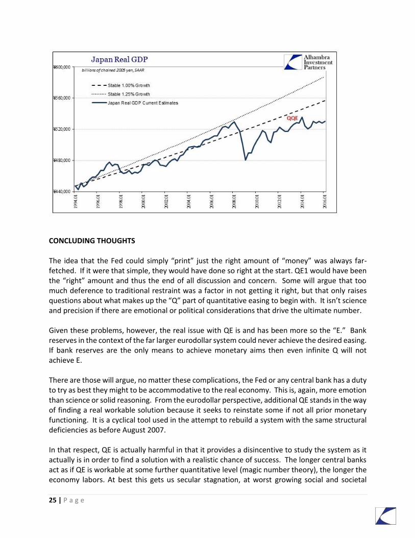
SECTION 3: ECONOMIC IMPLICATIONS OF WHOLESALE CONTRACTION The textbook economic response to monetary contraction is deflation - or at least disinflation - severe declines in commodity prices and increasingly depressive economic conditions. That describes very well the global economy, especially since 2012. In case after case, we find the same pattern of monetary behavior being mimicked in the real economy. That has led to enormous confusion in orthodox economics because it sees the Fed’s balance sheet expansion in a vacuum – as monetary expansion. Instead, as only partially demonstrated here, the Fed’s balance sheet was only a small offset factor to an otherwise enormous, wide-ranging, and ongoing contraction. This monetary contraction is multi-dimensional and it is highly unlikely that financial conditions will ever realign such that the global economy can be led back to its pre-crisis condition. There is no specific, quantitative amount of balance sheet expansion that leads to a specific increase in bank reserves that fixes this imbalance. The eurodollar system’s retreat or decay is far greater than anything any central bank can counterpoise. Even if the Fed were to obtain both the will and statutory authority to take over more of these contracting eurodollar functions, it would still not be enough because of how much is still unknown. This sustained contraction in eurodollar “money” is incorporated in almost exactly the same fashion in the global economy in almost textbook fashion, including specific eurodollar references to amplifications of the decay process (notably 2012 after the 2011 redo funding crisis and the 2014 “rising dollar” of further eurodollar retreat):

21 | P a g e

22 | P a g e

23 | P a g e

24 | P a g e

25 | P a g e

CONCLUDING THOUGHTS The idea that the Fed could simply “print” just the right amount of “money” was always far-fetched. If it were that simple, they would have done so right at the start. QE1 would have been the “right” amount and thus the end of all discussion and concern. Some will argue that too much deference to traditional restraint was a factor in not getting it right, but that only raises questions about what makes up the “Q” part of quantitative easing to begin with. It isn’t science and precision if there are emotional or political considerations that drive the ultimate number. Given these problems, however, the real issue with QE is and has been more so the “E.” Bank reserves in the context of the far larger eurodollar system could never achieve the desired easing. If bank reserves are the only means to achieve monetary aims then even infinite Q will not achieve E. There are those will argue, no matter these complications, the Fed or any central bank has a duty to try as best they might to be accommodative to the real economy. This is, again, more emotion than science or solid reasoning. From the eurodollar perspective, additional QE stands in the way of finding a real workable solution because it seeks to reinstate some if not all prior monetary functioning. It is a cyclical tool used in the attempt to rebuild a system with the same structural deficiencies as before August 2007. In that respect, QE is actually harmful in that it provides a disincentive to study the system as it actually is in order to find a solution with a realistic chance of success. The longer central banks act as if QE is workable at some further quantitative level (magic number theory), the longer the economy labors. At best this gets us secular stagnation, at worst growing social and societal

26 | P a g e

disruption. Current monetary policy is an attempt to maintain an unworkable status quo; the eurodollar contraction is an oncoming paradigm shift. The period since 2008 with its numerous monetary mistakes, was a wasted opportunity to address the systemic instability of the Eurodollar standard. If there is a dollar shortage - and the evidence is overwhelming there is - then it will not be solved through more QE no matter how large. The problem is not that there might be a change in demand for dollars, it is rather that there is no capacity to meet it. Should the Fed engage in another round of balance sheet expansion it is very likely to be overwhelmed by the continued decay in the same, much larger and more comprehensive eurodollar manner. They could start another $2 trillion today and in a year we would likely be wondering where it all went, why there is yet again no sign of its intended effects. The global economy and the eurodollar financial system both in general outline and in specific instances follow the condition of systemic monetary contraction in all its forms. The Federal Reserve in 2006 when it ended M3, the leading edge of wholesale eurodollars, declared that it “does not appear to convey any additional information about economic activity that is not already embodied in M2 and has not played a role in the monetary policy process for many years.” What we find instead is that everything about economic activity is in those parts of M3 and whatever else lies beyond them. The only relevance to true monetary policy is in those pieces. QE is essentially inaction; the global economy awaits a real solution, one that actually addresses the dollar shortage.

Jeffrey P. Snider

Chief Investment Strategist of Alhambra Investment Partners, LLC

“Wealth preservation and accumulation through thoughtful investing.”

For information on Alhambra Investment Partners’ money management services and

global portfolio approach to capital preservation, Joe Calhoun can be reached at:

786-249-3773

JSnider@alhambrapartners.com