Embed Size (px)
Citation preview
Why Piketty Says r − g Matters for Inequality
Supplementary Lecture Notes “Income and Wealth Distribution”
Benjamin Moll
Princeton
June 1, 2014
1 / 25
These Notes
My version of a hybrid of
1 Section 5.4 of Piketty and Zucman (2014)http://gabriel-zucman.eu/files/PikettyZucman2014HID.pdf
2 Benhabib, Bisin and Zhu (2013)http://www.econ.nyu.edu/user/benhabib/lineartail31.pdf
Warning: high probability of algebra mistakes. If you find one, please email me
2 / 25
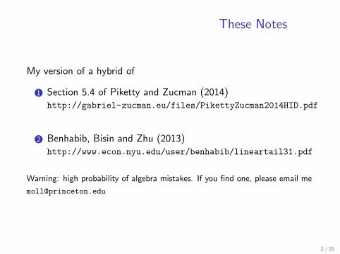
These NotesSummary:
• Standard explanation of high observed wealth concentration(e.g. top 1% own 30%): idiosyncratic capital income risk
• In theories with capital income risk, r − g is one maindeterminant of top wealth inequality
• Theory suggests slight modification: r − g − c where c is themarginal propensity to consume out of wealth for rich people
What these notes are not about:
• the aggregate capital-output ratio K/Y : different story(inequality across groups)
• see Piketty and Zucman (2014)
• and critical reviews by Ray and Krusell-Smith:http://www.econ.nyu.edu/user/debraj/Papers/Piketty.pdf
http://aida.wss.yale.edu/smith/piketty1.pdf
3 / 25
Outline
1 Simplest possible case
• Brownian capital income risk
• exogenous MPC
2 Generalizations
• endogenous savings/MPC
• labor income risk
• more general capital income processes
3 Transition dynamics
4 / 25
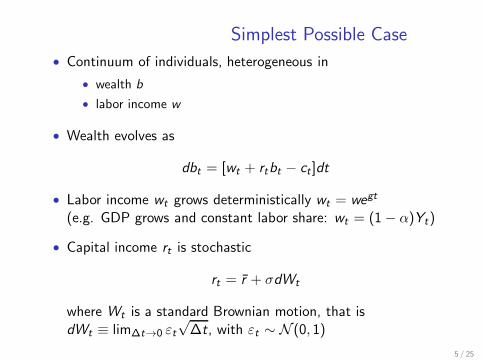
Simplest Possible Case
• Continuum of individuals, heterogeneous in
• wealth b
• labor income w
• Wealth evolves as
dbt = [wt + rtbt − ct ]dt
• Labor income wt grows deterministically wt = wegt
(e.g. GDP grows and constant labor share: wt = (1− α)Yt)
• Capital income rt is stochastic
rt = r + σdWt
where Wt is a standard Brownian motion, that isdWt ≡ lim∆t→0 εt
√∆t, with εt ∼ N (0, 1)
5 / 25
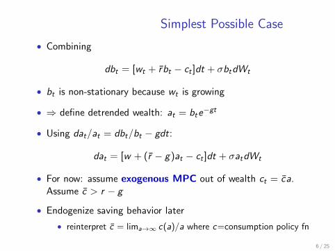
Simplest Possible Case
• Combining
dbt = [wt + r bt − ct ]dt + σbtdWt
• bt is non-stationary because wt is growing
• ⇒ define detrended wealth: at = bte−gt
• Using dat/at = dbt/bt − gdt:
dat = [w + (r − g)at − ct ]dt + σatdWt
• For now: assume exogenous MPC out of wealth ct = ca.Assume c > r − g
• Endogenize saving behavior later
• reinterpret c = lima→∞ c(a)/a where c=consumption policy fn
6 / 25
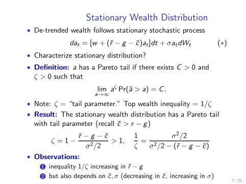
Stationary Wealth Distribution• De-trended wealth follows stationary stochastic process
dat = [w + (r − g − c)at ]dt + σatdWt (∗)• Characterize stationary distribution?
• Definition: a has a Pareto tail if there exists C > 0 andζ > 0 such that
lima→∞
aζ Pr(a > a) = C .
• Note: ζ = “tail parameter.” Top wealth inequality = 1/ζ
• Result: The stationary wealth distribution has a Pareto tailwith tail parameter (recall c > r − g)
ζ = 1− r − g − c
σ2/2> 1,
1
ζ=
σ2/2
σ2/2− (r − g − c)
• Observations:
1 inequality 1/ζ increasing in r − g
2 but also depends on c , σ (decreasing in c , increasing in σ)7 / 25
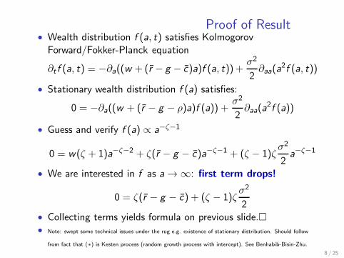
Proof of Result• Wealth distribution f (a, t) satisfies KolmogorovForward/Fokker-Planck equation
∂t f (a, t) = −∂a((w + (r − g − c)a)f (a, t)) +σ2
2∂aa(a
2f (a, t))
• Stationary wealth distribution f (a) satisfies:
0 = −∂a((w + (r − g − ρ)a)f (a)) +σ2
2∂aa(a
2f (a))
• Guess and verify f (a) ∝ a−ζ−1
0 = w(ζ + 1)a−ζ−2 + ζ(r − g − c)a−ζ−1 + (ζ − 1)ζσ2
2a−ζ−1
• We are interested in f as a → ∞: first term drops!
0 = ζ(r − g − c) + (ζ − 1)ζσ2
2• Collecting terms yields formula on previous slide.�• Note: swept some technical issues under the rug e.g. existence of stationary distribution. Should follow
from fact that (∗) is Kesten process (random growth process with intercept). See Benhabib-Bisin-Zhu.
8 / 25
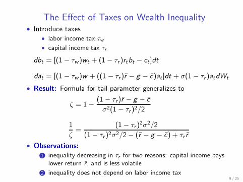
The Effect of Taxes on Wealth Inequality• Introduce taxes
• labor income tax τw• capital income tax τr
dbt = [(1− τw )wt + (1− τr )rtbt − ct ]dt
dat = [(1− τw )w + ((1 − τr )r − g − c)at ]dt + σ(1− τr )atdWt
• Result: Formula for tail parameter generalizes to
ζ = 1− (1− τr )r − g − c
σ2(1− τr )2/2
1
ζ=
(1− τr )2σ2/2
(1− τr )2σ2/2− (r − g − c) + τr r
• Observations:
1 inequality decreasing in τr for two reasons: capital income payslower return r , and is less volatile
2 inequality does not depend on labor income tax9 / 25
Discussion• Other sources of randomness in wealth growth
• Piketty-Zucman (Section 5.4) have stochasticsavings/bequests rather than stochastic capital income
• this is mathematically isomorphic: everything identical if set
rt = r , ct(a) = ca+ σadWt
• what matters is that at follows random growth process like (∗)• randomness in bequests would work similarly (e.g. in more
general model with OLG structure and Poisson death)
• while mathematically isomorphic, economics obviously different
• Partial vs. General Equilibrium
• obviously both r and g are endogenous, and so the aboveanalysis is potentially misleading
• GE extension interesting/desirable, especially forcounterfactuals/policy
• but PE with exogenous r , g=useful starting point
10 / 25
Generalizations
1 Optimally chosen savings
2 stochastic labor income wt
3 more general process for capital income rt
11 / 25
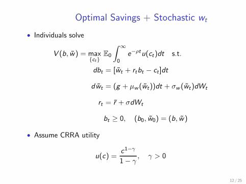
Optimal Savings + Stochastic wt
• Individuals solve
V (b, w) = max{ct}
E0
∫ ∞
0e−ρtu(ct)dt s.t.
dbt = [wt + rtbt − ct ]dt
dwt = (g + µw (wt))dt + σw (wt)dWt
rt = r + σdWt
bt ≥ 0, (b0, w0) = (b, w )
• Assume CRRA utility
u(c) =c1−γ
1− γ, γ > 0
12 / 25
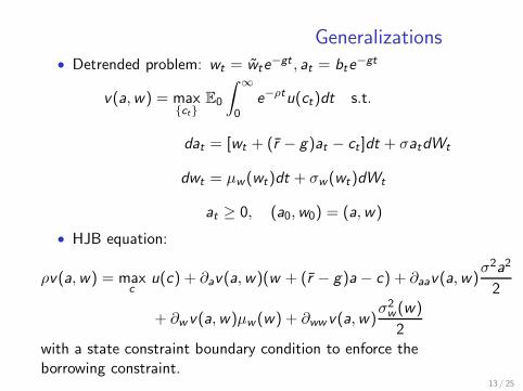
Generalizations• Detrended problem: wt = wte
−gt , at = bte−gt
v(a,w) = max{ct}
E0
∫ ∞
0e−ρtu(ct)dt s.t.
dat = [wt + (r − g)at − ct ]dt + σatdWt
dwt = µw (wt)dt + σw (wt)dWt
at ≥ 0, (a0,w0) = (a,w)
• HJB equation:
ρv(a,w) = maxc
u(c) + ∂av(a,w)(w + (r − g)a − c) + ∂aav(a,w)σ2a2
2
+ ∂wv(a,w)µw (w) + ∂wwv(a,w)σ2w (w)
2with a state constraint boundary condition to enforce theborrowing constraint.
13 / 25
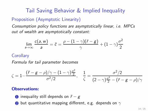
Tail Saving Behavior & Implied Inequality
Proposition (Asymptotic Linearity)
Consumption policy functions are asymptotically linear, i.e. MPCs
out of wealth are asymptotically constant:
lima→∞
c(a,w)
a= c =
ρ− (1− γ)(r − g)
γ+ (1− γ)
σ2
2
Corollary
Formula for tail parameter becomes
ζ = 1−(r − g − ρ)/γ − (1− γ)σ2
2
σ2/2,
1
ζ=
σ2/2
(2− γ)σ2
2 − (r − g − ρ)/γ
Observations:
1 inequality still depends on r − g
2 but quantitative mapping different, e.g. depends on γ14 / 25
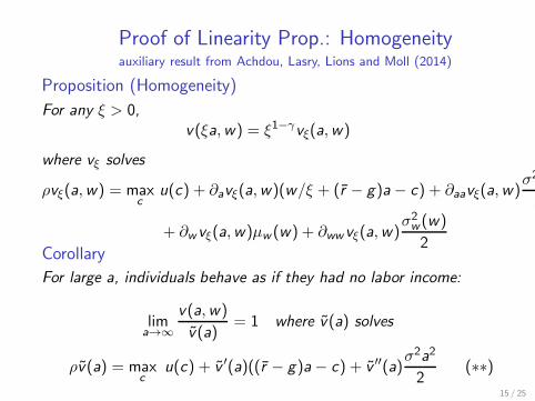
Proof of Linearity Prop.: Homogeneityauxiliary result from Achdou, Lasry, Lions and Moll (2014)
Proposition (Homogeneity)
For any ξ > 0,v(ξa,w) = ξ1−γvξ(a,w)
where vξ solves
ρvξ(a,w) = maxc
u(c) + ∂avξ(a,w)(w/ξ + (r − g)a − c) + ∂aavξ(a,w)σ2
2
+ ∂wvξ(a,w)µw (w) + ∂wwvξ(a,w)σ2w (w)
2Corollary
For large a, individuals behave as if they had no labor income:
lima→∞
v(a,w)
v(a)= 1 where v(a) solves
ρv(a) = maxc
u(c) + v ′(a)((r − g)a − c) + v ′′(a)σ2a2
2(∗∗)
15 / 25
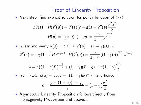
Proof of Linearity Proposition• Next step: find explicit solution for policy function of (∗∗)
ρv(a) =H(v ′(a)) + v ′(a)(r − g)a + v ′′(a)σ2a2
2
H(p) = maxc
u(c)− pc =γ
1− γp
γ−1γ
• Guess and verify v(a) = Ba1−γ , v ′(a) = (1− γ)Ba−γ ,
v ′′(a) = −γ(1−γ)Ba−γ−1, H(v ′(a)) =γ
1− γ((1−γ)B)
γ−1γ a1−γ
ρ = γ((1 − γ)B)−1γ + (1− γ)(r − g)− γ(1− γ)
σ2
2
• from FOC, c(a) = ca, c = ((1 − γ)B)−1/γ and hence
c =ρ− (1− γ)(r − g)
γ+ (1− γ)
σ2
2
• Asymptotic Linearity Proposition follows directly fromHomogeneity Proposition and above.�
16 / 25
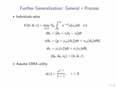
Further Generalization: General r Process
• Individuals solve
V (b, w , r) = max{ct}
E0
∫ ∞
0e−ρtu(ct)dt s.t.
dbt = [wt + rtbt − ct ]dt
dwt = (g + µw (wt))dt + σw (wt)dWt
drt = µr (rt))dt + σr (rt)dBt
(b0, w0, r0) = (b, w , r)
• Assume CRRA utility
u(c) =c1−γ
1− γ, γ > 0
17 / 25
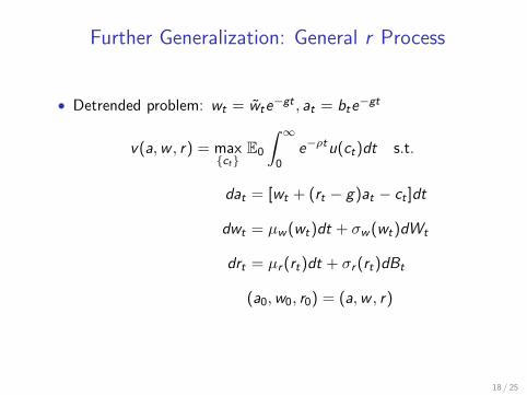
Further Generalization: General r Process
• Detrended problem: wt = wte−gt , at = bte
−gt
v(a,w , r) = max{ct}
E0
∫ ∞
0e−ρtu(ct)dt s.t.
dat = [wt + (rt − g)at − ct ]dt
dwt = µw (wt)dt + σw (wt)dWt
drt = µr (rt)dt + σr (rt)dBt
(a0,w0, r0) = (a,w , r)
18 / 25
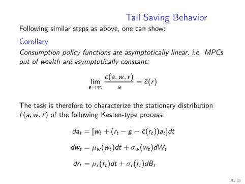
Tail Saving BehaviorFollowing similar steps as above, one can show:
Corollary
Consumption policy functions are asymptotically linear, i.e. MPCs
out of wealth are asymptotically constant:
lima→∞
c(a,w , r)
a= c(r)
The task is therefore to characterize the stationary distributionf (a,w , r) of the following Kesten-type process:
dat = [wt + (rt − g − c(rt))at ]dt
dwt = µw (wt)dt + σw (wt)dWt
drt = µr (rt)dt + σr (rt)dBt
19 / 25
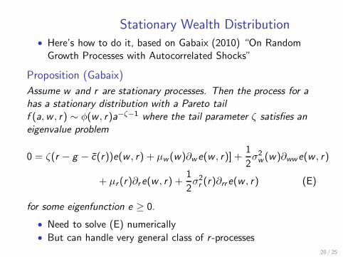
Stationary Wealth Distribution• Here’s how to do it, based on Gabaix (2010) “On RandomGrowth Processes with Autocorrelated Shocks”
Proposition (Gabaix)
Assume w and r are stationary processes. Then the process for a
has a stationary distribution with a Pareto tail
f (a,w , r) ∼ φ(w , r)a−ζ−1 where the tail parameter ζ satisfies an
eigenvalue problem
0 = ζ(r − g − c(r))e(w , r) + µw (w)∂w e(w , r)] +1
2σ2w (w)∂wwe(w , r)
+ µr (r)∂re(w , r) +1
2σ2r (r)∂rre(w , r) (E)
for some eigenfunction e ≥ 0.
• Need to solve (E) numerically• But can handle very general class of r -processes
20 / 25
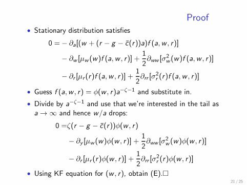
Proof• Stationary distribution satisfies
0 =− ∂a[(w + (r − g − c(r))a)f (a,w , r)]
− ∂w [µw (w)f (a,w , r)] +1
2∂ww [σ
2w (w)f (a,w , r)]
− ∂r [µr (r)f (a,w , r)] +1
2∂rr [σ
2r (r)f (a,w , r)]
• Guess f (a,w , r) = φ(w , r)a−ζ−1 and substitute in.
• Divide by a−ζ−1 and use that we’re interested in the tail asa → ∞ and hence w/a drops:
0 =ζ(r − g − c(r))φ(w , r)
− ∂y [µw (w)φ(w , r)] +1
2∂ww [σ
2w (w)φ(w , r)]
− ∂r [µr (r)φ(w , r)] +1
2∂rr [σ
2r (r)φ(w , r)]
• Using KF equation for (w , r), obtain (E).�21 / 25
Transition Dynamics
0%
10%
20%
30%
40%
50%
60%
70%
80%
90%
100%
1810 1830 1850 1870 1890 1910 1930 1950 1970 1990 2010
Sh
are
of to
p d
ecile
or
pe
rce
ntile
in
to
tal w
ea
lth
!"#$%&'(%)*+%,-&'%.("&/012%3(4$&'%*"(5/4$*&1%346%'*7'(0%*"%8/09:(%&'4"%*"%&'(%!"*&(+%;&4&(6<%
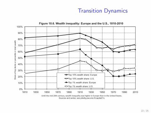
Sources and series: see piketty.pse.ens.fr/capital21c.
Figure 10.6. Wealth inequality: Europe and the U.S., 1810-2010
Top 10% wealth share: Europe
Top 10% wealth share: U.S.
Top 1% wealth share: Europe
Top 1% wealth share: U.S.
22 / 25
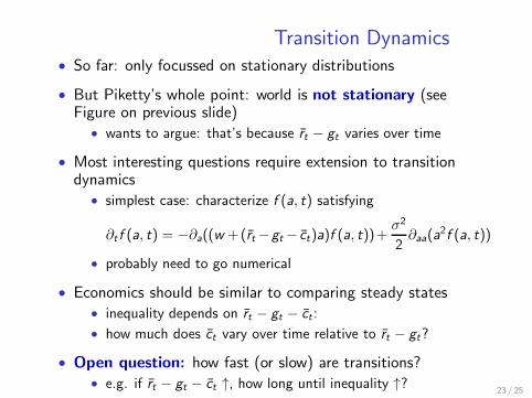
Transition Dynamics• So far: only focussed on stationary distributions
• But Piketty’s whole point: world is not stationary (seeFigure on previous slide)
• wants to argue: that’s because rt − gt varies over time
• Most interesting questions require extension to transitiondynamics
• simplest case: characterize f (a, t) satisfying
∂t f (a, t) = −∂a((w +(rt −gt − ct)a)f (a, t))+σ2
2∂aa(a
2f (a, t))
• probably need to go numerical
• Economics should be similar to comparing steady states• inequality depends on rt − gt − ct :
• how much does ct vary over time relative to rt − gt?
• Open question: how fast (or slow) are transitions?• e.g. if rt − gt − ct ↑, how long until inequality ↑?
23 / 25
Richer Models
• Why would capital income be stochastic?
• One answer: entrepreneurship
• Quadrini (1999, 2000)
• Cagetti and DeNardi (2006)
24 / 25
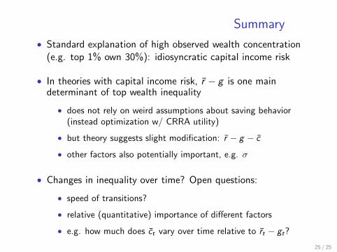
Summary
• Standard explanation of high observed wealth concentration(e.g. top 1% own 30%): idiosyncratic capital income risk
• In theories with capital income risk, r − g is one maindeterminant of top wealth inequality
• does not rely on weird assumptions about saving behavior(instead optimization w/ CRRA utility)
• but theory suggests slight modification: r − g − c
• other factors also potentially important, e.g. σ
• Changes in inequality over time? Open questions:
• speed of transitions?
• relative (quantitative) importance of different factors
• e.g. how much does ct vary over time relative to rt − gt?
25 / 25


![European Journal of Sociology ......6.6 trillion euro value of German real estate in 2008 [Voigtl€ander et al. 2008: i-iv] and 39 percent of private net wealth [Piketty and Zucman](https://img.pdfslide.us/doc/110x75/5f86703189d2e974827225e6/european-journal-of-sociology-66-trillion-euro-value-of-german-real-estate.jpg)