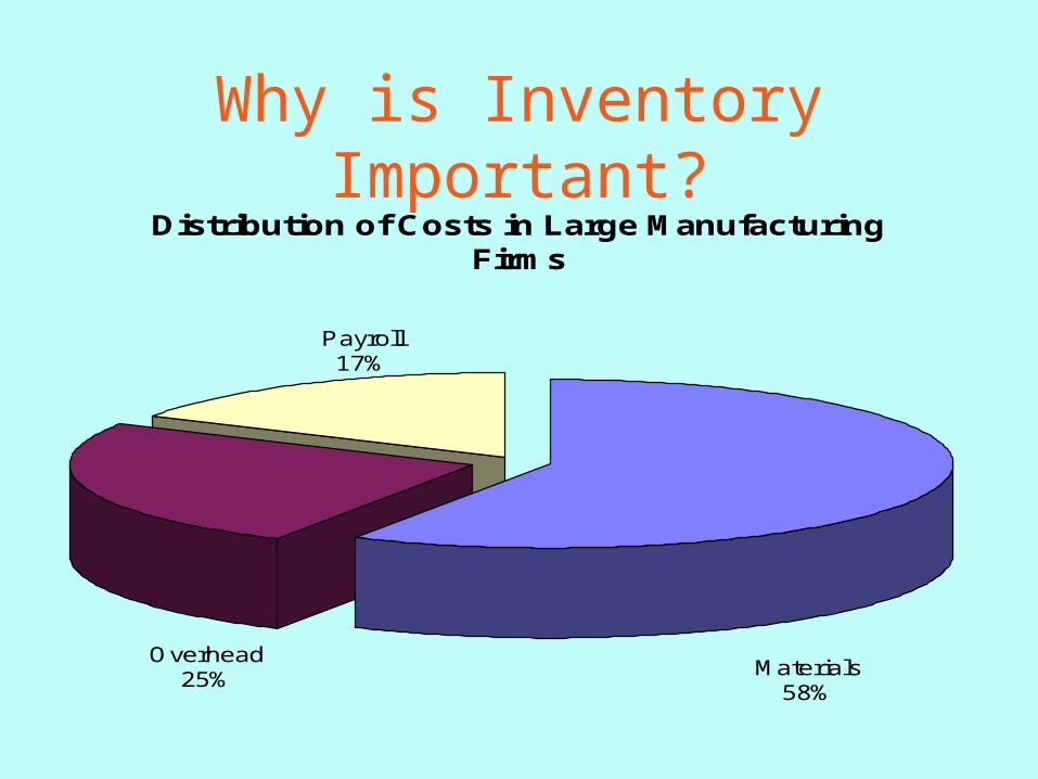
Why is Inventory Important?Distribution of Costs in Large Manufacturing

Firms

Payroll17%

Overhead25%

Materials58%

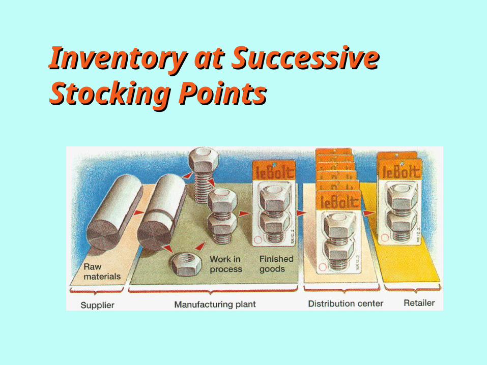
Inventory at Successive Inventory at Successive Stocking PointsStocking Points

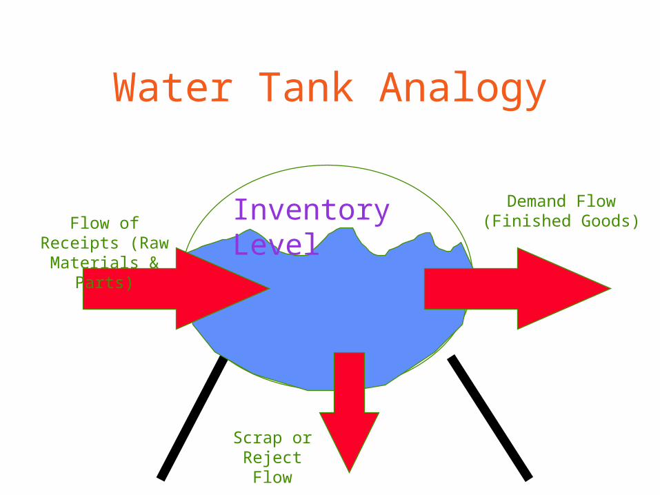
Water Tank Analogy

Flow of Receipts (Raw Materials &

Parts)

Demand Flow (Finished Goods)

Scrap or Reject Flow

Inventory Level

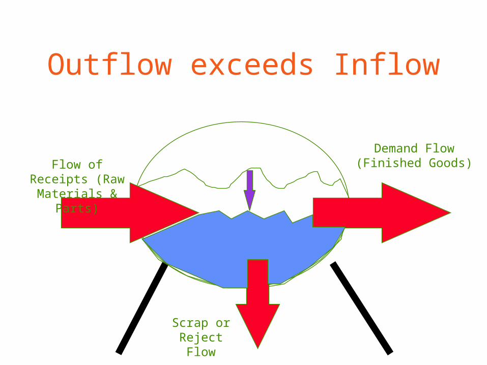
Outflow exceeds Inflow

Flow of Receipts (Raw Materials &

Parts)

Demand Flow (Finished Goods)

Scrap or Reject Flow

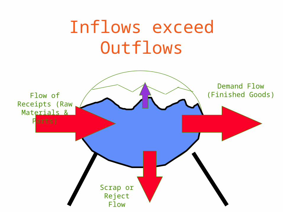
Inflows exceed Outflows

Flow of Receipts (Raw Materials &

Parts)

Demand Flow (Finished Goods)

Scrap or Reject Flow

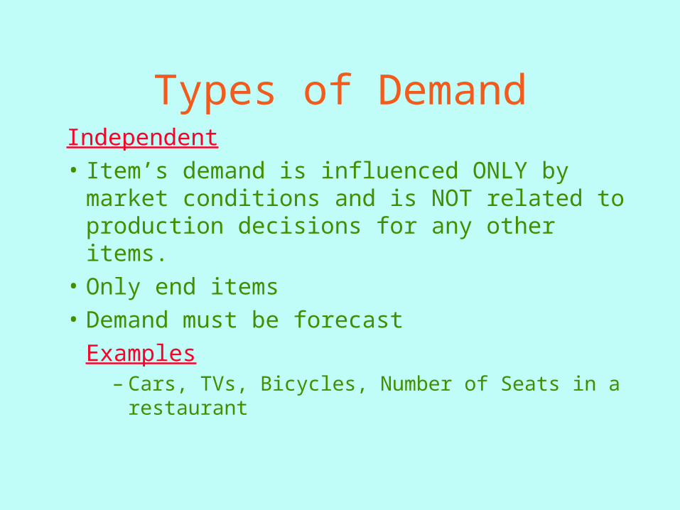
Types of DemandIndependent

• Item’s demand is influenced ONLY by market conditions and is NOT related to production decisions for any other items.

• Only end items

• Demand must be forecast

Examples– Cars, TVs, Bicycles, Number of Seats in a restaurant

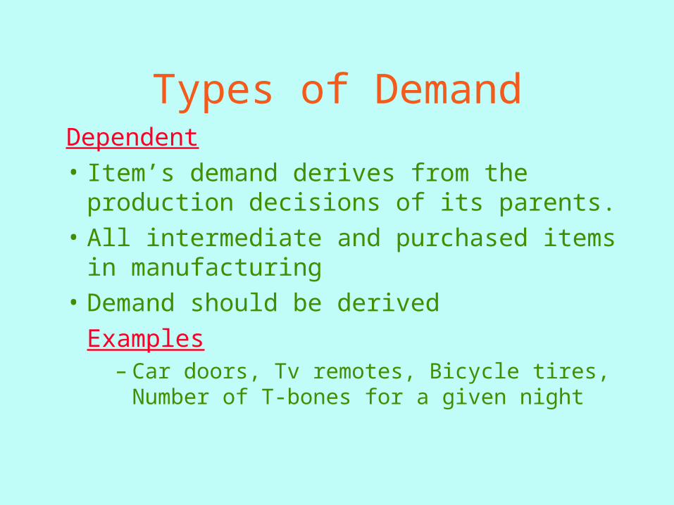
Types of DemandDependent

• Item’s demand derives from the production decisions of its parents.

• All intermediate and purchased items in manufacturing

• Demand should be derived

Examples– Car doors, Tv remotes, Bicycle tires, Number of T-

bones for a given night

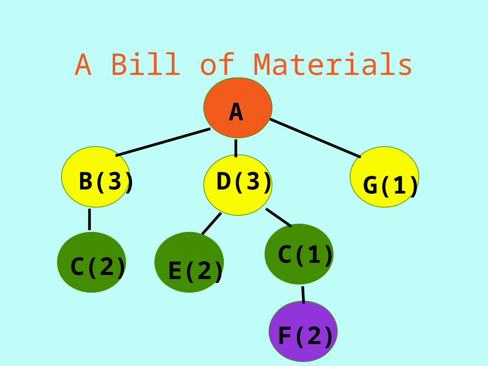
A Bill of Materials

A

B(3)

C(2) C(1)

D(3)

E(2)

F(2)

G(1)

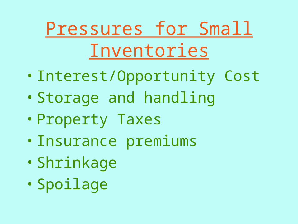
Pressures for Small Inventories

• Interest/Opportunity Cost

• Storage and handling

• Property Taxes

• Insurance premiums

• Shrinkage

• Spoilage

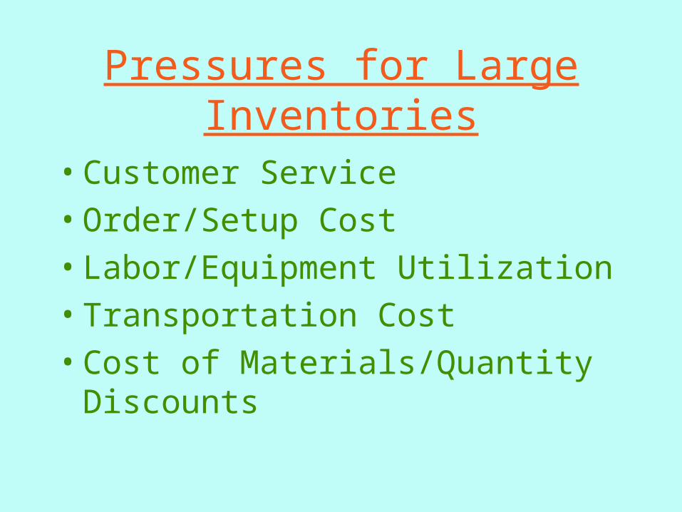
Pressures for Large Inventories

• Customer Service

• Order/Setup Cost

• Labor/Equipment Utilization

• Transportation Cost

• Cost of Materials/Quantity Discounts

The Gaming Co.

How How Much?Much? When!When!

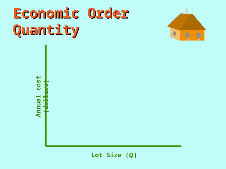
Economic Order QuantityEconomic Order QuantityA

nn

ual

co

st

(do

llars

)

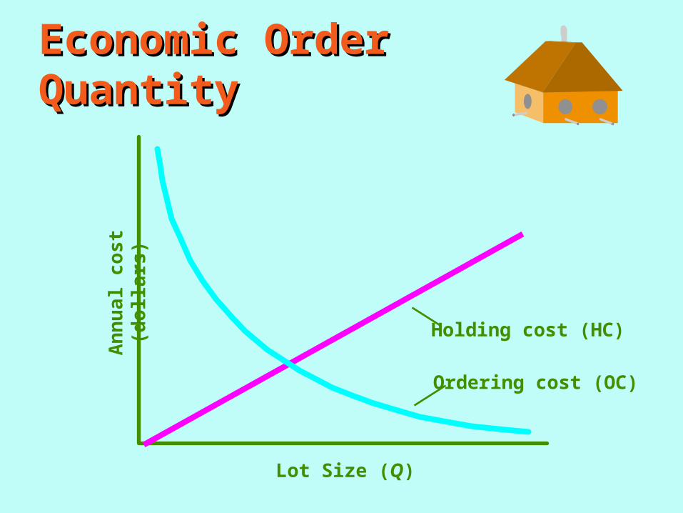
Lot Size (Q)

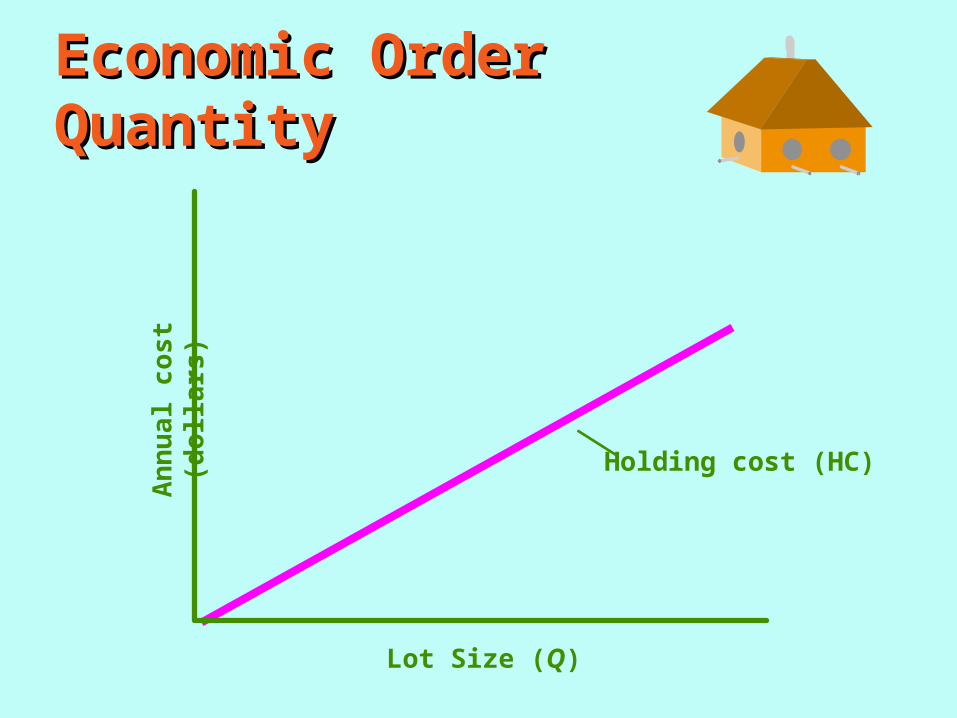
Economic Order QuantityEconomic Order QuantityA

nn

ual

co

st

(do

llars

)

Lot Size (Q)

Holding cost (HC)

Economic Order QuantityEconomic Order QuantityA

nn

ual

co

st

(do

llars

)

Lot Size (Q)

Holding cost (HC)

Ordering cost (OC)

Economic Order QuantityEconomic Order QuantityA

nn

ual

co

st

(do

llars

)

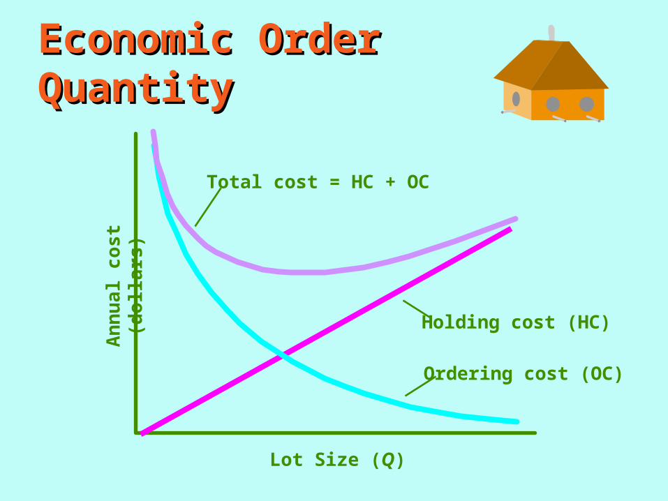
Lot Size (Q)

Ordering cost (OC)

Holding cost (HC)

Total cost = HC + OC

Economic Order QuantityEconomic Order Quantity

| | | | | | | |50 100 150 200 250 300 350 400

An

nu

al c

ost

(d

oll

ars)

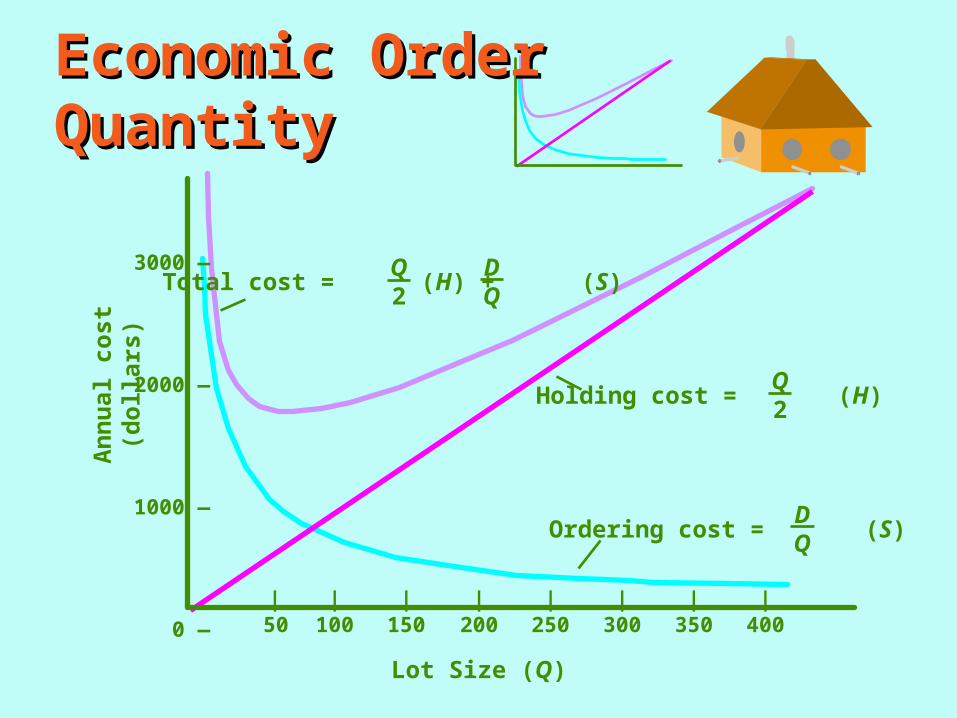
Lot Size (Q)

3000 —

2000 —

1000 —

0 —

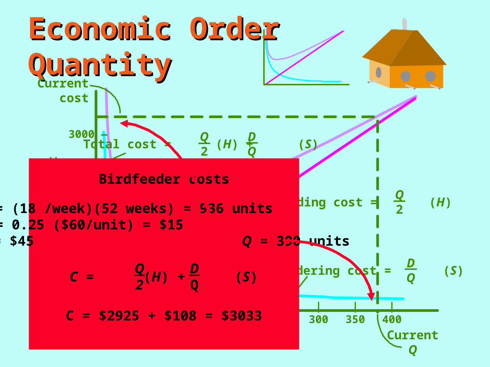
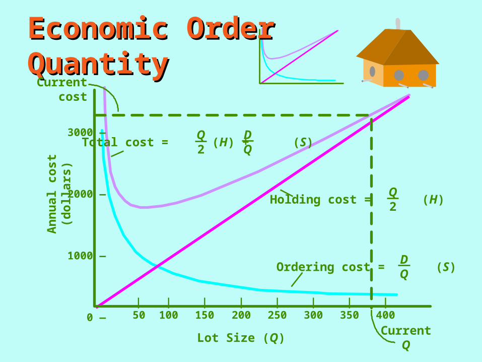
Total cost = (H) + (S)DQ

Q2

Holding cost = (H)Q2

Ordering cost = (S)DQ

Economic Order QuantityEconomic Order QuantityA

nn

ual

co

st (

do

llar

s)

| | | | | | | |50 100 150 200 250 300 350 400

3000 —

2000 —

1000 —

0 —

Total cost = (H) + (S)DQ

Q2

Holding cost = (H)Q2

Ordering cost = (S)DQ

Lot Size (Q)

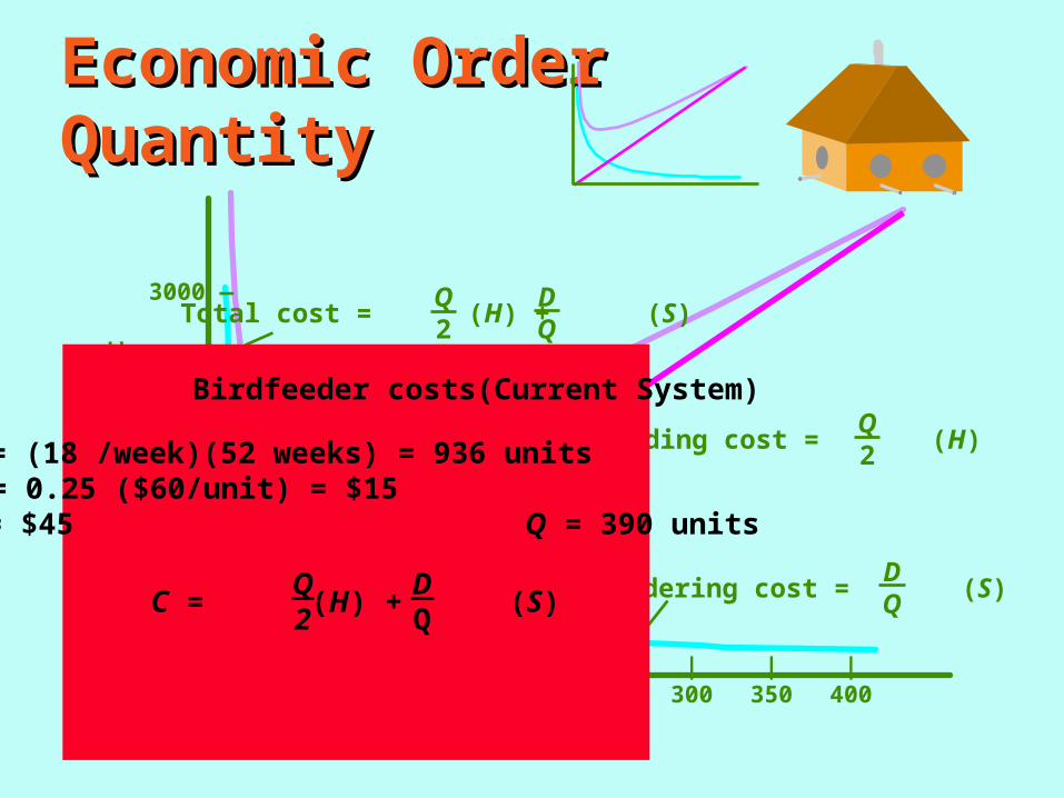
Birdfeeder costs(Current System)

C = (H) + (S)Q2

DQ

D = (18 /week)(52 weeks) = 936 unitsH = 0.25 ($60/unit) = $15S = $45 Q = 390 units

Economic Order QuantityEconomic Order QuantityA

nn

ual

co

st (

do

llar

s)

| | | | | | | |50 100 150 200 250 300 350 400

Lot Size (Q)

3000 —

2000 —

1000 —

0 —

Total cost = (H) + (S)DQ

Q2

Holding cost = (H)Q2

Ordering cost = (S)DQ

Birdfeeder costs (Current System)

C = (H) + (S)Q2

DQ

D = (18 /week)(52 weeks) = 936 unitsH = 0.25 ($60/unit) = $15S = $45 Q = 390 units

C = $2925 + $108 = $3033

Economic Order QuantityEconomic Order Quantity

| | | | | | | |50 100 150 200 250 300 350 400

An

nu

al c

ost

(d

oll

ars)

Lot Size (Q)

3000 —

2000 —

1000 —

0 —

Currentcost

CurrentQ

Total cost = (H) + (S)DQ

Q2

Holding cost = (H)Q2

Ordering cost = (S)DQ

Birdfeeder costs

C = (H) + (S)Q2

DQ

D = (18 /week)(52 weeks) = 936 unitsH = 0.25 ($60/unit) = $15S = $45 Q = 390 units

C = $2925 + $108 = $3033

Economic Order QuantityEconomic Order Quantity

| | | | | | | |50 100 150 200 250 300 350 400

An

nu

al c

ost

(d

oll

ars)

Lot Size (Q)

3000 —

2000 —

1000 —

0 —

Currentcost

CurrentQ

Total cost = (H) + (S)DQ

Q2

Holding cost = (H)Q2

Ordering cost = (S)DQ

Economic Order QuantityEconomic Order Quantity

| | | | | | | |50 100 150 200 250 300 350 400

An

nu

al c

ost

(d

oll

ars)

Lot Size (Q)

3000 —

2000 —

1000 —

0 —

Currentcost

CurrentQ

Total cost = (H) + (S)DQ

Q2

Holding cost = (H)Q2

Ordering cost = (S)DQ

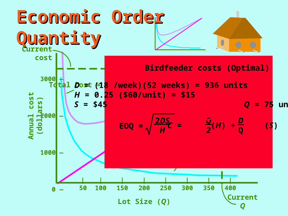
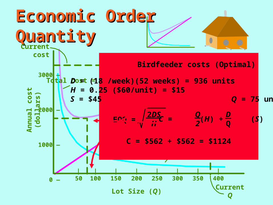
Birdfeeder costs (Optimal)

D = (18 /week)(52 weeks) = 936 unitsH = 0.25 ($60/unit) = $15S = $45 Q = EOQ

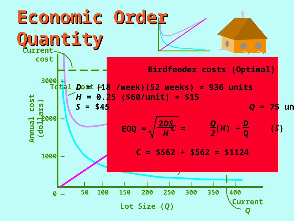
C = (H) + (S)Q2

DQEOQ =

2DSH

Economic Order QuantityEconomic Order Quantity

| | | | | | | |50 100 150 200 250 300 350 400

An

nu

al c

ost

(d

oll

ars)

Lot Size (Q)

3000 —

2000 —

1000 —

0 —

Currentcost

CurrentQ

Total cost = (H) + (S)DQ

Q2

Holding cost = (H)Q2

Ordering cost = (S)DQ

Birdfeeder costs (Optimal)

D = (18 /week)(52 weeks) = 936 unitsH = 0.25 ($60/unit) = $15S = $45 Q = 75 units

C = (H) + (S)Q2

DQEOQ =

2DSH

Economic Order QuantityEconomic Order Quantity

| | | | | | | |50 100 150 200 250 300 350 400

An

nu

al c

ost

(d

oll

ars)

Lot Size (Q)

3000 —

2000 —

1000 —

0 —

Currentcost

CurrentQ

Total cost = (H) + (S)DQ

Q2

Holding cost = (H)Q2

Ordering cost = (S)DQ

Birdfeeder costs (Optimal)

D = (18 /week)(52 weeks) = 936 unitsH = 0.25 ($60/unit) = $15S = $45 Q = 75 units

C = $562 + $562 = $1124

C = (H) + (S)Q2

DQEOQ =

2DSH

Economic Order QuantityEconomic Order Quantity

| | | | | | | |50 100 150 200 250 300 350 400

An

nu

al c

ost

(d

oll

ars)

Lot Size (Q)

3000 —

2000 —

1000 —

0 —

Currentcost

CurrentQ

Total cost = (H) + (S)DQ

Q2

Holding cost = (H)Q2

Ordering cost = (S)DQ

Birdfeeder costs (Optimal)

D = (18 /week)(52 weeks) = 936 unitsH = 0.25 ($60/unit) = $15S = $45 Q = 75 units

C = $562 + $562 = $1124

C = (H) + (S)Q2

DQEOQ =

2DSH

Economic Order QuantityEconomic Order Quantity

| | | | | | | |50 100 150 200 250 300 350 400

An

nu

al c

ost

(d

oll

ars)

Lot Size (Q)

3000 —

2000 —

1000 —

0 —

Currentcost

CurrentQ

Total cost = (H) + (S)DQ

Q2

Holding cost = (H)Q2

Ordering cost = (S)DQ

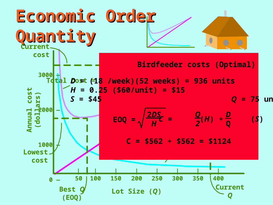
Birdfeeder costs (Optimal)

D = (18 /week)(52 weeks) = 936 unitsH = 0.25 ($60/unit) = $15S = $45 Q = 75 units

C = $562 + $562 = $1124

C = (H) + (S)Q2

DQEOQ =

2DSH

Lowestcost

Best Q(EOQ)

Economic Order QuantityEconomic Order Quantity

| | | | | | | |50 100 150 200 250 300 350 400

An

nu

al c

ost

(d

oll

ars)

Lot Size (Q)

3000 —

2000 —

1000 —

0 —

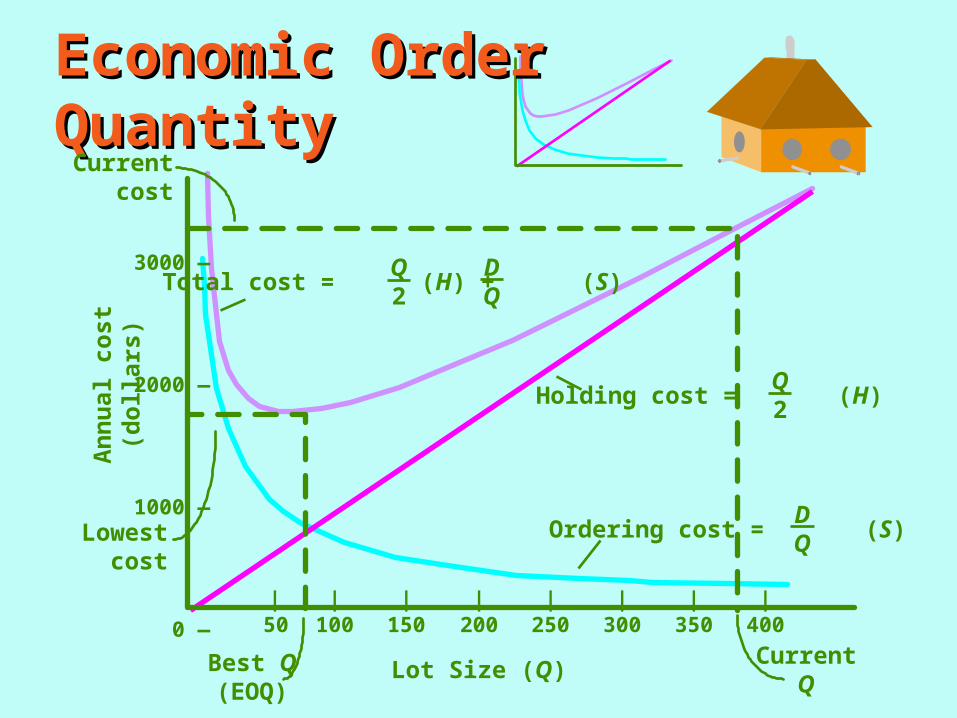
Currentcost

Lowestcost

Best Q(EOQ)

CurrentQ

Total cost = (H) + (S)DQ

Q2

Holding cost = (H)Q2

Ordering cost = (S)DQ

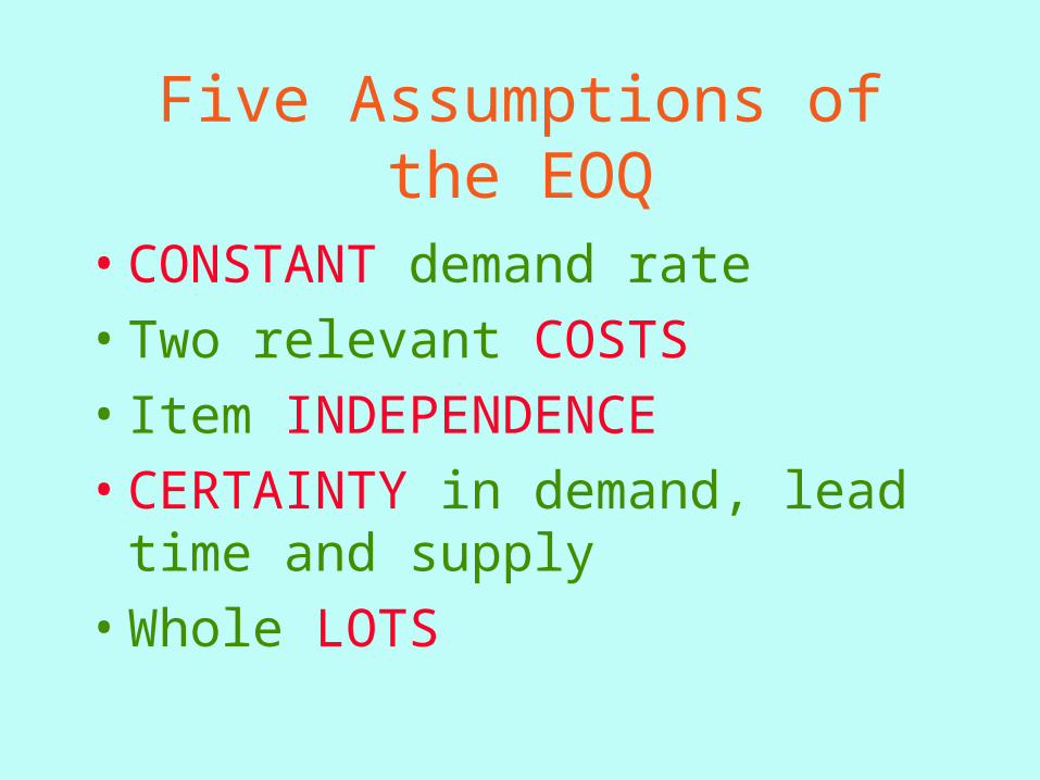
Five Assumptions of the EOQ

• CONSTANT demand rate

• Two relevant COSTS

• Item INDEPENDENCE

• CERTAINTY in demand, lead time and supply

• Whole LOTS

Realistic?• No Way ......

• ................ BUT, since EOQ is relatively insensitive to errors, IT WORKS ANYWAY!

How How Much?Much? When!When!

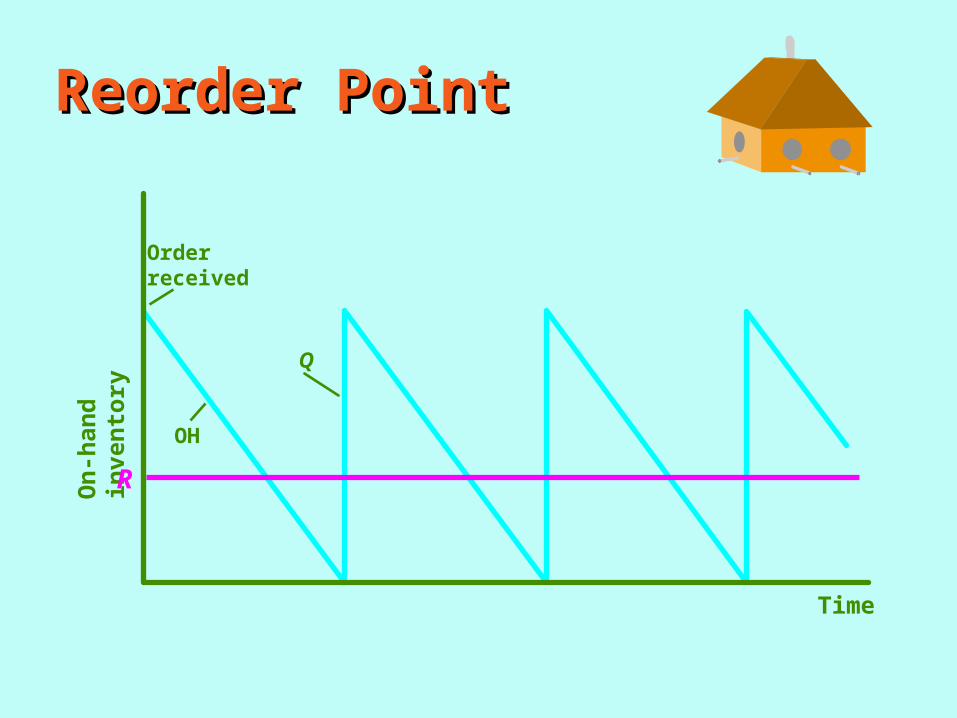
Reorder PointReorder PointO

n-h

and

in

ven

tory

Time

R

Orderreceived

Q

OH

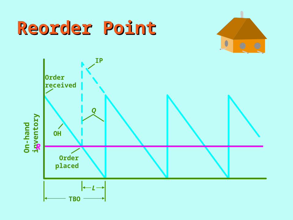
Reorder PointReorder PointO

n-h

and

in

ven

tory

Orderreceived

Q

OH

Orderplaced

IP

TBO

L

R

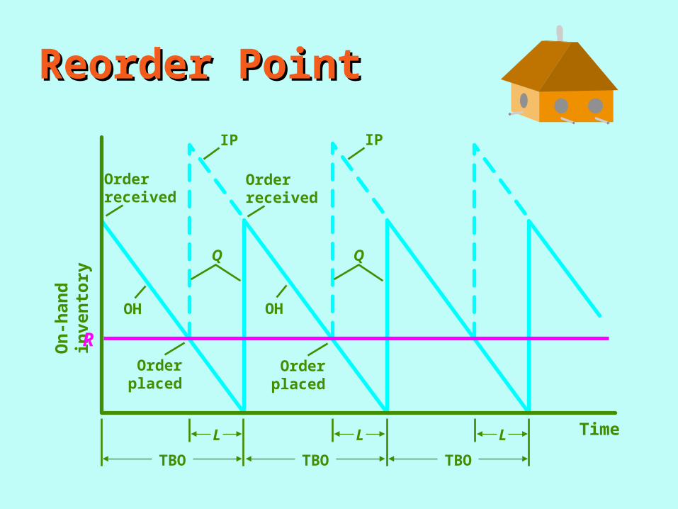
Reorder PointReorder PointO

n-h

and

in

ven

tory

Time

Orderreceived

Orderreceived

Q Q

OH OH

Orderplaced

Orderplaced

IP IP

TBO

L

TBO

L

TBO

L

R

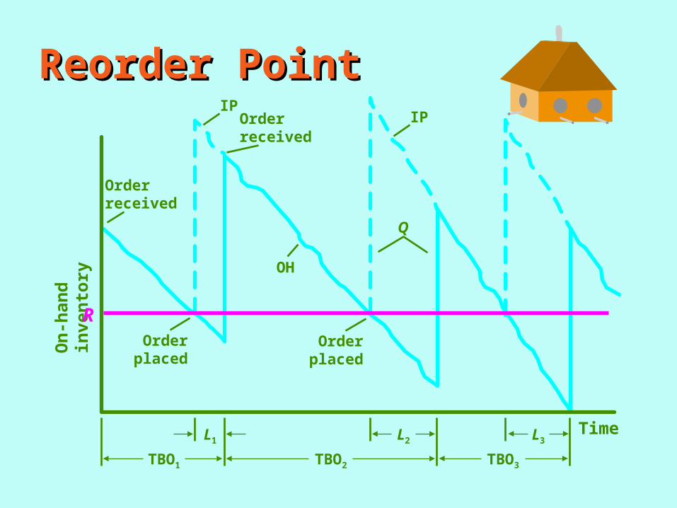
Reorder PointReorder Point

Time

On

-han

d i

nve

nto

ry

Orderreceived

Orderreceived

Q

OH

Orderplaced

Orderplaced

IPIP

R

TBO1 TBO2 TBO3

L1 L2 L3

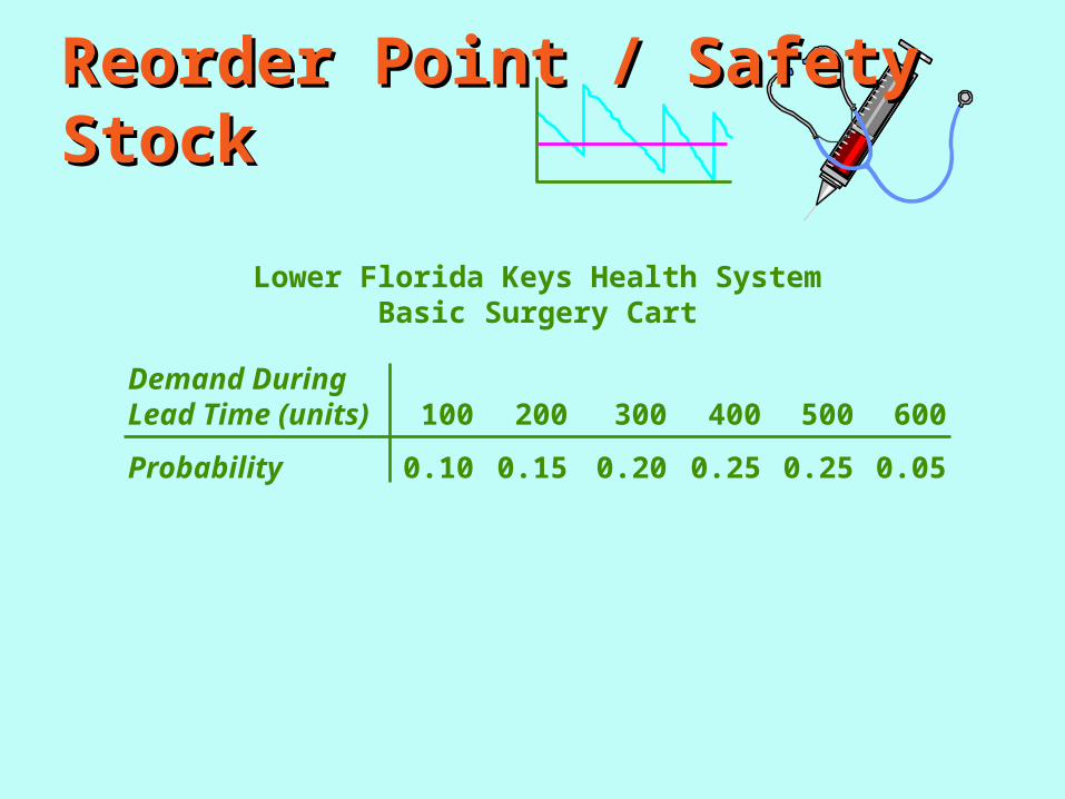
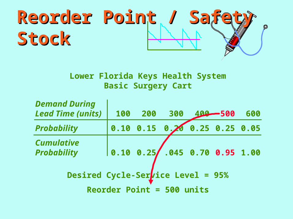
Reorder Point / Safety StockReorder Point / Safety Stock

Lower Florida Keys Health SystemBasic Surgery Cart

Demand DuringLead Time (units) 100 200 300 400 500 600

Probability 0.10 0.15 0.20 0.25 0.25 0.05

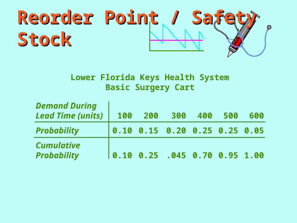
Reorder Point / Safety StockReorder Point / Safety Stock

Lower Florida Keys Health SystemBasic Surgery Cart

Demand DuringLead Time (units) 100 200 300 400 500 600

Probability 0.10 0.15 0.20 0.25 0.25 0.05

CumulativeProbability 0.10 0.25 .045 0.70 0.95 1.00

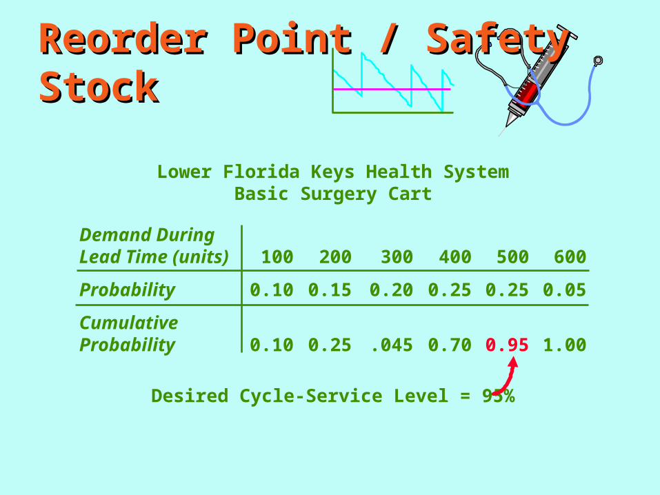
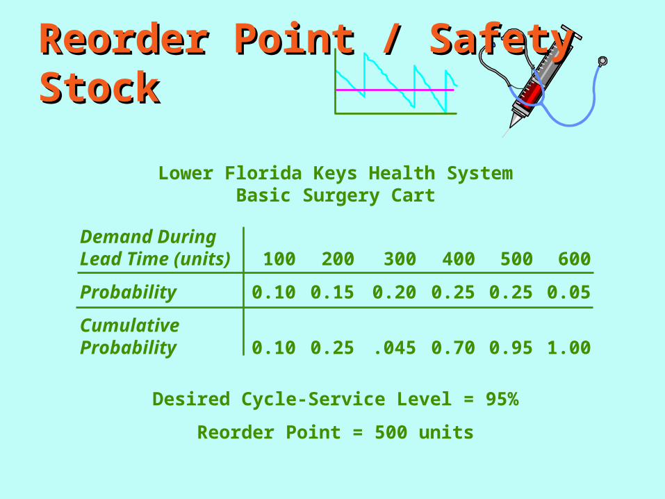
Reorder Point / Safety StockReorder Point / Safety Stock

Lower Florida Keys Health SystemBasic Surgery Cart

Demand DuringLead Time (units) 100 200 300 400 500 600

Probability 0.10 0.15 0.20 0.25 0.25 0.05

CumulativeProbability 0.10 0.25 .045 0.70 0.95 1.00

Desired Cycle-Service Level = 95%

Reorder Point / Safety StockReorder Point / Safety Stock

Lower Florida Keys Health SystemBasic Surgery Cart

Demand DuringLead Time (units) 100 200 300 400 500 600

Probability 0.10 0.15 0.20 0.25 0.25 0.05

CumulativeProbability 0.10 0.25 .045 0.70 0.95 1.00

Desired Cycle-Service Level = 95%

Reorder Point = 500 units

Reorder Point / Safety StockReorder Point / Safety Stock

Lower Florida Keys Health SystemBasic Surgery Cart

Demand DuringLead Time (units) 100 200 300 400 500 600

Probability 0.10 0.15 0.20 0.25 0.25 0.05

CumulativeProbability 0.10 0.25 .045 0.70 0.95 1.00

Desired Cycle-Service Level = 95%

Reorder Point = 500 units

Reorder Point / Safety StockReorder Point / Safety Stock

Lower Florida Keys Health SystemBasic Surgery Cart

Demand DuringLead Time (units) 100 200 300 400 500 600

Probability 0.10 0.15 0.20 0.25 0.25 0.05

CumulativeProbability 0.10 0.25 .045 0.70 0.95 1.00

Desired Cycle-Service Level = 95%

Reorder Point = 500 units

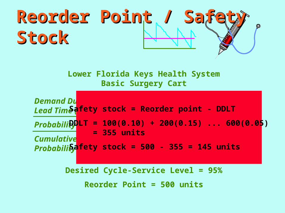
Safety stock = Reorder point - DDLT

DDLT = 100(0.10) + 200(0.15) ... 600(0.05)= 355 units

Safety stock = 500 - 355 = 145 units

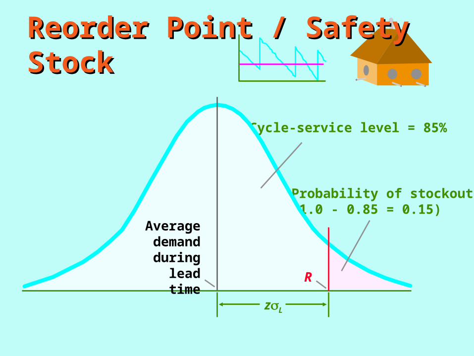
Reorder Point / Safety StockReorder Point / Safety Stock

Probability of stockout(1.0 - 0.85 = 0.15)

Cycle-service level = 85%

Average demand

during lead time

zL

R

Reorder Point / Safety StockReorder Point / Safety Stock

Demand during lead time = 36 units

L = 15 Cycle/service level = 90%

Time

On

-ha

nd

in

ven

toryR

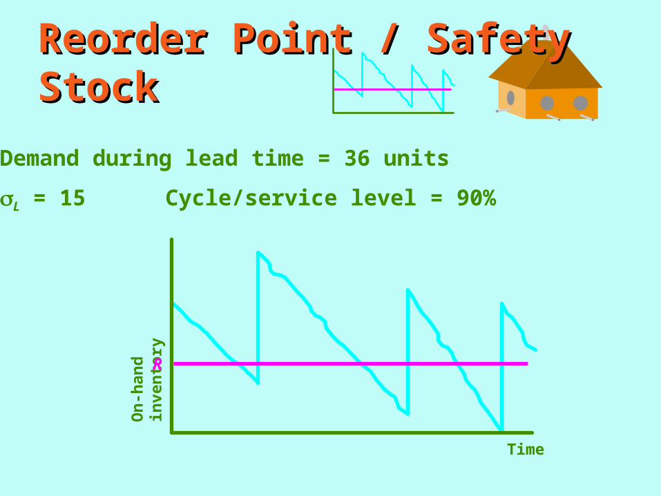
Reorder Point / Safety StockReorder Point / Safety Stock

Demand during lead time = 36 units

L = 15 Cycle/service level = 90%

Time

On

-ha

nd

in

ven

toryR

z = 1.28

Safety stock = zL = 19.2 20

Reorder point = 36 + 20 = 56

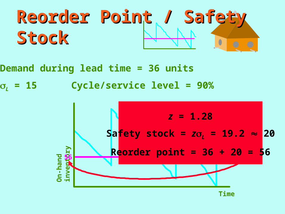
Reorder Point / Safety StockReorder Point / Safety Stock

Demand during lead time = 36 units

L = 15 Cycle/service level = 90%

Time

On

-ha

nd

in

ven

tory56

z = 1.28

Safety stock = zL = 19.2 20

Reorder point = 36 + 20 = 56

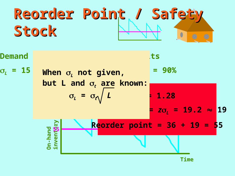
Reorder Point / Safety StockReorder Point / Safety Stock

Demand during lead time = 36 units

L = 15 Cycle/service level = 90%

Time

On

-ha

nd

in

ven

tory55

z = 1.28

Safety stock = zL = 19.2 19

Reorder point = 36 + 19 = 55

When L not given, but L and t are known:

L = t L

Current Practice Papers