Embed Size (px)
Citation preview

Why is Distance Important for Hospital Choice?
Separating Home Bias from Transport Costs∗
Devesh Raval
Federal Trade Commission
Ted Rosenbaum
Federal Trade Commission
February 12, 2019
Abstract
In retail and health care markets, demand declines with geographic distance to the establish-
ment, but either transport costs or preferences correlated with distance (“home bias”) could
cause this decline. Using hospital choices for childbirth, we find that, after controlling for
home bias using fixed effects, estimates of the transport cost disutility fall by 40% relative to
a standard logit model. We show that referrals are a likely source of home bias. Through two
examples – a simulated merger and a planned hospital move – we demonstrate that controlling
for home bias can imply greater substitution between geographically distant hospitals.
∗The views expressed in this article are those of the authors. They do not necessarily represent thoseof the Federal Trade Commission or any of its Commissioners. We thank John Asker, Lorenzo Caliendo,Doireann Fitzgerald, Dan Hosken, Jonathan Heathcote, Tom Holmes, Derek Neal, Ezra Oberfield, NathanPetek, Unni Pillai, Dave Schmidt, Jim Schmitz, Sebastian Sotelo, Brett Wendling, Nathan Wilson, andYoto Yotov for their comments on this paper. We thank Martin Hackmann for discussing this paper at the2018 ASHE Conference, as well as Sebastian Fleitas, Everett Grant, and Massimiliano Piacenza for theirdiscussions of previous versions of the paper. We thank Jonathan Byars and Aaron Keller for their researchassistance.
1

1 Introduction
As economists have known since Hotelling (1929), demand declines rapidly with distance in
retail and health care markets. For example, Gowrisankaran et al. (2015) find that a five
minute increase in travel time to a hospital reduces demand between 17 and 41 percent.
Holmes (2011) finds that an increase in consumer distance to a Wal-Mart from zero to five
miles can decrease demand by 80 percent. In addition, perhaps the most robust empirical
relationship in economics is the gravity equation, which predicts that the distance between
trading partners engaged in international trade is roughly inversely proportional to their
trade flow. In this article, we examine the role of distance in health care markets.
Distance plays an important role in the welfare analysis of health care policies. Hospital
merger evaluation focuses on estimating patients’ willingness to travel to obtain medical
care, which can determine both the likely price effects and the proper antitrust market
definition for a given merger. Optimal design of network adequacy and critical access provider
regulation both depend on how far patients are willing to travel. Patient disutility of travel
is often used as a way to empirically value patient preferences over quality and other hospital
characteristics.
Researchers typically interpret distance effects as due to transport costs. However, as
Doane et al. (2012) note, travel time matters far more relative to hospital quality than would
be expected from the opportunity cost of time. An alternative explanation for distance
effects is that distance is correlated with unobserved consumer preferences, a correlation we
refer to as “home bias”. When distance effects also reflect such differences in preferences,
counterfactual policy analysis will understate consumers’ willingness to travel, distorting
policy conclusions.
We identify the effects of transport costs after accounting for home bias using patient’s
choice of hospital for childbirth.1 Our identification comes from women who move and switch
hospitals between their first two births, so their distance to hospital providers changes over
time. If transport costs are large, women should typically switch to hospitals near their new
1Childbirth is a good context to study this question because the services that the patient needs are similaracross multiple childbirths, but patients do not typically need to return to the same hospital where theypreviously received care.
2

residence. If home bias is large, the change in distance should have a much smaller effect on
their choice.
Formally, we employ a panel data fixed effects approach from Chamberlain (1980). In this
model, we define home bias as patient specific preferences for a hospital that are persistent
over time and larger on average for hospitals that a patient lives close to. We use data
on inpatient childbirths in Florida between 2006 and 2014, and compare our fixed effects
estimates to the common approach in the literature – a logit model using patient choices
that does not control for individual patient-hospital interactions. The disutility of transport
costs derived from the fixed effects estimator falls by about 40% compared to those derived
from the standard logit approach. For example, the standard discrete choice framework
implies that demand falls by 9.7% for a 1 minute increase in travel time for a hospital with a
20% share of the market, compared to a 5.4% fall in demand using the fixed effects estimator.
Thus, without controlling for home bias, one will substantially overestimate the disutility of
transport costs.
We account for a number of possible challenges to the internal and external validity of
our results. One possible concern with our estimates is that the disutility of transport costs
is different for women who move and switch hospitals compared to the full sample of women
giving birth in Florida. However, we find similar estimates for the standard logit estimator for
both datasets. The fixed effects estimator also provides consistent estimates when switching
hospitals is costly for women. In addition, we consider changes in consideration sets post-
move, time-varying unobservables correlated with changes in distance, additional control
variables, and measurement error in distance, and conclude that none of these factors can
explain our findings.
We next find that referral patterns are likely an important determinant of home bias. If
patients’ hospital choices depend on their physicians, physicians’ offices are located near their
patients, and physicians refer to hospitals near their offices, referral networks would magnify
any effect of distance.2 We empirically examine how physician referrals affect our results by
including an indicator variable for hospitals at which patients’ obstetricians practice, and find
2A similar argument applies for a patient’s network of friends. We present a simple model that illustratesthat the social multiplier from peers required to match the gap between our standard logit and fixed effectsestimates is within estimates found in the peer effects literature in other contexts (Glaeser et al., 2003).
3

that doing so explains half of the gap between the standard logit and fixed effect estimates.
In contrast, we do not find evidence that switching costs or catering to local demand can
explain our home bias effects.
We then show that controlling for home bias may change the conclusions of policy analysis
using three applications. Through a simulated hospital merger and planned hospital move,
we show how controlling for home bias can imply greater substitution to a geographically
distant hospital. By estimating patients’ marginal rate of substitution between quality and
distance, we show that patients may be more willing to travel to go to higher quality hospitals.
We first illustrate how accounting for referral patterns, one mechanism for home bias,
affects predicted harm from mergers. We decompose the referral function of Ho and Pakes
(2014a), who show that patient choices respond to physician incentives, and are thus a
function of both physician and patient preferences. We assume that both patients and
clinicians dislike traveling and that patients’ choice of hospitals depends both on their own
and their clinician’s disutility for travel. In this context, the clinician’s disutility for travel
can generate home bias. In a simulation, we replicate our findings that failing to account for
home bias overstates consumers’ disutility of travel. Further, if insurance companies only
care about patient preferences, we find that ignoring home bias understates merger harm
by a magnitude that could lead to permitting a problematic merger. More broadly, our
simulated results thus show that, under realistic parameter values, failing to account for
home bias could lead to inefficient merger policy.
In our second application, we show that evaluations of network adequacy considerations
have to account for home bias effects. We examine a policy evaluation of the proposed
relocation of a Hospital Corporation of America (HCA) hospital opposed by several hospital
systems in a Certificate of Need (CON) filing. A major point of contention was whether
patients living close to the old location, but far from the new location, would be harmed
because they would be unwilling to travel to the new location. The fixed effects estimates
imply that the new hospital would lose a much smaller share of patients that lived far from
the new hospital site but close to the old one compared to the standard logit estimates,
because patients are much more willing to travel under the fixed effects model.3 Thus, the
3In this counterfactual, we assume that patient-hospital interactions remain constant immediately follow-
4

fixed effects model predicts less harm from the move for patients living far from the new
location than the standard logit model.
In addition, our results on home bias affect welfare analyses that use distance as a welfare
metric. For example, Capps et al. (2010) use patient’s disutility for distance to dollar de-
nominate the welfare loss of hospital closures. Gowrisankaran et al. (2017) measure patient’s
valuation of Critical Access Hospitals in Medicare’s Rural Hospital Flexibility Program in
terms of distance. In addition, previous work has used distance to determine patients’ valu-
ation of quality (Romley and Goldman, 2011; Chandra et al., 2016; Gaynor et al., 2016). In
our third application, we recalculate patients’ marginal rate of substitution between quality
and distance and find that patients are more sensitive to hospital quality than previously
thought.
A large literature finds that a consumer’s demand declines with distance for industrial
organization markets, and that consumers’ aversion to travel is critical to understand where
retailers set up stores and how they respond to changes in competition (Holmes (2011),
Houde (2012), Thomadsen (2005)).4 In healthcare markets, distance to medical provider is
one of the most important predictors of provider choice (Capps et al. (2003), Gowrisankaran
et al. (2015), Ho (2006), Raval et al. (2017a)).
Three recent articles demonstrate how distance can affect demand other than through
transport costs in other contexts. In the setting closest to ours, Beckert and Collyer (2017)
find that distance elasticities fall by over 50% after accounting for physician referrals in
a population of UK patients choosing hospitals for elective surgeries. Moraga-Gonzalez et
al. (2017) derive a search model for automobile purchase in which distance affects search
frictions rather than consumer utility. Chaney (2018) develops a model of international
trade in which the social network of entrepreneurs can lead to gravity effects without direct
transportation costs from trade.
This article proceeds as follows. In Section 2, we outline a model of provider choice
ing the move, which could reflect that referral patterns take time to adjust.4In addition, the gravity equation in trade arises naturally out of several economic models (Bergstrand
(1985), Head and Mayer (2013)). Anderson and Van Wincoop (2004) and Anderson (2011) provide surveysof the empirical evidence in international trade. A gravity equation has been documented by Hortacsu et al.(2009) for online commerce, Grogger and Hanson (2011) for migration, Helpman et al. (2004) for FDI, andWolf (2000) for domestic trade.
5

and our approaches to identification. In Section 3, we describe the data. In Section 4, we
estimate the disutility of transport costs. In Section 5, we examine several mechanisms for
home bias. In Section 6, we show the implications of controlling for home bias for three
counterfactual policy applications. We conclude in Section 7.
2 Identification of Consumer Choice Model
We begin by reviewing a workhorse model of a patient’s hospital choice used in many recent
papers as the cornerstone of a broader empirical model of hospital and insurer bargaining
(Capps et al. (2003), Gowrisankaran et al. (2015), Ho and Lee (2017)). We then show how
to use panel data to identify the disutility of transport costs in the presence of home bias.
2.1 Baseline Model
Patient i becomes pregnant at time t in market m. She chooses hospital j from a set of
hospitals H (j = 1, ..., N) that are available to her based on the utility from receiving care
there. She can also choose an outside option j = 0. Patient i’s utility from care at hospital
j at time t is given by:5
uijt = δijt + εijt. (1)
The mean utility of hospital j for patient i at time t is δijt, while εijt is a Type-I extreme
value distributed patient-hospital-time i.i.d error term that reflects a patient’s idiosyncratic
hospital preferences. We normalize the mean utility of the outside option to zero.
A patient’s ex-ante probability of choosing hospital j at time t is given by:
Pr(hit = j) =exp(δijt)∑
k∈0,...,N exp(δikt). (2)
We then parametrize δijt to include distance, switching costs, and observed and unob-
5As Ho and Pakes (2014a) note, a patient’s decision of where to go to the doctor is the result of acombination of preferences of the woman, her physician, and her insurer. In the first sections of this paper,as in Gowrisankaran et al. (2015), Ho and Lee (2017), and other papers in this literature, we give this functiona welfare interpretation. In Section 6, we decompose this function in such a way that some components affectwelfare, but others do not.
6

served components of a patient’s tastes for hospitals:
uijt = αdijt + βxijt + γI[j = Hit−1] + ξij + εijt, (3)
where
Hit−1 = arg maxk=0,...,N
uikt−1.
In equation (3), dijt is the distance from patient i’s residence to hospital j at time t, while
ξij represents persistent patient preferences for a given facility. These persistent preferences
could be the result of persistent doctor or friend referral patterns, patient specific preferences
for hospital amenities, or proximity to another location to which the patient frequently travels
such as a workplace.
Since we focus on young women with childbirths, a fairly clinically homogeneous pop-
ulation, we suppress observable time-varying characteristics xijt in the utility function.6
I[j = Hit−1] is a dummy variable indicating whether the patient visited hospital j on her
previous visit. Therefore, γ represents the switching costs of visiting a different hospital on
different visits.
The semi-elasticity of demand for hospital j with respect to transport costs depends both
upon the transport cost parameter α and hospital j’s share of the market. As a hospital’s
share rises, the effect of transport costs on demand falls. The transport cost semi-elasticity
is the coefficient on distance, α, multiplied by the probability that the patient goes to any
other hospital 1− Pr(hit = j):
d log(Pr(hit = j))
d(dijt)= α(1− Pr(hit = j)). (4)
2.2 Identification
The identification approach used in previous research estimating patient demand for health
care providers typically makes two implicit assumptions (Gowrisankaran et al., 2015; Ho
and Lee, 2017; Ho and Pakes, 2014a; Raval et al., 2017a). First, individual preferences for
6If there is variation over time within individuals in other variables, we could identify β for those charac-teristics as well. For example, see Raval and Rosenbaum (2016) for steering effects of Medicaid MCOs.
7

hospitals only vary with patient observable characteristics, which is equivalent to restrictions
on the form of ξij. Second, switching costs γ are assumed to be zero.7 These two assumptions
have important implications for the interpretation of distance estimates, since they both rule
out the possibility for home bias. Consumer preferences exhibit home bias when unobserved
tastes ξij are, on average, larger for individuals living closer to hospital j.
For consistent estimates of the disutility of transport costs in this framework, unobserv-
able patient preferences for hospitals ξij must be independent of a patient’s distance from
the hospital dijt. For example, given home bias of preferences, logit estimates will overesti-
mate the effect of distance. Further, for patients who do not move residential location, the
patient’s previous choice will also be a function of her distance to the hospital. In that case,
when there are switching costs (so γ > 0), the error term when switching costs are excluded
will be a function of distance dijt and unobserved preferences ξij.
We address these endogeneity issues by using the fixed effects logit approach of Chamber-
lain (1980) to identify the transport cost parameter α. This approach conditions on the sum
of an individual’s choices over time, and identifies the parameters of interest from variation
in the sequence of choices over time.
For intuition, consider Figure 1, which shows a woman who has hospitals A, B, and C
in her choice set for both her first and second birth. For her first birth, she lived closer to
hospital A than hospital B. Between the two births, she moves residences, such that for her
second birth she is closer to hospital B than hospital A. The conditional logit estimator is
based upon the probability that she went to hospital A for the first birth, and then hospital
B for the second birth, compared with the opposite order. Since hospital A is located closer
to her for the first birth, and hospital B is located closer to her for the second birth, her
likelihood of going to A for the first birth and B for the second birth increases as the disutility
of transport costs α rises.
Since both hospitals A and B were options each time, the fixed effects approach differences
out any time-invariant hospital-patient interactions. Switching costs are also differenced out,
because in either case the patient incurs a switching cost γ in the second period. We are
7One recent exception is Shepard (2016), who estimates a demand model which allows for state dependence(i.e., γ 6= 0), although he acknowledges that he is unable to separately identify preference heterogeneity fromstructural state dependence.
8

Figure 1 Identification Intuition
Residence fori’s First Birth
Residence fori’s Second Birth
AFirst Birth
Hospital
BSecond Birth
Hospital
CNo BirthHospital
di1A
di1B
di1C
di2A
di2B
di2C
then able to identify the marginal impact of changing dijt using the conditional likelihood.
Consider women that went to hospital A for one birth and hospital B for the other
birth. Then, if εijt is distributed Type-I extreme value, Chamberlain (1980) shows that the
conditional probability that these women went to A first and B second is a function of the
“difference in difference” in distance: the difference in distance in the second period between
hospital B and hospital A, minus the difference in the first period between hospital B and
hospital A. As the transport cost parameter α gets larger, the probability that the women
went to the hospital that became relatively closer in the second period rises.
Formally, the expression for the conditional probability is:
Pr[(A,B)|(A,B) or (B,A)] =exp(αz)
1 + exp(αz),
where
z = (d2B − d2A)− (d1B − d1A)
and
Pr(j, k) = Pr(hi1 = j, hi2 = k).
Since the ξij terms and switching costs γ are differenced out from the expression, we can
9

consistently estimate α. However, only patients that move residences between their births
and go to different hospitals for each birth provide identifying variation under this approach.8
To see how this identification works, take the choice behavior of the woman in Figure 1.
Let hospital A be ten miles from her residence at first birth, and twenty miles from her
residence at second birth, while hospital B is twenty miles from her residence at first birth
and ten miles from her residence at second birth. In that case, if the transport cost parameter
α is −0.1, her likelihood of going to hospital A for her first birth and then B for the second
birth is 88%. If the transport cost parameter falls by half to −0.05, her likelihood of going
to A first and then B falls to 73%. Thus, the likelihood that she goes to A first and then
B is informative of the degree of disutility of transport costs. Her distance to hospital C
plays no role in this identification approach, as only the hospitals that she went to enter the
conditional likelihood.
2.3 Threats to Identification
Our identification approach assumes that unobserved preferences for hospitals are fixed, and
so only takes account of time-invariant correlations between unobserved patient preferences
for a specific facility and distance. In this section, we examine the implications of potential
time-varying changes in unobserved preference due to patient learning about quality, changes
in patient consideration sets due to the move, and income shocks that affect both patient
location and hospital preference. In general, these threats to our identification strategy will
bias our estimates away from a zero effect of distance.
If patients learn about hospital quality after their hospital visit, the assumption of fixed
unobserved preferences will be violated. While the overall change in hospital quality for the
hospital the patient visited previously across all hospitals and patients will be captured in
the switching costs γ, the update in belief about quality could vary across hospitals and
patients depending on the patient’s experience. However, because our focus is on the role
of distance, our main requirement is that any update to the patient’s belief about hospital
quality is independent of the change in distance from the move, just as the logit error shock
8If patients do not move, it would be impossible under this approach to estimate patients’ travel prefer-ences, since there would be no variation in z.
10

is independent of distance. In our view, this assumption is reasonable.
A second threat to identification is that the hospitals that patients consider when they
make their hospital choice change with the move. In our model, the patient considers both
hospitals in each location; a hospital entering the patient’s consideration set after the move
would have a large increase in the patient-hospital quality ξij, which would break our identi-
fication approach. If consideration sets change such that hospitals that become closer enter
the consideration set, or hospitals that become farther away leave the consideration set, we
will overstate the effect of transport costs. In this scenario, the change in consideration sets
implies that patients move closer to hospitals for which they have a positive preference shock,
and away from hospitals for which they have a negative preference shock, so the change in
distance is negatively correlated with the change in quality. We examine this threat to
identification empirically by comparing small moves to large moves; larger moves are more
likely to change the patients’ consideration set. We find fairly similar estimates for both
types of moves, indicating that major bias in our transport cost coefficients from changes in
consideration set is unlikely.
A third possibility is that a shock both affects a patient’s residence and her hospital
preferences. For example, if a patient has a positive income shock and so both moves to a
more upscale neighborhood and increases her valuation of hospital quality, the fixed effects
estimator will overstate the effects of transport costs so long as higher quality hospitals are
located in more upscale neighborhoods. In order to examine this possible threat to our
identification strategy, we examine only women for whom the difference in zip code median
household income between locations is less than $10,000, and find similar estimates to our
baseline results.
3 Data
We use hospital discharge data obtained from the Florida Agency for Health Care Admin-
istration (AHCA) from 2006 to 2014.9 The data includes the zip code of residence for each
9The limited data set was obtained from the AHCA, but that agency bears no responsibility for anyanalysis, interpretations, or conclusions based on this data.
11

patient, which allows us to compute the travel time from the patients’ residence to each
hospital. Patient identifiers allow us to match births by the same woman over time.
In order to difference out switching costs in our structural estimates, we need to know
the first birth of women in our sample. However, we only have data going back to 2006,
so we do not know of women’s births prior to that date. Because of this initial conditions
problem, we only include women who were at most 21 in 2006. This restriction eliminates
the initial conditions problem for most of the women.10
We report summary statistics in Table I for the full sample of all births in Florida, all
births for women that meet our age restriction, and births for women who meet our age
restriction and contribute to the likelihood of the Chamberlain estimator. The latter set of
women switch both residence and hospital between their first and second birth. Imposing
the age restriction leaves about 35 percent of the women from the full sample of all births in
Florida and about 37 percent of total births. The women in the Chamberlain sample make
up 3.8 percent of the women that meet the age restriction, and their births comprise 5.9
percent of the births of the women that meet the age restriction.
The average age is much higher for the full sample, at 27.6 years, than for the other
datasets that impose the age restriction, all of which have an average age of about 21.7.
As we impose more restrictions, the fraction of admissions that are white falls, from 66
percent for the full sample of births to 52 percent for the Chamberlain dataset, while the
fraction of admissions that are black rises from 23 percent for the full sample to 40 percent
for the Chamberlain dataset. The fraction of admissions that are Hispanic remains constant
at about 20 percent. The fraction of admissions from patients on Medicaid rises from 51
percent for all births, to 72 percent for births of women that meet the age restriction, to 79
percent for the Chamberlain sample. Almost all births are of women living in metropolitan
areas.
We define the choice set for each patient as all hospitals within 45 minutes driving time
of her zip code centroid.11 All hospitals not within this choice set are included together as
the “outside option”. For the Chamberlain sample, we require the hospital chosen for each
10Nationwide, about 87 percent of first births are of mothers age 20 and above and 96 percent of firstbirths are of mothers age 18 or above (Hamilton et al. (2015)).
11See Ho and Pakes (2014a) for a similar choice set restriction.
12

Table I Summary StatisticsAll Age Restriction Chamberlain
Age 27.58 21.73 21.70White 0.66 0.61 0.52Black 0.23 0.30 0.40
Hispanic 0.20 0.20 0.19Medicaid 0.51 0.72 0.79
Metro 0.94 0.92 0.98N Births 1,794,598 667,310 39,462
N Women 1,247,610 439,636 16,718
Note: All datasets are as described in the text.
birth to be in the choice set for both births. This restriction would remove, for example,
women who choose a hospital in Jacksonville at first birth and in Miami at second birth.
Since the data includes the zip code of residence for each patient, the measure of distance
that we use is the travel time from the centroid of the patient’s zip code to each hospital’s
address.12 Figure 2 displays the density for the post-move change in distance for both the
hospital of first birth and hospital of second birth for women in the Chamberlain sample. It
is reassuring that these graphs are close to mirror images of each other; there do not seem
to be systematic differences between changes for the first birth hospital and second birth
hospital. Patients do tend to move closer to their hospital of second birth, and farther away
from their hospital of first birth. On average, the hospital of first birth becomes 3.2 minutes
farther away, and the hospital of second birth becomes 2.7 minutes closer, after the move,
but there is a wide range of changes in distance.
4 Estimates
In this section, we show that fixed effect estimates of the transport cost parameter α are
much lower than estimates from a patient level discrete choice framework that does not
separate unobserved preferences from transport costs.
Using equation (2), we estimate a standard logit model using the disaggregated patient
discharge data that includes hospital indicators and travel time as covariates, but does not
12It is standard to use zip code centroid to calculate distance in hospital choice models; for example, seeGowrisankaran et al. (2015) and Ho and Lee (2017). We use ArcGIS to construct these travel times basedon historic travel time for 8am on Wednesdays.
13

Figure 2 Density of Change in Travel Time after Patient Move for Hospitals of First andSecond Birth
Note: The red line is the smoothed density curve for the change in distance to thehospital of first birth after the patient’s move in residential location between her firstand second birth for the Chamberlain sample; the blue line is the density for the changein distance to the hospital of second birth.
include patient-hospital interactions. We examine these estimates under both the sample
meeting the age restriction and the Chamberlain sample to examine whether the magnitude
of the transport cost coefficient varies between the two populations. While much of the
literature on hospital choice includes more detailed controls for the type of patient, our
sample is extremely homogeneous in that it consists of young women entering the hospital
for the identical procedure. We discuss below a robustness check in which we include a large
set of interactions, and find little change in our estimate of distance.
Figure 3 depicts the absolute value of estimates of α, the transport cost parameter, from
the standard and fixed effect logit models. Both standard logit estimates are of similar
magnitude, with an estimate of -0.121 using the full sample meeting the age restriction and
-0.116 using the Chamberlain sample.13 Thus, for a hospital with a 20% share of the market,
the standard logit estimator predicts a one minute increase in distance will decrease demand
13In our main estimates, we restrict the choice set to only include hospitals within 45 minutes drive timefor each birth. We have conducted a robustness check in which we include all hospitals within 45 minutesdriving time for either birth in the choice set using the Chamberlain sample, so the patients’ choice set doesnot vary over time, and get an estimate of -0.125, similar to our baseline estimates.
14

Figure 3 Estimates of the Transport Cost Coefficient
Note: The standard logit, age restriction sample specification is based on all womenmeeting our age restriction, while the standard logit, Chamberlain sample is based on womenin the “Chamberlain” sample. For each specification, the dot is the point estimate and thelines are the 95% confidence interval. Logit estimates reflect the transport cost parameterα; the semi-elasticity with respect to transport costs is α multiplied by one minus theprobability of going to the hospital. See Table IV for a table of the estimates and standarderrors used to generate this figure.
15

from 9.3 to 9.7%.
The transport costs parameter α from the fixed effects specification is -0.068, approxi-
mately 40% of the standard logit approaches. The fixed effects approach thus implies that
people are much more willing to travel long distances than is implied by the standard logit
approach. As the 95% confidence intervals make clear, the statistical difference between
these coefficients is well beyond that which can be explained by sampling variation.
To demonstrate how our identification approach works, we show how the conditional
choice probability of women choosing a given sequence of hospitals varies with the double
difference in distance, as this relationship is the conditional probability used in the fixed
effects estimator. Since it is arbitrary which conditional probability is used (i.e., which
hospitals are “A” and “B” in Section 2.2), we randomize which hospital is labeled A and B
and display the conditional probability that B is chosen second.
The red line in Figure 4 is the nonparametric relationship between the conditional prob-
ability and the double difference in distance for the women in the Chamberlain sample. The
blue points in the figure represent the implied conditional probabilities using the distance
estimates from the standard logit model estimated on all women meeting the age restriction.
Thus, Figure 4 illustrates the difference between the standard and fixed effect logit estimates.
The nonparametric estimates of the conditional probability decline much less steeply with
distance, which implies a much lower disutility from transport costs.
Our results remain robust to a variety of alternative specifications that relax some of
the assumptions of our model. Our baseline model assumes that all patients have the same
ex-ante treatment complexity, that all patients can visit both hospitals in both periods,
that we observe all births of the women, that there is no time-varying patient/provider
unobservable correlated with the change in distance, and that there is no measurement error
in our estimate of distance.
Our main standard logit specification only includes travel time and hospital fixed effects.
We examine whether including additional interactions would control for home bias in distance
estimates by generalizing the choice models used in Ho (2006) and Gowrisankaran et al.
(2015) through the inclusion of interactions of hospital indicators with whether the delivery
was vaginal or C-section (to account for severity of procedure), whether the delivery was
16

Figure 4 Distance and Conditional Probability of Choice
Note: The red line depicts the nonparametric relationship between the con-ditional probability and the double difference in distance, and the shading the95% confidence interval around this relationship, while the blue points de-pict the implied probabilities under the standard logit model estimated on allwomen meeting the age restriction.
term or pre-term, zip code median income of the patient, and whether the patient was on
commercial insurance.14 Using normal deliveries for the Age Restriction sample, we estimate
a distance coefficient of −0.126, compared to −0.122 without the interactions, so additional
interactions of observed patient and hospital characteristics cannot account for home bias
effects.
To address the concern that patients may vary in treatment complexity, we restrict our
attention to women that had a normal labor and delivery. We also examine normal vaginal
and normal C-section births separately, as well as full term births separately. To address the
concern that some women may have had births prior to 2006, the start of our dataset, we
further restrict our sample to women who were 18 and under in 2006. To address concerns
about heterogeneity across different patient populations, we examine commercial patients
separately, as most of the women in the sample are on Medicaid. While we estimate the
14The models in Ho (2006) and Gowrisankaran et al. (2015) also include interactions with teaching hospitalstatus and other variables that are subsumed within hospital fixed effect interactions, as well as interactionsirrelevant for obstetrics and interactions with travel time which measure heterogeneous effects of travel time.
17

fixed effects model on different subsamples, we recognize that the patient population in these
subsamples is still younger and possibly poorer than the population as a whole.
We also examine multiple reasons that a time-varying patient/hospital unobservable could
arise. Women could shift delivery physician after the move to one closer to her new home,
which could change her preferences for each hospital because the new doctor has different
preferences over hospitals for delivery than the previous doctor. We thus estimate a speci-
fication where we only include women who have the same delivery physician for each birth.
We also examine only women for whom the difference in median household income between
zipcodes is less than $10,000, in order to avoid women who might experience a large income
or other preference shock between births. Finally, in order to examine concerns of changes
in consideration set, we estimate our specifications separately for women with moves less
than and greater than 15 minutes. Inference using smaller moves should be less prone to
bias from changes in consideration sets over time.
Figure 5 depicts the results from these alternate specifications.15 While there is some
variation around our main coefficient estimates, in general the estimates of transport costs
are close to the estimates from the baseline fixed effects approach, and much lower than the
estimates from the standard logit. The only major deviation is for the same clinician speci-
fication for transport costs, for which the transport cost coefficient is -0.04, about 40% lower
than the baseline fixed effects estimate. While the coefficient for the same clinician spec-
ification is measured with considerable error, the estimate is consistent with time-varying
unobservables causing the Chamberlain estimator to overstate transport costs. These ro-
bustness checks thus reinforce the paper’s main message: approaches that do not control for
home bias will overestimate the disutility of transport costs.
In order to ensure that mismeasurement of patient travel time is not driving our results,
we conduct an additional robustness check. Since we only have data on patients’ location
at the zip code level, we examine patients in the Chamberlain sample and construct a
distribution of potential travel times by drawing a travel time for each patient from all
census blocks in the zip codes that she lived in. We then randomly draw a travel time from
15Figure 12 in Appendix D examines several of these same specifications using the standard logit estimator,and finds similar point estimates to the baseline estimates.
18

Figure 5 Robustness Checks for Estimates of the Transport Cost Coefficient
Note: The red lines are the coefficient estimates from the standard logit model whilethe blue lines are the coefficient estimates from the fixed effects model. The solid linesare the point estimates while the dashed lines are the 95% confidence interval. Theblack horizontal lines are the coefficient estimates from our robustness checks. The dotis the point estimate and the lines are the 95% confidence interval. Logit estimatesreflect the transport cost parameter α; the semi-elasticity with respect to transportcosts is α multiplied by one minus the probability of going to the hospital. See Table Vfor a table of the estimates and standard errors used to generate this figure.
19

this sample of travel times for each patient, and randomly draw a sequence of hospital choices
from the conditional likelihood given that the fixed effect estimate of distance is the truth.
We then reestimate our model for these patients using the mismeasured zip code centroids.
This Monte Carlo simulation thus allows us to examine how much the distance coefficient
would change for the fixed effect estimates due to mismeasurement of distance.
We conduct this exercise for the Jacksonville metro area; as Figure 5 demonstrates, the
Chamberlain estimate for Jacksonville is similar to that for the overall sample. Figure 6 plots
the distribution of transport cost coefficients from this exercise, which is shifted slightly to the
right of the “true” value, with the modal value implying a small amount of mismeasurement
of about 0.006, or 9 percent of the fixed effects estimate. This amount of mismeasurement
is much smaller than the difference between the fixed effect and standard logit estimates
in Figure 3. Thus, the probability that more precise data on location would overturn our
results is extremely small.
5 Mechanisms
We now explore three possible drivers for home bias: switching costs, hospitals’ catering to
local demand, and referrals from physicians or peers. All of these mechanisms could increase
demand for nearby hospitals, and so bias the transport cost coefficient. We then examine
whether the estimated effect of distance falls after controlling for these mechanisms for home
bias by estimating the standard logit model after including different proxy variables for home
bias confounders on the Age Restriction sample. We present these results in Figure 7 across
different specifications, together with the estimates for the standard logit and fixed effects
models from Section 4 in red and blue respectively. We find evidence that referrals are a
likely mechanism for home bias.
5.1 Switching Costs
One possible source of home bias is the presence of switching costs from switching from one
hospital to another between births. These switching costs could be pecuniary, such as record
switching, or non-pecuniary, such as the need to acclimate to a new medical facility. We
20

Figure 6 Monte Carlo of Transport Cost Coefficients for Jacksonville Metro Area
Note: The red solid and dashed lines are the point estimate and 95% confidence intervalsfor the standard logit estimate of the distance coefficient for the Jacksonville metro area,while the blue solid and dashed lines are the point estimate and 95% confidence intervalsfor the Chamberlain estimate of the distance coefficient for the Jacksonville metro area.The density curve is based on 1000 estimates of the fixed effects logit model using zip codecentroids as data and random draws from the census block - hospital travel time distributionas the truth.
21

examine the switching cost explanation through two specifications.
First, switching costs should only affect our estimates for births after a woman’s first
birth. Therefore, we reestimate our standard logit specification using only women’s first
births to test whether switching costs drive the lower estimate of transport costs in the fixed
effects estimator. If switching costs are a main driver of home bias, we should expect to see
a lower coefficient on transport costs for women’s first births.
In addition, we include a specification where we explicitly include switching costs. In
Raval and Rosenbaum (forthcoming), we structurally estimate switching costs using a panel
data estimator from Honore and Kyriazidou (2000) and information on the third births of
women in the Chamberlain sample. For this paper, we use that estimate of switching costs
to reestimate a standard logit model including a switching cost parameter.
These results, in Figure 7, show that the distance coefficients for first births (“First
Birth”), and for all births including a calibrated switching cost parameter (“Switching
Cost”), are nearly identical to the distance coefficient in our baseline standard logit specifi-
cation. Therefore, we find little evidence that switching costs are a major factor for home
bias in this context.
5.2 Catering to Local Demand
Another reason why patients could prefer to visit hospitals located nearby them is that
hospitals set their quality to cater to local demand preferences. Health care providers can
cater to local demand in a number of ways. First, hospitals could invest in specialty centers
that match the needs of the local patient population (Devers et al. (2003)). In the case
of obstetrics, for example, hospitals could build or expand labor and delivery rooms and
neo-natal intensive care units, or improve their obstetrics facilities, if the local population
around them values these attributes. Second, many hospitals are affiliated with a religious
denomination – one in six patients in the US are treated by a Catholic hospital alone. While
there is considerable evidence from the older literature on patient choice that patients are
more likely to go to a hospital that shares their religious denomination (Schiller and Levin
(1988)), it is unclear whether patients still consider the religious affiliation of a hospital. If
religiously affiliated hospitals are more likely to be located in neighborhoods whose residents
22

Figure 7 Potential Mechanisms for Home Bias
Note: The red lines are the coefficient estimates from the standard logit model whilethe blue lines are the coefficient estimates from the fixed effects model. The solid linesare the point estimates while the dashed lines are the 95% confidence interval. The blackhorizontal lines are the coefficient estimates from our robustness checks. The dot is the pointestimate and the lines are the 95% confidence interval. Logit estimates reflect the transportcost parameter α; the semi-elasticity with respect to transport costs is α multiplied by oneminus the probability of going to the hospital. See Table VII, Table VIII, and Table IXfor tables of the estimates and standard errors used to generate this figure for the Referral,Switching Cost, and Catering to Local Demand mechanisms.
share their religious affiliation, then local demand based on religious preferences would be
correlated with hospital distance. Third, the medical literature has documented that patients
are more likely to select physicians that share their race, ethnicity, or language (Saha et
al. (2000)). Thus, hospitals could cater to local demand by employing physicians that have
similar demographic characteristics to their patient population, or investing in services valued
by those demographics, such as Spanish language translation services.
We examine the hypothesis of hospitals catering to local demand in three ways. We first
examine whether interactions between hospital religious affiliation and patients’ religious
beliefs affect the distance coefficient. To do so, we include interactions between whether a
zip code has a Catholic school, a proxy for the Catholic proportion of the neighborhood,
23

and whether a hospital is affiliated with the Catholic Church. Second, we examine whether
Hispanics are more likely to go to hospitals with greater Spanish language proficiency. We
thus add interactions between whether the patient is Hispanic and the fraction of obste-
tricians with admitting privileges at the hospital that speak Spanish. Third, to examine
catering to local demand for labor and delivery rooms, we include an interaction between
zip code median income and whether the hospital has a labor and delivery room.16 Figure 7
contains the results from these three specifications as “Catholic”, “Spanish”, and “Birth
Room”, respectively. Since the estimates from all three specifications remain close to our
baseline standard logit estimates, we find very little evidence that catering to local demand
can explain much of the home bias that we document.
5.3 Referrals
5.3.1 Clinician Referrals
Clinician referrals could create home bias because patients choose clinicians that are near
their residence and rely on their referral to determine the hospital they go to, and clinicians
admit patients at hospitals near their offices. The literature has found that clinicians have
an important role in helping patients decide which hospital to go to. For example, Ho and
Pakes (2014a) find that physician incentive payments can affect patients’ choice of hospital
for labor and delivery, while Burns and Wholey (1992) shows that the distance from an
admitting physician’s office to a hospital is a larger factor in hospital choice than the distance
from a patient’s residence to the hospital. In the context of elective surgeries, Beckert and
Collyer (2017) find that the distance from a physician’s office is an important determinant of
hospital choice for patients and that, after accounting for this distance, patients’ estimated
distance elasticity for their hospital choice falls by over 50%.
We test the possibility that clinician preferences for hospitals, or admitting privileges,
drive our results by including binary variables in our standard logit specification based on the
hospitals that the operating clinician practices at. We first include either whether a clinician
16We obtain data on Catholic Schools from http://www.floridaschoolchoice.org/information/
privateschooldirectory/DownloadExcelFile.aspx (downloaded on 12/16/16) and physician languageproficiency from the Florida State Hospital Licensure Database.
24

delivers an average of more than one baby per week at a hospital in that year (“Clinician
Week”), or whether a clinician delivers an average of more than one baby per month at a
hospital in that year (“Clinician Month”). However, if patients first choose their hospital
and then their doctor, these specifications can mechanically explain choices. Thus, we also
include a third specification: looking only at second births, whether the operating clinician
for the first birth delivers an average of more than one baby per month at a hospital in that
year (“Clinician First Birth”). If home bias primarily operates through clinician referrals,
these variables should control for that – leading to a coefficient on distance more similar to
that in the fixed effects specification.
Our results, in Figure 7, show that the distance coefficient falls substantially in these
specifications, explaining about half of the gap between our fixed effects and standard logit
estimates. Thus, clinician referrals are likely important in explaining some, but not all,
of the correlation between distance and unobserved patient preferences for facilities. These
results are consistent with our findings earlier that conditioning on women who had the same
attending clinician for both her first and second birth sharply lowers the estimated distance
coefficient.
5.3.2 Peer Referrals
In addition, social networks could magnify the effect of transportation costs because patients
rely on recommendations from friends and family located close to them. When building a
model of patient choice, Satterthwaite (1985), for example, states that “consumers when
they are seeking a new physician who fits their idiosyncratic needs generally rely on the
recommendations of trusted relatives, friends, and associates.” Hoerger and Howard (1995)
study patient choice of prenatal care physician and find that 51% report using a friend or
colleague as a source of information, and 27% a relative. Harris (2003) also find that 51% of
patients report using family and friends as a source of information to choose their physician.
Recommendations from family and friends can magnify the role of distance if they are
located near the patients’ own location. Goldenberg and Levy (2009) and Backstrom et
al. (2010) both find using data on Facebook friends that the likelihood of being someone’s
Facebook friend is decreasing in distance. In addition, friends that live close by may have a
25
greater influence on a patient’s decisions.
We develop a simple social network model of patient choice based on the economic lit-
erature on social multiplier effects (Glaeser et al., 2003), which has found substantial peer
effects in several settings (Sacerdote, 2011). Appendix B details the model; a patient’s utility
from each hospital depends upon both physical distance and the average of all of her friends’
utilities for the hospitals. This model reduces to one in which her utility for a hospital is
based both upon her distance to the hospital as well as her friends’ average distance to the
hospital. If all of her friends live at the same location as the patient, then the full effect of
distance is a combination of the patient’s own disutility of distance and the weight that she
places on her friends’ utility. If her friends do not all live at the same location, the correlation
between her distance between two hospitals and her friends’ average distance between the
two hospitals also matters; when her friends’ distances are less correlated with her distances,
the multiplier effect of the social network falls.
A social multiplier can plausibly explain much of the difference between the standard
and fixed effect logit estimates. If all of the difference between the standard and fixed
effect logit estimates of distance reflects a social multiplier, the social multiplier would be
2 in the context of our model. The social multiplier literature has found multipliers of
similar magnitude for fraternity and sorority membership based on random assignment of
Dartmouth undergraduate roommates, as well as for schooling and earnings from local area
effects (Glaeser et al., 2003).
6 Applications
In this section, we examine three applications of our estimates of distance effects that show
how accounting for home bias affects policy counterfactuals. In the first application, we
examine a simulated hospital merger and show how accounting for referral patterns, one
possible source of home bias, can affect both estimates of patients’ willingness to travel and
merger harm. In the second application, we analyze a hospital after its repositioning through
a contentious planned move, and show that our fixed effects estimates imply much greater
demand for the relocated hospital in areas close to the old location, but farther from the new
26

location. In the third application, we take an example of using distance as a welfare metric,
and show that accounting for home bias implies that patients are substantially more willing
to travel to receive higher quality care.
6.1 Hospital Merger Analysis
A main area of focus in the academic and legal analysis of hospital mergers has been patient’s
willingness to travel to obtain medical care. In particular, market definition has been critical
in courts’ rulings on FTC challenges of hospital mergers (Capps, 2014; Gaynor and Pflum,
2017). Farther hospitals are more likely to be substitutes for patients at the time they need
medical care when patients are willing to travel farther. Therefore, patients’ willingness to
travel can determine both the likely price effects of a merger and the proper market definition
to analyze it.
In Section 5, we showed evidence that the estimates of patients’ disutility of travel to
obtain medical care falls after accounting for the home bias generated by physician referral
patterns. In this section, we build a stylized model that illustrates how accounting for
referral patterns affects estimates of patients’ willingness to travel and the estimated harm
from mergers. Provided that patients suffer more disutility from travelling to their doctor
than their hospital and that physicians are more likely to refer to hospitals close to them,
we can replicate our findings that controlling for home bias reduces the estimated distance
coefficient. In addition, hospitals located relatively far away from each other are closer
substitutes for patients, which increases estimates of harm from a merger of such hospitals.
6.1.1 Model
Patients are uniformly distributed over a line and can choose between three hospitals and
two clinicians. Hospitals A and C are located at either end of the line, while hospital B is
in the middle. Clinician 1 is located halfway between A and B, while clinician 2 is halfway
between B and C. A diagram is in Figure 8.
We consider a hypothetical merger of hospital A and hospital C, both of which are marked
in bold in the figure. The other hospitals and clinicians are assumed to be independently
27

Figure 8 Market Environment for Simulation
A B C
1 2
owned. While clinicians are assumed to have privileges in all of the hospitals, they refer
more patients to the two hospitals that are closest to them. Therefore, clinician 1 dispropor-
tionately refers to hospitals A and B and clinician 2 disproportionately refers to hospitals B
and C.
Patients first choose a clinician and then a hospital.17 A patient i’s choice of clinician c
reflects her utility for that clinician,
uic = αcdic + εic, (5)
where dic is the distance from the patient to the clinician and εic is an iid logit error draw.
We then decompose the notion of a referral function (Ho and Pakes (2014b)). The referral
function drives choices, but is a combination of the preferences of a patient and a doctor
and so does not represent the patient’s utility function.18 Conditional on choosing clinician
c, patient i’s referral function for hospital h is given by:
rih|c = αhdih + εih︸ ︷︷ ︸uih
+ρdch, (6)
where dih is the distance from the patient to the hospital, εih is an iid logit error draw, and
dch is the distance from the clinician to the hospital.
Summarizing, the three main parameters in this model are:
1. patients’ disutility of travel to hospitals αh,
2. patients’ disutility of travel to doctors αc,
3. doctors’ disutility of travel to hospitals ρ.
17There is no outside option, so all patients choose both a doctor and a hospital.18A consideration set approach, where doctors choose the consideration set and patients choose from that
set, has also been used to model this joint decision problem (Gaynor et al., 2016; Beckert and Collyer, 2017).
28
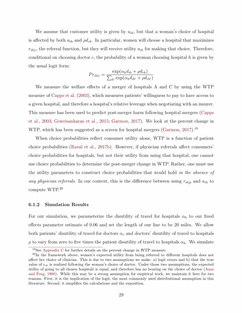
We assume that customer utility is given by uih, but that a woman’s choice of hospital
is affected by both uih and ρdch. In particular, women will choose a hospital that maximizes
rih|c, the referral function, but they will receive utility uih for making that choice. Therefore,
conditional on choosing doctor c, the probability of a woman choosing hospital h is given by
the usual logit form:
Prih|c =exp(αhdih + ρdch)∑h′ exp(αhdih′ + ρdch′)
We measure the welfare effects of a merger of hospitals A and C by using the WTP
measure of Capps et al. (2003), which measures patients’ willingness to pay to have access to
a given hospital, and therefore a hospital’s relative leverage when negotiating with an insurer.
This measure has been used to predict post-merger harm following hospital mergers (Capps
et al., 2003; Gowrisankaran et al., 2015; Garmon, 2017). We look at the percent change in
WTP, which has been suggested as a screen for hospital mergers (Garmon, 2017).19
When choice probabilities reflect consumer utility alone, WTP is a function of patient
choice probabilities (Raval et al., 2017b). However, if physician referrals affect consumers’
choice probabilities for hospitals, but not their utility from using that hospital, one cannot
use choice probabilities to determine the post-merger change in WTP. Rather, one must use
the utility parameters to construct choice probabilities that would hold in the absence of
any physician referrals. In our context, this is the difference between using rih|p and uih to
compute WTP.20
6.1.2 Simulation Results
For our simulation, we parameterize the disutility of travel for hospitals αh to our fixed
effects parameter estimate of 0.06 and set the length of our line to be 20 miles. We allow
both patients’ disutility of travel for doctors αc and doctors’ disutility of travel to hospitals
ρ to vary from zero to five times the patient disutility of travel to hospitals αh. We simulate
19See Appendix C for further details on the percent change in WTP measure.20In the framework above, women’s expected utility from being referred to different hospitals does not
affect her choice of clinician. This is due to two assumptions we make: a) logit errors and b) that the truevalue of εih is realized following the woman’s choice of doctor. Under those two assumptions, the expectedutility of going to all chosen hospitals is equal, and therefore has no bearing on the choice of doctor (Anasand Feng, 1988). While this may be a strong assumption for empirical work, we maintain it here for tworeasons. First, it is the implication of the logit, the most commonly used distributional assumption in thisliterature. Second, it simplifies the calculations and the exposition.
29

10 different datasets of 10,000 patients for each of the parameterizations we consider, and
average across simulations.
In Figure 9, we depict the estimated disutility of travel to a hospital estimated from a
logit model that only includes distance to the hospital as a covariate, which is analogous to
the standard logit model discussed earlier in the paper. The true disutility of travel is shown
as a black horizontal line and the standard logit estimate estimated from the Florida data
is shown as a dashed line. We show the estimated patient disutility of travel to the hospital
as a function of patients’ disutility of travel to doctors αc, shown on the x-axis, and doctors’
disutility of travel to hospitals ρ, shown in the different colors, both in multiples of the true
patient disutility of travel to hospitals.
Patient disutility of travel to a hospital is overstated by a standard logit model when
patients have greater disutility to travel to a doctor than a hospital. The magnitude of this
effect increases in the doctor’s disutility from traveling to hospitals. Since the colored lines
intersect with the dashed line, physician referral effects could generate the magnitude of the
bias that we observe in the data.
In Figure 10, we depict the percent change in WTP from the standard approach that
ignores physician referrals; the black horizontal line is the true percent change in WTP,
which we have set to 25%. As Figure 9 shows, the bias in the distance coefficient can be
obtained by a variety of different parameterizations, so we bold each line in areas that reflect
parameterizations consistent with the bias that we observe in the data. In those areas, the
estimated WTP from the standard approach ranges from 12% - 14%, and thus understates
the estimated harm from the simulated merger. The standard approach overstates competi-
tion between the middle and corner hospitals, and understates the competition between the
corner hospitals. In the absence of a referral, the farthest hospital would be many patients’
second choice, if either of the closer ones became unavailable. However, due to the referrals,
many fewer people go there than if people were making choices purely on the basis of their
own welfare. Therefore, in this case, the competitive effects of the merger are understated.
We map these percent changes in WTP to hospital prices using the estimated elasticity
of 0.2 between WTP and hospital prices of Garmon (2017).21 Given this elasticity, we find
21We use his estimates from a set of 16 hospital mergers that did not have variable cost savings.
30

Figure 9 Estimated Disutility of Travel to Hospital from Simulations
Note: The estimated patient disutility of travel to the hospital from a standard logit model is onthe y-axis, and is shown as a function of patients’ disutility of travel to doctors αc, shown on thex-axis, and doctors’ disutility of travel to hospitals ρ, shown in the different colors, both of whichare expressed in multiples of the true patient disutility of travel to hospitals. The true disutility oftravel is shown as a black horizontal line and the standard logit estimate estimated from the Floridadata is shown as a dashed line.
that a merger of distant hospitals would lead to a predicted price increase of approximately
5% under the true model, but only 2-2.5% under the standard logit model. If a 5% price
threshold for a merger screen is being used, as has been contemplated in other literature
(Miller et al., 2017; Balan and Brand, 2018), using a standard logit model could lead to
incorrectly permitting a problematic merger.22
Our simulations show that in order to measure mergers’ effect on welfare, it can be
important to recover patients’ willingness to travel unconfounded by referral patterns. When
physician referrals play an important role in predicting hospital choice, the only way to
measure patient welfare is to estimate patient preferences, including patients’ true willingness
22Garmon (2017) recommends a threshold of a 6% change in willingness to pay in order to flag problematicmergers, which is different than what we use here. Our point is not to advocate a specific threshold, butrather to show how policy decisions can change as a result of not accounting for referrals in one’s estimationprocedure.
31

Figure 10 Percent Change in WTP Following Simulated Merger
Note: The percent change in WTP from a merger of the two corner hospitals based on thedistance coefficient from a standard logit model is depicted on the y-axis, and is shown as a functionof patients’ disutility of travel to doctors αc, shown on the x-axis, and doctors’ disutility of travel tohospitals ρ, shown in the different colors, both of which are expressed in multiples of the true patientdisutility of travel to hospitals. We bold each line in areas that reflect parameterizations consistentwith the bias in the transport cost coefficient that we observe in the data. The black horizontal lineis the true percent change in WTP, which we have set to 25%.
32

to travel to the hospital. While our conclusions about the direction of bias in welfare effects
are specific to our stylized setting, our results show that it is potentially important to consider
the extent to which this is an issue in a given merger.23
In this simulation, we considered a case where the doctor referral preferences are fixed
before and after the merger. However, if physician practices are owned by merging hospitals
it is possible that the referral patterns of the merging hospitals would change following a
merger.24 Baker et al. (2016) show physician practices owned by a hospital are much more
likely to refer to the hospital that owns them. Therefore, when hospitals own local physician
practices, it may be important in merger analysis to separately identify the distance and
referral parameters and to modify the referral parameter to reflect the change in ownership.
6.2 Network Adequacy: A Planned Hospital Move
In this section, we examine network adequacy through a controversial planned move of
a hospital evaluated by the state regulator. With the move, the hospital moved farther
away from a minority, indigent patient population, and opposition centered on whether such
patients would visit the new hospital. We examine how demand predictions change after
distinguishing between unobserved heterogeneity and distance.
In 2014, HCA proposed to relocate its existing Plantation General Hospital (PGH) to the
campus of Nova Southeastern University (NSU) in the town of Davie in Broward County,
Florida. It would have become the nucleus of a new academic medical center after being
integrated into the research and clinical programs of NSU, including its colleges of Osteo-
pathic Medicine and Nursing and 20 health care clinics. In Figure 11, the existing hospital is
hospital number one and the proposed new hospital the purple star. The relocated hospital
would have 200 beds after the move, including 32 dedicated OB beds, down from 264 at the
original hospital site, and would be 6.7 miles or 13 to 20 minutes drive from the original
hospital site.
23We assume in this section that patients do not value the physician’s preferences for different hospitals.If, alternatively, one assumes that patients fully value their physicians’ preferences, there remains a bias thatgoes in the opposite direction.
24According to a survey by the American Medical Association, 33% of physicians were either owned oremployed by a hospital in 2016 (Kane, 2017).
33

Since Florida has a Certificate of Need (CON) Law, the construction of a new hospital
required approval from the Florida Agency for Health Care Administration (AHCA), which
had rejected an earlier plan by HCA to build a new 100 bed hospital at the same site
after five hospital systems in the area filed statements of opposition. While three hospital
systems objected to the new plans, the ACHA recommended approval of the new application.
Memorial Health and the Cleveland Clinic then sued in court to stop the move of the new
hospital, although they lost in court.25
As part of the CON application process, HCA defined a service area consisting of 17 zip
codes for the relocated hospital and provided market share predictions for three sets of zip
codes: those closer to the new hospital location, farther from the new location, and at a
constant distance. Figure 11 displays these zip code areas, with the closer areas in yellow,
constant areas in purple, and farther areas in green.
The three health care systems opposing the hospital relocation criticized HCA’s definition
of the service area and its market share projections. The Cleveland Clinic stated, for example,
that “It is obvious from the above statistics that those zip code areas to the north [the
farther zip codes] are not within the primary service area of the Replacement Hospital ...
Data analysis concludes such service area is between seven and nine zip code areas in and
immediately surrounding zip code area 33328 [the zip code of the new location]”. The closer
zip codes also differed from the farther zip codes demographically, raising equity concerns.
As Broward Health noted, “In essence, PGH is moving from a heavily minority population
towards a much less diverse population ... Many patients in these abandoned areas will find
it difficult to use PGH if it is permitted to move ... which could leave a large number of
Medicaid and self pay/non-pay patients without ready access to the hospital they historically
depended upon.”
We examine how HCA’s predictions in its CON application compare to predictions based
upon the distance estimates from the standard logit and fixed effects models.26 We allow ξ
to vary at the zip code-hospital level using market shares for first-time mothers, for whom
25See http://touch.sun-sentinel.com/#section/-1/article/p2p-82533665/ and http://www.
sun-sentinel.com/local/broward/fl-plantation-general-hospital-nova-20160516-story.html.26The CON application defined OB admissions slightly more broadly, including non-birth DRGs such as
abortions that we excluded in our sample.
34

Figure 11 Taxonomy of Service Area in Second CON Application
Note: Source is the opposition statement of North Broward Medical District to CON ApplicationNo. 10235.
35

switching costs are not relevant, and estimate these given the distance estimates from both
the standard logit and fixed effects models.
In order to simulate demand post-move, we need to make an assumption on how the
distribution of ξ changes after the hospital moves.27 We assume a uniform 10 percent increase
in ξ across zip codes after the hospital moves, after computing ξ for each model based upon
the current location of the PGH hospital. This assumption is strong in that it assumes a
10%, uniform increase in ξ after the move. However, this assumption has some justification
in our context. We view an increase in ξ as a reasonable assumption since the hospital is
moving into a new building and obtaining an academic affiliation, which we assume that
all patients value. Further, as we show below, a 10% increase in ξ makes the geographic
distribution of share changes for the standard logit model similar to the CON predictions.
The assumption of a uniform increase in quality implies that referral patterns do not
change post-move. This assumption may be reasonable because the doctors and staff at the
relocated hospital should be similar to those at the previous location, as should admitting
privileges. Thus, the relationships between doctors and the hospital that underlie referral
patterns may not change much post-move, at least in the short run.
Table II Percent Change in OB Admissions by Service Area Divisions
Model Overall Closer Constant Farther
CON Application Predictions 0.4 178.6 -0.4 -19.1Standard Logit -5.1 170.5 2.2 -20.2Fixed Effects 3.9 83.8 7.8 -3.1
Note: CON Application Predictions are based upon Exhibit 18 in CON Application No. 10235,comparing 2020 predictions to 2013 actual shares. Standard logit and fixed effects estimates arebased upon an increase in ξ of 10 percent across zip codes. We adjust the number of admissions ineach zip code based on predictions of demand growth between 2013 and 2020 in the CON Application.
Table II reports predictions on the percent growth in OB admissions for the relocated
hospital by the different zip code areas. Looking at the shares across zip codes, the standard
logit predictions are strikingly close to the CON application predictions: a large increase in
the closer areas (178.6% in the CON application vs. 170.5% in the standard logit estimates)
and a large fall in admissions in the farther area (-19.1% in the CON application vs. -20.0%
27This is always an issue in estimating the effects of a product’s entry or repositioning. The econometricianmust make an assumption on consumers’ taste for that product.
36

in the standard logit estimates). The fixed effects estimates are quite different, with about
half the share growth in the closer areas (83.8%) and a much smaller decline in share in the
farther areas (-3.1%).
The reason for the difference between the two models is the relative weighting given
to travel costs and differential preferences between the standard logit and fixed effects ap-
proaches. While the standard logit estimates predict that the patients from the farther areas
are unlikely to travel to the hospital after it is moved, the fixed effects estimates suggest
that patients are less reluctant to do so. Thus, the fixed effects model does not predict the
large share declines for the PGH hospital for the farther area that the opposing hospital sys-
tems alleged. Our results suggest that HCA likely underestimated demand from patients in
the farther areas post-hospital move. In general, firms that predict spatial demand without
accounting for home bias effects may make systematic errors in their projections.
6.3 Tradeoffs between Distance and Quality
The incentives that health care providers have to improve quality depend upon the degree
to which patients are willing to substitute towards higher quality facilities. Because patient
distance to facility is typically the most important variable explaining patient choices, re-
searchers have typically examined the marginal rate of substitution (MRS) between quality
and distance (Tay, 2003; Romley and Goldman, 2011; Chandra et al., 2016; Gaynor et al.,
2016). In general, the literature has found that patients are not willing to travel very far
to go to a higher quality hospital. For example, Romley and Goldman (2011) find that a
baseline pneumonia patient in the LA area would be willing to travel 2.9 miles farther to go
from a hospital at the 25th percentile of quality to one at the 75th percentile of quality, and
Chandra et al. (2016) find that the average heart attack (AMI) patient will travel 1.8 miles
for a hospital with a 1 percentage point higher risk-adjusted survival rate. As Doane et al.
(2012) point out, these distances are small compared to the decrease in mortality from going
to a higher quality hospital. However, these results implicitly assume that distance effects
on demand reflect transport costs.
We re-examine the quality-distance tradeoff in light of our results, using the “revealed
quality” of the hospital based on patient choices as in Romley and Goldman (2011). For
37
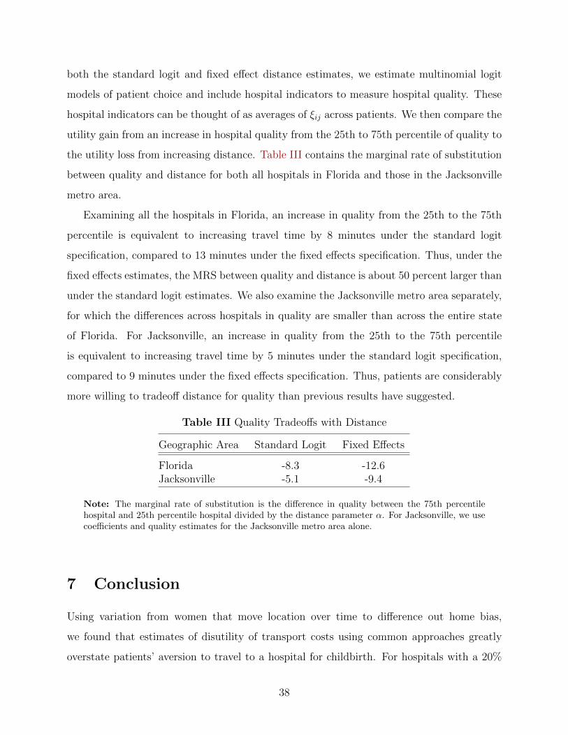
both the standard logit and fixed effect distance estimates, we estimate multinomial logit
models of patient choice and include hospital indicators to measure hospital quality. These
hospital indicators can be thought of as averages of ξij across patients. We then compare the
utility gain from an increase in hospital quality from the 25th to 75th percentile of quality to
the utility loss from increasing distance. Table III contains the marginal rate of substitution
between quality and distance for both all hospitals in Florida and those in the Jacksonville
metro area.
Examining all the hospitals in Florida, an increase in quality from the 25th to the 75th
percentile is equivalent to increasing travel time by 8 minutes under the standard logit
specification, compared to 13 minutes under the fixed effects specification. Thus, under the
fixed effects estimates, the MRS between quality and distance is about 50 percent larger than
under the standard logit estimates. We also examine the Jacksonville metro area separately,
for which the differences across hospitals in quality are smaller than across the entire state
of Florida. For Jacksonville, an increase in quality from the 25th to the 75th percentile
is equivalent to increasing travel time by 5 minutes under the standard logit specification,
compared to 9 minutes under the fixed effects specification. Thus, patients are considerably
more willing to tradeoff distance for quality than previous results have suggested.
Table III Quality Tradeoffs with Distance
Geographic Area Standard Logit Fixed Effects
Florida -8.3 -12.6Jacksonville -5.1 -9.4
Note: The marginal rate of substitution is the difference in quality between the 75th percentilehospital and 25th percentile hospital divided by the distance parameter α. For Jacksonville, we usecoefficients and quality estimates for the Jacksonville metro area alone.
7 Conclusion
Using variation from women that move location over time to difference out home bias,
we found that estimates of disutility of transport costs using common approaches greatly
overstate patients’ aversion to travel to a hospital for childbirth. For hospitals with a 20%
38

share, a one minute increase in travel time decreases demand by 9.7% under a standard logit
framework, compared to 5.4% under a fixed effect model that accounts for home bias. We
then showed that referral patterns could explain a substantial part of the difference between
the fixed effect and standard logit estimates.
We then examined three applications that demonstrate the importance of controlling
for home bias. In our first application, we showed that, when patients dislike travelling to
doctors more than travelling to hospitals, and doctors also dislike travelling to hospitals, we
can replicate our results on the impact of home bias on estimates of transportation costs.
In addition, a standard approach can greatly underestimate the extent to which two distant
hospitals are substitutes. In our second application, we examined a contested hospital move
in which concern was expressed that many patients living near the hospital’s old location
would not visit it at its new location. We show that our fixed effect estimates imply most of
these patients would travel to the new location, compared to standard models. In our third
application, we found that patients are more sensitive to quality, and so are more willing to
travel farther to visit a higher quality hospital, under the fixed effect estimates than under
a standard logit.
In this paper, we found evidence that referral patterns are a likely source of home bias,
and accounting for these patterns can change estimates of welfare effects from policy changes
such as mergers. Since this is true even when there is no change in referral patterns post-
merger, understanding referral patterns can be important to predict the welfare consequences
of policy changes. In addition, referral patterns themselves may change with a major change
in the economic environment, such as vertical mergers between physicians and hospitals, or
managed care, in ways that could substantially affect welfare. Thus, more research is needed
both in how physician incentives affect referral patterns, and how referral patterns affect
consumer welfare.
For future research, it would be useful to examine the generalizability of our results.
In this paper, we have only examined the choices of pregnant women. Transport costs
themselves may be more burdensome for pregnancy than other conditions, because pregnant
women need to get to the hospital quickly after labor begins, compared to more schedulable
procedures. In addition, referrals may be more salient in patient choice for some conditions
39

and less salient for others. Both of these channels would affect estimated distance coefficients
and the potential effect of not accounting for home bias.
40

References
Anas, Alex and Cheng Min Feng, “Invariance of expected utilities in logit models,” EconomicsLetters, 1988, 27, 41–45.
Anderson, James E, “The Gravity Model,” Annual Review of Economics, 2011, 3 (1), 133–160.
and Eric Van Wincoop, “Trade Costs,” Journal of Economic Literature, 2004, 42 (3), 691–751.
Backstrom, Lars, Eric Sun, and Cameron Marlow, “Find Me If You Can: Improving Geo-graphical Prediction with Social and Spatial Proximity,” in “Proceedings of the 19th InternationalConference on World Wide Web” ACM 2010, pp. 61–70.
Baker, Laurence, M. Kate Bundorf, and Daniel P. Kessler, “The Effect of Hospi-tal/Physician Integration on Hospital Choice,” Journal of Health Economics, 2016, 50, 1–8.
Balan, David and Keith Brand, “Simulating Hospital Merger Simulations,” FTC WorkingPaper No. 334, 2018.
Beckert, Walter and Kate Collyer, “Choice in the Presence of Experts: The Role of GeneralPractitioners in Patients’ Hospital Choice,” 2017.
Bergstrand, Jeffrey, “The Gravity Equation in International Trade: Some Microeconomic Foun-dations and Empirical Evidence,” The Review of Economics and Statistics, 1985, 67 (3), 474–481.
Berry, Steven T, “Estimating Discrete-Choice Models of Product Differentiation,” The RANDJournal of Economics, 1994, pp. 242–262.
Burns, Lawton R. and Douglas R. Wholey, “The Impact of Physician Characteristics inConditional Choice Models for Hospital Demand,” Journal of Health Economics, 1992, 11 (1),43–62.
Capps, Cory, David Dranove, and Mark Satterthwaite, “Competition and Market Powerin Option Demand Markets,” RAND Journal of Economics, 2003, 34 (4), 737–763.
, , and Richard C Lindrooth, “Hospital closure and economic efficiency,” Journal of HealthEconomics, 2010, 29 (1), 87–109.
Capps, Cory S, “From Rockford to Joplin and Back Again: The Impact of Economics on HospitalMerger Enforcement,” The Antitrust Bulletin, 2014, 59 (3), 443–478.
Chamberlain, Gary, “Analysis of Covariance with Qualitative Data,” The Review of EconomicStudies, 1980, 47 (1), 225–238.
Chandra, Amitabh, Amy Finkelstein, Adam Sacarny, and Chad Syverson, “HealthcareExceptionalism? Performance and Allocation in the US Healthcare Sector,” American EconomicReview, 2016, 106 (8), 2110–44.
Chaney, Thomas, “The Gravity Equation in International Trade: An Explanation,” Journal ofPolitical Economy, 2018, 126 (1).
41

Devers, Kelly J., Linda R. Brewster, and Lawrence P. Casalino, “Changes in HospitalCompetitive Strategy: A New Medical Arms Race?,” Health Services Research, 2003, 38 (1p2),447–469.
Doane, Michael J., Luke Froeb, and R. Lawrence Van Horn, “How Well Do Travel CostModels Measure Competition Among Hospitals?,” mimeo, 2012.
Farrell, Joseph, David J. Balan, Keith Brand, and Brett W. Wendling, “Economics atthe FTC: Hospital Mergers, Authorized Generic Drugs, and Consumer Credit Markets,” Reviewof Industrial Organization, 2011, 39 (4), 271–296.
Garmon, Christopher, “The Accuracy of Hospital Merger Screening Methods,” The RANDJournal of Economics, 2017, 48 (4), 1068–1102.
Gaynor, Martin and Kevin Pflum, “Getting Market Definition Right: Hospital Merger Casesand Beyond,” Antitrust Chronicle, 2017, 1, 31–39.
, Carol Propper, and Stephan Seiler, “Free to Choose? Reform, Choice, and Considera-tion Sets in the English National Health Service,” American Economic Review, 2016, 106 (11),3521,3557.
Glaeser, Edward L., Bruce I. Sacerdote, and Jose A. Scheinkman, “The Social Multiplier,”Journal of the European Economic Association, 2003, 1 (2-3), 345–353.
Goldenberg, Jacob and Moshe Levy, “Distance is Not Dead: Social Interaction and Geo-graphical Distance in the Internet Era,” arXiv preprint arXiv:0906.3202, 2009.
Gowrisankaran, Gautam, Aviv Nevo, and Robert Town, “Mergers when Prices are Ne-gotiated: Evidence from the Hospital Industry,” American Economic Review, 2015, 105 (1),172–203.
, Claudio Lucarelli, Philipp Schmidt-Dengler, and Robert Town, “Can AmputationSave the Hospital? The Impact of the Medicare Rural Flexibility Program on Demand andWelfare,” 2017.
Grogger, Jeffrey and Gordon H Hanson, “Income Maximization and the Selection and Sortingof International Migrants,” Journal of Development Economics, 2011, 95 (1), 42–57.
Hamilton, Brady E., Joyce A. Martin, Michelle J.K. Osterman, Sally C. Curtin, andT.J Mathews, “National Vital Statistics Reports,” National Vital Statistics Reports, 2015, 64(12).
Harris, Katherine M., “How do Patients Choose Physicians? Evidence from a National Surveyof Enrollees in Employment-Related Health Plans,” Health Services Research, 2003, 38 (2), 711–732.
Head, Keith and Thierry Mayer, “Gravity Equations: Workhorse, Toolkit, and Cookbook,”2013.
Helpman, Elhanan, Marc J Melitz, and Stephen R Yeaple, “Export Versus FDI withHeterogeneous Firms,” American Economic Review, 2004, 94 (1), 300–316.
42

Ho, Kate and Ariel Pakes, “Hospital Choices, Hospital Prices, and Financial Incentives toPhysicians,” American Economic Review, 2014, 104 (12), 3841–3884.
and , “Physician Payment Reform and Hospital Referrals,” The American Economic Review,2014, 104 (5), 200–205.
and Robin S Lee, “Insurer competition in health care markets,” Econometrica, 2017, 85 (2),379–417.
Ho, Katherine, “The Welfare Effects of Restricted Hospital Choice in the US Medical CareMarket,” Journal of Applied Econometrics, 2006, 21 (7), 1039–1079.
Hoerger, Thomas J. and Leslie Z. Howard, “Search Behavior and Choice of Physician in theMarket for Prenatal Care,” Medical Care, 1995, 33 (4), 332–349.
Holmes, Thomas, “The Diffusion of Wal-Mart and Economies of Density,” Econometrica, 2011,79 (1), 253–302.
Honore, Bo E and Ekaterini Kyriazidou, “Panel Data Discrete Choice Models with LaggedDependent Variables,” Econometrica, 2000, 68 (4), 839–874.
Hortacsu, Ali, F Martınez-Jerez, and Jason Douglas, “The Geography of Trade in OnlineTransactions: Evidence from eBay and Mercadolibre,” American Economic Journal: Microeco-nomics, 2009, 1 (1), 53–74.
Hotelling, Harold, “Stability in Competition,” The Economic Journal, 1929, 39 (153), 41–57.
Houde, Jean-Franois, “Spatial Differentiation and Vertical Mergers in Retail Markets for Gaso-line,” American Economic Review, 2012, 102 (5), 2147–2182.
Kane, Carol K., “Policy Research Perspectives - Updated Data on Physician Practice Arrange-ments: Physician Ownership Drops Below 50 Percent,” 2017.
Miller, Nathan, Marc Remer, Conor Ryan, and Gloria Sheu, “Upward Pricing Pressureas a Predictor of Merger Price Effects,” International Journal of Industrial Organization, 2017,52, 216–247.
Moraga-Gonzalez, Jose Luis, Zsolt Sandor, and Matthijs R Wildenbeest, “ConsumerSearch and Prices in the Automobile Market,” 2017.
Raval, Devesh and Ted Rosenbaum, “Decomposing the Welfare Impacts of Medicaid MCOSteering,” mimeo, 2016.
and , “Why Do Previous Choices Matter for Hospital Demand? Decomposing SwitchingCosts from Unobserved Preferences,” Review of Economics and Statistics, forthcoming.
, , and Nathan E. Wilson, “Using Disaster Induced Hospital Closures to Evaluate Modelsof Hospital Choice,” mimeo, 2017.
, , and Steven A. Tenn, “A Semiparametric Discrete Choice Model: An Application toHospital Mergers,” Economic Inquiry, 2017, 55, 1919–1944.
43

Romley, John A and Dana P Goldman, “How Costly is Hospital Quality? A Revealed-Preference Approach,” The Journal of Industrial Economics, 2011, 59 (4), 578–608.
Sacerdote, Bruce, “Peer Effects in Education: How Might They Work, How Big Are They AndHow Much Do We Know Thus Far?,” Handbook of the Economics of Education, 2011, 3, 249–277.
Saha, Somnath, Sara H. Taggart, Miriam Komaromy, and Andrew B. Bindman, “DoPatients Choose Physicians of Their Own Race?,” Health Affairs, 2000, 19 (4), 76–83.
Satterthwaite, Mark A., “Competition and Equilibrium as a Driving Force in the Health ServicesSector,” in “Managing the Service Economy Prospects and Problems,” Cambridge UniversityPress, Cambridge, 1985.
Schiller, Preston L. and Jeffrey S. Levin, “Is There a Religious Factor in Health Care Uti-lization?: A Review,” Social Science & Medicine, 1988, 27 (12), 1369–1379.
Shepard, Mark, “Hospital Network Competition and Adverse Selection: Evidence from the Mas-sachusetts Health Insurance Exchange,” 2016.
Tay, Abigail, “Assessing Competition in Hospital Care Markets: The Importance of Accountingfor Quality Differentiation,” RAND Journal of Economics, 2003, pp. 786–814.
Thomadsen, Raphael, “The Effect of Ownership Structure on Prices in Geographically Differ-entiated Industries,” RAND Journal of Economics, 2005, 36 (4), 908–929.
Wolf, Holger C, “Intranational Home Bias in Trade,” Review of Economics and Statistics, 2000,82 (4), 555–563.
44
For Online Publication
A Parametrization of Patient Heterogeneity
For our counterfactual experiments, we have to place further restrictions on patients’ unobserved
preferences for hospitals. We assume that ξij only varies with the zip code where women live at the
time of their first birth. Therefore, we can rewrite ξij = µzj , where µzj is the mean within woman
i’s zip code z at the time of their first birth.
Using this assumption, we recover µzj by focusing on the full population of first time mothers.
Rewriting equation (3) for this population of women, we obtain:
uij1 = −αdij1 + µzj + εij1.
Since we only observe distance at the zip code level, we can write this as:
uij1 = −αdzj1 + µzj︸ ︷︷ ︸µzj
+εij1.
Since εij1 is distributed type I extreme value, we obtain:
Prij1 =exp(µzj)∑j exp(µzj)
.
Using the transformation discussed in Berry (1994), we can recover:
µzj = log(szj1)− log(s0z1),
where szj is the share of first time mothers in zip code z giving birth in hospital j, and s0z1 is the
share of women giving birth outside of their service area.
B Social Multiplier Model
In this section, we develop a model in which a patient’s utility for a hospital depends both upon
distance and the average of her friends’ utilities, similar to models used in the social multiplier
literature (Glaeser et al., 2003).
Deterministic utility δij for individual i and hospital j is:
δij = αdij +γ
N − 1
∑f∈Fi
δfj ,
where Fi is the set of i’s friends and N − 1 is the number of friends. The parameter γ determines
how important average friend utility is for individual i’s utility. For simplicity, we assume that
45

everyone is friends with everyone else. In that case, we can solve for δij as a function of individual
i’s own distance and the average friend distance:
δij = αdij + αγ
1− γ1
N − 1
∑f∈Fi
dfj .
First take the case in which all of the friends live in the same location, so, ∀f ∈ Fi, dij = dfj .
In that case, we have that:
δij = α1
1− γdij .
Here, 11−γ is the social multiplier of the effect of distance; it collapses to 1 when γ is zero, and
is 2 when γ is 0.5.
Now take the case in which friends do not live at the same location. In that case, we have that
the ratio in individual i’s probability of visiting hospitals j and l is:
PrijPril
=exp(δij)
exp(δil)= exp(α(dij − dil) + α
γ
1− γ(
1
N − 1
∑f∈Fi
(dfj − dfl)).
Thus, the relative probability of going to hospital j over hospital l depends both upon the
difference in i’s distance, and the average difference in all of the friends’ distance. We can always
partition the average difference in all of the friends’ distance into a component correlated with i’s
distance and a part uncorrelated with i’s distance:
1
N − 1
∑f∈Fi
(dfj − dfl) = βjl(dij − dil) + ε,
where the coefficient βjl is the regression coefficient of the average friends’ difference in distance
on individual i’s difference in distance:
Cov(dij − dil, 1N−1
∑f∈Fi
(dfj − dfl))V ar(dij − dil)
,
and ε is uncorrelated with dij−dil by definition. In that case, we can rewrite the relative probability
of going to hospital j over hospital l as
PrijPril
= exp(α(1 + βjlγ
1− γ)(dij − dil) + ε),
which collapses to the formula in which all friends live in the same location, so βjl is one and ε
always zero. Thus, when friends do not all live in the same location, how close each of the friends
lives will affect the social multiplier – the closer they live, so their distances to providers are more
highly correlated, the higher the social multiplier.
46

C Ex-Ante Utility and WTP
In the logit model, the expected decline in patient i’s welfare from excluding a set of hospitals
S ⊂ J is as follows:
WTPiS = − ln(1−∑j∈S
sij). (7)
A patient’s WTP is an increasing function of the probability she will select a hospital in set S,
and equals zero when that probability is zero. Overall WTP is obtained by adding up patient-level
WTP across all patients.
The antitrust agencies have used WTP to assess the expected harm from a merger of two
hospital systems (Farrell et al. (2011)). The combined system’s bargaining position changes post-
merger, since it can now threaten to exclude both systems simultaneously from the provider’s
network. Let WTP12 represent the WTP for the combined system, and WTP1 and WTP2 for
System 1 and System 2 individually. If the two systems are substitutes, then the loss in welfare from
simultaneously excluding both systems exceeds the sum of the losses from individually excluding
each system. The percentage increase in WTP resulting from a merger between the two systems
can then be calculated as follows:
∆WTP12 =WTP12
WTP1 +WTP2− 1. (8)
This measure has the property that it equals zero when the two systems are not substitutes, and
is an increasing function of the level of substitution between the two systems.
D Additional Graphs and Tables
47

Figure 12 Robustness Checks for Estimates of the Transport Cost Coefficient Using theStandard Logit Model
Note: The red lines are the elasticity estimates from the standard logit model while the blue linesare the elasticity estimates from the fixed effects model. The solid lines are the point estimateswhile the dashed lines are the 95% confidence interval. The black horizontal lines are the elasticityestimates from our robustness checks conducted under the standard logit specification. The dot isthe point estimate and the lines are the 95% confidence interval. Logit estimates reflect the transportcost parameter α; the semi-elasticity with respect to transport costs is α multiplied by one minusthe probability of going to the hospital. See Table VI for a table of the estimates and standarderrors used to generate this figure.
48

Table IV Parameter Estimates: Main Results
Standard Logit (Age Restriction) Standard Logit (Chamberlain) Fixed Effect
Time -0.121 -0.116 -0.068(0.000) (0.001) (0.002)
Hospital/PatientFixed Effects
X
N 626,738 38,591 16,718
Note: All specifications include time invariant hospital indicator variables. N givesthe units of observation used to compute the asymptotics. For the models that includehospital/patient fixed effects, this is the number of women, while for the other discretechoice models this is the number of admissions. The age restriction sample includes allwomen in Florida that were of age 21 or less in 2006. The Chamberlain sample onlyincludes women in the age restriction sample who move houses and switch hospitalsbetween their first and second birth.
49

Table V Parameter Estimates: Main Results Robustness
Point Estimate(Std. Error) N
Normal Delivery -0.068 11,031(0.002)
Normal Vaginal -0.070 7,797(0.002)
Normal C Section -0.063 2,409(0.004)
Term Delivery -0.068 15,433(0.002)
Age Cutoff at 18 -0.071 8,996(0.002)
Same Income Move -0.065 8,835(0.002)
Jacksonville MSA -0.072 2,168(0.005)
Same Clinician -0.042 937(0.007)
Commercial Insurance -0.054 1,340(0.005)
Large Moves -0.069 1,136(0.004)
Small Moves -0.064 12,878(0.002)
Note: All specifications include time invariant hospital/patient fixed effects. N givesthe units of observation used to compute the asymptotics - the number of women. Thesamples for each regression are restricted as follows. “Normal Delivery” only includespatients with a normal labor and delivery for both births, while “Normal Vaginal”and “Normal C-Section” further restricts to patients with two normal vaginal or C-Section deliveries respectively, and “Term Delivery” restricts to patients with a termdelivery. “Same Clinician” only includes patients with the same operating physician forboth births. “Large Moves” and “Small Moves” only include women whose distance toboth hospitals changes by more than 15 minutes, or less than 15 minutes, respectively.“Age Cutoff at 18” only includes women who were at most 18 in 2006. “Same IncomeMove” only includes women for whom the zip code median household income changesby less than $10,000 between births. “Commercial Insurance” only includes womenusing commercial insurance for both births. Finally, “Jacksonville MSA” only includeswomen residing in the Jacksonville MSA for both births.
50

Table VI Parameter Estimates: Standard Logit Results Robustness
Point Estimate(Std. Error) N
Age Cutoff at 18 -0.124 359,416(0.000)
Commercial Insurance -0.111 142,141(0.000)
Jacksonville MSA -0.120 56,726(0.001)
Medicaid -0.125 452,974(0.000)
Normal Vaginal -0.123 363,681(0.000)
Normal C Section -0.120 135,651(0.000)
Note: All specifications include hospital indicator variables, but do not include timeinvariant hospital/patient fixed effects. N gives the units of observation used to computethe asymptotics - the number of admissions. The samples for each regression arerestricted as follows.“Normal Vaginal” and “Normal C-Section” further restricts topatients with normal vaginal or C-Section deliveries respectively. “Age Cutoff at 18”only includes women who were at most 18 in 2006. “Commercial Insurance” onlyincludes women using commercial insurance, while “Medicaid” only includes women onMedicaid insurance. Finally, “Jacksonville MSA” only includes women residing in theJacksonville MSA.
51

Table VII Parameter Estimates: Referral Mechanism
Clinician Month Clinician Week Clinician First Birth
Time -0.093 -0.095 -0.097(0.001) (0.000) (0.001)
Clinician/Hosp Use 7.793 5.352 1.362(0.020) (0.010) (0.008)
N 626,738 626,738 147,661
Note: All specifications include hospital indicator variables, but do not include timeinvariant hospital/patient fixed effects. N gives the units of observation used to computethe asymptotics - the number of admissions. The second column includes an indicatorfor every hospital for which the obstetrician delivers an average of more than one babyper month, the third column includes an indicator for every hospital for which theobstetrician delivers an average of more than one baby per week, and the fourth columnonly includes second births and includes an indicator for every hospital for which theobstetrician at first birth delivers an average of more than one baby per month.
Table VIII Parameter Estimates: Switching Cost Mechanism
Switching Cost First Birth
Time -0.117 -0.121(0.000) (0.000)
N 626,738 432,390
Note: All specifications include hospital indicator variables, but do not include timeinvariant hospital/patient fixed effects. N gives the units of observation used to computethe asymptotics - the number of admissions. The second column includes an indicatorfor the hospital previously chosen by the patient calibrated using the switching costparameter estimated in Raval and Rosenbaum (forthcoming), while the third columnonly examines first births.
52

Table IX Parameter Estimates: Catering To Local Demand Mechanism
Catholic Spanish Birth Room
Time -0.121 -0.121 -0.121(0.000) (0.000) (0.000)
Cath School X Cath Hosp 0.002(0.011)
Hispanic Pat X Spanish Hosp 0.122(0.020)
Median Income X Birth Rm 0.790(0.284)
N 626,738 626,738 622,212
Note: All specifications include hospital indicator variables, but do not include timeinvariant hospital/patient fixed effects. N gives the units of observation used to computethe asymptotics - the number of admissions. The second column interacts whether thehospital is affiliated with the Catholic Church with whether the patient’s zip code hasa Catholic school, the third column interacts whether the patient is Hispanic with thefraction of obstetricians with admitting privileges at the hospital that speak Spanish,and the fourth column interacts zip code median income with whether the hospital hasa birthing room.
53