WHY DON’T PEOPLE VOTE?: A QUANTITATIVE STUDY AND ANALYSIS OF VOTER

TURNOUT IN MAYORAL ELECTIONS IN LARGE AMERICAN CITIES

Michael Patison

TC660H

Plan II Honors Program

University of Texas at Austin

Supervisor: Dr. Zachary Elkins, Department of Government

Second Reader: Dr. Daron Shaw, Department of Government

Abstract

Author: Michael Patison

Title: Why Don’t People Vote?: A Quantitative Study and Analysis of Voter Turnout in Mayoral

Elections in Large American Cities

Supervising Professors: Dr. Zachary Elkins, Department of Government, and Dr. Daron Shaw,

Department of Government

Voter turnout is one of the most important keys to a fully functioning representative

democracy. Without an actively voting electorate, the American democratic experiment ceases to

function properly. As such, voter turnout is of paramount importance in understanding the health

of American democracy and the institutional and demographic hurdles that stand in its way.

Most research on voter turnout as a general concept in American democracy is focused on the

national and state levels, but municipal governments arguably have a greater impact on the day-

to-day lives of the citizenry. Four questions were examined by the study. These questions

revolved around why turnout in mayoral elections is so low, what factors are most important is

helping dictate how high municipal voter turnout is, and how these factors may help explain

differences in turnout between cities with different levels of turnout. The analysis found that, at

least in the largest American cities, turnout in mayoral elections is largely contingent on when

elections are held, how important the highest office on the ballot is, and how competitive the

electoral contest is.

Acknowledgements

Much credit for my success with the thesis goes to my parents, John and Michelle, for

their unending support.

I would also like to thank my advisor and second reader, Drs. Zachary Elkins and Daron

Shaw, for their advice and recommendations.

Finally, I would like to thank Plan II for giving me a second chance to try to get it right

the second time around.

Table of Contents

Chapter 1: Introduction ....................................................................................................................1

Chapter 2: Literature Review ...........................................................................................................8

Chapter 3: Data Methodology, Presentation, and Analysis ...........................................................21

Chapter 4: Discussion, Conclusions, and Recommendations ........................................................43

Appendices .....................................................................................................................................47

Works Cited ...................................................................................................................................59

Patison 1

Chapter 1: Introduction

Voter turnout is one of the most important keys to a fully functioning representative

democracy. Without an actively voting electorate, the American democratic experiment ceases to

function properly. As such, voter turnout is of paramount importance in understanding the health

of American democracy and the systemic and demographics hurdles that stand in its way. Robust

voter turnout is not only an important component of a healthy U.S. democracy, but also in a

representative democracy that represents all the nation’s citizens. After all, it was Founding

Father John Adams who said that a “representative assembly…should be, in miniature, an exact

portrait of the people at large” (Adams, 1776). As such, much attention has been paid to voter

turnout, both in terms of what drives it and in terms of what its effects are.

Most research on voter turnout as a general concept in American democracy is focused

on the national and state levels, be it in Presidential elections or congressional ones (find two or

three examples to cite). While certainly most valued, at least in public reckoning, offices on the

national stage often have less bearing on peoples’ day-to-day lives than do municipal officials,

namely those on city councils, local boards, and county commissions.

Municipal governments truly are the unsung heroes of American government and

administration. City councils and mayors make sure residents have clean water and sewage

services and decide where to put parks and how to manage their upkeep. City governments

decide how often garbage is collected and make sure it gets picked up. They also make decisions

regarding public transportation, zoning, and law enforcement, not to mention acting as city-brand

ambassadors to potential business investment in the area in the form of new offices and new

jobs.

Patison 2

While less attractive politically and interest-wise than flashy national bodies, municipal

governments arguably have a greater impact on the day-to-day lives of the citizenry.

Nevertheless, in a country known for relatively low voter turnout in even the most high-profile of

electoral contests, voter turnout in municipal elections is particularly abysmal. As such, more

contemporary research is needed to fully understand the issues at play in municipal electoral

politics.

This contemporaneous aspect is key. Starting in the mid-1960s, political scientists

worked tirelessly on urban politics in generally, and urban voting more specifically (Alford &

Lee, 1968). These works were intersectional in focus, spending the majority of their time

examining the systems and institutions that depress voter turnout. This trend continued through

the early 1990s (Bullock, 1990), with Who Votes? occupying a landmark position in the dialogue

(Wolfinger & Rosenstone, 1980). These other works furthered the conversation, discussing not

just the systems and institutions, but the political and social cultures and stakes involved. In other

words, voter turnout has been studied in terms of how it was driven rather than which people

actually vote and what that population segment voting leads to.

Research Problem Statement

The dialogue since roughly 2000 has focused much more on examining both the effects

of low voter turnout and how specific aspects of demographics or institutionalism impact voter

turnout. These blindered approaches are overly cautious and conservative and fail to account for

important inter-variable connections and applications that could help better explain voter turnout

in cities. In addition, it has left a dearth of more modern information and findings about cities

people live in today. This has left the academic community reliant upon outdated information

and analysis gathered from cities sometimes as much as half a century ago.

Patison 3

This thesis will provide an update to the intersectional dialogue established decades ago

by examining voter turnout in a more syncretic context. Instead of asking how race or

demographics in general affect turnout, this thesis will discern whether race and/or demographics

are important urban voter turnout indicators in the first place, before determining what effect

they might have on eventual turnout. This is important because, for many, deciding whether or

not to vote involves a cost-benefit analysis. In a pool of thousands of votes, how much does a

single vote really matter, and, as such, how much benefit does it really bestow upon the voter.

The largest benefit to a voter is arguably the sense of satisfaction one has after voting, but even

this may be outweighed by high costs and barriers to entry involved in voting in some contests.

This thesis will also examine institutional factors of municipal government in an attempt to

discern the impact they have on voter turnout at the local level. Only if these institutional and

demographic factors are indeed important indicators is their study in a voter turnout context

wholly worthwhile.

Research Questions

This thesis will examine and answer four interrelated research questions in order to

provide a thorough exploration of mayoral election voter turnout.

Firstly, why is voter turnout in mayoral elections in so low? Voter turnout in the United

States is already low, rarely, if ever, surpassing 60% in national elections. This is one of the

lowest voter turnout rates of any fully functioning democracy in the world. But despite how low

turnout is, voter turnout in mayoral and other municipal elections plumbs new depths, with many

cities hovering around 30% participation, and multiple falling below 10% (Morlan, 1984).

Patison 4

Secondly, which are the most important variables for predicting a municipal election’s

voter turnout? As previously stated, there seems to be a proclivity to chalk low voter turnout up

to race or some other demographic factor. But is this really a rational viewpoint?

Thirdly, why is voter turnout lower in some cities than in others? Despite some cities’

abysmal turnout figures, other cities manage to soar about the rest.

Finally, what factors may or may not account for these disparities in voter turnout

between cities? Are they the same factors that help predict turnout more generally? Are policy

and campaign issues more potent in some cities than in others. Do some cities just have a more

vibrant culture of political engagement and voting?

Research Method and Presentation

I took a two-pronged approach to answering these questions. First, I conducted a

literature review. Second, I utilized a data set of my own compilation to assess voter turnout in

the nation’s 107 largest cities, which accounts for all American cities with populations over

200,000, as of the 2010 U.S. Census. Both of these aspects are discussed in more detail below.

Literature Review Process

The literature review will examine the history of the available literature and discourse on

voter turnout and urban voting, synthesizing them through comparison and contrast of research

with similar focuses.

The review will begin with an examination of the existing literature on both voter turnout

theory and voter choice theory. Throughout the 1960s and 1970s, urban voting was an important

topic in political academics. Since then, however, the discourse has been replaced by largely

reductionist examinations that either focus exclusively on national elections or that examine

urban politics solely as an issue of race rather than any sort of complex, intersectional issue that

Patison 5

certainly includes race, but is not limited to it. The literature review will identify common

thematic elements and arguments between works to paint a more complete picture of the existing

literature, rather than a segmented one. It will do so by tracing the discourse on five groups of

variables

The first section will be a discussion of the impact of low voter turnout on representation

and other factors, predominantly in a local context. The following sources will be included:

Alford and Lee (1968), Wolfinger and Rosenstone (1980), Morlan (1984), Bullock (1990),

Hajnal and Lewis (2003), Hajnal and Trounstine (2005), Hajnal (2010), and Oliver, Ha, and

Callen (2012).

The second section will focus on political structure and will be subdivided in four

separate sections: statutory nonpartisanship, form of government, election format, and election

scheduling. The larger section with be introduced using Wolfinger and Rosenstone (1980).

Statutory nonpartisanship will focus on whether municipal elections are held on a

nonpartisan basis or a partisan one. This section will utilize work from Kessel (1962), Schnore

and Alford (1963), Alford and Scoble (1965), Alford and Lee (1968), and Hajnal and Lewis

(2003).

Form of government will deal with whether a city has a mayor-council or a council-

manager form of government. This political versus administrative divide will be contributed to

by Kessel (1962), Schnore and Alford (1963), Alford and Scoble (1965), Alford and Lee (1968),

Wood (2002), and Hajnal and Lewis (2003).

Election format will center on how people are elected, namely whether first-past-the-post,

ranked-choice voting, or some form of limited voting is used. Mcdaniel (2016) will form the

entirety of this shorter discussion.

Patison 6

Election scheduling will be focused on Hajnal’s works with Lewis and Louch (2002,

2003), with some input from Wood (2002). Election timing is when the elections is held, such as

in May of an off-year, or in November of a Presidential election year.

The third section will cover demographics and socioeconomics, focusing on voter turnout

with respect to race and economic circumstances. This section will utilize the following sources:

Alford and Lee (1968), Wolfinger and Rostenstone (1980), Wood (2002), Hajnal and Trounstine

(2005), and Oliver, Ha, and Callen (2012).

A short section will look at the work done on political participation in urban areas. This

section will look at work done by Oliver (2000), Kelleher and Lowery (2008), and Carr and

Tavares (2012).

The final section will look at the impact of a city’s intangible political culture on voter

turnout in local elections. Alford and Lee (1968), Wolfinger and Rosenstone (1980), Verba,

Schlozman, and Brady (1995), Oliver (2000), Hajnal, Lewis, and Louch (2002), Kaufmann

(2004), Oliver, Ha, and Callen (2012), and Rolfe (2012) will form the basis of this section.

Quantitative Analysis of City Demographics and Voter Turnout

The quantitative analysis will utilize institutional, demographic and voter turnout data

from each of the three most recent mayoral elections in each of the nation’s 107 largest cities by

population, according to the 2010 U.S. Census. These 107 cities constitute every American city

with a population over 200,000, as of 2010. A list of these cities, along with their population as

of 2010, are included in Appendix A. These elections total 321 separate independent data points.

Citizens of voting age population (CVAP) and other data ranging from race and election timing

to educational achievement and household income levels and from population density to voter

registration laws complete the data set. Multiple regression statistical analysis techniques will

Patison 7

then be applied to determine variable correlation to voter turnout, thereby revealing the most

potent factors in determining physical civic engagement in electoral politics. The statistical data

compiled falls into two main categories: institutions and demographics.

The election data is composed of the following 14 data points: election scheduling by

month; whether the incumbent ran; the length of the term up for election; whether the city has a

strong mayor with a city council or a strong city council with a city manager; whether there is

same-day voter registration; how many potential elections it could take to elect the mayor; which

election stage was decisive; whether the elections are officially partisan or nonpartisan; whether

first-past-the-post or ranked-choice voting is used; the voter turnout (CVAP/raw turnout

excluding invalid votes); the number of candidates in the decisive round of voting; what the

highest elected office on the ballot was; and a competition index. The competition index is

expressed mathematically as follows:

(Margin of Victory/Square Root (Number of Candidates))

________________________________

Raw Turnout

The demographic data entails the following nine variables: racial demographics, limited

to white, African American, Hispanic, Asian, and Others; median household income; high school

graduation rate; bachelor’s degree rate; the rate of married people with children under 18;

percentage over 65; which Census Bureau region the city is located in; and the population

density.

Patison 8

Chapter 2: Literature Review

Psephology, the study of elections, has seen a fruitful discourse in the United States since

its origins in the early 1960s. From Alford and his associates and Wolfinger and Rosenstone, to

the more current works of Hajnal and Oliver, elections have seen a constantly evolving set of

important variables and varying degrees of interest in others. First, this literature review will look

at voter turnout as it pertains to the impact municipal government has on citizens’ everyday life

in big cities, as well as how turnout affects election results and representation of minorities and

members of lower socioeconomic groups in government. This literature review then will

undertake a methodical, variable-by-variable scrutiny of voting at the municipal level in

America. The variables examined will be: political structure, demographics, and city size.

Political structure will be divided into five subheadings: voter registration, statutory

nonpartisanship, form of government, election format, and election scheduling.

Impact of Low Voter Turnout

High level issues and the decisions made about them at the highest levels of government

rarely interact with residents’ lives on a consistent daily basis. On the other hand, municipal

government decisions impact residents’ lives more keenly on a daily basis. While there are

discrepancies between the services that larger and smaller municipalities directly provide for

their citizens, the majority of large cities in American provide street repair, parks, water, and

sewage for their citizens, in addition to police and fire departments (Oliver, Ha & Callen, 2012).

These important services alone should indicate the impactful day-to-day operation of cities and

their local government infrastructures.

Yet the voter turnout for these important local contests is exceedingly low. Turnout in

city elections average roughly half of the 50-55% seen in national elections. This, along with an

Patison 9

observable downward trend in these already low turnout levels, points to a growing problem in

our democratic system’s most basic units (Alford & Lee, 1968; Morlan, 1984; Hajnal & Lewis,

2003).

The impact of low turnout has been an issue of record for quite some time. Until recently,

however, this focus has been on its impact on national elections. Surveys of voters and non-

voters, for instance, have found that both groups tend to have similar preferences (Wolfinger and

Rosenstone, 1980). Additionally, further attempts to establish whether either major political

party would benefit more from elevated turnout have been either inconsistent with other findings

or insignificant or both. (Hajnal, 2010).

There has been some evidence, more anecdotal than longitudinal, that minority

candidates tend to encourage minority participation (Bullock, 1990), but this seems outweighed

by evidence that the opposite is true. This oppositional evidence shows that, if minorities were to

vote in higher numbers in cities with larger minority populations, there is a high likelihood that

they could sway the outcome of the election in about one-third of the cases, and have a

significant impact on the victory margin in most other instances. Despite this finding, however,

African Americans largely lack the voting power necessary in America’s largest cities to have

the outsized impact necessary to sway elections in the same way that Hispanic constituencies do.

Nevertheless, There is little evidence that minorities do vote more in local elections when

someone who looks like them is running (Hajnal & Trounstine, 2005).

Some argue, however, that “low turnout is not a problem [for the overwhelming number

of American municipalities] because of the types of people who vote in local contests” (Oliver,

Ha & Callen, 2012). The argument here, however, seems to be a based on assumptions about the

representativeness of long-term residents and other politically active groups. It also seems to

Patison 10

vastly underestimate, or otherwise ignore, the importance of ethnic and racial representativeness

not just at higher levels, but at the local level as well. The fact of the matter is that “those who do

turn out to vote look very different from those who do not,” which results in a skewed vote that

often fails to take into account the concerns of all interest groups (Hajnal & Trounstine, 2005).

Political Structures

Arguably the largest amount of literature to do with voter turnout at the local level at least

partially focuses on the effect that various political structures have on turnout. The conversations

involved in the considerations of these topics are important, including more concrete issues like

voter registration, mayoral power, statutory nonpartisanship, and more amorphous things like

political vibrancy and innate political interest, knowledge, and engagement.

Voter Registration

Voter registration is a logical place to start examining these political structures and

strictures as it is the first step necessary to be able to vote in any governmental election. The

most commonly repeated theories are 1) that turnout will be higher where there are fewer

obstacles to voting, and 2) those with the least education, who are often also the poorest, with

have the most trouble navigating the bureaucratic elements of voter registration. Due to the

relatively recent passage of the Voting Rights Act and its subsequent Amendments in 1965 and

1970, respectively, Wolfinger and Rosenstone devote quite a bit of time to voter registration

requirements and laws and the impact they have on turnout. They found that the most powerfully

depressive laws were registration closing dates. Without these closing dates, they estimated there

would have been a turnout 6.1% higher in the 1972 national elections (Wolfinger & Rosenstone,

1980). While this is based on old data and national elections, it still stands to reason that same-

Patison 11

day voter registration, which the study seems to be advocating for in practice though not in

name, would still be likely to encourage higher turnouts.

Statutory Nonpartisanship

The differences in turnout between partisan and nonpartisan local elections has also had

focus on it since arguably the beginnings of local voter turnout examinations. Cities began

adopting nonpartisan municipal offices in the late 1890s and early 1900s, and as late as the

1910s, as part of the larger Progressive Reform Movement. These reforms were aimed at

reducing, and hopefully eliminating, the corruption and anti-democratic practices often seen in

some of America’s biggest cities, particularly those run by political machines. Making municipal

elections nonpartisan was one aspect of these reforms. The goal was to eliminate the ability to

vote purely based on partisanship, eliminating corrupt officials’ abilities to dictate voters’

choices completely along on party lines. While this reform proved an effective anti-corruption

tool, it also has hurt turnout as the often white, Anglo-Saxon Protestant groups that predominated

the Progressive voting blocs no longer predominate quite so much. For many less-educated

voters and many educated voters who are not particularly interested in municipal politics, the

nonpartisanship of elections often proves to be a barrier to entry. As such, nonpartisanship tends

to reduce voter participation. The participation gap created between partisan and nonpartisan

elections can vary greatly, but nevertheless exists, and has been measured to be as high as 20%

(Kessel, 1962; Schnore & Alford, 1963; Alford & Scoble, 1965; Alford & Lee, 1968). This

depression of turnout brought on by nonpartisanship has been a consistent finding (Hajnal &

Lewis, 2003).

Patison 12

Form of Government

In addition to statutory nonpartisanship, the Progressive Reform Movement chose

municipal government forms as a primary target for change. Until that point, cities usually had

been run by a mayor, supported by a city council, which will heretofore be called the mayor-

council form. Reformists, for essentially the same reasons as statutory nonpartisanship, called for

a more technocratic approach, in which the mayor may be directly and separately elected, but is

otherwise the first-among-equals. In this form, heretofore called council-manager, the mayor has

the power of a normal councilmember, but little more, and an unelected city manager handles the

day-to-day operation of the city. Like statutory nonpartisanship, these reforms were most

predominantly undertaken in “‘white, Anglo-Saxon, Protestant, growing, and mobile cities’”

(Kessel, 1962; Schnore & Alford, 1963; Alfred & Scoble, 1965; Alford & Lee, 1968). This

outsourcing of decision-making to unelected officials has often been cited as an important

contributor to lower turnout (Alford & Lee, 1968; Wood, 2002; Hajnal & Lewis, 2003).

In a mayor-council system, the mayor has more influence over policy and administration,

so they get all the credit and all the blame for the city’s successes and/or failures. Constituents,

therefore, have a much better understanding both of the mayor’s importance, and of their

opinions of the mayor’s abilities. In a council-manager system, the mayor acts almost as a

figurehead. The mayor may have policies in mind but often needs city council approval to make

the policy actionable, and the unelected, hired city manager is the person who actually makes the

administrative decisions that enact the policy. As such, the mayor in a council-manager system is

has roughly two degrees of separation between their choices and actual action, greatly reducing

the position’s power. Studies of size have found statistically significant correlation between form

of government and voter turnout (Wood, 2002).

Patison 13

There are other important administrative aspects that differentiate how turnout might look

on a city-to-city basis, too, including how many basic services, like water, electricity, or garbage

collection. This aspect of city service outsourcing seems quite a potent one. If the municipal

government does not provide electricity or water or garbage collection or a fire department, there

is reason to presume that the government is not as near to the forefront of the everyday person’s

mind. As such, it also stands to reason that this lower government visibility would harm both

public interest and public knowledge of their elected municipal officials, lowering turnout

(Hajnal & Lewis, 2003).

Election Format

The United States has always either used the first-past-the-post system or the two-round

runoff system. There has been some expression of hope in psephology circles that alternative,

more proportional electoral methods, such as ranked-choice voting (RCV), would yield higher

voter turnout. A study of San Francisco’s mayoral and city council elections, however, has found

that this is not the case. It seems that the information costs are too constraining for many casual

and/or less educated voters. RCV tends to necessitate a more complicated ballot structure, which,

combined with San Francisco’s decision to limit preferences to three, has corresponded to a

higher overvote percentage more on-par with hanging chads on punch-cards. These more

complicated ballots tend to overwhelmingly harm the African American and Hispanic

communities, as well as foreign-born voters, particularly those with language difficulties. Not

only has turnout in San Francisco remained stagnant, the percentage of voters utilizing the

ranking mechanism to its fullest extent has experienced a roller-coaster-like fluctuation, first

dropping by more than half, before more than doubling just one election later. RCV also tends to

obscure the benefits potentially reaped by minority groups, or at the very least how minority

Patison 14

voting behavior influences elections, by making it more difficult to accurately judge minority

voter first preferences, and decreasing racial group competition, which has the potential to lower

turnout. This decrease in racial group competition has had the effect of lowering minority

turnout, particularly among African Americans, who experienced a turnout decrease of over

20%. That said, a viable, competitive candidate within a voter’s racial or ethnic group did

noticeably increase turnout among all groups other than Hispanics (Mcdaniel, 2016).

Election Scheduling

Yet another by-product of the Progressive Reform Movement was the decision to make

municipal elections non-concurrent with national elections. This decision was ostensibly made to

wrest power from political parties and corrupt bosses of political machines, who, it was felt, used

the concurrent elections to their own benefit. For instance, it is much easier to sway an election

by illegal means, such as vote-buying or double-voting, when every election is happening at the

same time (Goodnow, 1908). Whether this reform had the desired effect is debatable, but there is

considerable evidence that non-concurrent elections have had deleterious effects on voter turnout

in local elections. This non-concurrence with elections for higher office seems to make local

elections extraordinarily costly, with little reward, for the average resident on multiple levels

(Hajnal & Lewis, 2003). First, learning about municipal election candidates is not always easy.

Second, many urban residents do not have the financial ability to leave their jobs in order to vote,

and an election with significantly lower stakes is rarely a good enough reason to lose an hour’s

wages or more. Third, while turnout in local contests is low, the time cost-benefit analysis of

spending the time waiting in line to vote for municipal offices rarely resolves in favor of the

potential benefits.

Patison 15

On the other hand, it seems almost obvious that turnout in local elections would increase

if they were held simultaneously with national elections. All voters would need to do is take a

few extra minutes to complete voting for the local offices, greatly reducing the costs associated

with voting in local elections. Not only would it aid in the reduction of voters’ decision costs, it

would also lower monetary costs for cities, which, along with the counties in which they are

located, tend to be in charge of paying for all elections and runoffs held non-concurrently with

national elections (Hajnal & Lewis, 2003).

There is evidence to suggest that holding concurrent local, state, and national elections

has an impact three times the size on voter turnout than does form of government, with total

concurrency yielding turnout nearly 30% higher than average (Wood, 2002). Peak-cycle

elections, which are classified as presidential primaries and general elections, as well as

congressional midterms, negate the importance of local institutions. Similarly, when focusing on

election timing, the importance of mayoral power is also insignificant. These findings stick to the

overall idea of the vast majority of research that “institutional features that tend to increase the

stakes of city elections also tend to increase turnout” (Hajnal & Lewis, 2003). This increasing of

stakes, however, does not seem to translate or transfer to non-institutional features, like general

senses regarding the competitiveness of a given local election. Even “high-stakes” contests that

seem competitive and might be expected to have higher levels of participation rarely do (Hajnal,

Lewis, & Louch, 2002). As such, it stands to reason that these institutional factors, specifically

election timing, are more significant players in driving voter turnout in local contests than more

abstract things like political culture and environmental and electoral competitiveness.

Patison 16

Demographics and Socioeconomics

Focus on the demographic and socioeconomic factors is a longstanding avenue of inquiry

into voter turnout and who votes. On a national election level, there have long been a few

generally accepted facts. Citizens of higher socioeconomic status vote more. This is true

regarding education level, income, or occupation. College graduates vote more than high school

graduates, and white-collar workers vote more than blue-collar workers. Additionally, the rich

generally vote more than the poor. When separated into individual, disaggregated variables,

education has the highest and most predictable influence on voter turnout in national elections,

with college graduates 38% more likely to vote than those with low levels of schooling. On the

other hand, income has a smaller effect on voter turnout. Beyond incomes providing

comfortability, income does not matter. The only identifiable difference in turnout is between

those with the lowest incomes and the middle class. Even this 14% difference pales in

comparison to the turnout differential found in education levels. The richest groups are no more

likely to vote than the middle classes. Finally, the white collar-blue collar dichotomy is not

significant. Instead, occupational responsibilities and job and time requirements are more

significant in determining turnout. This lack of linearity makes occupational impact on voter

turnout difficult to predict at the national level (Wolfinger & Rosenstone, 1980).

At the local, rather than the national, level, these socioeconomic factors are not as

pronounced. Some studies have found that cities with higher ethnic diversity and lower levels of

educational attainment actually have higher turnout (Alford & Lee, 1968). Other studies have

found the opposite, including a negative relationship between black population percentage and

voter turnout. There is also evidence that, contrary to Wolfinger and Rosenstone’s findings, at

the local level, income level, level of educational attainment, and African American population

Patison 17

percentage are statistically insignificant (Wood, 2002; Hajnal & Trounstine, 2005; Oliver, Ha, &

Callen, 2012). Despite this last finding, there is still evidence that, at the local level, whites vote

at much higher levels than Hispanics, Asians, and African Americans (Hajnal & Trounstine,

2005). There is also significant difference in turnout between homeowners and renters (Oliver,

Ha, & Callen, 2012).

City Size and Population Density

One of the newer modes of inquiry into voter turnout, and political engagement more

generally, is city size and density. There is some speculation that lower-density suburbs have

lower turnout, but that smaller cities have higher turnout than larger cities, particularly those in

metropolitan areas. As such, the predicted participation rate declines as population increases.

This decrease is not insignificant, with the smallest metropolitan units noticeably more likely to

have higher levels of voter turnout than the most populous units (Oliver, 2000). This finding

carries over into other aspects of city life. More dense and concentrated cities, rather than

increasing community identification, voter registration, and voter turnout, instead are likely to

decrease voter registration and civic involvement (Kelleher & Lowery, 2008). Contrary to these

findings, there is evidence that contingent factors are more important than city size and density,

and that larges municipal populations do not, in fact, have a depressing effect on political

participation and voter turnout. Instead, when controlled for other factors like population density,

county concentration, and total metropolitan population, they have virtually no effect whatsoever

(Carr & Tavares, 2014).

Political Culture

Intangible political culture is an important aspect to examine when looking at voter

turnout and the circumstances that impact it. Unfortunately, it is ill-defined and exceedingly

Patison 18

difficult to measure. Efforts have been made to identify some of the political culture-related

elements, with some success, while attempts to measure these factors has been less successful.

Political culture is a particularly amorphous concept to try to distill into a distinct set of

powerful and measurable variables. A city’s level of political engagement has wide variance on a

city-by-city basis, both on an activism level and on a voting level. Additionally, a single city can

have differing levels of political engagement and voter turnout from one local election to the

next, depending on the prevailing political winds. For instance, the personality of the mayor, on

occasion, can have an impact on turnout, and a particularly important and/or polarizing local

issue may lead to quite a boost in turnout (Alford & Lee, 1968). The aspects of a given place’s

political environment, however, are not always quite so easy to see, and are not always as

induced by the current climate as they are by longstanding political will within the community.

This idea plays a role in multiple different formulations of political participation as a civic

concept. The “civic voluntarism” model, for instance, argues that political participation is a

function of an individual’s resources, interest in the process and outside interests, and level of

political mobilization (Verba, Schlozman, & Brady, 1995; Oliver, 2000). These three concepts

also interact with other, more tangible issues that have been discussed above. For example,

demographics, such as education, race, and home ownership, play important roles, as do contact

with local political organizations and campaigns (Oliver, Ha, & Callen, 2012). Barriers to voting,

including voter registration regulations and off-peak elections, matter too, as they increase the

relevance of a voter’s individual knowledge and how readily available the information is to them

(Wolfinger & Rosenstone, 1980).

Outside of these concepts, concrete, but largely uncontrollable, factors have been posited

as playing important roles in political culture. For decades, the South has seen lower turnout than

Patison 19

other parts of the country. Previously these depressed turnout levels were largely attributed to

anti-African American voting laws during the Jim Crow era (Wolfinger & Rosenstone, 1980).

These laws, however, no longer exist, and there is still some evidence, however limited, that the

South still experiences slightly depressed voter turnout, relative to other regions of the country.

Candidate incumbency is also seen as a hindrance to voter turnout, largely because an

incumbent candidate reduces the likelihood of other candidates entering a race and reduces the

competitiveness of the election (Hajnal, Lewis, & Louch, 2002). Competitiveness, though

important to political and electoral vibrancy, has suffered from a lack of exploration, due largely

to issues measuring it.

Another important part of political culture and political environment to consider is the

extent to which group interests and conditional decision-making factor into decisions to vote.

There is some logic in the assertion that more potent group interests brought out by either the

issues at play or the candidates addressing them, or both, would increase voter turnout. Despite

this logical presumption, there is also evidence that these group interests, and, more specifically,

the groups that share them, are considerably more fluid than might otherwise be apparent. The

small-issue nature of local politics engenders an ability to move between interest groups more

easily and diminishes the existence and importance of the high-level group interests that help

dictate voting patterns at the state and national levels. A proposed city park, for instance, might

create groups of allied individuals who share little else in common (Kaufmann, 2004). This

group interest also relies on the existence of a social aspect to political engagement and

participation. This social aspect largely centers on the social importance of voting. If someone

votes and tells others close to them that they have voted or to vote, those others are more likely

to vote simply because it seems like the thing to do. This socialization of voting makes it both a

Patison 20

public and private good to be utilized both for society as a whole and for an individual’s place in

said society (Rolfe, 2012).

Finally, the cost versus benefit aspects of voting should be taken into account. In an

election with thousands and millions of voters, an individual’s vote really does not matter. As

such, the costs it takes to carry out one’s civic duties must not outweigh the satisfaction the voter

gains from voting.

Despite the rationale and logic behind many of these theories, there is little way to

accurately measure the effects discussed in them quantitatively. As such, observation becomes

the more important thing to do.

Literature Reviews: Main Takeaways

There seem to be three main takeaways from the presented literature. First, the impact of

low voter turnout, both on the election outcome and the running of the city as well as on the

representativeness of the result, are largely disputed. Second, of the institutional factors under

examination, election scheduling is easily the most important factor. Nevertheless, other factors,

such as mayor-council versus council-manager government forms and statutory nonpartisanship,

are also important. Third and finally, demographic factors have become increasingly

unimportant, particularly where race is concerned. Home ownership and education seem to be

the most important of the demographic factors.

Patison 21

Chapter 3: Data Methodology, Presentation, and Analysis

Methodology

The data set used to conduct the analysis consists of data from every incorporated city or

town in the United States with a population of more than 200,000 as of the 2010 Census, for a

total of 107 cities. Inspired by the low turnout in Dallas’s mayoral elections, this population

demarcation was chosen, as opposed to a random sampling of incorporated places of all sizes, in

order to get both a picture of this most populous sector of American cities, as well as a

statistically complete picture of the factors influencing turnout in these cities. This group of 107

cities accounts for nearly 20% of the nation’s entire population.

The Cities

The list of the cities and their populations can be found in Appendix A, sorted under the

state in which they are located. 36 different states have at least one city with over 200,000

people. This group of 107 cities contains exactly one incorporated town, Gilbert, AZ, a large

Phoenix suburb. Gilbert has been included both because it fulfills the population criterion, and

because its town government functions more or less like any other city on the list. This stands in

contrast to the large towns on Long Island in New York that might otherwise have populations

large enough to qualify: Hempstead, Brookhaven, Islip, Oyster Bay, North Hempstead, Babylon,

and Huntington. These 7 towns are ineligible for a couple of reasons. First, rather than being

incorporated places, they are classified as minor civil divisions by the Census Bureau, within

which smaller incorporated villages and numerous unincorporated census-designated places are

located. Second, while each town elects its own town supervisor and town council, it cedes much

of its legislative power to the county level. As such, including these large places in the study

presents a sizeable precedential hurdle that cannot be overcome. Thus, they have been excluded.

Patison 22

Additionally, cities with largely developed, but unincorporated surroundings, such as Columbia

and Charleston in South Carolina, are not included, as their incorporated areas do not exceed

200,000. Finally, two cities on the list, Honolulu (which also only functions as a city at the

county level since Honolulu is itself unincorporated) and Baton Rouge, do not elect city mayors,

but rather elect mayors of the county in which they are by far the largest population center. As

such, the figures used for Honolulu and Baton Rouge correspond to those of Honolulu County,

HI and East Baton Rouge Parish, LA, respectively. Other county mayors, namely that of Miami-

Dade County, FL, are excluded as both Miami and Hialeah, FL elect their own city mayors.

Studied Variables

The variables gathered from all 107 cities encompass the three most recent contested

mayoral elections, as of the end of 2019. There were 23 variables gathered for each city using the

Census data closest in date to the corresponding mayoral election. Turnout percentage, which

acts as the sole independent variable through the analysis, was created by dividing the raw

turnout numbers by the Census estimates for the citizens of voting age population (CVAP). The

remaining 22 variables can be split into three separate types: institutional, demographic, and

competition.

Variables: Institutional

There are nine institutional variables, of which seven are tied to election and electoral

procedure, one is tied to the government itself, and one is tied to both. The eight purely electoral

variables are 1) whether the incumbent is running, 2) whether the election is nonpartisan, 3) the

electoral method used in the election (i.e. first-past-the-post versus ranked-choice voting), 4)

whether same-day voter registration was available, 5) the month during which the decisive

election occurred, 6) how many potential stages there are in the election, 7) which stage of the

Patison 23

election was decisive, and 8) what the highest office being elected concurrently was. The

decisive stage refers to the specific election in which the final result of the mayoral election was

rendered. If, for example, the election is partisan, with a partisan primary followed by a general

election, then that would be two stages. If there is a runoff in the partisan primary, that would be

an extra round, for a total of three. Most nonpartisan cities have a two-round system similar to

that used in French elections. First, a blanket primary is held in which all candidates are present.

Then, unless a candidate receives over 50%, a runoff is held between the two highest vote-getters

in the primary contest. This variable was included as there may be a noticeable turnout difference

present because of not having the decisive election being held on the same day as the election for

every other elected office. The total potential number of elections, referred to as the total number

of election stages, was also included, as turnout in earlier, but decisive, rounds may suffer

because people were intending to simply vote on the last round. The highest office being elected

is included in order to try to discern whether higher elected office being on the ballot actually

causes more people to vote for the mayor down-ballot. The high-yield specificity of the

categorization, however, may make this approach moot.

Government type is the only variable solely within the governmental sphere. This splits

the city governments into two types: mayor-council, in which the mayor is a position outside the

city council, and council-manager, in which a mayor is elected, but they simply act as any other

city council member and as a public face for the city.

Term length stands on its own straddling both the electoral and governmental camps.

This is because of the definition used in this study. Most cities elect their mayor either every two

years or every four years. This makes term length a governmental issue. This study, however,

includes special elections, which makes term length shorter than normal, sometimes as little as

Patison 24

one year long. The logical conclusion would be that these special elections would have lower

turnout as they are for lesser lengths.

Of these institutional variables, the literature would seem to indicate that the greatest

impact will be seen from the month in which the election takes place, the government type, and

the partisanship of the election.

Variables: Demographic

The 12 demographic variables can be divided into three basic categories: race,

socioeconomics, and geography. There are five racial variables, five socioeconomic variables,

and two geographic variables.

The five racial variables are simple enough. The first four, white percentage, African

American percentage, Hispanic percentage, and Asian percentage, measure the concentration of

these different racial population segments, alone, in a given city’s population. This means that

the only people in these counts are those who identify solely as white, black, or Asian, with no

Hispanic identification or people of mixed race. As the Census only identifies Hispanics who

identify as white, black, and Asian, rather than the extent to which this Hispanic identification

outweighs the other, any person who identifies as Hispanic is counted as such. The fifth racial

variable is the percentage of people identifying as other. This category typically means a person

is of Native American or mixed racial ancestry. Pure population size was not included as the

already large size of the cities being studied would not be useful in assessing research into city

size.

The five socioeconomic variables, median household income, high school or GED

attainment percentage, bachelor’s degree attainment percentage, the percentage of people

married with children under 18, and the percentage of people over 65, are rather straightforward.

Patison 25

Based on the literature, higher values for each of these variables would be expected to yield a

higher voter turnout in every circumstance. More economically well-off people have been shown

to have higher rates of voter participation. Those with higher levels of education have also been

shown to be more politically active. People who are married with younger children also would be

expected to vote more as they have a vested interest in electing those officials they think most

likely to create the world they want for their own children. Those of retirement age have been

shown to have the highest relative voter turnout levels of any age demographic. Of these

variables, only those who are married with children under 18 would seem to provide a reasonable

explanation against believing them more likely to vote. This is for one simple reason: juggling a

job and children living at home may make voting more difficult.

These demographic variables should be seen more as a way to differentiate between

cities, rather than as a means to explain lower turnout in municipal elections versus state or

national ones. The demographics of a city do not randomly shift based upon the perceived

importance of the office being election. There are inherent racial and socioeconomic differences

between cities that these demographic variables are meant to show.

The ecological inference problem must also be dealt with, at least insofar as it relates to

demographics and demographic variables. This problem arises when characteristics of the

individual are inferred from those of the larger group. In other words, a city’s average

demographic composition is used to refer to an individual of that city, despite the fact that the

individuals in the city do not exactly fit that makeup. While not ideal, this essentialization is a

necessary step in the analysis.

The two geographic variables are easily understood, but more speculative. First,

population density has been shown to have an effect on political engagement in a municipal

Patison 26

setting, though this effect has often been contradictory in outcome. Its relation to actual voter

turnout, however, has not been conclusively studied. There also seems to be little reason to

suspect it will impact turnout much in either direction. Those living in more dense cities are

often close enough to walk to a polling station. Any other potential geographic reason for an

inner-city dweller not to vote is probably better explained by one of the racial or socioeconomic

variables already mentioned. On the other hand, individuals living in suburban settings are much

more likely to own a car, making larger voting precincts and other geographic barriers to entry

less important.

The other geographic variable is region. The Census Bureau divides the country into four

separate geographic regions: 1) the Northeast, 2) the South, 3) the Midwest, and 4) the West. The

Northeast region consists of Connecticut, Maine, Massachusetts, New Hampshire, New Jersey,

New York, Pennsylvania, Rhode Island, and Vermont. The South, the largest region, consists of

Alabama, Arkansas, Delaware, the District of Columbia, Florida, Georgia, Kentucky, Louisiana,

Maryland, Mississippi, North Carolina, Oklahoma, South Carolina, Tennessee, Texas, Virginia,

and West Virginia. The Midwest consists of Illinois, Indiana, Iowa, Kansas, Kentucky,

Michigan, Minnesota, Missouri, Nebraska, North Dakota, Ohio, South Dakota, and Wisconsin.

The West consists of Alaska, Arizona, California, Colorado, Hawaii, Idaho, Montana, Nevada,

New Mexico, Oregon, Utah, Washington, and Wyoming. The literature suggests that the South

has the lowest voter turnout, while the Northeast has the highest.

Variables: Competition

In order to try to measure an election’s competitiveness, a scalar variable called the

competition index was formulated. The competitiveness of elections is often measured by how

close an election was, or was expected to be beforehand, and how many candidates are running

Patison 27

for the position. A closer election theoretically brings more voters to the polls, as their vote

becomes more powerful the closer the election is. Likewise, a larger number of candidates

running for the same office theoretically increases the number of voters with whom the message

of one of the competing candidates resonates. This, in turn, should increase voter turnout. In this

vein, the competition index combines these two elements, election closeness and number of

candidates, in an attempt to distill this sense of competition and greater potential voter reach into

a quantitative measurement of competitiveness. The equation for the competitive index is:

c=(m/(√nc))/t1. This formula is admittedly imperfect. It is not particularly intuitive, either in

formulation or in the reading of the results. It also favors elections with very many candidates or

very few. That said, when examining the relationship between margin of victory, candidates, and

the resulting index, margin of victory is almost always the most powerful variables. The index

itself is also a reasonably effective way to provide a candidate-informed assessment of

competition, in light of margin of victory, while attempting to control for candidates who stand

little chance of winning but still must be counted as official, non-write-in candidates.

Data Construction

All population, CVAP, demographic, and geographic variables were constructed using

data from the Census Bureau. All values were taken from the 2010 Census and the 2015

American Community Survey, whichever count took place nearer the date of the election in

question. Institutional data such as government type, term length, and partisanship statutes came

from individual municipal websites, as well as the United States Conference of Mayors.

Information on which cities use ranked-choice voting, rather than a mixed first-past-the-post-

two-round system was provided by FairVote. Data on which states provide for same-day voter

1 c: competition index; m: margin of victory; nc: number of candidates; t: raw turnout

Patison 28

registration came from the National Conference of State Legislatures. Official vote numbers

were accessed from multiple types of websites, namely those of city, county, and state registrars

and secretaries of state. A complete, categorized list of election source type for each city can be

found in Appendix B.

Presentation and Analysis

The 107 cities in the data set have an average population of 600,349, and an average

voter turnout in mayoral elections of 24.6%. The population will not be looked at further, as the

high-end outliers, specifically New York City, render any descriptive statistical representation of

specific population meaningless. The average racial composition of a city is 44.1% white, 20.6%

African American, 24.1% Hispanic, 7.5% Asian, and 3.7% other. The average median household

income is $50,222.41, while 84.5% have a high school degree or GED. 10.5% of the average

city’s population is over 65 years of age, while the average percentage of people who are married

with children under 18 is 17.7%. The average population density is 4,619.5 people per square

mile. Also, on a scale where 0 is most competitive and 1 is least competitive, the average

competition index is 0.2095, which, while seemingly quite a good score, actually reflects a rather

middling level of competition because the index is calculated in an inverse-exponential way that

condenses the values for all elections that have any sort of competition.

The highest turnout is found in Louisville, KY, which holds its mayoral elections

concurrently with congressional midterms rather than presidential elections, and yet, in its last

three mayoral elections, has seen turnouts of 63.9%, 56.4%, and 59.4%. Madison, WI, also has

somewhat high turnout, which is especially notable given it holds its mayoral elections in April.

There is a sizeable level of variance in Madison’s turnouts, however. 2011 and 2019 saw

turnouts of 40.6% and 49.5%, respectively, but 2015 saw a noticeably lower turnout, at 28.4%.

Patison 29

Other than Madison, the only other city that does not hold elections in November to have voter

turnouts over 40% is Portland, OR.

On the other end of the spectrum, Garland, TX has the most consistently low turnout of

any city in the nation with more than 200,000 residents. With a high turnout of 4.3% and a low

turnout of 3.5%, its mayoral election turnouts are consistent and dismal. Of the 38 mayoral

elections that saw turnout under 10%, Texas cities accounted for 20 of them, with all turnout in

Dallas and Fort Worth mayoral elections falling below 10%. Des Moines, IA also experiences

very low turnout. Nevertheless, after two straight elections with turnouts under 6%, its most

recent election saw a voter turnout of nearly 15%, a sizeable increase in participation

Table 1: Descriptive Statistics

__________________________________________________________________

Statistic Mean Std.

Dev. Max Min Range

Turnout 24.6% 13.9% 63.9% 3.3% 60.6%

White %

44.1%

18.5%

84.8%

2.6%

82.2%

African American %

20.6%

18.0%

82.2%

0.2%

82.0%

Hispanic %

24.1%

20.7%

96.4%

2.4%

94.0%

Asian %

7.5%

8.8%

53.6%

0.2%

53.4%

Other %

3.7%

3.0%

27.9%

0.1%

27.8%

Median Household

Income

50222.4

13788.0

103591

26095

77496

High School

Attainment %

84.5%

6.9%

96.2%

54.1%

42.1%

Bachelor's

Attainment %

31.7%

10.7%

65.6%

11.7%

53.9%

Married w/ Children

%

17.7%

6.3%

35.0%

7.9%

27.1%

Table continued.

Patison 30

Over 65 % 10.5% 2.1% 20.0% 6.1% 13.9%

Population Density

4619.5

4040.8

28084.2

174.9

27909.3

Competition Index

0.2095

0.226

1.000

0.0016

0.9984

__________________________________________________________________

Frequencies

A near majority of the 321 elections analyzed were held in November (n=160, 49.8%),

with May, June, April, and August each comprising more than 5.0% (n=17) of the elections held.

January and July are the only months during which not a single election took place.

Table 2: Frequency of Elections Held by Month

______________________________

Month Number Percent

January 0 0

February

8

2.5

March

11

3.4

April

26

8.1

May

47

14.6

June

29

9.0

July

0

0

August

17

5.3

September

5

1.6

October

9

2.8

November

160

49.9

December

9

2.8

______________________________

Patison 31

Despite a near majority of elections take place in November, the overwhelming majority

of decisive mayoral elections take place when the highest elected office appearing on the ballot

is the mayor (n=224, 69.8%). The only other highest office even approaching statistical

significance is the President (n=27, 8.4%).

Table 3: Frequency of Highest Elected Office on the Ballot

____________________________________

Month Number Percent

Congress 5 1.6

Congress &

Governor 14 4.4

Congress &

Governor primary 3 0.9

Congress primary 3 0.9

municipal 224 69.8

municipal & state

judicial 9 2.8

municipal & State

Senate 3 0.9

municipal & State

Senate primary 1 0.3

President 27 8.4

Presidential

primary 9 2.8

Senate 6 1.9

Table continued.

Patison 32

Senate &

Governor 5 1.6

Senate &

Governor primary

4 1.2

Senate primary 8 2.5

____________________________________

As far as government and regulation-related institutional variables, roughly an equal

number of city governments were mayor-council cities (n=168, 52.3%) and council-manager

cities (n=153, 47.7%). The vast majority of elections held were nonpartisan (n=263, 81.9%). A

four-year term also composed the vast majority of terms for which elections were being held

(n=261, 81.3%). A combined 11 elections were held for terms of either one or three years, all

due to special elections. A single election was held for a five-year term, in order to synchronize

future elections with elections for higher offices. Finally, same-day voter registration, while an

expanding practice, still lags behind.

Table 4: Frequency of Governmental and Regulatory Institutional Variables

__________________________________________

Variable Number Percent

Government Type

mayor-council 168 52.3

council-manager 153 47.7

Partisanship

partisan 58 18.1

nonpartisan 263 81.9

Term Length

1 year 2 0.6

2 years 48 15.0

3 years 9 2.8

4 years 261 81.3

5 years 1 0.3

Table continued.

Patison 33

Same-Day Voter Registration

Yes 90 28.0

No 231 72.0

__________________________________________

The election-related institutional variables and other election variables involved whether

the incumbent ran, the total number of candidates running in the decisive election, the method

used to vote in the election, the total number of possible stages in an election cycle, and the

decisive stage. Nearly two-thirds of elections saw an incumbent running for reelection (n=203,

63.2%). Over half of decisive elections had just two candidates running (n=167, 52.0%). While

an increasing number of cities have adopted ranked-choice voting (n=11, 3.4%), nearly every

election was nevertheless held using a first-past-the post system (n=310, 96.6%). As far as

election stages are concerned, the vast majority of elections had a potential of two stages (n=265,

82.5%), a blanket or partisan primary, followed by a runoff between the top two vote-getters. A

not insignificant number of elections were held on a true winner-take-all, one-round basis (n=50,

15.6%), with the plurality vote-getter winning the election despite not having to receive a

majority of the votes cast. A small number of partisan cities (n=6, 1.9%) require a runoff in their

partisan primaries if no candidate receives a majority in the first round, for a total of three

election stages. The decisive stage provides greater parity, with roughly half of elections being

decided in the first round of voting (n=155, 48.3%) and roughly half being decided in the second

round of voting (n=165, 51.4%). A single election required a third round of voting.

Table 5: Frequency of Election Variables

____________________________________

Variable Number Percent

Incumbent Running

yes 203 63.2

no 118 36.8

Table continued.

Patison 34

Number of Candidates

1 candidate 19 5.9

2 candidates 167 52.0

3 candidates 38 11.8

4 candidates 41 12.8

5 candidates 12 3.8

6 or more

candidates 44 13.7

Voting Method

first-past-the-post 310 96.6

ranked-choice

voting 11 3.4

Number of Potential Election Stages

1 stage 50 15.6

2 stages 265 82.5

3 stages 6 1.9

Decisive Stage

1st round 155 48.3

2nd round 165 51.4

3rd round 1 0.3

____________________________________

Each census region was represented by at least 5% of the sampling, though the Northeast

(n=27, 8.4%) was ostensibly hurt by its states’ incorporation policy that requires all land to be

incorporated, limiting city growth by annexation, while also making cities harder to come by, as

seen on Long Island. The extreme population concentration within some Midwest states and

dispersion within others may have also slightly hindered their inclusion (n=54, 16.8%).

Table 6: Regional Frequencies

____________________________________

Region Number Percent

Northeast 24 7.5

South 126 39.3

Midwest 54 16.8

West 117 36.4

Patison 35

____________________________________

The white population was a majority in nearly two-thirds of the elections studied (n=116,

36.1%). Roughly the same amount of elections had African American populations under 10%

(n=123, 38.3%) and less than 10% of elections had African American majorities (n=25, 7.8%).

Exactly 10% of elections had Hispanic majorities (n=32, 10.0%), but one-third also had Hispanic

populations under 10% (n=108, 33.6%).

Table 7: Frequency of Racial Compositions

____________________________________

Race Number Percent

White

0-9.9% 12 3.7

10-19.9% 16 5.0

20-29.9% 50 15.6

30-39.9% 59 18.4

40-49.9% 68 21.2

Over 50% 116 36.1

African American

0-9.9% 123 38.3

10-19.9% 65 20.3

20-29.9% 56 17.4

30-39.9% 23 7.2

40-49.9% 29 9.0

Over 50% 25 7.8

Hispanic

0-9.9% 108 33.6

10-19.9% 75 23.4

20-29.9% 37 11.5

30-39.9% 33 10.3

40-49.9% 36 11.2

Over 50% 32 10.0

Asian

Table continued.

Patison 36

0-9.9% 255 79.4

10-19.9% 45 14.0

20-29.9% 6 1.9

30-39.9% 6 1.9

40-49.9% 7 2.2

Over 50% 2 0.6

Other

0-9.9% 313 97.5

10-19.9% 5 1.6

20-29.9% 3 0.9

30-39.9% 0 0.0

40-49.9% 0 0.0

Over 50% 0 0.0

____________________________________

Regional Averages

In an effort to understand regional differences, calculations of the average turnouts and

competition indices were taken for each region. At least in large cities, the West has the highest

average turnout, at nearly 30%, while the South lags behind at 21.1%. Despite having the

second-lowest average turnout at 21.6%, the Northeast has the smallest range, indicating a

relatively uniform political culture across the region. As far as competition is concerned, all

regions have indexes hovering around 0.2. Nevertheless, assessments about the more robust

political culture in the Northeast continue to ring true, with no city having an index over 0.45.

This is in contrast to each of the other three regions, where at least one election had virtually no

competition whatsoever.

Table 7: Regional Averages

______________________________________________________

Variable Mean Max Min Range

Voter Turnout

Northeast 21.6% 30.9% 16.4% 14.5%

South 21.1% 63.9% 3.5% 60.4%

Table continued.

Patison 37

Midwest 23.9% 49.5% 3.3% 46.2%

West 29.2% 61.6% 6.3% 55.3%

Competition Index

Northeast 0.2010 0.4266 0.0155 0.4111

South 0.2165 1.0000 0.0060 0.994

Midwest 0.1936 0.9210 0.0056 0.9154

West 0.2109 1.0000 0.0016 0.9984

______________________________________________________

Regional frequencies identify several fissures in regional institutional political culture as

well. While each region has more elections held in November than any other month, the South

and the West each hold less than half of their mayoral elections during the month. Each region

also shows differing secondary preferences as far as months are concerned. The South shows a

sizeable secondary preference for May elections (n=27, 21.4%), while the West holds nearly the

same proportion of its elections in June and August (nt=25, 24.8%). The Midwest holds roughly

the same proportion in April instead (n=13, 24.0%), and the Northeast holds nearly the entire

remainder of its non-November elections in May (n=6, 25.0%).

Outside of special election exceptions, term limits are rather uniformly of the four-year

variety, though the South shows a penchant for two-year terms (n=34, 27.0%). The Midwest

(n=18, 33.3%) and West (n=69, 58.0%) are the only two regions with any significant presence

for same-day voter registration. As is to be expected over 90% of elections in every region were

held using the first-past-the-post voting method, while a two-round system was used in over 75%

of elections in each region.

The South and the West each had clear preferences for the council-manager government

structure, but not as clear as the preference held by the Northeast and the West. Every region but

the North displayed strong preference for nonpartisan elections.

Patison 38

Table 8: Regional Frequencies

______________________________________________________________________________

Variable Northeast South Midwest West Total

Month

February 0 (0.0%) 3 (2.4%) 1 (1.9%) 4 (3.4 %) 8 (2.5%)

March 1 (4.2%) 6 (4.8%) 1 (1.9%) 3 (2.6%) 11 (3.4%)

April 0 (0.0%) 2 (1.6%) 13 (24.0%) 11 (9.4%) 26 (8.1%)

May 6 (25.0%) 27 (21.4%) 6 (11.1%) 8 (6.8%) 47 (14.6%)

June 0 (0.0%) 10 (7.9%) 2 (3.7%) 17 (14.5%) 29 (9.0%)

August 0 (0.0%) 5 (4.0%) 0 (0.0%) 12 (10.3%) 17 (5.3%)

September 1 (4.2%) 2 (1.6%) 0 (0.0%) 2 (1.7%) 5 (1.6%)

October 0 (0.0%) 7 (5.6%) 0 (0.0%) 2 (1.7%) 9 (2.8%)

November 16 (66.7%) 57 (45.2%) 30 (55.5%) 57 (48.7%) 160 (49.9%)

December 0 (0.0%) 7 (5.6%) 1 (1.9%) 1 (0.9%) 9 (2.8%)

Term Length

1 year 0 (0.0%) 1 (0.8%) 0 (0.0%) 1 (0.9%) 2 (0.6%)

2 years 1 (4.2%) 34 (27.0%) 3 (5.6%) 10 (8.5%) 48 (15.0%)

3 years 0 (0.0%) 5 (4.0%) 0 (0.0%) 4 (3.4%) 9 (2.8%)

4 years 23 (95.8%) 85 (67.4%) 51 (94.4%) 102 (87.2%) 261 (81.3%)

5 years 0 (0.0%) 1 (0.8%) 0 (0.0%) 0 (0.0%) 1 (0.3%)

Same-Day Voter Registration

yes 0 (0.0%) 3 (2.4%) 18 (33.3%) 69 (58.0%) 90 (28.0%)

no 24

(100.0%) 123 (97.6%) 36 (66.7%) 48 (41.0%) 231 (72.0%)

Government Type

mayor-council 24

(100.0%) 57 (45.2%) 42 (77.8%) 45 (38.5%) 168 (52.3%)

council-

manager 0 (0.0%) 69 (54.8%) 12 (22.2%) 72 (61.5%) 153 (47.7%)

Partisanship

partisan 14 (58.3%) 25 (19.8%) 10 (18.5%) 9 (7.7%) 58 (18.1%)

nonpartisan 10 (41.7%) 101 (80.2%) 44 (81.5%) 108 (92.3%) 263 (81.9%)

Voting Method

Table continued.

Patison 39

first-past-the-

post

24

(100.0%) 126 (100.0%) 49 (90.7%) 111 (94.9%) 310 (96.6%)

ranked-choice

voting

0 (0.0%)

0 (0.0%)

5 (9.3%)

6 (5.1%)

11 (3.4%)

Number of Potential Election Stages

1 stage 0 (0.0%) 19 (15.1%) 4 (7.4%) 27 (23.1%) 50 (15.6%)

2 stages 24

(100.0%) 104 (82.5%) 47 (87.0%) 90 (76.9%) 265 (82.5%)

3 stages 0 (0.0%) 3 (2.4%) 3 (5.6%) 0 (0.0%) 6 (1.9%)

______________________________________________________________________________

Correlations

A multiple regression of turnout against the 22 variables gathered identified two strong

variables: election month and competition index. These correlations seem to confirm that the

election month has a high level of influence on voter turnout in mayoral elections. They also

indicate that more competitive elections correlate with higher turnouts. There are another eight

variables with weaker, but still statistically significant, correlation to voter turnout. Mayor-

council governments correlate to higher voter turnout, as does same-day voter registration. More

than one potential election stage correlates negatively, while higher offices at the top of the ballot

correlate with higher turnout. Higher Asian populations correlate with higher turnout, and

movement west across the country correlates with higher turnout. There is also a predictable

correlation between higher median household income and bachelor’s degree attainment and voter

turnout. There is absolutely no correlation between municipal population density and voter

turnout.

Table 9: Correlations

______________________________

Variable Correlation

Month 0.346

Incumbent running -.126

Table continued.

Patison 40

Term length 0.182

Government type -0.284

Partisanship -0.106

Same-day voter

registration 0.275

Number of potential

stages -0.226

Decisive stage 0.117

Voting method 0.112

Highest office

elected 0.284

Competition index -0.326

White % 0.122

African American

% -0.064

Hispanic % -0.198

Asian % 0.281

Other % 0.164

Median household

income 0.235

High school/GED

attainment 0.146

Bachelor's degree

attainment 0.262

Married w/ children

under 18 -0.032

Over 65 0.155

Region 0.248

Population density 0.008

______________________________

Multiple Regression Model

The multiple regression model created using the data has an r2 (predictive power) value

of 0.505, and an adjusted r2 value of 0.469, with a standard error of 10.1%. The highest variable

Patison 41

contributions to the model were the competition index, the month, and the highest office being

elected. The number of potential election stages, the type of government, same-day voter

registration, the partisanship of the election, and the region were also important, but lesser,

contributors to the model.

Eight variables made significant unique contributions to the prediction of voter turnout:

month, government type, same-day voter registration, partisanship, number of potential election

stages, highest office elected, competition index, and region. The competition index, the month,

and the highest office elected were the largest partial contributors to the model.

Table 10: Multiple Regression Model

____________________________________________________________

Variable B Std.

Error Sig

Month 1.129 0.214 0.000

Incumbent

running -0.777 1.255 0.536

Term length 1.647 0.844 0.052

Government type -4.736 1.738 0.007

Partisanship -4.483 1.754 0.011

Same-day voter

registration 4.258 1.897 0.026

Number of

potential stages -6.288 1.973 0.002

Decisive stage 1.675 1.553 0.282

Voting method -6.544 3.866 0.092

Table continued.

Patison 42

Highest office

elected 1.302 0.249 0.000

Competition index -16.114 2.818 0.000

White % 0.112 0.070 0.112

African American

% 0.066 0.063 0.295

Asian % 0.032 0.126 0.798

Other % 0.183 0.259 0.480

Median household

income 0.000 0.000 0.273

High school/GED

attainment -0.397 0.227 0.081

Bachelor's degree

attainment 0.204 0.129 0.115

Married w/

children under 18 -0.104 0.268 0.699

Over 65 0.143 0.371 0.701

Region 1.743 0.884 0.050

Population density 0.000 0.000 0.193

Excluded variable: Hispanic %

Patison 43

Chapter 4: Discussion, Conclusions, and Recommendations

Discussion

The objective of the study was to come to a conclusion about what matters most when

discussing voter turnout in mayoral elections in large, U.S. cities. This larger “What matters?”

question boiled down into three smaller questions:

1. Why is voter turnout so low in mayoral elections?

2. What factors account for this low turnout?

3. How might these factors account for the discrepancies in turnout between cities with

major differences in it?

A complete sample of all cities in the United States with populations over 200,000 was chosen to

study, a total of 107 cities. Data for the voter turnout in the last three mayoral elections in each

city was gathered, as was data on institutional and demographic factors. The institutional

variables gathered were term length, government type, statutory nonpartisanship, same-day voter

registration, number of potential election stages, the decisive election stage, and voting method.

The demographic factors were racial population percentages, median household income, high

school graduate percentage, bachelor’s degree attainment percentage, the percentage of people

married with children under 18, the percentage of people over age 65, the Census region in

which the city is located, and the population density of each city. Additionally, a competition

index was created using the raw turnout, the citizen of voting age population, and the number of

candidates running in the ultimately decisive stage of the election.

Month of election, as espoused by Hajnal and Lewis (2003), emerges as a primary factor

in predicting voter turnout in mayoral elections. The real story, however, is the emergence of the

competition index as one of the strongest and most significant variables. The power of the index

Patison 44

seems to be a confirmation of the hypothesis put forward by Alford and Lee (1968) about issues,

candidates, and political culture playing an important role in voter turnout. The other results of

the study indicate a mixed bag when it comes to confirmation or refutation of other theories and

findings. Most authoritatively, the importance of population density with respect to voter turnout,

as espoused by Oliver (2000), Kelleher and Lowery (2008), and Carr and Tavares (2014), has

been pretty much refuted. Wood’s (2002) assessments of the importance of partisan, political

cities as opposed to nonpartisan, administrative ones, as a means to higher voter turnout, receives

a qualified confirmation. Every correlation obtained points to this fact, but they are of limited

correlative and predictive power. In a partial confirmation of social status as an important

predictor, median household income and bachelor’s degree attainment proved to have moderate

correlations, but neither ultimately played an important role in the creation of the model.

Results and Conclusions

The largest finding of the study and analysis is the greater predictive power of

institutional variables than those of demographic variables. The beta values of the month of the

decisive election, the number of potential election sequences, and the highest office being elected

were all more powerful variables than any demographic factor. Outside of month, the most

potent variable was the competition index, indicating a potential connection between the

importance of competition and robust political dialogue around local issues and increased voter

turnout.

Previously relied upon variables, such as government type and partisanship, as well as

median household income and educational attainment, proved to be of only moderate predictive

power. Additionally, regional differences, while pronounced on many of the institutional factors,

did not play as significant a role in dictating voter participation levels, as was perhaps expected.

Patison 45

Recommendations

The following five recommendations stem from the findings of this study:

1. A further study should be conducted that focuses more specifically in a more

President-focused sense on the decisive election month and the highest office up for

election. While the study did not combine the two into a complete variable or address

the issue of presidentially concurrent elections outside of these two variables, there is

ample reason to expect that local elections held concurrently with Presidential

elections would have significantly higher turnouts than any other local election. A

study with this data set, however, is necessary to determine just how large this

difference would be.

2. While the racial variables failed to provide much in the way of predictive

significance, a study examining the impact of minority and female candidates on

minority and female voter turnout in local elections, as well as on voter turnout in

local elections more broadly, should be undertaken.

3. A wider study of local voter turnout using this set of variables, or something similar,

should be undertaken with a more random sampling not limited to cities over 200,000

in population. This will provide a test of the validity of this study’s findings in a

wider context and provide a basis for wider application of the findings.

4. A study should be completed to assess and analyze the competition index in light of

both qualitative and quantitative variables. The highly potent nature of the variable

requires a more in-depth look at how the competition index works, as well as whether

something might make for a significant positive addition to it.

Patison 46

5. The institutional variables, even those with less predictive mettle, show a distinct

trend for higher turnout. As such, is seems prescient to propose the following as a

policy proposal. Elections should be held in November, regardless of the year. To

improve turnout even further, they should be scheduled to coincide with Presidential

elections. A single election would better serve voters, presumably by decreasing the

costs associated with voting in local elections. Finally, cities should work to move

toward a political, rather than an administrative, form of government, where the

mayor has clearly delineated and important political powers and is elected on a

partisan basis.

Patison 47

Appendix A: United States Cities with Populations of 200,000 or More

City

Population

(2010

Census)

Alabama

Birmingham 212,237

Montgomery 205,764

Alaska

Anchorage 291,826

Arizona

Phoenix 1,445,632

Tucson 520,116

Mesa 439,041

Chandler 236,123

Glendale 226,721

Scottsdale 217,385

Gilbert 208,453

Arkansas

none -

California

Los Angeles 3,792,621

San Diego 1,307,402

San Jose 945,942

San Francisco 805,235

Fresno 494,665

Sacramento 466,488

Long Beach 462,257

Oakland 390,724

Bakersfield 347,483

Anaheim 336,265

Santa Ana 324,528

Riverside 303,871

Stockton 291,707

Chula Vista 243,916

Fremont 214,089

Irvine 212,375

Patison 48

San Bernardino 209,924

Modesto 201,165

Colorado

Denver 600,158

Colorado Springs 416,427

Aurora 325,078

Connecticut

none -

Delaware

none -

District of Columbia

Washington 601,723

Florida

Jacksonville 821,784

Miami 399,457

Tampa 335,709

St. Petersburg 244,769

Orlando 238,300

Hialeah 224,669

Georgia

Atlanta 420,003

Hawaii

Honolulu 337,256

Idaho

Boise 205,671

Illinois

Chicago 2,695,598

Indiana

Indianapolis 820,445

Fort Wayne 253,691

Patison 49

Iowa

Des Moines 203,433

Kansas

Wichita 382,368

Kentucky

Louisville 597,377

Lexington 295,803

Louisiana

New Orleans 343,829

Baton Rouge 229,493

Maine

none -

Maryland

Baltimore 620,961

Massachusetts

Boston 617,594

Michigan

Detroit 713,777

Minnesota

Minneapolis 382,578

St. Paul 285,068

Mississippi

none -

Missouri

Kansas City 459,787

St. Louis 319,294

Montana

none -

Patison 50

Nebraska

Omaha 408,958

Lincoln 258,379

Nevada

Las Vegas 583,756

Henderson 257,729

Reno 225,221

North Las Vegas 216,961

New Hampshire

none -

New Jersey

Newark 277,140

Jersey City 247,597

New Mexico

Albuquerque 545,852

New York

New York City 8,175,133

Buffalo 261,310

Rochester 210,656

North Carolina

Charlotte 731,424

Raleigh 403,892

Greensboro 269,666

Winston-Salem 229,617

Durham 228,330

Fayetteville 200,564

North Dakota

none -

Ohio

Columbus 787,033

Cleveland 396,815

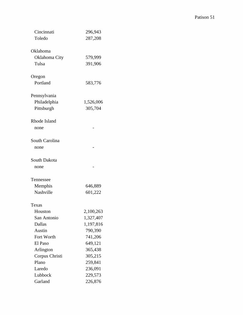
Patison 51

Cincinnati 296,943

Toledo 287,208

Oklahoma

Oklahoma City 579,999

Tulsa 391,906

Oregon

Portland 583,776

Pennsylvania

Philadelphia 1,526,006

Pittsburgh 305,704

Rhode Island

none -

South Carolina

none -

South Dakota

none -

Tennessee

Memphis 646,889

Nashville 601,222

Texas

Houston 2,100,263

San Antonio 1,327,407

Dallas 1,197,816

Austin 790,390

Fort Worth 741,206

El Paso 649,121

Arlington 365,438

Corpus Christi 305,215

Plano 259,841

Laredo 236,091

Lubbock 229,573

Garland 226,876

Patison 52

Irving 216,290

Utah

none -

Vermont

none -

Virginia

Virginia Beach 437,994

Norfolk 242,803

Chesapeake 222,209

Richmond 204,214

Washington

Seattle 608,660

Spokane 208,916

West Virginia

none -

Wisconsin

Milwaukee 594,833

Madison 233,209

Wyoming

none -

Patison 53

Appendix B: Election Sources

City Source Type

Alabama

Birmingham city

Montgomery city & county

Alaska

Anchorage city

Arizona

Phoenix city

Tucson city

Mesa city & county

Chandler county

Glendale county

Scottsdale county

Gilbert county

Arkansas

none -

California

Los Angeles city

San Diego city

San Jose county

San Francisco city

Fresno county

Sacramento county

Long Beach city

Oakland county

Bakersfield county

Anaheim county

Santa Ana county

Riverside city & county

Stockton county

Chula Vista city & county

Fremont county

Patison 54

Irvine county

San Bernardino county

Modesto county

Colorado

Denver city

Colorado Springs city

Aurora city & state

Connecticut

none -

Delaware

none -

District of Columbia

Washington city

Florida

Jacksonville city & county

Miami county

Tampa county

St. Petersburg county

Orlando city & county

Hialeah county

Georgia

Atlanta county

Hawaii

Honolulu county

Idaho

Boise county

Illinois

Chicago city

Indiana

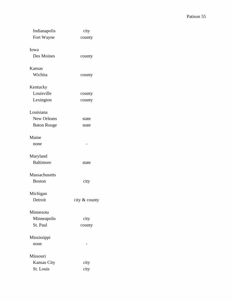
Patison 55

Indianapolis city

Fort Wayne county

Iowa

Des Moines county

Kansas

Wichita county

Kentucky

Louisville county

Lexington county

Louisiana

New Orleans state

Baton Rouge state

Maine

none -

Maryland

Baltimore state

Massachusetts

Boston city

Michigan

Detroit city & county

Minnesota

Minneapolis city

St. Paul county

Mississippi

none -

Missouri

Kansas City city

St. Louis city

Patison 56

Montana

none -

Nebraska

Omaha county

Lincoln city & county

Nevada

Las Vegas county

Henderson county

Reno county & state

North Las Vegas county

New Hampshire

none -

New Jersey

Newark county

Jersey City county

New Mexico

Albuquerque city & county

New York

New York City city

Buffalo county

Rochester county

North Carolina

Charlotte state

Raleigh state

Greensboro state

Winston-Salem state

Durham state

Fayetteville state

North Dakota

none -

Patison 57

Ohio

Columbus county

Cleveland county

Cincinnati county

Toledo county

Oklahoma

Oklahoma City state

Tulsa state

Oregon

Portland city & county

Pennsylvania

Philadelphia city

Pittsburgh county

Rhode Island

none -

South Carolina

none -

South Dakota

none -

Tennessee

Memphis county

Nashville city

Texas

Houston city & county

San Antonio city & county

Dallas county

Austin city & county

Fort Worth city & county

El Paso county

Arlington city & county

Patison 58

Corpus Christi county

Plano county

Laredo city

Lubbock county

Garland county

Irving city & county

Utah

none -

Vermont

none -

Virginia

Virginia Beach city & state

Norfolk city

Chesapeake city & state

Richmond state

Washington

Seattle city & county

Spokane county

West Virginia

none -

Wisconsin

Milwaukee city

Madison county

Wyoming

none -

Patison 59

Works Cited

Adams, J. (1776). Thoughts on Government. Thoughts on Government. Philadelphia, PA: John

Dunlap.

Alford, R. R., & Lee, E. C. (1968). Voting Turnout in American Cities. American Political

Science Review, 62(3), 796-813.

Alford, R. R., & Scoble, H. M. (1965). Political and Socioeconomic Characteristics of American

Cities. In Municipal Year Book. Chicago, IL: International City Managers’ Association.

Bullock, C. S. (1990). Turnout in Municipal Elections. Review of Policy Research, 9(3), 539-49.

Carr, J. B., & Tavares, A. F. (2014). City Size and Political Participation in Local Government:

Reassessing the Contingent Factors of Residential Location Decisions Within Urban

Regions. Urban Affairs Review, 50(2), 269-302.

Goodnow, F. J. (1908). City Government in the United States. New York, NY: The Century Co.

Hajnal, Z. L. (2010). America's Uneven Democracy: Race, Turnout, and Representation in City

Politics. Cambridge, United Kingdom: Cambridge University Press.

Hajnal, Z. L., & Lewis, P.G. (2003). Municipal Institutions and Voter Turnout in Local

Elections. Urban Affairs Review, 38(5), 645-68.

Hajnal, Z. L., Lewis, P.G., & Louch, H. (2002). Municipal Elections in California: Turnout,

Timing, and Competition. San Francisco, CA: Public Policy Institute of California.

Hajnal, Z. L., & Trounstine, J. (2005). Where Turnout Matters: The Consequences of Uneven

Turnout in City Politics. Journal of Politics, 67(2), 515-35.

Kaufmann, K. M. (2004). The Urban Voter: Group Conflict and Mayoral Voting Behavior in

Major Cities. Ann Arbor, MI: University of Michigan Press.

Kelleher, C. A., & Lowery, D. (2009). Central City Size, Metropolitan Institutions and Political

Participation. British Journal of Political Science, 39(1), 59-92. Kessel, J. H. (1962). Governmental Structure and Political Environment: A Statistical Note about

American Cities. American Political Science Review, 56(3), 615-20.

Mcdaniel, J. A. (2016). Writing the Rules to Rank the Candidates: Examining the Impact of

Instant-Runoff Voting on Racial Group Turnout in San Francisco Mayoral Elections.

Journal of Urban Affairs, 38(3), 387-408.

Patison 60

Morlan, R. L. (1984). Municipal vs. National Election Voter Turnout: Europe and the United

States. Political Science Quarterly, 99(3), 457-70.

Oliver, J. E. (2000). City Size and Civic Involvement in Metropolitan America. American

Political Science Review, 94(2), 361-73.

Oliver, E. J., Ha, S. E., & Callen, Z. (2012). Local Elections and the Politics of Small-Scale

Democracy. Princeton, NJ: Princeton University Press.

Rolfe, M. (2012). Voter Turnout: A Social Theory of Political Participation. New York, NY:

Cambridge University Press.

Schnore, L. F., & Alford, R. R. (1963). Forms of Government and Socioeconomic

Characteristics of Suburbs. Administrative Science Quarterly, 8(1), 1-17.

Verba, S., Schlozman, K., & Brady, H. (1995). Voice and Equality. Cambridge, MA: Harvard

University Press.

Wolfinger, R. E., & Rosenstone, S. J. (1980). Who Votes? New Haven, CT: Yale University

Press.

Wood, C. (2002). Voter Turnout in City Elections. Urban Affairs Review, 38(2), 209-31.