Why do Education Expenditures fail to decrease child labor ...cerdi.org/uploads/sfCmsContent/html/199/Rota_Grigoriou.pdf · Why do Education Expenditures fail to decrease child labor?

Why do Education Expenditures fail to decrease child

labor? Impact and Optimal Composition of Social

Expenditures

Christopher Grigoriou∗ and Grégoire Rota Graziosi†

CERDI-CNRS, Université d’Auvergne.

May 17, 2005

Abstract

Relying on a theoretical model where child labor results from a risky choice

between working or schooling, this paper aims at studying why do education ex-

penditures fail to decrease child labor. We suggest an optimal composition of social

expenditures which minimizes child labor for a given government’s budget. A com-

plementarity between social expenditures is established. The unbalanced structure

of the social expenditures favourable to the education expenditures in the poor

countries seems therefore not to be consistent. These hypothesis are tested with

econometric panel data over 81 developing countries. Our statements, which are

validated, shed light on the need to reconsider the conventional wisdom viewing

public health and education expenditures as substitutes.

Keywords: Child Labor, Education Expenditures, Health Expenditures.

JEL classification: J20, K31, D60.

∗CERDI-CNRS, Université d’Auvergne. Email: [email protected]†CERDI-CNRS, Université d’Auvergne. Email: [email protected]

1

1 Introduction

While achieving schooling for all by 2015 is one of the millenium development goals as

defined by the United Nations, the International Labor Office estimates that in 2000 211

million children aged 5 to 14 work full-time, 48 million of which living in subsaharan

Africa, 127 million others in the region Asia-Pacific, 73 million of them being less than

10 years old (International Labour Office (2002)). Besides the rule of law and the

issue of the ban of child labor (see Dessy and Pallage (2005)), it is henceforth crucial

to understand how the governments can act to reduce child labor through the social

expenditures.1

Special attention has to be paid to education expenditures, expected to impact di-

rectly child labor through an increase in the education return. However, among others,

Patrinos and Psacharopoulos (2004) enhance that public education has severely failed

in increasing return to education, due to "uneconomic policies", while Schultz (1999)

argues that education only benefit to an elite in developping countries. Hence, public

education expenditures would not provide the conditions for strong decreases in child

labor. In that paper, we attempt to develop a possible reason for these "uneconomic

policies", depending on the share of each kind of social expenditures on the whole so-

cial spending (we resume the social expenditures to education and health ones), arguing

that due to their complementarity, health and education expenditures have to be studied

jointly.

On the empirical ground, the distribution of public expenditures between education

and health in developing countries is much more favourable to the former as emphasized

by Burgess and Stern (1993).2 Actually,a structural difference between poor and rich

countries seems to emerge with regard to the relative weight of each kind of spending:

the poorer the countries, the more they invest on education related to health, which can1 Our focus hence relies at the crossroad of the child labor economic analysis (for a survey, see Basu

(1999)) and of the public spending efficiency (in particular that of health and education).2See their Table 1 and comments, p. 765-6.

2

be illustrated with Figure 1.

Insere Figure 1 here

Whereas education and health expenditures are often agregated as a composite so-

cial spending in the literature (see for instance Devarajan, Swaroop, and Zou (1996)),

assuming the same impact for the both policies, we specify one transmission channel for

each of them. A simple theoretical model is developped, where child labor results from

a household’s choice between working and schooling. This household’s decision corre-

sponds to an intertemporal trade-off or to a risky choice. In this last interpretation, we

consider the child labor as the riskless asset and the child education as the risky one.

This is crucial since the risk aversion is often expected to be all the higher as individuals

are poor. In our framework, each type of public expenditure influes on the household’s

choice through a particular way. This choice depends both on the return and on the risk

of investing in education. Education spending is expected to increase the return on (the

investment in) education, while health spending is supposed to reduce the risk of this

investment by improving the health status, proxying the preference for present . More-

over, our approach falls under the economic analysis on longevity where the likelihood

of survival for children determine education and fertility choices (see Ehrlich and Lui

(1991)).

We suggest an optimal composition of social expenditures which minimizes child

labor for a given government’s budget. A complementarity between social expenditures

is established. The unbalanced structure of the social expenditures favourable to the

education expenditures in the poor countries seems therefore not to be consistent. These

hypothesis are tested with econometric panel data over 81 developing countries. Our

statements, which are validated, shed light on the need to reconsider the conventional

wisdom viewing public health and education expenditures as substitutes.

3

The plan of the paper is as follows. Section 2 sets out the basic assumptions of our

analysis. Section 3 studies the theoretical effects of the two kinds of policy (health and

education) on the child labor. Section 4 provides some empirical validations. Section 5

summarizes the discussion and offers a few concluding comments.

2 Theoretical Framework

Our theoretical framework relies on Baland and Robinson (2000) and on Dessy and Pal-

lage (2001).3 Following Strulik (2004), we go further the formers, taking into account

the risk in the parental decision to make the children work, including child mortality in

the parental decision of child labor. However, we enlarge Strulik (2004) analysis by em-

phasizing the effects of public health and education spending. Similarly to Chakraborty

and Das (2004) who establish a positive relationship between parental health and chil-

dren’s education, we set a link between child mortality and child labor. But, while adult

mortality is in Chakraborty and Das (2004) a function of private health expenditures,

child mortality is in our model explained by the public health expenditures.

The optimization process concerns the child time allocation between working and

schooling. Children own one unit of time which might be allocated to school (γ ∈ [0, 1])or to work (1− γ). This relevant choice is made by the parents since the children are

supposed to be too young to make rational (schooling) decisions (see Glomm (1997)).

If we consider children as an asset4, the child time allocation between work and school

is a risky investment for the household. The parental choice is then a portfolio deci-

sion, between a riskless investment (child labor) and a risky but more profitable one

(schooling).

We consider a two-period economy (t = 1, 2) with one single consumption good.

3Given the available data, we do not develop an overlapping generations model.4Dasgupta (1995) argues that "in poor countries children are also useful as income-earning assets."

(p. 1895)

4

There is no discount of the future by the agents. At the first period, the household consists

of one working adult, the parent (p), and of one child (c); at the second period, there

are two adults (p and a), each of them controlling his own income. Following Baland

and Robinson (2000) or Dessy and Pallage (2001), we assume separable preferences,

denoted U(.), a normalization to zero of child consumption and some altruism from

parents to their children (one-side altruism). We denote Wp, the parental utility, as

Wp

¡c1p, c

2p,Wc (cc)

¢, where c1p, c

2p and Wc (cc) are respectively the consumption of first

period, the consumption of second period and the child utility Wc depending on cc, the

child consumption of second period. It yields:

Wp

¡c1p, c

2p,Wc (cc)

¢ ≡ U¡c1p¢+ U

¡c2p¢+ φδWc (cc) , (1)

where U and Wc are strictly increasing and concave functions. The parameter δ is

the degree of altruism, which induces the intergenerational link. The parameter φ is

the probability of child survival or the preference for the present.5 Contrary to ?, this

probability is certain and known. Its increase is equivalent to a decrease in the preference

for the present. In the next section, this parameter (φ) will be endogenously determined

by the public health expenditures.

In the lack of saving and borrowing, consumption equalizes the available income at

each period. At the first one, the household’s income corresponds to the sum of the

parental wage, denoted w, and of the child(ren) earning, (1− γ)wc, which is the child’s

time spent at work (1 − γ) valued at the child’s wage rate (wc). At the second period,

parents still earn w.6 The remunerations of the children when adults depend on their

education level: a working child will earn the same wage as his parents (w), while an

5Chakraborty (2004) and Chakraborty and Das (2004) also consider individual health status as anexplanatory factor of the discount rate.

6The assumption that parent are still working at the second stage has no impact on the equilibriumchild labor’s level. Alternatives would be to suppose that parent died or does not work anymore at thesecond period.

5

educated child will be a skilled worker, whom wage is denoted ws. It yields:

c1p ≡ w + (1− γ)wc, c2p ≡ w, cc ≡ (1− γ)w + γws. (2)

We focus now on the labor demand side. We ignore the depreciating effect of the child

labor on the parental wage as analysed by Basu and Van (1998). We assume a perfect

competition between firms, which induces an equalization of the wages to the marginal

productivity of the different kind of workers. More precisely, we consider that the child

productivity is a fraction d (d < 1) of the parent’s productivity. The skilled worker, i.e.

the former educated child, has a productivity that increases with the level of education,

denoted e, which will be considered endogenous in the next section. Hence, these labor

market conditions involve:

wc = dw, wa = ew. (3)

Substituting (2) and (3) in (1), the solution of the parent’s maximization program,

denoted γ∗, is given by:

γ∗ ∈ argmaxγ∈[0,1]

{Wp (w + (1− γ) dw,w,Wc ((1− γ)w + γew))} .

If an interior solution exists, the First Order Condition (FOC) is equivalent to:7

−dU 0 ((1 + d− dγ∗)w) + φδ (e− 1)W 0c ((1− γ∗ + γ∗e)w) = 0,

which is equivalent to:φδ (e− 1)

d=

U 0¡c1∗p¢

W 0c (c

∗c)≡ f (γ∗; .) . (4)

7The Second Order Condition (SOC) is valid:

w2cU00 c1p + φδ (w − wa)

2W 00c (cc) < 0.

6

where we denote c∗c ≡ (1− γ∗ + γ∗e)w and c1∗p ≡ (1 + (1− γ∗) d)w. The equilibrium

level of child schooling time (γ∗) is determined by the equalization of the intertemporal

consumption Marginal Rate of Substitution (MRS) to the "actualized" ratio of the gain

of education investment (e − 1) on what can be interpreted as the opportunity cost ofeducation (d). Indeed, even without any private cost of education, educating children

remains costly for parents, due to the fact that the child time is valuable on labor market

(see Rosenzweig (1990)).

By inspection of (4) it is immediate that ∂f(γ∗;.)∂γ∗ > 0.8 We might also have two

corner solutions. There is no school (γ∗ = 0) if and only if:

∀γ ∈ [0, 1] , f (γ; .) >φδ (e− 1)

d⇔ f (0; .) =

U 0 ((1 + d)w)

W 0c (w)

>φδ (e− 1)

d

⇔ e < 1 +d

φδ

U 0 ((1 + d)w)

W 0c (w)

Similarly, there is no child labor (γ∗ = 1) if and only if:

∀γ ∈ [0, 1] , f (γ; .) <φδ (e− 1)

d⇔ f (1; .) =

U 0 (w)W 0

c (ws)<

φδ (e− 1)d

⇔ d < φδ (e− 1)W0c (ew)

U 0 (w)

There is no child labor (respectively no education) when the child wage, wc, or the return

to education, e, (respectively the wage of skilled workers, ws, or the child productivity,

d) is sufficiently low. Consider the partial inverse of f (.) with respect to γ∗, which we

shall denote by ψ, where ψ (f (γ∗;w, d, e) ;w, d, e) = γ∗. We then have the following

Proposition:8

∂(U 0(c1p(γ∗)))

∂γ∗ = −wcU00 c1p (γ

∗) > 0∂(W 0

c(cc(γ∗)))∂γ∗ = (wa − w)W 00

c (cc (γ∗)) < 0

⇒ ∂fγ∗ (γ∗; .)

∂γ∗=

∂U0(c1p(γ∗))W 0c(cc(γ

∗))

∂γ∗> 0.

7

Proposition 1 The household’s optimal decision is given by:

γ∗ ≡

1, if d < φδ (e− 1) W 0

c(ew)U 0(w)

0, if e < 1 + dφδ

U 0((1+d)w)W 0c(w)

ψ³φδ(e−1)

d ;w, d, e´, otherwise

(5)

An implicit assumption has been set here: when the parents choose the schooling

time of their children, they do not integrate the influence of this decision on the future

wage of the skilled worker. Indeed, we consider that the parents are numerous enough

to take the wages as given. In other words, at the decentralized equilibrium, households

take as given the return to education.

3 Public Intervention and optimal policy

In this section, we focus on two kinds of public incentives to ensure a decrease in the

child labor: public education and public health expenditures (respectively denoted E

and H). We develop one specific mecanism for each policy: public education spending

increases the return of investment in education, while health spending reduces the risk

of this investment by improving the health status. However, the government’s balanced

budget constraint involves a relationship between the two kind of public expenditures.

We first present the effect of each public spending on child labor. Then, we develop the

consequences of taxation on our results.

According to the literature, the impact of public health spending (H) on health

outcome is questionable. The following studies, proxying health status by infant or

child mortality, result in different appreciation of this impact. On one hand, Anand

and Ravallion (1993) show a positive impact.9 On the other hand, Filmer, Hammer,

and Pritchett (2000) find no significant impact of public spending on health status on

a cross-section over 100 countries. Finally, Bidani and Ravallion (1997) as well as

Gupta, Verhoeven, and Tiongson (2001) emphasize a positive impact on health care of9However, the econometric validation of this study relies on only 22 observations.

8

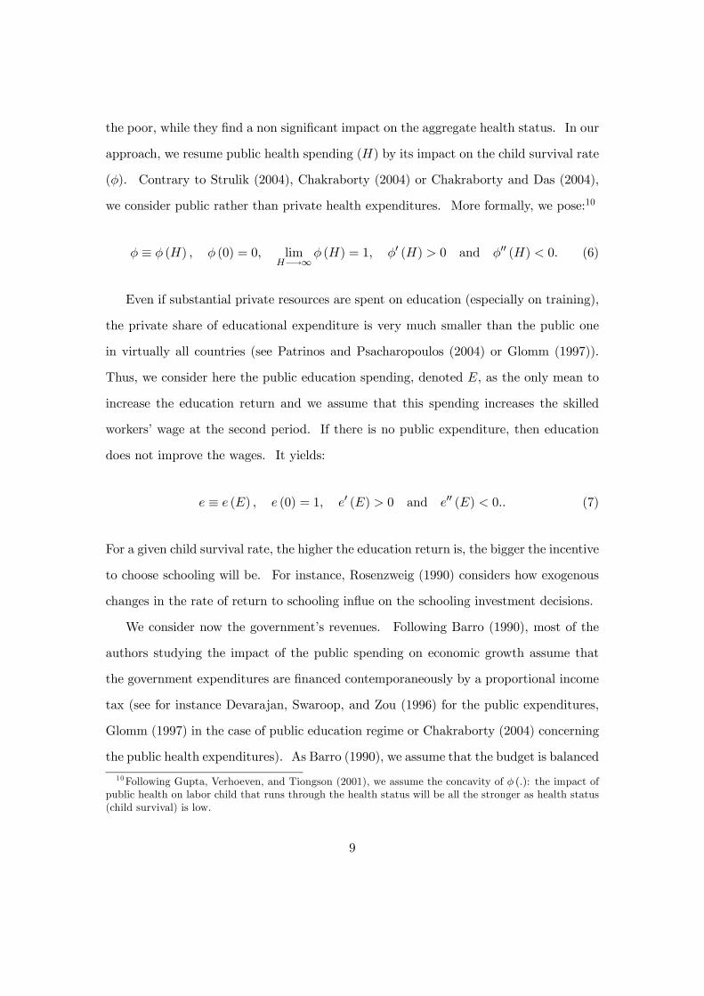
the poor, while they find a non significant impact on the aggregate health status. In our

approach, we resume public health spending (H) by its impact on the child survival rate

(φ). Contrary to Strulik (2004), Chakraborty (2004) or Chakraborty and Das (2004),

we consider public rather than private health expenditures. More formally, we pose:10

φ ≡ φ (H) , φ (0) = 0, limH−→∞

φ (H) = 1, φ0 (H) > 0 and φ00 (H) < 0. (6)

Even if substantial private resources are spent on education (especially on training),

the private share of educational expenditure is very much smaller than the public one

in virtually all countries (see Patrinos and Psacharopoulos (2004) or Glomm (1997)).

Thus, we consider here the public education spending, denoted E, as the only mean to

increase the education return and we assume that this spending increases the skilled

workers’ wage at the second period. If there is no public expenditure, then education

does not improve the wages. It yields:

e ≡ e (E) , e (0) = 1, e0 (E) > 0 and e00 (E) < 0.. (7)

For a given child survival rate, the higher the education return is, the bigger the incentive

to choose schooling will be. For instance, Rosenzweig (1990) considers how exogenous

changes in the rate of return to schooling influe on the schooling investment decisions.

We consider now the government’s revenues. Following Barro (1990), most of the

authors studying the impact of the public spending on economic growth assume that

the government expenditures are financed contemporaneously by a proportional income

tax (see for instance Devarajan, Swaroop, and Zou (1996) for the public expenditures,

Glomm (1997) in the case of public education regime or Chakraborty (2004) concerning

the public health expenditures). As Barro (1990), we assume that the budget is balanced

10Following Gupta, Verhoeven, and Tiongson (2001), we assume the concavity of φ (.): the impact ofpublic health on labor child that runs through the health status will be all the stronger as health status(child survival) is low.

9

on the first period, i.e. that at this period, the total collected tax equalizes the public

spending. However, income tax can not be considered as the representative tax of the

fiscal system in developing countries (see Burgess and Stern (1993) or Chambas (2004)).

According to Alm and Wallace (2004), it seems "unlikely" that these countries are able

to manage a broad-based individual income tax. This is why we consider a per capita

tax (more accurately, a tax per household), denoted T .11 The budget constraint is

given by: T = E +H. The household’s objective function becomes:

W (γ,E,H, T ;w, d) = U ((1 + d− γd)w − T )+U (w)+ δφ (H)Wc ((1− γ + γe (E))w) .

(8)

The FOC is then:12

−dU 0 ¡£1 + d− γT∗d¤w − T

¢+ δφ (H) (e (E)− 1)W 0

c

¡£1− γT∗ + γT∗e (E)

¤w¢= 0,

(9)

where γT∗ is the solution in a per capita tax fiscal system. The FOC (9) is equivalent

to:δφ (H) (e (E)− 1)

d=

U 0¡c1∗p − T

¢W 0

c (c∗c)

It yields:

γT∗ =

1, if d < φ (H) δ (e (E)− 1) W 0

c(e(E)w)U 0(w)

0, if e (E) < 1 + dφ(H)δ

U 0((1+d)w)W 0c(w)

ψ³φ(H)δ(e(E)−1)

d ;w, dw, e (E)w´, otherwise

(10)

We consider now the government behavior whose goal is to raise the schooling in-

vestment (γT∗). We do not consider the coordination failures nor the time inconstency11Here, we differ from Glomm (1997) who assumes no taxation on child labor, since children are mostly

employed in the informal sector. Under his assumption, taxation will increase the relative child wagecompared to the parent’s wage, and thus will increase the incentives to child labor.12The SOC remains valid:

−d2w2U 00 ((1 + d− γ∗d)w) + δφ (H) (e (E)− 1)2W 00c ((1− γ∗ + γ∗e (E))w) < 0.

10

in the relationship between the government and the households. We denote α, the share

of the fiscal ressources allowed to education: E = αT and H = (1− α)T . We define

γT∗ (α, T ) the solution (10) with regard to α and T . Given the fiscal pressure (T ), the

optimal composition of public expenditures, denoted α∗, is the solution of the following

programm:

α∗ ≡ argmaxα∈[0,1]

γT∗ (α, T ) . (11)

The following Proposition resumes our results:

Proposition 2 Under a per capita tax, there exists an optimal composition of socialpublic spending between health and education (α∗) given by:

φ0 (α∗T ) (e ((1− α∗)T )− 1)+φ (α∗T ) e0 ((1− α∗)T )£γT∗ (e ((1− α∗)T )− 1)A (c∗c)− 1

¤= 0

(12)

Proof: See Appendix.

In order to be more conclusive, we specify our utility functions (U (.) and W (.))

from different forms. An approximation of expression ψ³φ(H)δ(e(E)−1)

d ;w, dw, e (E)w´

in (10) is given by a first order Taylor expansion of (9) with respect to γ at γ∗T :

−d £U 0 ((1 + d)w)− dwγ∗TU 00 ((1 + d)w)¤+φδ (e− 1) £W 0

c (w) + γ∗T (e− 1)wW 00c (w)

¤= 0.

Substituting E and H by their expression in terms of α and T allows to express the

interior solution:

γT∗ (α, T ) =dU 0 ((1 + d)w)− δφ (αT ) (e ((1− α)T )− 1)W 0

c (w)

whφ (αT ) δ (e ((1− α)T )− 1)2W 00

c (w) + d2U 00 ((1 + d)w)i . (13)

We illustrate proposition 2 using expression (13) with four specific functional forms

(logarithmic, CRRA, CARA and HARA).


11

Figure 2 shows how the optimal education investment (γT∗ (α, T )) varies according

to the composition of public expenditures (α ∈ [0, 1]) for different levels of fiscal pressure(T ). might be deduced from Figure 2. The parents optimal choice (γ∗ (α, T )) is initially

increasing and then decreasing, whatever the utility function is. We deduce that an

increase in the education expenditures, for a given budget (T ) will only be efficient

on the left (growing) side of the curve. On the contrary, beyond a certain investment in

education, any additional education expenditures that is at the expense of the health ones

is inefficient. Last, there may be an infinity of combination health-education ensuring

the elimination of child labor (see for instance on the figure γ∗ (α, 5) and γ∗ (α, 10) with

the logarithmic utility function).

Figure 3 illustrates the impact of the parental risk aversion on γ∗ (α, T ), depending

on both the level of tax pressure and the distribution of the social expenditures.


Even if trivial, given the assumptions of our model, this figure highlights the crucial role

of the parental risk aversion to send their children to school.

4 Econometric validation

The following table presents the correspondance of theoretical and empirical symbols.

Insere Table 1 here

Our estimates rely on panel data over 81 developing countries for three averaged 5 year

periods (1986-1990, 1991-1995, 1996-2000). The first assumption to be tested is the way

the trade-off between working and schooling is impacted by the preference for present,

proxied by the health status and measured by the child survival rate: an increase in

12

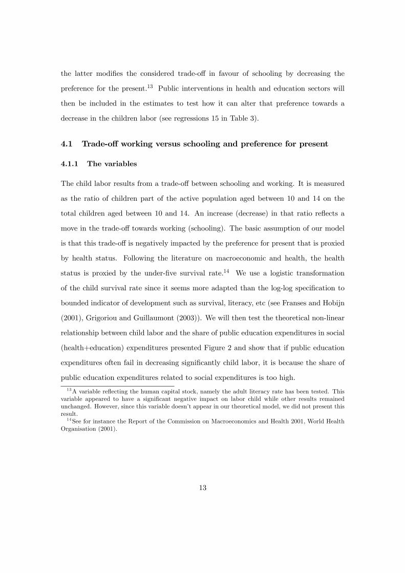
the latter modifies the considered trade-off in favour of schooling by decreasing the

preference for the present.13 Public interventions in health and education sectors will

then be included in the estimates to test how it can alter that preference towards a

decrease in the children labor (see regressions 15 in Table 3).

4.1 Trade-off working versus schooling and preference for present

4.1.1 The variables

The child labor results from a trade-off between schooling and working. It is measured

as the ratio of children part of the active population aged between 10 and 14 on the

total children aged between 10 and 14. An increase (decrease) in that ratio reflects a

move in the trade-off towards working (schooling). The basic assumption of our model

is that this trade-off is negatively impacted by the preference for present that is proxied

by health status. Following the literature on macroeconomic and health, the health

status is proxied by the under-five survival rate.14 We use a logistic transformation

of the child survival rate since it seems more adapted than the log-log specification to

bounded indicator of development such as survival, literacy, etc (see Franses and Hobijn

(2001), Grigoriou and Guillaumont (2003)). We will then test the theoretical non-linear

relationship between child labor and the share of public education expenditures in social

(health+education) expenditures presented Figure 2 and show that if public education

expenditures often fail in decreasing significantly child labor, it is because the share of

public education expenditures related to social expenditures is too high.

13A variable reflecting the human capital stock, namely the adult literacy rate has been tested. Thisvariable appeared to have a significant negative impact on labor child while other results remainedunchanged. However, since this variable doesn’t appear in our theoretical model, we did not present thisresult.14See for instance the Report of the Commission on Macroeconomics and Health 2001, World Health

Organisation (2001).

13

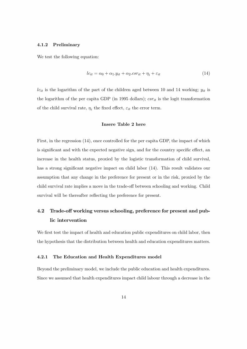
4.1.2 Preliminary

We test the following equation:

lcit = α0 + α1.yit + α2.csrit + ηi + εit (14)

lcit is the logarithm of the part of the children aged between 10 and 14 working; yit is

the logarithm of the per capita GDP (in 1995 dollars); csrit is the logit transformation

of the child survival rate, ηi the fixed effect, εit the error term.

Insere Table 2 here

First, in the regression (14), once controlled for the per capita GDP, the impact of which

is significant and with the expected negative sign, and for the country specific effect, an

increase in the health status, proxied by the logistic transformation of child survival,

has a strong significant negative impact on child labor (14). This result validates our

assumption that any change in the preference for present or in the risk, proxied by the

child survival rate implies a move in the trade-off between schooling and working. Child

survival will be thereafter reflecting the preference for present.

4.2 Trade-offworking versus schooling, preference for present and pub-

lic intervention

We first test the impact of health and education public expenditures on child labor, then

the hypothesis that the distribution between health and education expenditures matters.

4.2.1 The Education and Health Expenditures model

Beyond the preliminary model, we include the public education and health expenditures.

Since we assumed that health expenditures impact child labour through a decrease in the

14

preference for the present, health expenditures is not only included additively (heit) but

also interacted with the variable csrit. Hence, the impact of health expenditures on child

labour will be all the stronger as the preference for the present (the child survival rate)

will be high (low). Then we add the public health expenditures variable, the impact of

which is expected negative. However, given the litterature, a non-significant coefficient

would not be very surprising.

The following model is to be tested.:

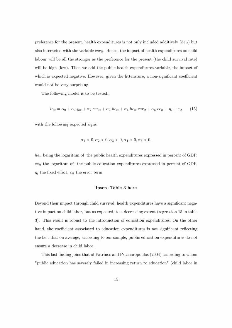
lcit = α0 + α1.yit + α2.csrit + α3.heit + α4.heit.csrit + α5.eeit + ηi + εit (15)

with the following expected signs:

α1 < 0, α2 < 0, α3 < 0, α4 > 0, α5 < 0,

heit being the logarithm of the public health expenditures expressed in percent of GDP,

eeit the logarithm of the public education expenditures expressed in percent of GDP,

ηi the fixed effect, εit the error term.

Insere Table 3 here

Beyond their impact through child survival, health expenditures have a significant nega-

tive impact on child labor, but as expected, to a decreasing extent (regression 15 in table

3). This result is robust to the introduction of education expenditures. On the other

hand, the coefficient associated to education expenditures is not significant reflecting

the fact that on average, according to our sample, public education expenditures do not

ensure a decrease in child labor.

This last finding joins that of Patrinos and Psacharopoulos (2004) according to whom

"public education has severely failed in increasing return to education" (child labor in

15

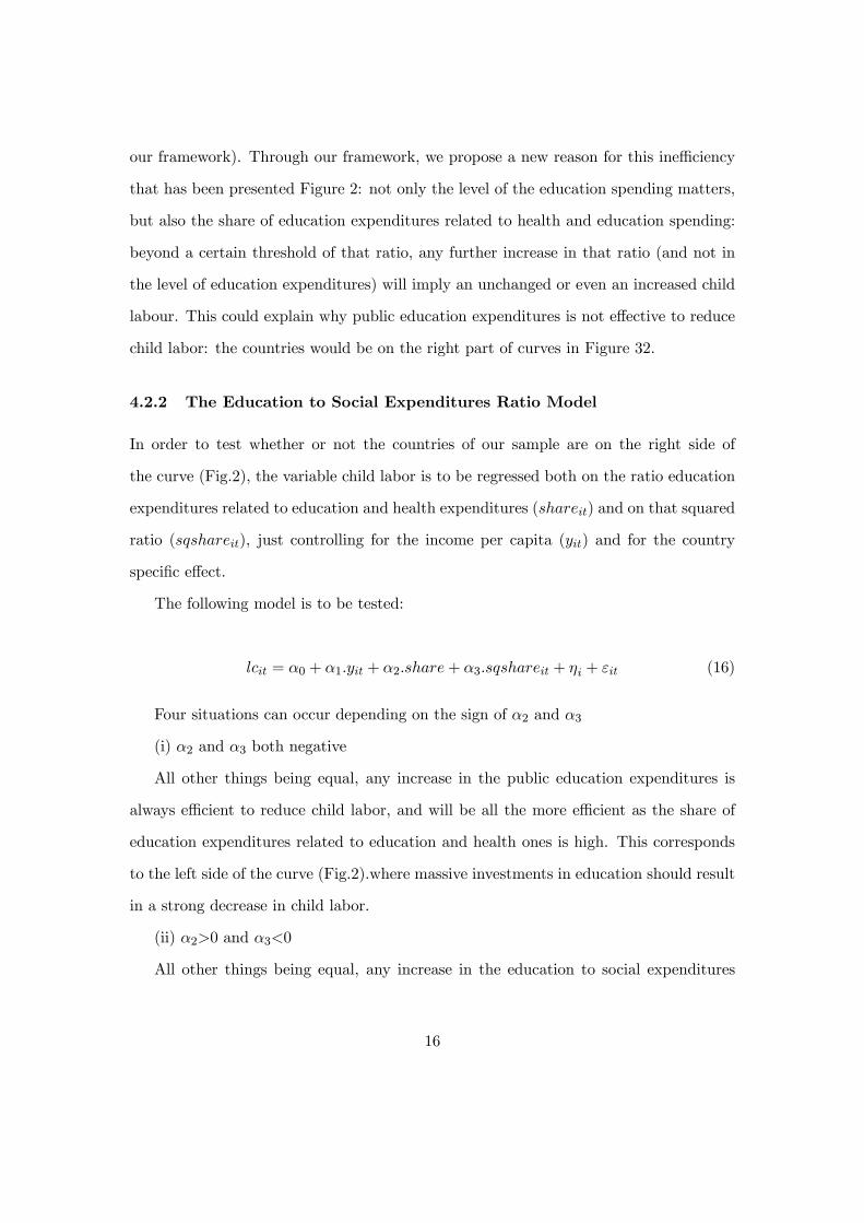
our framework). Through our framework, we propose a new reason for this inefficiency

that has been presented Figure 2: not only the level of the education spending matters,

but also the share of education expenditures related to health and education spending:

beyond a certain threshold of that ratio, any further increase in that ratio (and not in

the level of education expenditures) will imply an unchanged or even an increased child

labour. This could explain why public education expenditures is not effective to reduce

child labor: the countries would be on the right part of curves in Figure 32.

4.2.2 The Education to Social Expenditures Ratio Model

In order to test whether or not the countries of our sample are on the right side of

the curve (Fig.2), the variable child labor is to be regressed both on the ratio education

expenditures related to education and health expenditures (shareit) and on that squared

ratio (sqshareit), just controlling for the income per capita (yit) and for the country

specific effect.

The following model is to be tested:

lcit = α0 + α1.yit + α2.share+ α3.sqshareit + ηi + εit (16)

Four situations can occur depending on the sign of α2 and α3

(i) α2 and α3 both negative

All other things being equal, any increase in the public education expenditures is

always efficient to reduce child labor, and will be all the more efficient as the share of

education expenditures related to education and health ones is high. This corresponds

to the left side of the curve (Fig.2).where massive investments in education should result

in a strong decrease in child labor.

(ii) α2>0 and α3<0

All other things being equal, any increase in the education to social expenditures

16

ratio will first (for the low value of the ratio) be inefficient to decrease child labor but

beyond a certain threshold it will become increasingly efficient. This would correspond

to an inversed U-curve, which is at the opposite of the assumptions of our theoretical

model.

(iii) α2<0 and α3>0

All other things being equal, any increase in the education to social expenditures

ratio will first (for the low value of the ratio) be efficient to decrease child labor (left

side of the curve) but beyond a certain threshold it will become increasingly efficient.

This would correspond to the U-curve following our theoretical model. It means that

beyond a certain threhold, the education investment has to be accompanied by health

investments in order to benefit from the complementarities of this two public goods.

(iv) α2 and α3 both positive

All other things being equal, any increase in the public education expenditures is

always inefficient to reduce child labor. This corresponds to the right side of the curve

(Fig.2).where education expenditures should be accompanied by massive invest in health:

decreasing the preference for the present, health investments would ensure a context more

favorable to education investment.

Insere Table 4 here

Estimate of 16 result in α2 and α3 both positive and significant. According to (iv) it

means that our developing countries sample is on average on the right side of the curve.

We are then able to provide an explanation to the ineffectiveness of public education

expenditures with regard to the child labor decrease: it is not only the level of education

expenditures that matters, but also the share of education expenditures in social spend-

ing. Beyond a certain threshold, it is useless to increase education expenditures if this is

not accompanied by health expenditures that will ensure a decrease in the preference for

17

the the present (risk of the investment in education), implying a context more favorable

to education investments (from the parents).

4.3 Econometric discussion

4.3.1 Fixed effect estimate and serial correlation

The use of panel data econometric with the introduction of country specific effects (ηi)

allows us to control for unobservable constant heterogeneity between these countries.

Moreover, while it is often assumed that most of the observed serial correlation is domi-

nated by the presence of this country specific effect in the composite errors uit = ηi+εit,

(the potential serial correlation being then eliminated by the within transformation),

Wooldridge (2002) highlights that there can be serial dependence in the residual term

εit, the fixed effect standard errors being in that case very misleading. Following Drukker

(2003), we specify Newey-West standard errors for fixed effect models, to face any po-

tential problem of serial correlation that would bias the inference: it corrects both the

heteroskedastic and the autocorrelated structure of the error.

4.3.2 Reverse causality

One could argue that explaining child labor by education expenditures may induce a

reverse causality leading to an endogeneity bias since the level of education expenditures

is likely to be all the higher (lower) as child labor is rare (important). However it seems

obvious that in the context of developing countries, i.e. in scarcity economies, and

moreover on social questions as education and health are, the causality goes from the

supply side and not from the demand one.

18

5 Political implications and concluding remarks

This paper aims at analysing the effects of education and health expenditures on child

labor. The household’s choice to have their child(ren) working or schooling can be viewed

either as an intertemporal trade-off or as a risky choice, education being in that case a

risky investment. In this framework, each type of public spending influes on the indi-

vidual trade-off through a particular way: the education spending increases the return

of education, while the health spending reduces the risk of children death. Our theoret-

ical model emphasizes that these expenditures can not be considered systematically as

substitute, what is validated by the empirical findings.

References

Alm, J., and S. Wallace (2004): “Can Developing Countries Impose an In-

dividual Income Tax?,” Andrew Young School of Policy Studies, available at

http://aysps.gsu.edu/publications/2004/040801develop.htm.

Anand, S., and M. Ravallion (1993): “Human Development in Poor Countries: On

the Role of the Private Incomes and Public Services,” Journal of Economic Perspec-

tives, 7, 133—150.

Baland, J.-M., and J. A. Robinson (2000): “Is Child Labor Inefficient?,” Journal of

Political Economy, 108, 663—679.

Barro, R. J. (1990): “Government Spending in a Simple Model of Endogenous

Growth,” Journal of Political Economy, 98, 103—125.

Basu, K. (1999): “Child Labor: Cause, Consequence, and Cure, with Remarks on

International Labor Standards,” Journal of Economic Literature, 37, 1083—1119.

19

Basu, K., and P. H. Van (1998): “The Economics of Child Labor,” American Eco-

nomic Review, 88, 412—427.

Bidani, B., and M. Ravallion (1997): “Decomposing Social Indicators Using Distri-

butional Data,” Journal of Econometrics, 77, 125—139.

Burgess, R., and N. Stern (1993): “Taxation and Development,” Journal of Eco-

nomic Literature, 31(2), 762—830.

Chakraborty, A. (2004): “Endogeneous Lifetime and Economic Growth,” Journal of

Economic Theory, 116, 119—137.

Chakraborty, S., and M. Das (2004): “Mortality, Fertility and Child Labor,” Eco-

nomics Letters, forthcomming.

Chambas, G. (2004): "L’Afrique au Sud du Sahara. Mobiliser des ressources fiscales

pour le développement. Economica, Paris.

Dasgupta, P. (1995): “The Population Problem: Theory and Evidence,” Journal of

Economic Literature, 33, 1879—1902.

Dessy, S., and S. Pallage (2001): “Child Labor and Coordination Failure,” Journal

of Development Economics, 65, 469—476.

Dessy, S. E., and S. Pallage (2005): “A Theory of the Worst Forms of Child Labour,”

Economic Journal, 115(127), 68—87.

Devarajan, S., V. Swaroop, and H. Zou (1996): “The Composition of Public Ex-

penditure and Economic Growth,” Journal of Monetary Economics, 37, 313—344.

Drukker, D. (2003): “Testing for Serial Correlation in Linear Panel-Data Models,”

Stata Journal, 3, 168—177.

20

Ehrlich, I., and F. T. Lui (1991): “Intergenerational Trade, Longevity, and Economic

Growth,” Journal of Political Economy, 99(5), 1029—59.

Filmer, D., J. Hammer, and L. Pritchett (2000): “Weak Links in the Chain: A

Diagnosis of Health Policy in Poor Countries,” World Bank Research Observer, 15,

199—224.

Franses, P., and B. Hobijn (2001): “Are Living Standard Converging?,” Structural

change and Economic Dynamics, 12, 171—200.

Glomm, G. (1997): “Parental Choice of Human Capital Investment,” Journal of De-

velopment Economics, 53, 99—114.

Grigoriou, C., and P. Guillaumont (2003): “A Dynamic Child Survival Function:

Natural Convergence and Economic Policy,” Etudes et Documents, CERDI.

Gupta, S., M. Verhoeven, and E. Tiongson (2001): “Public Spending on Health

Care and the Poor,” IMF Working Paper, WP/01/127.

International Labour Office (2002): Every Child Counts- New Global Estimates

on Child Labour,. International Program on the Elimination of Child Labour (IPEC).

Patrinos, H.-A., and G. Psacharopoulos (2004): “Returns to Investment in Edu-

cation: A Further Updatde„” Education Economics, 12, 111—134.

Rosenzweig, M. (1990): “Economic Growth and Human Capital Investments: Theory

and Evidence,” Journal of Political Economy, 53, 202—211.

Strulik, H. (2004): “Child Mortality, Child Labour, and Economic Development,”

Economic Journal, 114, 547—568.

Wooldridge, J. (2002): Econometric Analysis of Cross-Section and Panel Data. MIT

Press, Cambridge, MA.

21

World Bank (2004): the World Development Indicators 2004, CD-ROM.

World Health Organisation (2001): Macroeconomics and Health: In-

vesting in Health for Economic Development. Geneva, available at

http://www.cid.harvard.edu/cidcmh/CMHReport.pdf.

A Appendix:

A.1 Proof of Proposition 2

The programm is α∗ ≡ argmaxα∈[0,1]

γT∗ (α, T ) . By applying the envelop theorem to (9) with

respect to α, it yields:

∂γT∗ (α, T )∂α

= −Tδφ0 (αT ) (e ((1− α)T )− 1)W 0

c (c∗c)− Tδφ (αT ) e0 ((1− α)T )W 0

c (c∗c)

−γT∗Tδφ (αT ) e0 ((1− α)T ) (e ((1− α)T )− 1)W 00c (c

∗c)

SOC,

Thus, from the FOC of (11), a solution, denoted α∗, is given implitly by:

∂γT∗ (α, T )∂α

= 0⇔ φ0 (α∗T ) (e ((1− α∗)T )− 1)+φ (α∗T ) e0 ((1− α∗)T )

£γT∗ (e ((1− α∗)T )− 1)A (c∗c)− 1

¤= 0

where A (.) denotes the Arrow-Pratt abolute risk aversion measure. Indeed, since thechild is not a decision maker (he is considered as too young to choose to invest inschooling), we express our conditions in term of parental risk aversion with respect tothe children consumption at the second period, denoted A (c∗c). We have:

∂W¡c1p, c

2p,Wc (cc)

¢∂cc

= δφ (H)W 0 (cc) ,∂2W

¡c1p, c

2p,Wc (cc)

¢∂c2c

= δφ (H)W 00 (cc) ,

Ac (cc) = A (cc) , where A (cc) ≡ −∂W(c1p,c2p,Wc(cc))

∂cc

∂2W(c1p,c2p,Wc(cc))∂c2c

The SOC is:∂2γT∗ (α, T )

∂α2< 0⇔ ∂FOC

∂α< 0,

22

where FOC correspond to the expression of ∂γT∗(α,T )∂α .

∂FOC∂α =

Tφ00 (α∗T ) (e ((1− α∗)T )− 1)− Tφ0 (α∗T ) e0 ((1− α∗)T )+Tφ0 (α∗T ) e0 ((1− α∗)T )

£γT∗ (e ((1− α∗)T )− 1)A (c∗c)− 1

¤−Tφ (α∗T ) e00 ((1− α∗)T )

£γT∗ (e ((1− α∗)T )− 1)A (c∗c)− 1

¤+φ (α∗T ) e0 ((1− α∗)T )

h∂γT∗∂α (e ((1− α∗)T )− 1)A (c∗c)

i−φ (α∗T ) e0 ((1− α∗)T )

£γT∗e0 ((1− α∗)T )A (c∗c)

¤+φ (α∗T ) e0 ((1− α∗)T )

hγT∗ (e ((1− α∗)T )− 1) ∂A(c∗c)∂α

i= Tφ00 (α∗T ) (e ((1− α∗)T )− 1)− Tφ0 (α∗T ) e0 ((1− α∗)T )+Tφ0 (α∗T ) e0 ((1− α∗)T )

£γT∗ (e ((1− α∗)T )− 1)A (c∗c)− 1

¤−Tφ (α∗T ) e00 ((1− α∗)T )

£γT∗ (e ((1− α∗)T )− 1)A (c∗c)− 1

¤+φ (α∗T ) e0 ((1− α∗)T )

h∂γT∗∂α (e ((1− α∗)T )− 1)A (c∗c)

i−φ (α∗T ) e0 ((1− α∗)T )

£γT∗e0 ((1− α∗)T )A (c∗c)

¤+φ (α∗T ) e0 ((1− α∗)T )

hγT∗ (e ((1− α∗)T )− 1) ∂A(c∗c)∂α

iUsing (9), it yields:

∂FOC∂α = Tφ00 (α∗T ) (e ((1− α∗)T )− 1)− Tφ0 (α∗T ) e0 ((1− α∗)T )

−T (φ0(α∗T ))2

φ(α∗T ) [e ((1− α∗)T )− 1] + T φ0(α∗T )e00((1−α∗)T )(e((1−α∗)T )−1)e0((1−α∗)T )

−φ (α∗T ) e0 ((1− α∗)T )£γT∗e0 ((1− α∗)T )A (c∗c)

¤+φ (α∗T ) e0 ((1− α∗)T )

hγT∗ (e ((1− α∗)T )− 1) ∂A(c∗c)∂α

i< 0

A.2 Country list

Algeria; Argentina; Bahrain; Bangladesh; Barbados; Belize; Benin; Bolivia; Botswana;Brazil; Burkina Faso; Cambodia; Cameroon; Chad; Chile; China; Colombia; Comoros;Cote d’Ivoire; Dominican Republic; Ecuador; Egypt; Arab Rep.; El Salvador; Ethiopia;Guatemala; Honduras; India; Iran Islamic Rep.; Jamaica; Jordan; Kenya; Kuwait;Lesotho; Malaysia; Maldives; Mali; Mauritania; Mauritius; Mexico; Mongolia; Morocco;Mozambique; Namibia; Nepal; Nicaragua; Niger; Nigeria; Oman; Panama; Paraguay;Peru; Philippines; Saudi Arabia; Senegal; South Africa; Sri Lanka; Swaziland; SyrianArab Republic; Thailand; Trinidad and Tobago; Tunisia; Turkey; United Arab Emirates;Venezuela RB; Zambia; Zimbabwe.

23

B Figure and Tables

Educa tion to He a lth P ublic Ex pe nditure Ra tio a nd pe r ca pita G DP

ZW E

ZM B

ZA F

Y E M

W SM

V U T

V N MV C T

U SA

U R Y

U K R

U GA

T ZA

T U R

T U N

T T O

T ON

T J K

T H A

T GO

T C D

SY R

SW Z

SW ESV K

SLV

SLE

SLB

SE NSA U

RW AR U S

R OM

P R Y

P R T

P OL

P N G

P H L

P E R

P A N

P A K

OM N

N ZL

N P L

N OR

N LDN I C

N E RN A M

M Y S

M W I

M U S

M R T

M OZ

M N G

M LT

M L I

M K D

M E XM D G

M D A

M A R

LV A

LU X

LSO

LK A

LC A

LB N

LA O

K W T

K OR

K N AK H M

K GZ

K E N

K A Z

J P N

J OR J A M

I T A

I SR

I SL

I R N

I R L

I N D

I D N

H U N

H R V

H N D

GU Y

GT M

GR D

GR CGN Q

GN B

GM B

G I N

GH A

GE O

GB R

GA B

FR A

FJ I

FI N

E T H

E ST

E SPE R I

E GY

D OMD N K

D M A

D J I

D E U

C ZE

C Y P

C R I

C P V

C OM

C OL

C OGC M R

C I V

C H N C H L

C H EC A NC A F

B W A

B R B

B R A

B OL

B LZ

B LRB H RB GR

B GD

B FA

B E N

B E L

B D I

A ZE

A U T

A U S

A T G

A R M

A R G

A R E

A GO

p e r cap ita GDP 1990-2002

Educ

atio

n to

Hea

lth P

ublic

Ex

pend

iture

Rat

io 1

990-

2002

Figure 1: Data come from the World Bank (2004), the variables are expressed in logs

24

Table 1: Corresponding Symbols of the Variables

TheoreticalVariables

CorrespondingEmpiricalVariables

Definition

1− γ lc Child Laborw y Incomeφ csr Child Survival RateH he Health Public ExpendituresE ee School Public Expendituresα share Share of Education in Social Expenditures

Table 2: Child Labor, Child Survival and Preference for Present (Within Estimator withNewey-West Robust Standard Errors))

Dependant variable is labor child rate (in logs)(14)

yit−0.03∗∗∗(0.00)

csrit−0.03∗∗∗(0.00)

Constant−0.44∗∗∗(0.00)

R2-Within 0.32

Obs. 212

Countries 81

p-values are indicated under the coeffficients

25

Table 3: Child Labor, Child Survival and Social Expenditure (Within Estimator withNewey-West robust standard errors)


yit−0.02∗∗∗(0.01)

csrit−0.04∗∗∗(0.00)

heit−1.72∗(0.06)

csrit.heit0.47∗∗

(0.05)

eeit−1.22(0.55)

Constant0.41∗∗∗

(0.00)

R2-Within 0.36

Obs. 212

Countries 81

p-values are indicated under the coefficients

Table 4: Child Labor, Health and Education Expenditures, the Share Matters (WithinEstimator with Newey-West Robust Standard Errors))


yit−0.05∗∗∗(0.00)

shareit0.10∗∗

(0.03)

sqshareit0.07∗

(0.07)

Constant0.51∗∗∗

(0.00)

R2-Within 0,23Obs. 212

Countries 81p-values are indicated under the coefficients

26

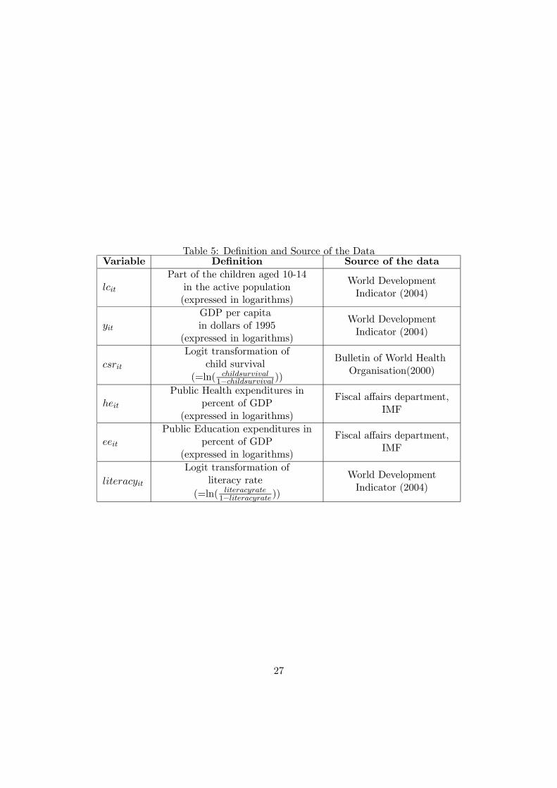
Table 5: Definition and Source of the DataVariable Definition Source of the data

lcit

Part of the children aged 10-14in the active population(expressed in logarithms)

World DevelopmentIndicator (2004)

yit

GDP per capitain dollars of 1995

(expressed in logarithms)


csrit

Logit transformation ofchild survival

(=ln( childsurvival1−childsurvival ))

Bulletin of World HealthOrganisation(2000)

heit

Public Health expenditures inpercent of GDP


Fiscal affairs department,IMF

eeit

Public Education expenditures inpercent of GDP


Fiscal affairs department,IMF

literacyit

Logit transformation ofliteracy rate

(=ln( literacyrate1−literacyrate))


27

0.2 0.4 0.6 0.8 1α

20%

40%

60%

80%

100%

lcHα,TL uH.L=HARA

lcHα,2L

lcHα,15LlcHα,10LlcHα,5L

0.2 0.4 0.6 0.8 1α

20%

40%

lcHα,TL uH.L=LOGlcHα,5L

lcHα,15LlcHα,2L

lcHα,10L

0.2 0.4 0.6 0.8 1α

20%

40%

60%

80%

100%

lcHα,TL uH.L=CRRA

lcHα,15LlcHα,10L

lcHα,2L

lcHα,5L0.2 0.4 0.6 0.8 1

α

20%

40%

60%

80%

100%

lcHα,TL uH.L=CARA

lcHα,10LlcHα,15L

lcHα,2L

lcHα,5L

Figure 2: Optimal level of education investment (γ (α, T )) with the following specifications: δ = 0.6, d = 0.3, w = 30, φ (H) = 1− 11+3H ,

e (E) = 1 +E0.8, U (.) =W (.), and CARA: U (x) = − e−σxσ with σ = 0.014, CRRA: U (x) = x1−R

1−R with R = 0.4, HARA:

U (x) = 1−kA(2−k) (Ax+B)

2−k1−k + C with A = 2, B = 1, k = 3.