Embed Size (px)
Citation preview

8/13/2019 Wholewhole
http://slidepdf.com/reader/full/wholewhole 1/396
DEVELOPMENT AND EVALUATION OF PASSIVE
VARIABLE-PITCH VERTICAL AXIS WIND TURBINES
A thesis submitted for the degree of
Doctor of Philosophy
By
N.C.K. Pawsey
B.E.(Mech)
Supervisor: A.J. Barratt
Co-supervisor: Dr T.J. Barber
School of Mechanical and Manufacturing Engineering,
The University of New South Wales.
November 2002

8/13/2019 Wholewhole
http://slidepdf.com/reader/full/wholewhole 2/396

8/13/2019 Wholewhole
http://slidepdf.com/reader/full/wholewhole 3/396
Abstract
Vertical-axis wind turbines do not need to be oriented to the wind direction and
offer direct rotary output to a ground-level load, making them particularly suit-
able for water pumping, heating, purification and aeration, as well as stand-alone
electricity generation. The use of high-efficiency Darrieus turbines for such applica-
tions is virtually prohibited by their inherent inability to self-start. The provision
of blade-articulation (variable-pitch blades) has been demonstrated by a num-
ber of researchers to make Darrieus turbines self-starting. One aim of this thesis
is to evaluate the various concepts manifested in the numerous specific passive
variable-pitch designs appearing in the literature, often without theoretical anal-
ysis. In the present work, two separate mathematical models have been produced
to predict the performance of passive variable-pitch Darrieus-type turbines. A
blade-element/momentum theory model has been used to investigate the relation-
ships between the key parameter values and turbine steady-state performance. A
strategy for parameter selection has been developed on the basis of these results.
A free vortex wake model for passive variable-pitch turbines has been developed,
allowing the study of unsteady performance. Significant reduction of average ef-
ficiency in a turbulent wind is predicted for a Darrieus turbine. The improved
low-speed torque of passive variable-pitch turbines is predicted to significantly
improve turbulent wind performance.
Two new design concepts for passive variable-pitch turbines are presented that
are intended to allow greater control of blade pitch behaviour and improved tur-
ii

8/13/2019 Wholewhole
http://slidepdf.com/reader/full/wholewhole 4/396
bulent wind performance. A prototype turbine featuring these design concepts
has been designed, constructed and tested in the wind tunnel. As part of this
testing, a technique has been developed for measuring the pitch angle response of
one of the turbine blades in operation. This allows comparison of predicted and
measured pitch histories and gives insight into the performance of turbines of this
type. Results have demonstrated the usefulness of the mathematical models as
design tools and have indicated the potential of one of the new design concepts inparticular to make a vertical axis wind turbine self-starting.
iii

8/13/2019 Wholewhole
http://slidepdf.com/reader/full/wholewhole 5/396
I hereby declare that this submission is my own work and to
the best of my knowledge it contains no materials previously
published or written by another person, nor material which to
a substantial extent has been accepted for the award of any
other degree or diploma at UNSW or any other educational
institution, except where due acknowledgement is made in
the thesis. Any contribution made to the research by others,
with whom I have worked at UNSW or elsewhere, is explicitly
acknowledged in the thesis.
I also declare that the intellectual content of this thesis is the
product of my own work, except to the extent that assistance
from others in the project’s design and conception or in style,
presentation and linguistic expression is acknowledged.
N.C.K. Pawsey
iv

8/13/2019 Wholewhole
http://slidepdf.com/reader/full/wholewhole 6/396
Acknowledgements
I wish to thank all those who have contributed to my work and supported me
during my study. I have been supported by an Australia Postgraduate Award,
while the research was supported by an Australian Research Council Small Grant.
Thank you to my supervisor, Tony Barratt, for introducing me to the field of
wind energy, keeping me on the right track and for getting his hands dirty with
the test rig on numerous occasions.
Thank you to my co-supervisor, Tracie Barber, for her advice, encouragement
and unwavering optimism.
Thank you to the workshop staff who manufactured the prototype turbine com-
ponents and assisted me with the wind tunnel testing, especially Ron Montgomery
and Terry Flynn.
Thank you to Dorothy at Meury Enterprises for her generous donation of glue
and equipment.
Thank you finally to my friends and family who supported me through three
and a half years, and most especially to my beloved Jannet, for whom the struggle
was hardly less arduous, but suffered with good humour and unfailing support.
v
8/13/2019 Wholewhole
http://slidepdf.com/reader/full/wholewhole 7/396
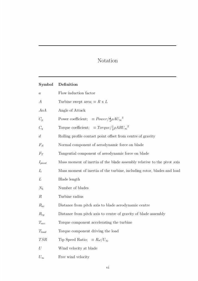
Notation
Symbol Definition
a Flow induction factor
A Turbine swept area; ≡ R x L
AoA Angle of Attack
C p Power coefficient; ≡ Power/ 12ρAU ∞
3
C q Torque coefficient; ≡ Torque/12ρARU ∞
2
d Rolling profile contact point offset from centre of gravity
F N Normal component of aerodynamic force on blade
F T Tangential component of aerodynamic force on blade
I pivot Mass moment of inertia of the blade assembly relative to the pivot axis
I t Mass moment of inertia of the turbine, including rotor, blades and load
L Blade length
N b Number of blades
R Turbine radius
Rac Distance from pitch axis to blade aerodynamic centre
Rcg Distance from pitch axis to centre of gravity of blade assembly
T acc Torque component accelerating the turbine
T load Torque component driving the load
TSR Tip Speed Ratio; ≡ Rω/U ∞
U Wind velocity at blade
U ∞ Free wind velocity
vi

8/13/2019 Wholewhole
http://slidepdf.com/reader/full/wholewhole 8/396
y Rolling profile radial coordinate
y0 Value of rolling profile radial coordinate y at θ = 0
φ Azimuth angle - the orbital position of the blade relative to the wind direction
ρ Air density
θ Blade pitch angle. Positive ‘tail out’
ω Turbine angular velocity
vii

8/13/2019 Wholewhole
http://slidepdf.com/reader/full/wholewhole 9/396

8/13/2019 Wholewhole
http://slidepdf.com/reader/full/wholewhole 10/396
2.2.1 Momentum models . . . . . . . . . . . . . . . . . . . . . . . 39
2.2.2 Vortex models . . . . . . . . . . . . . . . . . . . . . . . . . . 43
2.2.3 Summary . . . . . . . . . . . . . . . . . . . . . . . . . . . . 45
Chapter 3 Design Concepts 47
3.1 Introduction . . . . . . . . . . . . . . . . . . . . . . . . . . . . . . . 47
3.2 Elastomeric Pitch Control Concept . . . . . . . . . . . . . . . . . . 51
3.2.1 Origin of concept . . . . . . . . . . . . . . . . . . . . . . . . 51
3.2.2 Initial geometry testing . . . . . . . . . . . . . . . . . . . . . 53
3.3 Rolling Profile Pitch Control Concept . . . . . . . . . . . . . . . . . 57
3.3.1 Origin of concept . . . . . . . . . . . . . . . . . . . . . . . . 57
3.3.2 Derivation of mathematical basis . . . . . . . . . . . . . . . 57
3.3.3 Application of concept to wind turbines . . . . . . . . . . . 61
3.3.4 Potential advantages . . . . . . . . . . . . . . . . . . . . . . 65
3.4 Experimental Work . . . . . . . . . . . . . . . . . . . . . . . . . . . 74
3.5 Conclusion . . . . . . . . . . . . . . . . . . . . . . . . . . . . . . . . 79
Chapter 4 Development of a Pro/MECHANICA Model 80
4.1 Introduction . . . . . . . . . . . . . . . . . . . . . . . . . . . . . . . 80
4.2 Pro/MECHANICA Model . . . . . . . . . . . . . . . . . . . . . . . 80
4.2.1 Aerodynamic load simulation . . . . . . . . . . . . . . . . . 82
4.3 Summary . . . . . . . . . . . . . . . . . . . . . . . . . . . . . . . . 85
Chapter 5 Momentum Theory Model 86
5.0.1 Background of momentum models . . . . . . . . . . . . . . . 86
5.0.2 Present extension . . . . . . . . . . . . . . . . . . . . . . . . 87
5.0.3 Basis of the mathematical model . . . . . . . . . . . . . . . 88
ix

8/13/2019 Wholewhole
http://slidepdf.com/reader/full/wholewhole 11/396
5.1 Unsteady Aerodynamics including Dynamic Stall . . . . . . . . . . 93
5.1.1 Introduction . . . . . . . . . . . . . . . . . . . . . . . . . . . 93
5.1.2 Attached flow unsteady aerodynamics . . . . . . . . . . . . . 95
5.1.3 Dynamic stall . . . . . . . . . . . . . . . . . . . . . . . . . . 98
5.1.4 Comparisons . . . . . . . . . . . . . . . . . . . . . . . . . . 105
5.1.5 Summary . . . . . . . . . . . . . . . . . . . . . . . . . . . . 106
5.2 Sample Results . . . . . . . . . . . . . . . . . . . . . . . . . . . . . 1075.2.1 Summary . . . . . . . . . . . . . . . . . . . . . . . . . . . . 109
5.3 Limitations of Momentum Theory . . . . . . . . . . . . . . . . . . . 110
5.4 Summary . . . . . . . . . . . . . . . . . . . . . . . . . . . . . . . . 113
Chapter 6 Vortex Theory Model 114
6.1 Background to Vortex Methods . . . . . . . . . . . . . . . . . . . . 114
6.1.1 Reasons for using a free vortex method . . . . . . . . . . . . 114
6.2 Free Vortex Aerodynamic Model . . . . . . . . . . . . . . . . . . . . 116
6.2.1 Treatment of unsteady aerodynamics . . . . . . . . . . . . . 119
6.3 Extension of the Vortex Method for Passive Variable-Pitch VAWTs 122
6.4 Validation Using Published Results . . . . . . . . . . . . . . . . . . 127
6.5 Limitations of Vortex Methods . . . . . . . . . . . . . . . . . . . . . 136
6.6 Motion Simulation Model . . . . . . . . . . . . . . . . . . . . . . . 137
6.7 Constrained Cases . . . . . . . . . . . . . . . . . . . . . . . . . . . 147
6.7.1 Calculation of turbine torque . . . . . . . . . . . . . . . . . 147
6.8 Validation of Motion Simulation Code using Pro/MECHANICA . . 149
6.9 Comparison with Momentum Method . . . . . . . . . . . . . . . . . 150
6. 10 Concl usi on . . . . . . . . . . . . . . . . . . . . . . . . . . . . . . . . 154
x
8/13/2019 Wholewhole
http://slidepdf.com/reader/full/wholewhole 12/396
Chapter 7 Parameter Selection Strategy 155
7.1 Introduction . . . . . . . . . . . . . . . . . . . . . . . . . . . . . . . 155
7.2 Study of Blade Pitch Response Using Pro/MECHANICA . . . . . . 155
7.2.1 Introduction . . . . . . . . . . . . . . . . . . . . . . . . . . . 155
7.2.2 Simulation method . . . . . . . . . . . . . . . . . . . . . . . 156
7.2.3 Results . . . . . . . . . . . . . . . . . . . . . . . . . . . . . . 158
7.2.4 Summary . . . . . . . . . . . . . . . . . . . . . . . . . . . . 1687.3 Parametric Study of an Elastic Passive Pitch System . . . . . . . . 169
7.3.1 Selection of restoring moment parameter . . . . . . . . . . . 169
7.3.2 Selection of aerodynamic moment arm Rac . . . . . . . . . . 179
7.3.3 Blade damping . . . . . . . . . . . . . . . . . . . . . . . . . 183
7.4 Validity of the Spring/Mass/Damper Analogy . . . . . . . . . . . . 187
7.5 Summary . . . . . . . . . . . . . . . . . . . . . . . . . . . . . . . . 190
Chapter 8 Analysis of Turbulent Wind Performance 192
8.1 Introduction . . . . . . . . . . . . . . . . . . . . . . . . . . . . . . . 192
8.2 Performance in a Wind of Varying Velocity . . . . . . . . . . . . . . 192
8.3 Performance in a Wind of Varying Direction . . . . . . . . . . . . . 196
8.4 Performance in “Real” Wind . . . . . . . . . . . . . . . . . . . . . . 200
8.5 Conclusion . . . . . . . . . . . . . . . . . . . . . . . . . . . . . . . . 206
Chapter 9 Experimental Evaluation 209
9.1 Introduction . . . . . . . . . . . . . . . . . . . . . . . . . . . . . . . 209
9.2 Prototype Turbine Design . . . . . . . . . . . . . . . . . . . . . . . 210
9.3 Blade Design . . . . . . . . . . . . . . . . . . . . . . . . . . . . . . 212
9.3.1 Aerodynamic testing of blades . . . . . . . . . . . . . . . . . 221
xi

8/13/2019 Wholewhole
http://slidepdf.com/reader/full/wholewhole 13/396
9.4 Instrumentation . . . . . . . . . . . . . . . . . . . . . . . . . . . . . 225
9.4.1 Torque and speed measurement . . . . . . . . . . . . . . . . 225
9.4.2 Wind speed measurement . . . . . . . . . . . . . . . . . . . 226
9.4.3 Blade pitch measurement . . . . . . . . . . . . . . . . . . . . 227
9.5 Summary . . . . . . . . . . . . . . . . . . . . . . . . . . . . . . . . 247
Chapter 10 Wind Tunnel Test Results 248
10.1 Rig Design Modifications . . . . . . . . . . . . . . . . . . . . . . . . 248
10.1.1 Pivot joint friction . . . . . . . . . . . . . . . . . . . . . . . 248
10.1.2 Brake friction . . . . . . . . . . . . . . . . . . . . . . . . . . 249
10.1.3 Parasitic drag . . . . . . . . . . . . . . . . . . . . . . . . . . 250
10.2 Experimental Procedure . . . . . . . . . . . . . . . . . . . . . . . . 250
1 0 . 3 R e s u l t s . . . . . . . . . . . . . . . . . . . . . . . . . . . . . . . . . . 2 5 1
10.3.1 Fixed blades . . . . . . . . . . . . . . . . . . . . . . . . . . . 251
10.3.2 Type A component . . . . . . . . . . . . . . . . . . . . . . . 251
10.3.3 Type B component . . . . . . . . . . . . . . . . . . . . . . . 252
10.3.4 Type C geometry . . . . . . . . . . . . . . . . . . . . . . . . 267
10.4 Comparison with Theoretical Results . . . . . . . . . . . . . . . . . 269
10.4.1 Type B component . . . . . . . . . . . . . . . . . . . . . . . 271
10.4.2 Type B II geometry . . . . . . . . . . . . . . . . . . . . . . . 276
10.4.3 Type C component . . . . . . . . . . . . . . . . . . . . . . . 287
10. 4. 4 D i scussi on . . . . . . . . . . . . . . . . . . . . . . . . . . . . 290
10. 5 Concl usi on . . . . . . . . . . . . . . . . . . . . . . . . . . . . . . . . 298
10.5.1 Performance of turbine . . . . . . . . . . . . . . . . . . . . . 298
10.5.2 Development of pitch measurement technique . . . . . . . . 299
10.5.3 Performance of mathematical models . . . . . . . . . . . . . 299
xii
8/13/2019 Wholewhole
http://slidepdf.com/reader/full/wholewhole 14/396
Chapter 11 Conclusion 301
11.1 Summary of Research outcomes . . . . . . . . . . . . . . . . . . . . 305
11.2 Conclusion and Recommendations for Further Work . . . . . . . . . 306
References 308
Appendix A Turbine Kinematics 319
A.1 Pendulum Kinematics . . . . . . . . . . . . . . . . . . . . . . . . . 321
A.2 Rolling Profile Kinematics . . . . . . . . . . . . . . . . . . . . . . . 325
A.3 Kinematics of the Kirke-Lazuaskas Design . . . . . . . . . . . . . . 331
A.4 Comparison of Blade Responsiveness for Different Designs . . . . . 335
Appendix B Dynamic Stall Models 337
B.1 Boeing-Vertol (Gormont) Dynamic Stall Model . . . . . . . . . . . 337
B.2 MIT Dynamic Stall Model . . . . . . . . . . . . . . . . . . . . . . . 338
Appendix C Turbine drag 345
Appendix D Aerofoil data 349
Appendix E Code listing 367
Appendix F Photographs of Test Rig 368
xiii

8/13/2019 Wholewhole
http://slidepdf.com/reader/full/wholewhole 15/396
List of Tables
4.1 Key Pro/MECHANICA measures . . . . . . . . . . . . . . . . . . 84
6.1 Turbine parameters for DMS - vortex model comparison . . . . . 151
7.1 Turbine parameters used for DMS study . . . . . . . . . . . . . . 169
8.1 Turbine parameters for variable velocity wind simulation . . . . . 193
8.2 Average power coefficients for the turbine with two different values
of rotor inertia in a wind of sinusoidally varying velocity magnitude.196
8.3 Average power coefficient results for wind of constant velocity
magnitude and sinusoidally varying direction. . . . . . . . . . . . 198
8.4 Turbulence parameters for “real” wind simulation . . . . . . . . . 200
8.5 Parameters of turbines simulated in a “real” wind . . . . . . . . . 203
8.6 Average power coefficient results for five turbines in a turbulent
wind . . . . . . . . . . . . . . . . . . . . . . . . . . . . . . . . . . 208
10.1 Prototype turbine parameters . . . . . . . . . . . . . . . . . . . . 269
xiv

8/13/2019 Wholewhole
http://slidepdf.com/reader/full/wholewhole 16/396
List of Figures
1.1 Growth of installed wind power . . . . . . . . . . . . . . . . . . . 3
1.2 Illustration of Darrieus concept . . . . . . . . . . . . . . . . . . . 7
1.3 Illustration of troposkien Darrieus. . . . . . . . . . . . . . . . . . 8
1.4 Typical variation of angle of attack . . . . . . . . . . . . . . . . . 11
1.5 Typical variation of tangential force . . . . . . . . . . . . . . . . . 12
1.6 Typical variation of torque coefficient with TSR . . . . . . . . . . 13
1.7 Darrieus rotor aerodynamics . . . . . . . . . . . . . . . . . . . . . 17
1.8 Test results of Grylls et al. (1978) . . . . . . . . . . . . . . . . . . 19
1.9 Predicted Cycloturbine performance . . . . . . . . . . . . . . . . . 19
2.1 Darrieus’ cam driven design . . . . . . . . . . . . . . . . . . . . . 24
2.2 Sicard’s patented design . . . . . . . . . . . . . . . . . . . . . . . 26
2.3 Brenneman’s inertial and elastic designs . . . . . . . . . . . . . . . 27
2.4 Leigh’s “automatic blade pitch” design . . . . . . . . . . . . . . . 28
2.5 Sketch of Liljegren’s inertial and spring design (Liljegren, 1984) . . 30
2.6 Images of Sharp’s design included in his patent (1982) . . . . . . . 31
2.7 Patent sketch of Verastegui’s aerodynamic stabiliser design (Ve-
rastegui, 1996) . . . . . . . . . . . . . . . . . . . . . . . . . . . . . 32
2.8 Sketch of the key mechanism of Zheng’s variable pitch stop design
(Zheng, 1984) . . . . . . . . . . . . . . . . . . . . . . . . . . . . . 33
2.9 The ‘pendulum’ type inertial design of Kentfield (1978) . . . . . . 34
2.10 The Kirke-Lazauskas inertial design (Kirke, 1998) . . . . . . . . . 36
xv

8/13/2019 Wholewhole
http://slidepdf.com/reader/full/wholewhole 17/396
3.1 Passive variable-pitch design concepts . . . . . . . . . . . . . . . 50
3.2 The initial elastomeric test piece . . . . . . . . . . . . . . . . . . 54
3.3 Results of testing of initial geometry . . . . . . . . . . . . . . . . 56
3.4 Results of testing of initial geometry in compression only . . . . . 56
3.5 Rolling profile concept . . . . . . . . . . . . . . . . . . . . . . . . 58
3.6 Rolling profile derivation . . . . . . . . . . . . . . . . . . . . . . . 59
3.7 Comparison between rolling profile (a) and pendulum (b) concepts 613.8 Loci of the blade centre of gravity for circular rolling profile . . . . 63
3.9 Use of involute curves to provide tangential constraint for a circu-
lar rolling profile . . . . . . . . . . . . . . . . . . . . . . . . . . . 66
3.10 Calculation of the blade assembly moment of inertia . . . . . . . 67
3.11 Inertial reactions for different designs . . . . . . . . . . . . . . . . 68
3.12 Predicted performance of tailored rolling profile . . . . . . . . . . 70
3.13 Comparison of the d − θ relationships for two ‘linear spring’ profiles 73
3.14 The three second-generation blade mounting part geometries. . . . 75
3.15 Pro/ENGINEER representation of the Type A geometry compo-
nent in place on the prototype turbine. . . . . . . . . . . . . . . . 76
3.16 Test rig for elastomeric blade mounting pieces . . . . . . . . . . . 77
3.17 Results of testing of Type A, B and C geometries. The dashed line
represents the theoretical linearised stiffness for the rolling profile
alone. . . . . . . . . . . . . . . . . . . . . . . . . . . . . . . . . . . 78
4.1 Pro/MECHANICA model of the pendulum type inertial turbine . 81
5.1 Illustration of the Double Multiple Streamtube concept . . . . . . 89
5.2 Iterative procedure used to calculate the flow velocity and blade
motion within a streamtube . . . . . . . . . . . . . . . . . . . . . 91
xvi

8/13/2019 Wholewhole
http://slidepdf.com/reader/full/wholewhole 18/396
5.3 Schematic showing the features of the dynamic stall process . . . 99
5.4 Predicted power coefficient against tip speed ratio showing signif-
icant variation between dynamic stall models. . . . . . . . . . . . 108
5.5 The empirical modification to momentum theory used by Sharpe
(1990) to deal with heavily loaded rotor operation . . . . . . . . . 111
6.1 Discrete vortex representation of the unsteady blade wake . . . . . 117
6.2 Screen capture of the animated output of the free vortex model . . 1236.3 Comparison of predicted blade forces with results of Strickland
et al. (1981), TSR 5 . . . . . . . . . . . . . . . . . . . . . . . . . . 129
6.4 Comparison of predicted blade forces with results of Strickland
et al. (1981), TSR 2.5 . . . . . . . . . . . . . . . . . . . . . . . . 130
6.5 Comparison of predicted blade forces with results of Paraschivoiu
(1983), TSR 3 . . . . . . . . . . . . . . . . . . . . . . . . . . . . . 134
6.6 Comparison of predicted blade forces with results of Paraschivoiu
(1983), TSR 1. 5 . . . . . . . . . . . . . . . . . . . . . . . . . . . . 135
6.7 Schematic of turbine mechanism defining the generalised coordi-
nates q for a turbine of the pendulum type. . . . . . . . . . . . . . 139
6.8 Comparison of Pro/MECHANICA and vortex code predicted pitch
responses for constant wind force . . . . . . . . . . . . . . . . . . 150
6.9 Predicted pitch response for vortex method and Double Multiple
Streamtube (DMS) method. . . . . . . . . . . . . . . . . . . . . . 151
6.10 Predicted torque variation for vortex method and Double Multiple
Streamtube (DMS) method. (a) TSR = 3.1; (b) TSR = 1.0 . . . 153
7.1 Definition of parameters Rac and Rcg. . . . . . . . . . . . . . . . 157
7.2 Pro/MECHANICA steady-state average torque results . . . . . . 158
xvii

8/13/2019 Wholewhole
http://slidepdf.com/reader/full/wholewhole 19/396
7.3 Pro/MECHANICA steady-state pitch responses . . . . . . . . . . 160
7.4 Comparison of the Pro/MECHANICA steady-state pitch and an-
gle of attack patterns for two values of Rac. . . . . . . . . . . . . . 160
7.5 Calculated mass-spring-damper system frequency ratio and phase
angles . . . . . . . . . . . . . . . . . . . . . . . . . . . . . . . . . 161
7.6 Pro/MECHANICA transient pitch responses for two parameter
sets for the constant speed ‘Driver’ case and the variable speed‘Free’ case. . . . . . . . . . . . . . . . . . . . . . . . . . . . . . . 164
7.7 Pro/MECHANICA turbine acceleration fluctuations over two con-
secutive rotor revolutions for two parameter sets. . . . . . . . . . 165
7.8 Pro/MECHANICA turbine shaft reaction force magnitude fluctu-
ations for a locked rotor axis with two different blade inertias. . . 166
7.9 Pro/MECHANICA turbine shaft reaction force magnitude fluctu-
ations for three values of ‘tower’ stiffness. . . . . . . . . . . . . . 167
7.10 Steady-state torque coefficient C q predicted by the momentum
model for a range of TSR and torsion spring constant K . . . . . 170
7.11 Torque coefficient C q predicted by the momentum model for the
three spring characteristics shown in Figure 7.10. For reference
the prediction for a fixed-bladed turbine is also shown. . . . . . . 172
7.12 Pitch response variation with TSR (indicated by colour) for the
three spring characteristics A,B and C shown in Figure 7.10. . . . 173
7.13 Response amplitude and phase angle for harmonic excitation for
a single degree of freedom spring/mass/damper system . . . . . . 176
xviii

8/13/2019 Wholewhole
http://slidepdf.com/reader/full/wholewhole 20/396
7.14 Spring/mass/damper frequency ratio for the three spring charac-
teristics A,B and C. The torque coefficient is shown by colour as
a function of the frequency ratio. . . . . . . . . . . . . . . . . . . 178
7.15 Spring/mass/damper theoretical harmonic excitation response phase
angle for the three spring characteristics A,B and C. . . . . . . . . 179
7.16 Pitch response amplitudes for values of Rac between 25 mm and
200 mm . . . . . . . . . . . . . . . . . . . . . . . . . . . . . . . . 1817.17 Variation in elastic stiffness required to keep the frequency ratio
constant for a range of values of Rac . . . . . . . . . . . . . . . . . 182
7.18 Torque coefficients for a range of values of Rac . . . . . . . . . . . 182
7.19 Comparison of the convergence of predicted torque coefficient Cq
with successive revolutions for different blade damping coefficients. 187
7.20 Stabiliser mass torsion spring analogy . . . . . . . . . . . . . . . . 189
8.1 Variation in power at steady-state in winds of fluctuating magni-
tude for two values of turbine mass moment of inertia . . . . . . . 197
8.2 Fluctuating power transmitted to the load for a wind velocity of
constant magnitude but direction varying sinusoidally between ±45199
8.3 Longitudinal and lateral velocity components generated by the
Dryden turbulence filter. . . . . . . . . . . . . . . . . . . . . . . . 201
8.4 Momentum theory steady-state performance curves for the tur-
bines listed in Table 8.5 . . . . . . . . . . . . . . . . . . . . . . . 204
8.5 Load power generated by four passive variable-pitch turbine sys-
tems and a fixed bladed turbine in a simulated turbulent wind. . 207
8.6 Comparison of the load power generated by the rolling profile tur-
bine with two different rotor inertias . . . . . . . . . . . . . . . . 207
xix

8/13/2019 Wholewhole
http://slidepdf.com/reader/full/wholewhole 21/396
9.1 Turbine in the 3 metre high wind tunnel test section . . . . . . . 211
9.2 Blade design featuring cantilevered counterweights . . . . . . . . . 214
9.3 Detail of blade design concept showing cantilevered counterweight 215
9.4 Finite element mesh . . . . . . . . . . . . . . . . . . . . . . . . . 216
9.5 Colour fringe plot indicating predicted von Mises stress in the
blade skin (a) and the counterweight spar (b) . . . . . . . . . . . 217
9.6 Blade end assembly . . . . . . . . . . . . . . . . . . . . . . . . . . 2199.7 Construction of the blades . . . . . . . . . . . . . . . . . . . . . . 220
9.8 The ‘Type A’ elastomeric blade mounting component on the tur-
bine rig. . . . . . . . . . . . . . . . . . . . . . . . . . . . . . . . . 221
9.9 The author with the finished rig in the wind tunnel. . . . . . . . 222
9.10 Test blade mounted in the wind tunnel . . . . . . . . . . . . . . . 223
9.11 Measured lift and drag coefficients for a test turbine blade . . . . 224
9.12 Variable pitch Darrieus turbine concept showing LED traces. . . . 229
9.13 The target LEDs mounted on one of the blades. . . . . . . . . . . 230
9.14 Two example images of LED traces for blade pitch measurement.
The upper image is for a low tip speed ratio, the lower image for
a high tip speed ratio. . . . . . . . . . . . . . . . . . . . . . . . . 231
9.15 Projection of a circle in the inclined X 2-Y 2 plane onto the image
plane x-y. . . . . . . . . . . . . . . . . . . . . . . . . . . . . . . . 232
9.16 The perspective projection of circles and their bounding squares,
rotated about the X 2 axis, which is parallel to the image plane . . 234
9.17 Elliptical images of concentric circular reference traces. . . . . . . 235
9.18 Geometry of the blade LED trajectories. . . . . . . . . . . . . . . 240
xx

8/13/2019 Wholewhole
http://slidepdf.com/reader/full/wholewhole 22/396
9.19 Illustration of prototype turbine mounted in the 3 metre wind
tunnel test section . . . . . . . . . . . . . . . . . . . . . . . . . . . 242
9.20 Calibration chart obtained by clamping the blade at known angles 243
9.21 Blade pitch measurement results for turbine in operation at ap-
proximately 30 rpm and wind speed 7 m/s . . . . . . . . . . . . . 244
10.1 Type A geometry . . . . . . . . . . . . . . . . . . . . . . . . . . . 251
10.2 Type B geometry . . . . . . . . . . . . . . . . . . . . . . . . . . . 25210.3 Measured torque coefficient versus tip speed ratio for the Type B
purely inertial geometry. . . . . . . . . . . . . . . . . . . . . . . . 253
10.4 Use of the flexible stem to provide ‘cushioned’ pitch limits . . . . 254
10.5 Measured torque coefficient versus tip speed ratio for the Type B
with flexible stem . . . . . . . . . . . . . . . . . . . . . . . . . . . 255
10.6 Torque results for the Type B polyurethane component with flex-
ible stem and upper and lower pivot points. . . . . . . . . . . . . . 256
10.7 Logged speed, torque and wind velocity data for a run of the
Type B inertial/elastic geometry (a). The corresponding power
coefficient curve (b). . . . . . . . . . . . . . . . . . . . . . . . . . 257
10.8 Torque results for the Type B High Density Polyethylene component.258
10.9 Measured blade pitch responses for two blade mounting geome-
tries. . . . . . . . . . . . . . . . . . . . . . . . . . . . . . . . . . 260
10.10 Type B II geometry . . . . . . . . . . . . . . . . . . . . . . . . . . 261
10.11 Torque and pitch results for the Type B II modified geometry. . . 262
10.12 Type B III geometry . . . . . . . . . . . . . . . . . . . . . . . . . 263
10.13 Results for the Type B III geometry. . . . . . . . . . . . . . . . . 264
10.14 Results the Type B III modified geometry with additional spring. 265
xxi

8/13/2019 Wholewhole
http://slidepdf.com/reader/full/wholewhole 23/396
10.15 Type C geometry . . . . . . . . . . . . . . . . . . . . . . . . . . . 267
10.16 Torque coefficient data and measured pitch response for the Type
C geometry . . . . . . . . . . . . . . . . . . . . . . . . . . . . . . 268
10.17 Torque and power coefficient predicted by the Double Multiple
Streamtube (DMS) mathematical model under ideal conditions
(ie no parasitic drag, no blade friction) . . . . . . . . . . . . . . . 270
10.18 Torque coefficient predicted by the Double Multiple Streamtube(DMS) and vortex mathematical models, compared with experi-
mental data . . . . . . . . . . . . . . . . . . . . . . . . . . . . . . 271
10.19 Measured and predicted pitch responses, Type B, TSR 0.3 - 0.7 . 273
10.20 Measured and predicted pitch responses, Type B, TSR 1.1 - 1.6 . 274
10.21 Measured and predicted pitch responses, Type B, TSR 2.1 - 3.0 . 275
10.22 Measured and predicted torque coefficient, Type B II geometry . 277
10.23 Measured and predicted pitch responses, Type B II, TSR 0.3 - 0.7 278
10.24 Measured and predicted pitch responses, Type B II, TSR 0.9 - 1.6 279
10.25 Measured and predicted pitch responses, Type B II, TSR 2.0 - 2.7 280
10.26 Measured pitch responses for the Type B II geometry compared
with predicted pitch responses for Type B II with additional spring;
TSR 0.3 - 0.7 . . . . . . . . . . . . . . . . . . . . . . . . . . . . . 281
10.27 Measured pitch responses for the Type B II geometry compared
with predicted pitch responses for Type B II with additional spring;
TSR 0.9 - 1.6. . . . . . . . . . . . . . . . . . . . . . . . . . . . . 282
10.28 Measured torque coefficient for the Type B II geometry compared
with predicted torque for Type B II with additional spring . . . . 283
xxii
8/13/2019 Wholewhole
http://slidepdf.com/reader/full/wholewhole 24/396
10.29 Measured pitch responses for the Type B geometry compared with
predicted pitch responses for Type B with additional spring; TSR
0.3 - 0.7 . . . . . . . . . . . . . . . . . . . . . . . . . . . . . . . . 284
10.30 Measured pitch responses for the Type B geometry compared with
predicted pitch responses for Type B with additional spring; TSR
1.1 - 1.6. . . . . . . . . . . . . . . . . . . . . . . . . . . . . . . . 285
10.31 Measured pitch responses for the Type B geometry compared withpredicted pitch responses for Type B with additional spring; TSR
2.1 - 3.0. . . . . . . . . . . . . . . . . . . . . . . . . . . . . . . . 286
10.32 Measured torque coefficient for the Type B geometry compared
with predicted torque for Type B with additional spring . . . . . 287
10.33 Measured and predicted torque coefficient, Type C geometry . . . 288
10.34 Measured and predicted pitch responses, Type C, TSR 0.4 - 1.0 . 289
10.35 Measured and predicted pitch responses, Type C, TSR 1.4 - 1.5 . 290
10.36 Comparison of the speed-time histories (a) and corresponding torque
coefficient-TSR curves (b) for the Type C geometry component
with two different initial conditions. . . . . . . . . . . . . . . . . 291
A.1 Kinematics of the blade mass centre . . . . . . . . . . . . . . . . . 320
A.2 Kinematics of the blade mass centre for the ‘pendulum’ type de-
sign . . . . . . . . . . . . . . . . . . . . . . . . . . . . . . . . . . 322
A.3 Kinematics of the rolling profile design concept . . . . . . . . . . 325
A.4 Rolling profile coordinate system, showing the infinitesimal dis-
placements of a point C at (d,y,θ) in terms of infinitesimal changes
in the coordinates. . . . . . . . . . . . . . . . . . . . . . . . . . . 326
xxiii

8/13/2019 Wholewhole
http://slidepdf.com/reader/full/wholewhole 25/396
A.5 Key parameters of the Kirke-Lazauskas design (reproduced from
Kirke, 1998) . . . . . . . . . . . . . . . . . . . . . . . . . . . . . . 332
A.6 Acceleration components of the blade and stabiliser mass for the
Kirke-Lazauskas design (Kirke, 1998) . . . . . . . . . . . . . . . . 333
B.1 Schematic showing the features of the dynamic stall process. Re-
produced from Leishman (2002) . . . . . . . . . . . . . . . . . . . 343
C.1 Measured still air speed decay for five runs. . . . . . . . . . . . . 346C.2 Torque found by numerical differentiation. . . . . . . . . . . . . . 346
D.1 Lift and drag coefficient data from Sheldahl and Klimas (1981)
presented by Lazauskas (2002) . . . . . . . . . . . . . . . . . . . 365
D.2 Lift and drag coefficient data synthesised from experimental data
for angles of attack below 50 and that of Sheldahl and Klimas
(1981) presented by Lazauskas (2002) for higher angles. . . . . . 366
xxiv

8/13/2019 Wholewhole
http://slidepdf.com/reader/full/wholewhole 26/396
Chapter 1
Introduction
1.1 Background
The harnessing of the energy of the wind to perform useful work is a practice that
has been maintained from at least the sixth century until the beginning of the
twenty-first and interest in the field is growing.
Motivation for the increased use of wind-generated power arises from a num-
ber of fronts. Primary among these is the recognised need to reduce Greenhouse
gas emissions in order to avoid catastrophic climate change. While global fossil
fuel supplies remain plentiful, many nations are also wary of reliance on imported
energy sources in an international climate of uncertainty. Wind is an ideal alter-
native to fossil fuels in these regards, as a renewable, non-polluting, local resource.
These are the motivations that are prompting developed nations to increase the
proportion of their energy needs provided by wind energy.
For developing nations, the motivations are different. While the adoption of
large-scale wind electricity generation in the world’s most rapidly growing pop-
ulations would significantly assist the global effort to avert climate change and
improve local pollution problems, it is the decentralised nature of wind that offers
the greatest hope of improvement to a large number of people’s lives. Two billion
people throughout the world have no access to electricity (IEA, 1999). Renew-
able energy including wind is able to provide energy to remote communities and
1

8/13/2019 Wholewhole
http://slidepdf.com/reader/full/wholewhole 27/396
CHAPTER 1. INTRODUCTION 2
in developing nations where no electricity grid exists. In many instances, they
represent the only economically viable means of providing an energy source to
remote areas. The same argument applies to remote communities in countries like
Australia, where vast distances make the extension of the grid uneconomic.
Therefore while the utility-scale electricity-generating horizontal axis wind tur-
bines that are proliferating throughout Europe, the US and Australia are the
current focus of attention, the development of smaller turbines for stand-aloneapplications deserves equal effort. It will be argued that vertical axis wind tur-
bines, if they can be made self-starting while retaining simplicity, could play an
important part in the provision of energy to people without access to grid power.
1.2 Wind Energy Industry
1.2.1 History and current industry status
Utility scale wind turbines
Wind energy’s contribution to global energy supply is currently very small. Ac-
cording to the IEA (2001a), renewable energy sources excluding hydro, combustible
renewables and waste contributed just 0.5% of the global total primary energy sup-
plies in 1999. This category includes wind energy, geothermal, solar and others.
The contribution of this same category to global electricity production was 1.6%
in 1999. Wind energy’s contribution to total US electricity generation was 0.12%
in 1999, constituting some 1% of the renewables category (EERE, 2001). In Aus-
tralia, as of 2001, approximately 9% of electricity supply came from renewables,
the vast bulk of which came from hydro. Only 0.04% of total electricity generation
came from the 41 MW of wind capacity installed in June 2000 (IEA, 2001b).
However global installed wind capacity is increasing rapidly. Figure 1.1 illus-

8/13/2019 Wholewhole
http://slidepdf.com/reader/full/wholewhole 28/396
CHAPTER 1. INTRODUCTION 3
Figure 1: Wind Power Cumulative Capacity
0
5000
10000
15000
20000
25000
30000
European Union 4 39 6 2 9 8 4 4 1 21 1 1 6 8 3 2 51 5 3 46 9 4 77 2 6 4 5 8 9 6 45 1 2 82 2 1 73 19
World 1743 1983 2321 2801 3531 4821 6104 7636 1015313932 1844924000
1990 1991 1992 1993 1994 1995 1996 1997 1998 1999 2000 2001
Source: BTM Consult and EWEA
Figure 1.1: Growth of installed wind power capacity in EU and the world to end 2001(EWEA, 2002)
trates the global and European growth in installed wind generating capacity. At
the end of 2001 the European Union had 17,319 MW of installed wind capacity
(IEA, 2001a), the US 4,258 MW (AWEA, 2002a) and the world total was 24,000
MW (IEA, 2001a). In Europe 4,500 MW of new capacity was installed in 2001,
the most ever in a single year (EIA, 2002). The average annual market growth
rate in Europe over the period 1993 - 2000 was 40% (EWEA, 2002). Towards
the end of this period, the annual capacity installation rate was increasing at 35%
p.a. In the US, 1,700 MW or US$1.7 billion worth of new generating equipment
was installed in 16 states in 2001. This is more than twice the previous record for
installation in one year (732 MW in 1999) (AWEA, 2002b). The more than 6,000
MW of capacity installed globally in 2001 amounts to annual sales of about US$
7 billion (AWEA, 2001).
In Australia, the installed capacity at the end of 2001 had risen to 73 MW, up
128% on the previous year. A further 100 MW is expected to be operational by

8/13/2019 Wholewhole
http://slidepdf.com/reader/full/wholewhole 29/396
CHAPTER 1. INTRODUCTION 4
the end of 2002 (EIA, 2002) and 500 MW of wind projects currently at various
stages of planning and development. This trend is expected to continue.
The European Wind Energy Association (EWEA) has set a target that by 2010
Europe will have 60 GW of installed wind capacity, contributing 4.4% of Europe’s
total electricity generation, up from 1.0% in 2000 (EWEA, 2000). At the start of
2002, 50% of the EU’s wind capacity was in Germany providing some 3.5% of that
country’s electricity. The German government has announced plans to boost thatfigure to “at least 25% by 2025” (EWEA, 2002).
In the US, according to the AWEA, “Wind is well on its way to providing six
percent of our nation’s electricity–as much as 25 million households use annually–
by the year 2020” (AWEA, 2002b).
The Australian Wind Energy Association (AusWEA) has set a target of 5000
MW of installed capacity in Australia by 2010 (IEA, 2001b).
Small wind turbines
Utility-scale wind turbines have a typical generating capacity of hundreds of kilo-
watts to more than a megawatt. However, small turbines ranging from 1 kilowatt
to a few tens of kilowatts find application in non-grid connected, or stand-alone,
roles. Opportunities for wind energy in the field of Remote Area Power Supply are
growing. The Australian Greenhouse Office (AGO, 2002) estimates that there are
in excess of 10,000 stand-alone and hybrid Remote Area Power Supply systems in
Australia. Diesel generators currently provide the bulk of non-grid connected elec-
tricity in regional Australia. High transport costs and the need to reduce Green-
house gas emissions provide a strong motivation to replace diesel with a clean
renewable source of energy such as solar or wind or both. The Australian govern-
ment has launched the Renewable Remote Power Generation Program (RRPGP)

8/13/2019 Wholewhole
http://slidepdf.com/reader/full/wholewhole 30/396
CHAPTER 1. INTRODUCTION 5
to support the replacement of diesel as fuel for off-grid generation by renewable
sources such as wind. RRPGP offers up to 50% rebate of capital cost of new
renewable energy RAPS installations.
1.3 Vertical Axis Wind Turbines (VAWTs)
1.3.1 History
The earliest known wind turbines featured a vertical axis. The earliest known
design was a panemone used in Persia between 500-900 A.D., which had a shield
to block the wind from the half of the rotor moving upwind. It was used to grind
grain and to pump water. It is widely believed that vertical axis windmills have
existed in China for 2000 years, however the earliest actual documentation of a
Chinese windmill was in 1219 A.D. by the Chinese statesman Yehlu Chhu-Tshai
(Dodge, 2001).
A patent for the particular design concept being studied here was filed in France
by military engineer Georges Jean Marie Darrieus in 1925. His idea received lit-
tle attention and in the late 1960s the design was independently re-invented by
Canadian researchers (South and Rangi, 1973) at the National Research Council
in Ottawa. Upon discovering the existing patent, they named the design after
the original inventor. Following the 1973 Arab oil embargo, the Canadians shared
their information with the US Department of Energy, which began a research pro-
gram to develop the technology (Sandia National Laboratories, 1987). Promising
results from a number of test turbines led to two companies - VAWTPOWER and
FloWind - to commence manufacture in the 1980s in California and by the mid
80s, some 500 VAWTs were generating electricity in that state.

8/13/2019 Wholewhole
http://slidepdf.com/reader/full/wholewhole 31/396

8/13/2019 Wholewhole
http://slidepdf.com/reader/full/wholewhole 32/396
CHAPTER 1. INTRODUCTION 7
their blades are travelling sufficiently fast relative to the free-stream flow. Such
turbines operate at TSRs up to approximately 6 and achieve greater efficiencies
than drag turbines. Theoretically achievable peak outputs are comparable to those
obtainable by a horizontal axis wind turbine (HAWT) with the same rotor area.
1.3.3 Explanation of Darrieus concept
y
xφ
αW
V
U
LIFT
DRAG
U FREE WIND
AZIMUTH
270o
0o
90o
Figure 1.2: Illustration of Darrieus concept
Consider the two-dimensional case of a blade moving in a circular path, as
shown in Figure 1.2. As the blade rotates, it experiences a changing relative flow,
which is the vector sum of the local wind speed and the blade’s own speed. Both
the angle of incidence of this relative flow and the magnitude of its velocity vary
with the orbital position of the blade, called the azimuth. In general, the relative
flow always comes from the upwind side of the blade: that is the outer side of the

8/13/2019 Wholewhole
http://slidepdf.com/reader/full/wholewhole 33/396
CHAPTER 1. INTRODUCTION 8
blade on the upwind pass and the inner side on the downwind pass. Thus the angle
of attack swings through positive and negative values each revolution. At small
non-zero angles of attack the lift force generated by the blade has a tangential
component in the direction of rotation. Provided that drag is small, the blade
then contributes positive torque to the rotor on which it is mounted. This torque
is used to drive a load, thus extracting energy from the wind. In the absence of a
free wind the angle of attack is at all times zero and no lift is produced.
Figure 1.3: Illustration of troposkien Darrieus.
Due to the oscillating angle of attack, unlike a HAWT, the blades of the Dar-
rieus turbine always produce a fluctuating force, even in steady conditions. The
original form of the turbine features curved blades that have the shape that a rope
takes when its ends are fixed to a vertical axis and spun, called a troposkien (see
Figure 1.3). This shape is designed to eliminate bending loads in the blade due to
centrifugal force, so that loads are purely tensile. Straight-bladed turbines must
withstand greater bending due to centrifugal loads, but have all of the blade length
operating at the full tip radius and normal to the plane of rotation.

8/13/2019 Wholewhole
http://slidepdf.com/reader/full/wholewhole 34/396
CHAPTER 1. INTRODUCTION 9
1.3.4 Advantages of the vertical axis format
Wilson and Lissaman (1974) state that the Darrieus rotor has performance near
that of a propeller-type rotor. The principal advantages of the vertical axis format
are the ability to accept wind from any direction without yawing and the ability
to provide direct rotary drive to a fixed load.
The absence of yaw requirement simplifies the design of the turbine. Hansen
et al. (1990) state that failures of yaw drive subsystems have been the second
leading cause of horizontal axis turbine downtime in California. They state also
that smaller turbines with free-yaw (passive) systems also experience problems,
such as overloading due to excessive yaw rates and poor alignment with the wind.
The vertical turbine axis allows rotary loads to be driven directly. For example,
a generator may be driven either at the top of the tower or at ground level without
the need to mount it within the yawing nacelle. Wiring to the generator may be
fixed, rather than having to pass through slip rings and without requiring some
periodic ‘untwisting’ mechanism. A rotary drive pump, such as a helical rotor
borehole pump, may be driven directly, or using a step up belt drive at ground
level. There is anecdotal evidence of attempts to connect horizontal axis wind
turbines to such loads using bevel gearing resulting in the turbine being yawed
away from the wind by the shaft reaction torque.
VAWTs are also well suited to other, low speed, vertical axis loads such as the
aeration and destratification of ponds and the heating of water or other working
fluid by direct mechanical agitation.
A further potential application is the desalination or purification of water by re-
verse osmosis, for which the pressure head can be maintained by direct mechanical
input, bypassing the mechanical-electrical-mechanical conversion step.

8/13/2019 Wholewhole
http://slidepdf.com/reader/full/wholewhole 35/396
CHAPTER 1. INTRODUCTION 10
The market niche for vertical axis wind turbines is in relatively small-scale
applications such as these, and in Remote Area Power Supply uses in general.
To realise the potential of the format however, Darrieus turbines must be made
reliably self-starting without sacrificing mechanical simplicity.
1.4 Low and Intermediate Tip Speed Ratio Performance
Darrieus turbine blades typically use aerofoil sections designed as aircraft wing
profiles. The NACA0012, NACA0015 and NACA0018 profiles are commonly used
as blade sections. Typically these are designed to operate at small angles of attack
(less than 10). At angles higher than this the aerofoil undergoes stall: the flow
separates from the upper surface of the wing causing a loss of lift and an increase
in drag.
As explained in Section 1.3.3, each blade experiences a periodically varyingvelocity and angle of incidence of apparent flow. The amplitude of this variation is
related to the tip speed ratio. This is illustrated in Figure 1.4. This is a simplified
representation of the change in angle of attack pattern with TSR. For simplicity
the effect of the turbine on the free wind velocity is neglected. In reality, as
turbine speed increases, more energy is extracted from the stream and the flow
is decelerated. This causes the ‘effective TSR’ felt by the blade to be greater
than is assumed here. However the relationship is qualitatively similar. At start
up, the angle of attack varies right through 360. At TSR 1, the angle of attack
ranges from -180 to +180. For TSR > 1, the cyclical variation in angle of attack
approaches a sinusoid of decreasing amplitude. As the blade’s velocity becomes
much larger than the free wind velocity, the amplitude of the variation approaches
zero.

8/13/2019 Wholewhole
http://slidepdf.com/reader/full/wholewhole 36/396

8/13/2019 Wholewhole
http://slidepdf.com/reader/full/wholewhole 37/396

8/13/2019 Wholewhole
http://slidepdf.com/reader/full/wholewhole 38/396
CHAPTER 1. INTRODUCTION 13
not stall at any point in the revolution. There are then two distinct peaks in
thrust separated by valleys where tangential force is zero or slightly negative,
corresponding to the points when the angle of attack passes through zero.
It should be remembered that in this simplified analysis the deceleration of
the flow is neglected and in reality the TSR at which stall is eliminated will in
general be lower than is shown here. The trends illustrated however remain valid
and explain the low torque produced by fixed bladed Darrieus turbines at low andintermediate TSRs. Figure 1.5 shows the variation in tangential force for a single
blade. For a turbine with three blades the total torque is smoother, being the
summation of three such curves with 120 phase separation. The average turbine
torque for a revolution is found by integration of this tangential load. This is
shown in Figure 1.6.
-0.1
0
0.1
0.2
0.3
0.4
0.5
0.6
0.7
0.8
0 1 2 3 4 5 6 7 8 9 10
TSR
C q
Figure 1.6: Illustration of the variation of non-dimensionalised torque C q with TSR forthe case shown in Figure 1.5. Because deceleration of the wind is neglected the torque
rises later, achieves a higher peak and persists to higher TSRs than would occur inreality.

8/13/2019 Wholewhole
http://slidepdf.com/reader/full/wholewhole 39/396
CHAPTER 1. INTRODUCTION 14
Figure 1.6 illustrates the trough in the torque curve that occurs at intermediate
tip speed ratios - between approximately 0.5 and 2.5 here. At TSR < 0.5 torque
is slightly positive due to the difference in drag between advancing and retreating
halves of the each blade’s revolution. Thus the turbine may well begin to move
from rest and accelerate up to some equilibrium speed at TSR ≈ 0.5. However
the trough where torque is negative prevents the turbine from accelerating of its
own accord to the TSR at which torque increases rapidly (and above which usefulwork can be done).
The addition of flow deceleration, parasitic aerodynamic drag, transmission
friction and load torque to this simplified analysis would serve only to exacerbate
the inability to self-start. The only real factor neglected here that would improve
starting performance is the consideration of unsteady aerodynamic effects. Under
dynamic conditions, the flow is able to remain attached and stall is delayed to
higher angles of attack than apply under static conditions. These effects are im-
portant to the analysis of Darrieus starting performance and are also very difficult
to accurately account for. This subject will be discussed in detail in Chapter 5.
The actual location and depth of the torque trough is dependent on a number
of factors, including the number and size of the blades, the radius of the turbine
and the free wind velocity. In some cases the torque in the trough may actually
be small but positive. The most serious consequence of this characteristic is the
inability to reliably self-start. While the turbine may be able to begin spinning
and accelerate up to a speed where the torque curve reaches zero, it is not able
to accelerate beyond the trough to the high TSRs at which torque is high enough
for useful work to be done. Even if the ideal torque curve is at all speeds positive,

8/13/2019 Wholewhole
http://slidepdf.com/reader/full/wholewhole 40/396
CHAPTER 1. INTRODUCTION 15
parasitic aerodynamic drag, drive train friction and load resistance are likely to
exceed output torque in the trough.
The inability to self-start is not a major impediment to large grid-connected
turbines with control mechanisms that are able to drive the turbines up to speed
when sufficient wind is measured. However it is a virtually prohibitive shortcoming
for small, stand-alone turbines, which need to operate passively and unattended,
to be economically viable.The negative torque region that prevents self-starting in a steady wind presents
a further problem for turbines operating in turbulent wind. In a real wind, ve-
locity fluctuations occur very much faster than inertia allows the turbine speed to
respond. Thus the instantaneous tip speed ratio varies significantly. If the torque-
speed curve has a deep trough immediately below the running TSR range, there
will be frequent periods during which the torque is low or negative. This may sig-
nificantly affect the total energy captured from the wind. As pointed out by Bayly
(1981), this phenomenon is especially significant for turbines driving synchronous
generators that are made to operate at a constant speed.
The primary focus of this thesis therefore is the investigation of methods of
increasing the torque produced by Darrieus turbines at intermediate tip speed
ratios, so that they may be reliably self-starting and more efficient in turbulent
wind conditions.
1.5 Variable-Pitch Darrieus Turbines
A number of methods for making a Darrieus turbine self-starting have been pro-
posed by previous researchers. A review of these is given by Kirke (1998). The
particular method studied here is the variable-pitch turbine design. It appears to

8/13/2019 Wholewhole
http://slidepdf.com/reader/full/wholewhole 41/396
CHAPTER 1. INTRODUCTION 16
offer the greatest potential for achieving significantly increased torque at low and
intermediate tip speed ratios without compromising peak efficiency.
As discussed in Section 1.4, the inability to self-start is due to the stalling of
the blades at low and intermediate tip speed ratios. Stall occurs when the angle
of attack becomes too large and the flow separates from the surface of the blade
resulting in a loss of lift and an increase in drag. If the angle of attack can be
reduced sufficiently, the flow over the blade can remain attached. This reductionin angle of attack requires that the blade orientation be changed to point closer
to the apparent wind direction. Figure 1.4 shows that if the blade pitch angle is
varied as an approximately sinusoidal function of the azimuth angle, in phase with
the variation in angle of attack, the amplitude of the angle of attack oscillation
experienced by the blade can be reduced. Any reduction in the proportion of time
that the blade spends stalled will increase the average torque for the revolution.
Reduction of stall is the principal mechanism by which variable-pitch increases
torque at intermediate TSRs, but the concept may also produce significant im-
provements at start up and low TSRs. Below TSR = 1, it is not practical for
a blade to pitch sufficiently quickly to prevent stall. However even for moderate
pitch amplitudes, the blades are able to act as more efficient drag devices, like
the mainsail of a yacht running before the wind with the boom swung wide from
the keel line. These two separate mechanisms are able to significantly increase
the starting and intermediate TSR performance of Darrieus turbines. They are
illustrated in Figure 1.7.
1.5.1 Active variable-pitch
The question then is how to produce the required variation in blade pitch. A
central cam with pushrods connected to the blades may be used to produce a

8/13/2019 Wholewhole
http://slidepdf.com/reader/full/wholewhole 42/396
CHAPTER 1. INTRODUCTION 17
LOW TSR
INTERMEDIATE TSR
HIGH TSR
α
W
V
U
LIFT
DRAG
αW
V
U
LIFT
DRAG
α
W
V
U
LIFT
DRAG
αW
V
U
LIFT
DRAG
FIXED PITCH VARIABLE PITCH
α
W
V
U
LIFT
DRAG
α
W
V
U
LIFT
DRAG
Figure 1.7: Darrieus rotor aerodynamics. Blade pitch variation allows the angle of attack to be reduced. At high TSR, no pitching is required. At intermediate TSR,
pitching prevents the blade stalling. At low TSR, pitching produces a more favourablecombination of lift and drag.

8/13/2019 Wholewhole
http://slidepdf.com/reader/full/wholewhole 43/396
CHAPTER 1. INTRODUCTION 18
periodic variation in pitch angle as a function of azimuth angle. Such designs have
been tested by a number of researchers, including Drees (1978) and Grylls et al.
(1978). It is clear from Figure 1.4 that as the amplitude of the angle of attack
variation on a fixed blade decreases with tip speed ratio, so does the amplitude of
pitch variation required to prevent or reduce stalling.
This was confirmed experimentally by Grylls et al. (1978), whose results are
shown in Figure 1.8. They tested a variable-pitch VAWT whose blades were drivenby a central cam. They tested four different amplitudes of pitch variation and
found that while a large amplitude offered good starting torque and low TSR
performance, the turbine was unable to accelerate to higher TSRs, or to produce
a good maximum efficiency. Conversely, a small pitch amplitude was found to
produce good high speed efficiency, but the low TSR benefits were lost.
This finding was confirmed by mathematical modelling of a cam-driven turbine
by Pawsey and Barratt (1999). To elaborate on these results, a series of simula-
tions was run using the momentum theory mathematical model developed for this
project and discussed in Chapter 5. The performance of a turbine with a preset
sinusoidal pattern of pitch variation was predicted at a wind speed of 7 m/s for
different pitch amplitudes, ranging from ±30 to fixed blades. The dimensions and
solidity of the turbine are the same as those tested by Grylls et al.
The results for gross power coefficient C p (parasitic drag not subtracted) are
shown in Figure 1.9. The requirement for pitch amplitude to diminish with TSR is
confirmed. In this case, the predicted gross power is positive at all TSRs, even for
the fixed-blade turbine (0 amplitude). However a significant improvement in low
and intermediate TSR performance is indicated given the appropriate pitch am-
plitude. These results indicate the desirability of having a pitch variation schedule

8/13/2019 Wholewhole
http://slidepdf.com/reader/full/wholewhole 44/396
CHAPTER 1. INTRODUCTION 19
Figure 1.8: Power coefficient wind tunnel test data from Grylls et al. (1978) for a 2.4metre diameter x 1.6 metre VAWT with a cam-driven blade pitch schedule
0
0.05
0.1
0.15
0.2
0.25
0.3
0.35
0.4
0.45
0 1 2 3 4 5 6
TSR
C p
30o
25o
20o
15o
12o
10o
8o
6o
2o
4o
0o
18o
Diameter 2.4 m x height 1.6 m
3 NACA 0018 blades
Chord 145 mm
Figure 1.9: Predicted performance of a cam-driven variable pitch VAWT for a range of
pitch amplitudes. Gross power coefficient is shown, before parasitic drag and frictionare subtracted. Turbine 2.4 metre diameter x 1.6 metre, 3 blades NACA 0018, chord145 mm.

8/13/2019 Wholewhole
http://slidepdf.com/reader/full/wholewhole 45/396
CHAPTER 1. INTRODUCTION 20
whose amplitude is variable. The turbine could then ‘ride the envelope’ of the in-
dividual curves in Figure 1.9, producing improved performance at tip speed ratios
from 0 to the higher design speeds of the standard Darrieus turbine.
This is difficult to achieve in practice with a cam design. Some measurement
and control system would also be required to sense the wind speed relative to the
rotor speed.
This is a major reason for opting for a ‘passive’ variable-pitch system: one inwhich the pitch of the blades is determined directly by the wind forces on the blades
themselves. This removes the need for any sensing or central control and provides
the flexibility needed to overcome the limitations inherent in pre-determining the
blade pitch schedule.
1.5.2 Passive variable-pitch
The basis for the passive variable-pitch concept is that a blade that is free to pitch
about a spanwise (longitudinal) axis near the leading edge will seek to point into
the apparent wind.
Work done by Bayly and Kentfield (1981) and Kirke and Lazauskas (1993)
has demonstrated the ability of two different passive variable-pitch VAWTs to
achieve self-starting. Their work however also demonstrated the sensitivity of the
performance of their turbines to variation in the key parameters that affected the
blade pitch response. While an approximately sinusoidal pattern of pitch variation
is required, the amplitude, phase and higher order deviations from this pattern
have a great effect on the torque at any given speed. Under static conditions,
the magnitude of the equilibrium angle of attack adopted by a blade depends on
the relative strengths of the aerodynamic and restoring moments about the pivot
axis. Under dynamic conditions, the inertia of the blade becomes significant and

8/13/2019 Wholewhole
http://slidepdf.com/reader/full/wholewhole 46/396
CHAPTER 1. INTRODUCTION 21
the combination of these three factors determines the blade pitch response. The
magnitudes of all three of these factors may be determined by the specific design of
the blade and its connection to the rotor. It is the aim of this thesis to investigate
the features of desirable passive blade pitch response and the ways in which such
response may be achieved through the design of the blade-rotor connection.
1.6 Structure of Thesis
Mathematical modelling
In order to evaluate different turbine designs and their performance under differ-
ent operating conditions a mathematical model is required. Bayly and Kentfield
(1981) and Kirke and Lazauskas (1993) developed steady-state performance pre-
diction models for their respective designs. To assess the potential of different
designs for achieving desirable pitch response, for this thesis a more general math-
ematical model has been developed for steady-state performance. In addition, a
separate model has been developed for investigation of transient turbine behaviour,
especially performance in turbulent conditions.
New turbine design
On the basis of insights gained from the results of theoretical analysis, two new
design concepts have been conceived and studied. Predicted performance is pre-
sented for these designs and explanation of their potential advantages is given.
Experimental procedure
In order to assess the potential of the new design concepts, a prototype turbine has
been designed and constructed and tested in a wind tunnel. A new technique for
measuring the blade pitch response pattern of the turbine in operation has been

8/13/2019 Wholewhole
http://slidepdf.com/reader/full/wholewhole 47/396
CHAPTER 1. INTRODUCTION 22
developed. Results of this testing and conclusions on the potential of the designs
are presented.

8/13/2019 Wholewhole
http://slidepdf.com/reader/full/wholewhole 48/396
Chapter 2
Review of Passive Pitch Control Systems for Darrieus
Turbines
2.1 Review of Existing Variable-Pitch Darrieus Turbines
2.1.1 Active variable-pitch Darrieus turbines
Variable-pitch Darrieus turbines may be divided into active and passive types.
Active designs may be defined as those systems that produce blade pitch change
through means other than the direct action of the aerodynamic forces acting on
them. These may range from systems that measure and calculate appropriate pitch
angles continuously and use hydraulic or similar actuators to drive the blades to
the desired angle, through to cam-driven designs mentioned in Section 1.5.
Work has been done on this type of turbine by McConnell (1979) and Meikle
(1993). The cost and complexity of such systems is not considered justifiable for
small stand-alone turbines. A more simple type of active system is one in which
the blades are moved by pushrods driven by a central cam, which produces a pre-
set schedule of pitch variation. Darrieus (1931) included such a cam-driven design
in his original patent for the fixed-pitch turbine (see Figure 2.1). Drees (1978)
developed a similar design called a ’Cycloturbine’ with the Pinson Energy Corpo-
ration. The blade pitch schedule is set using a central cam and pushrods to each
blade. The cam is oriented with the wind direction using a small tail vane. Drees
23

8/13/2019 Wholewhole
http://slidepdf.com/reader/full/wholewhole 49/396
CHAPTER 2. REVIEW OF PASSIVE PITCH SYSTEMS 24
Figure 2.1: Darrieus’ cam driven design
reported reliable self-starting and a high maximum power coefficient Cp of 0.45 in
field tests. As mentioned in Section 1.4, Grylls et al. (1978) performed theoretical
and experimental analysis of a turbine similar to that of Drees. They developed a
multiple streamtube type mathematical model that incorporated a preset schedule
of pitch variation. Both theoretical and wind tunnel results indicated one of the
major problems of such active designs: the amplitude of the pitch variation is fixed
by the cam and so cannot vary to suit the tip speed ratio. This limits the efficient
performance of the turbine to a narrow band of TSR. Large amplitude (±20)
produces good starting torque and performance up to TSR 1.5, which then drops
off rapidly with increasing speed. A small amplitude of ±5 yields good high speed
performance (and much higher efficiency) at the detriment of starting performance.
This limitation could be overcome by providing some means of varying the cam
profile with turbine speed, however the technical difficulty of accomplishing this
would greatly increase the cost.
Grylls et al. also reported problems of high friction associated with the cam
and pushrod mechanism. These problems and the increased cost and complexity

8/13/2019 Wholewhole
http://slidepdf.com/reader/full/wholewhole 50/396
CHAPTER 2. REVIEW OF PASSIVE PITCH SYSTEMS 25
of active systems are the reason for the exclusive focus on passive designs in the
current work.
2.1.2 Passive variable-pitch Darrieus turbines
Sicard (1977) patented a design in which the blades are free to pivot about an axis
in the chord line and are balanced so that their centre of mass lies radially outboard
of the pivot axis when the blade is in a ‘zero-pitch’ position - i.e. with its chord line
tangential to the orbit of the pivot axis. This design is shown in Figure 2.2. Under
the action of centrifugal ‘force’ a stabilising or restoring moment is applied to the
blade so that it seeks the zero-pitch position. Thus the blade is like a pendulum
in an inertial field. No stops are mentioned to limit the pitch angle of the blades
and so at rest there is nothing to prevent the blades all turning to point into the
wind, thus generating no thrust.
Sicard does mention a variation on the design in which the upper ends of the
blades are mounted at a slightly larger radius than the lower ends, thus causing
the blades to seek a zero pitch orientation at rest under the influence of gravity. It
seems unlikely however that for small tilt angles this would produce enough mo-
ment to allow the turbine to self-start using the drag of the blades. No theoretical
or experimental analysis of the design by Sicard was found.
Brenneman (1983) designed a turbine that in one form, which he terms an
‘inertial’ type, is identical to Sicard’s design with the addition of stops to limit
pitch angle. A second embodiment, which he calls an ‘elastic’ type, has the blades
balanced about the pivot axis, with some elastic device, such as a steel rod or
wire spring, to return the blade to its undisturbed position as shown in Figure 2.3.
For this design he makes the claim that it is inherently speed limiting, as the
natural frequency of the blade oscillation is fixed by the moment of inertia of the

8/13/2019 Wholewhole
http://slidepdf.com/reader/full/wholewhole 51/396

8/13/2019 Wholewhole
http://slidepdf.com/reader/full/wholewhole 52/396
CHAPTER 2. REVIEW OF PASSIVE PITCH SYSTEMS 27
a pitch amplitude that increases with speed will result. This is the opposite of the
trend that is desirable, as discussed in Section 1.5.
No experimental work to test the design concept is mentioned. An essentially
identical concept is embodied in the design of Cameron (1978).
Figure 2.3: The elastic (left) and inertial designs of Brenneman (1983)
Leigh (1980) proposed a design in which each blade is pivoted about a point
on the chord forward of the aerodynamic centre. The blade is balanced using
a counterweight hidden inside the radial arm (thus reducing parasitic drag) and
acting on the blade via a pushrod (see Figure 2.4). Springs produce a restoring
moment on the blade, returning it to the neutral position. Like Brenneman’s
elastic design, the restoring moment is independent of the centrifugal load and the
turbine should behave in the same manner as Brenneman’s.
Evans (1978) designed a passive variable pitch turbine in which the blades were
pivoted about a point at the 1/3 chord location and balanced about this point.
The stated aim of the design was to allow the blade to pitch to reduce the angle
of attack so that it is just below stall. The concept is based on pitching moment,

8/13/2019 Wholewhole
http://slidepdf.com/reader/full/wholewhole 53/396
CHAPTER 2. REVIEW OF PASSIVE PITCH SYSTEMS 28
Figure 2.4: Leigh’s ”automatic blade pitch” design concept (reproduced from Leigh,1980)
or movement of the centre of pressure. For angles of attack well below stall, the
centre of pressure should be forward of the pivot axis (near the quarter chord),
while if stalled, the centre of pressure should be aft of the 1/3 chord position.These movements were intended to always move the blade to the angle of attack
that was considered ideal, just below stall. The stated role of the spring is to bias
the pitch in the direction of decreased angle of attack, though it appears that it
would actually reduce the angle of pitch, which would often increase the angle of
attack.
As no test data is given for the turbine, it is difficult to say whether this concept
could be successful. Evans also proposed a design in which the blades are free to

8/13/2019 Wholewhole
http://slidepdf.com/reader/full/wholewhole 54/396

8/13/2019 Wholewhole
http://slidepdf.com/reader/full/wholewhole 55/396
CHAPTER 2. REVIEW OF PASSIVE PITCH SYSTEMS 30
Figure 2.5: Sketch of Liljegren’s inertial and spring design (Liljegren, 1984)

8/13/2019 Wholewhole
http://slidepdf.com/reader/full/wholewhole 56/396

8/13/2019 Wholewhole
http://slidepdf.com/reader/full/wholewhole 57/396
CHAPTER 2. REVIEW OF PASSIVE PITCH SYSTEMS 32
Figure 2.7: Patent sketch of Verastegui’s aerodynamic stabiliser design (Verastegui,1996)
The exact theory by which this is achieved is not disclosed, though a momen-
tum type analysis included in the patent is used to derive predictions of peak
power coefficient of 0.70 for the design, which exceeds the Betz limit for maximum
theoretical C p of 0.593.
In addition to his work on the Cycloturbine described above, Drees (1979)
also patented a passive variable-pitch turbine in which the blades are not bal-
anced about their pivot point. In the simplest form of the invention, the blades
are allowed to swing inwards through 90 to act as drag translators at very low
tip speed ratios. As speed increases, centrifugal force holds the blades out in a
zero-pitch position against stops. Thus the design seeks to make use only of the
start up drag-dominant mode and the lift-dominant running mode of the standard

8/13/2019 Wholewhole
http://slidepdf.com/reader/full/wholewhole 58/396
CHAPTER 2. REVIEW OF PASSIVE PITCH SYSTEMS 33
Darrieus turbine, without any means of extending the lift-based operation down
to intermediate tip speed ratios. As such is seems unlikely to achieve self-starting.
Zheng (1984) recognised the need to have a progressively diminishing ampli-
tude of pitch response with increasing turbine speed for a given wind speed. His
design has no means of providing a restoring moment on the blade to balance aero-
dynamic moments, but instead features a weighted ‘guide’ piece that progressively
narrows the angle through which the blade is allowed to swing (see Figure 2.8).It is not clear whether this design concept could work, however from a practical
standpoint the repeated impact of the swinging blade on the hard stops is likely
to be problematic.
Figure 2.8: Sketch of the key mechanism of Zheng’s variable pitch stop design (Zheng,1984)

8/13/2019 Wholewhole
http://slidepdf.com/reader/full/wholewhole 59/396
CHAPTER 2. REVIEW OF PASSIVE PITCH SYSTEMS 34
Martin (1989) patented a turbine in which cambered blades are free to pivot
about a point near the leading edge and are balanced using a counterweight about
a point on the chord line but forward of the pivot axis.
Bayly and Kentfield (Bayly, 1981; Bayly and Kentfield, 1981) performed a theo-
retical and experimental study on a turbine design they called a “Cyclobrid”. This
was a passive-pitching turbine essentially identical in concept to that patented by
Sicard (1977), but apparently conceived independently by Kentfield (1978). Kent-field however used stops to limit the travel of the blades, thus allowing the turbine
to start from rest (see Figure 2.9). Bayly produced a momentum type mathemat-
Figure 2.9: The ‘pendulum’ type inertial design of Kentfield (1978)

8/13/2019 Wholewhole
http://slidepdf.com/reader/full/wholewhole 60/396
CHAPTER 2. REVIEW OF PASSIVE PITCH SYSTEMS 35
ical model for the turbine and tested a 15 foot (4.57 m) diameter prototype. The
mathematical model indicated good running efficiency for the design.
The full-scale prototype turbine tested in the field achieved reliable self-starting
and a peak efficiency of 0.36 at a tip speed ratio of 3.7, which are in reasonable
agreement with predictions of the mathematical model. This work demonstrated
the ability of the passive variable-pitch systems to marry self-starting ability with
good running speed efficiency. It also demonstrated the ability of an inertial typepitch control system to produce appropriate pitch response over a range of turbine
speeds.
Kirke (1998) conducted a study on self-starting vertical axis wind turbines as
a PhD thesis. Kirke performed an extensive survey of previous active and passive
variable pitch VAWT designs and his thesis is the most detailed and systematic
work on passive variable-pitch turbines found in the literature. He considered
passive variable-pitch Darrieus type turbines as just one of a number of options
available for achieving self-starting, but devoted most of his attention to them and
in particular the design he developed with Lazauskas (Kirke and Lazauskas, 1991).
The design concept is shown in Figure 2.10.
Kirke’s design is very similar in concept to that of Liljegren (1984), though
much simpler in execution. A single T-shaped stabiliser mass is used to oppose
the pitching of the blade, which is balanced about a point on the chord line near
the leading edge. No springs are used to assist the masses at low speeds in this case.
This design produces a restoring moment that is proportional to the centrifugal
force but is independent of the pitch angle.
Unlike Liljegren’s design, Kirke provided the ability to adjust the moment
arms at which the two masses acted independently, as well as the respective pitch

8/13/2019 Wholewhole
http://slidepdf.com/reader/full/wholewhole 61/396
CHAPTER 2. REVIEW OF PASSIVE PITCH SYSTEMS 36
Figure 2.10: The Kirke-Lazauskas inertial design (Kirke, 1998)
limits. This allows the pitch response to be biased in one direction or the other.
Unlike the ‘pendulum’ type of inertial system tested by Bayly and Kentfield (1981),
Kirke’s design has a threshold of restoring moment that must be exceeded by the
aerodynamic moment on the blade before any pitching will occur. This feature
is desirable because it prevents small oscillations at high speeds that occur with
pendulum type designs and allows the turbine to function as a standard fixed-
blade Darrieus turbine at high running speeds. However at lower TSR when the
pitch response amplitude is large there will be an impact between the blade and
the stabiliser mass each time the blade swings through the zero pitch position, as
the mass switches contact points and is asked to change direction instantaneously.
Thus the contact points between blade and mass would need to be cushioned in
some way to avoid damaging impact loading and prevent ‘bouncing’ in the pitch
response.

8/13/2019 Wholewhole
http://slidepdf.com/reader/full/wholewhole 62/396
CHAPTER 2. REVIEW OF PASSIVE PITCH SYSTEMS 37
It should also be noted that compared with the Kentfield ‘pendulum’ type
design, Kirke’s separation of the pivoting blade and the sliding stabiliser mass
does not necessarily result in a reduced moment of inertia of the blade or faster
pitch response. The radial movement of the stabiliser mass associated with blade
pitching adds to the effective mass moment of inertia about the pivot axis. It can
be shown that this effect is equivalent to lumping the stabiliser mass at the contact
point. This additional inertia was not included in the mathematical model (Kirkeand Lazauskas, 1992).
The model was of the momentum type and was validated through wind tunnel
testing of a model turbine. He also built and tested in the field a 6 metre diameter
turbine based on the same design. Some discrepancy was found between predicted
and measured results for this case. Both the wind tunnel and field testing demon-
strated the ability of the design to achieve self-starting and his results lend further
weight to the argument for inertial type pitch control.
2.1.3 Summary
From the wide range of often ingenious ideas embodied in the above designs a num-
ber of common themes emerge. By definition, all passive variable-pitch turbines
rely on aerodynamic forces to effect the change in blade pitch.
Drees and Evans produced designs in which the blades are not independent,
but instead move collectively. Martin, Drees and Zheng produced designs that rely
purely on aerodynamic forces to move the blades. While centrifugal force is used
to limit or prevent pitching at high speeds, it does not continuously influence the
pitch response.
All the remaining passive designs regulate the pitch response using a restoring
moment on the blades that counteracts the tendency of the wind to disturb the

8/13/2019 Wholewhole
http://slidepdf.com/reader/full/wholewhole 63/396
CHAPTER 2. REVIEW OF PASSIVE PITCH SYSTEMS 38
blade from its neutral position. Brenneman and Cameron produced designs in
which the restoring moment is provided by purely elastic means. Sharp, Sicard,
Kentfield and Kirke relied on inertial forces in their designs. Brenneman and
Liljegren also produced designs that used a combination of the two.
While Brenneman talks about elastic and inertial means of pitch control as
being different means of producing essentially the same effect, the major difference
between them is that the restoring moment provided by the elastic means (asembodied to date) is independent of the turbine speed. Inertial loads on the other
hand are inherently proportional to the square of the turbine speed. The only
designs demonstrated to be effective to date (Bayly and Kentfield, 1981; Kirke
and Lazauskas, 1993) have utilised inertial pitch control. It will be shown that
such a relationship should be the starting point for effective pitch control, though
deviations from it may be required to optimise performance over the entire speed
range.
The number and variety of the designs described above indicates the need for a
systematic approach to the treatment of the problem of self-starting. Most of the
above designs appear with minimal theoretical basis presented in the patent and
no supporting work appearing in the literature. The aerodynamics and dynamics
of passive variable-pitch mechanisms are too complex to be effectively handled
without detailed quantitative analysis. The development of mathematical tools to
predict what is desirable pitching behaviour and what designs might go closest to
realising this is the primary aim of the present work.

8/13/2019 Wholewhole
http://slidepdf.com/reader/full/wholewhole 64/396
CHAPTER 2. REVIEW OF PASSIVE PITCH SYSTEMS 39
2.2 Review of Mathematical Models for Variable-Pitch Darrieus
Turbines
The two most studied and best validated approaches to the mathematical mod-
elling of Darrieus turbines are momentum models and vortex models. Momentum
models are fast and provide reasonably accurate prediction of steady state aver-
age turbine output. Vortex models are claimed to be more accurate at predicted
instantaneous blade loads, but are much more computationally expensive.
2.2.1 Momentum models
Momentum models were developed for standard fixed-blade Darrieus turbines.
They are based on the calculation of flow velocity through the turbine by equat-
ing the streamwise aerodynamic force on the blades with the rate of change of
momentum of the air.
The first application of momentum theory to the modelling of VAWTs is at-
tributed to Templin (1974). He used a single streamtube encompassing the entire
turbine within which the momentum balance was calculated. The flow velocity
within the streamtube was assumed to be uniform. Wilson and Lissaman (1974)
assumed a sinusoidal variation in inflow velocity across the width of the turbine to
account for non-uniform flow. In order to account for this effect more fully, Strick-
land (1975) extended the model so that the flow through the turbine is divided into
multiple independent streamtubes. The momentum balance is carried out sepa-
rately for each streamtube, allowing an arbitrary variation in inflow. Paraschivoiu
(1981) allowed for the difference between the upwind and downwind passes of each
blade by dividing each streamtube into an upwind half and a downwind half, in the

8/13/2019 Wholewhole
http://slidepdf.com/reader/full/wholewhole 65/396

8/13/2019 Wholewhole
http://slidepdf.com/reader/full/wholewhole 66/396
CHAPTER 2. REVIEW OF PASSIVE PITCH SYSTEMS 41
The instantaneous torque is taken to be the product of the tangential compo-
nent of the aerodynamic forces on the blade and the radius of the turbine. No
account is taken of the effect of the inertia of the pitching blade assembly on the
reaction forces at the pivot. It will be seen that these forces, while integrating to
almost zero over the course of a revolution at steady-state, may instantaneously
be of the same order of magnitude as the aerodynamic tangential force.
Bayly comments on the problem of significant scatter in the experimentaltorque coefficient data. He attributes this principally to the fluctuating wind
measurements that are used to non-dimensionalise the output torque. However he
also suggests that “unwanted blade oscillations” may contribute to scatter. While
the momentum model predicts steady-state blade pitch response, several revolu-
tions are required to converge to steady-state from an arbitrary starting condition
even in a steady wind. Accordingly he says
“it seems logical then that the ever-changing speed and direction
of the real wind would prevent a Cyclobrid turbine from ever reaching
steady-state operation. Blade angles may be transiently favourable or
unfavourable causing fluctuations in power coefficient.”
This suggests the need to develop a mathematical model capable of examining the
transient as well as the steady-state behaviour of this type of turbine.
Bayly further comments that the mathematical model predicts small ampli-
tude high frequency oscillations superposed on the base pitch response. Previously
Kentfield (1978) measured blade pitch response on a wind tunnel turbine by view-
ing a small protractor mounted on a blade under stroboscopic lighting, however
such an approach was unable to detect high frequency oscillations. The existence
of these oscillations could only be confirmed by the continuous measurement of

8/13/2019 Wholewhole
http://slidepdf.com/reader/full/wholewhole 67/396
CHAPTER 2. REVIEW OF PASSIVE PITCH SYSTEMS 42
pitch angle as a function of azimuth. This task has been undertaken in the current
work.
Kirke and Lazauskas (1992) developed a more sophisticated model of the Dou-
ble Multiple Streamtube type. It incorporates flow velocity differences between
upwind and downwind blade passes, flow curvature and dynamic stall. It is specif-
ically designed to predict the blade pitch response for the control method shown
in Figure 2.10. Kirke (1998) obtained reasonably accurate predictions of the per-formance of a 2 metre diameter turbine tested in a wind tunnel.
He also compared the results of the mathematical model with measured perfor-
mance of a 6 metre diameter demonstration turbine based on the same principle
operating in the field. He was unable to achieve the same level of agreement in this
case, with the mathematical model significantly over-predicting the experimental
results. He suggested a number of possible causes for the discrepancy, including
underestimated parasitic drag and the difficulty of measuring the temporally and
spatially fluctuating wind accurately, as reported by Bayly.
He suggests two further possible causes of discrepancy: the effect of the wake
of the blades in the upwind pass on those in the downwind pass; and the effect of
high frequency wind speed fluctuation. Neither of these effects can be accounted
for by a momentum theory mathematical model, which predicts time-averaged
performance. Kirke performed a simplified analysis of the effect of turbulence that
indicated the potentially large influence of this factor on average performance.
However a more complete investigation of this effect is only possible with an anal-
ysis tool able to deal with transient performance. This was the reason for the
development of a vortex method for passive pitching turbines.

8/13/2019 Wholewhole
http://slidepdf.com/reader/full/wholewhole 68/396

8/13/2019 Wholewhole
http://slidepdf.com/reader/full/wholewhole 69/396
CHAPTER 2. REVIEW OF PASSIVE PITCH SYSTEMS 44
published lift and drag coefficients, modified to account for unsteady aerodynamic
effects including dynamic stall. He used a free wake in which the discrete vortices
convect downstream with the free stream and under their mutual influence. The
detailed account of the method given in the 1981 report was used as the basis for
the implementation of the vortex model in the present work.
Strickland found that the major weakness of his method was in the calculation
of the unsteady aerodynamic loads on the blades. His use of an empirical methodderived for helicopter applications to modify published static lift and drag data
was not able to capture all the details of the instantaneous blade loads measured
in his experiment.
Wilson et al. (1983) abandoned the use of aerofoil coefficient data and used
an analytical method, mapping the aerofoil onto the circle plane, to calculate
aerodynamic forces. They coupled this method with a standard free vortex wake
representation. This method however only deals with attached flow and so does
not handle stall.
The complexity of the flow around a blade in Darrieus motion has prompted
recent efforts to apply computational fluid dynamics approaches to the problem.
Allet et al. (1999) modelled the flow about a rotating Darrieus blade using a finite
element method to solve the Reynolds-averaged Navier-Stokes equations. Ponta
and Jacovkis (2001) solved the ‘constant-curl Laplacian equation’ for the flow
in the vicinity of the blade using the finite element method. Such methods are
very demanding in terms of computation time, and it was felt that due to the
added requirements of calculating blade pitch motion, the use of such methods in
the current case was not realistic. Instead semi-empirical unsteady aerodynamics

8/13/2019 Wholewhole
http://slidepdf.com/reader/full/wholewhole 70/396
CHAPTER 2. REVIEW OF PASSIVE PITCH SYSTEMS 45
treatments were used, despite their limited ability to model this highly complex
phenomenon.
Work on ‘fixed-wake’ or ‘prescribed-wake’ vortex models has been performed
by Wilson and Walker (1983) and Jiang et al. (1991). These methods aim to
reduce the computational expense involved in calculating the induced velocity at
every vortex point due to every other vortex point at each time step by assuming a
fixed wake geometry and incorporating momentum theory to assist in calculationof the convection velocity. Such methods were not pursued in the present work
as the greatly increased computing power available now was judged to render the
effort not worthwhile. Similarly time-saving techniques such as the ‘vortex-in-cell’
method described by Baker (1979) and implemented by Vandenberghe and Dick
(1986) were not used.
The extension to existing Darrieus vortex models developed here is the capac-
ity to calculate the pitching motion of all the blades under the influence of the
aerodynamic forces. No previous effort to do this has been found in the literature.
2.2.3 Summary
Numerous designs of passive variable-pitch Darrieus turbines have been conceived,
but most lack rigorous theoretical grounding or experimental validation. The
most thorough existing works in the field were produced by Bayly (1981) and
Kirke (1998). These authors have produced momentum type mathematical models
to predict the performance of their own specific design of passive variable-pitch
turbine.
In order to examine the issue more generally so that different designs may be
compared and new designs tested, a model that allows for different methods of
pitch control is required. This has been produced in the current work. Each of

8/13/2019 Wholewhole
http://slidepdf.com/reader/full/wholewhole 71/396
CHAPTER 2. REVIEW OF PASSIVE PITCH SYSTEMS 46
these authors also commented on the need to examine the transient behaviour of
their turbines as a suspected cause of discrepancy between theoretical results and
field experimental data. For this purpose, a vortex type mathematical model has
been extended to deal with passive variable-pitch turbines.

8/13/2019 Wholewhole
http://slidepdf.com/reader/full/wholewhole 72/396
Chapter 3
Passive Variable-Pitch Design Concepts
3.1 Introduction
Given the variety and complexity of the existing passive variable-pitch designs
reviewed in Chapter 2, it was desired to assess the relative merits of different
existing designs in a systematic manner. The common elements of existing passive
variable-pitch designs were identified as:
• Provision of a rotational ‘pitch’ degree of freedom for each blade;
• Reliance on aerodynamic forces acting on the blade to produce changes in
the blade pitch angle to reduce angle of attack;
• Provision of some regulating or moment about the pitch axis to produce pitch
response of the appropriate phase and amplitude for improved performance.
Taking this arrangement as a starting point, the desirable nature of the regulating
moment was investigated to assess which of the designs was most suitable for
achieving self-starting and if a new design concept could be produced for improved
performance.
Each blade was regarded as a rotating mass / torsion spring / damper system.
The torsion spring was regarded as completely general, providing a restoring mo-
ment on the blade whose magnitude was some function of the blade pitch angle
47

8/13/2019 Wholewhole
http://slidepdf.com/reader/full/wholewhole 73/396
CHAPTER 3. DESIGN CONCEPTS 48
and the turbine speed. These two quantities were chosen as they can be sensed di-
rectly and therefore passively. Speed, or more specifically the square of the speed,
is sensed as centrifugal force.
The evaluation and conceptual design process then involved three steps:
• To determine the nature of desirable pitch response and its variation with
tip speed ratio;
• To determine a suitable relationship between blade pitch, turbine speed and
restoring moment for the ‘spring’ to best approximate such a pitch response;
• To identify a design that can approximate this relationship, based on the
orientation of the blade relative to the rotor arm, the centrifugal load reacted
at the blade connection and the aerodynamic forces acting on the blade.
Certain features of Darrieus turbine operation may be identified without any
mathematical model. By the nature of the vector addition of free wind and blade
velocity, the amplitude of the oscillation in angle of attack on a fixed blade reduces
with increasing tip speed ratio. This was illustrated in Figure 1.7. At sufficiently
high tip speed ratios (TSRs) the amplitude of the oscillation is small enough
that the stall angle of the blades is never exceeded. It is at these speeds that
the standard Darrieus turbine operates. While the ability to vary pitch enables
stalling to be reduced at lower tip speed ratios, as explained in Section 1.4, at high
tip speed ratios no pitching is desirable as any pitching reduces the angle of attack
below stall so that lift is reduced. Thus the desired amplitude of pitch response
reduces with tip speed ratio until it almost is zero at design running speeds.
The magnitude of driving aerodynamic pitching moment about the pivot axis
depends on the strength of aerodynamic forces, which are proportional to the
square of the relative flow velocity. As tip speed ratio increases, the relative flow

8/13/2019 Wholewhole
http://slidepdf.com/reader/full/wholewhole 74/396

8/13/2019 Wholewhole
http://slidepdf.com/reader/full/wholewhole 75/396
CHAPTER 3. DESIGN CONCEPTS 50
(a)
(b) (c)
(d) (e)
(f) (g)
SEE DETAILS(a) TO (g)
Figure 3.1: Passive variable-pitch design concepts

8/13/2019 Wholewhole
http://slidepdf.com/reader/full/wholewhole 76/396
CHAPTER 3. DESIGN CONCEPTS 51
3.2 Elastomeric Pitch Control Concept
3.2.1 Origin of concept
The above reasoning led to the idea of designing an elastic type pitch regulation
whose stiffness increased with centrifugal force. The concept differs from that of
Brenneman’s elastic design, shown in Figure 3.1(d), by making the radial cen-
trifugal load be taken through the spring itself, rather than by a bearing. This is
done by removing the radial constraint on the axis of the blade, while retaining
the tangential constraint, as shown in Figure 3.1(e). The torsional stiffness of the
elastic part can then increase with the centrifugal load. The idea of designing a
mounting piece made from an appropriate elastomer and shaped to produce the
desired stiffening effect was conceived. By constraining the piece within a radial
slot, tangential loads can be transmitted to the rotor without affecting the blade
pitch. As speed increases, the elastomeric piece stretches, progressively stiffening
in the torsional sense, until it makes contact with the flat end of the slot, at which
point further pitching is prevented. This allows the turbine to function like a stan-
dard fixed-pitch Darrieus turbine at running speed. This concept is illustrated in
Figure 3.1(f).
The concept relies upon the ability to design the flexible blade mounting part
to achieve the desired relationship between radial load and torsional stiffness. Both
the material and the geometry of the part can be tailored to achieve this.
Initially a geometry with two curved members coupling the mounting pin with
the blade was envisaged. At low speed, pitching of the blade would occur primar-
ily through bending of the curved members. As speed increased and the tensile
load arising from centrifugal force increased, the curved arms would straighten.
This would mean that pitching would require stretching of the arms, rather than

8/13/2019 Wholewhole
http://slidepdf.com/reader/full/wholewhole 77/396
CHAPTER 3. DESIGN CONCEPTS 52
bending, which would provide greater resistance. As centrifugal force increased
further, the end of the elastomeric part would eventually make contact with the
radial end of its housing, preventing further pitching. This, conceptually, fulfills
the required trend of increasing torsional stiffness with increasing speed, and the
prevention of pitching at design running speeds.
Concurrent with this work, a finite element analysis of possible geometries
for an elastomeric blade mount was conducted at the University of New SouthWales by Azim (2001). The highly non-linear nature of the problem made the
analysis difficult, however he concluded that progressive torsional stiffening of an
elastomeric part is possible. As a result of his investigation Azim recommended
that the elastomeric mounting part have a curved end profile. This would allow a
more gradual torsional stiffening after the mounting part had stretched to make
contact with the end of its housing. Once contact is made, as centrifugal loads rise
the load taken through compression increases while the tensile load remains fairly
static. He modelled this further stiffening as arising from progressive compression
of the elastomer, resulting in a contact patch whose area increased with centrifugal
load. He states that
“The profile of the base of the mount is very critical when the
compressive forces dominate. This profile can be used to tailor the
response of the mount...”
These recommendations were incorporated into the design process for the ge-
ometries that were tested on the wind tunnel prototype turbine. These are dis-
cussed in Section 3.4.
The appeal of this design concept is the potential to tailor the pitch response of
the blades more generally than can be achieved with a purely ‘inertial’ design. The

8/13/2019 Wholewhole
http://slidepdf.com/reader/full/wholewhole 78/396
CHAPTER 3. DESIGN CONCEPTS 53
response of the blades and the performance of the turbine could be determined
entirely through the geometry and material of the blade mounting part. Different
geometries could be designed for different wind speed regimes in different locations.
The parts could be easily and cheaply manufactured and replaced. They also
would remove the need for rotating element or journal bearings and offer greater
simplicity than is achieved by most existing designs.
All of this however relies on the ability to arrive at a geometry and materialthat produces the desired pitch response.
3.2.2 Initial geometry testing
Experimental work was conducted on an initial test geometry. A rig was con-
structed to allow loading of a blade mounting piece simultaneously in tension and
torsion.
The initial geometry chosen for testing is shown in Figure 3.2. It featured two
curved arms designed to straighten and stiffen with increasing tensile load. It had
two holes through which the blade spars were to pass. They were not symmetrical
about the centreline of the elastomeric part in order to accommodate the offset of
the blade. It was intended that the leading edge of the blade would be located
near to the centre of the elastomeric part. Two spars protruding from the end of
the blade, one of 20 mm diameter and a 10 mm dilater pin near the nose, would
transmit force and moment to the elastomeric mounting part. The blade would be
balanced so that the centre of mass lay on the centreline of the elastomeric part.
The part was made at full scale for the prototype turbine being designed and
was 15 mm thick. It was made from soft 60 durometer polyurethane, cast in
a hard polyurethane mould. The mould was made by casting about a master
copy NC milled in High Density Polyethylene (HDPE). This technique is simple

8/13/2019 Wholewhole
http://slidepdf.com/reader/full/wholewhole 79/396
CHAPTER 3. DESIGN CONCEPTS 54
Figure 3.2: The initial elastomeric test piece

8/13/2019 Wholewhole
http://slidepdf.com/reader/full/wholewhole 80/396
CHAPTER 3. DESIGN CONCEPTS 55
and inexpensive and produces parts of acceptable dimensional accuracy for this
purpose.
Masses were suspended from a crossbar attached to two pins representing the
blade. Different masses and positions on the crossbar were used to produce differ-
ent total tensile load and moment about the centre point.
The results for five tensile loads are shown in Figure 3.3. Applied moment
about the centre point is plotted against the resulting angular deflection. The
following conclusions can be drawn from the results:
• Stretching around the spar holes in the elastomeric piece caused asymmetry
in the results. The offset angle under zero moment became increasingly
negative as tensile load was increased.
• The elastomeric component was not stiff enough in tension. While torsional
stiffness was of the right order, the part stretched excessively in tension,
resulting in contact being made with the end of the housing at a load of only
58.8 N. This corresponds to a turbine speed of approximately 40 rpm, or a
tip speed ratio of approximately 0.6 in a wind of 7 m/s.
• No appreciable torsional stiffening occurred with increasing tensile load prior
to contact being made with the end of the housing. The geometry of the
part failed to deliver the progressive stiffening in tension that was intended.
Because stiffening was only evident as a result of compression in the elastomeric
part, a further set of measurements was taken with no initial clearance between
the part and the end of the housing. This was designed to examine the purely
compressive behaviour of the piece. The results are shown in Figure 3.4.
Asymmetry in the results is clearly visible. Not only does a zero offset angle
develop under zero moment with increasing compressive load, but the slope of the
moment-angle curve is different under positive and negative moments.

8/13/2019 Wholewhole
http://slidepdf.com/reader/full/wholewhole 81/396
CHAPTER 3. DESIGN CONCEPTS 56
-1.5
-1
-0.5
0
0.5
1
1.5
2
-15 -10 -5 0 5 10
Angle [deg]
M o m e n t [ N m ]
19.6 N
39.2 N
58.8 N
78.4 N
98 N
TENSILE LOAD
Figure 3.3: Results of testing of initial geometry
-4
-3
-2
-1
0
1
2
3
4
-12 -10 -8 -6 -4 -2 0 2 4
Angle
M o m e n t [ N m ]
4.8 N
24.8 N
64.8 N
44.8 N
84.8 N
124.8 N
Figure 3.4: Results of testing of initial geometry in compression only

8/13/2019 Wholewhole
http://slidepdf.com/reader/full/wholewhole 82/396
CHAPTER 3. DESIGN CONCEPTS 57
There is also no significant torsional stiffening with increasing compressive load.
It seems that torsional stiffening is only available with this geometry as a status
change, from purely tensile loading to combined tensile/compressive, when the
part makes contact with the end of its housing.
These tests also made it clear that it would be difficult to achieve the low tor-
sional stiffness needed at start up with the tensile stiffness needed to delay contact
with the end of the housing until a suitably high running speed. If compressivecontact is made at too low a speed pitching is inhibited when it is still required
for self-starting to occur.
3.3 Rolling Profile Pitch Control Concept
3.3.1 Origin of concept
The results of the experimental work described in Section 3.2.2 and the finite
element analysis by Azim (2001) lead to a focus on the outer radial portion of the
mounting part and its behaviour under compression.
The conclusion that the end should be rounded rather than square, so that
pitching was not halted immediately on contact, lead to the idea of using the
exact shape of the end to dictate the pitch response. A rounded end would allow
the blade to pitch by ‘rolling’. It was realised that the curvature of the end profile
would determine the amount of pitching that was permitted, even in the absence
of any elastic constraint. As the profile tends toward a straight line, the resistance
to pitching increases.
3.3.2 Derivation of mathematical basis
Referring to Figure 3.5, consider a two dimensional body with a curved convex endprofile in the vertical plane, in rolling contact with the ground under the influence

8/13/2019 Wholewhole
http://slidepdf.com/reader/full/wholewhole 83/396
CHAPTER 3. DESIGN CONCEPTS 58
of gravity. In the absence of external forces, the body will seek an equilibrium
position with its centre of mass, the contact point with the ground and the local
centre of curvature all lying on a vertical line. So long as the mass centre is below
the centre of curvature, the body will roll back to this position from a disturbance.
Accordingly, in order to maintain equilibrium at some other angle, an applied
moment is required. For a general profile as shown in Figure 3.5, the magnitude
dy
θ
X
Y Md
y
θ
X
Y
W
y
x
Figure 3.5: Rolling profile concept
of the moment M is proportional to the weight force W and the horizontal offset,
d, of the mass centre from the normal through the point of contact. The moment
M required to maintain a given angle θ (defined as the angle between the contact
point normal for M = 0 and the current contact point normal) is therefore a
function of the geometry of the profile. This profile can then be generated relative
to the mass centre to produce a desired relationship between the applied moment
and the resulting equilibrium angle. This is analogous to a torsion spring whose
stiffness characteristic may be non-linear, can be tailored precisely and need not
be symmetrical about its undisturbed position.
The method of generating the required profile for a specified moment-angle
relationship is then required. A coordinate system attached to the profile body

8/13/2019 Wholewhole
http://slidepdf.com/reader/full/wholewhole 84/396
CHAPTER 3. DESIGN CONCEPTS 59
with origin at the mass centre and X- and Y-axes parallel and perpendicular to the
ground surface respectively when the profile is in the neutral position is defined,
as shown in Figure 3.6. The final goal is a description of the required profile in the
Cartesian X-Y coordinates. However the profile is most simply specified in terms
of the three coordinates θ, d and y shown in Figure 3.6. θ is the disturbance angle
from the neutral position. d is the ‘horizontal’ or distance parallel with the ground
from the mass centre to the contact point. y is the ‘vertical’ or normal distance of the origin from ground at the given disturbance angle θ. Any combination of θ, d
and y specifies a point in the plane. The profile curve is described parametrically
in terms of d and y, taking θ to be the parameter.
dy
θX
Y D
Crelative topoint D
p
q
δ
δθ
d
δy
δθ
d
y
Figure 3.6: Derivation of profile. The infinitesimal displacements of the point C areshown in terms of variation in the d, y,θ coordinates.
Since for a given weight force the restoring moment at a given disturbance
angle θ is proportional to d, the chosen relationship between restoring moment
and θ, M (θ), may be treated as a relationship between d and θ. The input to the
process is then a function of the form:
d(θ) = M (θ)
W (3.1)

8/13/2019 Wholewhole
http://slidepdf.com/reader/full/wholewhole 85/396

8/13/2019 Wholewhole
http://slidepdf.com/reader/full/wholewhole 86/396
CHAPTER 3. DESIGN CONCEPTS 61
extracted:
X (θ) = d(θ)cos θ + y(θ)sin θ (3.5)
Y (θ) = d(θ)sin θ − y(θ)cos θ (3.6)
3.3.3 Application of concept to wind turbines
This concept is employed to govern the motion of the blades of the turbine. This is
illustrated in Figure 3.1(g). The design utilises a profile attached to each blade that
rolls on a flat vertical surface that is part of the rotor. This surface is tangential
to the circular path of its midpoint. The blade assembly is free to move in a
fashion determined by the rolling contact of the profile on the flat surface. Were
θθ
(a) (b)
Figure 3.7: Comparison between rolling profile (a) and pendulum (b) concepts
the turbine to be spinning in a vacuum at constant speed, the blade would orient
itself so that the centre of mass of the blade assembly lay on the radial line through
the point of contact of the profile. Here centrifugal ‘force’ replaces gravity in the

8/13/2019 Wholewhole
http://slidepdf.com/reader/full/wholewhole 87/396

8/13/2019 Wholewhole
http://slidepdf.com/reader/full/wholewhole 88/396
CHAPTER 3. DESIGN CONCEPTS 63
-1.25
-0.75
-0.25
0.25
0.75
1.25
1.75
-1 -0.5 0 0.5 1
yo = 1
1
C.G.yo
yo = 0
yo = -1
Figure 3.8: Variation with offset y0 of the locus of the centre of gravity (C.G.) of theprofile relative to the rotor. The C.G. is at unit radius. The general form of the loci fora circular profile is the trochoid, with the special case for y0 = 0 being the well-knowncycloid. The locus for the pendulum is that corresponding to y0 = −1, which gives zero
rolling radius, or a pin joint. All loci are for the disturbance angle range ±40
.

8/13/2019 Wholewhole
http://slidepdf.com/reader/full/wholewhole 89/396
CHAPTER 3. DESIGN CONCEPTS 64
The inertial effect of this motion is reflected in the polar mass moment of inertia
relative to the pivot axis, which increases with the square of the offset of the mass
centre. The corresponding circular rolling profile offering the same static restoring
moment, but with offset y0 = 0, is able to greatly reduce the tangential travel of
the mass centre. Note however that the radial travel is the same.
The tangential component of aerodynamic force on the blade is transmitted
principally through friction between the cam and the flat surface on which it rolls.The radial centrifugal force on the blade is several orders of magnitude greater
than the tangential aerodynamic force at running speeds, so a large coefficient of
friction should not be required.
It is possible however to constrain the profile tangentially using its housing
within the end of the rotor arm. The profile may be made to roll on a flat ‘landing’
on a radial post, as shown in Figure 3.9(b). If the width of the landing is made
equal to the arc length of the profile over the chosen angular range, then the
edges of the landing may be used to constrain the profile radially. As shown in
Figure 3.9(a), the ends of the landing trace out on the profile body involutes to
the profile curve. If the profile part is designed with extensions following these
involutes, its tangential position is always constrained for no-slip rolling contact.
There must be slip between the edges of the landing and the profile part, so the
edges must be slightly rounded to accommodate this.
Alternatively, or in addition, the tangential constraints may be provided on the
outer surfaces by making them offset a constant distance from the inner involutes.
This means the profile part is able to be constrained between the parallel sides of
the housing, against which it has to slide as pitching occurs. A careful choice of
materials is required to allow such sliding without excessive friction and wear.

8/13/2019 Wholewhole
http://slidepdf.com/reader/full/wholewhole 90/396
CHAPTER 3. DESIGN CONCEPTS 65
The radial location of the part may also be constrained using the housing. This
may be necessary at start up where there is no centrifugal load to keep the rolling
profile on the landing. Care must be taken with the design of the geometry to
ensure that jamming does not occur.
It is also possible to combine the rolling profile concept with the elastomeric
concept. At start up there is little or no centrifugal force to provide restoring
moment and performance may be improved by providing some elastic restoringmoment. If this is of a constant stiffness and does not increase with centrifugal
load, then at running speeds it will be insignificant compared to the centrifugal
based moment.
The profile material may be a hard elastomer, such as the polyurethane used
in the prototype, or perhaps steel or other metal, depending on the wearing and
friction properties.
The possibility of incorporating an overspeed protection feature into the design
remains. Some flexibility, either in the rolling part itself or its attachment to the
blade would allow the blade to flare outwards at high speed, producing extra drag
to slow the turbine.
3.3.4 Potential advantages
Reduced mass moment of inertia
Compared with other inertial type pitch systems, the rolling profile concept has the
potential to allow a reduced mass moment of inertia of the balanced blade about
its centre of mass. This is advantageous because it improves the ability of the
blade to respond quickly to aerodynamic forces. This reduction can be estimated
by representing the blade assembly as a combination of the unbalanced blade and
the counterweight, each of which has a known mass and moment of inertia (see

8/13/2019 Wholewhole
http://slidepdf.com/reader/full/wholewhole 91/396
CHAPTER 3. DESIGN CONCEPTS 66
CIRCULAR ROLLING
PROFILE FORMS
BASE CIRCLE
FOR INVOLUTES
INVOLUTE
CURVES
CONSTANT
OFFSET
(a) Generation of profile involute curves
DETAIL
BLADE
(b) Constraint of the rolling profile component (that is attached to the blade)using involute curves. The housing shown is within the end of the rotor arm.
Figure 3.9: Use of involute curves to provide tangential constraint for a circular rollingprofile

8/13/2019 Wholewhole
http://slidepdf.com/reader/full/wholewhole 92/396
CHAPTER 3. DESIGN CONCEPTS 67
Figure 3.10). The total mass moment of inertia about the pivot point is given by
cwm
cwIbladeIbladem
cg bladex
acR
cgRpivot
A.C.
counterweight
Figure 3.10: Calculation of the blade assembly moment of inertia
Equation 3.7.
I = I blade + I cw + mtotal
mcw
(mblade(Rac − 0.25c + xcgblade)2 + mtotalR
2cg) (3.7)
where xcgblade is the distance from the leading edge to the centre of gravity of the
unbalanced blade.
For the pendulum design of Kentfield and Sicard, the moment of inertia that
determines the pitching dynamic response is that about the pivot axis, found by
the translation of axes theorem. For the rolling profile, the relevant moment of
inertia is that about the contact point (this is discussed in detail in Appendix A).
The inertia therefore changes slightly with the pitch angle and is a minimum when
pitch is zero.
This means that for a circular rolling profile that produces the same restoring
moment as a pendulum under static conditions, the inertia of the blade may be
reduced because the counterweight is on the chord line, not offset from it. This
allows the blade to respond more quickly to driving aerodynamic loads.
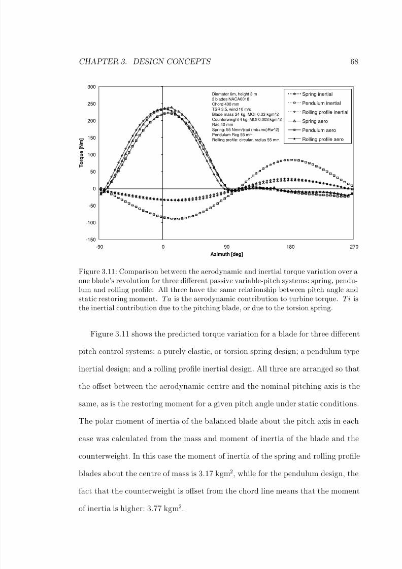
8/13/2019 Wholewhole
http://slidepdf.com/reader/full/wholewhole 93/396
CHAPTER 3. DESIGN CONCEPTS 68
-150
-100
-50
0
50
100
150
200
250
300
-90 0 90 180 270
Azimuth [deg]
T o r q u e [ N m ]
Spring inertial
Pendulum inertial
Rolling profile inertial
Spring aero
Pendulum aero
Rolling profile aero
Diamater 6m, height 3 m
3 blades NACA0018Chord 400 mm
TSR 3.5, wind 10 m/s
Blade mass 24 kg, MOI 0.33 kgm^2
Counterweight 4 kg, MOI 0.003 kgm^2
Rac 40 mm
Spring: 55 Nmm/(rad (mb+mc)Rw^2)
Pendulum Rcg 55 mm
Rolling profile: circular, radius 55 mm
Figure 3.11: Comparison between the aerodynamic and inertial torque variation over aone blade’s revolution for three different passive variable-pitch systems: spring, pendu-lum and rolling profile. All three have the same relationship between pitch angle and
static restoring moment. Ta is the aerodynamic contribution to turbine torque. T i isthe inertial contribution due to the pitching blade, or due to the torsion spring.
Figure 3.11 shows the predicted torque variation for a blade for three different
pitch control systems: a purely elastic, or torsion spring design; a pendulum type
inertial design; and a rolling profile inertial design. All three are arranged so that
the offset between the aerodynamic centre and the nominal pitching axis is the
same, as is the restoring moment for a given pitch angle under static conditions.
The polar moment of inertia of the balanced blade about the pitch axis in each
case was calculated from the mass and moment of inertia of the blade and the
counterweight. In this case the moment of inertia of the spring and rolling profile
blades about the centre of mass is 3.17 kgm2, while for the pendulum design, the
fact that the counterweight is offset from the chord line means that the moment
of inertia is higher: 3.77 kgm2.

8/13/2019 Wholewhole
http://slidepdf.com/reader/full/wholewhole 94/396
CHAPTER 3. DESIGN CONCEPTS 69
The predicted pitch responses at this tip speed ratio are almost identical for
the spring and rolling profile turbines. The response is slightly different for the
pendulum design due to its higher moment of inertia. The aerodynamic contribu-
tions to the torque are therefore similar. For a turbine of this solidity at this tip
speed ratio, virtually all of the torque is generated between azimuth angles of -90
and 90, in the upwind pass of the blade.
The sinusoidal variation in the non-aerodynamic torque component reflectsthe sinusoidal pitch response. The amplitude of this torque component is largest
for the pendulum design. In the case of the elastic system, the torsion spring
that provides the restoring moment exerts a reaction torque on the rotor that is
proportional to the pitch angle. The amplitude of this reaction is smaller than the
inertial reaction of the pendulum blade because the mass centre is not offset from
the pivot axis.
The predicted inertial reaction for the rolling profile system is lower than for
the pendulum design in this case. Its amplitude is slightly higher than is predicted
for the spring case. Here the offset y0 has been set to zero so that the centre of
mass lies on the circular rolling profile. Because the point of rolling contact rather
than the centre of mass does most of the movement, the reaction forces are much
lower. If some positive y0 value were used, the inertial reaction amplitude would
increase. The kinematics of the rolling profile concept are described in more detail
in Appendix A.
Customisation of profile
The application of the rolling profile concept to the wind turbine also allows the
response of the blades at different wind and rotational speeds to be tailored by the
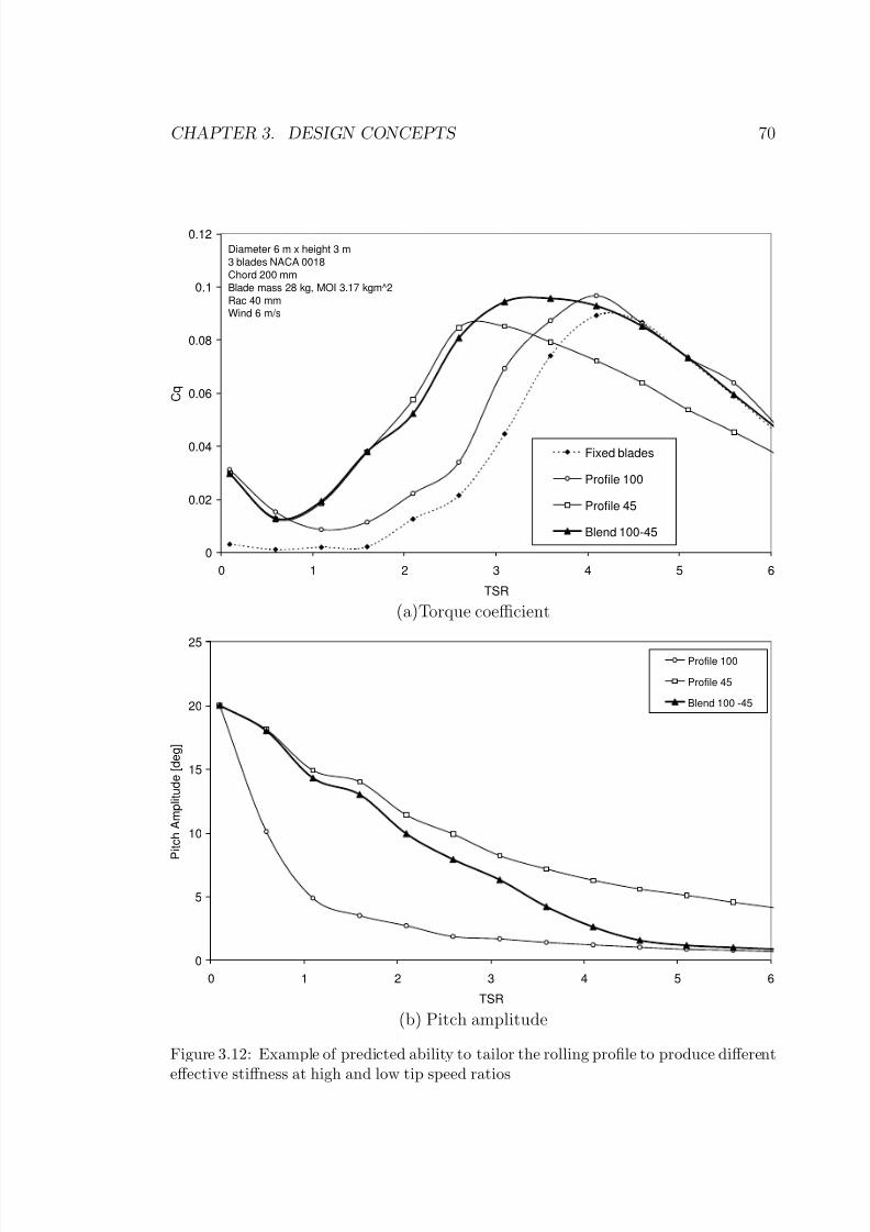
8/13/2019 Wholewhole
http://slidepdf.com/reader/full/wholewhole 95/396
CHAPTER 3. DESIGN CONCEPTS 70
0
0.02
0.04
0.06
0.08
0.1
0.12
0 1 2 3 4 5 6
TSR
C q
Fixed blades
Profile 100
Profile 45
Blend 100-45
Diameter 6 m x height 3 m
3 blades NACA 0018
Chord 200 mm
Blade mass 28 kg, MOI 3.17 kgm^2
Rac 40 mmWind 6 m/s
(a)Torque coefficient
0
5
10
15
20
25
0 1 2 3 4 5 6
TSR
P i t c h A m p l i t u d e [ d e g ]
Profile 100
Profile 45
Blend 100 -45
(b) Pitch amplitude
Figure 3.12: Example of predicted ability to tailor the rolling profile to produce different
effective stiffness at high and low tip speed ratios

8/13/2019 Wholewhole
http://slidepdf.com/reader/full/wholewhole 96/396
CHAPTER 3. DESIGN CONCEPTS 71
design of the profile. The stiffness may be made asymmetrical about the neutral
position as it may be in Kirke’s stabiliser mass design.
In addition there is the possibility of designing the profile to alter the response
at different tip speed ratios. For example, if the region surrounding the ‘nose’ of the
profile is flattened slightly, then the effective stiffness is increased over the range
of a few degrees either side of the neutral position. This change can significantly
affect the response of the blade at high tip speed ratios where the blade pitchamplitude is small, but has much less effect on the motion of the blade at slow
speeds where the amplitude is large.
The performance predicted by the momentum theory mathematical model de-
scribed in Chapter 5 for such a profile is shown in Figure 3.12(a). The predicted
performance is shown for two rolling profiles which produce under static conditions
a linear relationship between restoring moment and pitch angle. The ‘stiffest’ of
these, labelled “Profile 100”, produces a offset of d = 100 mm x θ. This profile is
predicted to achieve the best peak efficiency at high tip speed ratios. This profile
produces a pitch response whose amplitude diminishes rapidly with tip speed ratio,
shown in Figure 3.12(b). The ‘softest’ profile, Profile 45, gives a greater amplitude
at all tip speed ratios, resulting in improved intermediate speed performance, but
significantly diminished peak performance.
The predicted performance for a profile that does not produce a simple linear
relationship between restoring moment and pitch angle, but instead is ‘stiffer’ over
the range of a few degrees either side of zero, is shown as “Blend 100-45”. The
blend profile is predicted to produce the best of the stiffest and softest linear
profiles, combining the good intermediate TSR performance of Profile 45 with the
good high TSR peak performance of Profile 100. The predicted pitch amplitude

8/13/2019 Wholewhole
http://slidepdf.com/reader/full/wholewhole 97/396

8/13/2019 Wholewhole
http://slidepdf.com/reader/full/wholewhole 98/396
CHAPTER 3. DESIGN CONCEPTS 73
0
1
2
3
4
5
6
7
8
9
10
0 1 2 3 4 5 6 7 8 9 10
Pitch angle [deg]
d [ m m ]
Profile 45
Profile 100
Blend 100-45
(a) d− θ relationships
-1
0
1
2
3
4
-10 -9 -8 -7 -6 -5 -4 -3 -2 -1 0 1 2 3 4 5 6 7 8 9 10
mm
m m
Profile 100
Profile 45
Blend
(b) The corresponding rolling profiles
Figure 3.13: Comparison of the d − θ relationships for the two ‘linear spring’ profiles,labelled Profile 100 and Profile 45 and the ‘blend’ profile with d = (100−45) θ
(40 θ)2+1 + 45θ mm

8/13/2019 Wholewhole
http://slidepdf.com/reader/full/wholewhole 99/396
CHAPTER 3. DESIGN CONCEPTS 74
3.4 Experimental Work
Three new geometries were designed on the basis of the initial experimental re-
sults, the recommendations of Azim (2001) and the rolling profile design concept
described above. They are shown in Figure 3.14.
The first was designed along the same lines as the initial geometry and manu-
factured in the same grade of 60 durometer polyurethane, but modified to rectify
some of the shortcomings observed.
• The blade design was modified so that equal-sized spars that were sym-
metrical about the centre of mass were used. This allowed the elastomeric
mounting part to be made symmetrical about its centreline, eliminating the
problems of asymmetry noted earlier. This required significant modification
to blade design. An endplate was added that allowed the forward spar to be
placed outside the blade section profile.
• The two curved arms of the original design were replaced with a single stem
at the centreline. This produced a lower sectional moment of inertia and so
lower bending stiffness for the same cross sectional area. This was an attempt
to minimise the torsional stiffness while maximising the tensile stiffness.
• The end of the part was made curved instead of flat. This was designed to
produce a more gradual stiffening once end contact did occur, by providing
a contact patch that grew as the compressive load increased.
This geometry is hereafter referred to as ‘Type A’. It is shown in place on the
turbine in Figure 3.15 and in the test rig in Figure 3.16.
The other two geometries were based on a combination of the elastomeric and
rolling profile concepts described above in Sections 3.2 and 3.3. They were made
from a harder grade of polyurethane, of 90 durometer hardness, than the Type A

8/13/2019 Wholewhole
http://slidepdf.com/reader/full/wholewhole 100/396
CHAPTER 3. DESIGN CONCEPTS 75
TYPE A
TYPE B
TYPE C
Figure 3.14: The three second-generation blade mounting part geometries.

8/13/2019 Wholewhole
http://slidepdf.com/reader/full/wholewhole 101/396

8/13/2019 Wholewhole
http://slidepdf.com/reader/full/wholewhole 102/396
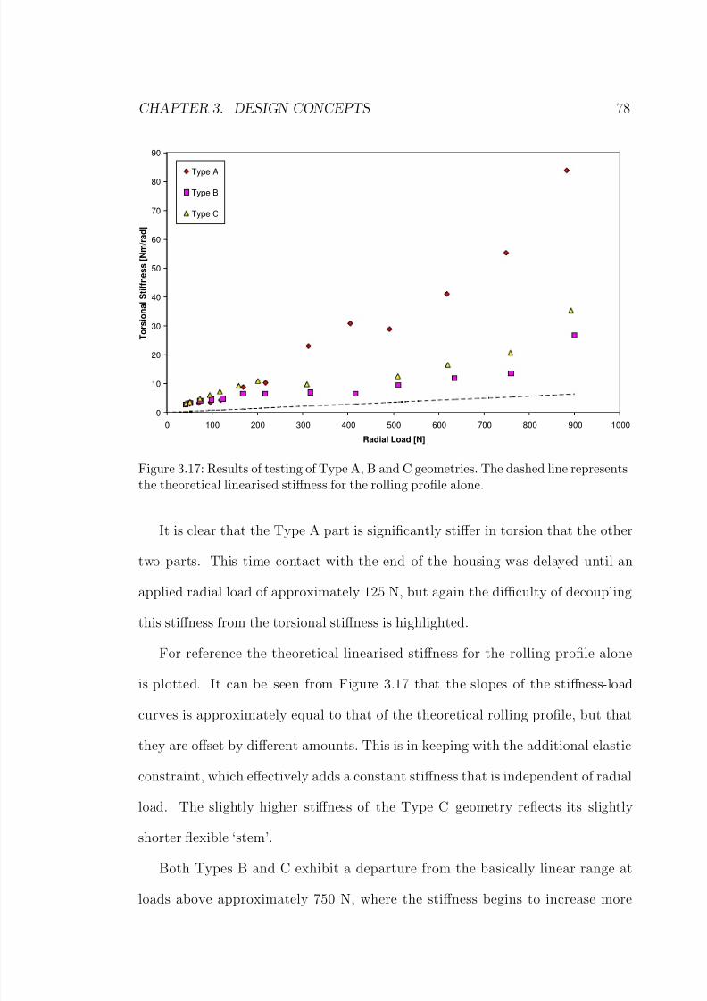
8/13/2019 Wholewhole
http://slidepdf.com/reader/full/wholewhole 103/396
CHAPTER 3. DESIGN CONCEPTS 78
0
10
20
30
40
50
60
70
80
90
0 100 200 300 400 500 600 700 800 900 1000
Radial Load [N]
T o r s i o n a l S t i f f n e s s [ N m / r a d ]
Type A
Type B
Type C
Figure 3.17: Results of testing of Type A, B and C geometries. The dashed line representsthe theoretical linearised stiffness for the rolling profile alone.
It is clear that the Type A part is significantly stiffer in torsion that the other
two parts. This time contact with the end of the housing was delayed until an
applied radial load of approximately 125 N, but again the difficulty of decoupling
this stiffness from the torsional stiffness is highlighted.
For reference the theoretical linearised stiffness for the rolling profile alone
is plotted. It can be seen from Figure 3.17 that the slopes of the stiffness-load
curves is approximately equal to that of the theoretical rolling profile, but that
they are offset by different amounts. This is in keeping with the additional elastic
constraint, which effectively adds a constant stiffness that is independent of radial
load. The slightly higher stiffness of the Type C geometry reflects its slightly
shorter flexible ‘stem’.
Both Types B and C exhibit a departure from the basically linear range at
loads above approximately 750 N, where the stiffness begins to increase more

8/13/2019 Wholewhole
http://slidepdf.com/reader/full/wholewhole 104/396
CHAPTER 3. DESIGN CONCEPTS 79
rapidly. The reason for this additional stiffening is not known, but it may be due
to compression of both parts at the rolling contact. This will be discussed further
in Section 10.4.4.
3.5 Conclusion
Two distinct design concepts were conceived to allow the blade pitch response to
be tailored on the basis of theoretical results. Each of these concepts differs from
existing designs in the degree of control they offer over the relationship between
blade restoring moment and centrifugal load.

8/13/2019 Wholewhole
http://slidepdf.com/reader/full/wholewhole 105/396
Chapter 4
Development of a Pro/MECHANICA model of a passive
variable-pitch turbine
4.1 Introduction
Preliminary investigation of passive variable-pitch turbine performance and dy-
namics was conducted using the commercial motion simulation software package
Pro/MECHANICA, produced by Parametric Technology Corporation - website
http://www.ptc.com. The package is used within the School of Mechanical and
Manufacturing Engineering at UNSW in the Pro/ENGINEER integrated mode.
Pro/MECHANICA is able to simulate the motion of the turbine rotor and
blades over time as a multi-degree-of-freedom mechanism under the influence of
prescribed loads. It was used to investigate the general performance of the pen-
dulum type inertial design and to gain insight into the dynamics of this type of
turbine.
4.2 Pro/MECHANICA Model
Parts are created and assembled in Pro/ENGINEER, then converted to a mecha-
nism with the desired degrees of freedom within Pro/MECHANICA.
The model created in Pro/ENGINEER and used in Pro/MECHANICA is
shown in Figure 4.1. It was designed to represent the essential features of the
turbine and the manner in which they are connected.
80

8/13/2019 Wholewhole
http://slidepdf.com/reader/full/wholewhole 106/396
CHAPTER 4. DEVELOPMENT OF A PRO/MECHANICA MODEL 81
Figure 4.1: Pro/MECHANICA model of the pendulum type inertial turbine

8/13/2019 Wholewhole
http://slidepdf.com/reader/full/wholewhole 107/396
CHAPTER 4. DEVELOPMENT OF A PRO/MECHANICA MODEL 82
In the initial version of the model, the rotor body was connected to the base
via a “pin joint”, giving it one rotational degree of freedom. The base is fixed
as “ground”. Each of the three blades is connected to the rotor by a pin joint,
making the mechanism planar.
Each blade consists of two discs whose diameter and thickness can be adjusted
to achieve any combination of mass and polar moment of inertia. The aerofoil-
shaped features are massless surfaces and are purely cosmetic. One disc representsthe mass of an unbalanced blade, centred at the aerodynamic centre of the aerofoil
profile. As before, the distance between the aerodynamic centre and the pin joint
axis is termed Rac. The position of the other disc is adjusted so that the combined
centre of mass lies on a line perpendicular to the blade chord line passing through
the pivot axis. The offset of the centre of mass from the pivot axis is labelled Rcg.
This arrangement causes the blade to seek a zero pitch angle under the action of
centrifugal force.
This double disc model was designed to reflect the fact that blade mass and
polar moment of inertia are constrained by structural design considerations, and
so the parameters Rac and Rcg cannot be adjusted independently.
Later the model was given two additional degrees of freedom of horizontal
translation of the rotor hub. This freedom was designed to represent the flexibility
of the turbine tower, so that the potential significance of this motion on the blade
pitch response may be investigated.
4.2.1 Aerodynamic load simulation
While Pro/MECHANICA is well suited to investigation of the dynamics of the
turbine mechanism, it is not designed to simulate aerodynamic loads. The aero-
dynamic forces experienced by each of the blades were approximated using a

8/13/2019 Wholewhole
http://slidepdf.com/reader/full/wholewhole 108/396
CHAPTER 4. DEVELOPMENT OF A PRO/MECHANICA MODEL 83
combination of the standard loads available in Pro/MECHANICA based on two-
dimensional blade element theory.
Pro/MECHANICA allows the user to create a set of “measures”, which are
either kinematic variables such as joint axis positions or velocities, or are values
calculated from these via user-entered expressions. The values of measures are
computed at each time step and can be used to control the magnitudes of loads
applied to the mechanism.For this analysis, measures were created to compute the magnitude and direc-
tion of the apparent wind on each blade at each time step, based on the blade’s
own velocity and the free wind velocity. The angle of attack, which takes into
account the blade’s instantaneous pitch angle, is then used to find the value of
measures for lift, drag and pitching moment coefficients from a lookup table of
values published for the NACA 0018 profile (Lazauskas, 2002).
Further measures are computed for the magnitude of lift and drag forces on
each blade, based on the relative wind speed. It is not possible to adjust the
direction of a force in Pro/MECHANICA during a run. Therefore the variable
direction of the lift and drag forces on each blade was simulated using a set of
four fixed force components. These forces are fixed in direction relative to the
World Coordinate System (ground) and together can simulate any direction and
magnitude of resultant force. They are applied to the aerodynamic centre of each
blade, assumed to be fixed at the quarter chord. The key measures defined for
each blade are shown in Table 4.1.
In this simplified analysis no account is taken of any reduction in wind ve-
locity due to the force transmitted to the flow by the blades (so no energy is
extracted from the air), nor for the effects of dynamic stall, flow curvature, finite

8/13/2019 Wholewhole
http://slidepdf.com/reader/full/wholewhole 109/396
CHAPTER 4. DEVELOPMENT OF A PRO/MECHANICA MODEL 84
Measure Definition
U Free wind velocitySet manually prior to run
theta Rotor azimuth angle.= Joint Axis Measure
azimuth Theta normalised to 0 to 2π.= mod(theta + blade.theta0, 2π)
pivot Blade pitch angle.= Joint Axis Measure
blade.theta0 Azimuth angle offset fromthe reference blade for this blade.
Set manuallyV Speed of the blade.
= if(omega<1e-5, 0, omega x radius)Wx X component of the relative wind at the blade.
= -V cos(azimuth)Wy Y component of the relative wind at the blade.
= V sin(azimuth) - UW Magnitude of relative wind.
= sqrt(Wx2 + Wy2)zp.alpha Angle of attack on zero pitch blade.
= if(W <1e-5, 0,if(V <1e-5, -π/2− azimuth,if(mod(azimuth, π) == π/2,if(V < U && mod(azimuth, 2π) == π/2, -π, 0),if(cos(azimuth)< 0, acos((W 2 + V 2 − U 2)/(2W V )),-acos((W 2 + V 2 − U 2)/(2W V )))))
alpha Actual angle of attack.= zp.alpha - pivot
AoA alpha normalised to 0 to 360.= (alpha - 2π floor(alpha/(2π)) x 180/π
Cl Lift coefficient.= Look-up table, input AoACd Drag coefficient.
= Look-up table, input AoADx Drag force due to Wx
= 0.5 rho chord span Wx W CdLx Lift force due to Wx
= 0.5 rho chord span Wx W ClDy Drag force due to Wy
= 0.5 rho chord span Wy W CdLy Lift force due to Wy
= 0.5 rho chord span Wy W Cl
Table 4.1: Key Pro/MECHANICA measures. Relevant measures are duplicated for eachblade.

8/13/2019 Wholewhole
http://slidepdf.com/reader/full/wholewhole 110/396
CHAPTER 4. DEVELOPMENT OF A PRO/MECHANICA MODEL 85
aspect ratio, wind shear or parasitic drag. These simplifications were considered
justifiable because the aim of the exercise was to investigate the dynamics of the
turbine rather than assess its efficiency. The assumption of constant wind veloc-
ity is significant not so much because of the consequent overestimation of average
output torque (this could be corrected), but because of the variation in wind ve-
locity both across the width of the turbine and between upwind and downwind
passes that is neglected. This variation significantly effects the pitch cycle whenthe turbine is heavily loaded and the wind is greatly decelerated. Therefore the
Pro/MECHANICA simulations were confined to low tip speed ratios and corre-
spondingly small loads, where deceleration of the flow is minimal.
The turbine speed was chosen to give a relatively low tip speed ratio of 1.3 at
a wind speed of 6 m/s. This speed is also in the operating region of interest for a
study of self-starting ability.
4.3 Summary
A simplified model of a pendulum type inertial passive variable-pitch turbine was
created in Pro/MECHANICA. The model may be used to study the dynamics of
this type of turbine under the influence of simplified aerodynamic loads. As no
account of flow deceleration is made, the model is not useful for predicting the
operating output of the turbine, except at very low speeds. This model was used
to conduct initial investigations of the relationships between key design parameters
and blade pitch response. Results of its use are presented in Chapter 7.

8/13/2019 Wholewhole
http://slidepdf.com/reader/full/wholewhole 111/396
Chapter 5
Development of a Momentum Theory Mathematical Model
for Passive Variable-Pitch Darrieus Turbines
5.0.1 Background of momentum models
The development of momentum theory models for VAWTs has been discussed
in Section 2.2.1. The model produced here was based on the Double Multiple
Streamtube method set out by Sharpe (1990).
Momentum theory (or more specifically Blade Element/Momentum (BEM)
theory) is based on obtaining two expressions for the streamwise force on the
rotor. The force is given by the rate of change of momentum of the flow, which is
equal to the overall change in velocity times the mass flow rate. The force is also
equal to the average pressure difference across the rotor. Bernoulli’s equation is
applied separately to the flow upstream and downstream of the rotor, assuming
energy is lost from the flow only at the rotor. These two equations produce the
well-known result that the overall flow velocity change is twice the velocity change
that has occurred by the time the flow passes the rotor.
Expressed in terms of the widely used ‘flow induction factor’ a, if the flow
velocity at the rotor U is defined as
U = U ∞(1 − a) (5.1)
86
8/13/2019 Wholewhole
http://slidepdf.com/reader/full/wholewhole 112/396
CHAPTER 5. MOMENTUM THEORY MODEL 87
where U ∞ is the free stream velocity, then the final flow velocity in the far wake
U w is:
U w = U ∞(1 − 2a) (5.2)
This result relates the streamwise force on the rotor to the flow velocity at the
rotor.
A second expression relating these quantities is obtained using blade-element
theory. The flow velocity at the blade is used to calculate the angle of attack and
the known aerodynamic properties of the blade section are used to calculate the
resulting streamwise force. Simultaneous solution of these two equations allows
the calculation of the blade loads and the flow velocity given the blade speed and
orientation. This is done using an iterative procedure.
In order to accommodate the variation in velocity across the rotor, the width
is divided into a number of independent streamtubes, for each of which the mo-
mentum balance is carried out separately.
The Double Multiple Streamtube version developed by Paraschivoiu (1981)
models the turbine’s interaction with the wind in the upwind and downwind passes
of the blades separately. The assumption is made that the wake from the upwind
pass is fully expanded and the ultimate wake velocity has been reached before the
interaction with the blades in the downwind pass. The downwind blades therefore
see a reduced ‘free-stream’ velocity. This approach more accurately represents the
variation in flow through the turbine.
5.0.2 Present extension
In the present work, the two-dimensional Double Multiple Streamtube model for
Darrieus turbines has been extended to incorporate the prediction of blade pitch

8/13/2019 Wholewhole
http://slidepdf.com/reader/full/wholewhole 113/396
CHAPTER 5. MOMENTUM THEORY MODEL 88
response for a passive variable-pitch turbine. While similar work has been con-
ducted by Bayly and Kentfield (1981) and Kirke and Lazauskas (1993), their work
was limited in application to the specific design conceived by the respective au-
thors. In order to evaluate particular designs and also to examine passive pitch
systems more generally (so that different and new designs may be compared), a
model that allowed for different methods of pitch control was required.
Accordingly the present model is able to deal with 5 different types of pitchcontrol:
• General elastic pitch control, in which the blade is free to pivot about a
specified point on the chord line, is balanced so that the centre of mass lies
on the pivot axis and pitch is controlled by a torsion spring whose stiffness
is a function of the turbine speed.
• ‘Pendulum’ type inertial pitch control, as designed by Sicard (1977), Kent-
field (1978) and Brenneman (1983).
• ‘Stabiliser mass’ type inertial pitch control, based on the principle of the
designs of Liljegren (1984) and Kirke and Lazauskas (1987).
• ‘Rolling profile’ type inertial pitch control, as described in Section 3.3
• ‘Cycloturbine’ type cam-driven preset pitch schedule, for comparison pur-
poses. This includes fixed-pitch standard Darrieus turbines.
Any combination of the above passive pitch control types can be handled, for
example a pendulum type inertial system can be supplemented with some elastic
pitch control. The kinematics of these designs is discussed in Appendix A.
5.0.3 Basis of the mathematical model
In the Double Multiple Streamtube model for the Darrieus turbine, the flow
through the rotor is divided into a number of independent streamtubes. In this
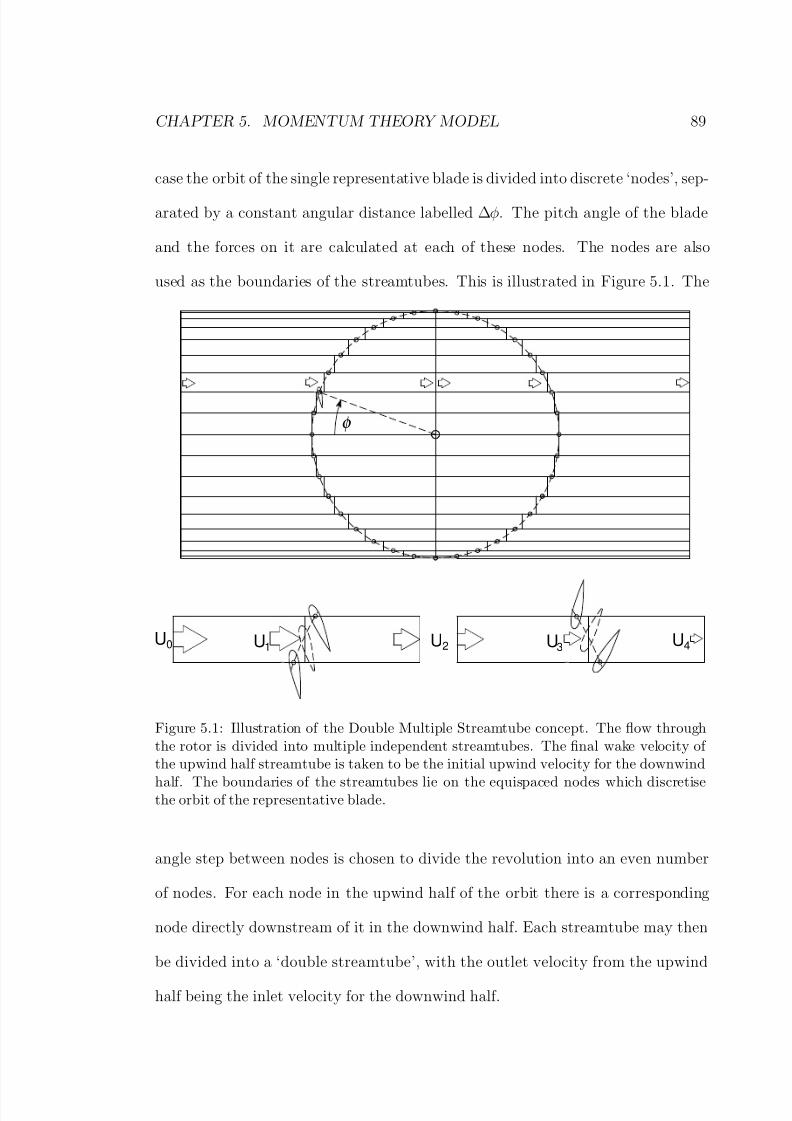
8/13/2019 Wholewhole
http://slidepdf.com/reader/full/wholewhole 114/396
CHAPTER 5. MOMENTUM THEORY MODEL 89
case the orbit of the single representative blade is divided into discrete ‘nodes’, sep-
arated by a constant angular distance labelled ∆φ. The pitch angle of the blade
and the forces on it are calculated at each of these nodes. The nodes are also
used as the boundaries of the streamtubes. This is illustrated in Figure 5.1. The
φ
U0 U U2 U U41 3
Figure 5.1: Illustration of the Double Multiple Streamtube concept. The flow throughthe rotor is divided into multiple independent streamtubes. The final wake velocity of the upwind half streamtube is taken to be the initial upwind velocity for the downwind
half. The boundaries of the streamtubes lie on the equispaced nodes which discretisethe orbit of the representative blade.
angle step between nodes is chosen to divide the revolution into an even number
of nodes. For each node in the upwind half of the orbit there is a corresponding
node directly downstream of it in the downwind half. Each streamtube may then
be divided into a ‘double streamtube’, with the outlet velocity from the upwind
half being the inlet velocity for the downwind half.

8/13/2019 Wholewhole
http://slidepdf.com/reader/full/wholewhole 115/396
CHAPTER 5. MOMENTUM THEORY MODEL 90
For a standard Darrieus turbine, the blade orientation within each streamtube
is a function only of the azimuth angle. For a variable-pitch Darrieus turbine
however, the additional degree of freedom means that the angle of attack for the
segment cannot immediately be calculated and used for the iteration procedure
described above. Instead, the blade pitch is affected by the aerodynamic forces
on the blade, and the calculation of its position must be incorporated into the
iteration. The process used is shown in Figure 5.2.The motion of the blade and the forces on it are tracked around the orbit
starting from the point at which the blade is advancing directly into the wind, at
azimuth φ = −90. Each node is then handled in sequence, so that the upwind
half of the orbit is completed and the outlet velocities are calculated and available
to be used as the inlet velocities for the downwind half.
At each node, the velocity experienced by the blade there is taken to be that
for the streamtube it is about to cross. An initial flow induction factor is assumed
for the streamtube, usually zero, and the resulting forces on the blade calculated
based on its current orientation.
Blade force is calculated using blade-element theory. The blade is treated as
a two dimensional aerofoil profile and published lift, drag and pitching moment
coefficients for the section are used to calculate aerodynamic forces and moments
based on the angle of attack, relative flow velocity and blade Reynolds number.
The coefficients for the NACA 0018 section used here are the data of Sheldahl and
Klimas (1981), corrected by Lazauskas (2002). They provide data for the full 360
range of angle of attack at Reynolds numbers from 40,000 to 500,000.
Unsteady aerodynamics, including dynamic stall, greatly affect the perfor-
mance of Darrieus turbines, especially at the low tip speed ratios that are the

8/13/2019 Wholewhole
http://slidepdf.com/reader/full/wholewhole 116/396
CHAPTER 5. MOMENTUM THEORY MODEL 91
Calculate the pitching moment on the blade for the induced wind
Assume a value of the flow induction factor,
speed found from a
a
Calculate instantaneous aerodynamic loads and the resulting changein pitch and pitch velocity over time interval t∆
Use the average pitch angle for the streamtube to calculate the
streamwise force from blade element theory, Fbe
Compare Fbe with the force Fm calculated by momentum theory using
the current value of the flow induction factor
Calculate an updated value of the flow induction factor,
Is the change in less
an+1from the
difference between Fm and Fbe , to use for next iteration
a
a
than ?acritical
Accept current value of as correct for the streamtube
NO
YES
Figure 5.2: Iterative procedure used to calculate the flow velocity and blade motionwithin a streamtube
8/13/2019 Wholewhole
http://slidepdf.com/reader/full/wholewhole 117/396
CHAPTER 5. MOMENTUM THEORY MODEL 92
focus of the present work. Detailed discussion of the treatment of unsteady aero-
dynamics, for both the momentum and vortex models, is given in Section 5.1.
Once the aerodynamic loads have been calculated, the instantaneous pitching
acceleration resulting from aerodynamic forces, any elastic forces and inertial forces
is then calculated. The pitching acceleration depends on the kinematics of the
particular variable-pitch design. Kinematics are treated in detail in Appendix A.
For example, the instantaneous pitching acceleration for a blade of the ‘pen-dulum’ inertial type of Sicard (1977) and Kentfield (1978) is given by:
θ =
M − Rcg sin θmR φ2 − (I cg + mR 2
cg) + mRcgR cos θ φ
I cg + mR 2cg
(5.3)
where
M is the total aerodynamic and elastic moment acting on the blade;
Rcg is the offset of the centre of gravity from the pivot axis; R is the turbine
radius; θ is the current pitch angle and φ is the turbine speed. I is the polar
mass moment of inertia of the blade assembly about the centre of gravity and m is
the blade assembly mass. Note that for the assumption of constant turbine speed
made for the momentum model, the term in the numerator proportional to turbine
acceleration φ vanishes.
A fourth-order Runge-Kutta numerical integration scheme (de Vahl Davis,
1991) is used to predict the pitch and pitching velocity for the blade at the next
node, on the other side of the streamtube. The blade orientation at the midpoint
of the streamtube is then estimated using the mean of the initial and final pitch
angles (i.e. constant pitching velocity across the streamtube is assumed). The
angle of attack based on this pitch angle at the midpoint is then used to calculate
the blade element aerodynamic force for the streamtube. The difference between

8/13/2019 Wholewhole
http://slidepdf.com/reader/full/wholewhole 118/396
CHAPTER 5. MOMENTUM THEORY MODEL 93
blade element force and the momentum derived force for the assumed flow in-
duction factor is then calculated and used to generate a new estimate of the flow
induction factor. Here Newton’s method (de Vahl Davis, 1991) is used to find the
zero crossing of the function that is the difference between momentum and blade
element estimates of streamwise force. The independent variable is the flow in-
duction factor a. The process is repeated until the change in flow induction factor
between iterations is acceptably small.Once the flow induction factor iterations have converged and the blade pitch
and velocity at the next node have been predicted, the forces on the blade at the
current node are finalised and stored.
This process is repeated for each node until the entire revolution has been
completed. Since the whole procedure began with an arbitrarily assumed pitch
and pitching velocity (usually both zero), calculation must continue for several
revolutions until a steady-state pitching pattern has been established. Equilibrium
is checked by comparing the initial and final pitch angles and velocities, as well as
the integrated torque for the revolution.
5.1 Unsteady Aerodynamics including Dynamic Stall
5.1.1 Introduction
Unlike the blades of a horizontal axis turbine, VAWT blades experience a con-
stantly changing angle of attack and flow velocity even under steady operating
conditions. While the static aerodynamic properties of the aerofoil sections typ-
ically employed for the blades are well documented, prediction of loads under
dynamic conditions remains difficult.

8/13/2019 Wholewhole
http://slidepdf.com/reader/full/wholewhole 119/396
CHAPTER 5. MOMENTUM THEORY MODEL 94
The difference between static and dynamic loads is dependent on the rate of
change of the angle of attack and is significant for Darrieus turbine operation. Noll
and Ham (1982) state that maximum aerodynamic loads may be as much as three
times greater under dynamic conditions than under static conditions, while the
peak pitching moment may be up to five times greater.
Many authors (Klimas, 1982; Noll and Ham, 1982; Paraschivoiu and Allet,
1988; Jiang et al., 1991) emphasise the importance of accounting for unsteadyaerodynamic loads from the perspective of structural design, fatigue life and drive-
chain and generator sizing. The effect on overall turbine performance may also
be significant. In general, the increased peak loads and delayed stall that are
associated with dynamic conditions lead to an improvement in performance over
that predicted using only static characteristics. Paraschivoiu and Allet state that:
“[The effects of dynamic stall] can be seen in particular on the
power performance curves, which exceed the steady-flow prediction for
tip speed ratios of less than four. The ability to predict dynamic stall
is therefore of crucial importance for optimising the Darrieus wind
turbine.”
Thus unsteady aerodynamics and specifically dynamic stall are important to
the study of the low tip speed ratio performance of Darrieus turbines. While a
passive variable-pitch turbine is designed to reduce the incidence of stalling at
intermediate tip speed ratios, stall is inevitable at start-up and the timing and
magnitude of the associated aerodynamic loads and moments can have a significant
impact on the blade pitch history for the entire revolution. The average torque
and not just the peak load is therefore sensitive to stall behaviour. Consequently

8/13/2019 Wholewhole
http://slidepdf.com/reader/full/wholewhole 120/396
CHAPTER 5. MOMENTUM THEORY MODEL 95
it is vital that unsteady aerodynamics be incorporated in any mathematical model
of a passive variable-pitch turbine.
The following section covers the basic features of unsteady turbine blade aero-
dynamics and the available methods of quantifying their effect on turbine perfor-
mance.
5.1.2 Attached flow unsteady aerodynamics
Unsteady aerodynamic forces may be divided into circulatory and non-circulatory
components.
Circulatory unsteady effects
Unsteady circulatory effects for attached flow are:
• the change in circulation about the aerofoil due to the influence of vorticity
in the wake;
• the change in circulation about the aerofoil due to the motion of the foil.
The latter effect is commonly included by calculating the circulation based on
the angle of incidence at the 3/4 chord location, rather than the quarter chord lo-
cation. Since the blade is rotating about the turbine axis and possibly also about
its own pivot axis, the angle of incidence varies along the chord line. Fung (1955)
presents a quasi-steady analysis of lift and drag for use in aeroelastic analysis,
using classical thin aerofoil theory, where the influence of unsteady wake vorticity
is neglected. He shows that for an aerofoil that is both pitching and plunging, the
lift is proportional to the angle of attack at the 3/4-chord position. He presents
a further analysis for an oscillating aerofoil without the quasi-steady assumption,
based on complex potential flow and conformal mapping of a circle to a flat plate.
This analysis confirms the significance of the 3/4-chord point, which Fung terms
the “rear aerodynamic centre”. Strickland et al. (1981) use a similar complex po-
tential flow analysis for a flat plat in general motion presented by Milne-Thomson

8/13/2019 Wholewhole
http://slidepdf.com/reader/full/wholewhole 121/396
8/13/2019 Wholewhole
http://slidepdf.com/reader/full/wholewhole 122/396
CHAPTER 5. MOMENTUM THEORY MODEL 97
edged vertical gust. This analysis is based on the influence of the unsteady wake of
the aerofoil, assumed to be planar (or linear, in the two-dimensional case) behind
the foil.
Unsteady wake effects on attached flow behaviour may be incorporated using
a semi-empirical unsteady aerodynamics model such as the Beddoes-Leishman
model described in Section 5.1.3. However the complexity of the wake in the
Darrieus turbine case makes the task of such methods very difficult. This topic isdiscussed further in the context of the free vortex mathematical model described
in Chapter 6.
Non-circulatory unsteady effects
Non-circulatory aerodynamic loads are generally termed “added mass” forces.
They arise from the acceleration of air due to blade motion and exist even in
the absence of a free stream.
By contrast, Leishman and Beddoes (1986) use piston theory to calculate the
non-circulatory, or impulsive, load on the blade. It is assumed to arise from a
compression wave on one side of the blade with an expansion wave on the other,
and allows the effects of compressibility to be included, which is important for
helicopter applications, but should not be significant for wind turbines.
Quantification of unsteady effects in attached flow
Strickland et al. (1981) cite an analysis by Milne-Thomson (1968) for forces on a
moving and rotating flat plate in potential flow. This analysis yields expressions
for the additional circulation around the aerofoil due to its rotation, as well as the
added mass forces that are independent of circulation. This results in expressions
for the total normal and tangential (chordwise) forces. The tangential force is
found to be proportional to the angle of attack at the mid-chord position. The

8/13/2019 Wholewhole
http://slidepdf.com/reader/full/wholewhole 123/396
CHAPTER 5. MOMENTUM THEORY MODEL 98
normal force consists of a term that is proportional to the angle of attack at the
3/4-chord position and an added mass term proportional to the normal acceleration
of the foil. Strickland et al. state that an order-of-magnitude analysis justifies the
omission of this added mass term. Likewise, the added mass pitching moment
term is judged to be small.
They conclude that unsteady pitching and added mass effects may be treated
in practice by:
• calculating the tangential force using the angle of attack at the mid-chord in
the static look-up table of aerodynamic coefficients for the section;
• calculating the normal force similarly using the 3/4 chord angle of attack;
• assuming the pitching moment about the quarter-chord is negligible for at-
tached flow.
This method has been adopted for both the momentum model and the vortex
wake model described in Chapter 6.
Unsteady wake effects have been neglected in the momentum model due to
the complexity of the wake structure and the difficulty in using a semi-empirical
model based on a linear wake to represent its influence. Wake effects are modelled
explicitly in the vortex model.
5.1.3 Dynamic stall
At zero incidence, a symmetric aerofoil generates no lift. As the angle of attack
increases, the lift increases in an approximately linear fashion, until at a critical
angle the flow begins to separate from the upper surface of the foil. Flow separation
leads to the sudden loss of lift and increase in drag that is termed stall.
The angle at which stall occurs depends on the rate of change of the angle of
attack. Traditionally, published lift and drag coefficients for an aerofoil section are

8/13/2019 Wholewhole
http://slidepdf.com/reader/full/wholewhole 124/396
CHAPTER 5. MOMENTUM THEORY MODEL 99
obtained from measurements made under quasi-static conditions. Under dynamic
conditions stall occurs at a higher angle of attack than under static conditions,
with an associated increase in the maximum lift attained. This phenomenon is
termed dynamic stall.
Stage 1: Airfoil exceeds static stall angle, thenflow reversals take place in boundary layer.
Stage 2: Flow separation at the leading−edge, followedby the formation of a ’spilled’ vortex. Moment stall.
Stage 2−3: Vortex convects over chord, it inducesextra lift and aft center of pressure movement.
Stage 3−4: Lift stall. After vortex reaches trailing−edge, theflow over upper surface becomes fully separated.
Stage 5: When angle of attack becomes low enough, the flowreattaches to the airfoil, front to back.
−0.3
−0.2
−0.1
0
0.1
0 5 10 15 20 25
UnsteadyStatic
1
2
3
4
5
0
0.5
1
1.5
2
0 5 10 15 20
25
UnsteadyStatic
1
23
4
5
0
0.1
0.2
0.3
0.4
0.5
0.6
0 5 10 15 20 25
UnsteadyStatic
Angle of attack − deg.
3
4
251
L i f t c o e f f i c i e n t , C l
M o m e n t c o e f f i c i e n t , C m
D r a g c o e f f i c i e n t , C d
Figure 5.3: Schematic showing the features of the dynamic stall process. Reproducedfrom Leishman (2002)
Dynamic stall is characterised by the formation of a distinct vortex on the
upper side of the aerofoil that detaches from the leading edge region and convects
downstream over the surface of the foil. The convection of this vortex produces
a rearward motion of the centre of pressure and a corresponding negative peak in
pitching moment about the quarter chord. Once the dynamic stall vortex travels
8/13/2019 Wholewhole
http://slidepdf.com/reader/full/wholewhole 125/396
CHAPTER 5. MOMENTUM THEORY MODEL 100
past the trailing edge, lift drops sharply and the flow is fully separated. Upon
return to lower angles of attack, reattachment of the flow may be delayed to a
significantly lower angle than that at which separation occurred. These features
are illustrated in Figure 5.3, reproduced from Leishman (2002).
Considerable experimental attention has been devoted to the topic of dynamic
stall by measuring forces and pressure distributions on pitching aerofoils in the
wind tunnel (for example Daley and Jumper, 1984; Francis and Keesee, 1985;Strickland and Graham, 1986; Lorber and Carta, 1988; Niven and Galbraith, 1997;
Gracey et al., 1996, 1997). It is clear from this work that the magnitude of the
delay of stall and the peak loads attained is a function of the pitch rate. There
is however some disagreement in the literature as to the exact nature of this re-
lationship. Lorber and Carta (1988) concluded from their experiments at low
pitch rates that the angle at which moment stall occurs is linearly dependent on
the pitch rate. However Gormont (1973) proposed a correlation that is based
on Theodorsen’s theory and is extended using experimental data from oscillating
aerofoil tests. It suggests that the stall delay angle is related to the square root
of the non-dimensionalised pitch rate. Experimental work by Daley and Jumper
(1984), Francis and Keesee (1985) and Strickland and Graham (1986) appear to
confirm this relationship. More recent work at the University of Glasgow (for
example Niven and Galbraith, 1997; Gracey et al., 1996, 1997) suggests a combi-
nation of the two. For pitch rates that are high enough for fully dynamic stall,
characterised by the formation of the stall vortex, the stall delay was found to
be linearly proportional to pitch rate. At lower pitch rates, the stall is termed
“quasi-steady”, with no discernible stall vortex. In this region, their stall delay
correlation includes a square root term.

8/13/2019 Wholewhole
http://slidepdf.com/reader/full/wholewhole 126/396
CHAPTER 5. MOMENTUM THEORY MODEL 101
Semi-empirical dynamic stall Models
Most of the work on the dynamic stall phenomenon appearing in the literature has
been conducted by researchers in helicopter aerodynamics. Empirical dynamic stall
models that have been applied to Darrieus wind turbines are the Massachusetts
Institute of Technology (MIT) method (Johnson, 1970), Gormont or Boeing-Vertol
method (Gormont, 1973), ONERA method (Petot, 1989) and Beddoes-Leishman
(Leishman and Beddoes, 1986, 1989) method.
The MIT method was modified by Noll and Ham (1982) to include the empir-
ical representation developed by Boeing-Vertol for the dynamic stall angle. They
applied the method to the performance prediction of the variable-pitch Pinson
‘cycloturbine’ VAWT.
Boeing-Vertol - The Gormont, or Boeing-Vertol model is a simple empirical re-
lation commonly used for Darrieus turbine analysis. The original Boeing-Vertol
model was modified by Strickland et al. (1979) for use with their vortex code. It
was used by Paraschivioiu et al. (1988) in their Double Multiple Streamtube code.
The model assumes that the lift-curve slope and the zero-lift angle for the
aerofoil are unchanged by dynamic effects and it is the angle at which stall occurs
and the peak lift coefficient attained that are modified. Effectively the linear region
of the lift curve slope is extended beyond the static stall angle. A modified angle
of attack is found for use in a look-up table of static lift and drag coefficients.
The degree of stall delay is assumed to be proportional to a reduced pitch rate
parameter cα
2W
where c is blade chord length, α is the rate of change of angle of attack and W is
the relative wind speed.

8/13/2019 Wholewhole
http://slidepdf.com/reader/full/wholewhole 127/396
CHAPTER 5. MOMENTUM THEORY MODEL 102
Paraschivoiu (1983) compared aerodynamic forces predicted by a Double-Multiple
Streamtube model incorporating the Boeing-Vertol dynamic stall model with ex-
perimental data from a small straight-bladed Darrieus turbine in the wind tunnel.
He reported small differences in the magnitude of the predicted steady state power
coefficient when the dynamic stall model is included, but significant differences in
instantaneous blade loads. He concluded that while the dynamic stall model pro-
vided large improvement over the static model, the results were still different fromexperimental data. The difficulty of obtaining accurate instantaneous force mea-
surements should however be remembered.
The Boeing-Vertol model was implemented in both the momentum and vortex
models presented here. The criteria for its use suggested by Strickland et al.
(1979), that it be turned on when the angle of attack is above static stall or when
the angle is decreasing below stall having been above it, were adopted.
It was found that this model caused significant reduction in the estimated
torque, compared with the use of static lift and drag, at tip speed ratios where the
maximum angle of incidence just exceeds the static stall angle. A small excursion
beyond the designated static stall angle does not allow much time for increased
peak lift before the angle of attack starts to decrease again, at which point the
modified angle switches to be greater than the geometric angle and delays the
reattachment of flow until angles much lower than the static stall angle. This phe-
nomenon of delayed reattachment has been observed in experiments (for example
Wickens, 1985).
Kirke (1998) used a momentum model for a passive-pitching VAWT that in-
corporated the Boeing-Vertol model as modified by Cardona (1984). Cardona
recommended two modifications to the model used by Strickland:
8/13/2019 Wholewhole
http://slidepdf.com/reader/full/wholewhole 128/396
CHAPTER 5. MOMENTUM THEORY MODEL 103
1. that dynamic stall not be considered when the model predicts rapidly oscil-
lating angle of attack and that the static coefficients be used instead;
2. that the average of the static and predicted dynamic values of lift and drag
coefficients be used when the angle of attack is much greater than the stall
angle.
The second modification was a response to the observed overprediction of peak
tangential force by his free vortex VAWT model compared with the experimental
results of Strickland et al. (1981).
The first modification may have been a method for dealing with the numerical
instability that the vortex model is prone to when a rapid change in angle of attack
occurs. This will be discussed in more detail in Section 6.3.
Details of the model are given in Appendix B.
MIT - Noll and Ham (1982) modified the original MIT model developed by John-
son (1970) for application to wind turbines and presented predicted results for a
small Darrieus turbine. Details of the method are given in Appendix B.
The original MIT method was developed for helicopter aerodynamics. It was
based on the delay of stall to a prescribed elevated angle of attack at which point
peak values of lift and moment were instantaneously attained and held until the
angle of attack began to decrease again. The coefficients then decayed exponen-
tially with time until the static stall angle was reached. The values of the peak
lift and moment were given as a function of the reduced pitch rate
αc
W
derived from experimental results.

8/13/2019 Wholewhole
http://slidepdf.com/reader/full/wholewhole 129/396
CHAPTER 5. MOMENTUM THEORY MODEL 104
Noll and Ham modified the method to calculate the dynamic stall angle using
the Boeing-Vertol empirical method, in which the stall delay is a function of the
square root of the reduced pitch rate.
Static sectional coefficients are used while the angle of attack is below static
stall. When it exceeds static stall but is still below dynamic stall, C L is calculated
from
C L =
as sin
α (5.4)
where as is the lift curve slope at static stall. When the dynamic stall angle is
reached the dynamic stall vortex is assumed to commence its motion from the
leading edge. In this region the lift coefficient continues to be calculated from
Equation (5.4) until either it reaches an empirically derived maximum value, or
the angle of attack starts to decrease again.
In Noll and Ham’s method the attainment of peak angle of attack marks the
commencement of the exponential decay of lift and pitching moment coefficients
from the peak value down to the static stall values.
A number of modifications to this method to make it suitable for application
to the starting performance of Darrieus turbines are suggested. These are detailed
in Appendix B.
Beddoes-Leishman - The Beddoes-Leishman method is based on an indicial aero-
dynamic response function, which is defined as the response to a step change
between two steady-state conditions. The theory is that if the indicial response
is known, the total response to an arbitrary time history of input (i.e. angle of
attack) can be obtained using superposition.
The model is composed of three distinct sections:

8/13/2019 Wholewhole
http://slidepdf.com/reader/full/wholewhole 130/396
CHAPTER 5. MOMENTUM THEORY MODEL 105
• an attached flow region;
• a separated flow region where the effect of trailing edge separation is mod-
elled;
• a dynamic stall region, where the effect on lift and moment of the formation,
convection and detachment of the dynamic stall vortex are modelled.
Beddoes and Leishman used an indicial response function for the normal force in
attached flow on an aerofoil composed of two parts: a non-circulatory component
that acts instantaneously and then decays exponentially towards zero; and a circu-
latory component builds up from zero to asymptotically approach the steady state
value. Time constants for these processes are obtained empirically for a specific
aerofoil shape and a range of Mach numbers.
5.1.4 Comparisons
Paraschivoiu and Allet (1988) compared predictions from the Boeing-Vertol dy-
namic stall model and those from the MIT model as modified by Noll and Ham
(1982) with experimental data from the Sandia 17m turbine for the normal force
and average torque. Both models overestimated the maximum normal force on the
upwind side of the rotor, but the MIT model successfully predicted no dynamic
stall on the downwind pass, whereas the Boeing-Vertol model did. Paraschivoiuand Allet point out that Noll and Ham assume that the coefficients return to the
linear (unstalled) domain when the angle of attack returns to below the static stall
angle, however the experimental data indicates that flow remains separated until
well below static stall.
The experimental data was from free wind operation and the tip speed ratio was
not stated. The Boeing-Vertol method’s use in the Double Multiple Streamtube

8/13/2019 Wholewhole
http://slidepdf.com/reader/full/wholewhole 131/396
CHAPTER 5. MOMENTUM THEORY MODEL 106
model was limited to those zones determined to have low turbulence from water-
tunnel observations. Turbulence is stated to delay the dynamic stall phenomenon
and the static aerofoil characteristics are used where turbulence is high.
Major and Paraschivoiu (1992) preformed a comparison between the Gormont,
MIT and an indicial method based on the Beddoes-Leishman model and exper-
imental data from the Sandia 17m turbine. They found that for some cases the
indicial and Gormont methods predicted the occurrence of dynamic stall when theMIT model agreed with experiment in predicting a static stall case. Nevertheless
they concluded that the indicial method offers a better representation of dynamic
stall than the other two, thus allowing more accurate local blade load prediction.
5.1.5 Summary
Three dynamic stall models were implemented in the code for the momentum
theory model and the vortex theory model to be described in Chapter 6. These
were:
• The Boeing-Vertol method;
• The Boeing-Vertol model with modifications suggested by Cardona;
• The MIT model modified by Noll and Ham.
Details of these methods are given in Appendix B. The three models were im-
plemented for comparison and are selectable via the GUI in the program. The
Beddoes-Leishman model has not been implemented because it was not clear that
its much greater complexity would result in greater stability and accuracy. How-
ever this model, or any improved model that is developed in the future, could be
implemented as an additional module.
8/13/2019 Wholewhole
http://slidepdf.com/reader/full/wholewhole 132/396
CHAPTER 5. MOMENTUM THEORY MODEL 107
5.2 Sample Results
The momentum theory model was used to generate predictions of power coefficient
for a passive variable-pitch turbine. The results from three dynamic stall models
are shown in Figure 5.4.
The significant difference between the three dynamic stall models is clearly
visible at tip speed ratios less than 5.5 for the case of fixed blades and 4.5 for the
variable-pitch turbine. All three models produce significant increase in predicted
power coefficient for the TSR range 1 to 3 compared with the static case where
dynamic stall is ignored. At higher speeds the MIT model tends to converge with
the static prediction, while the Boeing-Vertol model predicts first a lower C p before
converging at a higher TSR.
At intermediate tip speed ratios the dynamic stall models all produce an in-
crease in the predicted integrated torque for the revolution by delaying stall and
increasing the proportion of time for which flow remains attached. At higher tip
speed ratios, the Boeing-Vertol model predicts a reduced output. At these speeds
the angle of attack is, at its extremes, just exceeding the static stall angle each
revolution. The dynamic stall model is activated whenever the static stall angle
is exceeded and when the angle of attack is decreasing below stall having been
above static stall. In this operating region, this results in only a small extension
of the attached flow time when angle of attack is increasing, while dynamic stall
hysteresis, resulting in delayed reattachment of flow as the angle decreases again,
produces a net increase in the amount of time that the blades are stalled. The
integrated torque for the revolution suffers accordingly.
This phenomenon is not observed in the MIT model because it effectively
switches off when the angle of attack drops below the static stall angle. While

8/13/2019 Wholewhole
http://slidepdf.com/reader/full/wholewhole 133/396
CHAPTER 5. MOMENTUM THEORY MODEL 108
-0.05
0
0.05
0.1
0.15
0.2
0.25
0.3
0.35
0.4
0.45
0.5
0 1 2 3 4 5 6
TSR
C p
No dynamic stall model
Boeing-Vertol
Boeing-Vertol (Cardona)
MIT (mod)
Wind speed 6 m/s
Diameter 6 m
Height 3 m
3 blades NACA 0018
Chord 250 mm
Mass 28 kg
I 2.76 kgm2
Fixed blades
(a) Fixed blades
-0.05
0
0.05
0.1
0.15
0.2
0.25
0.3
0.35
0.4
0.45
0.5
0 1 2 3 4 5 6
TSR
C p
No dynamic stall model
Boeing-Vertol
Boeing-Vertol (Cardona)
MIT (mod)
Wind speed 6 m/s
Diameter 6 m
Height 3 m
3 blades NACA 0018
Chord 250 mm
Mass 28 kg
I 2.76 kgm2
Pendulum type
Rac 40 mm
Rcg 45 mm
(b) Pendulum type passive variable-pitch
Figure 5.4: Predicted power coefficient against tip speed ratio showing significant vari-
ation between dynamic stall models.

8/13/2019 Wholewhole
http://slidepdf.com/reader/full/wholewhole 134/396
CHAPTER 5. MOMENTUM THEORY MODEL 109
hysteresis is a known feature of the dynamic stall process, from these results it ap-
pears to be overestimated by the Boeing-Vertol model in this form. The Cardona
modified version mitigates this effect by simply using the mean of the modified
and static coefficients. This produces results that are more like those of the MIT
model at all speeds.
The effect of all of the dynamic stall models disappears when the tip speed
ratio is sufficiently high to keep the angle of attack below the static stall angle atall times.
The effect of the passive variable-pitch system is also clearly seen from these
results. The starting and intermediate tip speed ratio performance is significantly
improved. For this choice of parameters, the peak power coefficient is reduced
because some pitching is still occurring at the tip speed ratio at which this occurs
(approximately 4). This reduces the amplitude of the periodic variation in angle
of attack well below stall, reducing the lift produced. A trade-off between starting
and high-speed performance is necessary and may be controlled by the choice of
the blade mass centre offset parameter Rcg, which determines the strength of the
restoring moment.
5.2.1 Summary
The treatment of unsteady aerodynamic effects is the greatest difficulty facing
mathematical models of vertical-axis wind turbines. The approach of starting
with static empirical lift and drag data and modifying it according to the rate of
change of angle of attack cannot hope to accurately capture the full complexity
of the unsteady aerodynamics. However a more fundamental computational fluid
dynamics (CFD) approach remains excessively expensive and impractical in such

8/13/2019 Wholewhole
http://slidepdf.com/reader/full/wholewhole 135/396
CHAPTER 5. MOMENTUM THEORY MODEL 110
models. Accordingly the shortcomings of more economical treatments must be
tolerated.
The MIT model was favourably compared with the Boeing-Vertol model by
Paraschivoiu and Allet (1988). Comparisons with published experimental data
presented in Section 6.4 indicate the modified MIT model is the most suitable of
those tested. The Boeing-Vertol method predicts significant reduction in turbine
power when the angle of attack just exceeds the static stall angle.
5.3 Limitations of Momentum Theory
Equation 5.2 implies that if the flow is decelerated to less than half its initial
magnitude by the time it reaches the rotor, then in order to satisfy the momentum
balance, the flow velocity in the far wake must be negative and there must be a
point somewhere upstream of that at which velocity is zero. Clearly this result
is not physically realistic. Wilson and Lissaman (1974) state that the momentum
analysis should not be considered valid for a > 0.5.
In reality, the assumption of lossless expansion of the flow on the downstream
side of the rotor needed to apply Bernoulli’s equation is not justified when the rotor
is heavily loaded. When the deceleration is large, the flow through and around
the rotor becomes turbulent, resulting in significant loss of energy. This operating
state is termed the ‘Turbulent Wake State’ by Stoddard (1976). Momentum theory
predicts that as the flow induction factor increases above a = 0.5 towards a = 1 the
streamwise thrust (proportional to the pressure drop across the rotor) will decrease
towards zero. Experimental work by Glauert (1926) on free-running windmills
indicates that in fact the thrust increases in this region, until at a = 1 the thrust
is akin to that on a solid disc that allows no flow to pass through and about which
there is large scale turbulence and recirculation.

8/13/2019 Wholewhole
http://slidepdf.com/reader/full/wholewhole 136/396
CHAPTER 5. MOMENTUM THEORY MODEL 111
In order to accommodate the breakdown of momentum theory in this region the
modification suggested by Sharpe (1990) is used. A straight line is fitted through
experimental data to produce an empirical expression for the streamwise thrust
coefficient C T in terms of the flow induction factor a (see Figure 5.5).
Figure 5.5: The empirical modification to momentum theory used by Sharpe (1990) todeal with heavily loaded rotor operation
Instead of the standard expression for C T :
C T = 4a(1 − a) (5.5)
in the region aT < a < 1, C T is given by:
C T = C T 1 − 4(C 0.5T 1 − 1)(1 − a) (5.6)

8/13/2019 Wholewhole
http://slidepdf.com/reader/full/wholewhole 137/396
CHAPTER 5. MOMENTUM THEORY MODEL 112
where
aT = 1 − 0.5C 0.5T 1
and C T 1 is 1.816. This value approaches the drag coefficient for a solid disc per-
pendicular to the flow.
While this modification avoids the obvious impossibility of wake reversal and
allows the model to be used for a > 0.5, the predicted power may still not be
accurate. Stoddard (1976) states that:
“Entrance into Turbulent Wake by a wind generator brings with it
reversals in induced velocity (bound circulation along the blade), high
turbulence, vibration, and a precipitous decrease in shaft torque.”
In addition, the relationship between the pressure on the downstream side of the
rotor and the far wake final velocity is now lost, as Bernoulli’s equation cannot be
used. While for a horizontal axis rotor, this does not matter as the wake velocity
is of little concern, for the double multiple streamtube approach used here, the
wake velocity calculated from the upwind pass of the blades is used as the input
velocity for the downwind pass.
The modification allows the blade-element force iteration process to converge
to flow induction factors greater than 0.5, whereas without it no convergence can
be reached in this region due to the negative slope of the C T curve. However the
wake velocity will still be predicted as negative for a > 0.5. In reality the wake
velocity will approach zero as a approaches 1, but turbulence and recirculation
will dominate.
So while the modified momentum theory predicts smooth deceleration of the
flow right up to complete blockage, the real situation is very much more compli-
cated, and the turbine output in this operating region is likely to be significantly

8/13/2019 Wholewhole
http://slidepdf.com/reader/full/wholewhole 138/396
CHAPTER 5. MOMENTUM THEORY MODEL 113
overestimated. This fact provided further motivation for the development of a free
vortex model for turbine performance.
5.4 Summary
An extended Double Multiple Streamtube type mathematical model has been pro-
duced as part of this thesis to predict the steady-state performance of passive
variable-pitch Darrieus turbines. The model is able to handle the specific kine-
matics of five different passive designs. The inertial reactions on the rotor produced
by the pitching blades are accounted for in the model. A modified version of the
MIT model is used to treat dynamic stall.
The speed of the model enables it to be used to investigate the effects of
variation of design parameters. Use of the model to develop a parameter selection
strategy for passive variable-pitch turbines is described in Chapter 7.

8/13/2019 Wholewhole
http://slidepdf.com/reader/full/wholewhole 139/396
Chapter 6
Development of a Free Vortex Mathematical Model for
Passive Variable-Pitch Darrieus Turbines
6.1 Background to Vortex Methods
Vortex methods are a more complex and computationally expensive alternative to
blade-element/momentum methods. The benefit is that they are able to handle
more general scenarios than can momentum methods, with fewer limitations. They
have been widely applied to helicopter, HAWT and Darrieus VAWT rotor analysis.
A review of vortex methods applied to wind turbines is given by Leishman (2002).
Vortex methods assume incompressible, potential flow in the wake. A La-
grangian approach is used, tracking discrete vortex sheet segments in the wake of
the rotor. Rather than referring to momentum, the velocity at any point in the
flow field can be calculated by applying the Biot-Savart law.
6.1.1 Reasons for using a free vortex method
The free vortex wake model used here and extended for passive variable-pitch
turbines is based on the 2 dimensional method for the Darrieus turbine developed
by Strickland et al. (1979, 1980, 1981). They list the deficiencies of momentum
models as:
• The breakdown of momentum theory at large tip speed ratios;
114

8/13/2019 Wholewhole
http://slidepdf.com/reader/full/wholewhole 140/396

8/13/2019 Wholewhole
http://slidepdf.com/reader/full/wholewhole 141/396
CHAPTER 6. VORTEX THEORY MODEL 116
smooth wind conditions”, while a “nominal” C p of 0.3 is maintained in gusty condi-
tions. The time-marching free vortex method, which tracks the motion of discrete
vorticies in the wake, is naturally able to deal with transient behaviour.
A two-dimensional free vortex mathematical model for passive variable-pitch
turbines was accordingly developed. While three-dimensional vortex models have
been produced for Darrieus turbines (see Strickland et al., 1980), the added com-
puting cost and coding complexity were not considered justified in this case. The
model has been used to investigate the significance of rotor speed variation in the
prediction of starting performance and to examine the turbulent wind performance
of a turbine connected to a load. The circumstances under which the order of mag-
nitude greater computational expense justify its use over a momentum model are
also examined.
6.2 Free Vortex Aerodynamic Model
The turbine blades are represented by bound or lifting-line vortices whose strengths
are determined using aerofoil coefficient data and the calculated relative flow ve-
locity and angle of attack. The bound vortex strength ΓB is related to the flow at
the blade via the section lift coefficient:
ΓB = 12
C LcW (6.1)
where C L is the lift coefficient, c is the blade chord and W is the local relative flow
velocity. Blade stall is accommodated through the use of empirical lift, drag and
pitching moment coefficients.
In the wake, potential flow is assumed. Discrete vortices are shed into the
wake at regular intervals, whose strength is equal to the incremental change in
the bound vorticity at the blade in order to satisfy Kelvin’s theorem, namely the

8/13/2019 Wholewhole
http://slidepdf.com/reader/full/wholewhole 142/396
CHAPTER 6. VORTEX THEORY MODEL 117
DISCRETE VORTEX
WAKE
FREE
STREAM
BOUND VORTEX
Γ N
B
Γ N
B Γ N-1
B−
Γ N-1
B Γ
N-2B−
Γ N-1
B
Γ N-3
BΓ N-2
B −
−Γ N-3B Γ
N-4B
Figure 6.1: Discrete vortex representation of the unsteady blade wake
conservation of total system circulation (see Figure 6.1).
ΓW N = ΓBN
− ΓBN −1 (6.2)
The velocity induced by the shed vortices is calculated at the turbine blades
as well as at the locations of all of the wake vortices using the Biot-Savart law.
Expressed in the z = x + iy plane, the complex velocity induced by a point vortex
at z v of strength ΓW is:
q (z ) = −12πi
ΓW (z − z v)|z − z v|2
(6.3)
To remove the singularity at z v, a smoothing factor δ is used to give a finite core
radius, producing vortex ‘blobs’. The simple core function is that used by Krasny
(1987).
q (z ) = −1
2πi ΓW (z − z v)
|z − z v|2 + δ 2 (6.4)

8/13/2019 Wholewhole
http://slidepdf.com/reader/full/wholewhole 143/396

8/13/2019 Wholewhole
http://slidepdf.com/reader/full/wholewhole 144/396
CHAPTER 6. VORTEX THEORY MODEL 119
6.2.1 Treatment of unsteady aerodynamics
The same treatment methods used for the momentum model described in Sec-
tion 5.1 were used for the vortex model. There are however different factors to
be considered in the implementation of some of the semi-empirical dynamic stall
models in a free vortex scheme. Semi-empirical models such as the Boeing-Vertol
model incorporate the effect of the unsteady wake implicitly as they were developed
on the basis of tests on oscillating foils in the wind tunnel, on which the measured
forces were affected by the unsteady wake. Semi-empirical methods such as the
Beddoes-Leishman model, which were developed from a theoretical basis that at-
tempted to reflect the relevant physical processes, incorporate Duhamel summation
of Kussner function indicial responses to a discretised history of changing angle of
attack (refer to Leishman and Beddoes, 1989). As such it explicitly incorporates
the effect of the unsteady wake.
Strickland et al. (1980) stated that the treatment of unsteady circulatory lift
is handled automatically in an approximate fashion in a free vortex scheme by
the downwash induced at the blade by the discrete vortex points tracked in the
wake. The wake vorticity that is shed in response to step change in angle of attack
mitigates the magnitude of that change. As the discrete vortex convects away from
the blade, this ‘downwash’ reduces towards zero and the angle of attack approaches
a steady state value. Thus the time-dependent nature of the response is inherently
handled in an approximate way by the discrete vortex wake model, rather than by
an empirically derived analytic method.
If a semi-empirical unsteady aerodynamic model is applied where the wake vor-
ticity is modelled explicitly, the unsteady wake effects may in fact be treated twice.
Jiang et al. (1991) recognised this in the application of the Beddoes-Leishman

8/13/2019 Wholewhole
http://slidepdf.com/reader/full/wholewhole 145/396
CHAPTER 6. VORTEX THEORY MODEL 120
model to their fixed-wake vortex model for VAWTs. However they reconciled this
duplication by pointing out that the discrete vortex modelling of each blade’s wake
included the effect of wake influence on the other blades and on the same blade
at subsequent crossings, while the semi-empirical unsteady aerodynamics model of
course did not. They stated,
“the degree of overlap [between the two methods] is considered small
enough to be insignificant in the present analysis”.
The geometry of the wake of a wing oscillating in a wind tunnel is very different
from that in the case of the Darrieus turbine, even for similar histories of angle
of attack experienced at the blade. For the former, the wake may have sinusoidal
oscillations but is still basically linear in structure and is carried directly away
from the aerofoil. For a Darrieus turbine, especially at high tip speed ratios, the
wake is coiled into a much smaller space in the immediate vicinity of the blades
and is repeatedly crossed. Thus its influence may be expected to be significantly
different from that in the wind tunnel. If the only input to the semi-empirical
unsteady aerodynamics model is the angle of attack history, then no account can
be taken of the actual wake geometry.
For dynamic stall experiments in the wind tunnel the specified angle of attack
is the geometric angle of the chord line with the free stream velocity, accounting
for the aerofoil’s own plunging and/or pitching velocity. No account is taken of
the induced velocity or downwash at the foil due to the unsteady wake, as this
cannot be measured directly and is indeed the very factor whose influence is being
predicted.
In a discrete vortex wake model of a Darrieus turbine the influence of the
unsteady wake on the angle of attack at the blade is already calculated. If a
8/13/2019 Wholewhole
http://slidepdf.com/reader/full/wholewhole 146/396
CHAPTER 6. VORTEX THEORY MODEL 121
semi-empirical model that is validated using wind tunnel data is to be applied to
the calculation of unsteady lift on a Darrieus turbine blade then the influence of
the wake should not be included in the calculation of angle of attack, so long as
the semi-empirical model can accurately reproduce the effect of the omitted wake.
However because such models assume an essentially linear wake shape, then it is
unlikely that this will be done accurately.
Alternatively the effects of the unsteady wake could be omitted from the semi-empirical unsteady aerodynamics model and this aspect left to the influence of
the discrete vortex wake. Leishman and Beddoes (1989) model the effect of the
wake as the induction of a change in the effective angle of attack experienced at
the blade. This change affects the unsteady lift under attached flow conditions,
as well as delaying the onset of stall. This change in angle of attack is handled
automatically by the discrete vortex wake. In addition to this however, they
account for a time lag in the leading edge pressure response used to detect the
onset of leading edge stall. They state that:
“this mechanism significantly contributes to the overall delay in the
onset of dynamic stall”
Further, there is a lag in the unsteady boundary layer response that further delays
trailing edge separation. Both of these effects are separate from the wake effect
and so are not modelled by the discrete vortex wake.
Modification of the angle of attack alone also cannot produce the increased
maximum lift coefficients observed under dynamic conditions. In the Beddoes-
Leishman model, this increased lift is provided to some extent by the extension of
the linear lift slope region through the delay of trailing edge separation, but also
through the addition of lift generated by the:

8/13/2019 Wholewhole
http://slidepdf.com/reader/full/wholewhole 147/396
CHAPTER 6. VORTEX THEORY MODEL 122
“excess accumulation of circulation lift that is retained in the vicin-
ity of the airfoil. . . ”
This circulation is transferred to the dynamic stall vortex that detaches from the
leading edge and convects downstream over the upper (low pressure) surface of
the blade before being shed into the wake. This aspect of dynamic behaviour is
also not accounted for purely by modification of angle of attack. Hence ideally the
non-wake dynamic effects should still be modelled separately and the wake effects
left to the discrete vortex modelling of the wake.
The preceding discussion only applies to the circulatory lift component of the
unsteady blade loading. The non-circulatory components, such as added mass
effects, are not handled by the discrete vortex wake. Accordingly, in the present
analysis, the angle of attack history incorporating the influence of the discrete
vortex wake is used as input to the modified MIT dynamic stall model. Given the
approximate nature of the semi-empirical model, any duplication of treatment of
wake effects is regarded as insignificant.
6.3 Extension of the Vortex Method for Passive Variable-Pitch
VAWTs
The basic Darrieus free vortex model is modified here in a number of ways.
Strickland et al. (1981) used a look-up table for lift and drag coefficients against
angle of attack up to 180 for the NACA0012 section. No pitching moment coeffi-
cients were used. The aerodynamic coefficients were for a single Reynolds number.
For the Darrieus turbine, not only does blade Reynolds number change apprecia-
bly with varying wind speed and tip speed ratio, but it also changes within each
revolution. Accordingly tabulated coefficients spanning Reynolds numbers from

8/13/2019 Wholewhole
http://slidepdf.com/reader/full/wholewhole 148/396
CHAPTER 6. VORTEX THEORY MODEL 123
40,000 to 500,000 were used in the present model (data from Sheldahl and Klimas,
1981, presented in Lazauskas, 2002). At each timestep the Reynolds number based
on blade chord and local relative flow velocity, as well as the angle of attack, is
calculated. The appropriate lift, drag and pitching moment coefficients are then
obtained from the tabulated data using bi-linear interpolation.
In the present work, the model has been coded in Visual C++ for Windows.
The source code developed for this thesis is included on a CD inside the back coverof this thesis. A graphical user interface (GUI) has been implemented to facilitate
the adjustment of parameter values. An animated display (see Figure 6.2) of the
turbine and the vortex wake is generated so that the evolution of the wake and
the motion of the blades can be viewed.
Figure 6.2: Screen capture of the animated output of the free vortex model
Strickland et al. (1979) used a prediction-correction method to calculate the
strength of the bound vortex at each time step. The induced velocity at the
blade element is calculated using the wake vortex positions and the bound vortex
strengths at the other blade elements at the previous time step; the bound vortex

8/13/2019 Wholewhole
http://slidepdf.com/reader/full/wholewhole 149/396
CHAPTER 6. VORTEX THEORY MODEL 124
strength is calculated on the basis of this induced velocity; the induced velocities
at all blade elements is then updated for these new values and the bound vortex
strengths then recalculated.
Here a full iterative scheme is used to calculate bound vortex strength at each
step. The reason for this is that problems were encountered with oscillation in
the bound vortex strength. Any sudden change in the angle of attack, and hence
change in bound vortex strength, produces a correspondingly large change in thestrength of the wake vortex of opposite sense, following Equation (6.2). This
wake vortex, which is still close to the blade at the following time step, induces a
correction in the angle of attack at the blade, causing a change in bound vortex
strength of the opposite sign. A wake vortex corresponding to this change is then
shed, continuing the oscillation at the next time step. This process is usually
instigated by the sharp change in lift occurring at blade stall. A string of wake
vortices of alternating signs then results, along with a sharply oscillating angle of
attack and lift history.
This instability is exacerbated by the use of a semi-empirical dynamic stall
method, such as the Boeing-Vertol model, which is dependent on the instantaneous
rate of change of angle of attack. If this is estimated using a simple first order
backward difference then the oscillation in lift due to oscillation in angle of attack
is amplified. A higher order backward difference estimate reduces the sensitivity
of the value to the instantaneous angle.
In order to decouple the rate of change from the latest estimate of angle of
attack completely, an approximate closed-form expression was derived. If the
effect of changing rotor speed and non-uniformity in the wind field is neglected,
the analytic expression for the instantaneous angle of attack may be differentiated

8/13/2019 Wholewhole
http://slidepdf.com/reader/full/wholewhole 150/396
CHAPTER 6. VORTEX THEORY MODEL 125
to obtain an estimate of the rate of change. The angle of attack on a blade at zero
pitch is given by:
α0 = −(γ + φ) (6.9)
γ is the clockwise angle between the chord line and the relative wind vector and
is calculated in the code by γ = atan2(−W x, −W y). W x and W y are the x and y
components of the relative wind velocity. They are given by:
W y = U y + φR sin φ
W x = U x − φR cos φ
U x and U y are the components of the free wind velocity at the current blade
position, φ is the blade’s azimuth angle and R is the turbine radius. Differentiating
(6.9) with respect to time and subtracting the pitching velocity θ:
α0 = − φ[ φR(U x cos φ − U y sin φ − φR)/W 2 + 1] − θ (6.10)
where W =
W 2x + W 2y .
This expression ignores the effect of the movement of the blade through a
non-uniform and unsteady flow field, as well as specific local events such as wake
crossings. However as the empirical angle modifying correlation for which the
value is used as an input is itself inexact, it is felt that this error is not significant.
The MIT dynamic stall model is also inherently less sensitive to the instanta-
neous rate of change of the angle of attack and was found to be more stable.
This instability was treated by placing the next vortex to be shed at the trailing
edge and including its influence in the calculation of the flow at the lifting-line.
Since the strength of the trailing edge vortex is related to the velocity it induces
at the lifting line by Equations (6.2) and (6.1), an iterative process is used to

8/13/2019 Wholewhole
http://slidepdf.com/reader/full/wholewhole 151/396
CHAPTER 6. VORTEX THEORY MODEL 126
calculate it and the bound vortex strength at each time step. This stabilises the
calculation of bound circulation. Damped simple iteration, a technique in which
each new estimate of the convergence variable is moderated by a comparison with
the previous estimate (see de Vahl Davis, 1991), is used to treat the same insta-
bility previously exhibited over successive time steps, now shown over successive
iterations at each time step.
This process also allows wake vortices to be shed less frequently than every time
step if desired. The string of vortices shed by each blade is a discrete representation
of the continuous vortex sheet that is shed as a result of the ever-changing angle of
incidence experienced by the blade through each revolution. It is the nature of this
representation that a large number of vortices of small strength is not necessarily
preferable to a smaller number of vortices of greater strength. It has been shown by
Moore (1981) that dividing the sheet into more vortices only serves to exacerbate
the problems of instability that eventually appear in the modelling of the roll-up
of such sheets. In addition, CPU time increases with the square of the number
of vortices. Therefore it is desirable to make the time interval between shedding
of vortices larger than the time step required for accurate numerical integration
of the equations of motion of the turbine mechanism, even with a fourth-order
scheme.
It was discovered however that decoupling the vortex and turbine motion in-
tegration time steps caused problems. Because the velocity induced by a vortex
blob according to Equation (6.4) is inversely proportional to the distance from
it, its effect on the velocity at the lifting line diminishes as it is convected away
from the blade. If a vortex is shed at each time step, the closest (most recently
shed) vortex is always at approximately the same distance from the lifting line and
so the effect is relatively smooth. If a vortex is shed only every third time step,
wake vorticity for three time intervals is accumulated in a single vortex blob and

8/13/2019 Wholewhole
http://slidepdf.com/reader/full/wholewhole 152/396
CHAPTER 6. VORTEX THEORY MODEL 127
when it is shed, there is a significant and abrupt change in the flow induced at
the lifting-line. This effect decays as the vortex is convected away until another
vortex is shed and another spike in the angle of attack at the lifting-line occurs.
By maintaining a trailing edge vortex whose strength is calculated iteratively
to satisfy Equation (6.2) at each time step, the spikes in the flow produced each
time a vortex is shed are smoothed. The trailing edge vortex is shed into the wake
after a set interval, to be replaced by a new trailing edge vortex, initially of zero
strength. This method effectively represents the most recently shed portion of the
blade wake by a discrete vortex blob at the trailing edge.
The blade incidence history may be further smoothed by representing this
nearest wake region using straight vortex sheet segments, in the manner of Fink
and Soh (1978). The two most recently shed free wake vortices are replaced by
straight vortex sheet segments joining them and the trailing edge, (see Figure 6.1)
in the calculation of the velocity induced at the lifting-line. These segments are
desingularised in the same manner as the vortex blobs, as suggested by Krasny
(1987). This ensures that the sensitivity of the lifting-line circulation to the wake
strength is not exaggerated by the concentration of the most recently shed part at
the trailing edge.
6.4 Validation Using Published Results
Several researchers have compared their vortex models with the experimental re-
sults obtained by Strickland et al. (1981). A rotor with 1, 2 or 3 straight fixed-pitch
blades of NACA 0012 section was tested in a water tow tank. The turbine had
the following parameters:

8/13/2019 Wholewhole
http://slidepdf.com/reader/full/wholewhole 153/396
CHAPTER 6. VORTEX THEORY MODEL 128
Blade chord 9.14 cm
Turbine diameter 1.22 m
Blade length in water 1.1 m
Tow tank depth 1.25 m
Strain gauges were used to measure the normal and tangential forces on the blades.
Dye injection in the water was used to observe the ‘streak line’ of particles passing
over the trailing edge. Images of the streak lines were compared with predicted
wake structures from the VDART2 program. Reasonable agreement between an-
alytical and experimental results was achieved, though some areas of discrepancy
existed. The primary area of difficulty appears to lie with the dynamic stall model.
Strickland resorted to modifying the empirically derived stall delay time constants
of the Boeing-Vertol model in order to obtain better agreement with experimental
data. Even so there are major areas of discrepancy and no single set of values
could be found to best fit all tested operating points.
Cardona (1984) published results from a modified vortex model that included
the effects of flow curvature and modified the application of the Boeing-Vertol
dynamic stall model. He claimed this improved agreement, though there are still
regions of significant discrepancy.
Ponta and Jacovkis (2001) recently developed a vortex model incorporating a
finite element calculation of the blade forces and near flow field. The free vortex
model is used to compute the ‘macro’ flow field and its results are used as boundary
conditions for the ‘micro’ local blade model, which is based on a finite element
solution of the constant-curl Laplacian equation. The velocities in each region
are calculated iteratively at each time step to find the bound vorticity. Surface
pressures and shear forces calculated by a viscous boundary layer model are then

8/13/2019 Wholewhole
http://slidepdf.com/reader/full/wholewhole 154/396
CHAPTER 6. VORTEX THEORY MODEL 129
-2
-1
0
1
2
3
4
5
6
1080 1125 1170 1215 1260 1305 1350 1395 1440 1485 1530
Azimuth [deg]
F T +
Experiment (Strickland)
Static
Boeing-Vertol
Boeing-Vertol (Cardona)
MIT (mod)
MIT (Noll & Ham)
-50
-40
-30
-20
-10
0
10
20
30
1080 1125 1170 1215 1260 1305 1350 1395 1440 1485 1530
Azimuth [deg]
F N +
Experiment (Strickland)
Static
Boeing-Vertol
Boeing-Vertol (Cardona)
MIT (mod)
MIT (Noll & Ham)
Figure 6.3: Comparison of predicted non-dimensionalised tangential and normal forcesFT + and F N + for three different dynamic stall treatments with the experimental dataof Strickland et al. (1981). 1 blade, TSR = 5.

8/13/2019 Wholewhole
http://slidepdf.com/reader/full/wholewhole 155/396
CHAPTER 6. VORTEX THEORY MODEL 130
-2
-1
0
1
2
3
4
5
1080 1125 1170 1215 1260 1305 1350 1395 1440 1485 1530
Azimuth [deg]
F T +
Experiment (Strickland)
Static
Boeing-Vertol
Boeing-Vertol (Cardona)
MIT (mod)
MIT (Noll & Ham)
-20
-15
-10
-5
0
5
10
15
1080 1125 1170 1215 1260 1305 1350 1395 1440 1485 1530
Azimuth [deg]
F N +
Experiment (Strickland)
Static
Boeing-Vertol
Boeing-Vertol (Cardona)
MIT (mod)
MIT (Noll & Ham)
Figure 6.4: Comparison of predicted non-dimensionalised tangential and normal forcesFT + and F N + for three different dynamic stall treatments with the experimental dataof Strickland et al. (1981). 2 blades, TSR 2.5

8/13/2019 Wholewhole
http://slidepdf.com/reader/full/wholewhole 156/396
CHAPTER 6. VORTEX THEORY MODEL 131
used to compute blade forces. The circulatory and added mass effects are thus
accounted for naturally and there is no reliance on experimental static aerofoil
coefficients. The finite element model however is only applied prior to stall. Once
separation is detected, the method reverts to the standard vortex model using
aerofoil coefficients and so the issue of dynamic stall, which appears to be the
most problematic, is not addressed. Nevertheless the results obtained for normal
and tangential blade forces and wake structure visualisation show good agreementwith Strickland’s experimental data.
Tangential and normal force predictions for two tip speed ratios tested by
Strickland et al. are shown in Figures 6.3 and 6.4. The degree of agreement
in general is reasonable considering the simplifying assumptions made. Primary
among these is the assumption of 2 dimensionality, which is dubious as the exper-
imental rig had a blade length of 1.1 m and a gap of 15 cm to the bottom of the
tank. The effect of the trailing tip vortex is not accounted for in the model.
Results for the dynamic stall models implemented in the code are compared.
These are the Boeing-Vertol model; the Boeing-Vertol model as modified by Car-
dona; the MIT model as modified by Noll and Ham; and the MIT model with
present modifications. All of the above models were used in conjunction with
the measures to account for finite aspect ratio, flow curvature and dynamic ef-
fect. Included for reference are the predictions using the unmodified static section
coefficients.
For the TSR = 5 case shown in Figure 6.3 none of the dynamic stall models
are able to accurately predict the upwind (left hand half of the graph) pass peak.
The Boeing-Vertol model overestimates the peak and then predicts a significant
undershoot to negative values on the descending side that does not appear in

8/13/2019 Wholewhole
http://slidepdf.com/reader/full/wholewhole 157/396
CHAPTER 6. VORTEX THEORY MODEL 132
the experimental values. The Cardona modification mitigates this effect, but still
underpredicts the duration of the peak. Noll and Ham’s MIT model underpredicts
the size of the peak and then exhibits an extended period of almost zero tangential
load that does not occur in the experiment. This is the post-stall region in which
the tangential load would be exactly zero were it not for the slight angle of attack
and drag coefficient modifications for finite aspect ratio and flow curvature. The
modified MIT method designed to remedy this shows improved but still imperfectagreement with measured values. The descending portion of the tangential force
curve around azimuth = 1200 shows artifacts of the model’s representation of lift
decay and flow reattachment after stall that appears to be problematic. The MIT
models give by far the best agreement with experimental values for tangential force
in the downwind pass (azimuth 1260 - 1440).
Note that if no account is taken of dynamic effects then the upwind tangential
force peak is greatly truncated, indicating stall.
All three models give good agreement with normal force data at TSR = 5,
though the fact that these forces are an order of magnitude greater than the
tangential loads makes the agreement appear better. Again all three models have
difficulty matching the smooth decline from the negative peak at azimuth 1170
(the upwind most point of the orbit) that was measured by Strickland et al.. The
measured values seem to indicate that no blade stall occurred at this TSR, despite
the fact that if no dynamic stall model is used, the tangential and normal force peak
in the upwind half of the revolution is truncated to less than half of the measured
peak, indicating flow separation. All the literature surveyed on dynamic stall
indicated the presence of significant hysteresis in lift, drag and moment coefficients,
with reattachment delayed to lower angles of attack than under static conditions.

8/13/2019 Wholewhole
http://slidepdf.com/reader/full/wholewhole 158/396
CHAPTER 6. VORTEX THEORY MODEL 133
This separation and delayed reseparation is apparently triggered when the angle
of attack reaches a maximum and starts to decrease, even if stall would not have
occurred at this angle had pitching continued beyond it. The experimental results
seem to indicate that flow separation has not occurred at any stage, despite the
excursion to angles greater than the static stall angle. This phenomenon is not
predicted by any of the dynamic stall models examined. Nevertheless the quality
of agreement is reasonable.Agreement for the TSR = 2.5 case shown in Figure 6.4 is not as good, with all
dynamic stall models overpredicting the upwind tangential force peak at azimuth
1160. The Cardona modified Boeing-Vertol model show and the modified MIT
model show best agreement here, but the MIT model shows much better agreement
over the rest of the revolution.
The MIT models show the best level of agreement for normal force. Again the
inadequacy of ignoring dynamic effects at this TSR are highlighted.
Figures 6.5 and 6.6 show comparisons between vortex model predictions with
the various dynamic stall models and the experimental results published by Paraschivoiu
(1983). He presented normal and tangential force coefficient data for a small
straight-bladed turbine operating in air.
Blade chord 6.1 cm
Turbine diameter 0.61 m
Blade length 0.61 m
Blade section NACA 0018
In general the level of agreement with these results is not as good as with
those of Strickland et al. The modified MIT model gives a marginally better
prediction of the measured results than the other models, however there are still

8/13/2019 Wholewhole
http://slidepdf.com/reader/full/wholewhole 159/396
CHAPTER 6. VORTEX THEORY MODEL 134
-3
-2
-1
0
1
2
3
4
1350 1395 1440 1485 1530 1575 1620 1665 1710
Azimuth [deg]
F T +
Experiment
Boeing-Vertol
Boeing-Vertol (Cardona)
MIT (mod)
MIT (Noll & Ham)
-20
-15
-10
-5
0
5
10
15
1350 1395 1440 1485 1530 1575 1620 1665 1710
Azimuth [deg]
F N +
Experiment
Boeing-Vertol
Boeing-Vertol (Cardona)
MIT (mod)
MIT (Noll & Ham)
Figure 6.5: Comparison of predicted non-dimensionalised tangential and normal forcesFT + and F N + for three different dynamic stall treatments with the experimental dataof Paraschivoiu (1983). 2 blade, TSR = 3.

8/13/2019 Wholewhole
http://slidepdf.com/reader/full/wholewhole 160/396
CHAPTER 6. VORTEX THEORY MODEL 135
-3
-2
-1
0
1
2
3
4
1350 1395 1440 1485 1530 1575 1620 1665 1710
Azimuth [deg]
F T +
Experiment
Boeing-Vertol
Boeing-Vertol (Cardona)
MIT (mod)
MIT (Noll & Ham)
-14
-12
-10
-8
-6
-4
-2
0
2
4
6
8
1350 1395 1440 1485 1530 1575 1620 1665 1710
Azimuth [deg]
F N +
Experiment
Boeing-Vertol
Boeing-Vertol (Cardona)
MIT (mod)
MIT (Noll & Ham)
Figure 6.6: Comparison of predicted non-dimensionalised tangential and normal forces
FT + and FN + for different dynamic stall treatments with the experimental data of Paraschivoiu (1983). 1 blade, TSR 1.5

8/13/2019 Wholewhole
http://slidepdf.com/reader/full/wholewhole 161/396
CHAPTER 6. VORTEX THEORY MODEL 136
areas of significant discrepancy. The measured tangential force data for TSR 1.5 in
Figure 6.6 shows an oscillation that may be due to some vibration in the turbine.
The MIT model, both in its unmodified and modified forms, grossly overpredicts
the upwind (negative) peak in the normal force, while the Boeing-Vertol models
underpredict.
Overall it is concluded that the MIT method, with modifications described in
Appendix B, offers the best agreement with experimental results of the modelstested. However none of the models is able to capture all of the details of the
blade force histories measured in the experiment.
6.5 Limitations of Vortex Methods
While vortex methods incorporate a good deal more of the complexities of Dar-
rieus turbine aerodynamics than momentum models, they still rely on significant
simplification. Potential flow is assumed in the wake and the effect of viscosity
in the blade aerodynamics is included through empirical force coefficients. The
present model is two dimensional. For a turbine with straight blades of large as-
pect ratio, this simplification is acceptable. While the affect of finite aspect ratio
is accounted for in the modification of sectional lift and drag coefficients, span-
wise flow and trailing tip vortices have not been included. Turbine shaft or tower
shadow has also been neglected in the present model.
The primary area of limitation is still the handling of unsteady aerodynam-
ics, as it has been for more than twenty years. It is clear that researchers have
investigated many different approaches to the modelling of this area that is so
important for accurate prediction of Darrieus turbine performance. These range
from the entirely empirical to complete first-principles CFD approaches, with al-
most every possible blend of the two in between. Clearly a compromise must be

8/13/2019 Wholewhole
http://slidepdf.com/reader/full/wholewhole 162/396
CHAPTER 6. VORTEX THEORY MODEL 137
reached between accuracy and simplicity. Because the real flow is so complex, the
diminishing returns of accuracy gained for ever greater investment of effort in first
principles approaches make the use of semi-empirical methods attractive.
Even so, the free vortex method is still expensive in terms of computing re-
quirements. The repeated use of the Biot-Savart law is the main cause of this
expense. For example if 200 discrete vortices are maintained for each of three
blades, 600
2
= 360, 000 Biot-Savart induced velocity calculations are required ateach time step. The method is several orders of magnitude more time consum-
ing than the momentum method and it is not practical to perform comprehensive
optimisation studies using it. This task remains the domain of more economical
methods, for conditions under which their accuracy is known and acceptable.
6.6 Motion Simulation Model
Existing momentum theory methods assume constant turbine speed and steady-
state operation. These assumptions are limiting in the study of the self-starting
performance of passive variable-pitch turbines.
The steady-state pattern of pitch angle variation predicted under the assump-
tion of constant turbine speed may be slightly different from the actual pitch vari-
ation for a turbine with finite rotor and load inertia where speed ripple is likely to
exist. The angular acceleration of the turbine rotor affects, and is affected by, the
pitching motion of the blades.
In addition, for the study of starting performance, the turbine will naturally be
accelerating, rather than operating at steady-state. Further, the passive variable-
pitch mechanism is intended to be applied to small stand-alone systems, almost
certainly driving non-constant speed and maybe non-electrical loads. Therefore
in fluctuating wind, turbine speed will almost always be changing. Acceleration

8/13/2019 Wholewhole
http://slidepdf.com/reader/full/wholewhole 163/396
CHAPTER 6. VORTEX THEORY MODEL 138
will be shown to have significant effect on the predicted pitch pattern and on the
average torque over a single revolution.
In addition to transient blade motion, the unsteady wake may also affect aero-
dynamic loads. When the turbine is heavily loaded, the deceleration of the flow
is significant. It may take a finite time for the wake to fully develop and if the
turbine speed and the wind speed are varying, the instantanteous performance at
a given tip speed ratio may be different from that at steady state with a fullydeveloped wake.
In order to accommodate these factors, turbine acceleration must be included in
the mathematical model. It is then necessary to model the entire turbine as a single
mechanism with multiple degrees of freedom. This differs from the initial approach
of assuming a constant turbine speed (effectively infinite rotor or load inertia) and
tracking the motion of a single blade under the influences of aerodynamic, elastic
and inertial forces. This single degree of freedom system permitted the use of
Newton’s vector method to arrive at the differential equation of motion by use of
a free body diagram. If the turbine speed is allowed to vary however, it becomes
necessary to calculate the rotor acceleration at every time step, since this both
affects and is affected by the motions of all of the blades at that instant. It is
therefore no longer possible to model only a single blade and to take its motion as
representative of the remaining blades.
The principle of virtual work is much better suited to deal with this multi-
degree-of-freedom system than is Newton’s approach. It enables the motions of
interconnected bodies to be tracked without reference to any joint or constraint
forces. D’Alembert’s principle allows application of the virtual work principle to
dynamic systems by including inertia forces. The Lagrangian form of the virtual

8/13/2019 Wholewhole
http://slidepdf.com/reader/full/wholewhole 164/396
CHAPTER 6. VORTEX THEORY MODEL 139
work principle, which uses a set of generalised coordinates to describe the system
position, is used to produce a set of differential equations of motion, one equation
for each degree-of-freedom. The linear set of differential equations is solved to
calculate the instantaneous accelerations of all generalised coordinates.
A numerical integration scheme is then used to predict the change in positions
and velocities of all bodies in the system during a timestep. As for the momentum
model, a fourth-order Runge-Kutta scheme is used for this purpose.
y
x
0q
3q
2q
1q
33, I m
22, I m
11
, I m
0 I
FREE WIND
Figure 6.7: Schematic of turbine mechanism defining the generalised coordinates q for aturbine of the pendulum type.
For the pendulum type configuration studied by Bayly and Kentfield (1981)
the turbine may be modelled as an open-loop planar mechanism - effectively a

8/13/2019 Wholewhole
http://slidepdf.com/reader/full/wholewhole 165/396
CHAPTER 6. VORTEX THEORY MODEL 140
number of double pendula connected at the turbine shaft (see Figure 6.7). A set
of F = n+1 generalised coordinates is used for a turbine having n blades: one for
the pitch angle of each blade and one for the rotor azimuth angle. q 0 is defined as
the azimuth angle of the reference blade, being the clockwise angle specifying the
orbital position of the blade relative to the wind direction. q 1 to q n are the blade
pitch angles.
The notation used by Paul (1979) is adopted, but the equation is reformulatedhere in matrix form. The velocity coefficients for the M = n+1 members relate
the velocity of the mass centres of the members to the rate of change of each of
the F generalised coordinates. The coefficients are termed U , V and Ω for the x,
y and clockwise directions respectively, as defined in Figure 6.7. For example, the
coefficient U ij gives the influence of the rate of change of the generalised coordinate
q j on the x-direction velocity of the i-th member of the assembly. That is:
xi =n
j=0
U i,j · q i (6.11)
or in matrix form
x0
x1
...
xn
=
U 00 U 01 . . . U 0n
U 10 U 11 . . . U 1n
... ...
. . . ...
U n0 U n1 . . . U nn
·
q 0
q 1
...
q n
In matrix notation:
x = U · q (6.12)

8/13/2019 Wholewhole
http://slidepdf.com/reader/full/wholewhole 166/396
CHAPTER 6. VORTEX THEORY MODEL 141
The rotor centre of mass is assumed fixed at the origin and has zero velocity at
all times, so all coefficients relating to its translation are zero. The change in the
pitch angles of the blades has no kinematic effect on the rotor speed. Therefore
all coefficients concerning the rotor are zero, except that relating the generalised
coordinate for the azimuth to the rotor position, which is one.
U 0 j = V 0 j = 0 for j = 0, 1, 2,...n
Ω00 = 1
Ω0 j = 0 for j = 0, 1, 2, ...n
The velocity of the mass centre of the each blade is affected by both the rotor
azimuth and that blade’s pitch angle, but is independent of the pitch angles of
any other blade. For the ‘pendulum’ type inertial pitch control design shown with
three blades, the velocity coefficient matrices are:
U =
0 0 0 0
A(q 0, q 1) B(q 0, q 1) 0 0
A(q 0, q 2) 0 B(q 0, q 2) 0
A(q 0, q 3) 0 0 B(q 0, q 3)
(6.13)
V =
0 0 0 0
C (q 0, q 1) D(q 0, q 1) 0 0
C (q 0, q 2) 0 D(q 0, q 2) 0
C (q 0, q 3) 0 0 D(q 0, q 3)
(6.14)

8/13/2019 Wholewhole
http://slidepdf.com/reader/full/wholewhole 167/396
CHAPTER 6. VORTEX THEORY MODEL 142
Ω =
1 0 0 0
1 1 0 0
1 0 1 0
1 0 0 1
(6.15)
where
A(q 0, q i) = R cos(q 0 + φi) + Rcg cos(q i + q 0 + φi)
B(q 0, q i) = Rcg cos(q i + q 0 + φi)
C (q 0, q i) = −R sin(q 0 + φi) − Rcg sin(q i + q 0 + φi)
D(q 0, q i) = −Rcg sin(q i + q 0 + φi)
These kinematic relations may be replaced by those applicable to any other
design. These are given in Appendix A.
φi is the azimuth angle of blade i when q 0 is zero. For the three bladed turbine
φi = 0, 120, 240 for i = 1, 2, 3 respectively. The elements of these matrices must
be updated for the current values of the generalised coordinates at each timestep.
The accelerations of the mass centres of the members are also defined in terms
of coefficients. For example in the x-direction:
xi = U i +n
j=0
U i,j · q i (6.16)
The coefficients summed in the second term are the velocity coefficients defined
above. The first term is the acceleration coefficient for the i-th member, which is a
function of both the generalised velocities and displacements. In matrix notation,

8/13/2019 Wholewhole
http://slidepdf.com/reader/full/wholewhole 168/396
CHAPTER 6. VORTEX THEORY MODEL 143
the x-direction acceleration is given by:
x = U + U · q (6.17)
Similar equations exist for the y and clockwise directions. For the rotor, the
acceleration coefficients are all zero. The acceleration coefficient matrices are:
U =
0
E (q 0, q 0, q 1, q 1)
E (q 0, q 0, q 2, q 2)
E (q 0, q 0, q 3, q 3)
(6.18)
V
=
0
F (q 0, q 0, q 1, q 1)
F (q 0, q 0, q 2, q 2)
F (q 0, q 0, q 3, q 3)
(6.19)
where
E (q 0, q 0, q i, q i) = −Rcg( q 0 + q i)2 sin(q i + q 0 + φi) −
R q 02 sin(q 0 + φi)
F (q 0, q 0, q i, q i) = −Rcg( q 0 + q i)2 cos(q i + q 0 + φi) −
R q 02 cos(q 0 + φi)
All the angular acceleration coefficients are zero. Again, the form of these coeffi-
cients is specific to the pendulum type turbine. Expressions for the other types of
turbine discussed in this thesis are given in Appendix A.

8/13/2019 Wholewhole
http://slidepdf.com/reader/full/wholewhole 169/396

8/13/2019 Wholewhole
http://slidepdf.com/reader/full/wholewhole 170/396
CHAPTER 6. VORTEX THEORY MODEL 145
the q j is given by:
C j =n
i=0
(U imiU ij + V i miV ij + Ω
iJ iΩij) (6.22)
In matrix notation:
CT = U T ·m ·U + V T ·m ·V + Ω T · J ·Ω (6.23)
using the diagonal mass and inertia matrices defined as:
m =
mrotor 0 0 0
0 mblade 0 0
0 0 mblade 0
0 0 0 mblade
(6.24)
J =
J rotor 0 0 0
0 J blade 0 0
0 0 J blade 0
0 0 0 J blade
(6.25)
where the J terms are the polar mass moments of inertia about the respective
centres of mass.
The generalised inertia matrix is the square FxF symmetric matrix whose ele-
ments are defined as:
I rj =n
i=0(U irmiU ij + V irmiV ij + ΩirJ iΩij) (6.26)

8/13/2019 Wholewhole
http://slidepdf.com/reader/full/wholewhole 171/396
CHAPTER 6. VORTEX THEORY MODEL 146
in matrix notation:
I = UT ·m ·U + VT ·m ·V + ΩT · J ·Ω (6.27)
The above matrices are used to form the equation of motion derived from La-
grange’s form of d’Alembert’s principle:
ni=0
Qi − C i −
F j=1
I ij · q j
· q i = 0 (6.28)
The matrix form of the equation of motion is:
(Q−C− I · q) · q = 0 (6.29)
The instantaneous accelerations may be found by solving the equation for q. For
general velocities, Equation (6.29) requires:
(Q−C− I · q) = 0 (6.30)
The solution is found by performing Gaussian elimination on the augmented ma-
trix:
[ I | (Q−C) ]
with matrices updated for the instantaneous positions, velocities and external
forces. The position and speeds at time t+∆t can be found through numerical
integration. Here a fourth-order Runge-Kutta numerical integration scheme is
used.

8/13/2019 Wholewhole
http://slidepdf.com/reader/full/wholewhole 172/396
CHAPTER 6. VORTEX THEORY MODEL 147
6.7 Constrained Cases
For comparison purposes it is sometimes desirable to simulate the performance
either of a fixed bladed turbine whose speed is allowed to vary, or of a passive
variable-pitch turbine whose speed is held constant. For these constrained cases the
general procedure above is modified to remove the redundant degrees of freedom.
For the first case the system reverts to a single degree-of-freedom. The blades
may be fixed or their motion may be prescribed as a function of the azimuth, as for
a cycloturbine. The generalised force for the rotor degree of freedom is calculated
as normal, but an additional external load is added to account for the moment on
the blades that is now transmitted directly to the rotor and the moment required
to produce the prescribe blade motion.
For the second case, because the rotor speed is prescribed, the top row of the
normal augmented matrix is removed and the remaining rows (one for each of the
blades) are row-reduced to find the pitching accelerations.
6.7.1 Calculation of turbine torque
At any instant there is a certain torque applied to the turbine by aerodynamic
loads on the blades. Because the blades of a passive variable-pitch turbine are free
to move, not all of this torque is automatically available at the turbine shaft. The
shaft torque may be found by calculating the reaction forces acting on the rotor
itself at the blade connections. Since the Lagrangian analysis does not calculate
the internal reactions of the mechanism, these must be found by performing a
separate kineto-static analysis for each blade.
The joint reactions include the inertial loads due to the oscillating blades as well
as the aerodynamic forces on them. Both Bayly and Kentfield (1981) and Kirke
and Lazauskas (1992) neglected inertial effects of the swinging blades on the rotor

8/13/2019 Wholewhole
http://slidepdf.com/reader/full/wholewhole 173/396
CHAPTER 6. VORTEX THEORY MODEL 148
torque. Both considered the blade inertia in predicting the pitch response, but
assumed that only the aerodynamic forces on the blade contributed to torque, as
is true for a fixed bladed turbine. At high speeds and for heavy blades, fluctuating
tangential inertial loads may be significant. In a detailed study of turbine dynamics
including possible speed ripple, the inclusion of such loads may be important. Also,
while for a periodically oscillating blade at steady-state the fluctuating tangential
reaction at each blade pivot due to the inertia of the blade should integrate toalmost zero, it is possible for some net energy to be imparted or lost through
hysteresis in the aerodynamic loads.
Where the blade has a fixed pivot axis, the torque contributed by the blade
is equal to the product of the tangential reaction force at the connection and the
turbine radius. For the rolling profile type design, because the contact point moves
fore and aft, the torque contribution also involves the normal reaction force. The
total rotor torque at any instant is the sum of these contributions from all blades.
Whether or not the turbine accelerates under the influence of the torque de-
pends on the load connected to the shaft. Speed may be held constant either
through an actively controlled load or an effectively infinite inertia passive load.
If the load torque at that speed is less than the torque applied to the rotor by
the blades then the turbine will accelerate. In this case the power generated by
the turbine is split between the load and acceleration of the rotor. In either case
useful work is performed. The self-starting of the turbine is the focus of this work
and is a task that otherwise must be performed by an external energy source.
In order to obtain a measure of turbine performance that accounts for both of
these outputs, the total torque is taken to be the sum of the load torque at the shaft
and the torque used to accelerate the turbine. This is calculated as the turbine

8/13/2019 Wholewhole
http://slidepdf.com/reader/full/wholewhole 174/396
CHAPTER 6. VORTEX THEORY MODEL 149
acceleration multiplied by the total turbine and load inertia. For this purpose
the blades and rotor are considered as a single body. This provides an smoothed
estimate of the torque, as the instantaneous motion of the blades relative to the
rotor is neglected.
Alternatively, the total torque may be estimated by performing the kineto-
static analysis of the blades to find the joint reactions assuming the rotor accel-
eration to be zero. This method allows the fluctuating inertial reactions arisingfrom pitching acceleration to still be included. If these fluctuating loads happen to
integrate to some non-zero value over a complete revolution then this is included
in the torque.
6.8 Validation of Motion Simulation Code using
Pro/MECHANICA
In order to validate the motion simulation part of the code, results were compared
with those generated by the commercial motion simulation package Pro/MECHANICA.
A simplified scenario was modelled, consisting of three blades mounted on a rotor,
with a constant magnitude downwind force applied to each blade. Body masses
and moments of inertia were matched and the time step in each set at 0.02 s. A
damping moment of 0.05 Nm/rad/s was applied to the pitch axes. The radial loca-
tion of the mass centre of the blade with respect to its pivot axis was adjustable, as
was the location of the ‘aerodynamic centre’ or point of application of the constant
wind force.
The motion of the blades and the rotor was tracked for 315 time steps. The
predicted pitch angles for the three blades are shown in Figure 6.8. Note that for
clarity the vortex program’s results have been thinned, only every tenth time step

8/13/2019 Wholewhole
http://slidepdf.com/reader/full/wholewhole 175/396
CHAPTER 6. VORTEX THEORY MODEL 150
-50
-40
-30
-20
-10
0
10
20
30
0 50 100 150 200 250 300
Time Step
P i t c h A n g l e [ d e g ]
Mechanica 1
Mechanica 2
Mechainca 3
Vortex 1
Vortex 2
Vortex 3
Pitch damping b = 0.050 Nm/rad/s
315 time steps total.
Every 10th Vortex data point shown.
Figure 6.8: Comparison of Pro/MECHANICA and vortex code predicted pitch responsesfor constant wind force. Note that the vortex data has been thinned for clarity.
is shown. The maximum discrepancy in pitch angle at the end of 315 time steps is
0.33. This level of agreement gives confidence that the motion simulation module
of the vortex code is free from errors.
6.9 Comparison with Momentum Method
Simulations were run for a turbine of the pendulum type, shown in Figure 6.7,
with the parameters shown in Table 6.1. Rac is the distance from the pivot
axis to the aerodynamic centre, assumed to be at the quarter chord, and its value
determines the magnitude of aerodynamic pitching moment. Rcg is the distance
from the pivot axis to the centre of gravity of the blade assembly and it determines
the magnitude of the restoring moment on the blade.

8/13/2019 Wholewhole
http://slidepdf.com/reader/full/wholewhole 176/396
CHAPTER 6. VORTEX THEORY MODEL 151
Diameter: 6 m
Height: 3 mBlades: 3 NACA0018Rac: 20 mmRcg: 45 mmBlade chord: 400 mmmblade: 28 kgJ blade: 2.7 kgm2
J rotor: 500 kgm2
Table 6.1: Turbine parameters for DMS - vortex model comparison
The present vortex method and the Double Multiple Streamtube method de-
scribed in Chapter 5 were used to predict turbine performance at a wind speed of
10 m/s and two different tip speed ratios.
-40
-30
-20
-10
0
10
20
30
-90 0 90 180 270
Azimuth [deg]
P i t c h
[ d e g ]
DMS TSR 3.1
Vortex TSR 3.1
DMS TSR 0.9
Vortex TSR 0.9
Figure 6.9: Predicted pitch response for vortex method and Double Multiple Streamtube(DMS) method.
The predicted pitch responses are shown in Figure 6.9. At TSR = 3.1 the
turbine is at steady state, connected to a load whose torque is proportional to the
square of turbine speed. At TSR = 1 the turbine is accelerating when connected

8/13/2019 Wholewhole
http://slidepdf.com/reader/full/wholewhole 177/396
CHAPTER 6. VORTEX THEORY MODEL 152
to the same load. The steep positive slope of the torque-speed curve prevents the
turbine from having a stable operating point at this TSR. Instead it is accelerating
up to the stable operating point at TSR = 3.1
At TSR = 1 the difference in pitch response predicted by the DMS and vortex
methods is largely due to the acceleration of the turbine. When using the DMS
model to study the starting behaviour of this type of turbine, stable operation is
assumed at all speeds, even if this is not possible when connected to a realisticpassive load. The difference in pitch response between steady-state and transient
cases is clear at this TSR. The difference is partly due to the different velocity field
predicted for the transient case, but is largely due to the effect of acceleration of the
rotor. The TSR increased from 0.89 to 1.03 during the course of this revolution.
The average torque calculated for the revolution by the DMS model is 277 Nm,
while the average torque for the transient vortex case is 343 Nm, including torque
driving the load and accelerating the turbine. The significant difference between
the two values is due to the difference in pitch response, especially in the azimuth
range -90 to +90, which is the upwind half of the orbit. The greater pitch
amplitude in this region reduces the amount of time spent by the blade in stalled
conditions, increasing the time spent developing useful torque.
The difference in the pitch responses at TSR = 3.1 is largely due to the dif-
ference in the velocity fields predicted by the models. The difference in average
torque is much smaller at this speed: 438 Nm for the DMS model and 417 Nm for
the vortex model.
The torque variations for one of the blades is shown in Figure 6.10.
While the momentum model is much simpler than the vortex model, it achieves
good agreement in the calculation of integrated quantities such as average torque

8/13/2019 Wholewhole
http://slidepdf.com/reader/full/wholewhole 178/396
CHAPTER 6. VORTEX THEORY MODEL 153
-100
0
100
200
300
400
500
600
700
-90 0 90 180 270
Azimuth [deg]
T o r q u e [ N m ]
Vortex
DMS
TSR 3.1
(a)
-100
0
100
200
300
400
500
-90 0 90 180 270
Azimuth [deg]
T o r q u e [ N m ]
Vortex
DMS
TSR 1
(b)
Figure 6.10: Predicted torque variation for vortex method and Double Multiple Stream-tube (DMS) method. (a) TSR = 3.1; (b) TSR = 1.0
at steady-state. However the prediction of starting performance using a steady-
state analysis may lead to significant discrepancies, not only in the instantaneous

8/13/2019 Wholewhole
http://slidepdf.com/reader/full/wholewhole 179/396
CHAPTER 6. VORTEX THEORY MODEL 154
quantities, but also in averaged values. The free vortex model is better suited
to study of this aspect of turbine performance, which is critical to variable-pitch
turbines of this type.
6.10 Conclusion
A free vortex wake model has been developed for passive variable-pitch Darrieus
turbines. The model incorporates a motion simulation module that treats the en-
tire turbine as a multi-degree of freedom mechanism. The model provides the more
accurate and detailed aerodynamic load prediction commonly claimed for standard
vortex codes in comparison with momentum models. It also allows prediction of
transient turbine performance, which is important in the study of self-starting
ability as well as turbulent wind output.

8/13/2019 Wholewhole
http://slidepdf.com/reader/full/wholewhole 180/396
Chapter 7
Development of a Parameter Selection Strategy for Passive
Variable-Pitch Systems
7.1 Introduction
The passive variable-pitch systems examined in Chapter 3 each consist in essence
of a blade free to pitch under the influence of aerodynamic forces, regulated by
some restoring moment, be it elastic or inertial in origin. For each specific design,
the magnitudes of the aerodynamic and restoring moments may be adjusted by
selection of the values of a number of design parameters. The predicted perfor-
mance has proven to be very sensitive to the values of these parameters. A logical
basis for the selection of appropriate values was therefore sought.
7.2 Study of Blade Pitch Response Using Pro/MECHANICA
7.2.1 Introduction
The Pro/MECHANICA model of a three-bladed pendulum type passive variable-
pitch turbine described in Chapter 4 has been used to study the effect of variation
in key design parameters on the blade pitch response. The polar moment of in-
ertia of the blade assembly and the magnitude of the aerodynamic and inertial
moment arms were varied and the predicted pitch responses in a steady wind were
compared.
155

8/13/2019 Wholewhole
http://slidepdf.com/reader/full/wholewhole 181/396
CHAPTER 7. PARAMETER SELECTION STRATEGY 156
7.2.2 Simulation method
The Reynolds number for the simulations was assumed to be constant at 80,000,
based on a blade chord length of 150 mm and a free wind speed of 6 m/s. The lift
and drag coefficients used to calculate the aerodynamic forces on the blades were
those published by Lazauskas (2002) based on the data of Sheldahl and Klimas
(1981) for the NACA 0018 profile at this Reynolds number.
The model described in Chapter 4 allowed the variation of the blade polar
moment of inertia for a given mass. It also allowed the parameters Rac and Rcg to
be varied. These are the distance from the pivot axis to the aerodynamic centre
for the blade (assumed to be at the quarter chord) and the distance from the pivot
axis to the centre of mass respectively. These moment arms determine the relative
strengths of the restoring inertial moment and the driving aerodynamic moment
on the blade.
Eight different blade parameter sets were examined. The ratio of aerodynamic
moment to inertial moment was kept constant by fixing the ratio Rac : Rcg (see
Figure 7.1). The value of this ratio was arrived at by a process of trial and error
as one which produced favourable results over a range of tip speed ratios.
Each configuration tested is identified by the value of the normalised aero-
dynamic centre offset, Rac defined as Rac/c, where c is the blade chord. Here
c = 150 mm with turbine radius, R = 860 mm. The polar mass moment of inertia
of the blade assembly about the pivot axis varies with Rac as shown in Figure 7.1.
For each configuration the steady state blade pitch cycle was obtained with the
tower vibration degrees of freedom locked. Initially this was attempted by setting
an arbitrary load magnitude on the turbine shaft and an arbitrary initial turbine

8/13/2019 Wholewhole
http://slidepdf.com/reader/full/wholewhole 182/396
CHAPTER 7. PARAMETER SELECTION STRATEGY 157
ω
0
0.04
0.08
0.12
0.16
0.2
0 0.2 0.4 0.6 0.8 1
Rac /c
Rac /c = 0.137
Rac /c = 0.820
Rcg
Rac
Ipivot
[kgm2]
Figure 7.1: Definition of parameters Rac and Rcg.
velocity and allowing the turbine to proceed towards an equilibrium velocity and
pattern of pitch variation.
No equilibrium was reached without viscous damping in the blade pin joints.
A damping moment of 20 Nmm/(rad/s) was accordingly applied. It was discov-
ered that this approach still did not readily yield a steady-state operating point,
especially for large values of Rcg, with correspondingly large polar moments of
inertia.
In addition, for much of the speed range the turbine torque curve increases
sharply with speed, precluding the possibility of a stable operating point. Conse-
quently a “driver” was used to fix the turbine speed at a predetermined value and
the turbine was allowed to run until the blade pitch cycles reached steady state.
The simulation time required to reach steady-state increased with the value of
Rac of the blade configuration. The arrangements with the largest inertia required
an initially larger damping coefficient, which was then progressively reduced with
time until the final value of 20 Nmm/rad/s was reached.

8/13/2019 Wholewhole
http://slidepdf.com/reader/full/wholewhole 183/396
CHAPTER 7. PARAMETER SELECTION STRATEGY 158
Once steady-state had been reached, blade pitch cycles and driver shaft torque
histories were recorded for a simulation run of 5 seconds (500 timesteps at 0.01s)
for each configuration.
7.2.3 Results
Fixed speed steady-state tests
Figure 7.2 shows the average torque for each configuration. It was found that there
was a threshold value of Rac below which torque was (highly) negative. Above the
threshold, torque was positive, but decreased with increasing Rac to a minimum
before rising slightly again. The reason for this distribution is apparent from the
-35000
-30000
-25000
-20000
-15000
-10000
-5000
0
5000
0 0.1 0.2 0.3 0.4 0.5 0.6 0.7 0.8 0.9
T o r q u e
[ N m m
]
Rac / c
Figure 7.2: Pro/MECHANICA steady-state average torque results
steady state pitch cycles for the various configurations shown in Figure 7.3. For
all cases the pitch response is essentially sinusoidal. As Rac is decreased from the
maximum value the amplitude of the pitch response increases. However for those
cases where Rac is less than 0.137 the amplitude increases markedly and the phase
of the response changes. The sharp drop in torque that corresponds to this change

8/13/2019 Wholewhole
http://slidepdf.com/reader/full/wholewhole 184/396
CHAPTER 7. PARAMETER SELECTION STRATEGY 159
is due to the fact that the pitch response becomes significantly out of phase with
the variation in incident wind direction.
As was shown in Figure 1.4 (page 11), the angle of attack variation on a fixed
blade is almost sinusoidal for tip speed ratios greater than one. In order to maintain
angles of attack of the correct sign for positive thrust to be generated, the pitch
response of the blades must be similarly sinusoidal and, ideally, in phase with the
zero-pitch angle of attack. If the phase angle between zero-pitch angle of attackand pitch angle becomes too large, the blade then experiences angles of attack of
the wrong sign to produce lift with a forward component. Figure 7.4 shows the
variation in angle of attack on one of the blades for two of values of Rac tested. The
configuration with the greater pitch amplitude ( Rac = 0.103) is almost completely
out of phase with the zero-pitch angle of attack.
The amplitude and phase of the blade pitch responses varies with the polar
moment of inertia in a fashion consistent with the variation in natural frequency
of the blade assembly.
While the turbine speed is constant, each blade can be regarded as a pendulum
suspended in an inertial field, where centrifugal force takes the place of gravity.
Ignoring the small variation in this acceleration with radius (and so with pitch
angle) for small angles the damped natural frequency is
ωd =
mRcgR φ2
I + mR2cg
−
b
2(I + mR2cg)
2(7.1)
where m is the mass of the blade assembly; R is the turbine radius; φ is the turbine
speed; b is the pitch axis damping coefficient; I is the blade moment of inertia
about its centre of mass. For small damping the natural frequency is an almost

8/13/2019 Wholewhole
http://slidepdf.com/reader/full/wholewhole 185/396
CHAPTER 7. PARAMETER SELECTION STRATEGY 160
-90
-75
-60
-45
-30
-15
0
15
30
45
60
75
90
-90 0 90 180 270
Azimuth [deg]
P i t c h
[ d e g ]
Rac /c = 0.137
Rac /c = 0.068
Rac /c = 0.103
Rac /c = 0.820
Figure 7.3: Pro/MECHANICA steady-state pitch responses
-150
-100
-50
0
50
100
-90 0 90 180 270
Azimuth [deg]
P i t c h ,
A n g
l e o f A t t a c k
[ d e g ]
Angle of attack - fixed blade
Pitch - Rac/c = 0.137
Pitch - Rac/c = 0.103
Angle of attack - Rac/c = 0.137
Angle of attack - Rac/c = 0.103
Figure 7.4: Comparison of the Pro/MECHANICA steady-state pitch and angle of attackpatterns for two values of Rac.

8/13/2019 Wholewhole
http://slidepdf.com/reader/full/wholewhole 186/396
CHAPTER 7. PARAMETER SELECTION STRATEGY 161
linear function of the rotor speed, so frequency ratio ω/ωd is almost independent
of speed.
The blade pitch response is akin to that of a single degree-of-freedom system
being excited by an approximately harmonic driving force. While the natural
frequency is higher than the running speed (the frequency ratio is less than one),
the motion of the blades is close to being in phase with the driving aerodynamic
force. However once the natural frequency drops through and below the runningspeed, the response amplitude increases greatly and the phase angle passes through
90 toward 180. This is shown in Figure 7.5. According to Equation 7.1 the
frequency ratio is one when Rac is equal to approximately 0.1.
0
1
2
0 0.1 0.2 0.3 0.4 0.5 0.6 0.7 0.8 0.9
F r e q u e n c y R a t i o
0
30
60
90
120
150
180
P h a s e A n g l e [ d e g ]
Frequency Ratio
Calculated Phase Angle
Measured Phase Angle
Rac/c
Figure 7.5: Calculated mass-spring-damper system frequency ratio and phase angles.The pitch response phase angles estimated from the zero-crossings are also shown.
The greatest output torque achieved here is at Rac = 0.137, for which the
frequency ratio is 0.90. This point represents a trade-off between the large pitching

8/13/2019 Wholewhole
http://slidepdf.com/reader/full/wholewhole 187/396
CHAPTER 7. PARAMETER SELECTION STRATEGY 162
amplitude and small phase angles required to prevent stalling of the blades over a
significant portion of the revolution.
Variable speed steady-state tests
In order to investigate the significance of rotor speed fluctuations, further sim-
ulations were performed for two of the configurations with the driver removed.
Turbine average speed was held (approximately) constant over the 5 second run
by applying a shaft torque proportional to the square of the turbine speed, in the
style of a hydraulic load. The magnitude of the load was set so as to produce
an average torque equal to the average torque that the driver had applied when
holding the turbine at that constant speed.
Results for the these runs were almost identical to those with the driver in place.
This finding reflects the small magnitude of speed fluctuations. Fluctuations have a
three per period cycle for the three bladed turbine. It is apparent that interaction
between blades and rotor is minimal at steady-state because the effect of each
blade, which may be quite significant, tends to be cancelled out by those of the
other blades.
Transient response results
Further simulation runs were then conducted with the blades started from the
zero pitch position and allowed to progress towards steady state over 15 seconds.
This was done for two values of Rac (0.137 and 0.820), first with speed fixed at 9
rad/s and then with an initial velocity of 9 rad/s and the same hydraulic load as
before. The pitch angle histories (for one of the blades) are shown in Figure 7.6.
It can be seen that the interaction between blade and rotor for Rac = 0.137 is
minimal and steady state operation is already being approached after 15 seconds.

8/13/2019 Wholewhole
http://slidepdf.com/reader/full/wholewhole 188/396
CHAPTER 7. PARAMETER SELECTION STRATEGY 163
By comparison the pitch histories for the driver and free cases for Rac = 0.820
diverge markedly, indicating the effect on pitch of fluctuation in rotor speed.
The turbine accelerations for steady state and transient cases are shown in
Figure 7.7. For Rac = 0.137, (b), the magnitudes of the acceleration variations
are not greatly different. For Rac = 0.820 however the transient case exhibits
significantly larger acceleration peaks than the steady state case. It is also the
only case for which a regular three per revolution pattern (reflecting the threeblades) has not developed by the end of the 6th revolution. This reflects the
stronger coupling between blade pitch speed and turbine speed associated with
larger moments of inertia I pivot and greater mass centre offsets (Rcg).
While minimisation of I pivot and Rcg does not appear to be critical to steady
state performance, it does affect transient performance and especially the time
taken to adjust to a change in conditions, such as a change in wind velocity. The
performance of the turbine in the turbulent conditions inevitably encountered in
the field is likely to be highly dependent on these parameters.
Turbine shaft reaction forces
The shaft radial reaction forces predicted by Pro/MECHANICA for two parameter
sets ( Rac = 0.137 and 0.820) are shown in Figure 7.8. These results are for the
constant speed (driver) simulation runs at steady-state pitch patterns. It can
be seen that the maximum reactions are significantly higher for the turbine with
blades of greater mass moment of inertia. This indicates the significance of blade
inertial loads, showing that load fluctuations do not arise only from aerodynamic
forces.

8/13/2019 Wholewhole
http://slidepdf.com/reader/full/wholewhole 189/396
CHAPTER 7. PARAMETER SELECTION STRATEGY 164
-30
-20
-10
0
10
20
30
0 2 4 6 8 10 12 14 16 18 20 22
Azimuth [rev]
P i t c h
[ d e g ]
Driver
Free
Rac /c = 0.82
(a) Rac = 0.820
-30
-20
-10
0
10
20
30
0 2 4 6 8 10 12 14 16 18 20 22
Azimuth [rev]
P i t c h
[ d e g ]
Driver
Free
Rac /c = 0.137
(b) Rac = 0.137
Figure 7.6: Pro/MECHANICA transient pitch responses for two parameter sets for theconstant speed ‘Driver’ case and the variable speed ‘Free’ case.

8/13/2019 Wholewhole
http://slidepdf.com/reader/full/wholewhole 190/396
CHAPTER 7. PARAMETER SELECTION STRATEGY 165
-0.6
-0.4
-0.2
0
0.2
0.4
0.6
4 5 6
Azimuth [rev]
T u r b
i n e A c c e l e r a t i o n [ r a d / s / s ]
Steady State TransientRac /c = 0.82
(a) Rac = 0.820
-0.6
-0.4
-0.2
0
0.2
0.4
0.6
4 5 6
Azimuth [rev]
T
u r b i n e A c c e l e r a t i o n [ r a d / s / s ]
Steady State TransientRac /c = 0.137
(b) Rac = 0.137
Figure 7.7: Pro/MECHANICA turbine acceleration fluctuations over two consecutive
rotor revolutions for two parameter sets.

8/13/2019 Wholewhole
http://slidepdf.com/reader/full/wholewhole 191/396
CHAPTER 7. PARAMETER SELECTION STRATEGY 166
The influence of tower stiffness was investigated by freeing the two planar
translation degrees of freedom at the rotor main bearing and applying a“point-
to-point” spring load between the centre of the rotor and the centre of the base.
The motion of the turbine under different values of stiffness of this spring was
examined. The shaft load was removed and the turbine allowed to accelerate from
an initial speed of 9 rad/s at a free wind speed of 6 m/s. The most successful
set of blade parameters ( ¯Rac = 0.137) and the appropriate initial blade velocities
and positions found from the steady-state analysis were used. The predicted shaft
reaction force magnitude fluctuations for three values of spring stiffness are shown
in Figure 7.9.
0
5
10
15
20
25
30
-90 0 90 180 270
Azimuth [deg]
S h a f t R e a c t i o n F o r c e M a g n u t i d e [ N
]
Rac /c = 0.820 (Ipivot = 0.169)
Rac /c = 0.137 (Ipivot = 0.036)
Figure 7.8: Pro/MECHANICA turbine shaft reaction force magnitude fluctuations fora locked rotor axis with two different blade inertias.
The stiffest spring (300 N/mm) kept total rotor axis displacement to less than
0.1 mm, resulting in a reaction force of approximately 30 N. The softest spring
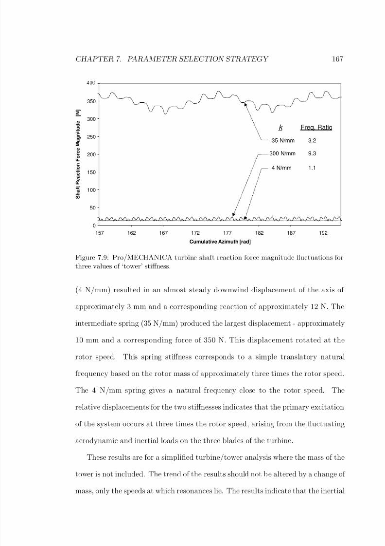
8/13/2019 Wholewhole
http://slidepdf.com/reader/full/wholewhole 192/396
CHAPTER 7. PARAMETER SELECTION STRATEGY 167
0
50
100
150
200
250
300
350
157 162 167 172 177 182 187 192
Cumulative Azimuth [rad]
S h a
f t R e a c t i o n F o r c e M a g n i t u d e
[ N ]
35 N/mm
300 N/mm
4 N/mm
k
3.2
Freq. Ratio
9.3
1.1
Figure 7.9: Pro/MECHANICA turbine shaft reaction force magnitude fluctuations forthree values of ‘tower’ stiffness.
(4 N/mm) resulted in an almost steady downwind displacement of the axis of
approximately 3 mm and a corresponding reaction of approximately 12 N. The
intermediate spring (35 N/mm) produced the largest displacement - approximately
10 mm and a corresponding force of 350 N. This displacement rotated at the
rotor speed. This spring stiffness corresponds to a simple translatory natural
frequency based on the rotor mass of approximately three times the rotor speed.
The 4 N/mm spring gives a natural frequency close to the rotor speed. The
relative displacements for the two stiffnesses indicates that the primary excitation
of the system occurs at three times the rotor speed, arising from the fluctuating
aerodynamic and inertial loads on the three blades of the turbine.
These results are for a simplified turbine/tower analysis where the mass of the
tower is not included. The trend of the results should not be altered by a change of
mass, only the speeds at which resonances lie. The results indicate that the inertial

8/13/2019 Wholewhole
http://slidepdf.com/reader/full/wholewhole 193/396
CHAPTER 7. PARAMETER SELECTION STRATEGY 168
effects of the pitching blades of this type of turbine produce fluctuating reaction
loads at the shaft, at a frequency equal to the rotor speed times the number of
blades (blade pass frequency). The magnitude of these inertial effects is dependent
on the mass moment of inertia of the blades.
7.2.4 Summary
Pro/MECHANICA was used to examine the dynamic behaviour of a pendulum
type inertial passive variable-pitch turbine. Simulations were conducted for a range
of blade parameters at a steady state operating point with a wind speed of 6 m/s
and a tip speed ratio of 1.3. It was found that best performance was obtained when
the blade parameters were set so that the natural frequency was approximately
10% higher than the rotational speed of the turbine.
Rotor speed fluctuation at steady state was found to be small and the effect on
blade pitching was negligible, due to the mutual cancellation of inertial reaction
forces at the pivots of the three blades. Under transient conditions interaction
between blades and rotor was again minimal for the best blade parameter set but
was evident for the blade with the largest moment of inertia. It is concluded that
response time to changes in wind speed will be minimised by minimisation of blade
moment of inertia (I pivot) and mass centre offset (Rcg).
Fluctuating turbine shaft reaction forces were found to be stronger for blade
arrangements with larger moments of inertia, further indicating the desirability
of minimising the blade inertia. The simulation indicates the possibility of large
displacements and reaction forces at the main bearing when the tower stiffness
places the natural frequency close to the blade pass frequency.

8/13/2019 Wholewhole
http://slidepdf.com/reader/full/wholewhole 194/396
CHAPTER 7. PARAMETER SELECTION STRATEGY 169
7.3 Parametric Study of an Elastic Passive Pitch System using the
Momentum Model
In order to undertake a more comprehensive study of parameter selection on tur-
bine performance, the momentum theory mathematical model described in Chap-
ter 5 was used. The quantities most critical to turbine performance are the strength
of the driving aerodynamic moment and the strength of the restoring moment.
These quantities are most easily examined in the context of an elastic-type passive
variable-pitch turbine, where the restoring moment is produced by a spring. In
this case adjustment of the spring stiffness does not affect the mass moment of
inertia of the blade assembly as it does in an inertial-type system.
7.3.1 Selection of restoring moment parameter
A turbine with the parameters shown in Table 7.1 was tested. These parameters
are based on those quoted by Kirke (1998) for his demonstration turbine.
Parameter ValueDiameter: 6 mHeight: 3 mBlades: 3 (NACA0018)Blade chord: 400 mmAerodynamic moment arm Rac: 25 mmInertial moment arm Rcg: 0 mm
Blade mass mblade: 28 kgBlade mass moment of inertia I : 2.55 kgm2
Damping coefficient, b: 2 Nm/(rad/s)
Table 7.1: Turbine parameters used for DMS study
The restoring moment on the blade was assumed to be provided by a torsion
spring, which applied a moment linearly proportional to the pitch angle. The
spring constant is labelled K . The steady-state performance of the turbine was

8/13/2019 Wholewhole
http://slidepdf.com/reader/full/wholewhole 195/396
CHAPTER 7. PARAMETER SELECTION STRATEGY 170
predicted at tip speed ratios (TSRs) ranging from 0.2 to 5 for different values of
K at a wind speed of 7 m/s.
0
50
100
150
200
250
300
350
400
450
500
0 1 2 3 4 5
TSR
K
[ N m / r a d ]
Cq
A
B
C
Figure 7.10: Steady-state torque coefficient C q predicted by the momentum model fora range of TSR and torsion spring constant K . Each dot represents an operating pointand C q is indicated by the colour. The three reference curves shown are:
A : K = 0.070 mbladeR φ2
B : K = 0.045 mbladeR φ2
C : K = 0.034 mbladeR φ2

8/13/2019 Wholewhole
http://slidepdf.com/reader/full/wholewhole 196/396
CHAPTER 7. PARAMETER SELECTION STRATEGY 171
Figure 7.10 shows clearly that the torsion spring stiffness K should be approxi-
mately a function of the square of the tip speed ratio. The red band of high torque
is very narrow for low speeds (TSR< 1.5), but broadens at higher speeds. At tip
speed ratios greater than approximately three, the spring stiffness may increase
toward infinity with almost no change in torque. This reflects the small pitch am-
plitude at these speeds, making the turbine behave much like a standard Darrieus
turbine (which may be regarded as having blade springs of infinite stiffness).Shown for reference are three curves representing different relationships be-
tween K and turbine speed. These are of the form K = aF R, where F R =
mbladeR φ2 is the centrifugal load on the blade and a is a constant. The significance
of the form of this relationship is that inertial pitch control systems naturally pro-
vide a restoring moment that scales with centrifugal force. If an elastic-type system
were to be used the torsional stiffness should somehow be made to increase with
centrifugal load. This is the aim underlying the elastomeric pitch control concept
explained in Section 3.2. Designs using a simple spring with a constant stiffness,
such as those of Brenneman (1983) and Leigh (1980) shown in Section 2.1.2, will
clearly not be as effective, based on these results.
An inertial system like the pendulum type of Sicard (1977) and Kentfield (1978)
has a sine relationship between pitch angle and restoring moment; however over
small angles it may be regraded as linear. An inertial system may then be regarded
as equivalent to an elastic system in which the stiffness increases with centrifugal
force. These results indicate a clear basis for implementing such a torsion spring
stiffness function.
If the spring constant can be made to vary in such a fashion with rotor speed
then significant torque can be developed at all tip speed ratios. The predicted
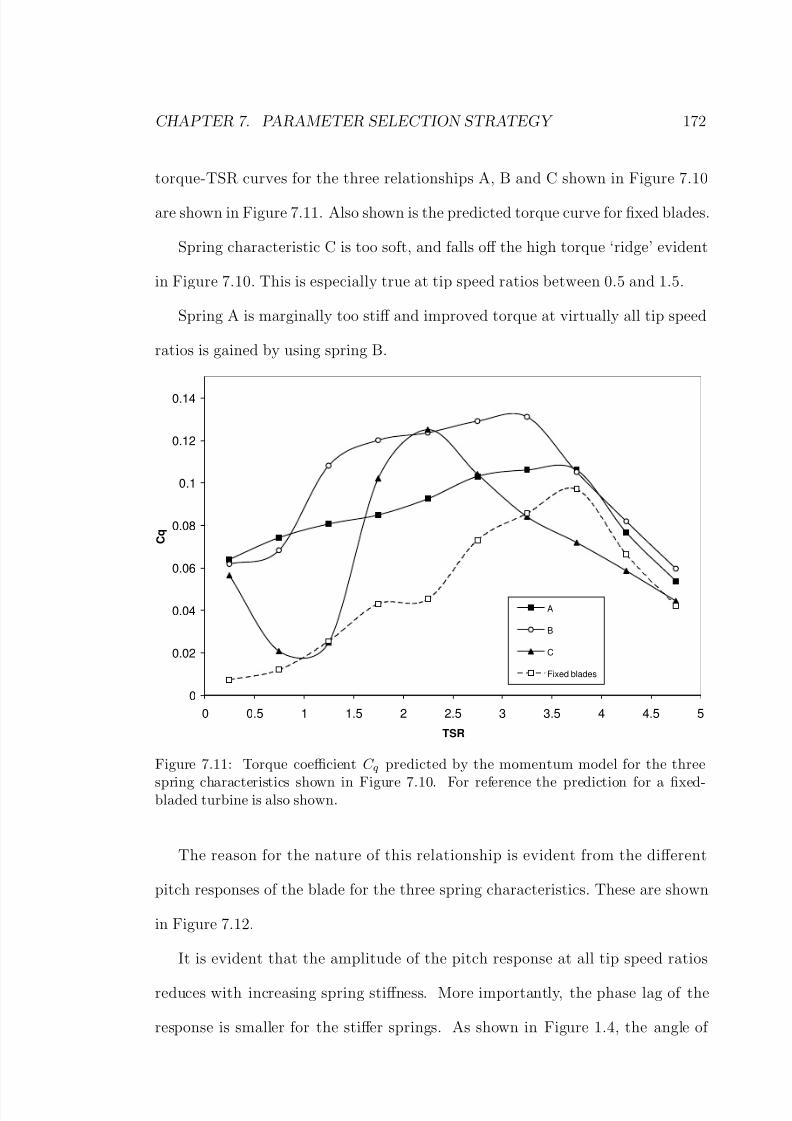
8/13/2019 Wholewhole
http://slidepdf.com/reader/full/wholewhole 197/396
CHAPTER 7. PARAMETER SELECTION STRATEGY 172
torque-TSR curves for the three relationships A, B and C shown in Figure 7.10
are shown in Figure 7.11. Also shown is the predicted torque curve for fixed blades.
Spring characteristic C is too soft, and falls off the high torque ‘ridge’ evident
in Figure 7.10. This is especially true at tip speed ratios between 0.5 and 1.5.
Spring A is marginally too stiff and improved torque at virtually all tip speed
ratios is gained by using spring B.
0
0.02
0.04
0.06
0.08
0.1
0.12
0.14
0 0.5 1 1.5 2 2.5 3 3.5 4 4.5 5
TSR
C q
A
B
C
Fixed blades
Figure 7.11: Torque coefficient C q predicted by the momentum model for the three
spring characteristics shown in Figure 7.10. For reference the prediction for a fixed-bladed turbine is also shown.
The reason for the nature of this relationship is evident from the different
pitch responses of the blade for the three spring characteristics. These are shown
in Figure 7.12.
It is evident that the amplitude of the pitch response at all tip speed ratios
reduces with increasing spring stiffness. More importantly, the phase lag of the
response is smaller for the stiffer springs. As shown in Figure 1.4, the angle of

8/13/2019 Wholewhole
http://slidepdf.com/reader/full/wholewhole 198/396

8/13/2019 Wholewhole
http://slidepdf.com/reader/full/wholewhole 199/396
CHAPTER 7. PARAMETER SELECTION STRATEGY 174
attack variation that drives the pitch response is approximately a sinusoid with
zero crossings at azimuth angles 90 and 270. The pitch response to this variation
should be as close to being in phase as possible. The predicted response for Spring
C, which is the softest spring, shows that for TSR less than one, the pitch angle
is still significantly positive at azimuth 270. This causes the angle of attack on
the blade to be temporarily negative, resulting in severe negative thrust and thus
negative torque.The stiffer springs A and B show a smaller phase lag and correspondingly
better torque at low TSR in Figure 7.11. At the lowest TSR tested of 0.2, all three
springs produce similar torque. This is because at this low speed the blade swings
from one limit to the other (here set to ±40). The limits effectively supplement
the springs and prevent the blade from ever becoming too far out of phase.
As discussed in Section 7.2.3, insight into the pitch response can be gained
by regarding the blade as a single degree of freedom spring/mass/damper system.
The small angle natural frequency for constant rotor speed is (see for example
Thomson (1993)):
ωn =
K
I (7.2)
K is the spring stiffness, I is the mass moment of inertia of the blade assembly.
The damped natural frequency is given by:
ωd =
K
I
−
b
2I
2
(7.3)
where b is the damping coefficient.

8/13/2019 Wholewhole
http://slidepdf.com/reader/full/wholewhole 200/396
CHAPTER 7. PARAMETER SELECTION STRATEGY 175
The response to a harmonic excitation force of frequency ω of such a system is
of the form:
θ = X sin(ωt − β ) (7.4)
The response phase angle β for such a system for a harmonic driving force is given
by:
tan β = b ω
K − Iω2 (7.5)
The amplitude of response to a harmonic excitation is given by:
X = M
(K − Iω2)2 + (b ω)2(7.6)
where M is the amplitude of the harmonic driving moment. The amplitude may
be expressed in terms of the natural frequency ratio ωωn
and damping ratio ζ :
X = M
(1 − ( ωωn
)2)2 + (2ζ ( ωωn
))2(7.7)
These relations are illustrated in Figure 7.13.
If K = amRω2 is proportional to the square of turbine speed as it is in this
case, with small blade damping, the frequency ratio (of turbine speed to natural
frequency) is virtually constant for all but very low speeds.
ω
ωd
≈ω
ωn
= ω
I
K = ω
I
amRω2 =
I
amR (7.8)
Recall that a is a constant defining the spring stiffness. Also note that in the
discussion of natural frequency the notation ω = φ has been adopted for the
turbine speed.

8/13/2019 Wholewhole
http://slidepdf.com/reader/full/wholewhole 201/396
CHAPTER 7. PARAMETER SELECTION STRATEGY 176
Figure 7.13: Non-dimensionalised response amplitude and phase angle for harmonic
excitation for a single degree of freedom spring/mass/damper system. Reproduced fromThomson, W., Theory of Vibration with Applications , 4th ed. Chapman & Hall, 1993.
Figure 7.14 shows that Spring C is closest to the damped natural frequency
at speeds above TSR = 0.5 in this case. The torque coefficient results shown in
Figure 7.10 are plotted again in terms of the damped natural frequency. It is clear
from this plot that maximisation of torque at all tip speed ratios is achieved by a
constant frequency ratio of approximately 0.82 in this case.
The relationship between frequency ratio and the theoretical phase angle for the
spring/mass/damper system is shown in Figure 7.15. Since the damping coefficient
is constant, the damping ratio decreases as turbine speed increases. The phase
angle therefore is greatest at low speeds. The response lags the driving force by
π/2 radians at resonance (frequency ratio of 1), and the proximity to the natural
frequency produces large phase angles even at TSR = 4.

8/13/2019 Wholewhole
http://slidepdf.com/reader/full/wholewhole 202/396
CHAPTER 7. PARAMETER SELECTION STRATEGY 177
While the stiffest spring, A, puts the blade furthest from the natural frequency
and thus produces the smallest phase angle, the reduced amplitude of response at
this frequency ratio is detrimental. At low and intermediate tip speed ratios, the
natural variation in relative wind direction requires a large pitching amplitude to
produce useful torque. If the pitch amplitude is too small, little improvement over
a fixed-blade turbine is gained.
In summary, it is desirable to minimise the natural frequency ratio in orderto minimise the phase angle between aerodynamic driving moment and the pitch
response. If the blade operates too close to or above its natural frequency, the
pitch response lags the wind incidence variation by so much that the sense of
the lift produced is opposite to that needed and severe negative torque results.
A frequency ratio of one is a ‘hard boundary’ beyond which torque drops very
rapidly to negative values.
It is also in general desirable to maximise the pitch response amplitude. For
intermediate tip speed ratios, at which improved performance is the primary focus
of this work, output is generally improved by maximising the pitch amplitude,
so long as the phase angle remains small. A large pitch response reduces the
amplitude of the variation in angle of attack experienced by the blade, which
reduces the proportion of time spent in blade stall. If the pitch response amplitude
is too small, the performance of the turbine approaches that of a fixed bladed
turbine. The region of excessively low frequency ratio constitutes a ‘soft boundary’,
as performance is gradually diminished.
A balance must therefore be struck between an adequately large pitch am-
plitude and an adequately small phase angle. This compromise is assisted by
maximising the aerodynamic driving moment and minimising the blade inertia.

8/13/2019 Wholewhole
http://slidepdf.com/reader/full/wholewhole 203/396
CHAPTER 7. PARAMETER SELECTION STRATEGY 178
For example, if Rac could somehow be increased without changing I , the response
amplitude could be increased without increasing the frequency ratio and so the
phase lag. The desirability of finding blade materials and a design that minimise
mass and moment of inertia is clear. For whatever mass properties are given, Rac
and the inertial or the elastic stiffness may be adjusted to produce a natural fre-
quency ratio that represents an appropriate balance between amplitude and phase.
0
0.25
0.5
0.75
1
1.25
1.5
1.75
2
0 1 2 3 4 5
TSR
F r e q u e n c y R a t i o
ω / ω
ω / ω
ω / ω
ω / ω d
A
B
C
Cq
Figure 7.14: Spring/mass/damper frequency ratio for the three spring characteristics
A,B and C. The torque coefficient is shown by colour as a function of the frequencyratio.

8/13/2019 Wholewhole
http://slidepdf.com/reader/full/wholewhole 204/396
CHAPTER 7. PARAMETER SELECTION STRATEGY 179
0
0.2
0.4
0.6
0.8
1
1.2
1.4
1.6
0 1 2 3 4
TSR
P i t c h
R e p s o n s e P h a s e L a g
[ r a d ]
A
B
C
Figure 7.15: Spring/mass/damper theoretical harmonic excitation response phase anglefor the three spring characteristics A,B and C.
7.3.2 Selection of aerodynamic moment arm Rac
The foregoing analysis was conducted with the aerodynamic moment arm Rac set
at 25 mm. Rac is the distance from the pivot axis to the aerodynamic centre.
Assuming that the driving aerodynamic moment is predominantly provided by
the lift force, the moment is given by:
M aero ∝1
2 ρ c L C L W 2Rac (7.9)
where ρ is the air density, c is the blade chord, L is the blade length, C L is the lift
coefficient and W is the relative flow velocity.
For a given blade and counterweight the mass moment of inertia of the blade
assembly, I , is a function of Rac. I may be estimated by Equation 3.7:
I = I blade + I cw + mtotal
mcw
(mblade(Rac − 0.25c + xcgblade)2 + mtotalR
2
cg)

8/13/2019 Wholewhole
http://slidepdf.com/reader/full/wholewhole 205/396
CHAPTER 7. PARAMETER SELECTION STRATEGY 180
From Equation7.6, the response amplitude is proportional to:
X ∝1
2 ρ c L C L W 2Rac
(K − Iω2)2 + (b ω)2(7.10)
So for a given blade, increasing the aerodynamic moment arm Rac linearly
increases the strength of the aerodynamic driving moment, but also increases the
polar moment of inertia according to Equation 3.7. As Rac approaches zero, M aero
approaches zero but the moment of inertia approaches a finite minimum. The
response amplitude therefore approaches zero. As Rac goes to infinity, I becomes
almost proportional to Rac according to Equation 3.7. The response amplitude
therefore again approaches zero. At some intermediate value of Rac, the ratio
Rac : I is a maximum. Using Equation 3.7 this value, labelled R ∗
ac, is found to be
R ∗
ac =
mcw
mtotal
(I blade + I cw) + (mblade(−0.25c + xcgblade)2 + mtotalR2
cg)
mblade
(7.11)
If damping is zero, the response amplitude for a spring/mass/damper system given
by Equation 7.6 is a maximum at R ∗
ac. For non-zero blade damping, the amplitude
is reduced and the value of Rac giving maximum amplitude increases. For small
damping ratios the ratio Rac
: I gives a good indication of the response amplitude.
Figure 7.16 shows the pitch response amplitude over a range of tip speed ratios
predicted by the momentum model for values of Rac between 25 mm and 200 mm.
Also plotted is the variation of the ratio Rac : I with Rac. The value of R ∗
ac given
by Equation 7.11 is 100 mm in this case, which is the location of the peak Rac : I
value. The variation pitch response amplitude at each tip speed ratio mirrors the
variation in Rac : I . The elastic restoring stiffness is adjusted for each value of Rac
to maintain the same frequency ratio.

8/13/2019 Wholewhole
http://slidepdf.com/reader/full/wholewhole 206/396
CHAPTER 7. PARAMETER SELECTION STRATEGY 181
0
2
4
6
8
10
12
14
16
18
20
0 20 40 60 80 100 120 140 160 180 200
Rac [mm]
P i t c h A m p l i t u d e [ d e g ]
0
2
4
6
8
10
12
14
16
18
R a c
/ I
1.5
2
2.5
3
3.5
4
4.5
5
Rac/I
TSR
Figure 7.16: Pitch response amplitudes predicted by the momentum model for values of
Rac between 25 mm and 200 mm. The elastic restoring moment is adjusted to maintainthe frequency ratio at 0.82 in each case. The variation of the ratio Rac : I with Rac is
also plotted.
Figure 7.17 shows the variation in the stiffness of the restoring spring that
is required to maintain the frequency ratio at a value of 0.822 for the turbine
parameters given in Table 7.1. For any value of Rac, the spring stiffness is assumed
to be proportional to the square of the turbine speed.
Figure 7.18 shows the performance predicted by the momentum model for the
turbine with Rac varied between 25 mm and 200 mm and the spring stiffness
varied as shown in Figure 7.17. For all cases the frequency ratio is the same. The
variation in performance reflects the variation in response amplitudes, as shown in
Figure 7.16, as well as variation in damping ratio, which affects the phase angle.
In general, the larger pitch amplitudes produce improved performance at lower
tip speed ratios, but degrade higher speed performance. The value of Rac chosen
for the analysis shown in Figure 7.10 of 25 mm produces a smaller amplitude

8/13/2019 Wholewhole
http://slidepdf.com/reader/full/wholewhole 207/396
CHAPTER 7. PARAMETER SELECTION STRATEGY 182
0
500
1000
1500
2000
2500
3000
3500
0 1 2 3 4 5
TSR
R e s t o r i n g s p r i n g s t i f f n e s s ,
K [ N m / r a d ]
25
50
75
100
125
150
175
200
Rac [mm]
Figure 7.17: Variation in stiffness of the ‘ideal restoring spring’ required to keep thefrequency ratio constant for a range of values of Rac.
0
0.02
0.04
0.06
0.08
0.1
0.12
0.14
0 0.5 1 1.5 2 2.5 3 3.5 4 4.5 5
TSR
T o r q u e c o e f f i c i e n t , C q
25
5075
100
125
150
175
200
Rac [mm]
Figure 7.18: Torque coefficients predicted by the momentum model for a range of values
of Rac with the elastic restoring moment adjusted as shown in Figure 7.17 to keep thefrequency ratio constant.

8/13/2019 Wholewhole
http://slidepdf.com/reader/full/wholewhole 208/396
CHAPTER 7. PARAMETER SELECTION STRATEGY 183
than would be produced by larger values of Rac. In this case, improved overall
performance results. The value chosen for a particular turbine would depend on
its specific combination of parameters, such as the blade and counterweight mass
and moment of inertia, blade centre of gravity location, aerofoil profile and chord
length and so on.
A large Rac makes the driving aerodynamic moment large relative to the re-
sistance of friction and damping. However there are a number of constraints thatlimit the value of Rac. For a large Rac, the pitching motion of the blade results
in significant translatory motion of the aerodynamic centre. The angle of attack
experienced by the blade is then modified by its own motion. This increases the
aerodynamic damping on the blade that arises from its positive lift curve slope
(this phenomenon is discussed further in Section 7.3.3).
Secondly, a large Rac also places the pivot axis a long way forward, outside
the blade profile. This presents problems from a design point of view. The blade
connection components are then not concealed within the blade and require fairing
to reduce parasitic drag. Further, the large moment arm at which the counter-
weight acts results in large bending loads on the member on which the weight is
mounted. It is likely that such structural considerations would take precedence
over aerodynamic optimisation in most cases.
7.3.3 Blade damping
The current analysis suggests that deliberate damping of the blade motion is not
desirable. Damping serves to reduce the amplitude of the pitch response as well
as increasing the phase lag. If the amplitude is too great, then in general it would
be better to reduce it by reducing the aerodynamic centre moment arm, Rac, to
reduce the driving moment, rather than to add damping. This does not affect
8/13/2019 Wholewhole
http://slidepdf.com/reader/full/wholewhole 209/396
CHAPTER 7. PARAMETER SELECTION STRATEGY 184
the phase of the response and results in a reduced mass moment of inertia for the
blade assembly.
Kirke (1998) stated that the blades on his demonstration turbine were heavy
enough to require damping, by means of damping cylinders that were also used to
limit the blade travel.
Even if some form of damping is not included deliberately, it is assumed that
some damping of the blade pitch motion will arise naturally. Such damping wouldexist within the blade connection itself and as aerodynamic damping.
Hansen (1995) concluded that aerodynamic damping on horizontal axis wind
turbine blades arises primarily from the positive lift-curve slope of the aerofoil. If
the blade ‘flaps’ normal to the rotor plane in the upwind direction, the blade’s
own velocity increases the angle of attack, resulting in increased lift that opposes
the flap motion. Conversely, if the blade moves downwind, the angle of attack
is decreased, resulting in a loss of lift. This effect is inherently related to the
transverse velocity and produces positive damping of blade flap motion. This
damping is not related to viscosity of the air and arises in a potential flow analysis.
It is dependent on the fact that lift is proportional to angle of attack. If the blade
is operating near its stall angle, the negative slope of the lift curve beyond stall
can result in ‘negative damping’, which produces instability.
Aerodynamic damping of this form should emerge naturally from the calcula-
tion of aerodynamic loads so long as the angle of attack takes into account the
motion of the blade. This damping does not need to be included in the damping
coefficient.
Aerodynamic damping arising from the viscosity of the air would need to be
accounted for in the damping coefficient, but this effect is likely to be small. Fung

8/13/2019 Wholewhole
http://slidepdf.com/reader/full/wholewhole 210/396
CHAPTER 7. PARAMETER SELECTION STRATEGY 185
(1955) does not include a separate viscous aerodynamic damping term of this form
in his text on the theory of aeroelasticity.
The value of the damping coefficient is therefore determined mainly from the
structural damping of the blade connection. This damping may well not be viscous,
but instead may be structural (force proportional to displacement). According to
Cook (1995), structural damping is difficult to model mathematically, and it may
be idealised as viscous damping so long as it is small (< 10%).The amount of structural damping that exists would depend on the exact design of the blade
connection. For an elastic type system, especially one using an elastomeric mate-
rial, the damping may be significant. However for a purely inertial system where
nominally no deformation of material is involved, damping would seem to be very
low.
Bayly (1981) included a damping term in his analysis, though did not comment
on its physical origin. He found that the predicted blade pitch pattern would
not converge for critical damping ratios less than 0.1. He tested damping ratios
between 0.1 and 2, and concluded that the value of the damping ratio does not
have a strong influence on performance at tip speed ratios greater than 3.5 (this
was the lower limit of his range of study). It seems logical that the influence of
damping should decrease with increasing tip speed ratio, as the amplitude of the
pitch response naturally decreases with speed.
Kirke (1998) and Lazauskas (1992) make no mention of a damping term in
their mathematical model.
It was found that the value of the damping constant may have a significant
effect on predicted blade pitch response patterns and on the average torque for
the revolution, especially at low and intermediate tip speeds. Increased damping

8/13/2019 Wholewhole
http://slidepdf.com/reader/full/wholewhole 211/396
CHAPTER 7. PARAMETER SELECTION STRATEGY 186
alters the frequency ratio, decreasing the amplitude and increasing the phase angle
of the response.
Damping also accelerates convergence of the pitch response to the steady state
pattern. It was found that instead of converging to a single steady state pitch
response, the blade often settled into a two-revolution period cycle, with the
revolution-average torque alternating between two distinct values. Less commonly,
a three revolution cycle may develop. When this occurred, the check for steady-state convergence would fail, as this was based solely on comparing the torque
coefficient values for the two most recent revolutions.
Increased damping reduces the tendency for multiple-revolution cycles to de-
velop, but also significantly changes the predicted pitch pattern and average torque
(see Figure 7.19). It may also be noted that the general trend is for the torque to
decrease with increasing damping.
For the purposes of these analyses, the damping coefficient has been set to
the lowest value possible that allows convergence to a single torque to occur at
most tip speed ratios. Where a two-revolution pattern persists, an average of
the alternating torque values is taken. This value approximates the steady-state
average torque that would be produced by a turbine with such a two-revolution
period.
It is not clear whether multiple-revolution pitch cycles occur in reality. In the
field, even if the actual damping were low enough for such patterns to develop, it
is likely that continual changes in conditions would not allow precise repetition of
any pattern, whether it had a period of one or two revolutions.

8/13/2019 Wholewhole
http://slidepdf.com/reader/full/wholewhole 212/396
CHAPTER 7. PARAMETER SELECTION STRATEGY 187
0
0.02
0.04
0.06
0.08
0.1
0.12
0.14
0.16
1 2 3 4 5 6 7 8 9 10 11 12 13 14 15 16 17 18 19 20
Revolution
C q
10
5
4
3
2
1
0
TSR 1.75
Damping
coefficient
[Nm/rad/s]
Figure 7.19: Comparison of the convergence of predicted torque coefficient Cq withsuccessive revolutions for different blade damping coefficients.
7.4 Validity of the Spring/Mass/Damper Analogy
The analogy of a mass/spring/damper system response to harmonic forcing is
clearly a simplification of the real situation. Specifically, the aerodynamic forces
and moments that drive blade pitching do not vary in a simple sinusoidal fashion,
especially for TSR< 1 and around blade stall. Aerodynamic forces on the blade
always cause it to seek zero angle of attack. As the amplitude of the pitch response
increases, the angle of attack experienced by the blade tends to zero and so does the
lift force that causes the pitching. If the inertia of the blade causes it to overshoot,
the angle of attack will switch sign and begin to reduce the pitch angle. The pitch
response amplitude is therefore limited by the amplitude of the variation in angle
of attack that would be experienced by a fixed blade at that tip speed ratio. The

8/13/2019 Wholewhole
http://slidepdf.com/reader/full/wholewhole 213/396
CHAPTER 7. PARAMETER SELECTION STRATEGY 188
harmonic forcing spring/mass/damper analogy also breaks down as this point is
approached.
However the analogy is a useful starting point in the design of passive variable-
pitch turbines for which the restoring moment is roughly proportional to the blade
pitch angle.
There are designs for which this approximation is not applicable. The stabiliser
mass concept used in the designs of Liljegren (1984) and Kirke and Lazauskas(1991) produce a restoring moment that is constant in magnitude at a given turbine
speed and is independent of the pitch angle. It is difficult to predict the behaviour
of such a system based on the replacement of the stabiliser mass with a spring. At
best, the stabiliser mass restoring moment could be taken as a kind of average of
a torsion spring moment taken over the pitch amplitude. However the stabiliser
mass moment at pitch angles close to zero is very much greater than would be
applied by the spring and conversely, the mass moment at the extremes of pitch
would be less than the spring moment.
In Section 3.3.4 the concept of tailoring the shape of the rolling profile was ex-
plained. The shape of the profile may be designed so that the relationship between
pitch angle and restoring moment is not linear. In terms of the present analogy
this is akin to providing a torsion spring with a non-linear stiffness characteristic.
If the slope of the moment-angle curve is made to decrease with increasing pitch
angle, then the blade should feel an effectively stiffer spring when its pitch ampli-
tude is small than when the amplitude is large. Theoretically this should enable
the performance of the turbine to be improved, by effectively blending a relatively
‘soft spring’ at low tip speed ratios, where the pitch amplitude is large, with a
‘hard spring’ at high tip speed ratios where the amplitude is small.

8/13/2019 Wholewhole
http://slidepdf.com/reader/full/wholewhole 214/396
CHAPTER 7. PARAMETER SELECTION STRATEGY 189
In some respects the mass stabiliser concept is an extension of this idea. The
‘average’ stiffness of the torsion ‘spring’ felt by the blade depends on the amplitude
of the pitch response. At small amplitudes the mass acts like a very stiff spring,
while at large amplitudes it is more like a soft spring (see Figure 7.20).
Pitch
M o m e n
t
Stabiliser massmoment
Linear springwith sameaverage momentas stabiliser massfor large amplitude
Linear springwith sameaverage momentas stabiliser massfor small amplitude
Figure 7.20: Stabiliser mass torsion spring analogy
For this reason, the stabiliser mass concept is able to allow large pitch ampli-
tudes at low speeds to provide good starting torque, while effectively locking the
blade to zero pitch at high speeds, so the turbine acts like a standard Darrieus.
There is a threshold of restoring moment that has to be overcome in order to
move from zero pitch prevents small oscillations. While this is a desirable trend,
the variation in effective stiffness with pitch amplitude in some instances may be
excessive. Kirke (1998) states in his conclusion that a large pitch amplitude, up
to 45, is an advantage at low tip speed ratios, but that mathematical modelling
indicated that a higher maximum efficiency (attained at high tip speed ratios) was
produced by a smaller pitch amplitude (typically less than 10). It is possible that
8/13/2019 Wholewhole
http://slidepdf.com/reader/full/wholewhole 215/396
CHAPTER 7. PARAMETER SELECTION STRATEGY 190
the limiting of blade pitch to relatively small angles (using stops) was found to be
advantageous because the stops supplemented the stabiliser mass at intermediate
tip speed ratios, preventing the blade motion from becoming too far out of phase
with the wind.
7.5 Summary
Most of the passive variable-pitch design concepts discussed in Chapters 2 and 3
are able to be approximated by a simple mass/spring/damper. The mass stabiliser
designs of Lilegren and Kirke are difficult to characterise in this way because the
restoring moment is constant and not proportional to the pitch angle.
The following conclusions have been reached on the basis of this analysis:
• The magnitude of the restoring moment should be approximately
proportional to the square of the rotor speed. For small damping, this
makes the natural frequency of the blade almost proportional to speed and
the frequency ratio almost constant. Inertial-type designs naturally produce
such a moment.
• The ‘stiffness’ of the restoring moment should be chosen so that
the frequency ratio is less than one. This prevents the blade motion
from being completely out of phase with the driving aerodynamic moment.
• The frequency ratio must be high enough to produce an adequate
pitch response amplitude, but low enough to keep the phase angle
of the response small. If the frequency ratio is too near one, the pitch
response approaches 90. If the frequency ratio is too low, the blade does
not pitch sufficiently and no great improvement over a fixed-bladed turbine

8/13/2019 Wholewhole
http://slidepdf.com/reader/full/wholewhole 216/396
CHAPTER 7. PARAMETER SELECTION STRATEGY 191
is obtained. The exact value depends on the specific turbine parameters and
the degree of damping in the blade mechanism.
• There is a value of the aerodynamic moment arm Rac for which the
ratio Rac : I is a maximum. This value should yield the greatest amplitude
of pitch response and should allow the use of the lowest frequency ratio. A
smaller value may however yield better overall performance, especially at
higher tip speed ratios. It is likely that structural design considerationswould override aerodynamic optimisation in the selection of Rac.
• The above conclusions, based on the modelling of each blade as a
spring/mass/damper system, provide starting points for more de-
tailed analysis using a mathematical model such as the momentum
model. The complexity of Darrieus turbine aerodynamics makes the design
process difficult. The analogy is especially tenuous at tip speed ratios less
than one. Also specific design concepts such as the mass stabiliser design are
not readily treated in this manner.
8/13/2019 Wholewhole
http://slidepdf.com/reader/full/wholewhole 217/396
Chapter 8
Analysis of Turbulent Wind Performance
8.1 Introduction
One of the advantages of the free vortex wake mathematical model over the mo-
mentum model is its ability to handle unsteady conditions. While the self-starting
ability of passive variable-pitch turbines in steady wind has been the focus of this
thesis, the performance of this type of turbine in a turbulent wind has also been
studied.
Both Bayly (1981) and Kirke (1998) identified unsteady wind and its effect on
blade pitch response as an area requiring further study.
8.2 Performance in a Wind of Varying Velocity
Simulation runs using the vortex model were conducted for a turbine operating in
a free wind of fixed direction but sinusoidally varying velocity.
Nattuvetty and Gunkel (1982) performed an analysis of the performance of a
cycloturbine in varying wind. The pattern of pitch variation is predetermined for
the cycloturbine and is independent of tip speed ratio. The present analysis takes
into account the gradual change in pitch response that occurs with changing wind
conditions.
Since the power of the wind is a function of the cube of the wind speed, more
energy passes through a fixed area in one period of a wind of sinusoidally varying
192

8/13/2019 Wholewhole
http://slidepdf.com/reader/full/wholewhole 218/396

8/13/2019 Wholewhole
http://slidepdf.com/reader/full/wholewhole 219/396
CHAPTER 8. ANALYSIS OF TURBULENT WIND PERFORMANCE 194
ratio and power coefficient regardless of wind speed. Such a load arises for example
from the direct heating of water by an impeller attached to the turbine shaft
(Nattuvetty and Gunkel, 1982). The magnitude of the load was chosen so that the
steady-state operating point lies at close to the peak of the power coefficient - tip
speed ratio curve. The steady-state efficiency was found using the vortex model
by performing a simulation run with a constant wind speed of 7 m/s.
Several runs were then conducted using the vortex model with a sinusoidallyvarying wind. From Equation 8.3 the values U = 6.93 m/s, U = 0.99 m/s
were found to give the same average power as a steady wind of 7 m/s, regardless
of the period. The period of oscillation was varied between 2 and 50 seconds.
The resulting oscillation of power transmitted to the load with time is shown in
Figure 8.1. Since the load torque is proportional the square of the speed, the load
power is proportional to the cube of the speed. The speed oscillates at the same
frequency as the wind speed variation. Due to the inertia of the turbine and its
load, the turbine speed lags the wind speed and as the frequency increases, the
amplitude of the turbine speed oscillation diminishes, as the turbine is not able to
respond to the rapid fluctuations.
Nattuvetty and Gunkel (1982) found that for a cycloturbine connected to a
load of this type, all the operating points predicted by his analysis lay on a cubic
curve on the power coefficient-tip speed ratio plot. This fact results from the use
of the load torque to define the power coefficient. Under unsteady conditions, part
of the total torque developed by the turbine drives the load while the remainder
accelerates the inertia of the turbine and load. Because of this the total instanta-
neous power is different from the load power. In examining the self-starting ability
of turbines, the total power was used because both the energy being fed to the load

8/13/2019 Wholewhole
http://slidepdf.com/reader/full/wholewhole 220/396
CHAPTER 8. ANALYSIS OF TURBULENT WIND PERFORMANCE 195
and being used to accelerate the turbine were considered as useful. In the case of a
statistically stationary varying wind, any work done in changing the turbine speed
may be considered as lost. The use of the load power does produce apparently non-
sensical instantaneous power coefficients greater than the steady-state optimum in
a fluctuating wind. This occurs when the turbine speed lags a drop in wind speed
due to inertia and is temporarily driving the load faster than is sustainable. The
turbine soon decelerates however and then lags the wind speed when it rises again,resulting in a lower than optimum power coefficient. The turbine is never allowed
to settle to steady-state and the average power delivered to the load is less than
would be extracted from a steady wind of the same average power.
Rosen and Sheinman (1994) performed a simulation of a horizontal axis wind
turbine in a sinusoidally varying wind. They found that for low frequency vari-
ation the average power coefficient was not significantly lower than for a steady
wind. However as the frequency increased, the effect on efficiency become more
pronounced. There was a frequency at which the deviation from steady wind
performance was greatest and for higher frequencies, the performance recovered
towards the steady wind level. This was explained as the turbine’s inability to
respond to such rapid variations in the wind. A similar trend was observed with
the present results, shown in Table 8.2.
Results for two different total (turbine and load) mass moments of inertia (I t)
are presented. The lower inertia is for a turbine with a bare rotor plus load moment
of inertia of 100 kgm2, resulting in a total moment of inertia of 866 kgm2. The
heavier rotor has a mass moment of inertia of 1000 kgm2, giving a total inertia of
1766 kgm2. The remainder of the inertia comes from the blades.
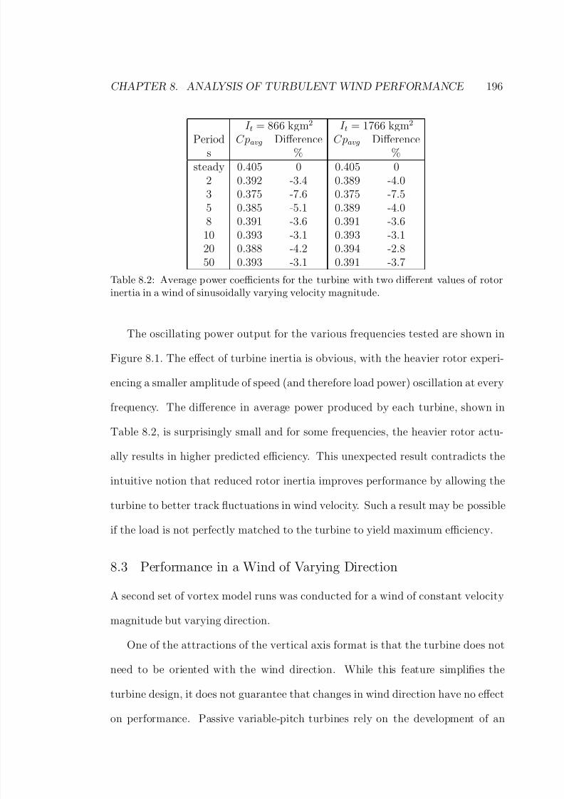
8/13/2019 Wholewhole
http://slidepdf.com/reader/full/wholewhole 221/396
CHAPTER 8. ANALYSIS OF TURBULENT WIND PERFORMANCE 196
I t = 866 kgm2 I t = 1766 kgm2
Period Cpavg Difference Cpavg Differences % %
steady 0.405 0 0.405 02 0.392 -3.4 0.389 -4.03 0.375 -7.6 0.375 -7.55 0.385 -5.1 0.389 -4.08 0.391 -3.6 0.391 -3.6
10 0.393 -3.1 0.393 -3.120 0.388 -4.2 0.394 -2.850 0.393 -3.1 0.391 -3.7
Table 8.2: Average power coefficients for the turbine with two different values of rotorinertia in a wind of sinusoidally varying velocity magnitude.
The oscillating power output for the various frequencies tested are shown in
Figure 8.1. The effect of turbine inertia is obvious, with the heavier rotor experi-
encing a smaller amplitude of speed (and therefore load power) oscillation at every
frequency. The difference in average power produced by each turbine, shown in
Table 8.2, is surprisingly small and for some frequencies, the heavier rotor actu-
ally results in higher predicted efficiency. This unexpected result contradicts the
intuitive notion that reduced rotor inertia improves performance by allowing the
turbine to better track fluctuations in wind velocity. Such a result may be possible
if the load is not perfectly matched to the turbine to yield maximum efficiency.
8.3 Performance in a Wind of Varying Direction
A second set of vortex model runs was conducted for a wind of constant velocity
magnitude but varying direction.
One of the attractions of the vertical axis format is that the turbine does not
need to be oriented with the wind direction. While this feature simplifies the
turbine design, it does not guarantee that changes in wind direction have no effecton performance. Passive variable-pitch turbines rely on the development of an

8/13/2019 Wholewhole
http://slidepdf.com/reader/full/wholewhole 222/396
CHAPTER 8. ANALYSIS OF TURBULENT WIND PERFORMANCE 197
1000
1100
1200
1300
1400
1500
1600
1700
1800
140 150 160 170 180 190 200
Time [s]
P o w e r [ W ]
1000
1100
1200
1300
1400
1500
1600
1700
1800
140 150 160 170 180 190 200
Time [s]
P o w e r [ W ]
I t = 1766 kgm2 I t = 866 kgm2
Figure 8.1: Variation in power at steady-state in winds of fluctuating magnitude for twovalues of turbine mass moment of inertia. The different frequencies of oscillation areevident in the power fluctuations.
appropriate pattern of blade pitch response. This pattern is oriented relative to
the wind direction and takes some time to develop. If the wind direction changes,
the pattern of pitch must change in response and this change takes some finite
time. In the interim, the phase of the pitch response is effectively changed. If the
wind direction is constantly varying, then the steady-state pitch response pattern
may never have a chance to develop, and the efficiency of the turbine may be
diminished.
A turbine with the parameters given in Table 8.1 and with turbine inertia I t
equal to 1766 kgm2 was simulated using the vortex model in a wind of constant
magnitude but varying direction. The wind speed was set at 7 m/s and the direc-
tion varied sinusoidally between limits of ±45. The frequency of the oscillation
was varied between 2 and 20 seconds.
Once the turbine had reached steady-state, the average output power was cal-
culated over an integer number of periods for each case. The results are compared
with the steady-state power for a steady wind in Table 8.3. The trend of the
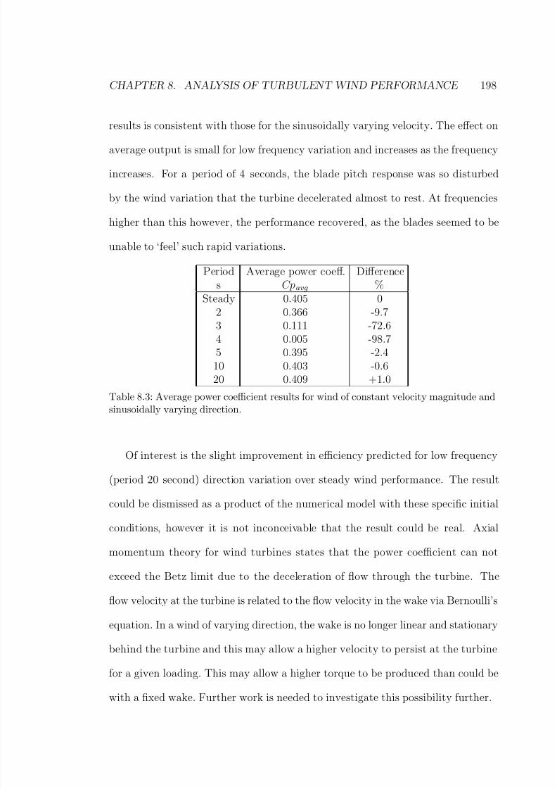
8/13/2019 Wholewhole
http://slidepdf.com/reader/full/wholewhole 223/396
CHAPTER 8. ANALYSIS OF TURBULENT WIND PERFORMANCE 198
results is consistent with those for the sinusoidally varying velocity. The effect on
average output is small for low frequency variation and increases as the frequency
increases. For a period of 4 seconds, the blade pitch response was so disturbed
by the wind variation that the turbine decelerated almost to rest. At frequencies
higher than this however, the performance recovered, as the blades seemed to be
unable to ‘feel’ such rapid variations.
Period Average power coeff. Differences Cpavg %Steady 0.405 0
2 0.366 -9.73 0.111 -72.64 0.005 -98.75 0.395 -2.4
10 0.403 -0.620 0.409 +1.0
Table 8.3: Average power coefficient results for wind of constant velocity magnitude and
sinusoidally varying direction.
Of interest is the slight improvement in efficiency predicted for low frequency
(period 20 second) direction variation over steady wind performance. The result
could be dismissed as a product of the numerical model with these specific initial
conditions, however it is not inconceivable that the result could be real. Axial
momentum theory for wind turbines states that the power coefficient can not
exceed the Betz limit due to the deceleration of flow through the turbine. The
flow velocity at the turbine is related to the flow velocity in the wake via Bernoulli’s
equation. In a wind of varying direction, the wake is no longer linear and stationary
behind the turbine and this may allow a higher velocity to persist at the turbine
for a given loading. This may allow a higher torque to be produced than could be
with a fixed wake. Further work is needed to investigate this possibility further.
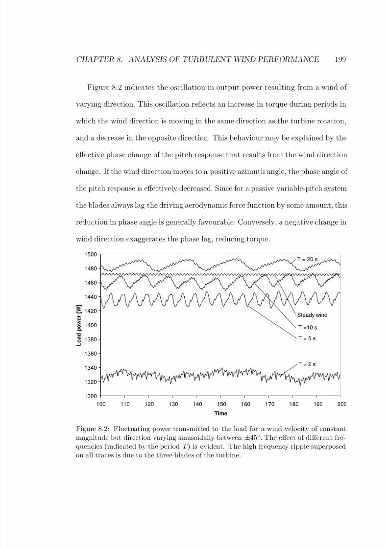
8/13/2019 Wholewhole
http://slidepdf.com/reader/full/wholewhole 224/396

8/13/2019 Wholewhole
http://slidepdf.com/reader/full/wholewhole 225/396

8/13/2019 Wholewhole
http://slidepdf.com/reader/full/wholewhole 226/396
CHAPTER 8. ANALYSIS OF TURBULENT WIND PERFORMANCE 201
-10
-8
-6
-4
-2
0
2
4
6
8
10
0 50 100 150 200 250 300 350 400 450 500
Time [s]
V e l o c i t y [ m / s ]
Longitudinal component
Lateral component
Figure 8.3: Longitudinal and lateral velocity components generated by the Dryden tur-bulence filter.
ratio in the range of interest, then the overall efficiency may actually be greater
than that for the mean steady wind. The opposite is true for a positive Cp-TSR
slope. The work of Rosen and Sheinman (1994) on horizontal axis wind turbines
demonstrates this relationship.
Ideally, the turbine speed should be set so that it operates at close to the peak
of the Cp-TSR curve as possible. In this case, any deviation in wind speed causes
a reduction in power coefficient and so the overall efficiency will be reduced, as
stated by Nattuvetty and Gunkel (1982).
For a turbine that is not constrained to operate at a constant speed, the inertia
of the system becomes important. For a hydraulic type load, where the torque is
proportional to the square of the speed, the turbine should operate at the same
steady-state tip speed ratio, no matter what the wind speed. If it had zero inertia,
the turbine would always be able to operate at this tip speed ratio even in a
turbulent wind and would suffer no loss of efficiency. The slope of the Cp curve

8/13/2019 Wholewhole
http://slidepdf.com/reader/full/wholewhole 227/396

8/13/2019 Wholewhole
http://slidepdf.com/reader/full/wholewhole 228/396
CHAPTER 8. ANALYSIS OF TURBULENT WIND PERFORMANCE 203
Table 8.1. The blade mass moments of inertia (I pivot) were calculated using Equa-
tion 3.7 in Section 3.3.4. It was found that because the Pendulum A turbine
had a greater mass moment of inertia, it had a higher natural frequency ratio
for the same restoring moment. In this case diminished performance resulted, so
the Pendulum B turbine was included with an increased mass centre moment arm
to match the frequency ratio of the other designs. The steady-state performance
predicted for this design closely matched those of the Rolling Profile and Elasticdesigns (see Figure 8.4). It was desired to see whether the higher mass moment of
inertia of the Pendulum designs would affect performance in a turbulent wind.
Parameter Rolling Elastic Pendulum Pendulum Fixedprofile A B blades
Rac / mm 40 40 40 40 40Restoring moment 55a 55b 55c 75c -I pivot / kgm2 3.19d 3.19 3.79 4.30 -
Load torque / (Nm/(rad/s)2
) 3.6 3.6 3.6 3.6 1.5a Distance from centre of curvature to mass centre [mm]bTorsion spring stiffness constant (stiffness proportional to centrifugal load) [(Nmm/rad)/N]cDistance from pivot axis to mass centre [mm]d Mass moment of inertia about the centre of mass
Table 8.5: Parameters of turbines simulated in a “real” wind. All other parameters arethe same as for Table 8.1.
A fixed-bladed (standard Darrieus) turbine was also included in the compar-
ison. The predicted steady state performance is included in Figure 8.4. Because
the shape of the torque speed for the Darrieus turbine is different from that of
the variable-pitch turbines, a different load characteristic was chosen to suit it.
It was found that the operating point had to be located at a slightly higher tip
speed ratio than would yield the greatest steady-state efficiency because the lack
of torque at lower speeds made it difficult to converge to the steady-state. A load
of 1.5 Nm/(rad/s)2 was finally used.

8/13/2019 Wholewhole
http://slidepdf.com/reader/full/wholewhole 229/396
CHAPTER 8. ANALYSIS OF TURBULENT WIND PERFORMANCE 204
0
0.05
0.1
0.15
0.2
0.25
0.3
0.35
0.4
0.45
.
0 0.5 1 1.5 2 2.5 3 3.5 4 4.5 5
TSR
C p
Rolling profile
Pendulum A
Pendulum B
Elastic
Fixed blades
Load 3.6 Nm/(rad/s)^2
Load 1.5 Nm/(rad/s)^2
7 m/s
0
0.02
0.04
0.06
0.08
0.1
0.12
0.14
0 0.5 1 1.5 2 2.5 3 3.5 4 4.5 5
TSR
C q
Rolling profile
Pendulum A
Pendulum B
Elastic
Fixed blades
Load 3.6
Load 1.5
7 m/s
Figure 8.4: Momentum theory steady-state performance curves for the turbines listed
in Table 8.5

8/13/2019 Wholewhole
http://slidepdf.com/reader/full/wholewhole 230/396
CHAPTER 8. ANALYSIS OF TURBULENT WIND PERFORMANCE 205
The load power histories of the turbines over 500 seconds (some 26,000 time
steps) is shown in Figure 8.5. The average power coefficients for the period are
presented in Table 8.6. These values include the integrated load power and the
change in kinetic energy of the turbine calculated from the difference between in
initial and final speed. The runs were started with the turbines at approximately
the steady-state speed for the equivalent steady wind of 7.7 m/s. This speed yields
the same average power as the turbulent wind series. The average efficiency in theturbulent wind is compared with the steady-state power coefficient at this wind
speed.
It is evident that the average power in a more realistic wind is reduced by a
greater amount than in the simple sinusoidally varying cases. The rolling profile
design is predicted to handle the turbulent wind slightly better than the other
designs. The pendulum designs, with their greater blade inertia, suffered more in
these conditions.
The predicted performance loss for the fixed-bladed Darrieus turbine is consid-
erably greater than for the variable-pitch turbines, despite the fact that it does not
suffer from any lag of blade pitch response. It appears that the sharper drop-off
in torque at intermediate tip speed ratios characteristic of fixed-bladed turbines
significantly affects the average efficiency in a turbulent wind, where sudden gusts
force the turbine to operate for considerable periods in this region. Figure 8.4
shows clearly that while the torque produced by the variable-pitch turbines is
maintained at low tip speed ratios, the Darrieus turbine curve drops sharply be-
low the peak. The difference between the turbine torque and the load torque at
a given tip speed ratio determines the acceleration of the turbine. It is clear that
even for the smaller load (1.5 Nm/(rad/s)2), the gap between turbine and load
8/13/2019 Wholewhole
http://slidepdf.com/reader/full/wholewhole 231/396
CHAPTER 8. ANALYSIS OF TURBULENT WIND PERFORMANCE 206
torque curves below the intersection point is smaller than for the variable-pitch
turbines. This means that when a gust of wind arrives and the tip speed ratio
is momentarily reduced, less torque is available to accelerate the turbine. The
Darrieus turbine is therefore less able to track variations in wind speed.
A simulation run was also conducted for the rolling profile and fixed bladed
turbines with reduced rotor moment of inertia (I t = 866 kgm2 compared with
I t = 1766 kgm
2
as before). In this instance the lower inertia allowed the turbinewith the rolling profile to track the wind velocity more effectively, reducing the
variation in tip speed ratio and resulting in a clear improvement in performance.
This is in line with expectation, unlike the results obtained for the sinusoidally
varying wind speed presented in Section 8.2.
The difference in performance between the two fixed-bladed turbines is smaller
than expected. It appears from Figure 8.6 that during gusts the lighter rotor allows
the turbine to accelerate and extract more power, however this gain is offset by
the deceleration of the rotor during lulls.
These results suggest that the shape of the turbine torque curve is the most
important factor in determining the average efficiency of the turbine in turbulent
conditions. The proportions of time spent at tip speed ratios above and below the
equilibrium is influenced by the shape of the torque curve either side of the steady
operating point.
8.5 Conclusion
Vortex model simulations of a passive variable-pitch VAWT were conducted for
winds of sinusoidally varying magnitude and direction over a range of frequencies.
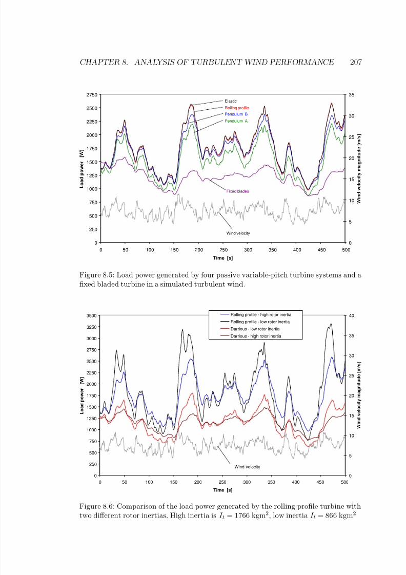
8/13/2019 Wholewhole
http://slidepdf.com/reader/full/wholewhole 232/396
CHAPTER 8. ANALYSIS OF TURBULENT WIND PERFORMANCE 207
0
250
500
750
1000
1250
1500
1750
2000
2250
2500
2750
0 50 100 150 200 250 300 350 400 450 500
Time [s]
L o a d p o w e r
[ W ]
0
5
10
15
20
25
30
35
W
i n d v e l o c i t y m a g n i t u d e [ m / s ]
Wind velocity
Fixed blades
Elastic
Rolling profile
Pendulum B
Pendulum A
Figure 8.5: Load power generated by four passive variable-pitch turbine systems and afixed bladed turbine in a simulated turbulent wind.
0
250
500
750
1000
1250
1500
1750
2000
2250
2500
2750
3000
3250
3500
0 50 100 150 200 250 300 350 400 450 500
Time [s]
L o a d p o w e r
[ W ]
0
5
10
15
20
25
30
35
40
W i n d v e l o c i t y m a g n i t u d e [ m / s ]
Rolling profile - high rotor inertia
Rolling profile - low rotor inertia
Darrieus - low rotor inertia
Darrieus - high rotor inertia
Wind velocity
Figure 8.6: Comparison of the load power generated by the rolling profile turbine withtwo different rotor inertias. High inertia is I t = 1766 kgm2, low inertia I t = 866 kgm2

8/13/2019 Wholewhole
http://slidepdf.com/reader/full/wholewhole 233/396
CHAPTER 8. ANALYSIS OF TURBULENT WIND PERFORMANCE 208
Average power coefficient 7.7 m/s Turbulent Difference
Cpavg steady wind %Rolling profile 0.407 0.364 -10.5Elastic 0.414 0.367 -11.3Pendulum A 0.367 0.321 -12.5Pendulum B 0.405 0.354 -12.5Fixed blades 0.333 0.240 -27.9Rolling profile - low inertia 0.407 0.373 -8.3Fixed blades - low inertia 0.333 0.245 -26.3
Table 8.6: Average power coefficient results for five turbines in a turbulent wind
It was found that the deviation of average output from steady-wind perfor-
mance increased with increasing frequency of variation up to a point, beyond
which the turbine appeared to be unable to respond to such rapid variations.
Simulation of performance in a turbulent wind has indicated the importance of
a ‘flat’ Cp-TSR curve to maximise total energy capture. In the current trial, tur-
bulent wind efficiency was predicted to be 28% lower than steady wind efficiency
for a Darrieus turbine. The corresponding difference for a rolling profile passive
variable-pitch was 10.5%. Variable-pitch mechanisms are therefore not only im-
portant for self-starting, but can also significantly increase the average efficiency
in turbulent conditions. Minimisation of the mass moment of inertia of the turbine
and load appears to be of secondary importance, as does the minimisation of blade
inertia.

8/13/2019 Wholewhole
http://slidepdf.com/reader/full/wholewhole 234/396

8/13/2019 Wholewhole
http://slidepdf.com/reader/full/wholewhole 235/396
CHAPTER 9. EXPERIMENTAL EVALUATION 210
The option of field testing would remove the limitation on size and allow the
turbine to be studied in the conditions in which it would ultimately operate. The
inability to control or even accurately measure the free wind velocity and direc-
tion at the turbine however would make analysis of performance difficult. Only
averaged quantities would be reliably obtained.
The third option of vehicle or trailer-mounted testing offered the possibility of
controlling the wind velocity and direction, if still air conditions occurred. Thereremained the possibility of disturbed flow from the vehicle affecting turbine per-
formance. Also practical considerations would limit the size of the turbine that
could be tested in this fashion. A final major disadvantage was the likelihood that
movement and vibration of the vehicle would significantly affect the pitch response
patterns of the blades. Given the predicted sensitivity of turbine performance to
the blade response pattern, this would be a major problem.
The final issue affecting any form of outdoor testing was that the photogram-
metric pitch measurement method that was developed (which is described in Sec-
tion 9.4.3) relied upon the ability to reduce ambient light. This could only be
achieved in the wind tunnel. Accordingly, the wind tunnel was chosen as the most
appropriate method of testing.
9.2 Prototype Turbine Design
A turbine was built for testing in the large test section of the closed-circuit wind
tunnel at the UNSW. The size of the turbine was determined by the size of the
available wind tunnel test section. As mentioned above, it was desired to make
the turbine as close to a real operational size as possible within the constraints
of the test section area. The smaller the turbine of a given solidity, the smaller
the blade chord and therefore the smaller blade Reynolds number. This results in

8/13/2019 Wholewhole
http://slidepdf.com/reader/full/wholewhole 236/396
CHAPTER 9. EXPERIMENTAL EVALUATION 211
earlier blade stall and reduced starting performance. If the blade chord is made
large relative to the turbine radius to overcome this, the effect of flow curvature is
amplified.
The turbine speed required to achieve a given tip speed ratio at a given wind
speed is inversely proportional to the turbine radius. The centrifugal load on a
blade is therefore inversely proportional to the square of turbine radius. Maximis-
ing the radius at which a blade of given length is mounted therefore reduces thebending loads on it, as well as increasing the swept area and power capacity of the
turbine.
The test section available at UNSW is octagonal in cross section with a height
and width of approximately 3 metres (see Figure 9.1). The turbine dimensions
were chosen to be diameter 1.8 metres and height 1.3 metres, giving a swept area
of 2.34 square metres.
Figure 9.1: Turbine in the 3 metre high wind tunnel test section

8/13/2019 Wholewhole
http://slidepdf.com/reader/full/wholewhole 237/396
CHAPTER 9. EXPERIMENTAL EVALUATION 212
The blade chord was set at 150 millimetres, giving an aspect ratio of 8.67. The
turbine was designed with three blades, giving a solidity of N bc/R = 0.5. This
relatively high solidity was chosen to assist starting performance.
The NACA 0018 profile was chosen as the blade section. This section is com-
monly used for Darrieus turbines. Its relatively high thickness to chord ratio gives
it good strength in bending and its aerodynamic properties are well documented.
The radial arms of the turbine were made from high strength aluminium grade6061-T6. They were NC milled to an Eppler 862 non-lifting profile to reduce
parasitic drag.
9.3 Blade Design
Unlike horizontal-axis turbines, the straight blades of a vertical axis turbine are
loaded in bending by their self-weight under centrifugal force. Horizontal axis tur-
bine blades take centrifugal loads in tension, which produces much lower maximum
stresses. While aerodynamic forces produce bending loads, these are an order of
magnitude lower than inertial loads at design speed.
The blade bending loads are a significant hurdle to be overcome in the design of
a straight-bladed VAWT. The curved troposkien-shaped blades of large Darrieus
turbines are designed to minimise bending loads, but blade articulation is then not
possible.
Often blades designed for this type of turbine are based around a central struc-
tural spar, to which ribs are attached and around which a thin skin is fastened, to
form the desired blade profile. The blade designs described by Bayly (1981) and
Kirke (1998) are of this type.
Since the primary concern is bending stress due to the self-weight of the blades,
the minimisation of mass and maximisation of cross-sectional area moment of

8/13/2019 Wholewhole
http://slidepdf.com/reader/full/wholewhole 238/396
CHAPTER 9. EXPERIMENTAL EVALUATION 213
inertia are paramount. Apart from selecting a material with a high strength-to-
weight ratio, these criteria require that material be located as far from the section
neutral axis (the blade chord line) as possible. For a prismatic blade the ratio
of area moment of inertia of the section to cross-sectional area, I/A, should be
maximised. For this application, a solid section blade is far worse than a hollow
blade, as material near the neutral axis adds mass without contributing much
bending strength. It may be shown that for a given profile with constant wallthickness, the limit of I /A as wall thickness goes to zero is two times that for the
solid section. This principle led to the adoption of a design in which the blade skin
is the structural component, rather than an aerodynamic covering over a structural
skeleton. Clearly design to avoid buckling failure must be done carefully in this
case.
Often blades are constructed so that they are attached to the rotor at two
points. In order to minimise bending stress, the mounting points are located at
some distance in from the ends. For example Evans (1978) calculates that for a
blade of uniform section, the bending moment at midspan and mounting points
is made equal by locating the supports a distance of L/(2 + 2√
2), approximately
0.207L, in from each end. This reduces the maximum bending moment by a factor
of 1/5.8 compared with simply supporting the blades at its ends.
In this case, because the focus of the project was on the design of the blade
mounts, it was felt that it was desirable to have the blade mounted at its ends.
This would allow easiest access to the blade connection area, which would require
frequent adjustment. In addition, it allowed the blade to be mounted without
breaking the skin - an important consideration if the skin is to be used as the
structural member. Finally, it was intended to mount the turbine in the wind

8/13/2019 Wholewhole
http://slidepdf.com/reader/full/wholewhole 239/396
CHAPTER 9. EXPERIMENTAL EVALUATION 214
tunnel using supports connected to the floor and ceiling, making end-mounting of
the blade more desirable.
In order to reduce the bending moment in the middle of the blade, it was de-
cided to utilise counterweights, cantilevered above and below the mounting points.
The counterweights that are needed to balance the blade about its pivot axis can
then serve two purposes. They will act as ‘virtual’ blade length outside the mount-
ing points, playing the same role as the roughly 20% of the uniform section bladecalculated by Evans (1978). This design is shown in Figures 9.2 and 9.3.
Figure 9.2: Blade design featuring cantilevered counterweights
The difficulty with this design is that the cantilevered spar on which the coun-
terweight is mounted is subjected to significant bending and torsional loading. The
spar must be made of a high strength material capable of withstanding these high
loads. In this case high strength stainless steel - Sandvik SAF 2205 - was chosen.
This has a high yield stress (450 MPa) and was selected for its corrosion resistance
so that the turbine could be used for outdoor testing in the future.
An undergraduate thesis completed at UNSW by Dawson (2000) involved a
detailed finite element analysis of different blade designs for this project using
MSC/PATRAN and MSC/NASTRAN. His work indicated that the lowest max-
imum stresses could be obtained using a structural skin with no internal spars
or ribbing. The skin could be aluminium or fibreglass. Dawson performed linear

8/13/2019 Wholewhole
http://slidepdf.com/reader/full/wholewhole 240/396
CHAPTER 9. EXPERIMENTAL EVALUATION 215
Figure 9.3: Detail of blade design concept showing cantilevered counterweight
static analyses to predict maximum Von Mises stress, as well as running buckling
analyses to check for buckling failure.
Further finite element analysis using Pro/FEM was conducted by the author
on the specific design chosen for the prototype turbine that was built for the wind
tunnel. The mesh generated for the blade is shown in Figure 9.4. Symmetry was
exploited to allow modelling of one half of the blade. A ‘gravity’ acceleration of
200 g was applied, corresponding to a rotational speed of approximately 450 rpm
at a radius of 900 mm.
Skin material was chosen as 1.27 mm thick aluminium sheet. Carbon fibre
was investigated as a possible material for blade manufacture, but the cost for
the manufacture of three blades was found to be prohibitive. A relatively high-
strength alloy - 6061-T6 - was chosen, giving a nominal yield stress of 240 MPa.
A counterweight mass was chosen and its chordwise location adjusted so that the

8/13/2019 Wholewhole
http://slidepdf.com/reader/full/wholewhole 241/396
CHAPTER 9. EXPERIMENTAL EVALUATION 216
Figure 9.4: Finite element mesh

8/13/2019 Wholewhole
http://slidepdf.com/reader/full/wholewhole 242/396
CHAPTER 9. EXPERIMENTAL EVALUATION 217
(a)
(b)
Figure 9.5: Colour fringe plot indicating predicted von Mises stress in the blade skin (a)
and the counterweight spar (b)

8/13/2019 Wholewhole
http://slidepdf.com/reader/full/wholewhole 243/396

8/13/2019 Wholewhole
http://slidepdf.com/reader/full/wholewhole 244/396
CHAPTER 9. EXPERIMENTAL EVALUATION 219
Pro/ENGINEER model
Finished assembly
Figure 9.6: Blade end assembly

8/13/2019 Wholewhole
http://slidepdf.com/reader/full/wholewhole 245/396
CHAPTER 9. EXPERIMENTAL EVALUATION 220
(a) Application of glue to blade trailing edge
(b) Blade skin in mould used for clamping while the glue set
Figure 9.7: Construction of the blades

8/13/2019 Wholewhole
http://slidepdf.com/reader/full/wholewhole 246/396
CHAPTER 9. EXPERIMENTAL EVALUATION 221
Figure 9.8: The ‘Type A’ elastomeric blade mounting component on the turbine rig.
inside the wind tunnel test section is shown in Figure 9.9.
9.3.1 Aerodynamic testing of blades
The major concern for the blade design chosen was whether the construction
method would deliver sufficient accuracy in the blade profile from an aerodynamic
standpoint. In order to test the aerodynamic properties of the blades, wind tunnel
testing was performed to measure lift and drag coefficients. The test blade had
the same chord length of 150 mm as the blades used on the turbine, but was cut
shorter to fit inside the 3 x 4 ft (614 x 1218 mm) wind tunnel test section. The
test blade was 1 m long, giving an aspect ratio of 6.67. The blades used on the

8/13/2019 Wholewhole
http://slidepdf.com/reader/full/wholewhole 247/396
CHAPTER 9. EXPERIMENTAL EVALUATION 222
Figure 9.9: The author with the finished rig in the wind tunnel.
turbine were 1300 mm long, with an aspect ratio of 8.67. The test blade is shown
in the test section in Fig. 9.10.
Lift and drag coefficients were measured at wind speeds ranging from 16 m/s
to 36 m/s and at angles of attack from -15 to +50. Forces were measured using
a 6-component pyramidal balance. A calibration was performed with zero wind
velocity to eliminate the effect of the mass of the blade. The results are shown in
Fig. 9.11.
For comparison the data of Sheldahl and Klimas (1981) for the NACA 0018
section are also shown in Figure 9.11. These data were used in the mathematical
models because they provide a complete range of values for all angles of attack and

8/13/2019 Wholewhole
http://slidepdf.com/reader/full/wholewhole 248/396
CHAPTER 9. EXPERIMENTAL EVALUATION 223
Figure 9.10: Test blade mounted in the wind tunnel
over a large range of Reynolds numbers. It can be seen from Figure 9.11 that the lift
and drag coefficients measured here are quite similar to the published values. At all
tested Reynolds numbers, stall occurs at a higher angle of attack and occurs more
suddenly than was measured by Sheldahl and Klimas. Correspondingly higher
maximum lift coefficients were also recorded. As expected, the stall is delayed
with increasing Reynolds number over this range.
The delayed stall may be a result of the manufacturing technique, which does
leave slight artifacts of the forming process. A series of parallel bends are visible
near the leading edge, which may serve to ‘trip’ laminar flow to become turbulent.
There was however little measured increase in drag associated with this effect.
It was concluded on the basis of this testing that the chosen blade design and
manufacturing technique produced blades of sufficient profile accuracy to be used
as turbine blades.
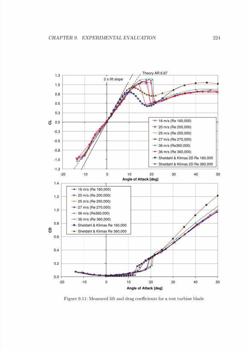
8/13/2019 Wholewhole
http://slidepdf.com/reader/full/wholewhole 249/396
CHAPTER 9. EXPERIMENTAL EVALUATION 224
-1.3
-1.0
-0.8
-0.5
-0.3
0.0
0.3
0.5
0.8
1.0
1.3
-20 -10 0 10 20 30 40 50
Angle of Attack [deg]
C L
16 m/s (Re 160,000)20 m/s (Re 200,000)
25 m/s (Re 250,000)
27 m/s (Re 270,000)
36 m/s (Re360,000)
36 m/s (Re 360,000)
Sheldahl & Klimas 2D Re 160,000
Sheldahl & Klimas 2D Re 360,000
2 π lift slope
Theory AR 6.67
0.0
0.2
0.4
0.6
0.8
1.0
1.2
1.4
-20 -10 0 10 20 30 40 50
Angle of Attack [deg]
C D
16 m/s (Re 160,000)
20 m/s (Re 200,000)
25 m/s (Re 250,000)
27 m/s (Re 270,000)
36 m/s (Re360,000)
36 m/s (Re 360,000)
Sheldahl & Klimas Re 160,000
Sheldahl & Klimas Re 360,000
Figure 9.11: Measured lift and drag coefficients for a test turbine blade

8/13/2019 Wholewhole
http://slidepdf.com/reader/full/wholewhole 250/396
CHAPTER 9. EXPERIMENTAL EVALUATION 225
9.4 Instrumentation
9.4.1 Torque and speed measurement
The quantities measured were the turbine rotational speed and torque. Speed was
measured using a 720 pulse-per-revolution shaft encoder mounted at the top of the
turbine shaft. Torque was measured using a load cell attached to a brake calliper
that acted on a brake disc keyed to the shaft. Commercial panel meters were used
for signal conditioning and digital conversion. The data was logged by a PC, which
was connected to the panel meters via the serial port.
The turbine torque calculated is a combination of shaft torque measured by
the load cell on the brake and torque that is accelerating the turbine. Acceleration
torque was calculated by numerically differentiating the logged turbine speed data.
Because numerical differentiation magnifies the small scatter in the measured speed
values, the acceleration curve was smoothed by fitting a cubic spline through thevelocity data. The data was thinned from the sampling frequency of approximately
3 Hz to a period of 5 seconds, which was judged sufficient to capture the features of
interest in the speed history. The spline was then fitted through the thinned data
points. The slope of the spline at the data points, which is naturally calculated in
the process of fitting the spline, is then used as the acceleration at that time.
Torque is calculated by multiplying acceleration by the polar moment of inertia
of the rotor and blades, calculated using the Pro/ENGINEER model.
The shaft or load torque measured by the load cell connected to the brake
calliper exhibited considerable scatter resulting from slight misalignment between
the disc, shaft and calliper. The fluctuating torque data was smoothed taking a
rolling average.
The total torque produced by the turbine at any point in time was then taken
to be the sum of the acceleration torque and the load torque. The non-dimensional

8/13/2019 Wholewhole
http://slidepdf.com/reader/full/wholewhole 251/396
CHAPTER 9. EXPERIMENTAL EVALUATION 226
torque coefficient, C q, is defined as:
C q = T acc + T load
1
2ρAU 2
∞R
(9.1)
where ρ is the air density, A is the swept area of the turbine, U ∞ is the free wind
velocity and R is the turbine radius.
The torque coefficient calculated in this way reflects the total aerodynamic
torque generated by the turbine at a given speed. If the turbine is at steady-
state, the torque used to accelerate the turbine, T acc is zero, and all the torque
is used to drive the load. At tip speed ratios lower than the steady-state speed,
the turbine will be accelerating and T acc will be non-zero. This means that the
torque coefficient calculated using Equation 9.1 is larger than that calculated using
the load torque alone. In the study of the self-starting ability of turbines, the
transmission of energy to the load is not considered to be the only useful work
being done: the acceleration of the turbine to steady-state operating speed is a
task that otherwise must be done using external energy. This measure of torque
reflects the success of the blades in extracting energy from the wind. This is the
aspect of turbine performance that is being studied.
9.4.2 Wind speed measurement
Initially the wind speed was measured manually using a fluid manometer connected
to a static pitot tube mounted approximately one diameter upstream of the turbine
axis in the wind tunnel. This was the furthest forward position possible. Later
a digital micromanometer was used to measure the pressure differential from the
pitot tube, allowing flow velocity data to be logged along with the torque and
speed data.

8/13/2019 Wholewhole
http://slidepdf.com/reader/full/wholewhole 252/396
CHAPTER 9. EXPERIMENTAL EVALUATION 227
Some scatter was observed in the logged data from the digital manometer. This
scatter was due to signal noise, rather than being a reflection of the turbulence
level in the test section. It may be seen that the scatter in the wind velocity
measurement is evident only during periods when the mean velocity is constant.
The same degree of scatter is evident at the end of the run even when the wind
speed was definitely zero.
Separate turbulence measurements were carried out using a hot wire anemome-ter. The turbulence intensity was found to be between 1.0% and 1.3%.
To smooth the wind velocity data, a rolling average technique was again em-
ployed, over an interval of 100 samples. Torque coefficient C q was calculated from
Equation 9.1 using the smoothed wind speed. These values are then plotted against
the current turbine speed, non-dimensionalised in the form of tip speed ratio. This
allows results at different wind velocities to be compared.
9.4.3 Blade pitch measurement
The most difficult quantity to measure was the blade pitch angle. Several methods
of measurement and data collection were conceived, involving linear or rotary
variable displacement transducers, onboard microprocessors, slip rings or radio
communications. Ultimately problems of complexity, invasiveness and inadequate
sampling frequency forced the abandonment of such designs in favour of a simpler
and more direct method.
The pitch measurement system presented a number of major difficulties. First,
it must provide sufficient accuracy and resolution, both in terms of the pitch an-
gle and the azimuth angle (the blade’s position in its orbit) and it must be able
to convey information from the rotating frame of reference of the turbine rotor
to ground. While any of the transducers listed above could provide satisfactorily

8/13/2019 Wholewhole
http://slidepdf.com/reader/full/wholewhole 253/396

8/13/2019 Wholewhole
http://slidepdf.com/reader/full/wholewhole 254/396
CHAPTER 9. EXPERIMENTAL EVALUATION 229
WIND
AZIMUTH
φ
PITCHθ
Figure 9.12: Variable pitch Darrieus turbine concept showing LED traces.
Two LEDs were mounted on the chord line of one of the blades, equidistant
fore and aft of the axis of pitching, as shown in Figure 9.13. The trajectories
of these points were then analysed to retrieve the blade pitch angle history over
the duration of the exposure (see Figure 9.14). Assuming central projection, the
world space trajectories can be found from the image traces with knowledge of
the camera position and orientation. As physical measurement of the location of
the camera was difficult, this data was estimated for each image using reference
targets. For this purpose, two further LEDs were mounted on one of the radial
arms of the turbine in the same horizontal plane as the blade LEDs. In the image
these circular traces appear as ellipses whose proportions and positions, together
with knowledge of the actual radii, reveal the viewing angle and distance. Once
these quantities are found the pitch angle indicated by the blade LEDs can be
determined.

8/13/2019 Wholewhole
http://slidepdf.com/reader/full/wholewhole 255/396
CHAPTER 9. EXPERIMENTAL EVALUATION 230
Figure 9.13: The target LEDs mounted on one of the blades.
Determination of perspective transformation
It is well known that a circle appears as an ellipse in the image plane under per-
spective projection and that the centre of the circle is not projected to the centre
of the ellipse in the image. Here the elliptical images of two concentric circular ref-
erence traces are used to determine the inverse perspective transformation needed
to convert image coordinates into object space coordinates of points.
The perspective projection of an inclined circular trace of radius R in the X 2,Y 2
plane in object space onto the image plane is shown in Figure 9.15. The image
plane x,y coordinate system and the object space X 2,Y 2,Z 2 coordinate system are
defined such that their origins lie on the camera (z) axis and the X 2 and x axes

8/13/2019 Wholewhole
http://slidepdf.com/reader/full/wholewhole 256/396
CHAPTER 9. EXPERIMENTAL EVALUATION 231
Figure 9.14: Two example images of LED traces for blade pitch measurement. Theupper image is for a low tip speed ratio, the lower image for a high tip speed ratio.

8/13/2019 Wholewhole
http://slidepdf.com/reader/full/wholewhole 257/396
CHAPTER 9. EXPERIMENTAL EVALUATION 232
g
d
R
CAMERAPOSITION
( )ooo
Z Y X 222
,,
Figure 9.15: Projection of a circle in the inclined X 2-Y 2 plane onto the image plane x-y.
are both parallel with the line of intersection of the image plane and the plane
containing the LED traces.
The first step then is to find algebraic expressions for the two ellipses. The
process of obtaining the image coordinates of points on the reference ellipses was
automated in order to speed up analysis and improve repeatability of results. A
program was written in Visual C++ for Windows for the purpose of image analysis.
Analysis was not conducted in real time for this application; instead images were
stored and downloaded after each wind tunnel run.
A number of sample points need to be located on the traces. For this purpose
the approach of Vincze (2001) was adopted. In order to obtain initial positions
for the sample points, the parameters of the two ellipses (centre, major and minor
semi-axes and rotation angle) are adjusted manually so that, when drawn on the

8/13/2019 Wholewhole
http://slidepdf.com/reader/full/wholewhole 258/396
CHAPTER 9. EXPERIMENTAL EVALUATION 233
screen over the digital image, the ellipses coincide with the image traces as closely
as possible. Sample points are then distributed at equal angular spacing around
each ellipse. Pixels along a tracker line normal to the local tangent are then tested
using an 8 x 1 Prewitt edge detection filter based on pixel intensity. The points
of maximum and minimum intensity gradient are taken to be the inner and outer
edges of the LED trace. The pixel closest to midway between the two edge pixels
is then taken to be the location of the sample point on that tracker line. Since theanalysis is not conducted in real time, it is possible to manually check each of the
sample points to ensure that the detection has succeeded.
If detection fails, either due to a gap in the trace where a turbine blade passed
in front of it or due to insufficient contrast in the image, the sample point on that
tracker line is positioned either by interpolating between the two neighbouring
points, or is positioned manually as close as possible to the centre of the trace
using a magnified image.
Once the sample points have been located on the traces (12 points were found
to be sufficient), ellipses are fitted to these points using Halir and Flusser’s (1998)
version of the direct least squares ellipse fitting method of Fitzgibbon et al. (1999).
This method produces 6 coordinates to define the ellipse in polynomial form
Ax2 + Bxy + Cy2 + Dx + Ey + F = 0
Two approaches may be used to find the camera distance and angle from the
reference ellipse coordinates.
The viewing parameters may be estimated using a direct geometric method.
The 6 coordinates used to represent each ellipse in the horizontal and vertical
screen axes are transformed by rotation to principal axes and the five parameters

8/13/2019 Wholewhole
http://slidepdf.com/reader/full/wholewhole 259/396
CHAPTER 9. EXPERIMENTAL EVALUATION 234
of major and minor axis length, angle of orientation and location of centre are
extracted for each.
For the general case of the circles’ common centre not lying on the camera axis,
the major axes of the elliptical images of the circles will be parallel neither with
the x axis nor with each other. For strict central projection, a line constructed
through the centre points of the two elliptical images will pass through the location
in the image of the actual centre of the circles and proceed to the vanishing pointfor lines parallel with the Y 2 axis. The tangents to both ellipses at the points of
intersection with this line should all be parallel with the X 2 axis. This is illustrated
in Figure 9.16.
Y2
X2
Y2
X2
Figure 9.16: The perspective projection of circles and their bounding squares, rotatedabout the X 2 axis, which is parallel to the image plane. The dashed horizontal lineindicates the vertical position in the image of the centre of all ellipses, independent of the X 2 coordinate.
Once the ellipses are identified in the image therefore, the line through their
centres is found and the slope of the tangents at the intersection points determines
the orientation of the x,y image coordinate system. The x-axis will not necessarily
be horizontal in the image and so image coordinates must be found by a rotation

8/13/2019 Wholewhole
http://slidepdf.com/reader/full/wholewhole 260/396
CHAPTER 9. EXPERIMENTAL EVALUATION 235
about the principal point from their pixel coordinates. Next the location in the
image of the centre point of the circles is determined. Referring to Figure 9.17,
the y-direction ‘height’ of each ellipse is defined as 2b and the y offset of the image
of the circle centre from the ellipse centre is labelled δ . The values for the outer
ellipse, subscripted 1, are shown. The x-direction ‘width’ of the ellipse at the
location of the image of the circle centre is defined as 2rs. These 3 quantities are
used to characterise each ellipse and to determine the viewing angle.
1sr
1sr
CONVERGE AT VANISHING POINT
y
x
PRINCIPAL POINT
1b
1b
1
Figure 9.17: Elliptical images of concentric circular reference traces.
The location of the image of the circle centre is termed (xo, yo). The corre-
sponding object space coordinates of the circles’ centre are (X 2o, Y 2o, Z 2o). For
the coordinate systems chosen the image y-coordinate is independent of the X 2-
coordinate and the x-coordinate is proportional to the X 2-coordinate on lines par-
allel with the X 2 axis. That is, X 2 distances are mapped linearly to the image

8/13/2019 Wholewhole
http://slidepdf.com/reader/full/wholewhole 261/396
CHAPTER 9. EXPERIMENTAL EVALUATION 236
plane. Therefore the values of b, δ and rs defined above are independent of the
value of X 2o and so can be found for the simplest case of X 2o = 0.
Using perspective projection, expressions for the image coordinates of the top,
bottom and centre points of the circle can be found for general viewing angle θ,
distance d and image plane distance g as defined in Figure 9.17. The quantities
(b + δ ) and (b − δ ) can then be expressed in terms of θ, d, g, circle radius R and
centre Y 2o and Z
2o. It is found that:
y0 = g(Y 2o sin θ − Z 2o cos θ)
d− Y 2o cos θ − Z 2o sin θ (9.2)
b + δ
b− δ =
d− Y 2o cos θ − Z 2o sin θ + R cos θ
d− Y 2o cos θ − Z 2o sin θ −R cos θ (9.3)
We also get directly
rs = gRd− Y 2o cos θ − Z 2o sin θ
(9.4)
From (9.2),(9.3) and (9.4) the viewing angle can be expressed as
θ = sin−1b2 − δ 2 − y0δ
rsb
(9.5)
and the viewing distance and the focal length are then
d = (b2 − δ 2)R
rsδ tan θ +
Z 2sin θ
(9.6)
g = rsb
δ cos θ (9.7)
In using Equations 9.5, 9.6 and 9.7 to find θ, d, g and Y 2o for an assumed
value of Z 2o (which may be defined as zero), we can measure b directly from the
image, but do not yet know δ . If we have two ellipses that we know are the

8/13/2019 Wholewhole
http://slidepdf.com/reader/full/wholewhole 262/396
CHAPTER 9. EXPERIMENTAL EVALUATION 237
images of concentric circles then we know that the image of the common centre
lies somewhere on the line through the centres of the ellipses. The location of that
point is then determined for a given value of the distance δ for either ellipse, as is
the value of δ for the other ellipse. From Equation 9.3 we get for each ellipse
d− Y 2o cos θ − Z 2o sin θ = Rb
δ cos θ (9.8)
Given that we know the ellipses are projections of two concentric coplanar circles
of known radii, and as such d, Y 2o, Z 2o and θ are the same for both, the ratio of
the two centre offsets δ 1 and δ 2 is from (9.8):
δ 1δ 2
= b1R1
b2R2
(9.9)
meaning that
δ 2 = ∆δ b2R2
b2R2 − b1R1
(9.10)
where ∆δ = δ 2 − δ 1 is the y-distance between ellipse centres.
Even if the actual radii of the circles are not accurately known, the location of
the circle centre that makes the ellipses consistent with each other can be found
using (9.3) giving
δ 1δ 2
= b1rs1b2rs2
(9.11)
The values of rs1 and rs2 have to be identified at trial values of δ 1 and the corre-
sponding δ 2, so that the values which satisfy (9.11) can be found numerically. The
viewing angle and distance can then be calculated for each ellipse from (9.5) and
(9.6).

8/13/2019 Wholewhole
http://slidepdf.com/reader/full/wholewhole 263/396
CHAPTER 9. EXPERIMENTAL EVALUATION 238
These values will inevitably not be identical due primarily to random error in
the sampling of the ellipses. Where the difference between the two values is small
the averages of those for the two ellipses may then be used directly. If however the
discrepancy is significant then a more systematic approach is required, as described
below.
The elliptical image of a circle lying in a plane of constant Z 2 with known
viewing angle and distance can be expressed in terms of d, g and θ. For a circleradius R centred at (X 2o, Y 2o, Z 2o):
(X 2 −X 2o)2 + (Y 2 − Y 2o)2 = R; Z 2 = Z 2o (9.12)
the image in the x,y coordinate system is found using:
X 2 = x(d sin θ − Z 2)
y cos θ + g sin θ; Y 2 =
yd − Z 2(y sin θ − g cos θ)
y cos θ + g sin θ (9.13)
Substituting these expressions and expanding, the resulting ellipse is found to be:
Ax2 + Bxy + Cy2 + Dx + Ey + F = 0 (9.14)

8/13/2019 Wholewhole
http://slidepdf.com/reader/full/wholewhole 264/396
CHAPTER 9. EXPERIMENTAL EVALUATION 239
where
A = (Z 2o − d sin θ)2
B = 2X 2o cos θ(Z 2o − d sin θ)
C = cos2 θ(X 22
o + Y 22
o − R2) + (d− Y 2o cos θ − Z 2o sin θ)2 − (Y 2o cos θ)2
D = 2X 2og sin θ(Z 2o − d sin θ)
E = g sin2θ(X 22o + Y 22o − Z 22o − R2) −
2gY 2oZ 2o cos 2θ + 2dg(Z 2 cos θ − Y 2o sin θ)
F = g2(X 22
o + Y 22
o − Z 22
o −R2) + Z 2og2(Z 2o − Y 2o sin 2θ)
For two ellipses of known radius, the twelve coefficients obtained from the
digital image through the ellipse fitting method described above can be used in
Equation 9.14 to yield twelve equations that may be solved simultaneously on a
minimisation of error basis to estimate the values of d, g , θ, X 2o and Y 2o. This op-
timisation may be performed by a commercial software package such as Mathcad.
The values obtained from the direct geometric method are used as initial estimates
for the unknowns.
The advantage of these approaches is that they do not require physical mea-
surement of the camera position and angle relative to the experimental rig, which
is often difficult to perform in practice.
Calculation of pitch angle pattern
Once the viewing angle and distance have been calculated, any point on the image
can then be projected back onto the inclined plane of the LED traces. The traces of
the two blade-mounted LEDs are sampled in a similar manner to the two reference
ellipse traces as described above, this time using 36 sample points. The image

8/13/2019 Wholewhole
http://slidepdf.com/reader/full/wholewhole 265/396
CHAPTER 9. EXPERIMENTAL EVALUATION 240
coordinates of these points are then transformed to space coordinates, for a set
value of the Z 2 coordinate, usually zero. Calculation of the pitch angle at any
location in the orbit relies on knowledge of the actual separation of the leading
and trailing edge LEDs on the experimental rig.
PITCH
θ
TRAILING
LED
LEADING
LED
R
r
r
RT
RL
φ
WIND
∆φT∆φL
Figure 9.18: Geometry of the blade LED trajectories.
For a given azimuth (orbital) location of the pitch axis of the blade, the radial
distance from the origin at which each of the two blade LEDs lies needs to be
found. These radii are not the radii of the respective traces at the azimuth of the
pitch axis, which is mid way between the two LEDs, but those at some azimuths
slightly ahead of and behind the axis azimuth (see Figure 9.18). The angles by
which the LEDs lead and lag the axis are not the same and depend on the pitch
angle. An iterative procedure is therefore adopted to find the appropriate angles
and radii.
The lead/lag angles are first approximated by the angle that would apply for
zero pitch, knowing the separation of the two LEDs and assuming a nominal
pitch axis radius. The radius of each of the traces at these locations is then

8/13/2019 Wholewhole
http://slidepdf.com/reader/full/wholewhole 266/396
CHAPTER 9. EXPERIMENTAL EVALUATION 241
calculated. Linear interpolation (in terms of radius as a function of azimuth) is
used to calculate the radius between sample points.
The actual radius of the blade pitch axis and the pitch angle are then calculated
on the basis of these values. This estimate of the pitch allows calculation of new
estimates of the lead/lag angles and so re-measurement of the trace radii. This
process is repeated until the pitch angle converges. The pitch angle can thus be
calculated at as many points around the orbit as desired and so a plot of pitchagainst azimuth angle obtained.
Validation of measurement method
The prototype wind turbine for which the method was developed is of radius 870
mm, height 1.3 m and blade chord length 150 mm. LEDs were mounted on one
of the three blades, whose motion was taken as representative of all blades. The
blade LEDs were 150 mm fore and aft of the pitch axis on the chord line. The two
reference LEDs were mounted at radii of 0.364 m and 0.674 m respectively.
The camera was on a tripod outside the wind tunnel test section, looking up
through a window at the LED plane, which was at the top end of the blades (see
Figure 9.19). The viewing angle θ was approximately 50 and viewing distance 2.8
m to the centre of rotation in the LED plane.
A series of images was taken with the blade locked at known pitch angles
ranging through ±25. The results are shown in Figure 9.20. The calculated pitch
angle should be constant for the revolution, but random errors in the sampling
of the traces and small errors in the location of the turbine axis and the viewing
angle produce non-constant results. The standard deviations of the pitch angle
results range from 0.41
to 0.83
. Here the results have been corrected for zero

8/13/2019 Wholewhole
http://slidepdf.com/reader/full/wholewhole 267/396
CHAPTER 9. EXPERIMENTAL EVALUATION 242
DIGITAL
CAMERA
LED
TRACES
3 m
Figure 9.19: Illustration of prototype turbine mounted in the 3 metre wind tunnel testsection. The digital camera was mounted on a tripod on the floor just outside the sectionlooking through one of the viewing windows as shown.
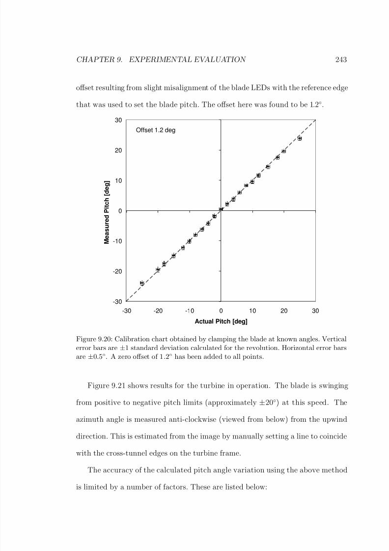
8/13/2019 Wholewhole
http://slidepdf.com/reader/full/wholewhole 268/396
CHAPTER 9. EXPERIMENTAL EVALUATION 243
offset resulting from slight misalignment of the blade LEDs with the reference edge
that was used to set the blade pitch. The offset here was found to be 1 .2.
-30
-20
-10
0
10
20
30
-30 -20 -10 0 10 20 30
Actual Pitch [deg]
M e a s u r e d P i t c h [ d
e g ]
Offset 1.2 deg
Figure 9.20: Calibration chart obtained by clamping the blade at known angles. Verticalerror bars are ±1 standard deviation calculated for the revolution. Horizontal error barsare ±0.5. A zero offset of 1.2 has been added to all points.
Figure 9.21 shows results for the turbine in operation. The blade is swinging
from positive to negative pitch limits (approximately ±20) at this speed. The
azimuth angle is measured anti-clockwise (viewed from below) from the upwind
direction. This is estimated from the image by manually setting a line to coincide
with the cross-tunnel edges on the turbine frame.
The accuracy of the calculated pitch angle variation using the above method
is limited by a number of factors. These are listed below:

8/13/2019 Wholewhole
http://slidepdf.com/reader/full/wholewhole 269/396

8/13/2019 Wholewhole
http://slidepdf.com/reader/full/wholewhole 270/396
CHAPTER 9. EXPERIMENTAL EVALUATION 245
• Lens distortion and location of the principal point in the image. Lens dis-
tortion may result in error, however the calculated pitch angle is relatively
insensitive to distortion as it is based on the separation between the LED
traces in the same part if the image, rather than the absolute position rela-
tive to the principal point. The two traces are likely to be locally offset by
a similar amount. For similar reasons, the pitch results are also quite insen-
sitive to the exact location of the principal point in the image. In this casethe principal point was assumed to be at the centre of the frame, however
deviations of up to 50 pixels resulted in maximum changes in calculated pitch
of less than 0.25. Greater accuracy may be obtained by use of a calibrated
camera, however even without this, results appear to be sufficiently accurate
for many uses.
• LED traces not coplanar. Any out-of-plane errors for either of the blade
LEDs or a reference LED will result in errors in the object space coordinates
calculated. These can be corrected for if the out-of-plane distance can be
measured by projecting image points back to the appropriate Z 2 plane. If one
of the LEDs is slightly out-of-plane, its trajectory is effectively shifted ‘ver-
tically’ in the image, and if no correction is made, an error in the calculated
pitch angle that varies approximately sinusoidally with azimuth results.
The magnitude of this error was estimated by generating trace images for
zero pitch, but with one LED 5 mm out-of-plane. Then traces were then
analysed with no out-of-plane correction. It was found that the calculated
pitch had a mean of −0.4 with amplitude 0.8. This is a reasonably small
error for quite a large out-of-plane distance for the present set up.

8/13/2019 Wholewhole
http://slidepdf.com/reader/full/wholewhole 271/396
CHAPTER 9. EXPERIMENTAL EVALUATION 246
• Fitting of ellipses to reference trace sample points. The minimisation of
algebraic distance ellipse fitting method is known to be biased, unlike a true
geometric distance minimisation method. However if care is taken to ensure
the sample points are positioned at accurately, the error involved here with
regularly spaced samples on a complete ellipse should be small.
• Estimation of the perspective transformation parameters from the reference
ellipses. The optimisation method used to find the ‘best’ values of viewingparameters to fit the reference ellipses are sensitive to the measured radii
of these trajectories and the quality of the ellipse fitting process. However
the accuracy of the calculated camera position can be checked by generating
predicted images of the reference circles and measuring the goodness of fit
to the image sample points.
• Overlap of blade LED traces. Small pitch angles where the leading and
trailing LEDs produce traces on the image that are close to each other and
sometimes overlapping would be better measured using LED’s of different
colour. This was tried initially but it was found that colours other than red
did not record as well in the digital image and produced difficulty for trace
detection.
• Smearing of traces. Another source of uncertainty is the ‘smearing’ of LED
traces over several revolutions being recorded in a single exposure. For exam-
ple a 2 second exposure at 180 rpm records 6 revolutions. Small fluctuations
in the LED paths visible to the naked eye were not recorded by the digital
camera, but must have caused the recorded traces to be wider and less dis-
tinct. To some extent however the uncertainty produced by this effect does

8/13/2019 Wholewhole
http://slidepdf.com/reader/full/wholewhole 272/396
CHAPTER 9. EXPERIMENTAL EVALUATION 247
directly reflect actual uncertainty in the pitch of the blade because the traces
are ‘average’ paths for the several revolutions recorded during the exposure.
• Refraction through wind tunnel window. All images were taken through the
Perspex window in the wind tunnel test section. Refraction of light through
the window may have contributed to distortion of the digital image.
By quantifying and minimising the above sources of error, the method has been
demonstrated to be sufficiently accurate to quantify the pitching response of the
turbine and gain insight into its performance characteristics.
9.5 Summary
A prototype turbine was designed and constructed for testing in the wind tunnel.
The turbine was designed to investigate the potential of the new design concepts
described in Chapter 3.
A design for the blades, which are subjected to large bending loads in operation,
was chosen through extensive theoretical analysis.
Instrumentation to measure the shaft torque and speed of the turbine was
incorporated. In addition, a new photogrammetric method of measuring the blade
pitch angle response pattern was conceived and developed.
Results of wind tunnel testing and comparison with theoretical results are
presented in Chapter 10.

8/13/2019 Wholewhole
http://slidepdf.com/reader/full/wholewhole 273/396
Chapter 10
Wind Tunnel Test Results
The prototype turbine described in Chapter 9 was tested in the wind tunnel at
UNSW with different designs of blade connecting components.
10.1 Rig Design Modifications
10.1.1 Pivot joint friction
Initially friction in the blade connections hampered starting performance of the
turbine. In order to reduce the friction, the bearing surfaces on which the weight
of the blades was taken were covered with plastic sheet to lower the coefficient of
friction. The plastic surfaces were then lubricated using first WD40 then a silicone
spray, however the moment required to initiate rotation (measured using a spring
balance) was still at least 0.8 Nm.
In order to reduce the friction further, the upper arms were modified so that
the weight of the blade was taken on a 6 mm brass screw head as the pivot
point for the blade. The upper turbine arms were given an initial upward angular
displacement using shims at the hub to offset the deflection under the weight of
the blade. This allowed the blade weight to be taken entirely at the upper arm,
with only the lightest contact remaining on the bearing surfaces at the lower arm.
This modification reduced the friction in the pivot joint by an order of magnitude.
Problems were encountered with this arrangement once greater turbine speeds
were attained. The increasing centrifugal load and the movement of the upper,
248

8/13/2019 Wholewhole
http://slidepdf.com/reader/full/wholewhole 274/396
CHAPTER 10. WIND TUNNEL TEST RESULTS 249
load-bearing, arms towards horizontal would cause the elastomeric component at
the lower end of the blade to ride up out of its housing. The blade would then jam
and pitching would cease.
In order to avoid this, a second load-bearing pivot point was installed at the
lower arm, so that the weight of the blade was shared. These modifications greatly
reduced the friction in the blade connection.
10.1.2 Brake friction
Even when the brake was released, the friction of the pads on the brake disc
produced an appreciable amount of residual torque, which had to be overcome
by the turbine. The minimum torque varied between 0.35 Nm and 1.5 Nm at
different azimuthal positions, producing a cyclic average of approximately 0.8 Nm.
The cyclical variation was due to misalignment of the brake disc on the shaft,
causing periodic binding between the brake pads. The cyclical average figure also
varied from run to run as braking caused movement of the calliper with respect to
the disc.
All of the early trials of the turbine suffered from excessive friction torque, ham-
pering attempts to achieve self-starting. The problem was addressed by grinding
the brake pads to chamfer the edges, first in the tangential direction and then
also in the radial direction. This reduced the area of the contact patch between
pad and disc and so reduced the tendency to bind when the disc was not in cor-
rect alignment. This reduced the cyclical average brake friction to approximately
0.15 Nm.
The brake calliper used was a rear motorcycle brake. While the residual friction
associated with it is of no consequence on a bike, the lack of springs to completely

8/13/2019 Wholewhole
http://slidepdf.com/reader/full/wholewhole 275/396
CHAPTER 10. WIND TUNNEL TEST RESULTS 250
release the brake was a significant problem for the turbine. Ultimately, the motor-
bike brake was replaced with one for a bicycle. This ensured that the brake pads
were not in contact with the disc when the brake was not applied.
10.1.3 Parasitic drag
Parasitic drag was found to be more significant than was anticipated. While the
radial arms themselves were produced with a streamlined profile, the fittings at
the outer ends produced considerable drag. It was intended to provide fairings for
this part of the rotor, however it was found that it was very difficult to reduce
the drag while still allowing unrestricted movement of the blade and access to the
connections.
Still air tests were conducted to estimate the magnitudes of aerodynamic drag
and brake friction. The deceleration of the turbine in still air at the end of a
wind tunnel run was used to calculate the torque arising from residual brake pad
friction and rolling element bearing friction. The values of aerodynamic drag and
dry friction coefficients of retarding torque were then estimated by numerically
differentiating the speed data, as described in Appendix C.
10.2 Experimental Procedure
The turbine was allowed to accelerate from rest without the brake applied until a
steady state speed was reached. In general, two different wind speeds were used:
approximately 5.7 m/s and 7.1 m/s, corresponding to dynamic pressures measured
at the pitot static tube of 2 mmH2O and 3 mmH2O respectively.
In general the turbine performance was assessed by allowing it to accelerate
under no-load conditions and calculating the torque from the acceleration as de-
scribed in Section 9.4.1.

8/13/2019 Wholewhole
http://slidepdf.com/reader/full/wholewhole 276/396
CHAPTER 10. WIND TUNNEL TEST RESULTS 251
The entire wind tunnel testing process was characterised by significant variation
in turbine performance under nominally identical conditions. The sensitivity of
performance to the blade pitch response meant that small changes in lubrication
or alignment of parts could have a significant effect on the measured output.
10.3 Results
10.3.1 Fixed blades
For reference the turbine was tested with the blades fixed in the zero-pitch position,
as a standard Darrieus turbine. The turbine did not operate at all, reaching a
runaway speed of only approximately 10 rpm at a wind speed of 7 m/s. Since no
external drive was included it was not possible to accelerate the turbine to a speed
at which the turbine may have been able to operate with fixed blades.
10.3.2 Type A component
TYPE A
Figure 10.1: Type A geometry
Initial testing was conducted with the Type A geometry elastomeric pieces (see
Figure 10.1). It was quickly apparent that the pieces were too stiff in torsion and
did not allow adequate pitching. Under no load, the turbine reached a steady state
speed of only 25 rpm at a wind speed of 7.1 m/s, a TSR of only 0.32.

8/13/2019 Wholewhole
http://slidepdf.com/reader/full/wholewhole 277/396
CHAPTER 10. WIND TUNNEL TEST RESULTS 252
In order to reduce the stiffness of the pieces, the stems of the elastomeric
components were modified to reduce their cross sectional area. However little
improvement was achieved. The maximum TSR at 7.0 m/s increased only to 0.41.
10.3.3 Type B component
TYPE B
R7 mm
C.G.
R20 mm
Figure 10.2: Type B geometry
The Type B geometry shown in Figure 10.2 was tested. Despite the much
smaller cross sectional area of the flexible stem compared to the Type A geometry,
the harder material made the component still too stiff in torsion. Insufficient pitch
amplitude for starting resulted. Again, the turbine failed to exceed TSR 0.4 under
no load.
It was therefore decided to test only the rolling profile portion of the Type B
geometry components by removing the flexible stems. The restoring moment was
then supplied only by inertial forces. This arrangement proved more successful.
The blade was able to pitch easily at start up, producing significant torque.
At a wind speed of 5.7 m/s, the turbine initially failed to accelerate beyond
approximately 20 rpm. At the higher wind speed, a similar steady-state velocity
was initially attained at approximately 30 rpm. These speeds correspond to tip
speed ratios of approximately 0.3 and 0.4 respectively.

8/13/2019 Wholewhole
http://slidepdf.com/reader/full/wholewhole 278/396
CHAPTER 10. WIND TUNNEL TEST RESULTS 253
0
0.01
0.02
0.03
0.04
0.05
0.06
0 0.2 0.4 0.6 0.8 1 1.2 1.4 1.6
TSR
C q
Type B
Hollow symbols 5.7 m/sSolid symbols 7.1 m/s
Figure 10.3: Measured torque coefficient versus tip speed ratio for the Type B purelyinertial geometry.
Efforts to reduce the friction and sticking in the blade connections and resid-
ual drag in the brake calliper allowed the turbine to accelerate to higher speeds.
However the turbine was still not able to accelerate beyond a tip speed ratio of ap-
proximately 1.5. Measured torque coefficient values for this geometry are presented
in Figure 10.3. The torque coefficient values were calculated using Equation 9.1.
Different symbols are used for separate test runs. Tests were conducted at two
different wind speeds: 5.7 m/s and 7.1 m/s.
Significant variation in the results is evident from run to run, especially in
the most successful run in which a maximum tip speed ratio of 1.5 was attained.
Despite this variation, all runs show a high starting torque with a trough around
TSR 0.4-0.5, a peak around TSR 0.6 and then a steady decline in torque towards
the maximum speed.

8/13/2019 Wholewhole
http://slidepdf.com/reader/full/wholewhole 279/396
CHAPTER 10. WIND TUNNEL TEST RESULTS 254
Initial testing with this arrangement produced vigorous pitching of the blades
at start up, but the blades were prone to becoming jammed at the extremes of
their range due to the force with which they hit the limits. This problem was
addressed using modified elastomeric components, where the flexible stem part
was used to cushion the stops (see Figure 10.4).
Figure 10.4: Use of the flexible stem to provide ‘cushioned’ pitch limits
This modification resulted in slightly improved starting performance, as well
as an increase in the runaway speed to approximately TSR 1.6 (see Figure 10.5).
It was thought that friction and resistance to blade pitching was still the main
problem preventing the turbine from reaching higher speeds, despite the fact that
minimal resistance was detectable when the turbine was stopped. The weight of
the blade was supported entirely at the upper arm and the lower arm was used
only to locate the blade horizontally. Increasing rotational speed resulted in a
reduction in the vertical deflection of the weight-bearing arm, causing an increase
in the distance between the arms and a tendency for the blade to jump out of its
housing. To avoid this a second pivot point was fitted to the lower arm so that the
weight of the blade could be shared. This arrangement had the desired effect and

8/13/2019 Wholewhole
http://slidepdf.com/reader/full/wholewhole 280/396
CHAPTER 10. WIND TUNNEL TEST RESULTS 255
-0.01
0
0.01
0.02
0.03
0.04
0.05
0.06
0 0.2 0.4 0.6 0.8 1 1.2 1.4 1.6 1.8
TSR
C q
Type B inertial/elastic
Figure 10.5: Measured torque coefficient versus tip speed ratio for the Type B withflexible stem
reduced misalignment and sticking of the blade at speed. Results of this improved
arrangement are shown in Figure 10.6.
The logged data for the most successful run and the corresponding power co-
efficient curve is shown in Figure 10.7. The maximum power coefficient achieved
was approximately 0.18 at a tip speed ratio of 2.9. There is a marked dip in output
between tip speed ratios 1.6 and 1.9. Once the turbine emerged from this trough it
accelerated rapidly up to a tip speed ratio of 3.2. At this point a load was applied
to control the speed of the turbine and to attempt to extract sustained power from
the shaft via the brake. However excessive load caused the turbine to decelerate
rapidly.
The trough in torque around TSR 1.6-1.7 was repeatedly observed in these
tests. True self-starting, with the turbine accelerating in a constant wind to a tip
speed ratio above 2.5, was achieved on three occasions. However in subsequent
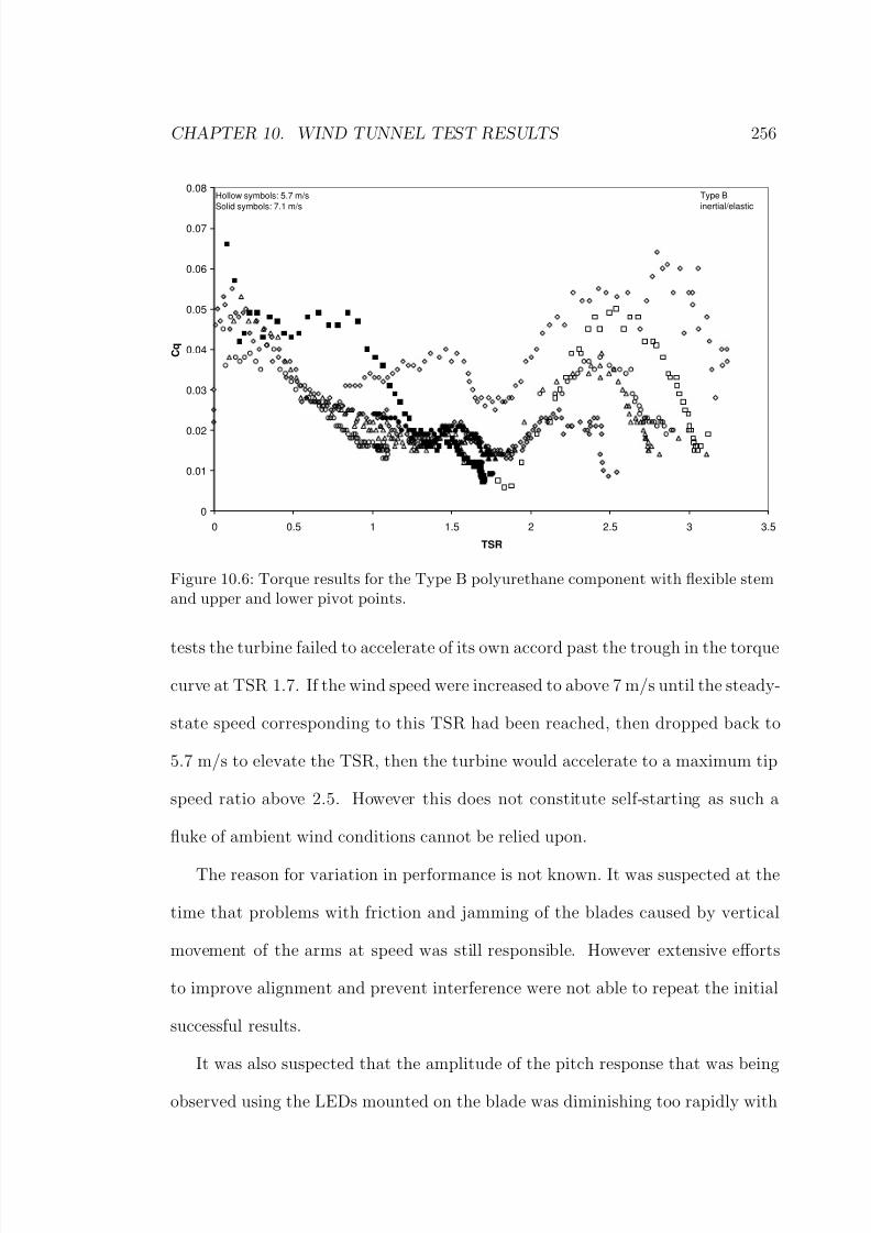
8/13/2019 Wholewhole
http://slidepdf.com/reader/full/wholewhole 281/396
CHAPTER 10. WIND TUNNEL TEST RESULTS 256
0
0.01
0.02
0.03
0.04
0.05
0.06
0.07
0.08
0 0.5 1 1.5 2 2.5 3 3.5
TSR
C q
Type B
inertial/elastic
Hollow symbols: 5.7 m/s
Solid symbols: 7.1 m/s
Figure 10.6: Torque results for the Type B polyurethane component with flexible stemand upper and lower pivot points.
tests the turbine failed to accelerate of its own accord past the trough in the torque
curve at TSR 1.7. If the wind speed were increased to above 7 m/s until the steady-
state speed corresponding to this TSR had been reached, then dropped back to
5.7 m/s to elevate the TSR, then the turbine would accelerate to a maximum tip
speed ratio above 2.5. However this does not constitute self-starting as such a
fluke of ambient wind conditions cannot be relied upon.
The reason for variation in performance is not known. It was suspected at the
time that problems with friction and jamming of the blades caused by vertical
movement of the arms at speed was still responsible. However extensive efforts
to improve alignment and prevent interference were not able to repeat the initial
successful results.
It was also suspected that the amplitude of the pitch response that was being
observed using the LEDs mounted on the blade was diminishing too rapidly with

8/13/2019 Wholewhole
http://slidepdf.com/reader/full/wholewhole 282/396
CHAPTER 10. WIND TUNNEL TEST RESULTS 257
0
20
40
60
80
100
120
140
160
180
200
0 100 200 300 400 500 600 700 800
Time [s]
T u r b i n e s p e e d [ r p m ]
0
5
10
15
20
25
W i n d s p e e d [ m / s ] a n d S h a f t t o r q u e [ N m ]
Speed
Torque
Wind
(a)
0
0.02
0.04
0.06
0.08
0.1
0.12
0.14
0.16
0.18
0.2
0 0.5 1 1.5 2 2.5 3 3.5
TSR
C p
(b)
Figure 10.7: Logged speed, torque and wind velocity data for a run of the Type Binertial/elastic geometry (a). The corresponding power coefficient curve (b).

8/13/2019 Wholewhole
http://slidepdf.com/reader/full/wholewhole 283/396
CHAPTER 10. WIND TUNNEL TEST RESULTS 258
increasing speed. Blade pitching was observed to effectively cease at the threshold
tip speed ratio of approximately 1.7 at which the turbine was stalling. This was
not predicted by the mathematical models. It was thought that the pitch response
may be reduced because of the compressibility of the polyurethane rolling profile,
resulting in rolling resistance.
Accordingly, new profile components were manufactured from High Density
Polyethylene (HDPE). The parts were NC milled to the same profile as the originalmoulded polyurethane components. These components were very much harder
than the polyurethane parts. The original ‘pillar’ components on which the profile
rolled, which were also moulded in polyurethane, were retained.
0
0.01
0.02
0.03
0.04
0.05
0.06
0.07
0 0.5 1 1.5 2 2.5 3 3.5
TSR
C q
Type B inertial HDPE
Figure 10.8: Torque results for the Type B High Density Polyethylene component.
Testing of the turbine with these components however did not yield radically
different results. The results are shown in Figure 10.8. The trough in the torque
curve between approximately TSR 1.5 and 1.7 was slightly negative, preventing

8/13/2019 Wholewhole
http://slidepdf.com/reader/full/wholewhole 284/396
CHAPTER 10. WIND TUNNEL TEST RESULTS 259
the turbine from accelerating up to running speed unassisted. However if the wind
speed were temporarily increased to accelerate the turbine, then dropped back to
‘leapfrog’ the negative torque zone, the turbine would then accelerate again to a
steady-state no-load TSR of 3.0.
The pitch response patterns for one of the turbine blades were measured using
the technique described in Section 9.4.3. The variation of pitch response with tip
speed ratio for one run is shown in Figure 10.9 for two different components. Theflexible stem results in less ‘dwell’ at high pitch angles at low tip speed ratios (a)
than is evident for the HDPE component (b). At higher tip speed ratios however
there is little difference between the two sets of responses.

8/13/2019 Wholewhole
http://slidepdf.com/reader/full/wholewhole 285/396
CHAPTER 10. WIND TUNNEL TEST RESULTS 260
0 90 180 270-90
0 3
TSR
AZIMUTH [deg]
PITCH
[deg]
30
20
10
0
-10
-20
-30
(a) Type B polyurethane geometry with flexible stem and upper and lower pivotpoints.
0 90 180 270-90
0 3
TSR
AZIMUTH [deg]
P
ITCH
[deg]
30
20
10
0
-10
-20
-30
(b) Type B HDPE components.
Figure 10.9: Measured blade pitch responses for two blade mounting geometries.

8/13/2019 Wholewhole
http://slidepdf.com/reader/full/wholewhole 286/396
CHAPTER 10. WIND TUNNEL TEST RESULTS 261
It was felt that the pitch response amplitude was decreasing too rapidly with
turbine speed and that performance would be improved by reducing the restoring
moment applied to the blades. Accordingly, the HDPE components were modified
to reduce the radius of curvature from 20 mm to 16 mm. This reduced the centre
of gravity radius Rcg from 7 mm to 3 mm, while maintaining the y0 offset at 13
mm (see Figure 10.10). The restoring moment should then be reduced to 3/7 of its
initial value. According to the predictions of the momentum theory mathematicalmodel, this level of torsional stiffness should be too low for the turbine to operate.
The frequency ratio calculated by Equation 7.1 should be greater than one and
the pitch response therefore out of phase with the variation in incidence at the
blade.
TYPE B II
C.G.
R3 mm
R16 mm
Figure 10.10: Type B II geometry
The performance of the turbine with the modified components (designated
Type B II) was however not greatly different from that with the original Type B
components. The torque coefficient data is shown in Figure 10.11(a), page 262.
The measured pitch response is shown in Figure 10.11(b).
In a further attempt to increase the pitch response amplitude, another set of
rolling profile components were manufactured from High Density Polyethylene.

8/13/2019 Wholewhole
http://slidepdf.com/reader/full/wholewhole 287/396
CHAPTER 10. WIND TUNNEL TEST RESULTS 262
-0.01
0.01
0.03
0.05
0.07
0.09
0 0.5 1 1.5 2 2.5 3 3.5
TSR
C q
Type B II
HDPE
(a) Torque coefficient.
0 90 180 270-90
0 3
TSR
AZIMUTH [deg]
PITCH
[deg]
30
20
10
0
-10
-20
-30
(b) Measured pitch response.
Figure 10.11: Torque and pitch results for the Type B II modified geometry.

8/13/2019 Wholewhole
http://slidepdf.com/reader/full/wholewhole 288/396
CHAPTER 10. WIND TUNNEL TEST RESULTS 263
In this geometry, labelled Type B III and shown in Figure 10.12, the radius of
curvature over a range if ±12 either side of the ‘nose’ was 14 mm, while outside
this range the radius was 16 mm. This geometry produced a centre of gravity
offset of just 1 mm at the nose. It was desired to test whether the concept of
tailoring the profile could result in different pitch response behaviour at different
tip speed ratios.
TYPE B III
C.G.
R14 mm
24o
R16 mm
R1 mm
R16 mm
Figure 10.12: Type B III geometry
The torque coefficient results for this geometry are shown in Figure 10.13(a)
and the measured pitch response is shown in Figure 10.14(a). The pitch response
exhibits characteristics of a reduced restoring moment: the amplitude is greater
at a given tip speed ratio than for the Type B and Type B II geometries; also the
phase lag of the response is greater, indicating the blade is operating closer to its
natural frequency. The turbine however did not progress beyond tip speed ratio
1.7.
Springs were then fitted to the blades to supplement the inertial restoring
moment, to see how this would affect performance. The aim was to increase the
torsional stiffness at low tip speed ratios, while allowing greater pitching at higher
speeds. As the added springs acted independently of centrifugal force, they are

8/13/2019 Wholewhole
http://slidepdf.com/reader/full/wholewhole 289/396
CHAPTER 10. WIND TUNNEL TEST RESULTS 264
-0.02
-0.01
0
0.01
0.02
0.03
0.04
0.05
0.06
0.07
0.08
0.09
0.1
0 0.5 1 1.5 2 2.5 3TSR
C q
Type B III
HDPE
(a) Torque coefficient results
0 90 180 270-90
0 3
TSR
AZIMUTH [deg]
PITCH
[deg]
30
20
10
0
-10
-20
-30
(b) Measured pitch response
Figure 10.13: Results for the Type B III geometry.

8/13/2019 Wholewhole
http://slidepdf.com/reader/full/wholewhole 290/396
CHAPTER 10. WIND TUNNEL TEST RESULTS 265
-0.02
-0.01
0
0.01
0.02
0.03
0.04
0.05
0.06
0.07
0.08
0.09
0.1
0 0.5 1 1.5 2 2.5 3
TSR
C q
Type B III
HDPE
inertial/elastic
(a) Torque coefficient results
0 90 180 270-90
0 3
TSR
AZIMUTH [deg]
PITCH
[deg]
30
20
10
0
-10
-20
-30
(b) Measured pitch response
Figure 10.14: Results the Type B III modified geometry with additional spring.

8/13/2019 Wholewhole
http://slidepdf.com/reader/full/wholewhole 291/396
CHAPTER 10. WIND TUNNEL TEST RESULTS 266
able to add a constant amount of stiffness that is significant at low speeds but
becomes insignificant as the inertial component restoring moment increases.
The results are shown in Figures 10.13(b) and 10.14(b). This addition allowed
the turbine to properly self-start on its initial test run, however subsequent runs
failed to accelerate beyond the torque trough at TSR 1.8 without increasing then
dropping the wind speed to jump the negative zone. Once above TSR 2, the
turbine accelerated to a runaway speed of approximately TSR 2.7.

8/13/2019 Wholewhole
http://slidepdf.com/reader/full/wholewhole 292/396
CHAPTER 10. WIND TUNNEL TEST RESULTS 267
10.3.4 Type C geometry
R7 mmC.G.
Figure 10.15: Type C geometry
Testing of the turbine with the Type C geometry was expected to yield similar
performance to that obtained with the Type B geometry. The Type C component
also had a circular arc rolling profile, with the centre of mass at a radius of 7 mm,
as shown in Figure 10.15. The y0 value was in this case zero.
As for the Type B geometry, the components in their original form were too
stiff due to the elastic portion of the parts. Accordingly, as before, flexible stems
of the components were cut and allowed to act as cushions on the pitch limits of
the blade. In this case, the flexible stem made contact with the side of the housing
at a pitch angle of approximately 14, with a pitch limit of 28.
Testing produced good low speed performance, but the turbine failed to accel-
erate beyond a tip speed ratio of 1.8. Significantly higher torque was produced
in this speed range than for the Type B geometry. Torque coefficient results are
plotted in Figure 10.16(a). For this geometry the results were relatively consistent,
with maximum torque occurring at start-up, a dip in torque at TSR 0.5
The measured pitch responses for this geometry are shown in Figure 10.16(b).

8/13/2019 Wholewhole
http://slidepdf.com/reader/full/wholewhole 293/396
CHAPTER 10. WIND TUNNEL TEST RESULTS 268
0
0.01
0.02
0.03
0.04
0.05
0.06
0.07
0.08
0.09
0.1
0 0.2 0.4 0.6 0.8 1 1.2 1.4 1.6 1.8 2
TSR
C q
Type C
inertial/elastic
Hollow symbols: 5.7 m/s
Solid symbols: 7.1 m/s
(a) Torque coefficient results
0 90 180 270-90
0 3
TSR
AZIMUTH [deg]
PITCH
[deg]
30
20
10
0
-10
-20
-30
(b) Measured pitch response
Figure 10.16: Torque coefficient data and measured pitch response for the Type C ge-
ometry. Different symbols are used for separate test runs.

8/13/2019 Wholewhole
http://slidepdf.com/reader/full/wholewhole 294/396
CHAPTER 10. WIND TUNNEL TEST RESULTS 269
10.4 Comparison with Theoretical Results
The performance of the prototype turbine was predicted using both the Double
Multiple Streamtube (DMS) model and the vortex model.
The Double Multiple Streamtube model by its nature predicts steady-state
performance. It is therefore not strictly applicable to the prediction of performance
of the turbine while accelerating. Neither the blade pitch response nor the unsteady
wake can be assumed to be the same as those under steady conditions at a given
tip speed ratio. Nevertheless, where acceleration is small the difference may be
minimal and so the results are presented here for comparison. The vortex model
on the other hand is designed to deal with unsteady behaviour.
The parameters used for the theoretical predictions are shown in Table 10.1.
Parameter Value
Radius 0.87 mHeight 1.3 mBlades 3Chord 150 mmBlade mass 7.36 kgBlade moment of inertia 0.035 kgm2
Rac 20.5 mmDamping coefficient 0.015 Nm
rad/s
Friction coefficient 0.0002
Table 10.1: Prototype turbine parameters
The friction coefficient is defined as the ratio of the frictional moment on the
blade to the radial reaction at the blade connection.
The predicted performance of the turbine at a wind speed of 7 m/s with the
Type B and Type C geometry rolling profile components under ideal conditions
is shown in Figure 10.17. Here parasitic drag and blade friction have been set to
zero.

8/13/2019 Wholewhole
http://slidepdf.com/reader/full/wholewhole 295/396
CHAPTER 10. WIND TUNNEL TEST RESULTS 270
0
0.02
0.04
0.06
0.08
0.1
0.12
0 0.5 1 1.5 2 2.5 3 3.5 4
TSR
C q
Type B
Type C
7 m/s
(a) Torque coefficient
0
0.05
0.1
0.15
0.2
0.25
0.3
0 0.5 1 1.5 2 2.5 3 3.5 4
TSR
C p
Type B
Type C
7 m/s
(b) Power coefficient
Figure 10.17: Torque and power coefficient predicted by the Double Multiple Stream-tube (DMS) mathematical model under ideal conditions (ie no parasitic drag, no bladefriction)

8/13/2019 Wholewhole
http://slidepdf.com/reader/full/wholewhole 296/396
CHAPTER 10. WIND TUNNEL TEST RESULTS 271
10.4.1 Type B component
-0.06
-0.04
-0.02
0
0.02
0.04
0.06
0.08
0.1
0 0.5 1 1.5 2 2.5 3
TSR
C q
Experiment 7.1 m/s
Experiment 5.7 m/s
DMS
Vortex
Type B inertial HDPE
Figure 10.18: Torque coefficient predicted by the Double Multiple Streamtube (DMS)
and vortex mathematical models, compared with experimental data
The DMS results are shown in Figure 10.18. The predicted values are net
torque, parasitic drag and bearing friction, as estimated from turbine run-down
tests (see Appendix C), have been subtracted.
Agreement between experimental and theoretical results from both models is
reasonable for tip speed ratios less than 1.7. Both predict a high starting torque,
dropping to a local minimum at approximately TSR 0.5. Both models predict
a recovery of torque, with a local maximum at TSR 1.0, then a decline to zero
torque at approximately TSR 1.7. These predictions match the general trends of
the experimental data. The DMS model slightly overpredicts the torque, while the
vortex model predicts a dip in torque between TSR 1.1 and 1.2 that is not evident
in the measured data.

8/13/2019 Wholewhole
http://slidepdf.com/reader/full/wholewhole 297/396
CHAPTER 10. WIND TUNNEL TEST RESULTS 272
The main discrepancy between theoretical and experimental results is for tip
speed ratios greater than 1.7. Both mathematical models predict a steady pro-
gression to increasingly large negative values. By contrast, the turbine exhibited a
tendency to dip to zero torque at approximately TSR 1.7, but was able to produce
positive torque for TSRs between 2 and 3.
To gain insight into the cause of this discrepancy, the pitch response for one of
the experimental runs was compared with theoretical predictions. These resultsare presented in Figures 10.19, 10.20 and 10.21.
The predicted pitch responses for the DMS and vortex models are very similar
for each tip speed ratio, despite the fact that the DMS model predicts the steady-
state pattern while the vortex model predicts what is a transient pattern for the
single revolution closest to the tip speed ratio of the measured pattern.
These predictions are made with the values of the damping coefficient and
friction coefficient adjusted to best match the measured values. In the absence
of damping and friction in the blade connection, the predicted pitch response is
greater in amplitude than the measured response at almost all speeds. Only with
the addition of friction does the blade settle to virtually zero amplitude at TSR
3.0, as was measured. It is clear that if the damping and friction are adjusted to
match the measured pitch amplitude, the phase of the response changes. For all tip
speed ratios shown in Figures 10.19, 10.20 and 10.21 the predicted pitch response
lags the measured pitch response by approximately 30 to 40. The shape of the
predicted pitch response is otherwise fairly similar to the measured response. The
predicted amplitude is slightly greater than the measured amplitude at most tip
speed ratios. The asymmetry in the pitch response is slightly underpredicted. At

8/13/2019 Wholewhole
http://slidepdf.com/reader/full/wholewhole 298/396
CHAPTER 10. WIND TUNNEL TEST RESULTS 273
-30
-20
-10
0
10
20
30
-90 0 90 180 270
Azimuth [deg]
P i t c h
[ d e g ]
Experiment TSR 0.3
DMS
Vortex
TSR 0.3
-30
-20
-10
0
10
20
30
-90 0 90 180 270
Azimuth [deg]
P i t c h
[ d e g ]
Experiment TSR 0.57
DMS
Vortex
TSR 0.6
-30
-20
-10
0
10
20
30
-90 0 90 180 270
Azimuth [deg]
P i t c h
[ d e g ]
Experiment TSR 0.73
DMS
Vortex
TSR 0.7
Figure 10.19: Measured and predicted pitch responses, Type B, TSR 0.3 - 0.7

8/13/2019 Wholewhole
http://slidepdf.com/reader/full/wholewhole 299/396
CHAPTER 10. WIND TUNNEL TEST RESULTS 274
-30
-20
-10
0
10
20
30
-90 0 90 180 270
Azimuth [deg]
P i t c h
[ d e g ]
Experiment TSR 1.1DMS
Vortex
TSR 1.1
-30
-20
-10
0
10
20
30
-90 0 90 180 270
Azimuth [deg]
P i t c h
[ d e g ]
Experiment TSR 1.3
DMS
Vortex
TSR 1.3
-30
-20
-10
0
10
20
30
-90 0 90 180 270
Azimuth [deg]
P i t c h
[ d e g ]
Experiment TSR 1.6
DMS
Vortex
TSR 1.6
Figure 10.20: Measured and predicted pitch responses, Type B, TSR 1.1 - 1.6

8/13/2019 Wholewhole
http://slidepdf.com/reader/full/wholewhole 300/396
CHAPTER 10. WIND TUNNEL TEST RESULTS 275
-30
-20
-10
0
10
20
30
-90 0 90 180 270Azimuth [deg]
P i t c h
[ d e g ]
Experiment TSR 2.12
DMS
Vortex
TSR 2.1
-30
-20
-10
0
10
20
30
-90 0 90 180 270
Azimuth [deg]
P i t c h
[ d e g ]
Experiment TSR 2.5
DMS
Vortex
TSR 2.5
-30
-20
-10
0
10
20
30
-90 0 90 180 270
Azimuth [deg]
P i t c h
[ d e g ]
Experiment TSR 3
DMS
Vortex
TSR 3
Figure 10.21: Measured and predicted pitch responses, Type B, TSR 2.1 - 3.0

8/13/2019 Wholewhole
http://slidepdf.com/reader/full/wholewhole 301/396
CHAPTER 10. WIND TUNNEL TEST RESULTS 276
TSR 3, the blade was observed to settle to an almost constant pitch of approx-
imately -3, while the momentum and vortex models predict an almost constant
pitch of approximately -1.
10.4.2 Type B II geometry
The theoretical results for the Type B II geometry predict that the restoring
moment produced by this geometry should be too small. The frequency ratio for
the blades should be greater than one, resulting in pitch response out of phase
with the natural angle of incidence variation and negative torque for tip speed
ratios greater than approximately 0.4. Below this speed the pitch stops limit
the phase lag and result in positive torque at start up. Figure 10.22 shows the
comparison between theoretical and experimental results for torque coefficient for
this geometry. It is evident that agreement is good for tip speed ratios up to 0.4.
At this speed the torque is almost zero. While in the wind tunnel the torque
recovered at higher speeds and a maximum tip speed ratio of three was reached,
both the mathematical models predict increasingly large negative torque.
The pitch responses shown in Figures 10.23 to 10.25 (pages 278 to 280) show the
large phase difference, at times more than 90, between the measured and predicted
patterns, especially above TSR 0.4. It is the large phase lag of predicted pitch
response that produces the negative predicted torque. The measured response
however exhibits a much smaller lag angle. This phase difference suggests a greater
than predicted restoring moment acting in the experimental rig. To test this
hypothesis, the simulations were repeated with an additional restoring moment
added to the inertial moment supplied by the rolling profile. The best agreement
with the measured pitch responses was found by setting the additional moment
proportional to centrifugal force at 0.006 (Nm/rad)/N. The new responses are

8/13/2019 Wholewhole
http://slidepdf.com/reader/full/wholewhole 302/396
CHAPTER 10. WIND TUNNEL TEST RESULTS 277
-0.1
-0.08
-0.06
-0.04
-0.02
0
0.02
0.04
0.06
0.08
0.1
0.12
0.14
0 0.5 1 1.5 2 2.5 3
TSR
C q
Experiment
DMS
Vortex
Type B II
HDPE
Figure 10.22: Measured and predicted torque coefficient, Type B II geometry
shown in Figures 10.26 and 10.27 (pages 281 to 282). The reduced phase angle is
evident.
The predicted torque coefficient with this additional spring moment is shown
in Figure 10.28 (page 283). The agreement with experimental data is improved,
though the torque above TSR 1.7 is still negative.

8/13/2019 Wholewhole
http://slidepdf.com/reader/full/wholewhole 303/396
CHAPTER 10. WIND TUNNEL TEST RESULTS 278
-30
-20
-10
0
10
20
30
-90 0 90 180 270
Azimuth [deg]
P i t c h
[ d e g ]
Experiment
DMS
Vortex
TSR 0.3
-30
-20
-10
0
10
20
30
-90 0 90 180 270
Azimuth [deg]
P i t c h
[ d e g ]
Experiment
DMS
Vortex
TSR 0.4
-30
-20
-10
0
10
20
30
-90 0 90 180 270
Azimuth [deg]
P i t c h
[ d e g ]
Experiment
DMS
Vortex
TSR 0.7
Figure 10.23: Measured and predicted pitch responses, Type B II, TSR 0.3 - 0.7

8/13/2019 Wholewhole
http://slidepdf.com/reader/full/wholewhole 304/396
CHAPTER 10. WIND TUNNEL TEST RESULTS 279
-30
-20
-10
0
10
20
30
-90 0 90 180 270
Azimuth [deg]
P i t c h
[ d e g ]
Experiment
DMS
Vortex
TSR 0.9
-30
-20
-10
0
10
20
30
-90 0 90 180 270
Azimuth [deg]
P i t c h
[ d e g ]
Experiment
DMS
Vortex
TSR 1.4
-30
-20
-10
0
10
20
30
-90 0 90 180 270
Azimuth [deg]
P i t c h
[ d e g ]
Experiment
DMS
Vortex
TSR 1.6
Figure 10.24: Measured and predicted pitch responses, Type B II, TSR 0.9 - 1.6

8/13/2019 Wholewhole
http://slidepdf.com/reader/full/wholewhole 305/396
CHAPTER 10. WIND TUNNEL TEST RESULTS 280
-30
-20
-10
0
10
20
30
-90 0 90 180 270
Azimuth [deg]
P i t c h
[ d e g ]
Experiment
DMS
Vortex
TSR 2.0
-30
-20
-10
0
10
20
30
-90 0 90 180 270
Azimuth [deg]
P i t c h
[ d e g ]
Experiment
DMS
Vortex
TSR 2.3
-30
-20
-10
0
10
20
30
-90 0 90 180 270
Azimuth [deg]
P i t c h
[ d e g ]
Experiment
DMS
Vortex
TSR 2.7
Figure 10.25: Measured and predicted pitch responses, Type B II, TSR 2.0 - 2.7

8/13/2019 Wholewhole
http://slidepdf.com/reader/full/wholewhole 306/396
CHAPTER 10. WIND TUNNEL TEST RESULTS 281
-30
-20
-10
0
10
20
30
-90 0 90 180 270
Azimuth [deg]
P i t c h
[ d e g ]
Experiment
DMS
Vortex
TSR 0.3
-30
-20
-10
0
10
20
30
-90 0 90 180 270
Azimuth [deg]
P i t c h
[ d e g ]
Experiment
DMS
Vortex
TSR 0.4
-30
-20
-10
0
10
20
30
-90 0 90 180 270
Azimuth [deg]
P i t c h
[ d e g ]
Experiment
DMS
Vortex
TSR 0.7
Figure 10.26: Measured pitch responses for the Type B II geometry compared withpredicted pitch responses for Type B II with additional spring; TSR 0.3 - 0.7

8/13/2019 Wholewhole
http://slidepdf.com/reader/full/wholewhole 307/396
CHAPTER 10. WIND TUNNEL TEST RESULTS 282
-30
-20
-10
0
10
20
30
-90 0 90 180 270
Azimuth [deg]
P i t c h
[ d e g ]
Experiment
DMSVortex
TSR 0.9
-30
-20
-10
0
10
20
30
-90 0 90 180 270
Azimuth [deg]
P i t c h
[ d e g ]
Experiment
DMS
Vortex
TSR 1.4
-30
-20
-10
0
10
20
30
-90 0 90 180 270
Azimuth [deg]
P i t c h
[ d e g ]
Experiment
DMS
Vortex
TSR 1.6
Figure 10.27: Measured pitch responses for the Type B II geometry compared withpredicted pitch responses for Type B II with additional spring; TSR 0.9 - 1.6.

8/13/2019 Wholewhole
http://slidepdf.com/reader/full/wholewhole 308/396
CHAPTER 10. WIND TUNNEL TEST RESULTS 283
-0.1
-0.08
-0.06
-0.04
-0.02
0
0.02
0.04
0.06
0.08
0.1
0.12
0.14
0 0.5 1 1.5 2 2.5 3
TSR
C q
Experiment
Vortex
DMS
Figure 10.28: Measured torque coefficient for the Type B II geometry compared withpredicted torque for Type B II with additional spring
If the same additional spring restoring moment is applied to the simulations
for the original Type B geometry, the agreement between measured and predicted
pitch response patterns similarly improves, as shown in Figures 10.29, 10.30 and
10.31 (pages 284 to 286). The predicted torque, shown in Figure 10.32 (page 287),
however now over-estimates the actual torque, up to TSR 2 where the torque
becomes negative.

8/13/2019 Wholewhole
http://slidepdf.com/reader/full/wholewhole 309/396
CHAPTER 10. WIND TUNNEL TEST RESULTS 284
-30
-20
-10
0
10
20
30
-90 0 90 180 270
Azimuth [deg]
P i t c h
[ d e g ]
Experiment TSR 0.3
DMS
Vortex
TSR 0.3
-30
-20
-10
0
10
20
30
-90 0 90 180 270
Azimuth [deg]
P i t c h
[ d e g ]
Experiment TSR 0.57
DMS
Vortex
TSR 0.6
-30
-20
-10
0
10
20
30
-90 0 90 180 270
Azimuth [deg]
P i t c h
[ d e g ]
Experiment TSR 0.73
DMS
Vortex
TSR 0.7
Figure 10.29: Measured pitch responses for the Type B geometry compared with pre-dicted pitch responses for Type B with additional spring; TSR 0.3 - 0.7

8/13/2019 Wholewhole
http://slidepdf.com/reader/full/wholewhole 310/396
CHAPTER 10. WIND TUNNEL TEST RESULTS 285
-30
-20
-10
0
10
20
30
-90 0 90 180 270
Azimuth [deg]
P i t c h
[ d e g ]
Experiment TSR 1.1
DMS
Vortex
TSR 1.1
-30
-20
-10
0
10
20
30
-90 0 90 180 270
Azimuth [deg]
P i t c h
[ d e g ]
Experiment TSR 1.3
DMS
Vortex
TSR 1.3
-30
-20
-10
0
10
20
30
-90 0 90 180 270
Azimuth [deg]
P i t c h
[ d e g ]
Experiment TSR 1.6
DMS
Vortex
TSR 1.6
Figure 10.30: Measured pitch responses for the Type B geometry compared with pre-
dicted pitch responses for Type B with additional spring; TSR 1.1 - 1.6.
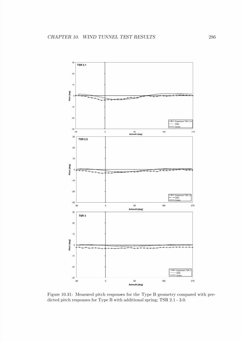
8/13/2019 Wholewhole
http://slidepdf.com/reader/full/wholewhole 311/396
CHAPTER 10. WIND TUNNEL TEST RESULTS 286
-30
-20
-10
0
10
20
30
-90 0 90 180 270
Azimuth [deg]
P i t c h
[ d e g ]
Experiment TSR 2.12
DMS
Vortex
TSR 2.1
-30
-20
-10
0
10
20
30
-90 0 90 180 270
Azimuth [deg]
P i t c h
[ d e g ]
Experiment TSR 2.5
DMS
Vortex
TSR 2.5
-30
-20
-10
0
10
20
30
-90 0 90 180 270
Azimuth [deg]
P i t c h
[ d e g ]
Experiment TSR 3
DMS
Vortex
TSR 3
Figure 10.31: Measured pitch responses for the Type B geometry compared with pre-
dicted pitch responses for Type B with additional spring; TSR 2.1 - 3.0.

8/13/2019 Wholewhole
http://slidepdf.com/reader/full/wholewhole 312/396
CHAPTER 10. WIND TUNNEL TEST RESULTS 287
-0.06
-0.04
-0.02
0
0.02
0.04
0.06
0.08
0.1
0 0.5 1 1.5 2 2.5 3
TSR
C q
Experiment 7.1 m/s
Experiment 5.7 m/sVortex 5.7 m/s
DMS 5.7 m/s
Figure 10.32: Measured torque coefficient for the Type B geometry compared withpredicted torque for Type B with additional spring
10.4.3 Type C component
Comparison between predicted and measured torque coefficients for the Type C
geometry is shown in Figure 10.33. Both the DMS and vortex model predictions
follow the general trend of the experimental data and predict the maximum tip
speed ratio fairly well.
The predicted and measured pitch response patterns for a range of tip speedratios is shown in Figures 10.34 and 10.35 (pages 289 and 290). Unlike the results
for the Type B and Type B II geometries, there is no significant phase differ-
ence between the predicted and measured pitch responses. This suggests there
is no significant additional restoring moment acting that is not included in the
mathematical models.
The vortex model predicted torque exhibits oscillations in the range TSR 0.7
- TSR 1.1. The exact location and magnitude of the peaks and troughs in the

8/13/2019 Wholewhole
http://slidepdf.com/reader/full/wholewhole 313/396
CHAPTER 10. WIND TUNNEL TEST RESULTS 288
0
0.02
0.04
0.06
0.08
0.1
0.12
0.14
0 0.2 0.4 0.6 0.8 1 1.2 1.4 1.6 1.8 2
TSR
C q
Experiment 5.7 m/s
Experiment 7.1 m/s
DMS 5.7 m/s
Vortex 5.7 m/s
Type C inertial/elastic
Figure 10.33: Measured and predicted torque coefficient, Type C geometry
torque curve in this region are dependent on the initial conditions set for the run.
To illustrate this, two runs were conducted with an initial velocity corresponding
to a tip speed ratio of 0.01. In one run, the blades were given an initial pitch of
zero degrees and for the other they were all set to +14. The predicted speed-time
histories and corresponding torque coefficient curves are shown in Figure 10.36. It
is evident that the initial conditions affect the output of the turbine throughout
the run, even producing different final speeds after 250 seconds of simulated time.
While the general nature of the torque coefficient curves are the same, the exact
locations of the various peaks, corresponding to ‘spurts’ in the speed histories, are
different. This indicates that for the accelerating turbine the pitch response at a
given speed is transient and may result in appreciably different torques from those
produced under different unsteady conditions or at steady-state at that speed.

8/13/2019 Wholewhole
http://slidepdf.com/reader/full/wholewhole 314/396
CHAPTER 10. WIND TUNNEL TEST RESULTS 289
-30
-20
-10
0
10
20
30
-90 0 90 180 270
Azimuth [deg]
P i t c h
[ d e g ]
ExperimentDMS
Vortex
TSR 0.4
-30
-20
-10
0
10
20
30
-90 0 90 180 270
Azimuth [deg]
P i t c h
[ d e g ]
Experiment
DMS
Vortex
TSR 0.7
-30
-20
-10
0
10
20
30
-90 0 90 180 270
Azimuth [deg]
P i t c h
[ d e g ]
Experiment
DMS
Vortex
TSR 1.0
Figure 10.34: Measured and predicted pitch responses, Type C, TSR 0.4 - 1.0

8/13/2019 Wholewhole
http://slidepdf.com/reader/full/wholewhole 315/396

8/13/2019 Wholewhole
http://slidepdf.com/reader/full/wholewhole 316/396
CHAPTER 10. WIND TUNNEL TEST RESULTS 291
0
2
4
6
8
10
12
0 50 100 150 200 250
Time [s]
S p e e d [
r a d / s ]
Initial pitch 0 degrees
Initial pitch +14 degrees
(a)
0
0.02
0.04
0.06
0.08
0.1
0.12
0.14
0.16
0 0.2 0.4 0.6 0.8 1 1.2 1.4 1.6 1.8
TSR
C q
Initial pitch 0 degrees
Initial pitch +14 degrees
(b)
Figure 10.36: Comparison of the speed-time histories (a) and corresponding torquecoefficient-TSR curves (b) for the Type C geometry component with two different initialconditions.

8/13/2019 Wholewhole
http://slidepdf.com/reader/full/wholewhole 317/396
CHAPTER 10. WIND TUNNEL TEST RESULTS 292
its bearing surface. Since this contact had to transmit only the weight of the
blade due to gravity rather than its centrifugal weight, and because vibration was
expected to reduce resistance under operating conditions, friction at this point was
not expected to be high.
The pitch response patterns measured during operation however indicate ap-
preciable friction that is proportional to centrifugal load. This must be due to
rolling resistance caused by deformation of the rolling profile component and thesurface on which it rolls. This deformation produces a finite area contact patch and
moves the location of the resultant normal contact force forward (in the direction
of motion). There is then effectively an additional moment retarding the rolling
motion. The magnitude of this resistance is dependent on the geometry and mate-
rial properties of the two components. The initial rolling profile components were
manufactured in polyurethane in order to incorporate an elastic restoring moment
through the flexibility of the material. However this flexibility would have resulted
in increased contact patch deformation and increased rolling resistance. This point
was realised during testing and replacement parts manufactured in much harder
High Density Polyethylene. The polyurethane mating components however were
retained and little change was measured in the pitching behaviour.
In order to reduce such resistance both the rolling profile component and the
mating part should be manufactured in a harder material, possibly steel. The
wearing properties of the two materials must be considered. Wear resistance was
a factor in the selection of polyurethane as the original material.
Some aspects of the turbine performance cannot be attributed to friction. The
fact that the Type B II and Type B III geometry components produced success-

8/13/2019 Wholewhole
http://slidepdf.com/reader/full/wholewhole 318/396

8/13/2019 Wholewhole
http://slidepdf.com/reader/full/wholewhole 319/396
CHAPTER 10. WIND TUNNEL TEST RESULTS 294
of incidence angle variation. The incident wind swings around the trailing edge
of the blade as it travels downwind much more rapidly than it travels around the
leading edge as it travels upwind. To take a sailing analogy, the angle of attack
changes much faster as the blade ‘gybes’ than it does as it ‘tacks’. This results
in a more gradual motion of the blade from its positive limit to the negative limit
than in the reverse direction.
As tip speed ratio increases, the deceleration of the flow through the turbinebecomes more pronounced. For a high solidity turbine like that tested here, most
of the deceleration occurs at the upwind half of the blades’ orbit. By the time the
flow reaches the blades in the downwind half, most of its energy has already been
extracted. This results in smaller angles of attack on the downwind pass than
on the upwind pass. The positive pitch excursion that occurs in the downwind
pass can then be expected to be smaller than the negative angle excursion on
the upwind pass. This effect should become more pronounced as tip speed ratio
increases.
This effect however cannot explain a constant negative pitch offset being main-
tained with virtually zero pitch amplitude. The decelerated flow experienced by
the blades in the downwind pass only reduces the disturbing aerodynamic moment.
If the inertial restoring moment is moving the blade towards zero pitch, then the
pitch should approach zero, not adopt a constant negative value.
The only factor that would produce a constant negative pitch offset is the
aerodynamic force on the blade that is pivoted about a point forward of its aero-
dynamic centre. The zero pitch line is defined as being perpendicular to the radius
through the pivot axis. Here the quarter chord point of the blade is 20.5 mm aft
of the pivot axis. At zero pitch there is therefore a some negative angle of attack

8/13/2019 Wholewhole
http://slidepdf.com/reader/full/wholewhole 320/396
CHAPTER 10. WIND TUNNEL TEST RESULTS 295
experienced at the aerodynamic centre. This would cause the blade to adopt some
small negative pitch angle to find the orientation of least resistance as the turbine
spins, even in still air. In addition, the curvature of the flow experienced by a
blade moving in a circular path causes further negative deflection of the blade.
The observed decrease in the pitch offset with decreasing turbine speed as the
turbine decelerates from speed in still air is in keeping with the idea that these
effects contribute to the offset.Both of these effects are handled in the mathematical models. The calculated
angle of attack takes into account the distance between the pivot axis and the
aerodynamic centre and the flow curvature method of Migliore (1984) modifies
the effective angle of attack. The inclusion of friction in the model successfully
reproduces the settling to an almost constant negative pitch angle at high tip speed
ratios, albeit of a smaller magnitude than was measured.
Blockage
The other major area of discrepancy between predicted and experimental perfor-
mance was for tip speed ratios greater than 1.7. While the mathematical models
predict negative torque at these speeds, positive torque was produced experimen-
tally. The mathematical models predict positive ‘gross’ torque, but when parasitic
drag is subtracted, the net torque is negative.
The reason for this discrepancy is not known. The quality of agreement at lower
tip speed ratios is reasonable. It is possible that the effects of blockage in the wind
tunnel contribute to this difference. The constraints of the tunnel walls may force
the flow velocity to be higher than would be the case in the open, especially in the
downwind half of the turbine.

8/13/2019 Wholewhole
http://slidepdf.com/reader/full/wholewhole 321/396
CHAPTER 10. WIND TUNNEL TEST RESULTS 296
Grylls et al. (1978) however attributed a lower than predicted maximum torque
to blockage effects. They tested a ‘cycloturbine’, with a cam driving a preset sched-
ule of pitch variation, in a wind tunnel and measured the power coefficient using a
dynamometer. They measured a maximum power coefficient of approximately 0.2.
This was lower than their predicted value of more than 0.3. They speculated that
the discrepancy may be due to the wind tunnel walls preventing the full expansion
of the wake that would occur under free conditions. Their turbine had a diameterof 2.4 m and a height of 1.6 m. The wind tunnel test section measured 10 ft x 12
ft (3.05 m x 3.66 m), giving a blockage of approximately 34%. Grylls et al. state
that:
“It is believed that the wake of the rotor is unable to expand any
further than the size corresponding to a 20% power extraction. . .
Our experience . . . suggests that blockage does not give an increased
speed at the rotor, but rather higher speed in the wake than antici-
pated.”
The maximum Cp recorded by Kirke (1998) for the 2 m diameter turbine
he tested in the wind tunnel was approximately 0.22. Bayly (1981) recorded a
maximum Cp of approximately 0.36 for a 508 mm diameter model turbine tested
in the wind tunnel, however this was of the open-jet type where blockage does not
occur.
The effect of blockage is likely to be even more significant in the present case
due to the short length of the working section. At a distance of approximately one
turbine diameter downstream of the turbine axis, the air enters a 10:1 contraction,
further inhibiting the natural expansion of the wake.

8/13/2019 Wholewhole
http://slidepdf.com/reader/full/wholewhole 322/396
CHAPTER 10. WIND TUNNEL TEST RESULTS 297
Sheldahl (1981) compared the performance of a 2 metre diameter troposkien
Darrieus turbine measured in the wind tunnel and in the field. He found good
agreement for the maximum power coefficient, with slightly higher efficiency mea-
sured in the field than in the wind tunnel for tip speed ratios greater than that at
which peak efficiency occurred. Sheldahl was not able to conclude if the difference
was due to the blockage correction factor used for the wind tunnel results (Sheldahl,
1976) or whether the difference was real. The wind tunnel test section measured4.6 m x 6.1 m, giving a ratio of turbine swept area to tunnel cross-sectional area
of 0.092. In the present work, the test section area is 7.46 m2 and the turbine
swept area is 2.09 m2, making the corresponding ratio 0.28. The much greater
value makes it impossible to rely on Sheldahl’s work to determine the significance
of blockage in this case.
The only way to tell how the performance of the turbine in the wind tunnel
differs from that in the open would be to conduct outdoor tests. Field testing
however brings its own problems, particularly the inevitable turbulence of the
wind, which would make direct comparison with wind tunnel results difficult. The
estimation of the effect of wind tunnel blockage on the performance of passive
variable-pitch turbines is particularly difficult, given the sensitivity of the pitch
response and the measured torque to the variation of flow velocity across and
through the turbine.
However significant the effect of blockage, its influence should be smaller at low
tip speed ratios where the deceleration of the flow is small. This is the operating
region of interest in the present study.

8/13/2019 Wholewhole
http://slidepdf.com/reader/full/wholewhole 323/396
CHAPTER 10. WIND TUNNEL TEST RESULTS 298
10.5 Conclusion
10.5.1 Performance of turbine
The turbine was able to generate torque at low tip speed ratios using a number
of components embodying the rolling profile design concept. Virtually no starting
torque was produced with the blades fixed. The turbine was demonstrated to be
self-starting, however variability in performance was observed. It appears that the
compressibility of the rolling profile components affected the pitching behaviour
of the blades and the performance of the turbine as a whole.
The potential of the elastomeric pitch control concept was not demonstrated
by use of the particular geometry tested. The components tested proved to be
excessively stiff and did not allow sufficient pitching to occur at start up. Further
testing using different geometries is required.
Aerodynamic drag was higher than was anticipated and significantly affected
the measured performance of the turbine. On the basis of run-down tests con-
ducted to measure resistance, at design speeds most of the torque produced by
the blades was lost in overcoming aerodynamic drag on the radial arms and blade
fittings. While this is an inherent disadvantage of straight-bladed vertical axis
wind turbines, in hindsight insufficient design attention was given to this prob-
lem in this case. Even a modest reduction in drag would result in a significant
percentage increase in the peak efficiency measured here.
The size of the turbine relative to the test section is suspected to have had
a significant effect on performance at higher tip speed ratios. Restriction of the
natural expansion of the wake may be responsible for the discrepancy between pre-
dicted and measured performance at tip speed ratios greater than approximately
1.7.

8/13/2019 Wholewhole
http://slidepdf.com/reader/full/wholewhole 324/396
CHAPTER 10. WIND TUNNEL TEST RESULTS 299
10.5.2 Development of pitch measurement technique
A photogrammetric method was developed to allow measurement of the pitch
response pattern of one of the turbine blades in operation. This allowed comparison
with the pitch patterns predicted by the mathematical models. The technique
proved invaluable in providing insight into the behaviour of the passive variable-
pitch mechanisms.
10.5.3 Performance of mathematical models
In general the momentum and vortex models produced similar results, with similar
levels of agreement with experimental data. Uncertainty surrounding the true
kinematics of the blade connections and the effects of the wind tunnel on the
aerodynamics makes comparison of theoretical and experimental results difficult.
Three-dimensional effects, which are neglected in these two-dimensional analyses,
may also play an important role in the turbine’s aerodynamics.
The vortex model predicted slightly lower torque than the momentum model
for virtually all cases. This should be expected, as the momentum model predicts
the steady-state performance at each speed, while the vortex model models the
more realistic case of the accelerating turbine, where the blades do not always have
time to approach the steady-state response pattern.The vortex model results also exhibited some degree of variability in the same
manner as the experimental results. The location and magnitude of peaks and
troughs in the torque curve (corresponding to spurts and plateaus in the speed
history) were dependent on the exact initial conditions for the run. Both the
initial turbine speed and even initial blade pitch angles were found to effect the
predicted performance for the entire run. Similar variability of performance under
nominally identical conditions was continually observed in the wind tunnel. At

8/13/2019 Wholewhole
http://slidepdf.com/reader/full/wholewhole 325/396
CHAPTER 10. WIND TUNNEL TEST RESULTS 300
the time this was attributed to variation in friction, alignment and resistance to
pitching. It seems that to some degree such variation reflects the complexity of
the system and the sensitivity of performance to small disturbances.
This sensitivity made both physical testing and mathematical modelling diffi-
cult. Ultimately the quantity of interest for a wind turbine is the average energy
capture over a long period in a real wind. Not only is the task of isolating a test
system from disturbances in order to distill its ‘ideal’ performance characteristicdifficult, it is also not straightforward to use this ideal characteristic to predict its
performance in the ‘real world’, where disturbances dominate. While the vortex
model is conceptually more appealing on these grounds, as it is able to simulate
directly the unsteady performance of the turbine, its results have not in general
proven to be in better agreement with experiments. Consequently the momentum
theory mathematical model may be viewed as delivering greater ‘value-for-effort’
than the vortex model, whose complexity and order-of-magnitude greater expense
do not in general yield commensurate gains in accuracy.

8/13/2019 Wholewhole
http://slidepdf.com/reader/full/wholewhole 326/396
Chapter 11
Conclusion
Darrieus turbines with fixed blades are characterised by low or even negative torque
at tip speed ratios below that at which they are designed to run (greater than ap-
proximately three). This feature prevents or greatly inhibits the ability of such
turbines to self-start. It also significantly affects total energy capture in a turbulent
wind. The use of passive variable-pitch blade mechanisms to improve this aspect
of performance of straight-bladed vertical axis wind turbines is the subject of this
thesis. A momentum theory mathematical model and a vortex theory mathemat-
ical model have been developed as part of this work to predict the performance
of different designs of passive variable-pitch turbine. Wind tunnel testing of a
prototype turbine featuring two new design concepts has also been undertaken.
Evaluation of existing designs
A review of existing passive variable-pitch vertical axis wind turbine designs has
been performed. The provision of some form of ‘restoring moment’ acting inde-
pendently on each blade is a common feature of almost all the design concepts
found in the literature. This moment may be produced by elastic means or by
the inertial loads on the blade. Insight into the operation of passive variable-pitch
turbines and a basis for systematic selection of design parameter values has been
gained through use of Pro/MECHANICA and the momentum model. It is con-
cluded that greatest torque at all tip speed ratios is achieved if the magnitude of
301

8/13/2019 Wholewhole
http://slidepdf.com/reader/full/wholewhole 327/396
CHAPTER 11. CONCLUSION 302
this restoring moment increases with the square of turbine speed. Inertial-type
designs inherently produce such a moment.
A theoretical basis for the selection of parameters governing the strength of
the restoring moment has been developed. Treatment of the pitching blade as a
spring/mass/damper system excited by a harmonic driving force indicates that
the natural frequency is a function of turbine speed and that the frequency ratio
is therefore a constant function of design parameters. This ratio must be lessthan one to ensure that the blade motion is not too far out of phase with the
aerodynamic driving force and that positive torque is produced.
Potential of new designs
Elastomeric blade mounting component concept - A design concept featuring elas-
tomeric blade mounting components has been proposed. The aim is to produce
an elastic restoring moment on the blades that increases with centrifugal load.
The turbine using the particular design of flexible elastomeric components
tested in the wind tunnel did not perform well. The combination of geometry
and material that was chosen proved to be excessively stiff in torsion, preventing
the blade from pitching sufficiently. A different geometry could be selected to re-
duce this stiffness, however it is likely that the tensile stiffness of the component
would then be reduced. It appears that it would be difficult to find a suitable
compromise between these two constraints.
A further potential difficulty is that if an appropriate combination of part ge-
ometry and material properties could be found to produce the desired relationship
between torsional stiffness and radial force, the properties of the material may

8/13/2019 Wholewhole
http://slidepdf.com/reader/full/wholewhole 328/396
CHAPTER 11. CONCLUSION 303
change with time. This may result from fatigue, moisture absorption or tempera-
ture. Given the sensitivity of blade pitch response and turbine performance to the
torsional stiffness of the blade connection, this may prove to be a significant issue.
Rolling profile concept - A design concept that produces restoring moment from
inertial loads using a component in rolling contact with the rotor has been pro-
posed. Mathematical modelling, using both the momentum and vortex mathemat-
ical models has indicated the potential of the concept. The design allows greater
control over restoring moment than is available with other inertial type passive
variable-pitch designs. It also reduces the mass moment of inertia of the blades,
allowing smaller aerodynamic moment arms to be used and producing faster blade
response.
Wind tunnel testing of a prototype turbine has been conducted and the rolling
profile concept was demonstrated to enable self-starting. Further refinement of
the design is required to reduce the effects of friction and parasitic drag. The
compressibility of the components used for testing is thought to have affected
performance significantly.
The ‘pendulum’ design of Sicard (1977) and Kentfield (1978) is probably the
simplest design of passive variable-pitch VAWT and its predicted performance
is not greatly different from that of the rolling profile concept. The conceptual
advantages of the new design - of reduced blade mass moment of inertia and
greater control over restoring moment - will be of little value if the turbine is
significantly less reliable or more expensive. Further development of the detailed
design is required before the concept can be judged as successful.

8/13/2019 Wholewhole
http://slidepdf.com/reader/full/wholewhole 329/396
CHAPTER 11. CONCLUSION 304
Development of a blade pitch response measurement technique
A significant part of the present thesis has been the development of a technique
for the measurement of the pattern of blade pitch angle variation when the turbine
is in operation. A photogrammetric technique using long exposures to record the
trajectories of light emitting diodes mounted on one of the blades was adopted.
A computer program has been written to extract the pitch angle history from the
digital camera images. This method has been used successfully to measure the
pitch response patterns of the prototype turbine operating in the wind tunnel.
Performance of mathematical models
Each of the mathematical models was able to produce results that are in general
agreement with torque coefficient data measured from the wind tunnel experiments
with the prototype turbine. The difference in results from the two models is
surprisingly small given the different approaches to calculation of the velocity
field. Both models failed to reproduce the higher tip speed ratio performance
observed for a number of variations of the rolling profile design, potentially due
to the effect of blockage. The pitch response patterns produced by both models
were reasonably close to those measured over a range of tip speed ratios once
adjustments to friction and restoring moment values had been made.The difference in performance predicted by the momentum and vortex models
was not great, despite the greater complexity of the vortex model. It is concluded
that for general design analysis and parameter selection the faster momentum
model is adequate. The much greater computational expense of the vortex model
appears only to be justified for the study of turbulent wind performance, which
momentum methods cannot handle.

8/13/2019 Wholewhole
http://slidepdf.com/reader/full/wholewhole 330/396
CHAPTER 11. CONCLUSION 305
Turbulent wind performance
The vortex model has been used to simulate turbulent wind performance of a
number of passive variable-pitch turbines. The results indicate that significant re-
ductions in average efficiency occur in unsteady conditions. Well-designed passive
variable-pitch turbines are predicted to suffer losses in efficiency of around 10%
in typical wind conditions. A standard Darrieus turbine is predicted to lose ap-
proximately 28% of its steady-state efficiency. The results indicate the importance
of a ‘flat’ turbine power coefficient curve and the ability of passive variable-pitch
turbines to achieve this. Rotor and blade mass moment of inertia also influence
turbulent wind efficiency, though to a lesser extent. The results indicate that a
major advantage of variable-pitch turbines is improved total energy capture, not
just self-starting ability.
11.1 Summary of Research outcomes
The key outcomes of the research are:
• Development and wind tunnel testing of two new design concepts for passive
variable-pitch turbines. These are the use of a specially designed elastomeric
component to produce a connection whose torsional stiffness increases with
centrifugal force; and the use of a rolling profile component whose shape
determines the relationship between pitch angle and the restoring moment
arising from inertial force. Refer to Chapters 3 and 10.
• Extension of the Double Multiple Streamtube type mathematical model to
include the full inertia effects of pitching blades, as well as different passive
variable-pitch designs. Refer to Chapter 5.

8/13/2019 Wholewhole
http://slidepdf.com/reader/full/wholewhole 331/396
CHAPTER 11. CONCLUSION 306
• Development of a free vortex wake mathematical model for passive variable-
pitch Darrieus turbines, allowing modelling of unsteady performance. Refer
to Chapter 6.
• Development of a parameter selection strategy for passive variable-pitch tur-
bines based on a frequency response analysis of the blade pitching. Refer to
Chapter 7.
•
Investigation of the turbulent wind performance of VAWTs, indicating theability of passive variable-pitch turbines to achieve significantly greater av-
erage efficiency than the corresponding fixed-bladed turbine. Refer to Chap-
ter 8.
• Development of a simple, non-invasive method for measuring the blade pitch
response of a turbine in operation in the wind tunnel. Refer to Section 9.4.3.
• Modification of the semi-empirical MIT dynamic stall method to allow it to
be used in the modelling of the starting performance of Darrieus turbines.
Refer to Section 5.1 and Appendix B.
11.2 Conclusion and Recommendations for Further Work
This thesis has identified a logical basis for the design and selection of key parame-
ters for passive variable-pitch vertical axis wind turbines. This knowledge enables
specious ideas to be identified amongst the variety of possible design concepts and
provides guidance for blind trial and error optimisation processes. A range of
design paths remain open for passive variable-pitch turbines and the question of
which, or if any, of these can lead to an economical and reliable self-starting VAWT
remains to be answered. The most critical hurdles may lie in the detailed design
and materials selection to produce a simple, economical, reliable machine with ad-
equate fatigue life. Before these issues are tackled however a sound design concept

8/13/2019 Wholewhole
http://slidepdf.com/reader/full/wholewhole 332/396
CHAPTER 11. CONCLUSION 307
must be selected and confidence must exist that the effect of different parameter
selections on performance can be adequately predicted. Continued development of
mathematical models and experimental validation is therefore required. A number
of specific areas warrant further attention:
• The greatest area of weakness of all mathematical models of Darrieus tur-
bines is the prediction of unsteady aerodynamic forces, including dynamic
stall. The complexity of the phenomenon places upper limits on the ability of
semi-empirical techniques to accurately predict unsteady forces by modify-
ing static lift, drag and pitching moment coefficients. While greater accuracy
may be obtained by using computational fluid dynamics techniques, greater
computing power will be required to make their use practical.
• Further testing of a passive variable-pitch turbine using metal rolling profile
components is needed to further assess the potential of this concept.
• Outdoor testing of this turbine is needed to assess the effect of constraint of
the turbine wake in the wind tunnel.
Such work may ultimately allow passive variable-pitch vertical axis wind tur-
bines to be widely used as a decentralised, renewable and economical energy source.

8/13/2019 Wholewhole
http://slidepdf.com/reader/full/wholewhole 333/396
References
AGO (2002). Renewable Energy Overview 2002. Australian Greenhouse Office.
Allet, A., S. Halle, and I. Paraschivoiu (1999). Numerical Simulation Of Dynamic
Stall Around An Airfoil In Darrieus Motion. Journal of Solar Energy Engineer-
ing 121 (1), 69–76.
AWEA (2001). Global Wind Energy Market Report 2001. American Wind Energy
Association publication.
AWEA (2002a). Global Wind Energy Market Report 2002. American Wind Energy
Association.
AWEA (2002b). U.S. wind energy industry doubles capacity in 2001. American
Wind Energy Association News Release.
Azim, R. A. (2001). Investigation of an Elastomeric Mount for a Vertical Axis
Wind Turbine. Master’s thesis, University of NSW.
Baker, G. (1979). The Cloud In Cell Technique Applied To The Roll Up Of Vortex
Sheets. Journal of Comutational Physics 31, 76–95.
Bayly, D. (1981). The Cyclobrid Wind Turbine: Theory, Design and Experimental
Results. Master’s thesis, University of Calgary.
Bayly, D. and J. Kentfield (1981). A Vertical Axis Cycligiro Type Wind-Turbine
With Freely-Hinged Blades. In Proceedings of the Intersociety Energy Conver-
sion Conference , Volume II, pp. 2053.
Brenneman, B. (1983). Transverse axis fluid turbine. United States Patent
4,415,312.
308

8/13/2019 Wholewhole
http://slidepdf.com/reader/full/wholewhole 334/396
REFERENCES 309
Cameron, J. (1978). Vertical axis wind turbine. Canadian Patent CA1045038.
Cardona, J. (1984). Flow Curvature And Dynamic Stall Simulated with an Aero-
dynamic Free-Vortex Model for VAWT. Wind Engineering 18 (3), 135–143.
CEC (1995). Wind Performance Report Summary 1995. California Energy Com-
mission.
CEC (1999). Wind Performance Report Summary 1996-1999. California Energy
Commission.CEC (2001). Annual Project Activity Report to the Legislature 2001. California
Energy Commission.
Cook, R. (1995). Finite Element Modelling for Stress Analysis . John Wiley.
Daley, D. and E. Jumper (1984). Experimental Investigation Of Dynamic Stall
For A Pitching Airfoil. Journal of Aircraft 21 (10 (Oct 1984)), 831–832.
Darrieus, G. (1931). Turbine having its rotating shaft transverse to the flow of the
current. United States Patent 1,835,018.
Dawson, A. (2000). Blade Design for a Vertical Axis Wind Turbine. Undergradu-
ate Thesis, School of Mechanical and Manufacturing Engineering, University of
NSW.
de Vahl Davis, G. (1991). Numerical methods in engineering and science . Chapman
and Hall.
Dodge, D. (2001). An Illustrated History of Wind Power Development. Online
31/10/02 http://telosnet.com/wind/index.html.
Drees, H. (1978). The Cycloturbine And Its Potential For Broad Application. In
2nd International Symposium on Wind Energy Systems Oct 3-6 1978 , Volume 2,
pp. E–7.

8/13/2019 Wholewhole
http://slidepdf.com/reader/full/wholewhole 335/396
REFERENCES 310
Drees, H. (1979). Self-starting windmill energy conversion system. United States
Patent 4,180,367.
EERE (2001). EREC Reference Briefs: Contribution of Renewable En-
ergy to the United States Energy Supply. Online 23-10-2002 at
http://www.eren.doe.gov/consumerinfo/refbriefs/da8.html. US DOE Office of
Energy Efficiency and Renewable Energy.
EIA (2002). International Energy Outlook 2002 Renewables. Energy InformationAgency publication.
ESDU (2001). Characteristics of atmospheric turbulence near the ground - Part
II: single point data for strong winds (neutral atmosphere). Wind Engineering
series, Vol. 1a, Data Item 85020. Engineering Sciences Data Unit.
Evans, F. (1978). Practical Considerations In The Design Of A Vertical Axis
Windmill. In 2nd International Symposium on Wind Energy Conversion Sys-
tems, Amsterdam, Oct 1978 , Volume 2, pp. Z56.
EWEA (2000). Wind Directions. 36739. European Wind Energy Association
publication.
EWEA (2002). Another Record Year for European Wind Power. European Wind
Energy Association publication.
Fanucci, J. and R. Walters (1976). Innovative Wind Machines: The Theoretical
Performances of a Vertical Axis Wind Turbine. In Proc. Of the VAWT Technol-
ogy Workshop, Sandia Lab. Report SAND 76-5586, pp III-61-93 .
Fink, P. T. and W. K. Soh (1978). New Approach To Roll-Up Calculations Of
Vortex Sheets. Proc R Soc London Ser A 362 (1709), 195–209.
Fitzgibbon, A., M. Pilu, and R. Fisher (1999). Direct least-square fitting of El-
lipses. In IEEE PAMI , June 1999.

8/13/2019 Wholewhole
http://slidepdf.com/reader/full/wholewhole 336/396
REFERENCES 311
Francis, M. and J. Keesee (1985). Airfoil Dynamic Stall Performance With Large-
Amplitude Motions. AIAA-Journal. v. 23 Nov. ’85 p. 1653-9 23 (31352), 1653–
1659.
Fung, Y. (1955). An Introduction To The Theory Of Aeroelasticity . John Wiley
& Sons, NY.
Glauert, H. (1926). The Analysis of Experimental Results in the Windmill Brake
and Vortex Ring States of an Airscrew. Technical Report R&M No. 1026 AE222, London: Aeronautical Research Committee.
Gormont, R. (1973). A Mathematical Model of Unsteady Aerodynamics and Ra-
dial Flow for Applications to Helicopters. Technical Report DAAJO2-71-C-0045,
May 1973, US Army Air Mobility Research & Development Lab. Vertol Div.
Gracey, M., F. Coton, and R. Galbraith (1997). On The Prediction Of Aerofoil
Unsteady Stall Criticality. The Aeronautical Journal Aug/Sep 1997 , 331–334.
Gracey, M., A. Niven, F. Coton, R. Galbraith, and D. Jiang (1996). Correlation
Indicating Incipient Dynamic Stall. Aeronautical Journal 100 (997), 305–311.
Grylls, W., B. Dale, and P. Sarr (1978). A Theoretical And Experimental Investi-
gation Into The Variable Pitch Vertical Axis Wind Turbine. In 2nd International
Symposium on Wind Energy Systems Oct 3-6 1978 , Volume 2, pp. E–9.
Halir, R. and J. Flusser (1998). Numerically Stable Direct Least Squares Fitting Of
Ellipses. In Proc. 6th International Conference in Central Europe on Computer
Graphics and Visualization. WSCG ’98, CZ, Plzen, Czech Republic , pp. 125–
132.
Hansen, A. (1995). Aerodynamic Damping Of Blade Flap Motions At High Angles
Of Attack. Journal of Solar Energy Engineering 117 (3), 194–199.

8/13/2019 Wholewhole
http://slidepdf.com/reader/full/wholewhole 337/396
REFERENCES 312
Hansen, A., C. Butterfied, and X. Cui (1990). Yaw loads and motions of a hori-
zontal axis wind turbine. Journal of Solar Energy Engineering 112 (4), 310–314.
IEA (1999). Evolving Renewable Energy Market. International Energy Agency
publication.
IEA (2001a). Key World Energy Statistics 2001. International Energy Agency
publication.
IEA (2001b). Wind Energy Annual Report 2001 Australia. International EnergyAgency publication.
Jiang, D., F. Coton, and M. R. Galbraith (1991). Fixed Wake Vortex Model For
Vertical Axis Wind Turbines Including Unsteady Aerodynamics. Wind Engi-
neering 15 (6), 348–360.
Johnson, W. (1970, May). The Response and Airloading of Helicopter Rotor
Blades due to Dynamic Stall. Technical Report TR 130-1, MIT Aeroelastic and
Structures Research Lab.
Kentfield, J. (1978). A Hybrid Cyclogiro-Darrieus Rotor Wind Turbine. In Proc.
1st Brazilian Energy Congress, Rio de Janiero 1978 , Volume B, pp. 4448–463.
Kirke, B. (1998). Evaluation Of Self-Starting Vertical Axis Wind Turbines For
Stand-Alone Applications . Ph. D. thesis, Griffith University.
Kirke, B. and L. Lazauskas (1987). A Novel Variable Pitch Vertical Axis Wind
Turbine. In The Annual Conference and AGM of ANZSES, ANU 26-28 Nov
1987 , pp. 67–76.
Kirke, B. and L. Lazauskas (1991). Enhancing The Performance Of A Vertical Axis
Wind Turbine Using A Simple Variable Pitch System. Wind Engineering 15 (4),
187–195.

8/13/2019 Wholewhole
http://slidepdf.com/reader/full/wholewhole 338/396
REFERENCES 313
Kirke, B. and L. Lazauskas (1992). Performance Optimisation Of A Self-Acting
Variable Pitch Vertical Axis Wind Turbine. Wind Engineering 16 (1), 10–26.
Kirke, B. and L. Lazauskas (1993). Experimental Verification af a Mathematical
Model For Predicting The Performance of a Self-Acting Vertical Axis Wind
Turbine. Wind Engineering 17 (2), 58–66.
Klimas, P. (1982). Darrieus Rotor Aerodynamics. Journal of Solar Energy Engi-
neering 104, 102–105.Krasny, R. (1987). Computation of Vortex Roll-Up in the Trefftz Plane. Journal
of Fluid Mechanics 184, 123–155.
Laneville, A. and P. Vittecoq (1986). Dynamic Stall; The Case Of The Vertical
Axis Wind Turbine. Journal of Solar Energy Engineering 108 , 140–145.
Larsen, H. (1975). Summary Of Vortex Theory Of The Cycogiro. In Proc. 2nd
national Conference on Wind Engineering Research, June 22-25 1975 , pp. V–
8–1.
Lazauskas, L. (1992). Three Pitch Control Systems For Vertical Axis Aind Turbine
Compared. Wind Engineering 16 (5), 269–276.
Lazauskas, L. (2002). Maths dept, Adelaide University website, Online 19-9-2002
at http://www.maths.adelaide.edu.au/Applied/llazausk/aero/foil/foil.htm.
Leigh, G. (1980). A Concept for Automatic Blade Pitch for a Darrieus Vertical
Axis Wind Turbine. In Proc. of 2nd WEIS Conference, Dec. 1980 .
Leishman, J. (2002). Challenges in modelling the unsteady aerodynamics of wind
turbines. AIAA 2002-0037, 21st ASME Wind Energy Symposium.
Leishman, J. and T. Beddoes (1986). A Generalized Model for Unsteady Airfoil
Behaviour and Dynamic Stall Using the Indicial Method. In Proc. Of the 42nd
Annual Forum of the American Helicopter Society .

8/13/2019 Wholewhole
http://slidepdf.com/reader/full/wholewhole 339/396
REFERENCES 314
Leishman, J. and T. Beddoes (1989). A Semi-Empirical Model for Dynamic Stall.
Journal of the American Helicopter Society 34 (3), 3–17.
Liljegren, L. (1984). Vertical axis wind turbine. United States Patent 4,430,044.
Lorber, P. and F. Carta (1988). Airfoil Dynamic Stall At Constant Pitch Rate
And High Reynolds Number. Journal of Aircraft 25 (6), 548–556.
Major, S. and I. Paraschivoiu (1992). Indicial Method Calculating Dynamic Stall
On A Vertical Axis Wind Turbine. Journal of Propulsion 8 (4 Jul-Aug 1992),909–911.
Marie, J. (1984). Moving blades for automatically starting up panemones of the
Darrieus type. French Patent FR2541733.
Martin, M. (1989). Wind-energy converter. United States Patent 4,799,860.
McConnell, R. (1979). Giromill Overview. In Wind Energy Innovative Systems
Conference, Colorado May 23-25 1979 .
McFarland, R. and K. Duisenberg (1995). Simulation of Rotor Blade Element
Turbulence. Technical Report Technical Memorandum 108862, NASA.
Meikle, P. (1993). A Family of Novel Vertical Axis Wind Turbines. Uni. Of
Melbourne .
Migliore, P. (1984). Straight-Bladed Darrieus Wind Turbines - A Protagonists
View. In Intersociety Energy Conversion Engineering Conference 1984, Vol-
ume 4, pp. 2326–2332.
Milne-Thomson, L. (1968). Theoretical Hydrodynamics . MacMillan & Co.
Moore, D. (1981). On The Point Vortex Method. Siam Journal On Scientific And
Statistical Computing 2 (1), 65–84.

8/13/2019 Wholewhole
http://slidepdf.com/reader/full/wholewhole 340/396
REFERENCES 315
Nattuvetty, V. and W. Gunkel (1982). Theoretical Performance of a Straight-
Bladed Cycloturbine Under Four Different Operating Conditions. Wind Engi-
neering 6 (3), 110–130.
Niven, A. and R. Galbraith (1997). Modelling Dynamic Stall Vortex Inception At
Low Mach Numbers. Aeronautical Journal 101 (1002), 67–76.
Noll, R. and N. Ham (1982). Effects Of Dynamic Stall On Swecs. Journal of Solar
Energy Engineering 104, 96–101.Paraschivioiu, I., P. Desy, and C. Masson (1988). Blade Tip, Finite Aspect Ratio
And Dynamic Stall Effects On The Darrieus Rotor. Journal of Propulsion 4 (1),
73–80.
Paraschivoiu, I. (1981). Aerodynamic Loads and Performance of the Darrieus
Rotor. Journal of Energy 6 (Nov-Dec), 406–421.
Paraschivoiu, I. (1983). Predicted And Experimental Aerodynamic Forces On The
Darrieus Rotor. Journal of Energy 7 (Nov-Dec), 610–615.
Paraschivoiu, I. and A. Allet (1988). Aerodynamic Analysis Of The Darrieus Wind
Turbines Including Dynamic Stall Effects. Journal of Propulsion 4 (5), 472–477.
Paul, B. (1979). Kinematics And Dynamics Of Planar Machinery . Prentice Hall.
Pawsey, N. and A. Barratt (1999). Evaluation Of A Variable-Pitch Vertical Axis
Wind Turbine. Wind Engineering 23 (1), 23–30.
Pesmajoglou, S. and J. Graham (2000). Prediction of aerodynamic forces on hor-
izontal axis wind turbines in free yaw and turbulence. Journal of Wind Engi-
neering and Industrial Aerodynamics 86 , 1–14.
Petot, D. (1989). Differential equation modellling of dynamic stall. Rech. Aerosp. 5 .
Ponta, F. and P. Jacovkis (2001). A Vortex Model for Darrieus Turbine Using
Finite Element Techniques. Renewable Energy 24, 1–18.

8/13/2019 Wholewhole
http://slidepdf.com/reader/full/wholewhole 341/396
REFERENCES 316
Rosen, A. and Y. Sheinman (1994). The Average Output Power Of A Wind
Turbine In A Turbulent Wind. Journal of Wind Engineering and Industrial
Aerodynamics 51 (3), 287–302.
Sandia National Laboratories (1987). Vertical Axis Wind Tur-
bines – The History of the DOE Program. Online 13-5-02
http://www.sandia.gov/Renewable Energy/wind energy/images/VAWThist.doc.
Sharp, P. (1982). Wind or fluid current turbine. United States Patent 4,334,823.Sharpe, D. J. (1990). Wind Turbine Aerodynamics. In L. Freris (Ed.), Wind
Energy Conversion Systems , pp. 54–118. Prentice Hall.
Sheldahl, R. (1976). Wind tunnel performance data for the Darrieus wind turbine
with NACA 0012 blades. Technical Report SAND76-0130, Sandia National
Laboratories.
Sheldahl, R. (1981). Comparison of Field and Wind Tunnel Darrieus Wind Turbine
Data. Technical Report SAND80-2469, Sandia National Laboratories.
Sheldahl, R. and P. Klimas (1981). Aerodynamic Characteristics of Seven Symmet-
rical Airfoil Sections Through 180 Degrees for Use in Aerodynamic Analyses of
Vertical Axis Wind Turbines. Technical Report SAND80-2114, Sandia National
Laboratories.
Sicard, C. (1977). Fluid current turbine. United States Patent 4,048,947.
South, P. and R. Rangi (1973). The Performance and Economics of the Verti-
cal Axis Wind Turbine Developed at the National Research Council, Ottawa,
Canada. In Proceedings of the 1973 Annual Meeting of the Pacific Northwest
Region of the American Soc. of Agricultural Engineers, Calgary .
Stoddard, F. (1976). Momentum Theory and Flow State for Windmills. Wind
Technology Journal 1 (1), 3–9.

8/13/2019 Wholewhole
http://slidepdf.com/reader/full/wholewhole 342/396
REFERENCES 317
Strickland, J. (1975). The Darrieus turbine: A Performance Prediction Model
Using Multiple Streamtubes. Technical Report SAND75-041, Sandia National
Laboratories.
Strickland, J. and G. Graham (1986). Dynamic Stall Inception Correlation For
Airfoils Undergoing Constant Pitch Rate Motions. AIAA Journal 24 (4), 678–
680.
Strickland, J., B. Webster, and T. Nguyen (1979). Vortex Model Of The DarrieusTurbine: An Analytical And Experimental Study. Journal Of Fluids Engineer-
ing 101, 500–505.
Strickland, J., B. Webster, and T. Nguyen (1980). A Vortex Model Of The Darrieus
Turbine: An Analytical And Experimental Study. Technical Report SAND79-
7058*, Sandia National Laboratories.
Strickland, J., B. Webster, and T. Nguyen (1981). A Vortex Model Of The Darrieus
Turbine: An Analytical And Experimental Study. Technical Report SAND81-
7017*, Sandia National Laboratories.
Templin, R. (1974, June). Aerodynamic Performance Theory for the NRC Vertical-
Axis Wind Turbine. Technical Report National Aeronautical Establishment
Laboratory Technical Report LTR-LA-160, National Research Council, Canada.
Theodorsen, T. (1935). General Theory of Aerodynamic Instability and the Mech-
anism of Flutter. Technical Report 496, NACA.
Thomson, W. (1993). Theory of Vibration with Applications, 4th Ed. Chapman
& Hall.
Vandenberghe, D. and E. Dick (1986). A Theoretical And Experimental Investiga-
tion Into The Straight Bladed Vertical Axis Wind Turbine With Second Order
Harmonic Pitch Control. Wind Engineering 10 (3), 122–138.

8/13/2019 Wholewhole
http://slidepdf.com/reader/full/wholewhole 343/396
REFERENCES 318
Verastegui, R. (1996). Cross-wind-axis wind turbine. United States Patent
5,518,367.
Vincze, M. (2001). Robust Tracking Of Ellipses At Frame Rate. Pattern Recogni-
tion 34, 487–498.
Von Karman, T. and W. Sears (1938). Airfoil Theory For Non-Uniform Motion.
Journal of the Aeronautical Sciences 5 (10), 379–389.
Wickens, R. (1985). Aerodynamic Characteristics Of An Oscillating Airfoil. InIntersol 85, Proceedings of the Ninth Biennial Congress of the International
Solar Energy Society , pp. 1989–1998.
Wilson, R. and P. Lissaman (1974). Applied Aerodynamics of Wind Powered
Machines. Technical Report NSF-RA-N-74-113, Oregon State University.
Wilson, R., P. Lissaman, M. James, and W. McKie (1983). Aerodynamic Loads
On A Darrieus Rotor Blade. Journal of Fluids Engineering 105 (1), 53–58.
Wilson, R. E. (1978). Vortex Sheet Analysis Of The Giromill. Journal Of Fluids
Engineering 100 (3), 340–342.
Wilson, R. E. and S. N. Walker (1983). Fixed Wake Theory For Vertical Axis
Wind Turbines. Journal of Fluids Engineering 105 (4), 389–393.
Zheng, Y. (1984). Vertical axis windmill. United States Patent 4,435,124.

8/13/2019 Wholewhole
http://slidepdf.com/reader/full/wholewhole 344/396
Appendix A
Turbine Kinematics
The various designs of passive variable-pitch turbine examined are distinguished
by the specific kinematics of the blade motion.
In order to generate the velocity and acceleration coefficients required for the
Lagrangian equation of motion for the turbine described in Section 6.6, the kine-
matic relationships reflecting the specific turbine mechanism are required. The
velocity and acceleration coefficients relate the generalised coordinates for the sys-
tem (the rotor position and the pitch angle of each blade) to the x-y ground-based
Cartesian coordinate system, defined such that the y-axis points into the mean
free wind.
The position of the rotor is always directly represented by the q 0 generalised
coordinate. The motion of the mass centres of the blades is dependent on the
specific turbine design. The first step is to express velocities and accelerations of
the blade mass centre in a Cartesian coordinate system fixed to the rotor.
Referring to Figure A.1, the ρ-τ coordinate system rotates with the rotor, has
its origin at radius R from the rotor axis and marks radial and tangential directions.
The general velocity and acceleration components of the mass centre of the blade
assembly are shown.
The acceleration includes components due to the rotation and acceleration of
the coordinate system, as well as the Coriolis acceleration, normal to the direction
319

8/13/2019 Wholewhole
http://slidepdf.com/reader/full/wholewhole 345/396
APPENDIX A. TURBINE KINEMATICS 320
τ
ρ
r
........τ
........ρ
....ρ
....τ
r....φ
....φ R
τ
ρ
r
r........φ
Vrel
....φ 2 Vrel
r....φ 2
R.... ....φ
VELOCITY ACCELERATION
Y
X
ρ
τ
R
........φ φ
....,
Vrel
R....φ
2
Figure A.1: Kinematics of the blade mass centre
of relative velocity.
The absolute velocities and accelerations of the blades are then found in the
X-Y coordinate system shown in Figure A.1. Using the velocity components il-
lustrated and noting that the rotor position is labelled φ, the absolute velocities
are:
X = (τ φ − ρ) sin φ + ((R − ρ) φ − τ ) cos φ (A.1)
Y = (τ φ − ρ) cos φ − ((R − ρ) φ − τ ) sin φ (A.2)
α = φ + θ (A.3)
The absolute acceleration components are:
X = (R − ρ)φ − τ − 2ρ φ + τ φ2 cos φ
+ τ φ − ρ + 2τ φ − (R − ρ) φ2 sin φ (A.4)
Y = τ φ − ρ + 2τ φ − (R − ρ) φ2 cos φ
− (R − ρ)φ − τ − 2ρ φ + τ φ2 sin φ (A.5)
α = φ + θ (A.6)

8/13/2019 Wholewhole
http://slidepdf.com/reader/full/wholewhole 346/396
APPENDIX A. TURBINE KINEMATICS 321
The quantities ρ, τ , ρ, τ must be determined as functions of the pitch angle θ for
the specific turbine design.
The above kinematic relations are used to generate the velocity and acceleration
coefficients used in the Lagrangian dynamics part of the free vortex model. The X
and Y direction coefficients are dependent on the kinematics of the specific blade
suspension design. The angular coefficients however are fixed by the definition of
the generalised coordinates. The only non-zero angular coefficients are:
Ωi0 = 1
Ωii = 1 (A.7)
They are also used calculate the reactions at the rolling contact point for each
blade, once the external forces and moments and the velocities and accelerations
have been calculated. This is done by a kineto-static analysis of each blade - effec-
tively creating a free body diagram of the blade and using d’Alembert’s principle
to find the reaction forces.
A.1 Pendulum Kinematics
For the pendulum inertial pitch control design, the mass centre of the blade moves
in a circular arc centred on the origin of the ρ-τ coordinate system. As a function
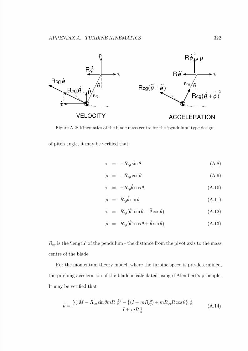
8/13/2019 Wholewhole
http://slidepdf.com/reader/full/wholewhole 347/396
APPENDIX A. TURBINE KINEMATICS 322
τ
ρ
Rcg
....ρ
....τ
....φ R
R........φ
VELOCITY ACCELERATION
....φ Rcg
....θ Rcg
θ
τ
ρ
Rcg θ
R....φ
2
........θRcg( )+φ
2
................θRcg( )+φ
Figure A.2: Kinematics of the blade mass centre for the ‘pendulum’ type design
of pitch angle, it may be verified that:
τ = −Rcg sin θ (A.8)
ρ = −Rcg cos θ (A.9)
τ = −Rcg θ cos θ (A.10)
ρ = Rcg θ sin θ (A.11)
τ = Rcg(θ2 sin θ − θ cos θ) (A.12)
ρ = Rcg(θ2 cos θ + θ sin θ) (A.13)
Rcg
is the ‘length’ of the pendulum - the distance from the pivot axis to the mass
centre of the blade.
For the momentum theory model, where the turbine speed is pre-determined,
the pitching acceleration of the blade is calculated using d’Alembert’s principle.
It may be verified that
¨θ =
M − Rcg sin θmR φ2 − (I + mR 2cg ) + mRcgR cos θ φ
I + mR 2cg (A.14)
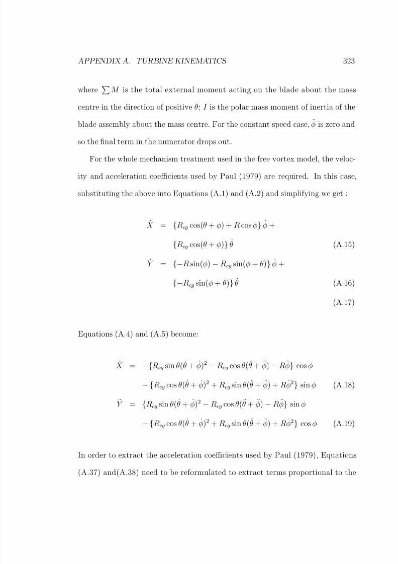
8/13/2019 Wholewhole
http://slidepdf.com/reader/full/wholewhole 348/396
APPENDIX A. TURBINE KINEMATICS 323
where M is the total external moment acting on the blade about the mass
centre in the direction of positive θ; I is the polar mass moment of inertia of the
blade assembly about the mass centre. For the constant speed case, φ is zero and
so the final term in the numerator drops out.
For the whole mechanism treatment used in the free vortex model, the veloc-
ity and acceleration coefficients used by Paul (1979) are required. In this case,
substituting the above into Equations (A.1) and (A.2) and simplifying we get :
X = Rcg cos(θ + φ) + R cos φ φ +
Rcg cos(θ + φ) θ (A.15)
Y = −R sin(φ) − Rcg sin(φ + θ) φ +
−Rcg sin(φ + θ) θ (A.16)
(A.17)
Equations (A.4) and (A.5) become:
X = −Rcg sin θ(θ + φ)2 − Rcg cos θ(θ + φ) − Rφ cos φ
− Rcg cos θ(θ + φ)2 + Rcg sin θ(θ + φ) + R φ2 sin φ (A.18)
Y = Rcg sin θ(θ + φ)2 − Rcg cos θ(θ + φ) − Rφ sin φ
− Rcg cos θ(θ + φ)2 + Rcg sin θ(θ + φ) + R φ2 cos φ (A.19)
In order to extract the acceleration coefficients used by Paul (1979), Equations
(A.37) and(A.38) need to be reformulated to extract terms proportional to the

8/13/2019 Wholewhole
http://slidepdf.com/reader/full/wholewhole 349/396
APPENDIX A. TURBINE KINEMATICS 324
generalised coordinate accelerations:
X = Rcg cos(θ + φ) + R cos φ φ +
Rcg cos(θ + φ) θ
−Rcg( φ + θ)2 sin(φ + θ) − R φ2 sin φ (A.20)
Y = −R sin(φ) − Rcg sin(φ + θ) φ +
−Rcg sin(φ + θ) θ
−Rcg( φ + θ)2 cos(φ + θ) − R φ2 cos φ (A.21)
The non-zero velocity coefficients for blade i are then:
U i0 = R cos φ + Rcg cos(φ + θ)
U ii = Rcg cos(φ + θ)
V i0 = −R sin(φ) − Rcg sin(φ + θ)
V ii = −Rcg sin(φ + θ) (A.22)
Equations (A.20) and (A.21) can then be seen to be:
X = U ii θ + U i0
φ + U
Y = V ii θ + V i0
φ + V (A.23)

8/13/2019 Wholewhole
http://slidepdf.com/reader/full/wholewhole 350/396
APPENDIX A. TURBINE KINEMATICS 325
where the acceleration coefficients, which contain centripetal and Coriolis acceler-
ation components, are:
U = −Rcg( φ + θ)2 sin(φ + θ) − R φ2 sin φ
V = −Rcg( φ + θ)2 cos(φ + θ) − R φ2 cos φ
A.2 Rolling Profile KinematicsThe derivation of the rolling profile shape for a desired moment-angle relationship
is described in Section 3.3.
d
y
θ
τ
ρ
r
........τ
........ρ
....ρ
....τ
r....φ
....φ R
d
y
θ
τ
ρ
r
r........φ
Vrel
....φ 2 Vrel
r....φ 2
R.... ....φ
VELOCITY ACCELERATION
R....φ
2
Figure A.3: Kinematics of the rolling profile design concept
The radial coordinate ρ is equal to the dimension y. According to Equation
(3.4) on page 60, y is defined in terms of the specified relationship between d and
θ:
∂y
∂θ = d(θ) (A.24)
giving:
y = ρ =
d dθ + y0 (A.25)

8/13/2019 Wholewhole
http://slidepdf.com/reader/full/wholewhole 351/396
APPENDIX A. TURBINE KINEMATICS 326
The τ coordinate is found by assuming no-slip rolling contact. Then τ is the
arc length from the initial contact point to the current contact point minus the
offset d. Labelling the arc length coordinate between the initial position (θ = 0)
and the contact point corresponding to pitch angle θ as s:
τ = s − d (A.26)
dy
θX
Y D
Crelative topoint D
p
q
δ
δθ
d
δy
δθ
d
y
Figure A.4: Rolling profile coordinate system, showing the infinitesimal displacementsof a point C at (d,y,θ) in terms of infinitesimal changes in the coordinates.
Figure A.4 shows the infinitesimal displacements of a point C in terms of in-
finitesimal changes in the coordinates d, y and θ. It can be seen that:
δs = δd + y δθ (A.27)

8/13/2019 Wholewhole
http://slidepdf.com/reader/full/wholewhole 352/396
APPENDIX A. TURBINE KINEMATICS 327
Accordingly,
s =
θ
0
dd
dΘ + y
dΘ
dΘ
dΘ
= d +
θ
0
y dΘ (A.28)
From Equations (A.26) and (A.28),
τ =
θ
0
y dΘ (A.29)
The relative velocities are then obtained by differentiation. From Equation(A.29):
τ = dτ
dθ
dθ
dt = yθ (A.30)
and from Equation (A.25):
ρ = dρ
dθ
dθ
dt = dθ (A.31)
Differentiating again to obtain accelerations:
τ = d2τ
dθ2θ2 +
dτ
dθθ
= d θ2 + y θ (A.32)
and
ρ = d2ρ
dθ2θ2 +
dρ
dθθ
= dd
dθθ2 + d θ (A.33)

8/13/2019 Wholewhole
http://slidepdf.com/reader/full/wholewhole 353/396
APPENDIX A. TURBINE KINEMATICS 328
For the single-degree-of-freedom treatment used in the momentum model, the
pitching acceleration is found for the instantaneous values of the pitch and pitching
velocity θ and θ and the turbine speed and acceleration φ and φ. It may be verified
using Figure A.3 that
θ =
M − [I − mτ d + ρ(R − ρ)] φ − mA
I + m(d2 + ρ2) (A.34)
where
M = M + F ρd + F τ ρ
A =
d(ρ +
dd
dθ)θ2 − τ ρ − d(R − ρ) φ2
As in Section A.1, M is the external moment about the mass centre. F ρ and F τ
are the radial and tangential components of the external aerodynamic force on the
blade.
In this case, Equations (A.1) and (A.2) become:
X = (−ρ cos φ − d sin φ) θ + ((R − ρ)cos φ + τ sin φ) φ (A.35)
Y = (ρ sin φ − d cos φ) θ + ((ρ − R)sin φ + τ cos φ) φ (A.36)
Equations (A.4) and (A.5) become:
X = (R − ρ)φ − (dθ2 + ρθ) − 2dθ φ − τ φ2 cos φ
+ τ φ − (dd
dθθ2 + dθ) + 2τ φ − (R − ρ) φ2 sin φ (A.37)
Y = τ φ − (
dd
dθ θ2
+ dθ) + 2τ φ − (R − ρ) φ2
cos φ
− (R − ρ)φ − (dθ2 + ρθ) − 2dθ φ − τ φ2 sin φ (A.38)

8/13/2019 Wholewhole
http://slidepdf.com/reader/full/wholewhole 354/396
APPENDIX A. TURBINE KINEMATICS 329
In order to extract the acceleration coefficients used by Paul (1979), Equations
(A.37) and(A.38) need to be reformulated to extract terms proportional to the
generalised coordinate accelerations:
X = (−ρ cos φ − d sin φ) θ + ((R − ρ)cos φ + τ sin φ) φ
+ (−d cos φ − dd
dθ sin φ) θ2 + (−2d cos φ + 2ρ sin φ) φθ
+ (ρ − R)sin φ + τ cos φ ˙φ
2
(A.39)
Y = (ρ sin φ − d cos φ) θ + ((ρ − R)sin φ + τ cos φ) φ
+ (d sin φ − dd
dθ cos φ) θ2 + (2d sin φ + 2ρ cos φ) φθ
+ (ρ − R)cos φ − τ sin φ φ2 (A.40)
The non-zero velocity coefficients for blade i are then:
U i0 = (R − ρ)cos φ + τ sin φ
U ii = −ρ cos φ − d sin φ
V i0 = (ρ − R)sin φ + τ cos φ
V ii = ρ sin φ − d cos φ (A.41)
Equations (A.39) and (A.40) can then be seen to be:
X = U ii θ + U i0
φ + U
Y = V ii θ + V i0
φ + V (A.42)

8/13/2019 Wholewhole
http://slidepdf.com/reader/full/wholewhole 355/396
APPENDIX A. TURBINE KINEMATICS 330
where the acceleration coefficients are:
U = (−d cos φ − dd
dθ sin φ) θ2 + (−2d cos φ + 2ρ sin φ) φθ
+ (ρ − R)sin φ + τ cos φ φ2
V = (d sin φ − dd
dθ cos φ) θ2 + (2d sin φ + 2ρ cos φ) φθ
+ (ρ − R)cos φ − τ sin φ φ2 (A.43)
If the specified relationship between d and θ is analytic, differentiable and
integrable, then the positions, velocities and accelerations derived above may be
found analytically.
For example, for a simple circular profile or radius R p and centre of gravity
located at radius Rcg from the centre of curvature, d = Rcg sin θ and y = R p −
Rcg cos θ. We then get:
τ =
θ
0
y dΘ = R pθ − q sin θ
ρ = y = R p − Rcg cos θ
τ = yθ = (R p − Rcg cos θ)θ
ρ = dθ = (Rcg sin θ)θ
τ = d θ2 + y θ = (Rcg sin θ)θ2 + R p − (Rcg cos θ)θ
ρ = dd
dθθ2 + d θ = (Rcg cos θ)θ2 + (Rcg sin θ)θ
If d is not defined analytically, then the above quantities must be determined
numerically. Note that it may be defined in a piecewise analytical fashion also.

8/13/2019 Wholewhole
http://slidepdf.com/reader/full/wholewhole 356/396
APPENDIX A. TURBINE KINEMATICS 331
Equation A.34, giving the pitching acceleration for known position, velocity
and rotor acceleration, becomes
θ =
M −
I − mRR p − R2
cg − R2 p + R pθRcg sin θ − (R − 2R p)Rcg cos θ
φ − mA
I + m(R2cg + R2
p − 2RRcg cos θ)
(A.44)
where
M = M + F ρ(Rcg sin θ) + F τ (R p − Rcg cos θ)
A =
(R pRcg sin θ)θ2 − R2 pθ − R pθRcg cos θ − RRcg sin θ φ2
Note that if R p is set to zero, the situation reverts to that for a pendulum of
length Rcg. It may be checked that Equation A.44 reverts to Equation A.14.
A.3 Kinematics of the Kirke-Lazuaskas Design
In the Kirke-Lazauskas design (Kirke and Lazauskas, 1992; Kirke, 1998), a separate
stabiliser mass that is free to slide radially along the support arm provides the
restoring moment. Unlike other designs, the magnitude of the restoring moment is
independent of the pitch angle, and depends only on the offset between pivot axis
and the point of contact between stabiliser mass and blade (labelled af and ar in
Figure A.5. The design allows the restoring moment to be different for positive
and negative pitch angles.
Referring to Figure A.6, the restoring moment M r is given by
M r = msρ + (R − ρ) φ2 af for θ > 0
= −msρ + (R − ρ) ˙φ
2
ar for θ < 0 (A.45)
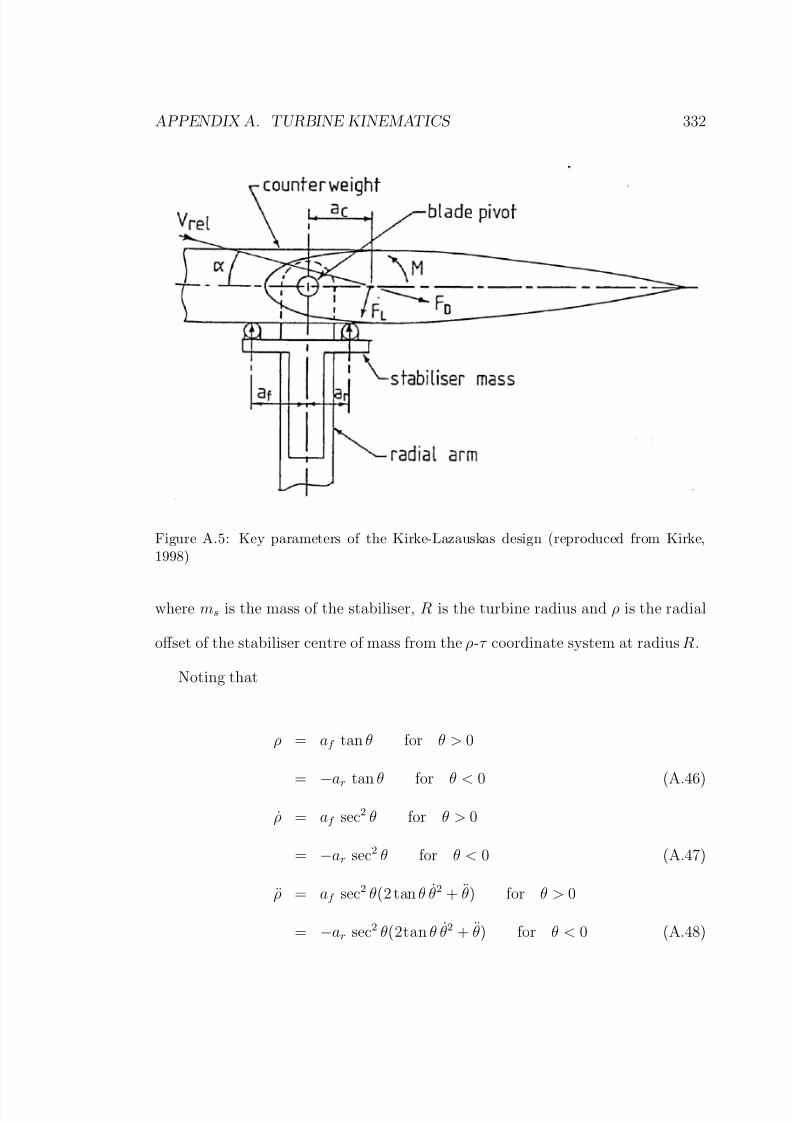
8/13/2019 Wholewhole
http://slidepdf.com/reader/full/wholewhole 357/396
APPENDIX A. TURBINE KINEMATICS 332
Figure A.5: Key parameters of the Kirke-Lazauskas design (reproduced from Kirke,1998)
where ms is the mass of the stabiliser, R is the turbine radius and ρ is the radial
offset of the stabiliser centre of mass from the ρ-τ coordinate system at radius R.
Noting that
ρ = af tan θ for θ > 0
= −ar tan θ for θ < 0 (A.46)
ρ = af sec2 θ for θ > 0
= −ar sec2 θ for θ < 0 (A.47)
ρ = af sec2 θ(2 tan θ θ2 + θ) for θ > 0
= −ar sec2 θ(2tan θ θ2 + θ) for θ < 0 (A.48)

8/13/2019 Wholewhole
http://slidepdf.com/reader/full/wholewhole 358/396
APPENDIX A. TURBINE KINEMATICS 333
2....φ
....ρ
2
)+ (R-....φ
........ρ ρ
)(R-........φ ρ
τ
ρ
.... ....φ
θ........
+........
φ
R........φ
R2....
φ
m
ms
θ
....φ
Figure A.6: Acceleration components of the blade and stabiliser mass for the Kirke-Lazauskas design (Kirke, 1998)
Equation (A.49) becomes
M r = msaf sec2 θ(2tan(θ) θ2 + θ) + (R − af tan θ) φ2 af for θ > 0
= −ms−ar sec2 θ(2 tan(θ) θ2 + θ) + (R + ar tan θ) φ2 ar for θ < 0
(A.49)
Using d’Alembert’s principle, the pitching acceleration is found to be:
θ =
M − M r − φ
I

8/13/2019 Wholewhole
http://slidepdf.com/reader/full/wholewhole 359/396
APPENDIX A. TURBINE KINEMATICS 334
which becomes:
θ =
M − msaf sec2 θ(2tan(θ) θ2) + (R − af tan θ) φ2 af − φ
I + ms(af sec θ)2 for θ > 0
=
M + ms−ar sec2 θ(2tan(θ) θ2) + (R + ar tan θ) φ2 ar − φ
I + ms(ar sec θ)2 for θ < 0
(A.50)
where
M is the total aerodynamic moment about the pivot axis and I is the
polar mass moment of inertia about the pivot axis.
Note that there is a step change in the restoring moment across θ = 0. When
θ = 0, the restoring moment may vary to match the disturbing aerodynamic
moment up to a magnitude equal to that given by Equation A.49.
It is very difficult to properly model the motion of the blade pitching through
θ = 0. Because the stabilising mass is asked to change directions instantaneously,
the real force will be determined by the compressibility and damping of the contact
regions. This complexity is neglected in the present analysis.
It should also be noted that the radial movement of the stabiliser mass results
in inertial moment and tangential reactions on the rotor. From Figure A.6 it may
be seen that the tangential reaction, decelerating the rotor, is given by:
Rτ = ms(R − ρ)φ − 2 φρ
= ms(R − af tan θ)φ − 2 φθaf sec2 θ for θ > 0
= ms(R + ar tan θ)φ + 2 φθar sec2 θ for θ < 0

8/13/2019 Wholewhole
http://slidepdf.com/reader/full/wholewhole 360/396
APPENDIX A. TURBINE KINEMATICS 335
The inertial moment reaction, also decelerating the rotor, is:
M reac = I sφ − msaf sec2 θ(2tan(θ) θ2 + θ) + (R − af tan θ) φ2 for θ > 0
= I sφ + ms−ar sec2 θ(2 tan(θ) θ2 + θ) + (R + ar tan θ) φ2 for θ < 0
(A.51)
These reactions affect the instantaneous turbine torque, just as inertial reac-
tions affect the torque for the pendulum and rolling contact designs.
A.4 Comparison of Blade Responsiveness for Different Designs
The three designs analysed above all rely on inertial forces to produce the restoring
moment on the blade. For the same blade and counterweight, each design results
in a different ‘effective moment of inertia’ for the blade assembly, resulting in
different dynamic response to aerodynamic driving forces.
Compare the expressions for the pitching acceleration given a values of external
driving moment, blade position and velocity and turbine velocity and acceleration,
for the three designs:
¨
θ =
F tRcg + M − Rcg sin θmR φ2 − (I + mR 2cg) + mRcgR cos θ φ
I + mR 2cg
for the pendulum type (A.14)
θ =
M − [I − mτ d + ρ(R − ρ)] φ − mA
I + m(d2 + ρ2)
for the rolling profile (A.34)
θ =
M − msaf sec2 θ(2 tan(θ) θ2) + (R − af tan θ) φ2 af − φ
I + ms(af sec θ)2 for θ > 0
for the Kirke-Lazauskas design (A.50)

8/13/2019 Wholewhole
http://slidepdf.com/reader/full/wholewhole 361/396
APPENDIX A. TURBINE KINEMATICS 336
The denominators of the three expressions may be regarded as the effective
mass moments of inertia for the three designs. The pendulum type is simply the
moment of inertia about the pivot axis using the translation of axes theorem.
For the rolling profile, the relevant moment of inertia is that about the con-
tact point. The moment of inertia therefore changes with the pitch angle, and is
minimum at zero.
For the Kirke-Lazauskas design, the effective moment of inertia also changeswith pitch angle, and may be seen to be that equivalent to lumping the stabiliser
mass at the contact point.

8/13/2019 Wholewhole
http://slidepdf.com/reader/full/wholewhole 362/396
Appendix B
Dynamic Stall Models
Details of the Boeing-Vertol dynamic stall method, including modifications sug-
gested by Cardona (1984), and the MIT model as modified by Noll and Ham (1982)
are given below.
B.1 Boeing-Vertol (Gormont) Dynamic Stall Model
The Boeing-Vertol method is not a full unsteady aerodynamics model as it does
not modify the aerodynamic forces on an aerofoil pitching at angles below static
stall. It models the delayed stall and increased lift observed in pitching aerofoil
experiments. Delayed stall is handled by using static lift, drag and moment co-
efficient look-up tables with a modified angle of attack. The empirical angle of
attack modification is derived from wind tunnel data on oscillating aerofoils. The
modified angle of attack is a function of the square root of a dimensionless pitch
rate parameter:
αm = αB − γK 1
cαB
2W
1/2
sign(αB) (B.1)
where αm is the modified angle, αB is the geometric angle of attack, c is the
blade chord, W is the relative flow velocity.
The drag and moment coefficients based on this modified angle of attack are
found directly from the static look-up table, while the lift coefficient is increased
337

8/13/2019 Wholewhole
http://slidepdf.com/reader/full/wholewhole 363/396
APPENDIX B. DYNAMIC STALL MODELS 338
by a factor proportional to the angle of attack modification:
C L = C L(αm)
αm
αB − α0
C D = C D(αm) (B.2)
C M = C M (αm)
where α0 is the angle of attack at which lift is zero (0 for a symmetrical section).
The gamma functions are also empirically derived and are functions of the
blade thickness to chord ratio.
γ L = 1.4 − 6
0.06 −
t
c
γ D = 1 − 2.5
0.06 −
t
c
(B.3)
γ M = γ D
K 1 changes with the sign of the rate of change of angle of attack and is specified
as 1.0 when a is increasing in magnitude and 0.5 when it is decreasing in magnitude.
Paraschivoiu and Allet (1988) state that the model is especially applicable to
thin aerofoils (t/c < 12%) and is not suited to deep stall (α > αstatic stall + 5).
Strickland et al. (1981) applied the model when the angle of attack exceeds the
static stall angle or when the angle is decreasing having been above stall. This
models the hysteresis observed oscillating aerofoil experiments.
B.2 MIT Dynamic Stall Model
The MIT dynamic stall model similarly does not deal with dynamic effects in the
attached flow case, only with the delay of stall under dynamic conditions. In the
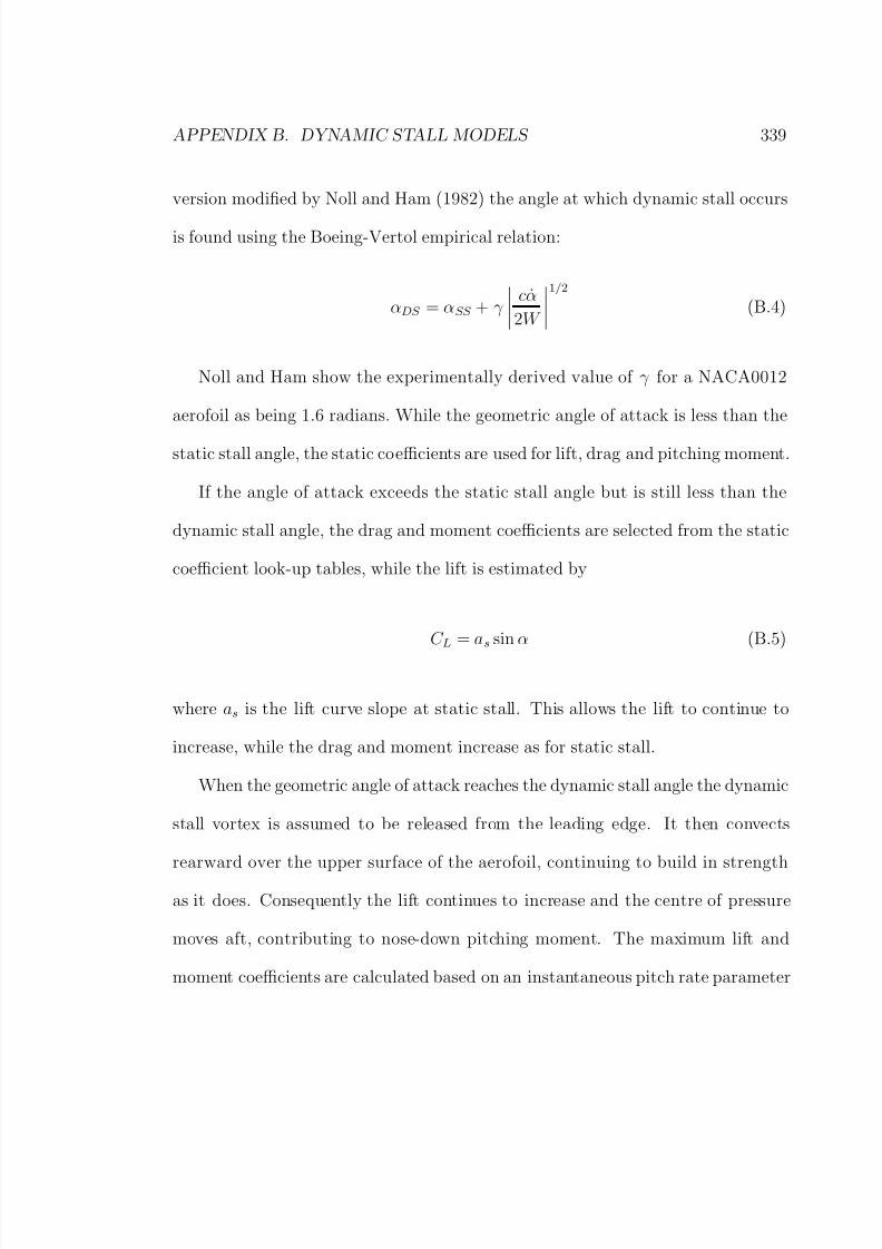
8/13/2019 Wholewhole
http://slidepdf.com/reader/full/wholewhole 364/396
APPENDIX B. DYNAMIC STALL MODELS 339
version modified by Noll and Ham (1982) the angle at which dynamic stall occurs
is found using the Boeing-Vertol empirical relation:
αDS = αSS + γ
cα
2W
1/2
(B.4)
Noll and Ham show the experimentally derived value of γ for a NACA0012
aerofoil as being 1.6 radians. While the geometric angle of attack is less than the
static stall angle, the static coefficients are used for lift, drag and pitching moment.
If the angle of attack exceeds the static stall angle but is still less than the
dynamic stall angle, the drag and moment coefficients are selected from the static
coefficient look-up tables, while the lift is estimated by
C L = as sin α (B.5)
where as is the lift curve slope at static stall. This allows the lift to continue to
increase, while the drag and moment increase as for static stall.
When the geometric angle of attack reaches the dynamic stall angle the dynamic
stall vortex is assumed to be released from the leading edge. It then convects
rearward over the upper surface of the aerofoil, continuing to build in strength
as it does. Consequently the lift continues to increase and the centre of pressure
moves aft, contributing to nose-down pitching moment. The maximum lift and
moment coefficients are calculated based on an instantaneous pitch rate parameter

8/13/2019 Wholewhole
http://slidepdf.com/reader/full/wholewhole 365/396
APPENDIX B. DYNAMIC STALL MODELS 340
from an empirically derived relation:
C Lmax = 1.0 + 40.0
cα
W
if 0 ≤
cα
W
≤ 0.05
= 3.0 otherwise (B.6)
C M max = −0.15 if 0 ≤
cα
W
≤ 0.02
= −0.15 − 21.0
cα
W
− 0.02
if 0.02 <
cα
W
≤ 0.05
= −0.78 otherwise (B.7)
The lift coefficient continues to be calculated from Equation B.5 until it reaches
the maximum value. It is assumed that the maximum lift occurs when the dynamic
stall vortex reaches the midchord, while the maximum pitching moment occurs
when it reaches the 3/4 chord position. Pitching moment about the quarter chord
in this region is calculated on the basis of the position of the centre of pressure.
C M = −C N (X CP − 0.25) (B.8)
where X CP is the distance (in chords) of the centre of pressure from the leading
edge. The rearward velocity of the centre of pressure is assumed to be constant,
and the position, prior to reaching C Lmax, is given by:
X CP = (t − tDS )V
4c + 0.25 (B.9)
and subsequent to reaching C Lmax by:
X CP = (t − tL)(0.75 − X CP L)2V
c + X CP L (B.10)
8/13/2019 Wholewhole
http://slidepdf.com/reader/full/wholewhole 366/396
APPENDIX B. DYNAMIC STALL MODELS 341
Once the lift and moment coefficients reach their pre-determined maximum values,
according to the MIT model they are held at this level until the peak angle of
attack is reached. Only after this point do the lift and moment begin to decay
exponentially back to the static stall values.
C L = (C Lmax − C LSS )e−(ψ−ψ0)2R/c + C LSS (B.11)
C M = (C M max
− C M SS
)e−(ψ−ψ0)2R/2.5c + C M SS
(B.12)
where time has been expressed in terms of the azimuth angle specifically for Dar-
rieus turbines. ψ is the current azimuth and ψ0 is the azimuth at the start of
decay.
This part of the model is problematic. Derived from oscillating aerofoil wind
tunnel test data and developed for helicopter applications, it is not suitable for
studying the low speed performance Darrieus turbines in this form. At low tip
speed ratios the amplitude of the angle of attack oscillations may be very large (up
to 90) and it is not plausible that this peak lift and moment would be maintained
for so long after the inception of dynamic stall. Worse, at tips speed ratios less
than one, the angle of attack does not oscillate but continuously decreases, the
relative wind orbiting the blade with each revolution of the rotor.
Thus some alternative criterion is required for the commencement of the decay
of lift. The passage of the dynamic stall vortex beyond the trailing edge of the
aerofoil would seem to be a reasonable criterion, as this is used in the indicial
Beddoes-Leishman model. Since it has already been assumed that the velocity
of the vortex is constant and that the maximum lift occurs when it reaches the
midchord, the time of arrival at the trailing edge is simply twice the time after

8/13/2019 Wholewhole
http://slidepdf.com/reader/full/wholewhole 367/396
APPENDIX B. DYNAMIC STALL MODELS 342
the start of dynamic stall to the attainment of maximum lift. At this point decay
begins, whether or not the peak angle of attack has been reached.
The decay of lift and moment coefficients towards the static stall values is also
not compatible with a monotonic increase in the magnitude of angle of attack.
Accordingly, the coefficients are made to decay towards the static value at the
current angle of attack. That is:
C L = [C Lmax − C Lstatic(α)] e−(ψ−ψ0)2R/c + C Lstatic(α) (B.13)
C M = [C M max − C M static(α)] e−(ψ−ψ0)2R/2.5c + C M static(α) (B.14)
In this way, as the blade continues into deep stall, the lift and moment coefficients
approach the static values at high angles of attack, effectively ‘turning off’ the
dynamic stall model.
If angle of attack starts to decrease before peak lift is attained, decay begins
immediately from the currently attained lift and moment values.
The exponential decay continues until the angle of attack drops to below the
static stall angle once more and attached flow is assumed to resume. Paraschivoiu
and Allet (1988) claim that the MIT model fails to predict the delayed reattach-
ment of flow, to angles well below static stall, that is observed in experiments.
Above the dynamic stall angle and during the exponential decay of coefficients,
Noll and Ham calculate the drag by
C D = C L tan α (B.15)
The problem with this relation is that while it produces plausible values for the
drag coefficient, for a blade at zero-pitch on a Darrieus turbine, the tangential
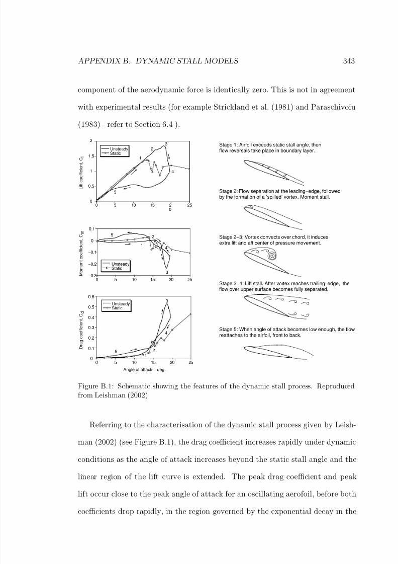
8/13/2019 Wholewhole
http://slidepdf.com/reader/full/wholewhole 368/396
APPENDIX B. DYNAMIC STALL MODELS 343
component of the aerodynamic force is identically zero. This is not in agreement
with experimental results (for example Strickland et al. (1981) and Paraschivoiu
(1983) - refer to Section 6.4 ).
Stage 1: Airfoil exceeds static stall angle, thenflow reversals take place in boundary layer.
Stage 2: Flow separation at the leading−edge, followed
by the formation of a ’spilled’ vortex. Moment stall.
Stage 2−3: Vortex convects over chord, it inducesextra lift and aft center of pressure movement.
Stage 3−4: Lift stall. After vortex reaches trailing−edge, theflow over upper surface becomes fully separated.
Stage 5: When angle of attack becomes low enough, the flowreattaches to the airfoil, front to back.
−0.3
−0.2
−0.1
0
0.1
0 5 10 15 20 25
UnsteadyStatic
1
2
3
4
5
0
0.5
1
1.5
2
0 5 10 15 20
25
UnsteadyStatic
1
23
4
5
0
0.1
0.2
0.3
0.4
0.5
0.6
0 5 10 15 20 25
UnsteadyStatic
Angle of attack − deg.
3
4
251
L i f t c o e f f i c i e n t , C l
M o m e n t c o e f f i c i e n t , C m
D r a g c o e f f i c i e n t , C d
Figure B.1: Schematic showing the features of the dynamic stall process. Reproduced
from Leishman (2002)
Referring to the characterisation of the dynamic stall process given by Leish-
man (2002) (see Figure B.1), the drag coefficient increases rapidly under dynamic
conditions as the angle of attack increases beyond the static stall angle and the
linear region of the lift curve is extended. The peak drag coefficient and peak
lift occur close to the peak angle of attack for an oscillating aerofoil, before both
coefficients drop rapidly, in the region governed by the exponential decay in the

8/13/2019 Wholewhole
http://slidepdf.com/reader/full/wholewhole 369/396
APPENDIX B. DYNAMIC STALL MODELS 344
MIT model. These features are confirmed by the experimental work of Laneville
and Vittecoq (1986) and of Lorber and Carta (1988).
Instead of using Equation B.15 therefore, the drag for the period after the
dynamic stall angle (determined from Equation B.4) is reached but before lift
coefficient decay begins is calculated here by:
C D = C D(α)|α/αDS | (B.16)
The normal static increase in drag associated with angles of attack above static
stall is exaggerated by scaling the static coefficient by the ratio of the current angle
to the angle at which dynamic stall began.
Once the decay of the lift coefficient begins, the drag coefficient is linked to the
lift coefficient using the expression:
C D = C Dstatic(α)|C L/C Lstatic(α)| (B.17)
C L is calculated using Equation B.11. The drag coefficient is thus naturally linked
to the decay time constant for the lift coefficient and decays with it towards the
static value at the current angle of attack.
While the above modifications to the MIT method are to some extent arbitrary
in their specific form, they are consistent with the documented features of dynamic
stall and address aspects of the model that are clearly inappropriate for application
to the starting behaviour of Darrieus turbines. The modifications were settled on
because they provided the best agreement with available experimental data on
Darrieus blade forces. Validation against this data is discussed in Section 6.4.

8/13/2019 Wholewhole
http://slidepdf.com/reader/full/wholewhole 370/396
Appendix C
Calculation of the prototype turbine drag coefficient
Calculations of the torque lost to bearing and brake friction and parasitic aerody-
namic drag for the prototype turbine are presented.
Drag losses were estimated by measuring the decay of turbine speed in still
air. As no motor was provided to accelerate the turbine, these measurements had
to be conducted at the end of wind tunnel test runs by reducing the wind speed
to zero and allowing the turbine to coast to rest. Data from five separate runs is
shown in Figure C.1.
The total torque decelerating the turbine was estimated by calculating the
deceleration by numerical differentiation. To reduce scatter in the results, the
data was thinned, taking speed values every 5 seconds. A cubic spline was fitted
through the values and the slopes at the data points used as the acceleration values.
The acceleration was multiplied by the total moment of inertia of the turbine to
give the torque. Torque is plotted as a function of speed for these five runs in
Figure C.2.
A curve was then fitted through the torque-speed data. The curve fitting was
function was chosen to be of the form
T = Aω2 + B (C.1)
345

8/13/2019 Wholewhole
http://slidepdf.com/reader/full/wholewhole 371/396
APPENDIX C. TURBINE DRAG 346
0
20
40
60
80
100
120
0 50 100 150 200 250
Time [s]
T
u r b i n e S p e e d [ r p m ]
Figure C.1: Measured still air speed decay for five runs.
-3
-2.5
-2
-1.5
-1
-0.5
0
0 2 4 6 8 10 12
Speed [rad/s]
T o r q u e [ N m ]
Data
T = -0.0187s2 - 0.215
I = 21.388 kgm2
Figure C.2: Torque found by numerical differentiation.

8/13/2019 Wholewhole
http://slidepdf.com/reader/full/wholewhole 372/396
APPENDIX C. TURBINE DRAG 347
This assumes that the total resistance is composed of aerodynamic drag, which is
assumed proportional to the square of the turbine speed, and dry friction, which
is independent of speed. The values of A and B for this data were found to be
0.0187 and 0.215 respectively. The curve provides a good fit to the data, except for
speeds below approximately 1 rad/s, where the drag appears to increase slightly.
This measured drag includes that from the blades themselves, as well as the
non-working parts of the turbine. For application to the mathematical models, thedrag contributed by the blades was subtracted from the total, as this component
is accounted for by the blade section drag coefficient data.
The still air drag due to the blades alone was calculated as:
T blades = N b1
2 C d0 ρ L c R (Rω)2 (C.2)
where N b is the number of blades, C d0 is the zero incidence drag coefficient, ρ is
the air density, L is the length of the blades, c is the blade chord, R is the turbine
radius and ω is the turbine speed.
The blade drag coefficient is defined as:
Ablades = T blade/ω2
= N b1
2 C d0 ρ L c R3
= 3 x 0.5 x 0.02 x 1.2 x 1.3 x 0.15 x 0.873
= 0.0046 (C.3)
This coefficient is subtracted from the total aerodynamic drag coefficient mea-
sured for the turbine above. In the momentum and vortex mathematical models,

8/13/2019 Wholewhole
http://slidepdf.com/reader/full/wholewhole 373/396
APPENDIX C. TURBINE DRAG 348
a retarding torque calculated by
T drag = (A − Ablades) ω2 + B
= (0.0187 − 0.0046) ω2 + 0.215
= 0.0141 ω2 + 0.215 Nm (C.4)
is subtracted from the raw torque at turbine speed ω rad/s.

8/13/2019 Wholewhole
http://slidepdf.com/reader/full/wholewhole 374/396
Appendix D
Aerofoil aerodynamic data
The following data was used for the NACA0018 profile used in the mathematical
models. It was still available as at 3/10/2002 online athttp://www.maths.adelaide.edu.au/Applied/llazausk/aero/foil/foil.htm. Lift and
drag coefficient data is plotted in Figure D.1.
---------------------------------------------------------------------
AIRFOIL: NACA 0018
DATA: Lift Coefficients
---------------------------------------------------------------------
ORIGINAL SOURCE: Sheldahl, R. E. and Klimas, P. C., Aerodynamic
Characteristics of Seven Airfoil Sections Through
180 Degrees Angle of Attack for Use in Aerodynamic
Analysis of Vertical Axis Wind Turbines, SAND80-2114,
March 1981, Sandia National Laboratories, Albuquerque,
New Mexico.
NOTES: The data herein were synthesised from a combination of
experimental results and computer calculations.
The original report contains data for lower Reynolds numbers
than contained herein, but there are some anomalies, in
particular with CL at small angles of attack.
Data extended to 360 degrees of attack and glaring anomalies
corrected by L. Lazauskas. All deviations from the original
are due to L. Lazauskas.
Please refer to the original report for more details.
349

8/13/2019 Wholewhole
http://slidepdf.com/reader/full/wholewhole 375/396
APPENDIX D. AEROFOIL DATA 350
------------------------------------------------------------------------
Lift Coefficient
-------------------------------- REYNOLDS NUMBER -----------------------
ALPHA 40000 80000 160000 360000 700000 1000000 2000000 5000000
------------------------------------------------------------------------
0 0.0000 0.0000 0.0000 0.0000 0.0000 0.0000 0.0000 0.0000
1 0.0936 0.0889 0.1100 0.1100 0.1100 0.1100 0.1100 0.1100
2 0.1833 0.1935 0.2200 0.2200 0.2200 0.2200 0.2200 0.2200
3 0.2688 0.2924 0.3088 0.3300 0.3300 0.3300 0.3300 0.3300
4 0.3495 0.3880 0.4114 0.4400 0.4400 0.4400 0.4400 0.4400
5 0.4117 0.4753 0.5068 0.5240 0.5500 0.5500 0.5500 0.5500
6 0.4573 0.5615 0.5960 0.6228 0.6328 0.6600 0.6600 0.6600
7 0.4758 0.6224 0.6724 0.7100 0.7291 0.7362 0.7449 0.7700
8 0.4428 0.6589 0.7373 0.7879 0.8156 0.8256 0.8439 0.8538
9 0.3544 0.6606 0.7781 0.8526 0.8904 0.9067 0.9314 0.9525
10 0.2108 0.6248 0.7949 0.8983 0.9541 0.9751 1.0111 1.0404
11 0.1124 0.5531 0.7852 0.9249 0.9973 1.0284 1.0772 1.1211
12 0.0139 0.4408 0.7488 0.9279 1.0245 1.0664 1.1296 1.1884
13 0.0314 0.3332 0.6923 0.9104 1.0289 1.0804 1.1662 1.2430
14 0.0489 0.2256 0.6237 0.8803 1.0175 1.0793 1.1813 1.2808
15 0.0889 0.2142 0.5567 0.8405 0.9938 1.0624 1.1813 1.3004
16 0.1287 0.2027 0.4896 0.8007 0.9648 1.0402 1.1695 1.3067
17 0.1758 0.2315 0.4549 0.7663 0.9399 1.0181 1.1550 1.3038
18 0.2228 0.2603 0.4202 0.7319 0.9150 0.9959 1.1383 1.2960
19 0.2732 0.3038 0.4292 0.7158 0.9014 0.9833 1.1278 1.2853
20 0.3236 0.3472 0.4382 0.6997 0.8877 0.9707 1.1172 1.2768
21 0.3751 0.3951 0.4704 0.7024 0.8872 0.9702 1.1150 1.2741
22 0.4265 0.4430 0.5026 0.7050 0.8867 0.9696 1.1127 1.2714
25 0.5840 0.5963 0.6321 0.7724 0.9326 1.0107 1.1468 1.2925
30 0.8550 0.8550 0.8550 0.8550 0.8550 0.8550 0.8550 0.8550
35 0.9800 0.9800 0.9800 0.9800 0.9800 0.9800 0.9800 0.9800
40 1.0350 1.0350 1.0350 1.0350 1.0350 1.0350 1.0350 1.0350
45 1.0500 1.0500 1.0500 1.0500 1.0500 1.0500 1.0500 1.0500
50 1.0200 1.0200 1.0200 1.0200 1.0200 1.0200 1.0200 1.0200
55 0.9550 0.9550 0.9550 0.9550 0.9550 0.9550 0.9550 0.9550
60 0.8750 0.8750 0.8750 0.8750 0.8750 0.8750 0.8750 0.875065 0.7600 0.7600 0.7600 0.7600 0.7600 0.7600 0.7600 0.7600
70 0.6300 0.6300 0.6300 0.6300 0.6300 0.6300 0.6300 0.6300

8/13/2019 Wholewhole
http://slidepdf.com/reader/full/wholewhole 376/396
APPENDIX D. AEROFOIL DATA 351
75 0.5000 0.5000 0.5000 0.5000 0.5000 0.5000 0.5000 0.5000
80 0.3650 0.3650 0.3650 0.3650 0.3650 0.3650 0.3650 0.3650
85 0.2300 0.2300 0.2300 0.2300 0.2300 0.2300 0.2300 0.2300
90 0.0900 0.0900 0.0900 0.0900 0.0900 0.0900 0.0900 0.0900
95 -0.0500 -0.0500 -0.0500 -0.0500 -0.0500 -0.0500 -0.0500 -0.0500
100 -0.1850 -0.1850 -0.1850 -0.1850 -0.1850 -0.1850 -0.1850 -0.1850
105 -0.3200 -0.3200 -0.3200 -0.3200 -0.3200 -0.3200 -0.3200 -0.3200
110 -0.4500 -0.4500 -0.4500 -0.4500 -0.4500 -0.4500 -0.4500 -0.4500
115 -0.5750 -0.5750 -0.5750 -0.5750 -0.5750 -0.5750 -0.5750 -0.5750
120 -0.6700 -0.6700 -0.6700 -0.6700 -0.6700 -0.6700 -0.6700 -0.6700
125 -0.7600 -0.7600 -0.7600 -0.7600 -0.7600 -0.7600 -0.7600 -0.7600
130 -0.8500 -0.8500 -0.8500 -0.8500 -0.8500 -0.8500 -0.8500 -0.8500
135 -0.9300 -0.9300 -0.9300 -0.9300 -0.9300 -0.9300 -0.9300 -0.9300
140 -0.9800 -0.9800 -0.9800 -0.9800 -0.9800 -0.9800 -0.9800 -0.9800
145 -0.9000 -0.9000 -0.9000 -0.9000 -0.9000 -0.9000 -0.9000 -0.9000
150 -0.7700 -0.7700 -0.7700 -0.7700 -0.7700 -0.7700 -0.7700 -0.7700
155 -0.6700 -0.6700 -0.6700 -0.6700 -0.6700 -0.6700 -0.6700 -0.6700
160 -0.6350 -0.6350 -0.6350 -0.6350 -0.6350 -0.6350 -0.6350 -0.6350
165 -0.6800 -0.6800 -0.6800 -0.6800 -0.6800 -0.6800 -0.6800 -0.6800
170 -0.8500 -0.8500 -0.8500 -0.8500 -0.8500 -0.8500 -0.8500 -0.8500
175 -0.6600 -0.6600 -0.6600 -0.6600 -0.6600 -0.6600 -0.6600 -0.6600
180 0.0000 0.0000 0.0000 0.0000 0.0000 0.0000 0.0000 0.0000
185 0.6600 0.6600 0.6600 0.6600 0.6600 0.6600 0.6600 0.6600
190 0.8500 0.8500 0.8500 0.8500 0.8500 0.8500 0.8500 0.8500
195 0.6800 0.6800 0.6800 0.6800 0.6800 0.6800 0.6800 0.6800
200 0.6350 0.6350 0.6350 0.6350 0.6350 0.6350 0.6350 0.6350
205 0.6700 0.6700 0.6700 0.6700 0.6700 0.6700 0.6700 0.6700
210 0.7700 0.7700 0.7700 0.7700 0.7700 0.7700 0.7700 0.7700
215 0.9000 0.9000 0.9000 0.9000 0.9000 0.9000 0.9000 0.9000
220 0.9800 0.9800 0.9800 0.9800 0.9800 0.9800 0.9800 0.9800
225 0.9300 0.9300 0.9300 0.9300 0.9300 0.9300 0.9300 0.9300
230 0.8500 0.8500 0.8500 0.8500 0.8500 0.8500 0.8500 0.8500
235 0.7600 0.7600 0.7600 0.7600 0.7600 0.7600 0.7600 0.7600
240 0.6700 0.6700 0.6700 0.6700 0.6700 0.6700 0.6700 0.6700
245 0.5750 0.5750 0.5750 0.5750 0.5750 0.5750 0.5750 0.5750
250 0.4500 0.4500 0.4500 0.4500 0.4500 0.4500 0.4500 0.4500
255 0.3200 0.3200 0.3200 0.3200 0.3200 0.3200 0.3200 0.3200260 0.1850 0.1850 0.1850 0.1850 0.1850 0.1850 0.1850 0.1850
265 0.0500 0.0500 0.0500 0.0500 0.0500 0.0500 0.0500 0.0500

8/13/2019 Wholewhole
http://slidepdf.com/reader/full/wholewhole 377/396
APPENDIX D. AEROFOIL DATA 352
270 -0.0900 -0.0900 -0.0900 -0.0900 -0.0900 -0.0900 -0.0900 -0.0900
275 -0.2300 -0.2300 -0.2300 -0.2300 -0.2300 -0.2300 -0.2300 -0.2300
280 -0.3650 -0.3650 -0.3650 -0.3650 -0.3650 -0.3650 -0.3650 -0.3650
285 -0.5000 -0.5000 -0.5000 -0.5000 -0.5000 -0.5000 -0.5000 -0.5000
290 -0.6300 -0.6300 -0.6300 -0.6300 -0.6300 -0.6300 -0.6300 -0.6300
295 -0.7600 -0.7600 -0.7600 -0.7600 -0.7600 -0.7600 -0.7600 -0.7600
300 -0.8750 -0.8750 -0.8750 -0.8750 -0.8750 -0.8750 -0.8750 -0.8750
305 -0.9550 -0.9550 -0.9550 -0.9550 -0.9550 -0.9550 -0.9550 -0.9550
310 -1.0200 -1.0200 -1.0200 -1.0200 -1.0200 -1.0200 -1.0200 -1.0200
315 -1.0500 -1.0500 -1.0500 -1.0500 -1.0500 -1.0500 -1.0500 -1.0500
320 -1.0350 -1.0350 -1.0350 -1.0350 -1.0350 -1.0350 -1.0350 -1.0350
325 -0.9800 -0.9800 -0.9800 -0.9800 -0.9800 -0.9800 -0.9800 -0.9800
330 -0.8550 -0.8550 -0.8550 -0.8550 -0.8550 -0.8550 -0.8550 -0.8550
335 -0.5840 -0.5963 -0.6321 -0.7724 -0.9326 -1.0107 -1.1468 -1.2925
338 -0.4265 -0.4430 -0.5026 -0.7050 -0.8867 -0.9696 -1.1127 -1.2714
339 -0.3751 -0.3951 -0.4704 -0.7024 -0.8872 -0.9702 -1.1150 -1.2741
340 -0.3236 -0.3472 -0.4382 -0.6997 -0.8877 -0.9707 -1.1172 -1.2768
341 -0.2732 -0.3038 -0.4292 -0.7158 -0.9014 -0.9833 -1.1278 -1.2853
342 -0.2228 -0.2603 -0.4202 -0.7319 -0.9150 -0.9959 -1.1383 -1.2960
343 -0.1758 -0.2315 -0.4549 -0.7663 -0.9399 -1.0181 -1.1550 -1.3038
344 -0.1287 -0.2027 -0.4896 -0.8007 -0.9648 -1.0402 -1.1695 -1.3067
345 -0.0889 -0.2142 -0.5567 -0.8405 -0.9938 -1.0624 -1.1813 -1.3004
346 -0.0489 -0.2256 -0.6237 -0.8803 -1.0175 -1.0793 -1.1813 -1.2808
347 -0.0314 -0.3332 -0.6923 -0.9104 -1.0289 -1.0804 -1.1662 -1.2430
348 -0.0139 -0.4408 -0.7488 -0.9279 -1.0245 -1.0664 -1.1296 -1.1884
349 -0.1124 -0.5531 -0.7852 -0.9249 -0.9973 -1.0284 -1.0772 -1.1211
350 -0.2108 -0.6248 -0.7949 -0.8983 -0.9541 -0.9751 -1.0111 -1.0404
351 -0.3544 -0.6606 -0.7781 -0.8526 -0.8904 -0.9067 -0.9314 -0.9525
352 -0.4428 -0.6589 -0.7373 -0.7879 -0.8156 -0.8256 -0.8439 -0.8538
353 -0.4758 -0.6224 -0.6724 -0.7100 -0.7291 -0.7362 -0.7449 -0.7700
354 -0.4573 -0.5615 -0.5960 -0.6228 -0.6328 -0.6600 -0.6600 -0.6600
355 -0.4117 -0.4753 -0.5068 -0.5240 -0.5500 -0.5500 -0.5500 -0.5500
356 -0.3495 -0.3880 -0.4114 -0.4400 -0.4400 -0.4400 -0.4400 -0.4400
357 -0.2688 -0.2924 -0.3088 -0.3300 -0.3300 -0.3300 -0.3300 -0.3300
358 -0.1833 -0.1935 -0.2200 -0.2200 -0.2200 -0.2200 -0.2200 -0.2200
359 -0.0936 -0.0889 -0.1100 -0.1100 -0.1100 -0.1100 -0.1100 -0.1100
-------------------------------------------------------------------------

8/13/2019 Wholewhole
http://slidepdf.com/reader/full/wholewhole 378/396
APPENDIX D. AEROFOIL DATA 353
---------------------------------------------------------------------
AIRFOIL: NACA 0018
DATA: Drag Coefficients
---------------------------------------------------------------------
ORIGINAL SOURCE: Sheldahl, R. E. and Klimas, P. C., Aerodynamic
Characteristics of Seven Airfoil Sections Through
180 Degrees Angle of Attack for Use in Aerodynamic
Analysis of Vertical Axis Wind Turbines, SAND80-2114,
March 1981, Sandia National Laboratories, Albuquerque,
New Mexico.
NOTES: The data herein were synthesised from a combination of
experimental results and computer calculations.
The original report contains data for lower Reynolds numbers
than contained herein, but there are some anomalies, in
particular with CL at small angles of attack.
Data extended to 360 degrees of attack and glaring anomalies
corrected by L. Lazauskas. All deviations from the original
are due to L. Lazauskas.
Please refer to the original report for more details.
------------------------------------------------------------------------
Drag Coefficient
-------------------------------- REYNOLDS NUMBER -----------------------
ALPHA 40000 80000 160000 360000 700000 1000000 2000000 5000000
------------------------------------------------------------------------
0 0.0214 0.0162 0.0128 0.0101 0.0085 0.0082 0.0077 0.0073
1 0.0215 0.0163 0.0129 0.0102 0.0087 0.0082 0.0077 0.0073
2 0.0219 0.0167 0.0131 0.0104 0.0088 0.0083 0.0078 0.00753 0.0225 0.0172 0.0137 0.0107 0.0091 0.0086 0.0080 0.0077
4 0.0235 0.0181 0.0144 0.0112 0.0096 0.0089 0.0084 0.0079

8/13/2019 Wholewhole
http://slidepdf.com/reader/full/wholewhole 379/396
APPENDIX D. AEROFOIL DATA 354
5 0.0247 0.0192 0.0153 0.0121 0.0102 0.0095 0.0087 0.0083
6 0.0263 0.0206 0.0166 0.0132 0.0112 0.0102 0.0093 0.0087
7 0.0282 0.0223 0.0181 0.0145 0.0123 0.0115 0.0101 0.0093
8 0.0303 0.0242 0.0198 0.0159 0.0136 0.0126 0.0111 0.0100
9 0.0327 0.0264 0.0217 0.0176 0.0150 0.0139 0.0122 0.0108
10 0.0620 0.0288 0.0238 0.0194 0.0166 0.0154 0.0134 0.0117
11 0.0925 0.0315 0.0262 0.0213 0.0183 0.0170 0.0148 0.0128
12 0.1230 0.0800 0.0288 0.0235 0.0202 0.0187 0.0163 0.0140
13 0.1405 0.1190 0.0770 0.0259 0.0223 0.0206 0.0179 0.0153
14 0.1580 0.1580 0.1580 0.0940 0.0245 0.0227 0.0197 0.0168
15 0.1770 0.1770 0.1770 0.1450 0.1020 0.0251 0.0218 0.0185
16 0.1960 0.1960 0.1960 0.1960 0.1960 0.1080 0.0240 0.0203
17 0.2170 0.2170 0.2170 0.2170 0.2170 0.1730 0.1200 0.0223
18 0.2380 0.2380 0.2380 0.2380 0.2380 0.2380 0.2380 0.0244
19 0.2600 0.2600 0.2600 0.2600 0.2600 0.2600 0.2600 0.1400
20 0.2820 0.2820 0.2820 0.2820 0.2820 0.2820 0.2820 0.2820
21 0.3055 0.3055 0.3055 0.3055 0.3055 0.3055 0.3055 0.3055
22 0.3290 0.3290 0.3290 0.3290 0.3290 0.3290 0.3290 0.3290
25 0.4050 0.4050 0.4050 0.4050 0.4050 0.4050 0.4050 0.4050
30 0.5700 0.5700 0.5700 0.5700 0.5700 0.5700 0.5700 0.5700
35 0.7450 0.7450 0.7450 0.7450 0.7450 0.7450 0.7450 0.7450
40 0.9200 0.9200 0.9200 0.9200 0.9200 0.9200 0.9200 0.9200
45 1.0750 1.0750 1.0750 1.0750 1.0750 1.0750 1.0750 1.0750
50 1.2150 1.2150 1.2150 1.2150 1.2150 1.2150 1.2150 1.2150
55 1.3450 1.3450 1.3450 1.3450 1.3450 1.3450 1.3450 1.3450
60 1.4700 1.4700 1.4700 1.4700 1.4700 1.4700 1.4700 1.4700
65 1.5750 1.5750 1.5750 1.5750 1.5750 1.5750 1.5750 1.5750
70 1.6650 1.6650 1.6650 1.6650 1.6650 1.6650 1.6650 1.6650
75 1.7350 1.7350 1.7350 1.7350 1.7350 1.7350 1.7350 1.7350
80 1.7800 1.7800 1.7800 1.7800 1.7800 1.7800 1.7800 1.7800
85 1.8000 1.8000 1.8000 1.8000 1.8000 1.8000 1.8000 1.8000
90 1.8000 1.8000 1.8000 1.8000 1.8000 1.8000 1.8000 1.8000
95 1.7800 1.7800 1.7800 1.7800 1.7800 1.7800 1.7800 1.7800
100 1.7500 1.7500 1.7500 1.7500 1.7500 1.7500 1.7500 1.7500
105 1.7000 1.7000 1.7000 1.7000 1.7000 1.7000 1.7000 1.7000
110 1.6350 1.6350 1.6350 1.6350 1.6350 1.6350 1.6350 1.6350
115 1.5550 1.5550 1.5550 1.5550 1.5550 1.5550 1.5550 1.5550120 1.4650 1.4650 1.4650 1.4650 1.4650 1.4650 1.4650 1.4650
125 1.3500 1.3500 1.3500 1.3500 1.3500 1.3500 1.3500 1.3500

8/13/2019 Wholewhole
http://slidepdf.com/reader/full/wholewhole 380/396
APPENDIX D. AEROFOIL DATA 355
130 1.2250 1.2250 1.2250 1.2250 1.2250 1.2250 1.2250 1.2250
135 1.0850 1.0850 1.0850 1.0850 1.0850 1.0850 1.0850 1.0850
140 0.9250 0.9250 0.9250 0.9250 0.9250 0.9250 0.9250 0.9250
145 0.7550 0.7550 0.7550 0.7550 0.7550 0.7550 0.7550 0.7550
150 0.5750 0.5750 0.5750 0.5750 0.5750 0.5750 0.5750 0.5750
155 0.4200 0.4200 0.4200 0.4200 0.4200 0.4200 0.4200 0.4200
160 0.3200 0.3200 0.3200 0.3200 0.3200 0.3200 0.3200 0.3200
165 0.2300 0.2300 0.2300 0.2300 0.2300 0.2300 0.2300 0.2300
170 0.1400 0.1400 0.1400 0.1400 0.1400 0.1400 0.1400 0.1400
175 0.0550 0.0550 0.0550 0.0550 0.0550 0.0550 0.0550 0.0550
180 0.0250 0.0250 0.0250 0.0250 0.0250 0.0250 0.0250 0.0250
185 0.0550 0.0550 0.0550 0.0550 0.0550 0.0550 0.0550 0.0550
190 0.1400 0.1400 0.1400 0.1400 0.1400 0.1400 0.1400 0.1400
195 0.2300 0.2300 0.2300 0.2300 0.2300 0.2300 0.2300 0.2300
200 0.3200 0.3200 0.3200 0.3200 0.3200 0.3200 0.3200 0.3200
205 0.4200 0.4200 0.4200 0.4200 0.4200 0.4200 0.4200 0.4200
210 0.5750 0.5750 0.5750 0.5750 0.5750 0.5750 0.5750 0.5750
215 0.7550 0.7550 0.7550 0.7550 0.7550 0.7550 0.7550 0.7550
220 0.9250 0.9250 0.9250 0.9250 0.9250 0.9250 0.9250 0.9250
225 1.0850 1.0850 1.0850 1.0850 1.0850 1.0850 1.0850 1.0850
230 1.2250 1.2250 1.2250 1.2250 1.2250 1.2250 1.2250 1.2250
235 1.3500 1.3500 1.3500 1.3500 1.3500 1.3500 1.3500 1.3500
240 1.4650 1.4650 1.4650 1.4650 1.4650 1.4650 1.4650 1.4650
245 1.5550 1.5550 1.5550 1.5550 1.5550 1.5550 1.5550 1.5550
250 1.6350 1.6350 1.6350 1.6350 1.6350 1.6350 1.6350 1.6350
255 1.7000 1.7000 1.7000 1.7000 1.7000 1.7000 1.7000 1.7000
260 1.7500 1.7500 1.7500 1.7500 1.7500 1.7500 1.7500 1.7500
265 1.7800 1.7800 1.7800 1.7800 1.7800 1.7800 1.7800 1.7800
270 1.8000 1.8000 1.8000 1.8000 1.8000 1.8000 1.8000 1.8000
275 1.8000 1.8000 1.8000 1.8000 1.8000 1.8000 1.8000 1.8000
280 1.7800 1.7800 1.7800 1.7800 1.7800 1.7800 1.7800 1.7800
285 1.7350 1.7350 1.7350 1.7350 1.7350 1.7350 1.7350 1.7350
290 1.6650 1.6650 1.6650 1.6650 1.6650 1.6650 1.6650 1.6650
295 1.5750 1.5750 1.5750 1.5750 1.5750 1.5750 1.5750 1.5750
300 1.4700 1.4700 1.4700 1.4700 1.4700 1.4700 1.4700 1.4700
305 1.3450 1.3450 1.3450 1.3450 1.3450 1.3450 1.3450 1.3450
310 1.2150 1.2150 1.2150 1.2150 1.2150 1.2150 1.2150 1.2150315 1.0750 1.0750 1.0750 1.0750 1.0750 1.0750 1.0750 1.0750
320 0.9200 0.9200 0.9200 0.9200 0.9200 0.9200 0.9200 0.9200

8/13/2019 Wholewhole
http://slidepdf.com/reader/full/wholewhole 381/396
APPENDIX D. AEROFOIL DATA 356
325 0.7450 0.7450 0.7450 0.7450 0.7450 0.7450 0.7450 0.7450
330 0.5700 0.5700 0.5700 0.5700 0.5700 0.5700 0.5700 0.5700
335 0.4050 0.4050 0.4050 0.4050 0.4050 0.4050 0.4050 0.4050
338 0.3290 0.3290 0.3290 0.3290 0.3290 0.3290 0.3290 0.3290
339 0.3055 0.3055 0.3055 0.3055 0.3055 0.3055 0.3055 0.3055
340 0.2820 0.2820 0.2820 0.2820 0.2820 0.2820 0.2820 0.2820
341 0.2600 0.2600 0.2600 0.2600 0.2600 0.2600 0.2600 0.1400
342 0.2380 0.2380 0.2380 0.2380 0.2380 0.2380 0.2380 0.0244
343 0.2170 0.2170 0.2170 0.2170 0.2170 0.1730 0.1200 0.0223
344 0.1960 0.1960 0.1960 0.1960 0.1960 0.1080 0.0240 0.0203
345 0.1770 0.1770 0.1770 0.1450 0.1020 0.0251 0.0218 0.0185
346 0.1580 0.1580 0.1580 0.0940 0.0245 0.0227 0.0197 0.0168
347 0.1405 0.1190 0.0770 0.0259 0.0223 0.0206 0.0179 0.0153
348 0.1230 0.0800 0.0288 0.0235 0.0202 0.0187 0.0163 0.0140
349 0.0925 0.0315 0.0262 0.0213 0.0183 0.0170 0.0148 0.0128
350 0.0620 0.0288 0.0238 0.0194 0.0166 0.0154 0.0134 0.0117
351 0.0327 0.0264 0.0217 0.0176 0.0150 0.0139 0.0122 0.0108
352 0.0303 0.0242 0.0198 0.0159 0.0136 0.0126 0.0111 0.0100
353 0.0282 0.0223 0.0181 0.0145 0.0123 0.0115 0.0101 0.0093
354 0.0263 0.0206 0.0166 0.0132 0.0112 0.0102 0.0093 0.0087
355 0.0247 0.0192 0.0153 0.0121 0.0102 0.0095 0.0087 0.0083
356 0.0235 0.0181 0.0144 0.0112 0.0096 0.0089 0.0084 0.0079
357 0.0225 0.0172 0.0137 0.0107 0.0091 0.0086 0.0080 0.0077
358 0.0219 0.0167 0.0131 0.0104 0.0088 0.0083 0.0078 0.0075
359 0.0215 0.0163 0.0129 0.0102 0.0087 0.0082 0.0077 0.0073
------------------------------------------------------------------------

8/13/2019 Wholewhole
http://slidepdf.com/reader/full/wholewhole 382/396
APPENDIX D. AEROFOIL DATA 357
---------------------------------------------------------------------
AIRFOIL: NACA 0018
DATA: Pitching Moment Coefficients
---------------------------------------------------------------------
ORIGINAL SOURCE: Sheldahl, R. E. and Klimas, P. C., Aerodynamic
Characteristics of Seven Airfoil Sections Through
180 Degrees Angle of Attack for Use in Aerodynamic
Analysis of Vertical Axis Wind Turbines, SAND80-2114,
March 1981, Sandia National Laboratories, Albuquerque,
New Mexico.
NOTES: The data herein were synthesised from a combination of
experimental results and computer calculations.
The original report contains data for lower Reynolds numbers
than contained herein, but there are some anomalies, in
particular with CL at small angles of attack.
Data extended to 360 degrees of attack and glaring anomalies
corrected by L. Lazauskas. All deviations from the original
are due to L. Lazauskas.
Please refer to the original report for more details.
------------------------------------------------------------------------
Pitching Moment Coefficient
-------------------------------- REYNOLDS NUMBER -----------------------
ALPHA 360000 500000 680000
------------------------------------------------------------------------
0 0.0000 0.0000 0.0000
1 0.0000 0.0000 0.0000
2 0.0000 0.0000 0.00003 0.0000 0.0000 0.0000
4 0.0000 0.0000 0.0000

8/13/2019 Wholewhole
http://slidepdf.com/reader/full/wholewhole 383/396
APPENDIX D. AEROFOIL DATA 358
5 0.0000 0.0000 0.0000
6 0.0300 0.0000 0.0075
7 0.0300 0.0000 0.0150
8 0.0300 0.0150 0.0225
9 0.0300 0.0275 0.0275
10 0.0300 0.0400 0.0350
11 0.0300 0.0420 0.0380
12 0.0300 0.0440 0.0410
13 0.0320 0.0460 0.0435
14 0.0350 0.0480 0.0475
15 0.0400 0.0500 0.0500
16 0.0000 0.0000 0.0380
17 -0.0600 -0.0600 0.0220
18 -0.0600 -0.0600 0.0000
19 -0.0600 -0.0700 -0.0125
20 -0.0600 -0.0600 -0.0250
21 -0.0630 -0.0610 -0.0300
22 -0.0660 -0.0620 -0.0400
23 -0.0690 -0.0630 -0.0450
24 -0.0720 -0.0640 -0.0575
25 -0.0750 -0.0650 -0.0600
26 -0.0765 -0.0850 -0.0850
27 -0.0782 -0.0950 -0.1000
30 -0.0800 -0.1100 -0.1300
35 -0.0800 -0.1250 -0.1400
40 -0.1000 -0.2000 -0.1650
45 -0.2250 -0.1500 -0.1550
50 -0.3400 -0.2500 -0.2650
55 -0.3500 -0.2500 -0.0500
60 -0.4000 -0.2100 -0.2700
65 -0.4600 -0.3200 -0.1500
70 -0.1500 -0.1500 -0.4100
75 -0.4800 -0.4000 -0.3000
80 -0.2600 -0.4250 -0.2100
85 -0.4600 -0.2250 -0.3800
90 -0.5000 -0.3150 -0.4200
95 -0.2800 -0.2300 -0.4150100 -0.4500 -0.3400 -0.4500
105 -0.2750 -0.4250 -0.4500

8/13/2019 Wholewhole
http://slidepdf.com/reader/full/wholewhole 384/396
APPENDIX D. AEROFOIL DATA 359
110 -0.4900 -0.5400 -0.1900
115 -0.5400 -0.3600 -0.3900
120 -0.5600 -0.5800 -0.5400
125 -0.4700 -0.4800 -0.4900
130 -0.4100 -0.4000 -0.4400
135 -0.4200 -0.4300 -0.5250
140 -0.4000 -0.4150 -0.4750
145 -0.5000 -0.4200 -0.3800
150 -0.3500 -0.4000 -0.3800
155 -0.3250 -0.3200 -0.3300
160 -0.2850 -0.3000 -0.3000
165 -0.2750 -0.2900 -0.3500
170 -0.4200 -0.4600 -0.4250
175 -0.2800 -0.2800 -0.3100
180 0.0250 0 .0800 - 0.0600
185 0.2800 0.2800 0.3100
190 0.4200 0.4600 0.4250
195 0.2750 0.2900 0.3500
200 0.2850 0.3000 0.3000
205 0.3250 0.3200 0.3300
210 0.3500 0.4000 0.3800
215 0.5000 0.4200 0.3800
220 0.4000 0.4150 0.4750
225 0.4200 0.4300 0.5250
230 0.4100 0.4000 0.4400
235 0.4700 0.4800 0.4900
240 0.5600 0.5800 0.5400
245 0.5400 0.3600 0.3900
250 0.4900 0.5400 0.1900
255 0.2750 0.4250 0.4500
260 0.4500 0.3400 0.4500
265 0.2800 0.2300 0.4150
270 0.5000 0.3150 0.4200
275 0.4600 0.2250 0.3800
280 0.2600 0.4250 0.2100
285 0.4800 0.4000 0.3000
290 0.1500 0.1500 0.4100295 0.4600 0.3200 0.1500
300 0.4000 0.2100 0.2700

8/13/2019 Wholewhole
http://slidepdf.com/reader/full/wholewhole 385/396
APPENDIX D. AEROFOIL DATA 360
305 0.3500 0.2500 0.0500
310 0.3400 0.2500 0.2650
315 0.2250 0.1500 0.1550
320 0.1000 0.2000 0.1650
325 0.0800 0.1250 0.1400
330 0.0800 0.1100 0.1300
333 0.0782 0.0950 0.1000
334 0.0765 0.0850 0.0850
335 0.0750 0.0650 0.0600
336 0.0720 0.0640 0.0575
337 0.0690 0.0630 0.0450
338 0.0660 0.0620 0.0400
339 0.0630 0.0610 0.0300
340 0.0600 0.0600 0.0250
341 0.0600 0.0700 0.0125
342 0.0600 0.0600 0.0000
343 0.0600 0 .0600 - 0.0220
344 0.0000 0 .0000 - 0.0380
345 -0.0400 -0.0500 -0.0500
346 -0.0350 -0.0480 -0.0475
347 -0.0320 -0.0460 -0.0435
348 -0.0300 -0.0440 -0.0410
349 -0.0300 -0.0420 -0.0380
350 -0.0300 -0.0400 -0.0350
351 -0.0300 -0.0275 -0.0275
352 -0.0300 -0.0150 -0.0225
353 -0.0300 0.0000 -0.0150
354 -0.0300 0.0000 -0.0075
355 0.0000 0.0000 0.0000
356 0.0000 0.0000 0.0000
357 0.0000 0.0000 0.0000
358 0.0000 0.0000 0.0000
359 0.0000 0.0000 0.0000
------------------------------------------------------------------------

8/13/2019 Wholewhole
http://slidepdf.com/reader/full/wholewhole 386/396
APPENDIX D. AEROFOIL DATA 361
The following lift and drag data was used for the mathematical modelling of the performance
of the wind tunnel turbine. It has been synthesised using the experimental data measured for
the test turbine blade (see Section 9.3.1) for angles of attack up to 50 and the data of Lazauskas
(2002) for higher angles. Pitching moment data from Lazauskas (2002) was used for all angles.
The data is plotted in Figure D.2.
Lift coefficients Drag coefficients
AoA Reynolds Number AoA Reynolds Number
1600000 250000 360000 1600000 250000 360000
0 0 0 0 0 0.0272 0.0173 0.0173
1 0.09 0.09 0.09 1 0.0266 0.0185 0.0185
2 0.177 0.177 0.177 2 0.0272 0.0194 0.0194
3 0.26 0.26 0.26 3 0.0272 0.0208 0.0208
4 0.336 0.336 0.336 4 0.0295 0.0225 0.0225
5 0.414 0.414 0.414 5 0.0324 0.0246 0.0246
6 0.487 0.487 0.487 6 0.0364 0.0277 0.0277
7 0.559 0.559 0.559 7 0.0393 0.0315 0.0315
8 0.635 0.635 0.635 8 0.0428 0.0353 0.0353
9 0.718 0.718 0.718 9 0.048 0.04 0.04
10 0.802 0.802 0.802 10 0.0543 0.046 0.046
11 0.873 0.873 0.873 11 0.0613 0.0517 0.0517
12 0.916 0.916 0.916 12 0.0665 0.0575 0.0575
13 0.959 0.959 0.959 13 0.0711 0.0627 0.0627
14 1.001 1.001 1.001 14 0.078 0.0702 0.0702
15 0.782 1.044 1.044 15 0.1292 0.0774 0.0774
16 0.497 1.065 1.065 16 0.2211 0.084 0.084
17 0.453 1.082 1.082 17 0.2393 0.0936 0.0936
18 0.46 1.058 1.1 18 0.2532 0.108 0.102
19 0.475 0.864 1.106 19 0.2749 0.191 0.114
20 0.487 0.496 1.099 20 0.29 0.29 0.132
21 0.506 0.506 0.884 21 0.309 0.309 0.253
22 0.524 0.524 0.524 22 0.329 0.329 0.329
25 0.566 0.566 0.566 25 0.378 0.378 0.378
30 0.68 0.68 0.68 30 0.5 0.5 0.5
35 0.737 0.737 0.737 35 0.607 0.607 0.607
40 0.783 0.783 0.783 40 0.728 0.728 0.728
45 0.803 0.803 0.803 45 0.855 0.855 0.855
50 0.791 0.791 0.791 50 0.983 0.983 0.983

8/13/2019 Wholewhole
http://slidepdf.com/reader/full/wholewhole 387/396
APPENDIX D. AEROFOIL DATA 362
55 0.764 0.764 0.764 55 1.11 1.11 1.11
60 0.738 0.738 0.738 60 1.237 1.237 1.237
65 0.682 0.682 0.682 65 1.364 1.364 1.364
70 0.611 0.611 0.611 70 1.503 1.503 1.503
75 0.492 0.492 0.492 75 1.613 1.613 1.613
80 0.375 0.375 0.375 80 1.676 1.676 1.676
85 0.23 0.23 0.23 85 1.711 1.711 1.711
90 0.09 0.09 0.09 90 1.728 1.728 1.728
95 -0.05 -0.05 -0.05 95 1.734 1.734 1.734
100 -0.185 -0.185 -0.185 100 1.705 1.705 1.705
105 -0.32 -0.32 -0.32 105 1.676 1.676 1.676
110 -0.45 -0.45 -0.45 110 1.613 1.613 1.613
115 -0.575 -0.575 -0.575 115 1.555 1.555 1.555
120 -0.67 -0.67 -0.67 120 1.465 1.465 1.465
125 -0.76 -0.76 -0.76 125 1.35 1.35 1.35
130 -0.85 -0.85 -0.85 130 1.225 1.225 1.225
135 -0.93 -0.93 -0.93 135 1.085 1.085 1.085
140 -0.98 -0.98 -0.98 140 0.925 0.925 0.925
145 -0.9 -0.9 -0.9 145 0.755 0.755 0.755
150 -0.77 -0.77 -0.77 150 0.575 0.575 0.575
155 -0.67 -0.67 -0.67 155 0.42 0.42 0.42
160 -0.635 -0.635 -0.635 160 0.32 0.32 0.32
165 -0.68 -0.68 -0.68 165 0.23 0.23 0.23
170 -0.85 -0.85 -0.85 170 0.14 0.14 0.14
175 -0.66 -0.66 -0.66 175 0.055 0.055 0.055
180 0 0 0 180 0.025 0.025 0.025
185 0.66 0.66 0.66 185 0.055 0.055 0.055
190 0.85 0.85 0.85 190 0.14 0.14 0.14
195 0.68 0.68 0.68 195 0.23 0.23 0.23
200 0.635 0.635 0.635 200 0.32 0.32 0.32
205 0.67 0.67 0.67 205 0.42 0.42 0.42
210 0.77 0.77 0.77 210 0.575 0.575 0.575
215 0.9 0.9 0.9 215 0.755 0.755 0.755
220 0.98 0.98 0.98 220 0.925 0.925 0.925
225 0.93 0.93 0.93 225 1.085 1.085 1.085
230 0.85 0.85 0.85 230 1.225 1.225 1.225
235 0.76 0.76 0.76 235 1.35 1.35 1.35240 0.67 0.67 0.67 240 1.465 1.465 1.465
245 0.575 0.575 0.575 245 1.555 1.555 1.555

8/13/2019 Wholewhole
http://slidepdf.com/reader/full/wholewhole 388/396
APPENDIX D. AEROFOIL DATA 363
250 0.45 0.45 0.45 250 1.613 1.613 1.613
255 0.32 0.32 0.32 255 1.676 1.676 1.676
260 0.185 0.185 0.185 260 1.705 1.705 1.705
265 0.05 0.05 0.05 265 1.734 1.734 1.734
270 -0.09 -0.09 -0.09 270 1.728 1.728 1.728
275 -0.23 -0.23 -0.23 275 1.711 1.711 1.711
280 -0.375 -0.375 -0.375 280 1.676 1.676 1.676
285 -0.492 -0.492 -0.492 285 1.613 1.613 1.613
290 -0.611 -0.611 -0.611 290 1.503 1.503 1.503
295 -0.682 -0.682 -0.682 295 1.364 1.364 1.364
300 -0.738 -0.738 -0.738 300 1.237 1.237 1.237
305 -0.764 -0.764 -0.764 305 1.11 1.11 1.11
310 -0.791 -0.791 -0.791 310 0.983 0.983 0.983
315 -0.803 -0.803 -0.803 315 0.855 0.855 0.855
320 -0.783 -0.783 -0.783 320 0.728 0.728 0.728
325 -0.737 -0.737 -0.737 325 0.607 0.607 0.607
330 -0.68 -0.68 -0.68 330 0.5 0.5 0.5
335 -0.566 -0.566 -0.566 335 0.378 0.378 0.378
338 -0.524 -0.524 -0.524 338 0.329 0.329 0.329
339 -0.506 -0.506 -0.884 339 0.309 0.309 0.253
340 -0.487 - 0.496 - 1.099 340 0.29 0.29 0.132
341 -0.475 -0.864 -1.106 341 0.2749 0.191 0.114
342 -0.46 -1.058 - 1.1 342 0.2532 0 .108 0.102
343 -0.453 -1.082 -1.082 343 0.2393 0.0936 0.0936
344 -0.497 -1.065 -1.065 344 0.2211 0.084 0.084
345 -0.782 -1.044 -1.044 345 0.1292 0.0774 0.0774
346 -1.001 -1.001 -1.001 346 0.078 0.0702 0.0702
347 -0.959 -0.959 -0.959 347 0.0711 0.0627 0.0627
348 -0.916 -0.916 -0.916 348 0.0665 0.0575 0.0575
349 -0.873 -0.873 -0.873 349 0.0613 0.0517 0.0517
350 -0.802 -0.802 -0.802 350 0.0543 0.046 0.046
351 -0.718 -0.718 -0.718 351 0.048 0.04 0.04
352 -0.635 -0.635 -0.635 352 0.0428 0.0353 0.0353
353 -0.559 -0.559 -0.559 353 0.0393 0.0315 0.0315
354 -0.487 -0.487 -0.487 354 0.0364 0.0277 0.0277
355 -0.414 -0.414 -0.414 355 0.0324 0.0246 0.0246
356 -0.336 -0.336 -0.336 356 0.0295 0.0225 0.0225357 -0.26 -0.26 -0.26 357 0.0272 0.0208 0.0208
358 -0.177 -0.177 -0.177 358 0.0272 0.0194 0.0194

8/13/2019 Wholewhole
http://slidepdf.com/reader/full/wholewhole 389/396
APPENDIX D. AEROFOIL DATA 364
359 -0.09 -0.09 -0.09 359 0.0266 0.0185 0.0185
360 0 0 0 360 0.0272 0.0173 0.0173

8/13/2019 Wholewhole
http://slidepdf.com/reader/full/wholewhole 390/396
APPENDIX D. AEROFOIL DATA 365
-1.5
-1
-0.5
0
0.5
1
1.5
0 90 180 270 360
Angle of Attack [deg]
L i f t c o e f f i c i e n t
Re 500,000
Re 40,000
0
0.2
0.4
0.6
0.8
1
1.2
1.4
1.6
1.8
2
0 90 180 270 360
Angle of Attack [deg]
D r a g
c o e f f i c i e n t
Re 40,000 - Re 500,000
Figure D.1: Lift and drag coefficient data from Sheldahl and Klimas (1981) presentedby Lazauskas (2002)

8/13/2019 Wholewhole
http://slidepdf.com/reader/full/wholewhole 391/396
APPENDIX D. AEROFOIL DATA 366
-1.5
-1
-0.5
0
0.5
1
1.5
0 90 180 270 360
Angle of Attack [deg]
L i f t c o e f f i c i e n t
Re 160,000
Re 360,000
0
0.2
0.4
0.6
0.8
1
1.2
1.4
1.6
1.8
2
0 90 180 270 360
Angle of Attack [deg]
D r a g
c o e f f i c i e n t
Re 160,000 - Re 360,000
Figure D.2: Lift and drag coefficient data synthesised from experimental data for anglesof attack below 50 and that of Sheldahl and Klimas (1981) presented by Lazauskas(2002) for higher angles.

8/13/2019 Wholewhole
http://slidepdf.com/reader/full/wholewhole 392/396
Appendix E
Code listing
The momentum and vortex theory mathematical models described in Chapters 5
and 6 are embodied in a Windows 98/NT/XP application written using Visual
C++ 5. The source code and a compiled executable file are included on a CD-
ROM inside the back cover.
Note that there is a bug in the Release version of the executable that produces
erroneous results from the momentum theory analysis. All results presented in
this thesis were obtained by using the Debug version of the program.
367

8/13/2019 Wholewhole
http://slidepdf.com/reader/full/wholewhole 393/396
Appendix F
Photographs of Test Rig
The completed turbine set up in the wind tunnel test section. The section is then
rolled into place in the wind tunnel.
368

8/13/2019 Wholewhole
http://slidepdf.com/reader/full/wholewhole 394/396
APPENDIX F. PHOTOGRAPHS OF TEST RIG 369
The completed turbine set up in the wind tunnel test section. The section is
then rolled into place in the wind tunnel.

8/13/2019 Wholewhole
http://slidepdf.com/reader/full/wholewhole 395/396
APPENDIX F. PHOTOGRAPHS OF TEST RIG 370
Detail of blade and arm housing.

8/13/2019 Wholewhole
http://slidepdf.com/reader/full/wholewhole 396/396
APPENDIX F. PHOTOGRAPHS OF TEST RIG 371