Embed Size (px)
Citation preview

Who to Follow and Why:Link Prediction with Explanations
Nicola BarbieriYahoo Labs
Barcelona, [email protected]
Francesco BonchiYahoo Labs
Barcelona, [email protected]
Giuseppe MancoICAR-CNRRende, Italy
ABSTRACTUser recommender systems are a key component in any on-line social networking platform: they help the users growingtheir network faster, thus driving engagement and loyalty.
In this paper we study link prediction with explanationsfor user recommendation in social networks. For this prob-lem we propose WTFW (“Who to Follow and Why”), astochastic topic model for link prediction over directed andnodes-attributed graphs. Our model not only predicts links,but for each predicted link it decides whether it is a“topical”or a “social” link, and depending on this decision it producesa different type of explanation.
A topical link is recommended between a user interestedin a topic and a user authoritative in that topic: the expla-nation in this case is a set of binary features describing thetopic responsible of the link creation. A social link is rec-ommended between users which share a large social neigh-borhood: in this case the explanation is the set of neighborswhich are more likely to be responsible for the link creation.
Our experimental assessment on real-world data confirmsthe accuracy of WTFW in the link prediction and the qualityof the associated explanations.
Categories and Subject Descriptors: H.2.8 [DatabaseManagement]: Database Applications - Data MiningKeywords: social networks; link prediction
1. INTRODUCTIONLink prediction is the task of estimating the likelihood
of the existence of an unobserved link between two nodes,based on the other observable links around the two nodesand, when available, the attributes of the nodes [8]. It findsapplication in any context in which the network is only par-tially observable and we want to guess the unobserved part.A typical setting is when we consider the network evolvingalong time, so that the unobservable part of the network isthe set of links which are not yet created: given the graphobserved at time t, we want to predict the set of links whichwill be created in the time interval [t, t+ 1][17].
Permission to make digital or hard copies of all or part of this work for personal orclassroom use is granted without fee provided that copies are not made or distributedfor profit or commercial advantage and that copies bear this notice and the full cita-tion on the first page. Copyrights for components of this work owned by others thanACM must be honored. Abstracting with credit is permitted. To copy otherwise, or re-publish, to post on servers or to redistribute to lists, requires prior specific permissionand/or a fee. Request permissions from [email protected]’14, August 24–27, 2014, New York, NY, USA.Copyright 2014 ACM 978-1-4503-2956-9/14/08 ...$15.00.http://dx.doi.org/10.1145/2623330.2623733 .
Link prediction has been applied in a variety of domains,ranging from bioinformatics to web sites management, frombibliography to e-commerce [12, 18, 5]. However, the mostimmediate and prominent application of link prediction isthe recommendation of users to other users of a social net-work. This is one of the most fundamental functionalitiescommon to all on-line social networking platforms1: it helpsthe users having a quicker start in building their network,thus driving engagement and loyalty. It is a key componentfor growth and sustenance of a social network: for instance,the Wtf (“Who to Follow”) service at Twitter is claimedto be responsible for millions of new links daily [11]. Giventhat growing the user base and maintaining a high level ofengagement are key factors for the success (or the death) ofthese billion-dollar businesses, one can easily figure out theimportance of user recommendation systems.
In this paper we study link prediction with explanationsfor user recommendation systems in on-line social networks.Enriching recommendations with explanations has the ben-efit to increase the trust of the user in the recommenda-tion, and thus the likelihood that the recommendation isadopted. While these benefits are well understood in clas-sic collaborative-filtering recommender systems [14, 25, 30],providing explanations in the context of user recommenda-tion systems is still largely underdeveloped: in fact, in mostof the real-world systems, the unique explanations given foruser recommendations are of the type “you should followuser Z because your contacts X and Y do the same”.
Our starting observation is that a link creation is usuallyexplainable by one of two main reasons: interest identity orpersonal social relations. This observation is rooted in soci-ology, where it goes under the name common identity andcommon bond theory [24, 26]. Identity-based attachmentholds when people join a community based on their interestin a well-defined common theme shared by all of the mem-bers of that community. The goal in this case is informationcollecting and sharing in the specific theme of interest. Peo-ple joining a community through identity-based links maynot even directly participate, e.g., by producing content orby engaging with other members, and instead only passivelyconsume information.
Conversely, bond-based attachment is driven by personalsocial relations with other specific individuals (e.g., family,friends, colleagues), and thus it does not require a commontheme of interest to be justified. Bond-based links are usu-
1E.g., “People You May Know” in Facebook and LinkedIn,“Recommended Blogs” in Tumblr, or “Who to Follow” inTwitter, just to mention a few.

ally reciprocated, while identity-based links are much moredirectional, where the direction is given by the level of au-thoritativeness of the user on the theme. The two types oflinks create two different types of communities, that for sim-plicity we name “topical” for identity-based and “social” forbond-based [10].
Based on this observation we define a stochastic model,dubbed WTFW (“Who to Follow and Why”), which not onlypredicts links, but for each predicted link it decides whetherit is a topical or a social link, and depending on this decisionit produces a different type of explanation.
A topical link u→ v (u should follow v) is usually recom-mended to u when v is authoritative in a topic in which uhas demonstrated interest. In this case the explanation is aset of the top-k binary features (e.g., tags in Flickr or hash-tags in Twitter) describing the topic of authoritativeness ofv, which makes v a potential source of interesting informa-tion for u. A social link u → v instead is recommendedwhen u and v are already part of the same social commu-nity, i.e., they have many contacts in common. In this casethe explanation is the set of the top-k common neighborsw.r.t. the likelihood of being responsible for the link cre-ation. As an important by-product, WTFW also implicitlydetects communities and their type (social or topical).
More in details WTFW is a bayesian topic model definedover directed and nodes-attributed graphs. In WTFW eachlink creation and each attribute adoption by a node are ex-plained w.r.t. a finite number of latent factors. These latentfactors can be abstractly thought as topics or communities:in the rest of the paper we will use the three terms (la-tent factor, topic, and community) interchangeably. Eachcommunity is characterized by a level of sociality/topicality:social communities are characterized by high density andreciprocity of links, whereas topical communities are char-acterized by low entropy in the features and by the presenceof authoritative users on the relevant topic. Each user tendto be involved in different communities to different extentand with different roles. These components are modeledby three different multinomial distributions over the set ofusers, modeling their sociality, authoritativeness and inter-est in each topic. Finally, each topic is characterized by amultinomial distribution over the feature set, which providea semantic interpretation of the topic.
Paper contributions. The contributions of this paper aresummarized as follows:
• We study for the first time the problem of link predictionwith explanations, which is motivated by the real-worldapplication of user recommender systems in online so-cial networks.
• We introduce WTFW (“Who to Follow and Why”) astochastic topic model which not only predicts links,but for each predicted link it decides whether it is atopical or a social link, and depending on this decisionit produces a different type of explanation.
• As a by-product, WTFW also implicitly extract com-munities that can be labeled as either topical or social.
• Our experimental assessment on two real-world datasets(Twitter and Flickr) confirms that our model is veryaccurate in link prediction and in labeling the predictedlink as social or topical. The experiments also highlightthe high quality of the topics extracted and their coher-ence with the topical Vs. social labeling.
2. RELATED WORKLink prediction has attracted a great deal of attention in
the last decade (the interested reader may refer to [12, 18] fora comprehensive survey): however, to the best of our knowl-edge, no previous work has studied link prediction with ex-planations for user recommendation systems. Our proposalcan also be collocated in the literature on relational learningmethods that are able to leverage attribute information onnodes [29, 34, 19]. The main drawback of those approachesis scalability, which seriously prevents their application onreal-world networks.
The Supervised Random Walk algorithm for link predic-tion [1], exploits edge features to learn the edge strengththat is then used random walk transition probability. Alter-native random-walk approaches rely on merging the socialgraph and node attributes in a unique graph with person-nodes and attribute-nodes linked among them [33, 9].
The joint factorization of social links and node attributesis closely related to the task of detecting communities innodes-attributed graphs. [35] uses node attributes to aug-ment the social graph by generating “attribute edges” be-tween nodes that are similar on a given attribute, and thenidentify communities in the augmented graph. [21] intro-duces the problem of finding cohesive patterns, defined asconnected subgraphs whose density exceeds a given thresh-old, and with homogeneous values on node-attributes. [31]proposes a co-clustering framework based on users and tags.Users are implicitly connected by their common interests, asexpressed by the tags they use. [23] studies the problem offinding communities with concise descriptions based on thenodes attributes.
Several stochastic models for community detection in net-works with node attributes have been proposed in the litera-ture. In Link-LDA [6] social connections and user attributesare generated by a mixture of user-specific distributions overtopics. In [22, 15, 32] the community-membership vectorsare used to factorize both links and the attribute-profile ofeach user. [27] extends the author-topic model to commu-nication networks in which the sender and recipient of eachpost are known. [2] proposes a generative stochastic modelto detect communities from the social graph and a databaseof information propagations over the social graph.
3. WHO TO FOLLOW AND WHYIn this section we introduce the WTFW model for link pre-
diction with explanations. Our application scenario is thatof online social networking platforms, where users build andmaintain social connections, share information, and followupdates from other users. We represent this as a directedgraph, where each node is a user and it has associated a setof binary features, representing the interests of the user.
More formally, let G = (V,E) be the social graph whereV is a set of n users, E ⊆ V × V is a set of m directed arcs,and (u, v) indicates that u follows v and hence he is notifiedof v’s activities. We also denote the neighborhood of a nodeu as N (u) = {v ∈ V : (u, v) ∈ E ∨ (v, u) ∈ E}. Moreover letF denote a set of h binary features. We are given a binaryn×h matrix F such that Fu,f = 1 when user u is interestedin the feature f . For simplicity we denote this case also as(u, f) ∈ F . Finally, we denote all the features of the node uas F (u) = {f ∈ F : (u, f) ∈ F} and the set of all the nodeshaving attribute f as V (f) = {u ∈ V : (u, f) ∈ F}.

1. sample Π ∼ Dir(~ξ)
2. For each k ∈ {1, . . . ,K} sample
δk ∼ Beta(δ0, δ1) τk ∼ Beta(τ0, τ1)
Φk ∼ Dir (~γ) θk ∼ Dir (~α)
Ak ∼ Dir(~β)
Sk ∼ Dir (~η)
3. For each link l ∈ {l1, . . . , lm} to generate:
(a) Choose k ∼ Discrete(Π)
(b) Sample xl ∼ Bernoulli(δk)
(c) if xl = 1
• sample source u ∼ Discrete(θk)
• sample destination v ∼ Discrete(θk)
(d) else
• sample source u ∼ Discrete(Sk)
• sample destination v ∼ Discrete(Ak)
4. For each feature pair a ∈ {a1, · · · , at} to associate
(a) sample k ∼ Discrete(Π)
(b) Sample ya ∼ Bernoulli(τk):
• if ya = 1 then ua ∼ Discrete(Ak)
• otherwise ua ∼ Discrete(Sk)
(c) sample fa ∼ Discrete(Φk)
Figure 1: Generative process for the WTFW model
Following the common identity and common bond theorydiscussed in Section 1, we assume two main types of behav-ior in creating connections in a social network. The“topical”behavior, in which a user u decides to follow another userv because of u’s interest in a topic in which v is authorita-tive; and the “social” behavior in which u follows v becausethey know each other in the real world, or they have manycommon contacts in the social network. In the topical be-havior case we can further identify two distinct roles for auser, either as authoritative (“influential”) for the topic orjust interested (“susceptible”) in the topic. In the social caseinstead there are no specific roles, but a generic tendency toconnect among the users of a close-knit circle.
Following these considerations, we propose to explain thestructure of the network (the links) and the features of thenodes, by introducing a set of latent factors representingusers’ interests, and by labeling the links as either social ortopical. This is done by means of a unique stochastic topicmodel, which is based on the following assumptions:
• Links can be explained by different latent factors (over-lapping communities);
• Social links tend to be reciprocal and communities char-acterized by a high level of sociality exhibit high density ;
• Topical links tend to exhibit a clear directionality andcommunities that are highly topicality have low entropyon the set of features assigned to nodes.
More in details, the degree of involvement and role of useru in the community/topic k is governed by three parameters:(1)Ak,u which measures the degree of the authoritativenessof u in k; (2)Sk,u which measures the degree of interest uin the topic k, or in other terms, the likelihood of followingusers that are authoritative in k (susceptibility to social in-fluence); and (3)θk,u denotes the social tendency of u, i.e.,her likelihood to connect to other social peers within com-munity k. Moreover, each latent factor k is characterized by
v u
zlxl
✓k Ak
Sk
u f
za ya
�k
⇧
⌧k�k
�
⌘
↵ �
⇠
�0, �1 ⌧0, ⌧1
m t
KK
K
K
K K
Figure 2: The WTFW model in plate notation.
a propensity to adopt certain features in F over others. Wecan formalize such a propensity by means of a weight Φk,f ,denoting the importance of feature f within k.
All these components are accommodated in a mixturemembership model expressed in a Bayesian setting [4], todefine distributions governing the stochastic process, givensome prior hypotheses. Bayesian modeling is better suitedwhen the underlying data is characterized by high sparsity(like in our case), as it allows a better control of the priorswhich govern the model and it prevents overfitting.
In particular, we directly model each observed social link(u, v) ∈ E or adoption of feature by a node (u, f) ∈ F and in-troduce random variables on the source/destination of theseobservations. That is, for each link (u, v) ∈ E we model thelikelihood that there exists a latent factor k, such that u hashigh probability of being a source, while v has high proba-bility of being a destination. We further introduce a latentvariable xu,v, which encodes the (social/topical) nature ofan existing link. Analogously, the adoption of an observedfeature association (u, f) ∈ F will be explained by a latentfactor k and by the status of the latent variable yu,f whichrepresent the role of the user u, either as authoritative orjust interested, when adopting the feature f .
The underlying generative process for social links andadoption of features depends jointly on the components θ,A, S and Φ, as described in Figure 1 and depicted in platenotation in Figure 2. The overall generative process is gov-erned by the following components:
• A multinomial distribution Π over a fixed number ofK latent factors, which generate latent community-assignments zl and za, for each link l ∈ E and for eachadoption of feature a ∈ F ;
• The multinomial distributions θk,Ak and Sk over theset of user V , which specify, respectively, the degreeof sociality, authority and susceptibility of each userwithin k;
• The multinomial probability Φk over F which specifythe likelihood of observing each feature within the com-munity k.

• The degree of“sociality”δk (or“topicality”, 1−δk) whichmeasures the likelihood of observing social/topical con-nections within each community k;
• The “authoritative attitude” τk of observing the adop-tion of an attribute by authoritative subject in k (or,dually, the “susceptible attitude”, 1− τk).
Since the whole model relies on multinomial and Bernoullidistributions, a full Bayesian treatment can be obtained byadopting Dirichlet and Beta conjugate priors.
Let Θ = {Π, δ, τ ,θ,A,S} denote the status of the distri-butions described above. Both the probability of observinglink l = (u, v) and a feature assignment a = (u, f) can be ex-pressed as mixtures over the latent community assignmentszl and za:
Pr(l|Θ) =
K∑k=1
πk Pr(l|zl = k,Θ) (1)
Pr(a|Θ) =
K∑k=1
πk Pr(a|za = k,Θ) (2)
The generation of a link changes depending on the statusof the latent variable xl. A social connection l = (u, v) canonly be observed if, by picking a latent community k, u andv have high degrees of social attitude θk,u and θk,v, that is
Pr(l|zl = k, xl = 1,Θ) = θk,u · θk,v.
Conversely, a topical connection l = (u, v) can only be ob-served if, by picking a latent community k, u has a highdegree of activeness Ak,u and v have a high degree of pas-sive interest Sk,u, that is
Pr(l|zl = k, xl = 0,Θ) = Sk,u ·Ak,v.
Note that the likelihood of observing the reciprocal link(v, u) is equally likely in case of social connection, while itis different in a topical context, and hence reflect our designassumption on the directionality of links in social/topicalcommunities. Each link is finally generated by taking intoaccount the social/topical mixture of each community:
Pr(l|zl = k,Θ) =δk Pr(l|zl = k, xl = 1,Θ)
+ (1− δk) Pr(l|zl = k, xl = 0,Θ)
=δk · θk,u · θk,v + (1− δk) · Sk,u ·Ak,v
Similarly, the probability of observing a node-feature paira = (u, f) ∈ F depends on the degree of authoritative-ness/susceptibility of the user and by the likelihood of ob-serving the attribute f within each latent factor k:
Pr(a|za = k,Θ) = (τkAk,u + (1− τk) · Sk,u) Φk,f .
Here, the term τkAk+(1−τk)Sk defines a multinomial distri-bution over users, which encodes the joint (both susceptibleand authoritative) attitude of users within that community.
3.1 LearningWe have described the intuitions behind our joint mod-
eling of links and feature associations and now we focus ondefining a procedure for inference and parameter estimationunder WTFW.
Let Ξ = {~ξ, ~α, ~β,~γ, ~η, ~δ = {δ0, δ1}, ~τ = {τ0, τ1}} denotethe set of hyperparameters of the Dirichlet/Beta priors.Also, let Ze represents a binary m×K matrix where zl,k = 1denotes that link l has been associated with the k-th latentfactor (i.e., zl = k). Analogously, Zf denotes the t ×K bi-nary matrix where za,k = 1 denotes that feature assignmenta ∈ F is associated with the k-th latent factor (za = k). Fi-nally, X and Y denote the vectors of assignments xl and ya.
With an abuse of notation, we also introduce the countersdescribed in Tab. 1, relative to these matrices.
The key problem in inference is to compute the posteriordistribution of latent variables given the observed data. Westart by expressing the joint likelihood as:
Pr(E,F,Θ,Ze,Zf ,X,Y|Ξ) =
Pr(E|Θ,X,Ze) Pr(F |Θ,Y,Zf )
Pr(Ze|Π) Pr(Zf |Π)
Pr(X|Ze, δ) Pr(Y|Zf , τ ) Pr(Θ|Ξ)
(3)
where
Pr(E|Θ,X,Ze) =∏u
∏k
θcs,sk,u
+cs,dk,u
k,u Sct,sk,u
k,u Act,dk,u
k,u
Pr(F |Θ,Y,Zf ) =∏u
∏k
Adak,uk,u S
dsk,uk,u
∏f
∏k
Φdk,fk,f
Pr(Ze|Π) =∏k
πckk
Pr(Zf |Π) =∏k
πdkk
Pr(X|Ze, δ) =∏k
δcskk (1− δk)c
tk
Pr(Y|Zf , τ ) =∏k
τdakk (1− τk)d
sk
and Pr(Θ|Ξ) represents the product of all the Dirichlet andBeta priors. By marginalizing over Θ, we can obtain aclosed form for the joint likelihood Pr(E,F,Ze,Zf ,X,Y|Ξ).The latter is the basis for developing a stochastic EMstrategy [3, section 11.1.6], where the E-step consists ofa collapsed Gibbs sampling procedure [13, 3] for estimat-ing the matrices Ze,Zf ,X and Y, and the M-step esti-mates both the predictive distributions in Θ and the hy-perparameters of interest in Ξ. In particular, the samplingstep consists of a sequential update of each arc and feature-assignment, of the status of the corresponding latent vari-ables in Ze,Zf ,X and Y. A possible sampling strategy foreach arc l ∈ E and adoption a ∈ F is based on the followingchain: Pr(zl = k|Rest),Pr(za = k|Rest),Pr(xl = 1|Rest)and Pr(ya = 1|Rest)2. By algebraic manipulations, we candevise the sampling equations expressed in Tab. 8. The over-all learning scheme is shown in Alg. 1. Lines 5-12 of thealgorithm represent the Gibbs sampling steps, while line 14represents the update of the multinomial distributions whichare collapsed in the derivation of the sampling equations:
Ak,u =ct,dk,u + dak,u + ηu
ctk + dak +∑
u ηu(4)
θk,u =cs,sk,u + cs,dk,u + αu
2csk +∑
u αu(5)
Sk,u =ct,sk,u + dsk,u + ηu
ctk + csk +∑
u ηu(6)
φk,f =dk,f + γfdk +
∑f γf
(7)
πk =ck + dk + ξkm+ t+
∑k ξk
(8)
In line 15 we update the Beta (~δ, ~τ) and Dirichlet ~ξ hyper-parameters, according to the fixed point iterative procedure2The term Rest denotes the remaining variables in the set{E,F,Ze,Zf ,X,Y,Θ,Ξ} after the explicit variables in both the con-ditioning and conditioned part have been removed.

Symbol Description Expression
ck Number of links associated with community k∑l∈E zl,k
cs Number of social links∑l∈E xl
ct Number of topical links∑l∈E(1− xl)
csk Number of social links associated with community k∑l∈E xl · zl,k
ctk Number of topical links associated with community k∑l∈E(1− xl) · zl,k
cs,sk,u Number of social links associated with community k where u is the source∑l=(u,·)∈E{xl · zl,k}
cs,dk,u Number of social links associated with community k where u is the destination∑l=(·,u)∈E{xl · zl,k}
ct,sk,u Number of topical links associated with community k where u is the source∑l=(u,·)∈E{(1− xl) · zl,k}
ct,dk,u Number of topical links associated with community k where u is the destination∑l=(·,u)∈E{(1− xl) · zl,k}
dk Number of feature-assignments associated with community k∑a∈F za,k
da Number of authoritative feature-assignments∑a∈F ya
ds Number of susceptible feature-assignments∑a∈F (1− ya)
dak Number of feature-assignments within community k on authoritative users∑a∈F ya · za,k
dsk Number of feature-assignments within community k on susceptible users∑a∈F (1− ya) · za,k
dk,f Number of recipients associated with community k relative to feature f∑a=(·,f)∈F {(1− ya) · za,k}
dak,u Number of features associated with community k where u is the authoritative source∑a=(u,·)∈F {ya · za,k}
dsk,u Number of features associated with community k where u is the susceptible source∑a=(u,·)∈F {(1− ya) · za,k}
Table 1: Counters adopted in the Gibbs Sampling and their meaning.
described in [20]. The final predictive distributions A, S, θand Π, δ and τ are averaged along all the steps of the Gibbssampling procedure.
A single iteration of the sampler performs O((m+ t) ·K)computations and hence it is linear on the size of observeddata. In Alg. 1 we assume that the number K of topics isgiven as input; typically this value is determined experimen-tally as the number of topics that maximizes the predictiveperformances. However, it is possible to automatically de-vise the number of topics by relying on Bayesian nonpara-metrics. In fact, as shown in [7], it is possible to adapt thesampling equations in order to make explicit the annihilationof some topics as well the generation of new ones, accordingto the Chinese Restaurant Process principle.
Algorithm 1 Gibbs-sampling with parameter estimation
Require: G and F ,the number of latent features K,initial hyperparameter set Ξ.
1: Random initialization for the matrices Ze,Zf ,X and Y;2: it← 03: converged← false4: while it < nMaxIt and ¬converged do5: for all observed link l do6: Sample zl according to Eq. 13 and 147: Sample xl according to Eq. 15 and 168: end for9: for all observed attribute-assignment a do10: Sample za according to Eq. 17 and 1811: Sample ya according to Eq. 19 and 2012: end for13: if (it > burn-in) and (it%sampleLag = 0) then14: Sample A (Eq. 4) ,θ (Eq. 5), S (Eq. 6), Φ (Eq. 7), and Π
(Eq. 8);
15: Update hyperparameters ~δ, ~τ and ~ξ;16: end if17: it← it + 118: end while
3.2 Producing explanationsThe success of a recommender system does not only de-
pend on its accuracy in inferring and exploiting users’ inter-ests, but it also relies on how the deployed recommendationsare perceived by the users. Explanations increase the trans-parency of the recommendation process and may positivelycontribute in gaining users’ trust and satisfaction.
When generating explanations for social recommenda-tions, the first step is to understand if the proposed con-nection l = (u, v) is social (i.e., such that xl = 1) or topical
(i.e., xl = 0). WTFW provides a natural way to do this:
Pr(xl = 1|l,Θ) ∝∑k
πkδkθk,uθk,v (9)
Pr(xl = 0|l,Θ) ∝∑k
πk(1− δk)Sk,uAk,v, (10)
Social connections have a natural explanation in terms ofclose-knit circles. Thus, for a given link l = (u, v) predictedas social (i.e., such that xl = 1), we can provide an expla-nation as the set of the most prospective common neighbors,ranked according to the following score:
rank(w; l) =∑k
πkδkθk,uθk,vθk,w. (11)
This rank promotes common neighbors that have high de-gree of involvement in social communities where both u andv are involved as well. Interestingly, the score finds an ex-planation in terms of the probability of observing a socialtriangle among u, v and w. In fact, the joint probabilityof observing (u, v), (u,w) and (v, w) within community k isproportional to θk,uθk,vθk,w. And, since by definition both(u,w) and (v, w) hold in the data, the score explain theprospective new link (u, v) in terms of the common neigh-bors which are more likely to devise a triangle in the data.
Conversely, topical links can be explained through a list ofattributes which are representative of the topics of interestby the current user and for which the recommended connec-tion has high authority. For each feature common to thetwo nodes, we define the following score:
rank(f ; l) =∑k
πk(1− δk)Φk,fAk,v·
(τkAk,u + (1− τk)Sk,u) . (12)
Here, the latter term represents the topical involvement ofthe user u within community k. Again, the score has aninterpretation in terms of the prospective triangle among(u, v), (u, f) and (v, f). Notice, however, that the direction-ality plays a role here, since we are only interested in thosefeatures for which v is authoritative.
The procedure for producing explanations for a recom-mended link is summarized in Alg. 2. In short, the pro-cedure predicts the nature (either social or topical) of theprospective link, hence providing the list of most prominentneighbors/common features.

Algorithm 2 Producing explanations
Require: The social network G, the WTFW model, a recommendedlink l = (u, v) and the number of explanations L;
Ensure: a list L of either social or topical explanations for the link.1: L ← ∅2: Compute xl according to equations 9 and 103: if xl = 1 then4: LN ← ∅5: for all w ∈ N (u) ∩ N (v) do6: Compute rank(w, l) according to Eq. 117: LN ← LN ∪ (w, rank(w, l))8: end for9: Sort LN and compute L = top(LN , L)10: else11: LF ← ∅12: for all f ∈ F (u) ∩ F (v) do13: Compute rank(f, l) according to Eq. 1214: LF ← LF ∪ (f, rank(f, l))15: end for16: Sort LF and compute L = top(LF , L)17: end if
4. EXPERIMENTAL EVALUATIONIn this section we report the empirical assessment of the
proposed WTFW model on real networks. The experimen-tation is aimed at assessing the following:
• The accuracy of the model for what concerns both linkprediction and label prediction, where the latter refersto the classification of a link as either social or topical.
• The scalability and stability of the learning procedure,by studying learning time and performance varying thenumber of iterations of the Gibbs sampler.
• The quality of the associations between links and fea-tures, that we show by means of anecdotal evidence inthe reconstruction of the data through the model.
Datasets. For our purposes we need datasets coming fromsocial networking platforms in which links creation can beexplained in terms of interest identity and/or personal socialrelations. This requirement is satisfied, among the others,by two popular social networking platforms, namely Twit-
ter and Flickr. On both platforms, the underlying networkis inherently directed to reflect interest of users towards im-portant, and authoritative, information sources. Moreover,in these systems the role of users may naturally change withrespect to different topics. The Twitter dataset we useis publicly available3 and it includes information from 973ego-networks crawled from the public API. The resultingnetwork contains roughly 80 thousand nodes and 1.7 mil-lion directed links. Attribute information consists in all thehashtags (e.g. #sanfrancisco) and mentions (e.g. @Barack-Obama), used by those users.Flickr data has been obtained by querying Flickr public
API in the time window 2004−2008 and then by performingforest fire sampling [16] on the resulting network. Featuresare generated by crawling all the tags used by each users.Flickr also contains a form of ground-truth for the labelprediction task. Specifically, for each link in the datasetthere are two flags, namely friend and family, that a usercan specify. We naturally interpret these flags as follows: alink is labeled as “social” if it is either marked as family orfriend. Conversely, a link is “topical” if none of the two flagsare set. It is important to stress that this ground-truth isexpectedly very noisy as it is any user-declared information
3http://snap.stanford.edu/data/egonets-Twitter.html
on the internet. As such, it is likely to produce an underes-timation of the accuracy in the label prediction task.
In order to keep the experimental setting as close as possi-ble to the original data (high dimensionality and exceptionalsparsity), no further pre-processing has been performed.Basic statistics about these two datasets are given in Ta-ble 2. These datasets are characterized by different prop-erties. The social graph in Twitter is much more directedand sparse than in Flickr, while the number of attributesper user is much higher in Flickr.
Twitter FlickrNumber of nodes 81, 306 80, 000Number of links 1, 768, 149 14, 036, 407
Number of one-way links 1, 342, 311 9, 604, 945Number of bidirectional links 425, 838 4, 431, 462
Number of social links - 6, 747, 085Number of topical links - 7, 289, 322
Avg in-degree 21 175Avg out-degree 25 181
Number of features 211, 225 819, 201Number of feature assignments 1, 102, 000 37, 316, 862
Avg. features per user 15 613Avg. users per feature 5 45
Table 2: Datasets statistics.
Experimental setting. In all the experiments we assumea partial observation of the network and a complete set ofuser features.4 The learning algorithm starts with a ran-dom assignments to latent variables, it performs a burn-inphase (burn-in=500) to stabilize the Markov chain, and theparameters of the model are updated at regular intervals(sampling lag=20) for the next 2000 iterations. We initial-ize hyperparameters with the following (symmetric) values:α = β = η = 1
n, γ = 1
h, τ0 = τ1 = δ0 = δ1 = ξ = 2.
4.1 Model AssessmentEvaluation on link prediction. In a first set of experi-ments, we measure the accuracy of the model in predictingnew links. On Twitter, we perform a Monte Carlo Cross-Validation in 5 folds, by randomly splitting the network intotraining and test data. We also measure the accuracy ofthe learned models for different proportions of training/test,namely 60/40, 70/30, 80/20. This allows us to stress the ro-bustness of the link prediction task for different proportions,and to mitigate the effects of the random splits. In Flickr
instead the dataset contains the timestamp of creation ofthe link, allowing us to perform a chronological split, whereolder links (70% of the data) are used for learning the model,while the most recent 30% are used as prediction target.
The accuracy of link prediction is measured by computingthe area under the ROC curve (AUC) over a set of positiveand negative examples drawn from the test set. In principle,we can consider all links in the test-set as positive examples,and all non-existing links as negative example. However,the sparsity of the networks poses two major issues: (i) thenumber of non-existing links can be enormous, thus makingthe computation of the AUC infeasible; (ii) missing links donot necessarily represent negative information, but ratherunseen information [28]. Following [1], we thus limit thenegative examples to all the 2-hops non-existing links.
4The task of predicting/recommending missing features isnot investigated here and it is left as future work.
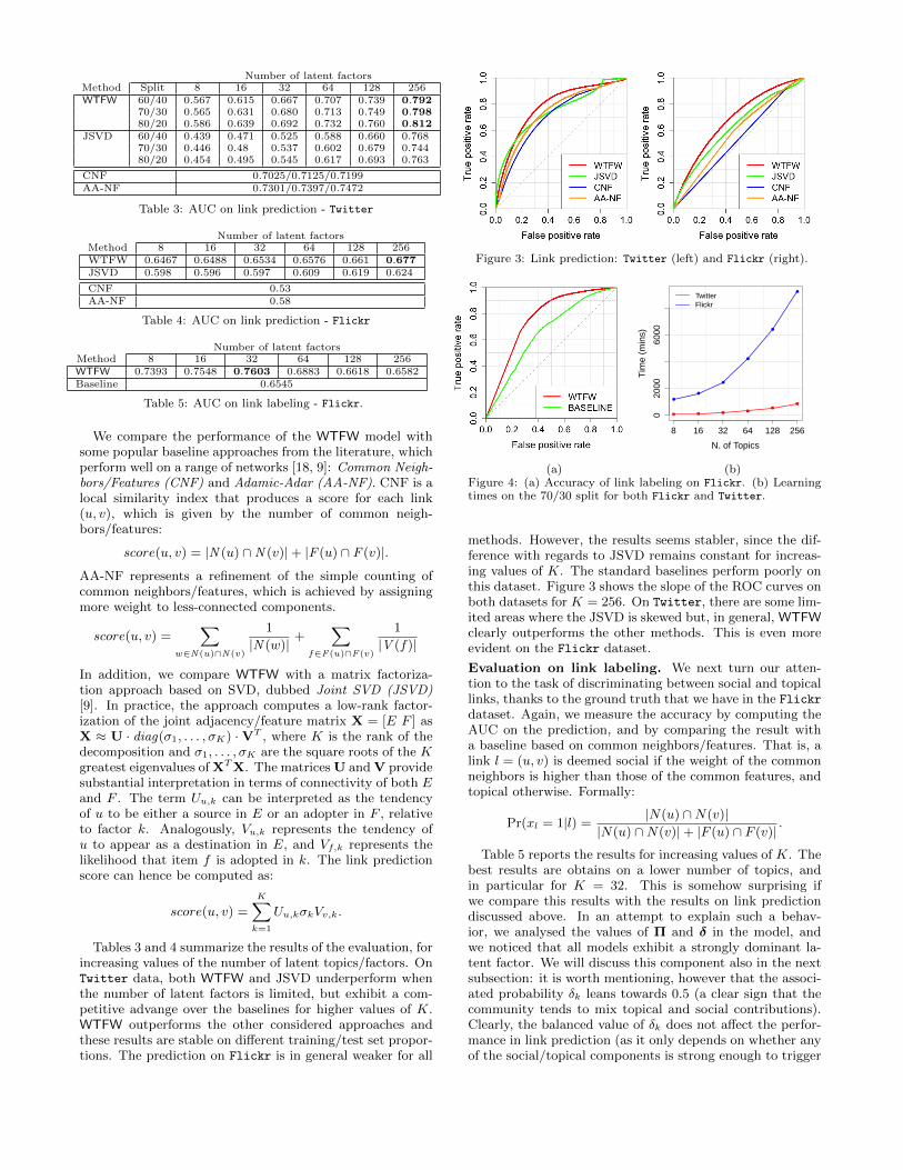
Number of latent factorsMethod Split 8 16 32 64 128 256WTFW 60/40 0.567 0.615 0.667 0.707 0.739 0.792
70/30 0.565 0.631 0.680 0.713 0.749 0.79880/20 0.586 0.639 0.692 0.732 0.760 0.812
JSVD 60/40 0.439 0.471 0.525 0.588 0.660 0.76870/30 0.446 0.48 0.537 0.602 0.679 0.74480/20 0.454 0.495 0.545 0.617 0.693 0.763
CNF 0.7025/0.7125/0.7199AA-NF 0.7301/0.7397/0.7472
Table 3: AUC on link prediction - Twitter
Number of latent factorsMethod 8 16 32 64 128 256WTFW 0.6467 0.6488 0.6534 0.6576 0.661 0.677JSVD 0.598 0.596 0.597 0.609 0.619 0.624
CNF 0.53AA-NF 0.58
Table 4: AUC on link prediction - Flickr
Number of latent factorsMethod 8 16 32 64 128 256WTFW 0.7393 0.7548 0.7603 0.6883 0.6618 0.6582Baseline 0.6545
Table 5: AUC on link labeling - Flickr.
We compare the performance of the WTFW model withsome popular baseline approaches from the literature, whichperform well on a range of networks [18, 9]: Common Neigh-bors/Features (CNF) and Adamic-Adar (AA-NF). CNF is alocal similarity index that produces a score for each link(u, v), which is given by the number of common neigh-bors/features:
score(u, v) = |N (u) ∩N (v)|+ |F (u) ∩ F (v)|.
AA-NF represents a refinement of the simple counting ofcommon neighbors/features, which is achieved by assigningmore weight to less-connected components.
score(u, v) =∑
w∈N (u)∩N (v)
1
|N (w)| +∑
f∈F(u)∩F(v)
1
|V (f)|
In addition, we compare WTFW with a matrix factoriza-tion approach based on SVD, dubbed Joint SVD (JSVD)[9]. In practice, the approach computes a low-rank factor-ization of the joint adjacency/feature matrix X = [E F ] asX ≈ U · diag(σ1, . . . , σK) ·VT , where K is the rank of thedecomposition and σ1, . . . , σK are the square roots of the Kgreatest eigenvalues of XTX. The matrices U and V providesubstantial interpretation in terms of connectivity of both Eand F . The term Uu,k can be interpreted as the tendencyof u to be either a source in E or an adopter in F , relativeto factor k. Analogously, Vu,k represents the tendency ofu to appear as a destination in E, and Vf,k represents thelikelihood that item f is adopted in k. The link predictionscore can hence be computed as:
score(u, v) =
K∑k=1
Uu,kσkVv,k.
Tables 3 and 4 summarize the results of the evaluation, forincreasing values of the number of latent topics/factors. OnTwitter data, both WTFW and JSVD underperform whenthe number of latent factors is limited, but exhibit a com-petitive advange over the baselines for higher values of K.WTFW outperforms the other considered approaches andthese results are stable on different training/test set propor-tions. The prediction on Flickr is in general weaker for all
Figure 3: Link prediction: Twitter (left) and Flickr (right).
020
0060
00
N. of Topics
Tim
e (m
ins)
●
●
●
●
●
●
8 16 32 64 128 256
TwitterFlickr
(a) (b)Figure 4: (a) Accuracy of link labeling on Flickr. (b) Learningtimes on the 70/30 split for both Flickr and Twitter.
methods. However, the results seems stabler, since the dif-ference with regards to JSVD remains constant for increas-ing values of K. The standard baselines perform poorly onthis dataset. Figure 3 shows the slope of the ROC curves onboth datasets for K = 256. On Twitter, there are some lim-ited areas where the JSVD is skewed but, in general, WTFWclearly outperforms the other methods. This is even moreevident on the Flickr dataset.
Evaluation on link labeling. We next turn our atten-tion to the task of discriminating between social and topicallinks, thanks to the ground truth that we have in the Flickrdataset. Again, we measure the accuracy by computing theAUC on the prediction, and by comparing the result witha baseline based on common neighbors/features. That is, alink l = (u, v) is deemed social if the weight of the commonneighbors is higher than those of the common features, andtopical otherwise. Formally:
Pr(xl = 1|l) =|N(u) ∩N(v)|
|N(u) ∩N(v)|+ |F (u) ∩ F (v)| .
Table 5 reports the results for increasing values of K. Thebest results are obtains on a lower number of topics, andin particular for K = 32. This is somehow surprising ifwe compare this results with the results on link predictiondiscussed above. In an attempt to explain such a behav-ior, we analysed the values of Π and δ in the model, andwe noticed that all models exhibit a strongly dominant la-tent factor. We will discuss this component also in the nextsubsection: it is worth mentioning, however that the associ-ated probability δk leans towards 0.5 (a clear sign that thecommunity tends to mix topical and social contributions).Clearly, the balanced value of δk does not affect the perfor-mance in link prediction (as it only depends on whether anyof the social/topical components is strong enough to trigger
1000 2000 3000 4000
Iteration
LogL
iklih
ood/
1,00
0,00
0
−47
.9−
47.7
−47
.5
1000 2000 3000 4000−
984.
0−
983.
8
TwitterFlickr
500 1500 2500 3500
IterationA
UC
0.81
000.
8110
0.81
20
500 1500 2500 3500
0.67
620.
6766
0.67
70
TwitterFlickr
Figure 5: log likelihood and accuracy along the iterations.
1000 2000 3000 4000
0.0
0.1
0.2
0.3
0.4
0.5
Iteration
Per
cent
age
of c
hang
e
XYZe
Zf
500 1500 2500
0.0
0.1
0.2
0.3
0.4
0.5
Flickr
Iteration
Per
cent
age
of c
hang
e
XYZe
Zf
Figure 6: Changes in the matrices Ze, Zf , X and Y.
the link), but it can negatively affect the label prediction.The degradation of the performance for higher values of Kcan find a justification in the split of this giant component:apparently, the splitting seems to produce a reallocation ofthe links in the other communities, thus causing the overfit-ting. Besides this anomalous behavior, WTFW outperformsthe baseline prediction for each considered value of K, asshown in Fig. 4(a).
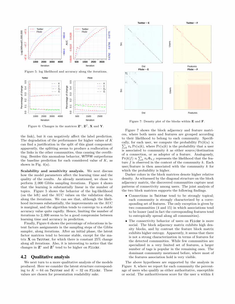
Scalability and sensitivity analysis. We next discusshow the model parameters affect the learning time and thequality of the results. As already mentioned, we chose toperform 2, 000 Gibbs sampling iterations. Figure 4 showsthat the learning is substantially linear in the number oftopics. Figure 5 shows the behavior of the log-likelihood(on the left) and the AUC values on the validation data,along the iterations. We can see that, although the likeli-hood increases substantially, the improvements on the AUCis marginal, and the algorithm tends to converge to a stableaccuracy value quite rapidly. Hence, limiting the number ofiterations to 2, 000 seems to be a good compromise betweenlearning time and accuracy in prediction.
Finally, Figure 6 shows the percentage of relocations in la-tent factors assignments in the sampling steps of the Gibbssampler, along iterations. After an initial phase, the latentfactor matrices tend to become stable, except for the ma-trix X on Twitter, for which there is constant 25% changealong all iterations. Also, it is interesting to notice that thechanges in Ze and Zf tend to be higher on Flickr.
4.2 Qualitative analysisWe next turn to a more qualitative analysis of the models
produced. Here we consider the latent structure correspond-ing to K = 64 on Twitter and K = 32 on Flickr. Thesevalues are chosen for presentation readability sake.
Twitter − E
Dst
Src
Twitter − F
Use
rs
FeaturesFlickr − E
Dst
Src
Flickr − F
Use
rs
Features
Figure 7: Density plot of the blocks within E and F.
Figure 7 shows the block adjacency and feature matri-ces, where both users and features are grouped accordingto their likelihood to belong to each community. Specifi-cally, for each user, we compute the probability Pr(k|u) ∝∑
k πk Pr(u|k), where Pr(u|k) is the probability that a useris associated to community k as either source/destinationof a connection, or as adopter of a feature. Analogously,Pr(k|f) ∝
∑k πkΦk,f represents the likelihood that the fea-
ture f is observed in the context of the community k. Eachuser/feature is then associated with the community k forwhich the probability is higher.
Darker colors in the block matrices denote higher relativedensity. As witnessed by the diagonal structure on the blockadjacency matrix, the discovered communities capture neatpatterns of connectivity among users. The joint analysis ofthe two block matrices supports the following findings.
• Connections in Twitter tend to be strongly topical;each community is strongly characterized by a corre-sponding set of features. The only exception is given bytwo communities (4 and 15) in which associations tendto be looser (and in fact the corresponding features tendto entropically spread along all communities).
• The connectivity behavior of users on Flickr is moresocial. The block adjacency matrix exhibits high den-sity blocks, and by contrast the feature block matrixexhibits higher entropy. Apparently, it seems that thereis not a strong characterization in terms of features forthe detected communities. While few communities arespecialized in a very limited set of features, a largernumber of tags is popular in the remaining ones. Thedominant community mentioned before, where most ofthe features association hold is very visible.
The above hypotheses are supported by the analysis inFigure 8, where we report for each community the percent-age of users who qualify as either authoritative, susceptibleor social. The authoritiveness score for the user u within k

1 3 5 7 9 11 13 15 17 19 21 23 25 27 29 31 33 35 37 39 41 43 45 47 49 51 53 55 57 59 61 63
Community
Per
cent
age
0.0
0.2
0.4
0.6
0.8
1.0
authorities susceptibles social
1 2 3 4 5 6 7 8 9 10 11 12 13 14 15 16 17 18 19 20 21 22 23 24 25 26 27 28 29 30 31 32
Flickr
Community
Per
cent
age
0.0
0.2
0.4
0.6
0.8
1.0
authorities susceptibles social
Figure 8: Proportion of authoritative, susceptible and social users in both Twitter and Flickr.
1 3 5 7 9 11 13 15 17 19 21 23 25 27 29 31 33 35 37 39 41 43 45 47 49 51 53 55 57 59 61 63
Community
Pro
b. S
ocia
l0.
00.
20.
40.
60.
81.
0
1 2 3 4 5 6 7 8 9 10 11 12 13 14 15 16 17 18 19 20 21 22 23 24 25 26 27 28 29 30 31 32
Flickr
Community
Pro
b. S
ocia
l 0.
00.
20.
40.
60.
81.
0
Figure 9: Distribution of δk for each community.
is computed as:
Pr(Auth|u, k) =(1− δk)Ak,u
δkθk,u + (1− δk)(Ak,u + Sk,u).
Scores for measuring the degree of susceptibility and so-ciality can be computed likewise. Again, Twitter tendsto exhibit a predominant amount of authorities/followers,whereas the great majority of the communities in Flickr
tend to include social users. Finally, Figure 9 shows theestimated values of δk within the communities. As alreadyobserved before, Flickr tends to be more clearly social thanTwitter. Moreover, the distinction between social and topi-cal latent factors is very clear in Flickr with almost all com-munities having probability of being “social” either above0.9, or below 0.2. This discriminating attitude is even moreevident when we increase the number of latent topics.
Finally, a further assessment of the correct identificationof social and topical latent factors can be performed by mea-suring, for a given feature f , the probability of observing itin a social/topical context, computed as follows:
Pr(Social |f) ∝∑k
πkδkΦk,f
Pr(Topical |f) ∝∑k
πk(1− δk)Φk,f .
In Table 6 we validate the accuracy of the feature-labelingtask on two small sets of tags. The first set contains key-words notably associated with social events, such as family,and wedding. The second set contains keywords specific tophotographic techniques, e.g. hdr and polaroid, which arelikely to generate topical interest in the users. The resultsconfirm the capability of the model to discriminate betweensocial and topical features.
Finally, Table 7 summarizes the top keywords detected byour approach on both datasets in some representative com-munities/topics: highly social communities (large δ) havecharacteristic features (e.g., family, christmas on Flickr,and followback on Twitter) which are clearly social.
5. CONCLUSIONS AND FUTURE WORKThis paper introduces WTFW, a novel stochastic gener-
ative model that jointly factorizes both social connectionsand feature associations. The model provides accurate linkprediction and contextualized socio/topical explanations tosupport the predictions. Our approach is based on latentfactors which can be interpreted as communities of peoplesharing a similar behavior, and on the explicit modeling of
Feature Prob. Social Feature Prob. Socialbirthday 0.69 hdr 0.40family 0.67 vintage 0.29
wedding 0.69 collage 0.24party 0.67 nude 0.08puppy 0.69 polaroid 0.28
Table 6: Social/Topical connotations of selected tags on Flickr.
Flickr
Topic 1δ = 0.98
Topic 5δ = 0.98
Topic 18δ = 0.17
Topic 22δ = 0.14
Christmas,esther,
passenger,Birthday,
eros, party,stories, apple,
curling,homemade
family, mom,dog, driving,vitus, bakery,
woods,birthday,friends,
halloween,shirt,
brothers,baby
handmade,warehouse,vintage,knitting,
craft, green,pansies, doll,
sewing
bird, art,design,
illustration,drawing, fo-toincatenate,sketch, street,painting, ink,
graffiti
Topic 3δ = 0.74
Topic 9δ = 0.27
Topic 64δ = 0.16
Topic 47δ = 0.33
TeamFollow-Back TFB
FollowNGainfb InstantFol-
lowBacknowplayinglastfm Tea-
mAutoFollowFollow4Follow
500aDayanime 4sqDay
AutodeskBIM
AutoCADRevit AU2012Civil3D AECadsk sf2012
SWTOR revitCAD au2011cloud 3dsMax
AU2011C3D2013
ISS spacescience
DiscoveryMars nasa
spottheshut-tle ESA
astronomyEnterprise
Soyuz
Game-ofThrones
FakeWesterosGoT ooc
SXSWesterosTheGhostofHar-
renhalGardenof-
Bones asoiafGRRM GOT
Table 7: Most representative features of selected communities.
the underlying latent nature behind each observed connec-tion. The result is a decoupling of social and topical con-nections to reflect the idea that social communities shouldhave high density and reciprocal connections, whereas top-ical communities should exhibit clear directionality and alow entropy over user attributes.
Our work can be extended in several directions. First, wedeliberately omitted to quantify the quality of the commu-nities that the model produces. Some initial results basedon modularity look promising (we measured 0.55 and 0.37on Twitter and Flickr, respectively). Also, the qualitativeanalysis in Section 4 clearly denotes the capability of themodel to group users according to both connectivity andcommon features. However, we plan to devote to futurework a more detailed treatment, as well a thorough compar-ison with other approaches in the literature.
Second, the approach explored in this paper is rooted onmixture membership topic modeling. However, other alter-natives are possible, which can be based on probabilisticmatrix factorization. We plan to explore and compare thesedifferent strategies in a future work.

Table 8: Equations for the Gibbs Sampling.
Pr(zl = k|xl = 1,Rest) ∝ (ck + dk + ξk − 1) ·csk + δ0 − 1
ck + δ0 + δ1 − 1·
(cs,sk,ul
+ cs,dk,ul+ αul − 1
)·(cs,sk,vl
+ cs,dk,vl+ αvl − 1
)(2csk +
∑u αu − 1
) (2csk +
∑u αu
)Pr(zl = k|xl = 0,Rest) ∝ (ck + dk + ξk − 1) ·
ctk + δ1 − 1
ck + δ0 + δ1 − 1·ct,sk,ul
+ dsk,ul+ ηul − 1
ctk + dsk +∑
u ηu − 1·ct,dk,vl
+ dak,vl+ βvl − 1
ctk + dak +∑
u βu − 1
Pr(xl = 1|Rest) ∝
(cs,sk,ul
+ cs,dk,ul+ αu − 1
)·(cs,sk,vl
+ cs,dk,vl+ αv − 1
)(2csk +
∑u αu − 1
) (2csk + 1 +
∑u αu − 1
) ·csk + δ0 − 1
csk + ctk + δ0 + δ1 − 1
Pr(xl = 0|Rest) ∝ct,sk,ul
+ dsk,ul+ ηul − 1
ctk + dsk +∑
u ηu − 1·ct,dk,vl
+ dak,vl+ βvl − 1
ctk + dak +∑
u βu − 1·
ctk + δ1 − 1
csk + ctk + δ0 + δ1 − 1
Pr(za = k|ya = 1,Rest) ∝ (ck + dk + ξk − 1) ·dak + τ0 − 1
dak + dsk + τ0 + τ1 − 1·ct,dk,ua
+ dak,ua + βua − 1
ctk + dak +∑
u βu − 1·dk,fd + γfa − 1
dk +∑
f γf − 1
Pr(za = k|ya = 0,Rest) ∝ (ck + dk + ξk − 1) ·dsk + τ1 − 1
dak + dsk + τ0 + τ1 − 1·ct,sk,ua
+ dsk,ua + ηu − 1
ctk + dsk +∑
u ηu − 1·dk,fa + γfa − 1
dk +∑
f γf − 1
Pr(ya = 1|Rest) ∝ct,dk,ua
+ cak,ua + βua − 1
ctk + dak +∑
u βu − 1·
dsk + τ1 − 1
dak + dsk + τ0 + τ1 − 1
Pr(ya = 0|Rest) ∝ct,sk,ua
+ dsk,ua + ηua − 1
ctk + dsk +∑
u ηu − 1·
dak + τ0 − 1
dak + dsk + τ0 + τ1 − 1
(13)
(14)
(15)
(16)
(17)
(18)
(19)
(20)
Acknowledgments. This work was partially supported byMULTISENSOR project, funded by the European Commis-sion, under the contract number FP7-610411.
6. REFERENCES[1] L. Backstrom and J. Leskovec. Supervised random walks:
Predicting and recommending links in social networks. InWSDM, 2011.
[2] N. Barbieri, F. Bonchi, and G. Manco. Cascade-basedcommunity detection. In WSDM, 2013.
[3] C. Bishop. Pattern Recognition and Machine Learning.Springer-Verlag New York, Inc., Secaucus, NJ, USA, 2006.
[4] D. Blei, A. Ng, and M. Jordan. Latent dirichlet allocation. J.Mach. Learn. Res., 3:993–1022, 2003.
[5] F. Bonchi, C. Castillo, A. Gionis, and A. Jaimes. Socialnetwork analysis and mining for business applications. ACMTIST, 2(3):22, 2011.
[6] E. Erosheva, S. Fienberg, and J. Lafferty. Mixed-membershipmodels of scientific publications. PNAS, 101:5220–5227, 2004.
[7] S. Gershman and D. Blei. A tutorial on bayesian nonparametricmodels. Journal of Mathematical Psychology, 56:1–12, 2012.
[8] L. Getoor and C. P. Diehl. Link mining: a survey. SIGKDDExplorations, 7(2):3–12, 2005.
[9] N. Z. Gong, A. Talwalkar, L. W. Mackey, L. Huang, E. C. R.Shin, E. Stefanov, E. Shi, and D. Song. Joint link predictionand attribute inference using a social-attribute network. ACMTIST, 5(2), 2014.
[10] P. A. Grabowicz, L. M. Aiello, V. M. Eguiluz, and A. Jaimes.Distinguishing topical and social groups based on commonidentity and bond theory. In WSDM, 2013.
[11] P. Gupta, A. Goel, J. Lin, A. Sharma, D. Wang, and R. Zadeh.Wtf: the who to follow service at twitter. In WWW, 2013.
[12] M. A. Hasan and M. J. Zaki. A survey of link prediction insocial networks. In Social Network Data Analytics, 2011.
[13] G. Heinrich. Parameter Estimation for Text Analysis.Technical report, University of Leipzig, 2008.
[14] J. L. Herlocker, J. A. Konstan, and J. Riedl. Explainingcollaborative filtering recommendations. In CSCW, 2000.
[15] M. Jamali, T. Huang, and M. Ester. A generalized stochasticblock model for recommendation in social rating networks. InRecSys, 2011.
[16] J. Leskovec and C. Faloutsos. Sampling from large graphs. InKDD, 2006.
[17] D. Liben-Nowell and J. M. Kleinberg. The link predictionproblem for social networks. In CIKM, 2003.
[18] L. Lu and T. Zhou. Link prediction in complex networks: Asurvey. Physica A, 390(6):1150 – 1170, 2011.
[19] K. T. Miller, T. L. Griffiths, and M. I. Jordan. Nonparametriclatent feature models for link prediction. In NIPS, 2009.
[20] T. Minka. Estimating a Dirichlet distribution. Web, 2000.
[21] F. Moser, R. Colak, A. Rafiey, and M. Ester. Mining cohesivepatterns from graphs with feature vectors. In SDM, 2009.
[22] R. M. Nallapati, A. Ahmed, E. P. Xing, and W. W. Cohen.Joint latent topic models for text and citations. In KDD, 2008.
[23] S. Pool, F. Bonchi, and M. van Leeuwen. Description-DrivenCommunity Detection. ACM TIST 5(2): 28, 2014.
[24] D. A. Prentice, D. T. Miller, and J. R. Lightdale. Asymmetriesin Attachments to Groups and to their Members:Distinguishing between Common-Identity and Common-BondGroups. Personality and Social Psychology Bulletin,20(5):484–493, 1994.
[25] P. Pu and L. Chen. Trust building with explanation interfaces.In IUI, 2006.
[26] Y. Ren, R. Kraut, and S. Kiesler. Applying Common Identityand Bond Theory to Design of Online Communities.Organization Studies, 28(3):377–408, 2007.
[27] M. Sachan, D. Contractor, T. A. Faruquie, and L. V.Subramaniam. Using content and interactions for discoveringcommunities in social networks. In WWW, 2012.
[28] V. Sindhwani, S. Bucak, J. Hu, and A. Mojsilovic. One-classmatrix completion with low-density factorizations. In ICDM,2010.
[29] B. Taskar, M. F. Wong, P. Abbeel, and D. Koller. Linkprediction in relational data. In NIPS, 2003.
[30] N. Tintarev and J. Masthoff. Effective explanations ofrecommendations: user-centered design. In RecSys, 2007.
[31] X. Wang, L. Tang, H. Gao, and H. Liu. Discoveringoverlapping groups in social media. In ICDM, 2010.
[32] Z. Xu, Y. Ke, Y. Wang, H. Cheng, and J. Cheng, AModel-based Approach to Attributed Graph Clustering. InSIGMOD, 2012.
[33] Z. Yin, M. Gupta, T. Weninger, and J. Han. Linkrec: a unifiedframework for link recommendation with user attributes andgraph structure. In WWW, 2010.
[34] K. Yu, W. Chu, S. Yu, V. Tresp, and Z. Xu. Stochasticrelational models for discriminative link prediction. In NIPS,2006.
[35] Y. Zhou, H. Cheng, and J. X. Yu. Graph clustering based onstructural/attribute similarities. PVLDB, 2(1):718–729, 2009.