1

Who Provides the Capital for Chinese Growth: The Public or the Private Sector?

Xiaodong Chen1,a, Patrick Minforda,b, Kun Tianc and Peng Zhoua

a Cardiff University, Cardiff, CF10 3EU, UK b CEPR, London, UK c Xiangtan University, China

Abstract

We focus on the role of the government in the provision of investment in China, through the

medium of a DSGE model of the economy in which the form of the production function re-

flects this governmental role. Using indirect inference, we estimate and test for the elasticity

of substitution between government and nongovernment capital in both CES and Cobb-

Douglas technologies. The results underscore the strong substitution relationship between

government and nongovernment capital from 1949, supporting CES rather than the Cobb-

Douglas technology. They also show that the orientation of public investment changed after

the start of the ‘Socialist Market Economy’ in 1992: government capital became more com-plementary to nongovernment capital as it focused more on infrastructure and withdrew from

industrial production, intervening only in times of crisis, for stabilisation purposes, indirectly

via the state banks.

Key Words

China, Government Investment, Indirect Inference, Economic Growth

JEL Classification

E22, E62, O47

1 The corresponding author’s email: chenxd514@hotmail.com.

2

Who Provides the Capital for Chinese Growth: The Public or the Private Sector?

1 Introduction

Public infrastructure is one of the major determinants of economic growth, especially in de-

veloping economies. Public infrastructure can be a bottleneck for sustainable growth and

poverty reduction. The pioneering work of Barro (1990) which incorporates the flow of pub-

lic services into private production is the first endogenous growth model in which long-run

economic growth is driven by fiscal policy. Futagami, Morita and Shibata (1993), Turnovsky

(1997) and Fisher, and Turnovsky (1998) then introduced a stock of public capital as an input

in the production along the lines of the early work of Arrow and Kurz (1970). Other studies

by Baxter and King (1993), Glomm and Ravikumar (1994) and Cassou and Lasing (1998)

also suggest that the accumulated stock of public capital rather than the flow of government

expenditure is more relevant to the production process.

The limit of the early endogenous growth models with fiscal policy in the literature is that

they use a Cobb-Douglas technology to specify the relationship between private and public

capital in production and then restrict the factor substitutability between them to be unity.

More recently, Chatterjee and Ghosh (2011) and Bucci and Del Bo (2012) allow for a flexible

degree of complementarity/substitutability between them by a more general Constant Elas-

ticity of Substitution (CES) aggregate technology. The lack of public capital stock data for a

large number of countries has forced most relevant studies to focus on theoretical analysis

only. Few empirical studies have investigated the effects of public capital on growth, not to

mention the relationship between public and private capital2. The main goal of this paper is to

investigate production technology using Chinese data and to analyse how government pro-

ductive expenditure affects China’s economic growth3. However, many producers in China

are state owned enterprises (SOEs) and township collective enterprises. Hence, for purposes

of accuracy, we use ‘nongovernment capital’ and ‘government capital’, rather than private capital and public capital, to define the two categories of physical capital in production, even

if today nongovernment capital in China is mainly held by private enterprises because of the

economic reform programme.

We find that since 1992 the ‘Socialist Market Economy’ diverted the orientation of public

investment from direct input to industrial production to infrastructure, so that government

capital became more complementary to nongovernment capital.

2 Singh (2012) suggests the long-run crowding-in effects of public capital on private capital in India. 3 Throughout this paper, ‘China’ refers to the mainland China, excluding Taiwan, Hong Kong and Macau.

3

The rest of the paper is organised as follows. The next section introduces some aspects of

China’s economy as the background of our model; section 3 discusses the data; section 4 sets

out the DSGE model to be estimated and tested; sections 5-7 in turn discuss the indirect in-

ference method and the results under two different production functions; section 8 looks at

structural change in 1992. In section 9 we consider the policy implications and section 10

concludes.

2 Stylised Facts of the Chinese Economy: An Overview

China is the fastest growing major economy in the world, with remarkable growth rates, av-

eraging about 8% after 1949 and around 10% over the three decades before 2013. According

to the World Bank (2015), China overtook the United States as the world’s largest economy in 2014, accounting for 17% of the world economy.

Figure 1 demonstrates the six economic troughs after 1949: four of them happened before

1990 and were all because of political disarrays; the other two were caused by external fac-

tors, the 1997 Asian financial crisis and the 2008 global financial and economic crisis. There

were large economic fluctuations before 1978. Since 1978, the economy has achieved rapid

and stable growth.

Figure 1: The Economic Growth Rate in China

Data Source: National Data, National Bureau of Statistics of China.

The Six Economic Troughs since 1949 can be seen in Figure 1 and accounted for as follows:

(i) 1959-1961: ‘Three Years of Natural Disasters’ along with policy failures of the Great Leap Forward; (ii) 1966: the Cultural Revolution; (iii) 1976: the Tangshan earthquake; the

deaths of Zhou Enlai, Zhu De and Mao Zedong; the ousting of the Gang of Four; (iv) 1989:

4

student riots and economic sanctions from Western countries; (v) 1997: the Asian financial

crisis; (vi) 2008: the global financial crisis.

The four stylised facts of the Chinese economy below can be treated as the background for

our model and the comparison between the two subsamples separated by the year of 1992.

2.1 Investment

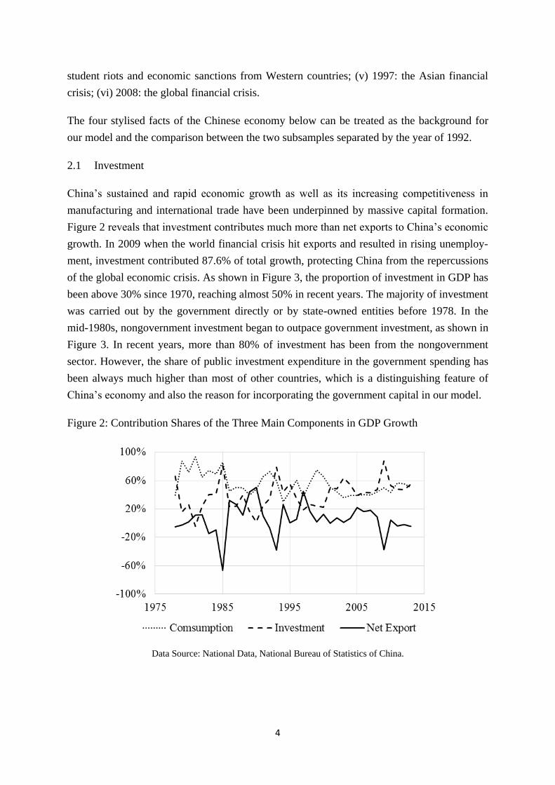
China’s sustained and rapid economic growth as well as its increasing competitiveness in manufacturing and international trade have been underpinned by massive capital formation.

Figure 2 reveals that investment contributes much more than net exports to China’s economic growth. In 2009 when the world financial crisis hit exports and resulted in rising unemploy-

ment, investment contributed 87.6% of total growth, protecting China from the repercussions

of the global economic crisis. As shown in Figure 3, the proportion of investment in GDP has

been above 30% since 1970, reaching almost 50% in recent years. The majority of investment

was carried out by the government directly or by state-owned entities before 1978. In the

mid-1980s, nongovernment investment began to outpace government investment, as shown in

Figure 3. In recent years, more than 80% of investment has been from the nongovernment

sector. However, the share of public investment expenditure in the government spending has

been always much higher than most of other countries, which is a distinguishing feature of

China’s economy and also the reason for incorporating the government capital in our model.

Figure 2: Contribution Shares of the Three Main Components in GDP Growth

Data Source: National Data, National Bureau of Statistics of China.

5

Figure 3: Investment as a Share of GDP

Data Source: The data is calculated on the base of National Data, National Bureau of Statistics of China.

2.2 Human Capital

Production grew substantially between 1949 and the beginning of economic reform in 1978.

Without the political turmoil of that era, China would have had a higher growth rate then. Al-

so, economic growth was accompanied by population growth. As a result, productive capaci-

ty was unable to outrun essential consumption needs by a significant margin, which offset the

efforts of the government to invest more resources in capital goods. The relatively small size

of the capital stock per capita led to low productivity per worker, which in turn perpetuated

the economy’s inability to generate a substantial surplus. In 1979, family planning policy was introduced to alleviate social, economic, and environmental problems in China, averting more

about 300 million births. In the post reform period, productivity rather than population has

accounted for China’s economic growth (see Chow and Li, 2002). Since 1949, human capital

has increased steadily, mainly from the growing population in the first three decades and

from the increasing quality and capability of the workforce in the following three decades. It

is believed that human capital has played an important role in China’s economic miracle (See,

for example, Fleisher and Chen, 1997, Démurger, 2001, and Fleisher, Li and Zhao, 2009).

Hence, our model considers the contribution of human capital which is included in A of the

production function.

2.3 Tax System

Before 1978, public expenditure was mainly financed from the revenues and profits of the

State Owned Enterprises (SOEs). Since 1978, however, the profits claimed by the govern-

ment have been replaced with taxes. In the beginning of this tax reform period, the tax system

0%

10%

20%

30%

40%

50%

1950 1960 1970 1980 1990 2000 2010

Nongovernment Investment/GDP

Government Investment/GDP

Investment/GDP

6

was adjusted for differences in capitalisation and pricing situations among various firms, but

more uniform tax schedules were introduced in the early 1990s. After 1992, value added tax

(proportional to the net value of production) has been the largest revenue resource among all

tax categories. In 2012, tax revenue accounted for 85.8% of government revenue and most

items of tax revenue are proportional rather than progressive. The two progressive tax catego-

ries are individual income tax and land appreciation tax, together accounting for 8.6% of the

total tax revenue in 2012. Since most government tax revenue is proportional to output, we

can simply use a proportional tax in our model.

2.4 The transformation of government functions

Before the early 1990s, central control over planning and the state ownership of the financial

system and certain important industries had enabled the government to mobilise whatever

surplus was available and greatly increase the proportion of GDP devoted to investment. In

1992, Deng Xiaoping made his famous ‘southern tour speech’, following which the ‘socialist market economy’ was legitimised and institutionalised. Since then, private investment4 has

been widely encouraged and it has made up a growing share in total investment. Meanwhile,

the government has changed the structure of public investment by cutting the financial sup-

port to SOEs and inputting more resources in high-quality public infrastructures, which moti-

vates the examination on the possibility of a structural break in 1992 for our model.

In the light of the four features identified above, this paper will examine the elasticity of sub-

stitution between government and nongovernment capital5, investigate the differing orienta-

tion of public investment before and after 1992, and discuss the policy implications.

3 The Data

This paper employs annual data from 1952 to 2012 which is listed in Appendix A. The raw

data are collected from China Statistical Yearbook (2001, 2007, 2008) and National Data,

National Bureau of Statistics of China. The items of raw data are: (i) Gross Domestic Product

(GDP), (ii ) Household Consumption (private consumption or nongovernment consumption),

(iii) Gross Capital Formation (total investment), (iv) Government Budgetary Revenue, (v)

Government Extra-budgetary Revenue, (vi) Government Expenditure by Function (1952-

2006), (vii) Main Items of National Government Expenditure of Central and Local Govern-

4 In this paper, private investment is a part of nongovernment investment since nongovernment sector also in-cludes state owned enterprises and township collective enterprises. 5 The private sector has occupied a larger and larger share in the nongovernment capital since the 1978 reform.

7

ments (2007-2012), (viii) Extra-budgetary Revenue by Item (1952-2010), and (ix) Extra-

budgetary Expenditure by Item6.

The National Bureau of Statistics of China does not directly provide data on government in-

vestment. However, government investment can be approximately estimated by totalling the

corresponding productive expenditure sub-items in the items (vi)-(ix). Thus, nongovernment

investment can be calculated by the gap between total investment and government investment.

Nominal data are transformed into real by dividing by the GDP deflator7.

The tax rate is simply estimated as the share of budgetary plus extra-budgetary revenue in

GDP. We calculate the capital stock values following the conventional ‘Perpetual Inventory

Method’ (PIM)8 expressed as equations (3)-(4) below. The value of the capital stock is esti-

mated by using annual data for capital formation as investment.

4 The Model

Assume that the representative agent maximises lifetime utility:

00

max ,tt t

t

E u c h

, where 1 11 1

,1 1t t

t t

c hu c h

(1)

The model adopts a transformed ‘constant inter-temporal elasticity of substitution’ (CIES) utility function, where c is private consumption (or nongovernment consumption), h is pub-

lic consumption (or government consumption), σ > and σ is the elasticity of marginal utili-

ty with respect to private and public consumption, φ is the weight given to public consump-

tion relative to private consumption. For simplicity, we assume that government capital k ,

tax rate τ and h are exogenous variables, so for the representative, h is determined outside

6 Since 2011, extra-budgetary revenue and expenditure were included in intra-budgetary revenue and expendi-ture. 7 The base year for calculating the GDP deflator is 2000. GDP deflator from 1960 to 2012 is from World Devel-opment Indicators (WDI) & Global Development Finance (GDF), The World Bank (issued in July, 2013); GDP deflator from 1952 to 1959 is calculated from the nominal GDP and indices of GDP (1952-1960). There are no price indices for government investment and nongovernment investment, therefore we use GDP deflator to cal-culate their real values. 8 PIM: The net capital stock at period t, Capital , can be written as a function of its previous value, Capital − , gross investment in period t, Investment , and the depreciation of capital in previous period, Depreciation − : Capital = Capital − + Investment − Depreciation − . Assuming depreciation at a constant rate δ, then we can rewrite the capital stock as: Capital = − Capital − + Investment . The method is called “perpetual” because all assets are forever part of the inventory of capital stocks. The quantity of services provided by an asset declines as it ages, but it never reaches zero. PIM is a popular method of estimating capital stock, for ex-ample, Chow and Li (2002) and Zhang and Zhang (2003) use this method in calculating China’s capital stock, and Kamps (2006) adopts it to provide internationally comparable capital stock estimates for 22 OECD coun-tries. The estimation results in sections 7 and 8 also show the depreciation rates in different periods, which is another contribution to the empirical literature on China.

8

the model. The utility function in the Xie (1997) is a special case of Equation (1) by setting φ = and letting σ approach zero so that the utility follows the logarithm form.

The optimization problem is subject to the budget constraint (2), the laws of motion for the

two capital stocks (3)-(4), and the production function (5) are:

1t t t tc i y (2)

1 1t t ti k k (3)

1 1Gt Gt G Gti k k (4)

1 1 expr r yrt t t t Gt ty f k A k k v

(5)

where A is a deterministic trend which tracks the long-run growth of human capital, includ-

ing both quantity and quality of the labour force9, vy is the logarithm of the productivity

shock, k is nongovernment capital and k is government capital, i is nongovernment in-

vestment and i is government investment, and are the rates of depreciation in non-

government and government sectors.

The homogenous Constant Elasticity of Substitution (CES) production function was intro-

duced by Arrow, Chenery, Minhas and Solow (1961). The elasticity of substitution measures

the percent change in factor proportions due to a one percent change in the marginal rate of

technical substitution. Equation (5) is an extended CES production function which uses a

CES structure to describe the relationship between government and nongovernment capital,

but specifies the relationship between broad physical capital and A in the Cobb-Douglas

form. and − are the share parameters for nongovernment and government capital re-

spectively, − r − is the elasticity of substitution between the two types of capital, θ and − θ are the output elasticities of total capital and A , respectively. If r approaches zero, in

the limit we get the Cobb-Douglas function: 11t exp y

t t t Gt ty f k A k k v .

The equilibrium conditions of the optimisation problem can be derived and stationarised by A following the standard procedure detailed in Appendix B.

9 The production can be write as y = AT P l h −θ[ k + − k ]θr exp(νy), here AT P total factor produc-

tivity, l and h are the quantity and quality of the labour force, hence, A = AT P −θ⁄ l h . Until now, there has been almost no comprehensive method that directly measures the quality of the labour force in China. Moreover, there is no official data on total factor productivity. Nevertheless, we can evaluate A from Equation (5) since we already have the data of output and the two different physical capital stocks.

9

5 Methodology

A DSGE model as such is usually taken to the data using either classical inference (e.g. max-

imum likelihood used by Ireland, 2004; GMM used by Christiano and Eichenbaum, 1992) or

Bayesian inference (e.g. Smets and Wouters, 2003, 2007). With the development of computer

power, there is a trend in macroeconomic literature to use simulation-based inference, such as

indirect inference (Le et al, 2011) which can be used for testing and estimating a DSGE mod-

els. One advantage of indirect inference test is that it provides an absolute verification (or fal-

sification) of the model against the data, while the classical and Bayesian tests (using likeli-

hood ratio and posterior odds) are relative tests between models. A more comprehensive

comparison between these inferences in the scenario of Chinese economy is done in Dai,

Minford and Zhou (2015).

Another advantage of indirect inference is its use of auxiliary model to summarise the data

features. It provides a flexible choice of which aspects you want the model to match. All

models are wrong, but some are useful. It is unlikely for any reasonably complicated model

to match everything. Our model, for example, has a focus on the contribution of capital to

economic growth, so we would like to place higher weights on the capital related dynamics.

VAR is a commonly chosen auxiliary model to summarise the dynamic and volatility features

of the data.

The process of indirect inference testing is to bootstrap the structural residuals and generate a

large number of sample replications, based on which a distribution of the VAR parameters is

obtained; finally to test whether the VAR parameters from actual data lie within this distribu-

tion at some level of confidence. Estimation using indirect inference involves choosing a set

of parameters for the structural model, so that, when this model is simulated, it generates es-

timates of the auxiliary model as close as possible to the estimates of the auxiliary model us-

ing actual data. In other words, indirect estimation chooses the structural parameters that can

minimise the distance between the two sets of estimated parameters. Smith (1993) was the

first to propose this method for estimating nonlinear macro models—see also Gourieroux,

Monfort and Renault (1993) and Canova (2005). The Indirect Inference testing and estima-

tion procedure used here is set out by Dai, Minford and Zhou (2015) in an earlier application

to China and more generally by Le et al (2016) who explain its considerable power in small

samples and the literature in which it was developed.

5.1 The Indirect Inference Test Procedure

The null hypothesis H is that the model is true in the sense that the data behavior as summa-

rized by the auxiliary model, usually a VAR, is close to the simulated data behavior based on

the model. In practice, the test is carried out in the following steps.

10

Step 1: Calculate the Innovations

To recover the innovations (eτ, eK , ey) from the stationarised equation system (Appendix B)

which is derived from the model in Section 4, the parameters need to be calibrated. In par-

ticular, the deterministic growth rate is estimated on the basis of the average growth rates of

GDP and private consumption. For the value of A 95 , set the shocks in the stationarised

equation system as zero, substitute the definition A = A 95 − 95 into the production

function, then obtain the value of ‘A 95 ’ in each year, and obtain A 95 so that the right and

left hand sides are equal at their means. τ and k (the steady states of τ and k ) in the

shock processes are estimated based on the mean values of τ and k . Finally, ρy, ρτ, ρK are

estimated by AR(1) models.

Step 2: Simulate Data

Solve the equation system numerically using Dynare, and then obtain N sets of simulated data

based on N bootstraps of the innovations.

Step 3: Estimate the Auxiliary Model

Use a VAR(1) as the auxiliary model, then estimate it with both actual data and the N sam-

ples of the simulated data. a is obtained from the actual data and includes the VAR parame-

ters and the volatilities of the three variables in the VAR model; (i = , , … N) is obtained

from one sample of simulated data; is the average of N sets of . The auxiliary VAR(1)

model is:

111 21 31

12 22 32 1

13 23 33 1

ˆ ˆ ˆ ˆˆ ˆ ˆ ˆ

ˆ ˆ ˆ ˆ

yt ss t ss t

kt ss t ss t

ct ss t ss t

y y y y

k k k k

c c c c

(6)

where y , k , c are the steady state values of the three endogenous variables: output, non-

government capital and nongovernment consumption in the model.

Step 4: Compute Wald Statistics

1x x xW , where cov i ; x a or 1, ,i N (7)

Compare Wa (the Wald statistics from the actual data) with W95 (the 95th percentile of the

Wald statistics from the simulated data), if Wa is outside the 95% confidence interval, the

model with the selected parameters does not pass the test. In other words, the actual data is

very unlikely to be generated by the model and H should be rejected. Therefore, the model

can be accepted if:

11

951

a

th

WWR

W (8)

5.2 The Indirect Inference Estimation Procedure

As described above, indirect inference can be employed to test whether the model with a giv-

en set of parameters can generate the actual data and the Wald statistic measures the distance

between the observed and the simulated data behaviour. However, if this set of structure pa-

rameters cannot explain the data then another set of parameters may be able to. If no combi-

nation of parameters can be found under which the model passes, then the model should be

rejected. Even if the model has already passed the test, it is still necessary to seek an alterna-

tive set of parameters that could reduce the value of WR. The main idea of indirect inference

estimation is to search for the optimal set of parameters which minimises the value of WR.

6 Indirect Inference Test Results

This section looks at the indirect inference test results of the calibrated model under both

CES production function and Cobb-Douglas as a special case. Based on the assumed parame-

ters, our test results accept the CES production function and reject the more restrictive Cobb-

Douglas specification.

The key aspects of PIM are to set the base year capital stock and to estimate the asset depre-

ciation rates. Table 1 and Table 2 show that different values of initial capital stock and depre-

ciation rate have been used in the literature and the choices are controversial. Any initial val-

ue of capital stock (the capital stock in 1952) with moderate depreciation rates makes the ra-

tio of total capital to GDP around 2 during the period after 1960, which suggests the capital-

GDP ratio is about 2 (See Figure 4), similar to those in other countries. The GDP in 1952 was

about 274 billion, therefore, the indirect inference test sets the initial capital stock as 600 bil-

lion Yuan with the price level in 2000, which is close to Wang and Fan (2000). For the esti-

mations in the next section, the initial capital stock is allowed to range from 500 to 800 bil-

lion Yuan. Since government and nongovernment investment from 1952 to 1954 are rather

close, it is reasonable to assume the initial capital was almost equally divided into govern-

ment and nongovernment sectors. Hence, the initial values of the two types of physical capi-

tal are both set as 300 billion in the test10.

10 The initial value of capital does not have a large effect on the future capital after several years due to a large depreciation rate. Our experiments show that different sets of initial values of nongovernment and government capital only lead to rather small gaps between their corresponding empirical results, especially in the period from 1993 to 2012.

12

Table 1: Literature of Initial Capital Stock in China (in 2000 prices, billion Yuan)

Literature Capital Stock in 1952 Zhang (1991), cited in Zhang and Zhang (2003) 808.1 He (1992), cited in Zhang and Zhang (2003) 186.5 Chow (1993) 707.1 Perkins (1998), cited in Wu (2009) 832.3 Chow and Li (2002) 894.1 Wang and Fan (2000) 646.5 Zhang and Zhang (2003) 323.2

Table 2 provides the literature of depreciation rate in China. The selection of depreciation

rates of both types of physical capital in Equation (3) and Equation (4) follows Zhang (2008)

with 9.6% in the test, and the rates are in an interval from 7% to 12% for estimations.

Table 2: Literature of Depreciation Rate in China (%)

Literature Depreciation Rate World Bank (1997), cited in Wu (2009) 4.0 Perkins (1998), cited in Wu (2009) 5.0 Chow and Li (2002) 5.4 Wu (2004) 7.0 Maddison (2007) 17.0 Zhang (2008) 9.6

The study of Luo and Zhang (2009) shows that the labour income share in GDP drops from

52% in 1987 to 40% in 2006; while Bai and Qian (2010) have it that the labour income share

in the industry sector increased from 34.52% to 42.21% in the period between 1978 and 2004.

The labour income share is much lower in China than in the US and most of other countries,

in other words, the capital income share in China is higher than that in most of other countries.

Since there is government capital in the production function, the elasticity of output with re-

spect to total capital should be higher than the capital income share. The average ratio of

nongovernment capital to government capital is about 5:4 in the period from 1952 to 2012.

Hence, the value of θ in Equation (5) is possibly in the interval from 0.55 to 0.75. The value

in testing can be set as 2/3=0.667. Many studies adopt a 3 percent or a little larger discount

rate according to the real rate of interest on Treasury bonds or other economic figures, there-

fore, the rate of time preference in Equation (1) is fixed as = . for tests with the data in

China, a future-oriented society, and between the lower bound 0.96 and the upper bound 0.99

in estimation.

Table 3 gives the test results with the CES production function, showing that the model pass-

es the test since WR < . Moreover, all VAR parameters and variances from the actual data

13

are within the 95% lower and upper bounds, in other words, based on the assumed parameters,

the model with the CES production function captures the data behaviour well.

Table 3: Test Results of the Model with Different Production Functions

Auxiliary Parameters

CES IN/OUT11 Cobb-Douglas IN/OUT

0.8206 IN 0.8452 IN

0.0573 IN 0.0533 IN

0.1703 IN 0.1856 IN

-0.0978 IN -0.0144 IN

1.0737 IN 1.0554 OUT

-0.1834 IN -0.2703 OUT

0.0102 IN 0.0195 IN

0.0053 IN 0.0037 IN

0.9446 IN 0.9489 IN var y 0.0268 IN 0.0182 IN var k 0.2771 IN 0.1885 OUT var c 0.0095 IN 0.0065 IN Wa 10.3766

IN 1383.2690

OUT WR 0.3367 < 1 46.3973 > 1

The calibrated values of the parameters are: k 95 = , k 95 = , = . , =. , = . ,θ = . , = . , r = , σ = . , = . A 95 , τ , k , ρy, ρτ, ρK are

estimated by the indirect inference method.

The test of the model with Cobb-Douglas production function adopts the same values of k 95 , k 95 , , , , θ, , r, σ as in the test with CES production function above, while the

values of A 95 , τ , k , ρy, ρτ, ρK are re-estimated. Table 3 shows that, with the Cobb-

Douglas production function, the Wald statistic from the test is very high. Hence, we cannot

accept the Cobb-Douglas production function under the assumed parameters.

According to the testing results, the CES production function is much better than the Cobb-

Douglas production function, which is not surprising since the CES production function is a

more general case. The results imply the elasticity of substitution between the two types of

capital / − r is extremely high since the test result becomes better as r gets close to 1.

11 IN means ‘inside the 95% confidence interval’; OUT means ‘outside the 95% confidence interval’.

14

Figure 4 may justify these apparently odd results. The ratio of total capital to GDP is rather

stable, while the ratio of nongovernment capital to GDP doubled in the six decades and the

ratio of government capital had decreased to less than half of the initial ratio, suggesting there

may be a strong substitution relation between the two types of capital.

Figure 4: Ratios of Nongovernment, Government and Total Capital to GDP

Note: The data is estimated by setting k 95 = , k 95 = , = . , = . .

Table 4 shows that the two types of capital are gross substitutes (< r ≤ ). The model

passes the test when r = . but gets closest to the data behaviour when the two types of cap-

ital are perfect substitutes (r = . WE show the details in the following section.

Table 4: Test Results with Different Values of � � �� � 0 0.2 0.4 0.6 0.8 1 Wa 1383.2690 373.5062 114.4094 39.0750 16.4111 10.3766 WR 46.3973 13.0236 3.9217 1.3285 0.5401 0.3367

7 Indirect Inference Estimation Results

Table 5 shows that the set of estimated parameters (i.e. the parameters that get closest to the

data behaviour) under the CES production function captures the reality well with a low Wald

statistic and a low value of WR. The impulse response functions for this model are listed in

Appendix C.

15

Table 5: Estimation Results of the Model with Different Production Functions

Auxiliary Parameters

CES IN/OUT Cobb-Douglas IN/OUT

0.7923 IN 0.5924 OUT

0.0775 IN 0.1278 IN

0.1818 IN 0.3969 IN

-0.0791 IN 0.1180 IN

1.1108 IN 1.0340 OUT

-0.3322 IN -0.4426 OUT

-0.0060 IN -0.0685 OUT

0.0112 IN 0.0299 IN

0.9519 IN 1.0409 IN var y 0.0437 IN 0.0122 OUT var k 0.3445 IN 0.1163 IN var c 0.0036 IN 0.0032 IN Wa 4.8892

IN 50.9957

OUT WR 0.1502 < 1 1.7445 > 1

The estimated parameter values can be found in Table 6. The estimated elasticity of substitu-

tion r is close to 1, implying a strong substitution between government and nongovernment

capital. Most estimated parameters under CES technology are close to the calibrated values,

while the estimated initial government capital in 1952 is much higher than the calibrated one.

However, even if we restrict the initial government capital to the calibrated value, other CES

estimated parameters still yield a small value of WR and the CES model passes the test easily.

In contrast, the model with the Cobb-Douglas production function does not pass the test

(Table 5): the Wald statistic is very large and the value of WR is larger than 1, which means

that no set of estimated parameter under the Cobb-Douglas production function can capture

actual date behaviour well. Hence, the Cobb-Douglas production function is not suitable to

describe the relationship between government and nongovernment capital. The estimated pa-

rameter values can be found in Table 6.

8 Structural Break

As argued in the introduction and Subsection 2.4, we examine the possibility of a structural

break in 1992, the time of Deng Xiaoping’s important south tour speech.

16

The estimated parameter values of the two subsamples are compared with those of the whole

sample in Table 6. The small values of Wald statistics (3.9566) and WR = . < sug-

gest that, based on the data from 1952 to 1992, the model with CES production function can

be accepted. All actual VAR coefficients and volatilities are within the 95% lower and upper

bounds. Again, r is close to 1, which still implies strong substitution between government

capital and nongovernment capital from 1952 to 1992. Similarly, Wald statistics (10.1558)

and WR = . < are small, so that, based on the data from 1993 to 2012, the model

with CES production function can be accepted. All actual VAR coefficients and volatilities in

this period are within the 95% lower and upper bounds.

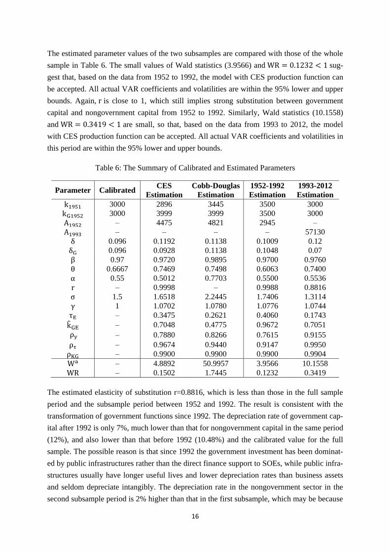
Table 6: The Summary of Calibrated and Estimated Parameters

Parameter Calibrated CES Estimation

Cobb-Douglas Estimation

1952-1992 Estimation

1993-2012 Estimation k 95 3000 2896 3445 3500 3000 k 95 3000 3999 3999 3500 3000 A 95 – 4475 4821 2945 – A 99 – – – – 57130

0.096 0.1192 0.1138 0.1009 0.12 0.096 0.0928 0.1138 0.1048 0.07 0.97 0.9720 0.9895 0.9700 0.9760 θ 0.6667 0.7469 0.7498 0.6063 0.7400 0.55 0.5012 0.7703 0.5500 0.5536 r – 0.9998 – 0.9988 0.8816 σ 1.5 1.6518 2.2445 1.7406 1.3114 1 1.0702 1.0780 1.0776 1.0744 τ – 0.3475 0.2621 0.4060 0.1743 k – 0.7048 0.4775 0.9672 0.7051 ρy – 0.7880 0.8266 0.7615 0.9155 ρτ – 0.9674 0.9440 0.9147 0.9950 ρK – 0.9900 0.9900 0.9900 0.9904 Wa – 4.8892 50.9957 3.9566 10.1558 WR – 0.1502 1.7445 0.1232 0.3419

The estimated elasticity of substitution r=0.8816, which is less than those in the full sample

period and the subsample period between 1952 and 1992. The result is consistent with the

transformation of government functions since 1992. The depreciation rate of government cap-

ital after 1992 is only 7%, much lower than that for nongovernment capital in the same period

(12%), and also lower than that before 1992 (10.48%) and the calibrated value for the full

sample. The possible reason is that since 1992 the government investment has been dominat-

ed by public infrastructures rather than the direct finance support to SOEs, while public infra-

structures usually have longer useful lives and lower depreciation rates than business assets

and seldom depreciate intangibly. The depreciation rate in the nongovernment sector in the

second subsample period is 2% higher than that in the first subsample, which may be because

17

the nongovernment assets, such as machinery and vehicles, have experienced higher intangi-

ble depreciation due to the dramatic technology advances since the begging of ‘socialist mar-ket economy’ in 1992.

The lower value of elasticity of substitution between government capital and nongovernment

capital after 1992 suggests that the government has become more complementary to the non-

government sector. The estimation result with CES production function ties in with the fact

that China has deepened the reforms of SOEs and fiscal policies since 1992.

9 Discussion and Policy Implications

As illustrated by both test and estimation results, there is a strong substitution relationship

between government and nongovernment capital. The estimation for CES technology is gen-

erally close to the calibration, which enforces reinforce our conclusion. Hence, the Cobb-

Douglas specification cannot be applicable to China’s macroeconomy, especially when the

economy was based on the dominance of the state-owned sector before 1992. Our empirical

findings identify the potential problems in previous studies, such as Barro (1990) and

Turnovsky (1997): they do not address the issue of different degrees of complementari-

ty/substitutability between the two types of capital.

The substitution relationship between government and nongovernment sectors was in line

with the reality in China before 1992. Influenced by the Soviet Union, the Chinese govern-

ment nationalised virtually most private industrial enterprises during the 1950s. A large pro-

portion of government productive expenditure was poured into SOEs. Under a centrally

planned economy, the government ‘invaded’ the private sector, making the difference be-

tween government and nongovernment investment ambiguous. In other words, sometimes the

government did what the nongovernment sector should do. After 1978, the government initi-

ated intensive reforms and private investment was encouraged. In 1990s, some SOEs were

privatised. Nongovernment capital, especially private capital, then ‘fought back’ into the field

once occupied by the nongovernment capital.

In the 1980s and 1990s, the Chinese government intentionally reduced its share of GDP in

order to allow rural and urban households and firms to have more resources and better incen-

tives. Furthermore, the SOEs tended to be more market orientated and could not receive pub-

lic investment freely. Meanwhile, public productive investment flowed to infrastructure con-

struction rather than SOEs. The government became a service supplier. Government and

nongovernment capital stocks became more complementary, which is verified by the estimat-

ed r being reduced from close to 1 in the period between 1952 and 1992 to 0.8816 after 1992.

18

The merits and drawbacks of large-scale public investment were thoroughly exhibited in the

Maoist era. In that period, consumption, especially in rural areas, was contained by taxes and

compulsory delivery quotas, which were imposed in order to finance public investment and

feed the urban population at low prices. Absolute egalitarianism totally destroyed market

forces. Enthusiasm for work was mainly from discipline and political beliefs rather than eco-

nomic benefits. Nevertheless, economic performance was greatly improved, as argued by

Maddison (2007). Real GDP had expanded more than fivefold from 1949 to 1976; human

capital and labour productivity were also enhanced due to better education and doubled aver-

age life span; the economic structure was transformed with industry’s share of GDP increas-

ing from one tenth to almost one half. China achieved this despite the self-inflicted wounds

that hampered economic growth during the Great Leap Forward (1958-1960) and the Cultural

Revolution (1966-1976), China’s political and economic isolation, and its hostile diplomatic

relations with both the United States and the Soviet Unions. Obviously, without the political

instability and the economic sanctions imposed by some Western countries, China would

have enjoyed a better economic performance from its development effort and large-scale pub-

lic investment. We cannot jump rashly to the conclusion that the macroeconomy before the

1978 reform was a complete failure. However, it is safe to draw the conclusion that Deng

Xiaoping’s path of opening up and economic reform was superior to the development strate-

gies before the reform, as evidenced by higher and more stable economic growth after 1978.

Committing to continuing Deng Xiaoping’s path, China has adopted fiscal policies to deal

with the trade-off in the public investment, as simply summarised in three aspects below.

Firstly, the government is decentralising the economy, partially privatising the SOEs and

transforming most of them into joint-stock companies. The state retains ownership of some

large SOEs but has little direct control over their operations. Moreover, the government does

not pour public investment into SOEs freely any longer, which lessens the financial burden of

the government, making it possible to reduce the tax rate so that households and firms have

more resources and better incentives.

Secondly, the government has changed the structure of public investment. By stopping the

free injection of funds into SOEs and cutting the financial support to them, the government

has more resources to invest in high-quality and large-quantity infrastructures and improve

the investment environment. The government directly or indirectly (through SOEs) builds

more expressways, international airports, high-speed railways and telecommunication facili-

ties. The government has transformed itself from being a competitor of the private sector to

being a service provider to private investors.

Lastly, the government is using public investment, together with other policies, as a tool for

stabilising the economy when faced with slipping business confidence domestically or exter-

19

nally. Beijing’s response to the 2008 economic crisis was swift: development of polysilicon

supplies and manufacturing technology of clean cars were declared as national priorities with

financial support and tax advantages. Money poured into manufacturers and overseas acquisi-

tion of cheap assets, resources and technology from state-owned companies and banks, local

governments expedited approvals for new plants. The leveraged investment from the gov-

ernment and SOEs offset the reduction of private investment, reduced unemployment, and

finally restored confidence and liquidity, achieving rather high annul growth rates: 9.6%, 9.2%

and 10.4% from 2008 to 2010. In 2009, 7.6% of growth was contributed by investment.

In sum, the Chinese government began post-war by dominating the economy with public in-

vestment, substituting actively for investment in areas that would have been provided for by

the private sector in a non-communist economy. However, after 1978 and particularly after

the reforms of 1992, it increasingly withdrew from these areas and concentrated on the provi-

sion of infrastructure, only reentering them in times of crisis for stabilisation reasons and

even in those times indirectly via the active direction of credit from the state-controlled banks.

10 Conclusion

This paper focuses on the role of the government in the provision of investment in China,

through a DSGE model of the economy in which the form of the production function reflects

this governmental role. Specifically, using the method of indirect inference, we estimate and

test for the elasticity of substitution between government and nongovernment capital in both

CES and Cobb-Douglas technologies. Both test and estimation results underscore the strong

substitution relationship between government and nongovernment capital after the founding

of People’s Republic of China in 1949, and thus the general CES technology rather than the

Cobb-Douglas technology is the suitable structure for modelling the two types of capital in

the production function.

Furthermore, the estimation results corroborate the way in which the orientation of public in-

vestment changed after the start of the ‘Socialist Market Economy’ in 1992. From this point

onwards government capital became more complementary to nongovernment capital as it fo-

cused more on infrastructure and withdrew from industrial production. It only deviated from

this focus in times of crisis, especially the recent world financial crisis, for reasons of macro

stabilisation; even then it did so indirectly via the state banks.

20

References

Arrow, K., Chenery, H., Minhas, B. and Solow, R. 1961. Capital-labor substitution and eco-nomic efficiency. The Review of Economics and Statistics 43(3), pp. 225-250.

Arrow, K. and Kurz, M. 1970. Public Investment, the Rate of Return, and Optimal Fiscal

Policy. Baltimore: The John Hopkins Press.

Bai, C. and Qian, Z. 2010. The factor income distribution in China: 1978–2007. China Eco-

nomic Review 21, pp. 650-670.

Barro, R. 1990. Government spending in a simple model of endogenous growth. Journal of

Political Economy 98, pp. S103-S125.

Baxter, M. and King, R. 1993. Fiscal policy in general equilibrium. The American Economic

Review 83, pp. 315-334.

Bucci, A. and Del Bo, C. 2012.On the Interaction between Public and Private Capital in Eco-nomic Growth. Journal of Economics 106(2), pp. 133–152.

Canova, F. 2005. Methods for Applied Macroeconomic Research. Princeton: Princeton Uni-versity Press.

Cassou, S. P. and Lansing, K. J. 1998. Optimal Fiscal Policy, Public Capital, and the Produc-tivity Slowdown. Journal of Economic Dynamics and Control 22(6), pp. 911-935.

Chatterjee, S. and Ghosh, S. 2011. The dual nature of public goods and congestion: the role of fiscal policy revisited. Canadian Journal of Economics 44(4), pp. 1471-1496.

Chow, G. 1993. Capital formation and economic growth in China. Quarterly Journal of Eco-

nomics 108, pp. 809-842.

Chow, G. and Li, K. 2002. China’s economic growth: 1952–2010. Economic Development

and Cultural Change 51(1), pp. 247-256.

Christiano, L. and Eichenbaum, M. 1992. Current Real-Business-Cycle Theories and Aggre-gate Labor-Market Fluctuations. The American Economic Review 82 (3): 430-450.

Dai, L., Minford, P. and Zhou, P. 2015. A DSGE Model of China, Applied Economics 47(59), pp. 6438-6460.

Démurger, S. 2001. Infrastructure Development and Economic Growth: An Explanation for Regional Disparities in China? Journal of Comparative Economics 19, pp. 95-117.

Fisher, W. and Turnovsky, S. 1998. Public investment, congestion, and private capital accu-mulation. Economic Journal 108, pp. 399-413.

Fleisher, B. and Chen, J. 1997. The Coast-Noncoast Income Gap, Productivity and Regional Economic Policy in China. Journal of Comparative Economics 252, pp. 220-236.

Fleisher, B., Li, H. and Zhao, Mi. 2009. Human Capital, Economic Growth, and Regional Inequality in China. Journal of Development Economics 92(2), pp. 215-231.

21

Futagami, K., Morita, Y. and Shibata, A. 1993. Dynamic analysis of an endogenous growth model with public capital. Scandinavian Journal of Economics 95(4), pp. 607-625.

Glomm, G. and Ravikumar, B. 1994. Public investment in infrastructure in a simple growth model. Journal of Economic Dynamics and Control 18, pp. 1173-1187.

Gourieroux, C. Monfort, A. and Renault, E. 1993. Indirect inference. Journal of Applied

Econometrics 8, pp. S85-S118.

Ireland, P. 2004. A Method for Taking Models to the Data. Journal of Economic Dynamics

and Control 28, pp. 1250-1226.

Kamps, C. 2006. New Estimates of Government Net Capital Stocks for 22 OECD Countries, 1960-2001. IMF Staff Papers 53(1), pp. 120-150.

Le, V., Meenagh, D. Minford, P. and Wickens, M. 2011. How much nominal rigidity is there in the US economy? Testing a new Keynesian DSGE model using indirect inference. Journal

of Economic Dynamics and Control 35(12), pp. 2078-2104.

Le, V., Meenagh, D., Minford, P., Wickens, M. and Xu, Y. 2016. Testing macro models by indirect inference: a survey for users. Open Economies Review 27(1), pp. 1-38.

Luo, C. and Zhang, J. 2009. Explaining the decrease of labour income share by Economics analysis on the basis of panel data of Chinese provinces. Management World (Guanli Shijie) 5, pp. 25-35.

Maddison, A. 2007. Chinese Economic Performance in the Long Run. 2nd ed. Development Centre, OECD.

National Bureau of Statistics of China. 2001, 2007, 2008. China Statistical Yearbook. Beijing: China Statistics Press.

Singh, T. 2012. Does Public Capital Crowd-Out or Crowd-In Private Capital in India? Jour-

nal of Economic Policy Reform 15(2), pp. 109-133.

Smets, F. and Wouters, R. 2003. An Estimated Dynamic Stochastic General Equilibrium Model of the Euro Area. Journal of the European Economic Association 1(5), pp. 1123–1175.

Smets, F. and Wouters, R. 2007. Shocks and Frictions in US Business Cycles: A Bayesian DSGE Approach. The American Economic Review 97(3), pp. 586-606.

Smith, A.1993. Estimating nonlinear time series models using simulated vector autoregres-sions. Journal of Applied Econometrics 8, pp. S63-S84.

Turnovsky, S. 1997. Fiscal policy in a growing economy with public capital. Macroeconomic

Dynamics 1(3), pp. 615-639.

Wang, X. and Fan, G. 2000. The Sustainability of China’s Economic Growth (in Chinese). Beijing: Economic Sciences Press.

World Bank. 2015. Gross domestic product 2014, PPP. [Online] Available at: http://databank.worldbank.org/data/download/GDP_PPP.pdf

22

Wu, Y. 2004. China’s Economic Growth: A Miracle with Chinese Characteristics. London and New York: Routledge Curzon Press Limited.

Wu, Y. 2009. China's Capital Stock Series by Region and Sector. Discussion Paper, Business School, University of Western Australia.

Zhang, J. and Zhang, Y. 2003. Reestimates of China’s capital stock K. Journal of Economic Research (Jingji Yanjiu) 7, pp. 35-43.

Zhang, J. 2008. Estimation of China’s provincial capital stock (1952-2004) with applications. Journal of Chinese Economic and Business Studies 6(2), pp. 177-196.

Xie, D. 1997. On Time inconsistency: a technical issue in Stackelberg differential games. Journal of Economic Theory 76, pp. 412-430.

23

Appendix A: Real Data (1952-2012) 100 million Yuan

GDP Nongovernment Consumption

Nongovernment Investment

Government Investment

Tax Rates

1952 2743.95 1830.64 316.79 304.33 0.28 1953 3265.02 2096.90 433.92 351.82 0.27 1954 3437.42 2200.91 404.76 503.21 0.30 1955 3647.27 2415.21 325.78 561.99 0.29 1956 4155.76 2614.73 384.82 656.55 0.29 1957 4307.32 2769.11 455.51 673.75 0.31 1958 5222.65 2893.04 577.80 1148.43 0.33 1959 5683.32 2729.89 859.56 1595.84 0.41 1960 5614.64 2858.19 371.18 1844.62 0.47 1961 4199.66 2811.36 192.19 753.07 0.34 1962 4004.53 2922.30 54.88 565.67 0.33 1963 4382.73 3000.00 295.91 646.88 0.32 1964 5134.18 3141.24 459.96 776.97 0.32 1965 5927.81 3286.70 678.62 917.58 0.32 1966 6563.60 3587.84 871.37 1130.74 0.34 1967 6189.46 3773.55 589.37 895.98 0.28 1968 5935.58 3708.58 876.18 612.63 0.25 1969 6938.42 4037.59 633.88 1105.83 0.32 1970 8285.03 4438.40 1239.02 1500.59 0.34 1971 8865.18 4610.89 1397.92 1594.41 0.36 1972 9200.22 4874.68 1237.34 1653.06 0.36 1973 9926.67 5226.19 1481.37 1814.87 0.37 1974 10156.17 5340.37 1607.74 1799.98 0.36 1975 11039.78 5629.83 1997.31 1915.39 0.36 1976 10862.36 5861.62 1778.13 1875.37 0.36 1977 11690.03 6016.06 2033.12 1976.00 0.37 1978 13055.95 6300.50 2170.35 2764.83 0.41 1979 14047.65 6955.39 2212.69 2901.07 0.39 1980 15147.02 7768.08 2663.10 2667.46 0.38 1981 15933.42 8559.93 2956.79 2353.31 0.36 1982 17379.53 9477.31 2425.11 3399.90 0.38 1983 19277.89 10446.49 2812.19 3780.12 0.39 1984 22205.95 11528.03 3381.21 4367.10 0.39 1985 25205.59 13104.28 4916.61 4749.32 0.39 1986 27422.42 14150.25 5888.66 4631.49 0.38 1987 30605.63 15548.48 6518.02 4806.85 0.35 1988 34064.36 17817.26 8212.25 4695.81 0.31 1989 35459.77 18390.23 8715.88 4499.27 0.31 1990 36805.64 18633.48 8779.73 4522.71 0.30 1991 40194.69 19801.81 9937.37 4581.92 0.29 1992 45897.51 22161.78 12154.53 5039.98 0.27 1993 52323.29 24303.42 20128.59 3146.54 0.16 1994 59182.05 26822.45 21295.33 3681.46 0.15 1995 65630.71 30626.90 23446.85 4049.75 0.14 1996 72194.53 34441.53 24405.00 4791.57 0.16 1997 78909.90 36891.99 25798.00 4146.04 0.15 1998 85065.79 39537.69 26950.93 4609.44 0.15 1999 91525.87 42784.65 27914.08 5716.76 0.17 2000 99214.55 45854.60 28668.24 6174.56 0.17 2001 107452.40 48442.78 32285.00 6685.51 0.19 2002 117226.20 51686.87 37634.00 6754.70 0.19 2003 128949.74 54732.56 46312.63 6818.48 0.19 2004 141975.26 57915.35 54122.97 7300.00 0.19 2005 158012.11 62336.56 58264.80 8256.75 0.20 2006 178080.54 67980.12 67335.95 9188.36 0.21 2007 203374.38 73705.05 73950.23 10933.67 0.22 2008 222901.15 79260.70 83867.19 14312.45 0.22 2009 243397.69 88236.91 96675.93 20747.47 0.22 2010 268714.23 94203.35 107513.19 22057.09 0.22 2011 293707.51 104889.89 120040.23 21718.07 0.22 2012 316711.44 116195.95 128529.96 25581.27 0.23

24

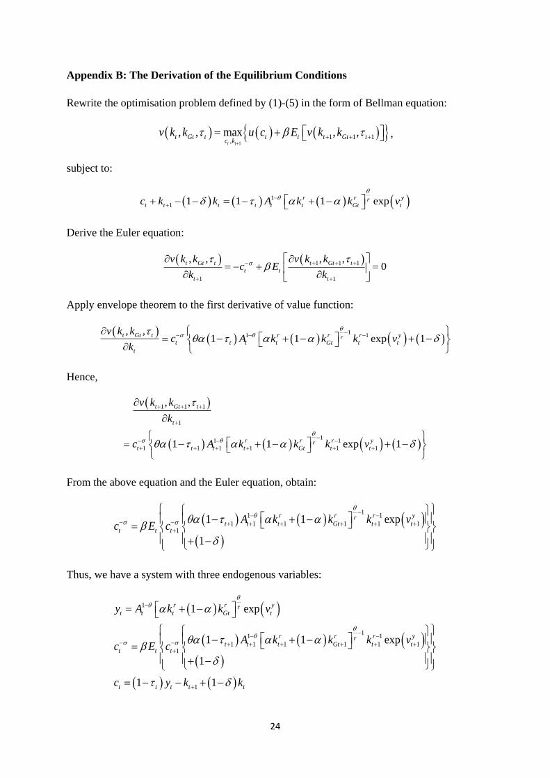
Appendix B: The Derivation of the Equilibrium Conditions

Rewrite the optimisation problem defined by (1)-(5) in the form of Bellman equation:

1

1 1 1,

, , max , ,t t

t Gt t t t t Gt tc k

v k k u c E v k k ,

subject to:

11 1 1 1 expr r yr

t t t t t t Gt tc k k A k k v

Derive the Euler equation:

1 1 1

1 1

, , , ,0t Gt t t Gt t

t tt t

v k k v k kc E

k k

Apply envelope theorem to the first derivative of value function:

11 1, ,1 1 exp 1t Gt t r r r yr

t t t t Gt t tt

v k kc A k k k v

k

Hence,

1 1 1

1

11 11 1 1 1 1 1

, ,

1 1 exp 1

t Gt t

t

r r r yrt t t t Gt t t

v k k

k

c A k k k v

From the above equation and the Euler equation, obtain:

11 11 1 1 1 1 1

1

1 1 exp

1

r r r yrt t t Gt t t

t t t

A k k k vc E c

Thus, we have a system with three endogenous variables:

1

11 11 1 1 1 1 1

1

1

1 exp

1 1 exp

1

1 1

r r yrt t t Gt t

r r r yrt t t Gt t t

t t t

t t t t t

y A k k v

A k k k vc E c

c y k k

25

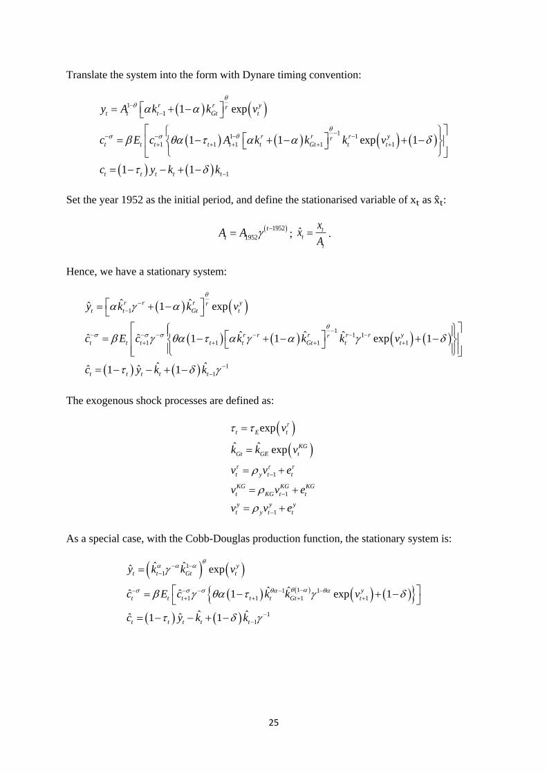
Translate the system into the form with Dynare timing convention:

11

11 11 1 1 1 1

1

1 exp

1 1 exp 1

1 1

r r yrt t t Gt t

r r r yrt t t t t t Gt t t

t t t t t

y A k k v

c E c A k k k v

c y k k

Set the year 1952 as the initial period, and define the stationarised variable of x as x :

19521952

ttA A ; ˆ t

tt

xx

A .

Hence, we have a stationary system:

1

11 1

1 1 1 1

11

ˆ ˆˆ 1 exp

ˆ ˆ ˆˆ ˆ 1 1 exp 1

ˆ ˆˆ ˆ1 1

r r r yrt t Gt t

r r r r r yrt t t t t Gt t t

t t t t t

y k k v

c E c k k k v

c y k k

The exogenous shock processes are defined as:

1

1

1

exp

ˆ ˆ exp

t E t

KGGt GE t

t y t t

KG KG KGt KG t t

y y yt y t t

v

k k v

v v e

v v e

v v e

As a special case, with the Cobb-Douglas production function, the stationary system is:

11

11 11 1 1 1

11

ˆ ˆˆ exp

ˆ ˆˆ ˆ 1 exp 1

ˆ ˆˆ ˆ1 1

yt t Gt t

yt t t t t Gt t

t t t t t

y k k v

c E c k k v

c y k k

26

Appendix C: IRFs (Estimation, 1952-2012)

10 20 30 400

0.02

0.04

0.06yH

10 20 30 400

0.01

0.02

0.03cH

10 20 30 400

0.02

0.04

0.06kH

10 20 30 400

0.02

0.04

0.06

0.08vy

10 20 30 400

0.01

0.02yH

10 20 30 400

0.005

0.01cH

10 20 30 400

0.01

0.02kH

10 20 30 400

0.02

0.04kgH

10 20 30 400

0.05vkg

10 20 30 40-0.04

-0.02

0yH

10 20 30 40-0.04

-0.02

0cH

10 20 30 40-0.1

-0.05

0kH

10 20 30 400

0.02

0.04tau

10 20 30 400

0.1

0.2vtau

��

���

��