Embed Size (px)
Citation preview

American Economic Review 2016, 106(9): 2582–2624 http://dx.doi.org/10.1257/aer.20141702
2582
* Suárez Serrato: Duke University, 213 Social Sciences Building, 419 Chapel Drive, Durham, NC 27708, and National Bureau of Economic Research (e-mail: [email protected]); Zidar: University of Chicago Booth School of Business, 5807 South Woodlawn Avenue, Chicago, IL 60637, and National Bureau of Economic Research (e-mail: [email protected]). We are very grateful for guidance and support from our advisors: Alan Auerbach, Yuriy Gorodnichenko, Pat Kline, and Emmanuel Saez. We are also indebted to David Albouy, Dominick Bartelme, Alex Bartik, Pat Bayer, Michael Boskin, David Card, Jeffrey Clemens, Robert Chirinko, Rebecca Diamond, Matt Gentzkow, Jim Hines, Caroline Hoxby, Erik Hurst, Attila Lindner, John McClelland, Enrico Moretti, Matt Notowidigdo, Alexandre Poirier, Jim Poterba, Andrés Rodríguez-Clare, Jesse Rothstein, John Shoven, Dan Wilson, Danny Yagan, and many others for helpful comments and suggestions. We are especially thankful to Nathan Seegert, Dan Wilson, and Robert Chirinko, and Jamie Bernthal, Dana Gavrila, Katie Schumacher, Shane Spencer, and Katherine Sydor for generously sharing tax data. Tim Anderson, Anastasia Bogdanova, Pawel Charasz, Stephen Lamb, Matt Panhans, Prab Upadrashta, John Wieselthier, and Victor Ye provided excellent research assistance. This work is supported by the Kauffman Foundation and the Kathryn and Grant Swick Faculty Research Fund at the University of Chicago Booth School of Business. We declare that we have no relevant or material financial interests that relate to the research described in this paper.
† Go to http://dx.doi.org/10.1257/aer.20141702 to visit the article page for additional materials and author disclosure statement(s).
Who Benefits from State Corporate Tax Cuts? A Local Labor Markets Approach with Heterogeneous Firms†
By Juan Carlos Suárez Serrato and Owen Zidar*
This paper estimates the incidence of state corporate taxes on the welfare of workers, landowners, and firm owners using variation in state corporate tax rates and apportionment rules. We develop a spa-tial equilibrium model with imperfectly mobile firms and workers. Firm owners may earn profits and be inframarginal in their location choices due to differences in location-specific productivities. We use the reduced-form effects of tax changes to identify and estimate inci-dence as well as the structural parameters governing these impacts. In contrast to standard open economy models, firm owners bear roughly 40 percent of the incidence, while workers and landowners bear 30–35 percent and 25–30 percent, respectively. (JEL H22, H25, H32, H71, R23, R51)
This paper evaluates the welfare effects of corporate income tax cuts on business owners, workers, and landowners. The conventional wisdom among economists and policymakers is that corporate taxation in an open economy is unattractive on both efficiency and equity grounds: it distorts the location and scale of economic activity and falls on the shoulders of workers.1 We revisit this conventional wisdom both empirically and theoretically.
1 See for instance, Gordon and Hines (2002). Gravelle and Smetters (2006) and Arulampalam, Devereux, and Maffini (2012) show how imperfect product substitution and wage bargaining, respectively, can alter this conclu-sion, and Desai, Foley, and Hines Jr. (2007) find that labor bears the majority, but not all, of the burden interna-tionally. Note that we frequently use “tax cuts” as shorthand for “tax changes” since our main specifications use keep-rates.

2583SuÁrez Serrato and zidar: BenefitS from State Corporate tax CutSVoL. 106 no. 9
We begin by developing a spatial equilibrium model in which firm productivity and profitability can differ across locations.2 Standard models without these features have a difficult time explaining how California, with corporate tax rates of nearly 10 percent, is home to one out of nine establishments in the United States, especially when neighboring Nevada has no corporate tax. Our modeling approach acknowl-edges that if California were to increase corporate tax rates modestly, many new and existing technology firms would continue to find Silicon Valley to be the most profitable location in the world. The presence of such inframarginal firms changes the nature of the equity and efficiency trade-off by allowing firms (and their share-holders) to bear some of the incidence associated with corporate taxes.3
We implement this model empirically to provide a new assessment of the welfare effects of local corporate tax cuts. The welfare effects are point identified by the reduced-form impacts of changes in business taxes on four outcomes: wages, rental costs, the location decisions of establishments, and the location decisions of work-ers. We estimate these impacts using variation in state corporate tax rates and rules and establish their validity through a number of tests. These reduced-form impacts enable us to estimate the welfare effects of state corporate tax cuts as well as the structural parameters that rationalize these effects. The structural parameters are similar to existing estimates from the literature, to the extent these estimates exist.
We have two main results. First, we unambiguously reject the conventional view of 100 percent incidence on workers and 0 percent on firm owners based on a variety of approaches: reduced-form estimates, structural estimates, and calibrations using existing estimates from the local labor markets literature. Second, our baseline esti-mates place approximately 40 percent of the burden on firm owners, 25–30 percent on landowners, and 30–35 percent on workers. The result that firm owners may bear the incidence of local policies starkly contrasts with existing results in the corporate tax literature (e.g., Fullerton and Metcalf 2002) and is a novel result in the local labor markets literature (e.g., Moretti 2011).
We establish these results in three steps. In the first part of the paper, we construct the model to allow for the possibility that firm owners, workers, and landowners can bear incidence. The incidence on these three groups depends on the equilibrium impacts on profits, real wages, and housing costs, respectively. A tax cut mechani-cally reduces the tax liability and the cost of capital of local establishments, attracts establishments, and increases local labor demand. This increase in labor demand leads firms to offer higher wages, encourages migration of workers, and increases the cost of housing. Our model characterizes the new spatial equilibrium following a business tax cut and relates the changes in wages, rents, and profits to a few key
2 While many papers have documented large and persistent productivity differences across countries (Hall and Jones 1999), sectors (Levchenko and Zhang 2014), businesses (Syverson 2011), and local labor markets (Moretti 2011), the corporate tax literature has not accounted for the role that heterogeneous productivities may have in determining equilibrium incidence. Some research on the incidence of local corporate tax cuts exists—for instance, Fuest, Peichl, and Siegloch (2015) use employer-firm linked data to assess the effects of corporate taxes on wages in Germany—but to our knowledge, there are no empirical analyses that incorporate local equilibrium effects of these tax changes. Interestingly, they also find similar results for the incidence on workers in their full sample specification.
3 Existing and new firms can be inframarginal due to heterogeneous productivities. This idea is conceptually dis-tinct from the taxation of “old” capital as discussed by Auerbach (2006). See Liu and Altshuler (2013) and Cronin et al. (2013) for incidence papers that allow for imperfect competition and supernormal economic profits, respectively.

2584 THE AMERICAN ECONOMIC REVIEW SEpTEMbER 2016
parameters governing labor, housing, and product markets. In particular, the inci-dence on wages depends on the degree to which establishment location decisions respond to tax changes, an effective labor supply elasticity that is dependent on housing market conditions, and a macro labor demand elasticity that depends on location and scale decisions of establishments. Having determined the incidence on wages, the incidence on profits is straightforward; it combines the mechanical effects of lower corporate taxes and the impact of higher wages on production costs and scale decisions. Finally, we show that the equilibrium incidence formulae on worker welfare, firm profits, and landowners’ rents are identified by reduced-form effects of corporate taxes as well as by structural parameters of the model.
In the second part of the paper, the empirical analysis quantifies the respon-siveness of local economic activity to local business tax changes. The variation in our empirical analysis comes from changes to state corporate tax rates and appor-tionment rules, which are state-specific rules that govern how national profits of multi-state firms are allocated for tax purposes.4 We implement these state corporate tax system rules using matched firm-establishment data and construct a measure of the average tax rate that businesses pay in a local area. This approach not only closely approximates actual taxes paid by businesses, but it also provides multiple sources of identifying variation from changes in state tax rates, apportionment for-mulae, and the rate and rule changes of other states.
We find that a 1 percent cut in local business taxes increases the number of local establishments by 3 to 4 percent over a ten-year period. This estimate is unrelated to other changes in policy that would otherwise bias our results, including changes in per capita government spending and changes in the corporate tax base such as investment tax credits. To rule out the possibility that business tax changes occur in response to abnormal economic conditions, we analyze the typical dynamics of establishment growth in the years before and after business tax cuts. We also directly control for a common measure of changes in local labor demand from Bartik (1991). Finally, we estimate the effects of external tax changes of other locations on local establishment growth and find symmetric effects of business tax changes on establishment growth. These symmetric effects corroborate the robustness of our reduced-form results of business tax changes. We also provide estimates of the effects of corporate tax cuts on local population, wages, and rental costs.
In the third part of the paper, we use these reduced-form results to estimate the incidence of business tax changes. We first apply the incidence expressions that transparently map four reduced-form effects—on business and worker location, wages, and rental costs—to the welfare effects on workers, landowners, and firm owners. We then estimate the structural parameters governing incidence by min-imizing the distance between the four reduced-form effects and their theoretical counterparts. We test over-identifying restrictions of the model and find that they are satisfied. The structural elasticities are precisely estimated. These elasticities help reinforce the validity of our overall estimates for two reasons. First, our estimated
4 Previous studies have focused on the theoretical distortions that apportionment formulae have on the geograph-ical location of capital and labor (see, e.g., McLure Jr. 1981 and Gordon and Wilson 1986). Empirically, several studies have used variation in apportionment rules (e.g., Goolsbee and Maydew 2000). Hines (2010) and Devereux and Loretz (2008) have analyzed how these tax distortions affect the location of economic activity internationally.

2585SuÁrez Serrato and zidar: BenefitS from State Corporate tax CutSVoL. 106 no. 9
elasticities align with existing estimates from the literature. Second, they enable us to use estimates from Suárez Serrato and Wingender (2011) to show that our results are robust and, if anything, modestly strengthened when accounting for the welfare effects of changes in government spending that result from changes in tax revenue. Government service reductions disproportionately hurt workers and infrastructure reductions hurt both firms and workers; lower infrastructure reduces productivity and thus wages. The magnitudes of these adjustments depend on the magnitude of tax revenue changes, which can be small in practice due to low tax revenue shares from corporate taxes and fiscal externalities on sales and individual income tax bases.
In the last section of the paper, we analyze the efficiency costs of state corporate income taxes and discuss the implications of our results for tax revenues and the revenue-maximizing tax rate. Although business mobility is an often-cited justifica-tion in proposals to lower states’ corporate tax rates, business location distortions per se do not lead to a low revenue-maximizing rate. Based solely on the responsiveness of establishment location to tax changes, corporate tax revenue-maximizing rates would be nearly 32 percent. This rate greatly exceeds average state corporate tax rates, which were 7 percent on average in 2010. However, corporate tax cuts have large fiscal externalities by distorting the location of individuals. This additional consideration implies substantially lower revenue-maximizing state corporate tax rates than 32 percent. The revenue-maximizing tax rate also depends on state appor-tionment rules. By apportioning on the basis of sales activity, policymakers can decrease the importance of firms’ location decisions in the determination of their tax liabilities and thus lower the distortionary effects of corporate taxes. Overall, accounting for fiscal externalities and apportionment results in revenue-maximizing rates that are close to actual statutory rates on average.
This paper contributes a new assessment of the incidence of corporate taxation. The existing corporate tax literature provides a wide range of conclusions about the corporate tax burden. In the seminal paper of this literature, Harberger (1962) finds that under reasonable parameter values, capital bears the burden of a tax in a closed economy model in which all the adjustment has to be through factor prices. However, different capital mobility assumptions can completely reverse Harberger’s conclusion (Kotlikoff and Summers 1987). Gravelle (2013) shows how conclu-sions from various studies hinge on their modeling assumptions, while Fullerton and Metcalf (2002, p. 1822) note that “few of the standard assumptions about tax incidence have been tested and confirmed.” Gravelle (2011) and Clausing (2013) critically review some of the existing empirical work on corporate tax incidence. We contribute to both the theoretical and empirical corporate tax literature by develop-ing a new theoretical approach, which can accommodate the conventional view for hypothetical values of the four reduced-form effects, and by connecting this theory directly to the data. Doing so not only allows the data to govern the relative mobil-ity of firms and workers, but also enables us to conduct inference on the resulting incidence calculations.
This paper also contributes to the recent local labor markets literature, which has focused on the importance of linking workers and locations (Kline 2010; Moretti 2011; Suárez Serrato and Wingender 2011; Diamond 2016; Busso, Gregory, and Kline 2013; Notowidigdo 2013; Kline and Moretti 2014b). This literature and benchmark models (Rosen 1979; Roback 1982; Glaeser 2008) have representative

2586 THE AMERICAN ECONOMIC REVIEW SEpTEMbER 2016
and perfectly competitive firms with no link between firms and location. Our work links firms and locations by incorporating features popular in the trade literature (Krugman 1979; Hopenhayn 1992; Melitz 2003). Developing the demand side of local labor markets is important because it allows for the possibility that firm own-ers can bear some of the incidence of local economic development policies or local productivity shocks—a feature that was previously absent in models of local labor markets.5 In addition, estimating labor demand functions in models of local labor markets has been limited by the lack of plausibly exogenous labor supply shocks that may trace the slope of the demand function. Our framework exploits firm loca-tion decisions and the empirical trade-off firms make among productivity, corporate taxes, and factor prices to provide a novel link between firm location choices and labor demand that can be used to recover the parameters governing labor demand (and the incidence on firm profits). Finally, this paper relates to the literature on local public finance and business location literatures.6 We contribute by providing a framework to interpret existing estimates and by implementing the state corporate tax system, which provides novel variation.
We make several simplifying assumptions that may limit some of our analysis. First, we abstract from issues of endogenous agglomerations or externalities that may result from changes in corporate taxes. Second, we do not allow firms to bear the cost of rising real estate costs. This feature could be added in a model with a real estate market that integrates the residential and commercial sectors. However, given that firms’ cost shares on real estate are small, this addition would likely not change our main result and would come at the cost of additional complexity. Third, our model abstracts from the entrepreneurship margin (Gentry and Hubbard 2000; Scheuer 2014). Abstracting from this margin is unlikely to affect our incidence cal-culations to the extent that the entrepreneurship margin is small. The magnitude of this margin depends on the effect of one state’s tax changes on the total number of businesses in the United States. Fourth, we compare steady states that assume labor market clearing over a ten-year period. Adding the possibility of unemployment during the transition period could alter some of our conclusions about incidence.7 Fifth, many of the factors in our incidence formulae are likely to be geographi-cally heterogeneous. A more general model that accounts for differences in housing markets, sectoral compositions, and skill-group compositions as well as nonlinear housing supply functions may result in a better approximation to the incidence in
5 One finding from the set of papers linking workers to locations that differentiates them from previous work is the possibility that workers may be inframarginal in their location decisions, which allows workers to bear the benefit or cost of local policies. Our paper allows firms to be inframarginal in their location decisions. In addition, the possibility that firm owners can bear incidence implies that wage and property value responses alone are not sufficient for evaluating the incidence of productivity shocks and can alter the interpretation of existing work (e.g., Greenstone and Moretti 2004).
6 Important contributions include Gyourko and Tracy (1989); Bartik (1991); Haughwout and Inman (2001); Feldstein and Wrobel (1998); Carlton (1983); Duranton, Gobillon, and Overman (2011); Glaeser (2013); Hines (1996); Newman (1983); Bartik (1985); Helms (1985); Papke (1987, 1991); Goolsbee and Maydew (2000); Holmes (1998); Rothenberg (2013); Rathelot and Sillard (2008); Chirinko and Wilson (2008); Devereux and Griffith (1998); Siegloch (2014); and Hassett and Mathur (2015).
7 More generally, we abstract from transition dynamics, which can have important incidence implications (Auerbach 2006). Interestingly, the benefits to firm owners are likely front-loaded as the mechanical effects of tax cuts occur immediately while the increases in wages and rental costs follow a gradual adjustment as establishments relocate. However, introducing unemployment into the model makes the welfare impacts during the transition harder to sign.

2587SuÁrez Serrato and zidar: BenefitS from State Corporate tax CutSVoL. 106 no. 9
specific locations and in specific contexts. Sixth, while our cross-sectional approach provides substantial variation, cross-sectional estimates necessarily abstract from general equilibrium effects that may affect outcomes in all states.8 Finally, due to data limitations, we proxy for the benefit to landowners using data on housing rents.
We proceed as follows. We develop the model in Section I, derive simple expres-sions for incidence in Section II, and show how to estimate them in Section III. Section IV describes the data and US state corporate tax apportionment rules. Sections V and VI provide reduced-form and structural results, respectively. Section VII discusses additional policy implications and Section VIII concludes.
I. A Spatial Equilibrium Model with Heterogeneous Firms
You have to start this conversation with the philosophy that businesses have more choices than they ever have before. And if you don’t believe that, you say taxes don’t matter. But if you do believe that, which I do, it’s one of those things, along with quality of life, quality of education, quality of infrastructure, cost of labor, it’s one of those things that matter.
—Delaware Governor Jack Markell9
The model characterizes the incidence on wages, rents, and profits as functions of estimable parameters governing the supply and demand sides of the housing, labor, and product markets. In particular, the main incidence results will be functions of three key objects: the effective elasticity of labor supply ε LS , the macro elasticity of labor demand ε LD , and the increase in labor demand following a business tax
change ∂ ln L c D _ ∂ ln (1 − τ c b )
.
We consider a similar environment to Kline (2010) and Moretti (2011) in terms of worker location, and develop the demand side of the local labor market by char-acterizing the location decisions of heterogeneous firms. Specifically, we consider a small location c in an open economy with many other locations. There are three types of agents: workers, establishment owners, and landowners. Units are chosen so that the total number of workers N = 1 and establishments E = 1 , and N c and E c denote the share of workers and establishments in location c . The model is static and assumes no population growth or establishment entry at the national level. Workers choose their location to maximize utility, establishments choose location and scale to maximize after-tax profits, and landowners supply housing units to maximize rental profits. In terms of market structure, capital and goods markets are global and labor and housing markets are local. The equilibrium in location c is characterized by N c households earning wage w c and paying housing costs r c , E c establishments earning after-tax profits π c , and a representative landowner earning rents r c . We compare outcomes in spatial equilibrium before and after a corporate tax cut and do not model the transition between pretax and posttax equilibria.
8 If, for example, a tax change in Rhode Island affects all wages nationwide, our estimate would only report the differential effect on Rhode Island versus other states and would subsume the aggregate effect in the year fixed effect. However, to the extent that a single state’s taxes do not affect the national level of wages, profits, and rental costs, our estimates will provide the general equilibrium incidence.
9 DePillis, L. 2013. “Low wages ‘aren’t what it’s about anymore’: Delaware’s governor on bringing jobs home.” Washington Post. November 3.

2588 THE AMERICAN ECONOMIC REVIEW SEpTEMbER 2016
A. Household Problem
In location c with amenities A , households maximize Cobb-Douglas utility over housing h and a composite X of nonhousing goods x j while facing a wage w , rent r , and nonhousing good prices p j :
max h, X
ln A + α ln h + (1 − α) ln X s.t. rh + ∫ j∈J p j x j dj = w,
where X = ( ∫ j∈J x j
ε PD +1 _____ ε PD
dj)
ε PD _____ ε PD +1
, ε PD < −1 is the product demand elasticity, and
P is an elasticity of substitution (CES) price index that is normalized to 1.10 Workers inelastically provide one unit of labor.
Household Location Choice.—Wages, rental costs, and amenities vary across locations. The indirect utility of household n from their choice of location c is then
V nc W = a 0 + ln w c − α ln r c + ln A nc ,
where a 0 is a constant. Households maximize their indirect utility across locations, accounting for the value of location-specific amenities ln A nc , which are comprised of a common location-specific term A ̅ c and location-specific idiosyncratic prefer-ence ξ nc :11
max c a 0 + ln w c − α ln r c + A ̅ c
≡ u c + ξ nc .
The presence of the household-specific-component allows for workers to be infra-marginal in their location choices and, in turn, allows for workers to bear part of the incidence of local shocks (Kline and Moretti 2014b). Households will locate in location c if their indirect utility there is higher than in any other location c ′. Assuming ξ nc ′ s are i.i.d. type I extreme value, the share of households for whom that is true determines local population N c :
(1) N c = P ( V nc W = max c′ { V nc′ W } ) =
exp u c _ σ W
________
∑ c′ exp u c′ __ σ W
,
10 The price index is defined as P = ( ∫ j∈J ( p j ) 1+ ε PD dj)
1 ______ 1+ ε PD
= 1 . Demand from each household for variety j , x j = (1 − α) w p j ε
PD , depends on the nonhousing expenditure, the price of variety j , and the product demand elasticity.
11 Note that location preferences and heterogeneous mobility costs, which some prior work (e.g., Topel 1986) has included, are observationally equivalent here. We assume fixed amenities for simplicity. See Diamond (2016) for an analysis with endogenous amenities and Suárez Serrato and Wingender (2011) for an analysis where gov-ernment services responds to local population. We use estimates from Suárez Serrato and Wingender (2011) to quantify how our results change if government amenities are affected in online Appendix Section F.

2589SuÁrez Serrato and zidar: BenefitS from State Corporate tax CutSVoL. 106 no. 9
where σ W is the dispersion of the location-specific idiosyncratic preference ξ nc . This equation defines the local labor supply as a function that is increasing in wages w c , decreasing in rents r c , and increasing in log amenities A ̅ c . If workers have similar tastes for cities, then σ W will be low and local labor supply will be fairly responsive to real wage and amenity changes.
B. Housing Market
Local housing demand follows from the household problem and is given by: H c D = N c α w c _ r c . The local supply of housing, H c S = G ( r c ; B c H ) , is upward-sloping in both the rental price r c , which allows landowners to benefit from higher rental prices, and exogenous local housing productivity B c H . The marginal landowner supplies housing at cost r c = G −1 ( H c S ; B c H ) . For tractability, we assume G ( r c ; B c H ) ≡ ( B c H r c ) η c , where the local housing supply elasticity η c > 0 governs the strength of the price response to changes in demand and productivity.12 The housing market clearing condition, H c S = H c D , determines the rents r c in location c and is given in log-form by the following expression:
(2) ln r c = 1 _ 1 + η c
ln N c + 1 _ 1 + η c
ln w c − η c _ 1 + η c
B c H + a 1 ,
where a 1 is a constant. Substituting this expression into equation (1) yields an expression for labor supply that does not depend on r c but that incorporates the housing market feedback into the effective labor supply. This substitution yields the first key elasticity: the effective elasticity of labor supply,
∂ ln L c S _ ∂ ln w c = ( 1 + η c − α ___________
σ W (1 + η c ) + α ) ≡ ε LS .
C. Establishment Problem
The standard local labor markets and corporate tax models do not incorporate individual establishment location decisions. We add establishment location deci-sions for two main reasons. Firms’ location decisions enable us to identify the effects of local tax changes on the prices and after-tax profits of firm owners. They also provide a micro-foundation for the local labor demand elasticity based on firms’ location and scale decisions.
Establishments j are monopolistically competitive and have productivity B jc that varies across locations.13 Establishments combine labor l jc , capital k jc , and a bundle of intermediate goods M jc to produce output y jc with the following technology:
(3) y jc = B jc l jc γ k jc δ M jc
1−γ−δ ,
12 Note that we abstract from asymmetric housing supply; Notowidigdo (2013) discusses the incidence impli-cations of nonlinear housing supply as in Glaeser and Gyourko (2005).
13 To simplify exposition, we describe the case in which firms are single-plant establishments in the main text, but fully characterize the more general firm problem and its complex interaction with apportionment rules in online Appendix B.
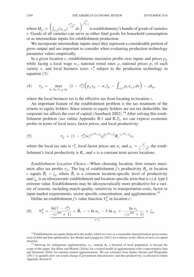
2590 THE AMERICAN ECONOMIC REVIEW SEpTEMbER 2016
where M jc ≡ ( ∫ v∈J ( x v, jc )
ε PD +1 ____ ε PD
dv)
ε PD _ ε PD +1
is establishment j ’s bundle of goods of varieties v . Goods of all varieties can serve as either final goods for household consumption or as intermediate inputs for establishment production.
We incorporate intermediate inputs since they represent a considerable portion of gross output and are important to consider when evaluating production technology parameter values empirically.
In a given location c , establishments maximize profits over inputs and prices p jc while facing a local wage w c , national rental rates ρ , national prices p v of each variety v , and local business taxes τ c b subject to the production technology in equa tion (3):
(4) π jc = max l jc , k jc , x v, jc , p jc
(1 − τ c b ) ( p jc y jc − w c l jc − ∫ v∈J
p v x v, jc dv) − ρ k jc ,
where the local business tax is the effective tax from locating in location c .An important feature of the establishment problem is the tax treatment of the
returns to equity holders. Since returns to equity holders are not tax deductible, the corporate tax affects the cost of capital (Auerbach 2002).14 After solving this estab-lishment problem (see online Appendix B.1 and B.2), we can express economic profits in terms of local taxes, factor prices, and local productivity:
(5) π jc = (1 − τ c b ) w c γ( ε PD +1) ρ c δ( ε PD +1) B c −( ε PD +1) κ,
where the local tax rate is τ c b , local factor prices are w c and ρ c = ρ _ 1 − τ c b
, the estab-
lishment’s local productivity is B c , and κ is a constant term across locations.
Establishment Location Choice.—When choosing location, firm owners maxi-mize after tax profits π jc . The log of establishment j ’s productivity B jc in location c equals B ̅ c + ζ jc where B ̅ c is a common location-specific level of productivity and ζ jc is an idiosyncratic establishment and location-specific term that is i.i.d. type I extreme value. Establishments may be idiosyncratically more productive for a vari-ety of reasons, including match-quality, sensitivity to transportation costs, factor or input market requirements, sector-specific concentration, and agglomeration.15
Define an establishment j ’s value function V jc F in location c :
(6) V jc F = ln (1 − τ c b ) _
−( ε PD + 1) + B ̅ c − γ ln w c − δ ln ρ c + ln κ 1 _
−( ε PD + 1)
≡ v c
+ ζ jc .
14 Establishments are equity financed in the model, which we view as a reasonable characterization given nontax costs of debt and firm optimization. See Heider and Ljungqvist (2015) for evidence on the effects of taxes on capital structure.
15 Allowing for endogenous agglomeration, i.e., making B jc a function of local population, is beyond the scope of this paper. See Kline and Moretti (2014a) for a related model of agglomeration with a representative firm and Diamond (2016) for amenity-related agglomerations. We use estimates from Suárez Serrato and Wingender (2011) to quantify how our results change if government infrastructure (and thus productivity) is affected in online Appendix Section F.

2591SuÁrez Serrato and zidar: BenefitS from State Corporate tax CutSVoL. 106 no. 9
This value function is a positive monotonic transformation of log profits.16
Similar to the household location problem, establishments will locate in location c if their value function there is higher than in any other location c ′. The share of establishments for which that is true determines local establishment share E c :
(7) E c = P ( V jc = max c′ { V j c ′ }) =
exp v c _ σ F
_______
∑ c′ exp v c′ __ σ F
,
where σ F is the dispersion of the location-specific idiosyncratic establishment pro-ductivity ζ jc .
Local Labor Demand.—Local labor demand depends on the share of establish-ments that choose to locate in c as well as the average employment of local firms and is given by the following expression:17
(8) L c D = E c × E ζ [ l jc ∗ ( ζ jc ) |c = arg max
c′ { V j c ′ }]
= ( 1 _ C π ̅
exp ( v c _ σ F
) )
Extensive margin
× w c (γ ε PD +γ−1) ρ c (1+ ε PD )δ κ 0 ( e B ̅ c (− ε PD −1) ) z c
Intensive margin
,
where C is the number of cities, π ̅ ≡ 1 _ C ∑ c′ exp ( v c′ __ σ F
) is closely related to average
profits in all other locations, κ 0 is a common term across locations, and z c is a term increasing in the idiosyncratic productivity draw ζ jc . From this equation we obtain a key object of interest for incidence: the macro elasticity of local labor demand,
(9) ∂ ln L c D _ ∂ ln w c = γ − 1 ⏟
Substitution
+ γ ε PD ⏟
Scale
− γ _ σ F
⏟
Firm−Location
≡ ε LD ,
where γ is the output elasticity of labor, ε PD is the product demand elasticity, and σ F is the dispersion of idiosyncratic productivity.
This expression is labeled the macro elasticity of labor demand because it com-bines the average firm’s elasticity plus the effect of firm entry on labor demand.
16 The transformation divides log profits by −( ε PD + 1) ≥ 1 , where log profits are the nontax shifting portion of log profits, i.e., ln π jc = ln (1 − τ i A ) + γ ( ε PD + 1) ln w c + δ ( ε PD + 1) ln ρ c − ( ε PD + 1) ln B ̅ c + ln κ 1 , which closely approximates the exact expression for log profits as shown in online Appendix B.2.2. Note that − ( ε PD + 1) −1 = μ − 1 , which is the net-markup.
17 Given a large number of cities C , we can follow Hopenhayn (1992) and use the law of large numbers to sim-
plify the denominator of E c and express the share E c = ( exp
v c __ σ F
____ C π ̅
) as a function of average location-specific profits
in all other locations π ̅ ≡ 1 _ C ∑ c′ exp ( v c′ __ σ F
) .

2592 THE AMERICAN ECONOMIC REVIEW SEpTEMbER 2016
In addition, this equation also yields our last key object of interest: the effect of a business tax change on local labor demand, which is given by
∂ ln L c D _ ∂ ln (1 − τ c b )
= ∂ ln E c _ ∂ ln (1 − τ c b )
= 1 ___________ −( ε PD + 1) σ F
= μ − 1 _
σ F ,
where the last equation uses the definition of the net-markup: μ − 1 .
II. The Incidence of Local Corporate Tax Cuts
We characterize the incidence of corporate taxes on wages, rents, and profits and relate these effects to the welfare of workers, landowners, and firms. We focus on the welfare of local residents as the policies we study are determined by policymakers with the objective of maximizing local welfare.
A. Local Incidence on Prices and Profits
Assuming full labor force participation, i.e., L c S = N c , clearing in the housing, labor, capital, and goods markets gives the following labor market equilibrium:
N c ( w c , r c ; A ̅ c , η c ) = L c D ( w c , π ̅ ; ρ c , τ c b , B ̅ c , z c ) .
This expression implicitly defines equilibrium wages w c . Let w ̇ c = d ln w c _ d ln (1 − τ c b )
and
define r ̇ c analogously. The effects of a local corporate tax cut on local wages, rents, and after-tax profits are given by the following expressions:
(10) w ̇ c = ( ∂ ln L c D _
∂ ln (1 − τ c b ) ) ___________
ε LS − ε LD =
(μ − 1) _
σ F ___________________________
( 1 + η c − α _ σ W (1 + η c ) + α
) − γ ( ε PD + 1 − 1 _ σ F
) + 1 , and
(11) r ̇ c = ( 1 + ε LS _ 1 + η c
) w ̇ c .
(12) π ̇ c = 1 −δ ( ε PD + 1)
Reducing capital wedge
+ γ ( ε PD + 1) w ̇ c
Higher labor costs
,
where π ̇ c is the percentage change in after-tax profits, δ is the output elasticity of capital, ε PD is the product demand elasticity, γ is the output elasticity of labor, and w ̇ c is the percentage change in wages following a corporate tax cut.
Discussion.—The expression for wage growth in equation (10) has an intuitive economic interpretation that translates the forces in our spatial equilibrium model to those in a basic supply and demand diagram, as in Figure 1. The numerator captures
the shift in labor demand following the tax cut: (μ − 1) _
σ F . Since this shift in demand

2593SuÁrez Serrato and zidar: BenefitS from State Corporate tax CutSVoL. 106 no. 9
Figure 1. The Impact of a Corporate Tax Cut on Workers and Firm Owners
Notes: Panel A: Monopolistically competitive establishments earn profits, which are divided into taxes and after-tax profits. Panel B: Cutting corporate taxes has three effects on local establishments: a corporate tax cut reduces the establishment’s (1) tax liability and (2) capital wedge mechanically. (3) Establishments enter the local area and bid up wages by w ̇ percent.
I. Effects on each local establishment
Panel A. Before tax cut
DMR
Dol
lars
y
Dol
lars
y
MC0
p0
MC0
MC′
p0
Panel B. A corporate tax cut has 3 effects
∝ w
D
.
1
23
MR
(Continued)

2594 THE AMERICAN ECONOMIC REVIEW SEpTEMbER 2016
II. Equilibrium effects on local wages and after-tax pro�ts
Panel C. Wage increase determined in labor market
w0
L
=
∆D
Panel D. Net effect on after-tax pro�ts
y
L0
D0
S0
L′
D′
ƐLS − ƐLD
w.
w. ∆(1 − τ)
Dol
lars
w0
MC0
D
p′
MC′ w. ∝
Wag
e w′
Figure 1. The Impact of a Corporate Tax Cut on Workers and Firm Owners (Continued)
Notes: Panel C: Wage increases are determined in the local labor market as workers move in, house prices increase, each establishment hires fewer workers, and some marginal establishments leave. Panel D: The cumulative per-centage increase on profits π ˙ depends on the magnitude of wage increases. We derive the change in local labor demand, ε LS , and ε LD from microfoundations and express them in terms of a few estimable parameters in Section I. Empirical estimates of these parameters, which govern the three effects above are provided in Table 6 and online Appendix Table A33 and discussed in Section VI. Note that these effects are enumerated to help provide intuition, but the formal model does not include dynamics. The model shows how the spatial equilibrium changes when states cut corporate taxes.

2595SuÁrez Serrato and zidar: BenefitS from State Corporate tax CutSVoL. 106 no. 9
is due to establishment entry, the numerator is a function of the location decisions of establishments. Profit taxes matter more for location decisions when markups (and thus profits) are large, but matter less when productivity is more heteroge-neous across locations. The denominator is the difference between an effective labor supply elasticity and a macro labor demand elasticity. The effective elasticity of
labor supply ε LS = ( 1 + η c − α _ σ W (1 + η c ) + α
) incorporates indirect housing market impacts.
As ∂ ε LS _ ∂ η c > 0 , the effect of corporate taxes on wages will be smaller, the larger the
elasticity of housing supply. A simple intuition for this is that if η is large, work-ers do not need to be compensated as much to be willing to live there. As shown in equation (9), the elasticity of labor demand depends on both location and scale decisions of firms.
In the expression for rental costs in equation (11), the quantity 1 + ε LS captures the effects of higher wages on housing consumption through both a direct effect of higher income and an indirect effect on the location of workers. The magnitude of the rent increase depends on the elasticity of housing supply η c and the strength of the inflow of establishments through its effect on w ̇ c as in equation (10).
Equation (12) shows that establishment profits mechanically increase by 1 per-cent following a corporate tax cut of 1 percent. They are also affected by effects on factor prices. The middle term reflects increased profitability due to a reduction in the effective cost of capital. The last term shows that, as firms enter the local labor market, wages rise and thus compete away profits.
B. Local Incidence on Welfare
Having derived the incidence of corporate taxes on local prices and profits, we now explore how these price changes affect the welfare of workers, landowners, and firm owners.
We define the welfare of workers as W ≡ E [ma x c { u c + ξ nc } ] . Since the distri-bution of idiosyncratic preferences is type I extreme value, the welfare of workers can be written as
W = σ W log ( ∑ c exp ( u c _
σ W ) ) ,
as in McFadden (1978) and Kline and Moretti (2014b).It then follows that the effect of a tax cut in location c on the welfare of workers
is given by
(13) d W _ d ln (1 − τ c c ) = N c ( w ̇ c − α r ̇ c ) .
That is, the effect of a tax cut on welfare is simply a transfer to workers in loca-tion c equivalent to a percentage change in the real wage given by ( w ̇ c − α r ̇ c ) . One very useful aspect of this formula is that it does not depend on the effect of tax changes on the location decisions of workers in the sense that there are no N ̇ c terms in this expression (Busso, Gregory, and Kline 2013).

2596 THE AMERICAN ECONOMIC REVIEW SEpTEMbER 2016
This expression assumes d W _ d ln (1 − τ c b )
= d c W _ d ln (1 − τ c b )
, that is, tax changes in location
c have no effect on wages and rental costs in other locations, consistent with the perspective of a local official.
Similarly, defining the welfare of firm owners as18
F ≡ E [ max c { v c + ζ jc } ] × −( ε PD + 1)
yields an analogous expression for the effect of corporate taxes on domestic firm owner welfare:
(14) d F _ d ln (1 − τ c c ) = E c π ̇ c .
Finally, consider the effect on landowner welfare in location c . Landowner wel-fare in each location is the difference between housing expenditures and the costs associated with supplying that level of housing. This difference can be expressed as follows:19
L = N c α w c − ∫ 0 N c α w c / r c G −1 (q; Z c h ) dq = 1 _
1 + η c N c α w c ,
and is proportional to housing expenditures. The effect of a corporate tax cut on the welfare of domestic landowners is then given by
(15) d L _ d ln (1 − τ c c ) = N ̇ c + w ̇ c _
1 + η c .
III. Empirical Implementation and Identification
This section describes how we connect the theory to the data to implement the incidence formulae from the previous section. We write the key equations of the spa-tial equilibrium model from Section I as a simultaneous equations model and show that there is an associated exact reduced-form that relates equilibrium changes in the number of households, firms, wages, and rental prices to the structural parameters of the model. We then show that the incidence formulae are identified by simple combinations of these equilibrium responses, which can also be used to recover the key structural parameters of the model.
18 The firm owner term is multiplied by −( ε PD + 1) > 0 to undo the monotonic transformation in definition of the establishment value function V jc F . Firm owners and landlords are distinct from workers for conceptual clarity.
19 Note that, in contrast to workers and firm owners, this formulation of the utility of the representative land-lord assumes constant marginal utility of income. In addition, rising rents may reflect increases in wages that do not accrue directly to landowners. Direct data on land values (e.g., Albouy and Ehrlich 2012) could improve this measurement.

2597SuÁrez Serrato and zidar: BenefitS from State Corporate tax CutSVoL. 106 no. 9
A. Exact Reduced-Form Effects of Business Tax Changes
The simultaneous equation model is given by the log-labor supply equation (equa-tion (1)), the log-value of equilibrium rents (equation (2)), the log of the establish-ment location equation (equation (7)), and the log-labor demand equation (equation (8)). To economize on the number of parameters, we set η c = η ∀ c . Stacking these equations yields the structural form:
(16) A Y c, t = B Z c, t + e c, t ,
where Y c, t is a vector of the four endogenous variables (wage growth, population growth, rental cost growth, and establishment growth), Z c, t = [ Δ ln (1 − τ c, t b ) ] is a vector of tax shocks, A is a matrix that characterizes the inter-dependence among the endogenous variables, B is a matrix that measures the direct effects of the tax shocks on each endogenous variable, and e c, t is a structural error term. Explicitly, these elements are given by
Y c, t =
⎡
⎢ ⎣
Δln w c, t
Δln N c, t Δln r c, t
Δln E c, t
⎤
⎥ ⎦
, A =
⎡
⎢ ⎣
− 1 _ σ W
1
α _ σ W
0
1
− 1 _ ε LD
0
0
− 1 _ 1 + η
− 1 _ 1 + η
1
0
γ _ σ F
0
0
1
⎤
⎥ ⎦
, B =
⎡
⎢ ⎣
0
1 _ ε LD σ F ( ε PD + 1)
0
1 _ − σ F ( ε PD + 1)
⎤
⎥ ⎦
.
Pre-multiplying by the inverse of the matrix of structural coefficients A gives the reduced form:
(17) Y c, t = A −1 B ⏟
≡ β Business Tax Z c, t + A −1 e c, t ,
where β Business Tax is a vector of reduced-form effects of business tax changes:
β Business Tax =
⎡
⎢ ⎣
β W
β N β R
β E
⎤
⎥ ⎦
=
⎡
⎢ ⎣
w ̇
w ̇ ε LS
1 + ε LS _ 1 + η w ̇
μ − 1 _
σ F − γ _
σ F w ̇
⎤
⎥ ⎦
.
The expressions in the exact reduced form have insightful intuitive economic interpretations. The observed equilibrium change in wages and rents, β W and β R , are given by the incidence equations (10) and (11). The equilibrium change in employ-ment, β N , is given by the change in wage multiplied by the effective elasticity of labor supply. The change in the number of establishments, β E , is determined by
two forces. The first, μ − 1 _
σ F , is the increase in the number of establishments that

2598 THE AMERICAN ECONOMIC REVIEW SEpTEMbER 2016
would occur if wages did not change. The second component accounts for the equi-librium change in wages. Higher wages decrease the number of establishments by − γ _
σ F w ̇ .
B. Identification of Parameters and Incidence Formulae
This section shows that these four reduced-form moments, β Business Tax = [ β W , β N , β R , β E ] ′ , are sufficient to identify the incidence on the wel-fare of each of our agents, up to the calibration of expenditure share α and output elasticity ratio δ/γ . Table 1 reproduces the incidence formulae for the welfare of each of our agents. The direct effects of taxes on disposable income ( β W − α β R ) and on rents β R identify the impacts on workers and landowners, respectively. The expression for firm owners depends on the equilibrium effect on profits, which are not directly observed empirically.
Table 1 shows that the formula for the incidence on after-tax profits includes the term γ ( ε PD + 1) . This term measures the decrease in profits from a 1-percent increase in wages normalized by the firm’s net-markup.
Intuitively, the amount firms care about wage changes depends on how much wage changes impact their costs, which is governed by γ , and how much firms have to scale back production when costs are higher, which is governed by the product demand elasticity. We identify γ ( ε PD + 1) by inverting the wage incidence equation.
We recover the elasticity of labor supply, which is identified by the ratio of the first two rows of equation (17) so that ε LS = β N / β W . Similarly, the shift in labor demand is given by rearranging the establishment location in the last row of equa-tion (17),
μ − 1 _
σ F = β E + γ _
σ F β W .
Table 1—Identification of Local Incidence on Welfare and Structural Parameters
Stakeholder (benefit) Incidence Identified by
Panel A. Local incidenceWorkers (disposable income)
w ̇ − α r ̇ β W − α β R
Landowners (housing costs)
r ̇ β R
Firm owners (after-tax profit)
1 + γ ( ε PD + 1) ( w ̇ c − δ _ γ ) 1 + ( β N − β E _ β W
+ 1) ( β W − δ _ γ )
Panel B. Structural parametersWorker mobility Firm mobility Housing supply Product demand
σ W = β W − α β R _ β N
σ F = γ β W _ β E
( 1 _ β E − β N − β W
− 1) η = β N + β W _ β R
− 1 ε PD = β N + β W − β E _ γ β W
Notes: This table shows how reduced-form estimates β Business Tax = [ β W , β N , β R , β E ] ′ map to the incidence on wel-fare of workers, landowners, and firm-owners at the local level. Note that we calibrate the housing expenditure share ( α ) and the ratio of the capita to labor output elasticities ( δ/γ ).

2599SuÁrez Serrato and zidar: BenefitS from State Corporate tax CutSVoL. 106 no. 9
This equation states that the shift in labor demand is given by the observed change in the number of establishments, β E , plus the number of establishments that would
have entered had wages not risen, as given by γ _ σ F
β W . Expressing the wage incidence
formula as a function of reduced-form parameters yields
(18) β W = β E + γ _
σ F β W _____________________
β N _ β W
− γ ( ε PD + 1 − 1 _ σ F
) + 1
ε LD
.
Solving equation (18) for γ ( ε PD + 1) shows that it is identified by the following combination of reduced-form moments:
γ ( ε PD + 1) = ( β N − β E _ β W
+ 1) .
The intuition behind this derivation is that, given estimates of the equilibrium change in wages, employment, and the slope of labor supply, we can decompose the elasticity of labor demand into the extensive component, using the equilibrium change in establishments, and the remaining intensive margin γ ( ε PD + 1) − 1 . This micro-elasticity of labor demand also reveals the effect of a wage increase on profits, which determines the incidence on firm owners.
A few remarks are worth highlighting about this identification argument. First, given α and δ/γ , the welfare effects are point identified even though we cannot identify all seven model parameters with four moments. In particular, even though we cannot separately identify γ and ε PD , identifying the product γ ( ε PD + 1) is suf-ficient to characterize the effect of a corporate tax cut on profits. Second, we can fur-ther identify additional primitives of the model including σ W and η c by manipulating the identification of the elasticity of labor supply and the incidence on rents. Table 1 presents formulae for each of the structural parameters we estimate as functions of the four reduced-form moments and calibrated parameters α and γ . Third, this iden-tification argument highlights the relationship between the model and reduced-form estimates, providing a transparent way to evaluate how sensitive our ultimate inci-dence estimates are to changes in the four reduced-form estimates. Finally, in some specifications we augment this model to include the effects of personal income taxes on housing supply and worker location as well as the effects of observable productivity shocks due to Bartik (1991) on the local labor market equilibrium.20 For brevity, we relegate discussion of the exact reduced-from expressions to online Appendix E.5. However, note that the reduced-form identification argument above is not affected by the inclusion of additional sources of variation.
20 In particular, the location decision of workers is modified by replacing w with after tax income w (1 − τ i ) and the supply of housing now becomes H c S = (1 − τ i ) χ H ( B c H r c ) η c , where the parameter χ H is estimated in the cases where we estimate the system using the variation from all shocks. Note that, additionally, one could also incorporate local property taxes by including property taxes in the cost of housing in the worker location equation.

2600 THE AMERICAN ECONOMIC REVIEW SEpTEMbER 2016
IV. Data and Institutional Details of State Corporate Taxes
We use annual county-level data from 1980–2012 for over 3,000 counties and decadal individual-level data to create a panel of outcome and tax changes for 490 county groups. Ruggles et al. (2010) developed and named these county-groups “consistent public-use micro-data areas (PUMAs).” This level of aggregation is the smallest geographical level that can be consistently identified in census and American Community Survey (ACS) datasets and provides several benefits (see online Appendix A.1).
A. Data on Economic Outcomes
We aggregate the number of establishments in a given county to the PUMA county groups using data from the Census Bureau’s County Business Patterns (CBP). We analogously calculate population changes using Bureau of Economic Analysis (BEA) data.
Data on local wages and housing costs are available less frequently. We use individual-level data from the 1980, 1990, and 2000 US censuses and the 2009 ACS to create a balanced panel of 490 county groups with indices of wages, rental costs, and housing values.
When comparing wages and housing values, it is important that our comparisons refer to workers and housing units with similar characteristics. As is standard in the literature on local labor markets, we create indices of changes in wage rates and rental rates that are adjusted to eliminate the effects of changes in the compositions of workers and housing units in any given area.
We create these composition-adjusted values as follows. First, we limit our sam-ple to the nonfarm, noninstitutional population of adults between the ages of 18 and 64. Second, we partial out the observable characteristics of workers and housing units from wages and rental costs to create a constant reference group across loca-tions and years. We do this adjustment to ensure that changes in the prices we ana-lyze are not driven by changes in the composition of observable characteristics of workers and housing units. Additional details regarding our sample selection and the creation of composition-adjusted outcomes are available in online Appendix A.2. Finally, we construct a “Bartik” local labor demand shock that we use to supplement our tax change measure and enhance the precision of labor supply parameters.21
21 This approach weights national industry-level employment shocks by the initial industrial composition of each local area to construct a measure of local labor demand shocks:
Barti k c, t ≡ ∑ Ind
EmpShar e Ind, t−10, c × ΔEm p Ind, t, US ,
where EmpShar e Ind, t−10, c is the share of employment in a given industry at the start of the decade and ΔEm p Ind, t, US is the national percentage change in employment in that industry. We calculate national employment changes as well as employment shares for each county group using micro-data from the 1980, 1990, and 2000 censuses and the 2009 ACS. We use a consistent industry variable based on the 1990 census that is updated to account for changes in industry definitions as well as new industries.

2601SuÁrez Serrato and zidar: BenefitS from State Corporate tax CutSVoL. 106 no. 9
B. Tax Data
Businesses pay two types of income taxes. C-corporations pay state corporate taxes and many other types of businesses, such as S-corporations and partnerships, pay individual income taxes. We combine these measures to calculate an average business tax rate for each local area from 1980 to 2010.
State Corporate Tax Data and Institutional Details.—The tax rate we aim to obtain in this subsection is the effective average tax rate paid by establishments of C-corporations in a given location from 1980 to 2010. Firms can generate earnings from activity in many states. State authorities have to determine how much activity occurred in state s for every firm i . They often use a weighted average of payroll, property, and sales activity. The weights θ s , called apportionment weights, deter-mine the relative importance tax authorities place on these three measures of in-state activity.22 From the perspective of the firm i , the firm-specific “apportioned” tax rate is a weighted average of state corporate tax rates:
(19) τ i A = ∑ s τ s c ω is ,
where τ s c is the corporate tax rate in state s and the firm-specific weights ω is are
themselves weighted averages ω is = ( θ s w W is _ W )
⏟
payroll
+ ( θ s ρ R is _ R )
⏟
property
+ ( θ s x X is _ X )
⏟
sales
of in-state
activity shares.23 Equation (19) shows that the tax rate corporations pay depends on home-state and other states’ tax rates and rules. We use the latter to construct an external rate τ i E , which represents an index of the importance of changes in every other state’s tax and yields variation that is likely exogenous to local economic con-ditions. It is defined explicitly in online Appendix A.3.1.
To implement the activity shares for each firm i , we use the Reference USA dataset from Infogroup to compute the geographic distribution of payroll at the firm level. Due to the lack of information on the geographic distribution of property in the Reference USA dataset, we make the simplifying assumption that capital activ-ity weights equal the payroll weights. Finally, since the apportionment of sales is destination-based, we use state GDP data for ten broad industry groups from the BEA to apportion sales to states based on their share of national GDP.24
Empirically, we use the spatial distribution of establishment-firm ownership and payroll activity in 1997, the first year in which micro establishment-firm linked data
22 Goolsbee and Maydew (2000) use variation in apportionment weights on payroll activity to show that reduc-ing the payroll weight from 33 percent to 25 percent leads to an increase in manufacturing employment of roughly 1 percent on average. In addition, we follow their approach of analyzing the determinants of state tax policy changes by estimating a probit of the likelihood that a state has a tax policy change based on how observable economic and tax policy conditions such as state per capita income growth, state corporate tax rates, state income tax rates, and the apportionment weights of other states relate to apportionment formula and tax rate policy changes. The results, which are discussed in online Appendix A.6, are in online Appendix Tables A34 and A35.
23 In particular, a is w ≡ W is _ W is the payroll activity share. Payroll and sales shares are defined analogously. See online Appendix A.3.1 for more detail on apportionment rules.
24 This assumption corresponds to the case where all goods are perfectly traded, as in our model. We use broad industry groups in order to link SIC and NAICS codes when calculating GDP by state-industry-year.

2602 THE AMERICAN ECONOMIC REVIEW SEpTEMbER 2016
are available. We hold the spatial distribution of establishment-firm ownership and payroll activity weights constant at these initial values to avoid endogenous changes in effective tax rates. Consequently, variation in our tax measure τ i A comes from variation in state apportionment rules, variation in state corporate tax rules, and ini-tial conditions, which determine the sensitivity of each firm’s tax rate τ i A to changes in corporate rates and apportionment weights. We combine our empirical activity share measures with state corporate tax rates and apportionment rules from Book of the States, Significant Features of Fiscal Federalism, and Statistical Abstracts of the United States.
We then use these components to compute an average tax rate τ ̅ c A for all establish-ments in each location and decompose it into average local “domestic” and external rates, τ ̅ c D and τ ̅ c E .
Figure 2 shows that apart from a few states that have never taxed corporate income, most states have changed their rates at least three times since 1979. Online Appendix Figure A3 shows how large these rate changes have been over a 30 year
Panel A. Number of corporate tax changes by state since 1979
Panel B. Corporate tax rates by state in 2012
(5,9](3,5](1,3][0,1]Never tax
(8.5,12](7.5,8.5](6,7.5][0,6]Never tax
Figure 2. State Corporate Tax Rates
Notes: These figures show statistics on state statutory corporate tax rates across states. See online Appendix Figures A2, A3, A4, and A5 for similar figures on state corporate tax apportionment rates, 30 year changes in cor-porate rates and apportionment rules, state establishment and population shares, and 30 year changes in establish-ment and population shares, respectively.

2603SuÁrez Serrato and zidar: BenefitS from State Corporate tax CutSVoL. 106 no. 9
period from 1980–2010. States in the South made fewer changes while states in the Midwest and Rust Belt changed rates more frequently. This figure shows that changes in state corporate tax rates did not come from a particular region of the United States. State corporate tax changes are not only frequent, but they can also be sizable. Of the 1,470 PUMA-decade observations in the main dataset, there are hundreds of sizable changes in both aspects of corporate tax policy over three peri-ods of interest: 1980–1990, 1990–2000, and 2000–2010.25
States also vary in the apportionment rates that they use. Table 2 provides sum-mary statistics of apportionment weights. Since the late 1970s, apportionment weights generally placed equal weight on payroll, property, and sales activity, set-ting θ s w = θ s ρ = θ s x = 1 _ 3 . For instance, 80 percent of states used an equal-weighting
25 Specifically, online Appendix Figure A6 shows a histogram of nonzero tax changes in corporate tax rates in panel A and in payroll apportionment rates in panel B.
Table 2—Summary Statistics
Variable Mean SD Min Max Observations
Annual outcome data from BEA and CBPYear 1995 8.9 1980 2010 15,190log population: ln N c, t 13.8 1.1 10.9 16.1 15,190log employment: ln L c, t 13.2 1.2 9.4 15.6 15,190log establishments: ln E c, t 10.0 1.2 6.5 12.4 15,190
Annual data on apportionment rules and corporate, personal, and business tax ratesState corporate tax apportionment parameters Payroll apportionment weight: θ s, t w 22.7 11.6 0.0 33.3 15,190 Property apportionment weight: θ s, t ρ 22.8 11.6 0.0 33.3 15,190 Sales apportionment weight: θ s, t x 54.5 23.2 25 100 15,190
Corporate income Rate: τ s, t c 6.6 3.0 0.0 12.3 15,190 Percent change in net-of-rate: −0.01 0.4 −5.4 3.8 15,190 Δln (1 − τ c ) s, t, t−1 Personal income Effective rate: τ s, t i 2.6 1.7 0.0 7.4 15,190 Percent change in net-of-rate: 0.03 0.2 −3.3 2.5 15,190 Δln (1 − τ i ) s, t, t−1 Business income Rate: τ c, t b 3.1 1.1 0.3 5.4 15190 Percent change in net-of-rate: −0.01 0.2 −1.8 1.2 15,190 Δln (1 − τ b ) c, t, t−1
Year 2000 8.2 1990 2010 1,470Decadal dataPercentage change in: Population: Δln N c, t, t−10 11.2 10.4 −16.6 76.1 1,470 Establishments: Δln E c, t, t−10 15.2 16.5 −23 126.2 1,470 Adjusted wages: Δln w c, t, t−10 −2.8 7.2 −31.2 14.9 1,470 Adjusted rents: Δln r c, t, t−10 8.5 12.0 −41.4 43.4 1,470 Net-of-corp.-rate: Δln (1 − τ c ) s, t, t−10 −0.1 1.1 −5.4 4.5 1,470 Net-of-pers.-rate: Δln (1 − τ i ) s, t, t−10 −1.3 1.1 −5.3 1.3 1,470 Net-of-bus.-rate: Δln (1 − τ b ) c, t, t−10 −0.8 0.6 −2.8 1.3 1,470 Gov. expend./capita: Δln G c, t, t−10 0.0 0.6 −13.3 11.6 1,470
Bartik shock: Bartik c, t, t−10 7.8 4.8 −15.2 26.0 1,470
Sources: BEA, CBP, Zidar (2016), Suárez Serrato and Wingender (2011) corporate tax sources in Section IV
2604 THE AMERICAN ECONOMIC REVIEW SEpTEMbER 2016
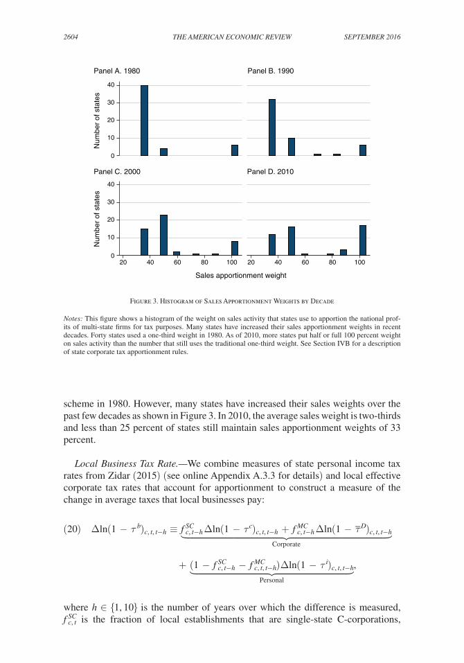
scheme in 1980. However, many states have increased their sales weights over the past few decades as shown in Figure 3. In 2010, the average sales weight is two-thirds and less than 25 percent of states still maintain sales apportionment weights of 33 percent.
Local Business Tax Rate.—We combine measures of state personal income tax rates from Zidar (2015) (see online Appendix A.3.3 for details) and local effective corporate tax rates that account for apportionment to construct a measure of the change in average taxes that local businesses pay:
(20) Δln (1 − τ b ) c, t, t−h ≡ f c, t−h SC Δln (1 − τ c ) c, t, t−h + f c, t−h MC Δln (1 − τ ̅ D ) c, t, t−h
Corporate
+ (1 − f c, t−h SC − f c, t, t−h MC ) Δln (1 − τ i ) c, t, t−h
Personal
,
where h ∈ {1, 10} is the number of years over which the difference is measured, f c, t SC is the fraction of local establishments that are single-state C-corporations,
0
10
20
30
40
0
10
20
30
40
20 40 60 80 100 20 40 60 80 100
Panel A. 1980 Panel B. 1990
Panel C. 2000 Panel D. 2010
Num
ber
of s
tate
sN
umbe
r of
sta
tes
Sales apportionment weight
Figure 3. Histogram of Sales Apportionment Weights by Decade
Notes: This figure shows a histogram of the weight on sales activity that states use to apportion the national prof-its of multi-state firms for tax purposes. Many states have increased their sales apportionment weights in recent decades. Forty states used a one-third weight in 1980. As of 2010, more states put half or full 100 percent weight on sales activity than the number that still uses the traditional one-third weight. See Section IVB for a description of state corporate tax apportionment rules.

2605SuÁrez Serrato and zidar: BenefitS from State Corporate tax CutSVoL. 106 no. 9
and f c, t MC is the fraction of local establishments that are multi-state C-corporations.26 While this measure captures several key features of local business taxation, we made a number of simplifying assumptions in generating τ b due to data limitations and feasibility.27
We discuss these assumptions and tax measurement details in online Appen-dix A.3.4. Overall, changes in corporate tax rates, apportionment weights, and per-sonal income tax rates generate considerable variation in effective tax rates across time and space. Table 2 provides summary statistics of a few different measures of corporate tax changes over ten-year periods. The average log change over ten years in corporate taxes due only to statutory corporate rates Δln (1 − τ c ) c, t, t−10 is near zero and varies less than measures based on business taxes that incorporate the com-plexities of apportionment changes. Business tax changes Δln (1 − τ b ) c, t, t−10 are slightly more negative on average over a ten-year period. The minimum and max-imum values are less disperse than the measure based on statuary rates since sales apportionment reduces location-specific changes in effective corporate tax rates. Overall, 76 percent of the variation in Δln (1 − τ b ) c, t, t−10 is due to policy variation (changes in tax rates and apportionment rules).
C. Calibrated Parameters
We calibrate two parameters when implementing the reduced-form formulae in Table 1: the ratio of the capita to labor output elasticities ( δ/γ ) and the hous-ing expenditure share ( α ). We use 0.9 for the ratio of output elasticities based on data from the Bureau of Economic Analysis. BEA’s 2012 data on shares of gross output by industry indicate that for private industries, compensation and inter-mediate inputs account for 28.5 percent and 45.6 percent respectively; the ratio
1 − 0.285 − 0.456 ___________ 0.285
≈ 0.9 . Our baseline results use α = 0.3 , which we obtain using
data from the Consumer Expenditure Survey (CEX).28 We calibrate two additional parameters for the structural estimation: the output elasticity of labor γ and the prod-uct demand elasticity ε PD . We present results for calibrations for wide ranges of both parameters. We choose a baseline of γ = 0.15 , which is close to other val-ues used in the local labor markets literature (e.g., Kline and Moretti 2014a use 1 − α − β = 1 − 0.3 − 0.47 = 0.23 in their notation) and is based on cost shares from IRS and BEA.29 For our baseline ε PD , we use values that are slightly lower than in the macro and trade literatures (e.g., Coibion, Gorodnichenko, and Wieland
26 These shares are from County Business Patterns and RefUSA. C-corps accounted for roughly half of employ-ment and one-third of establishments in 2010. Yagan (2015) notes that switching between corporate types is rare empirically.
27 For instance, partnerships and sole-proprietors pay taxes based on the location of the owner and not the establishment. For simplicity, we assume that owners of pass-through entities are located in the same state as the establishment. Additionally, using aggregated-average rates is not directly justified by the model, so our estimates are approximations.
28 Similar values of this parameter are used by Notowidigdo (2013) and Suárez Serrato and Wingender (2011) and, as Moretti (2013) notes, the Bureau of Labor and Statistics uses a cost share of 32 percent for shelter. However, we consider larger values as well because Albouy (2008) and Moretti (2013) note that housing prices are related to nonhousing “ home-goods” which increases the effective cost share and Diamond (2016) also estimates a higher value of this parameter.
29 The IRS SOI data are from the most recent year available (2003) and can be downloaded at http://www.irs.gov/uac/ SOI-Tax-Stats-Integrated-Business-Data. These data show that costs of goods sold are substantially larger

2606 THE AMERICAN ECONOMIC REVIEW SEpTEMbER 2016
2012; Arkolakis et al. 2013) in order to obtain ε LD values that are closer to those used in the labor literature (Hamermesh 1993). We also provide specifications in which we estimate ε PD directly.
Table 3 summarizes our choices for calibrated parameters as well as references for each parameter. Our baseline values are presented in bold and we also include alternative values that we consider in order to explore the robustness of our results. We also make other implicit calibrations from our modeling of preferences and tech-nologies. In preferences, the income elasticity and elasticity of substitution for hous-ing are both set to one. These assumptions result in a constant share of expenditure on housing, α , which yields a constant elasticity of labor supply, ε LS . In terms of technologies, the production function has constant returns to scale and unit elasticity of substitution among capital, labor, and intermediate goods. This setup affects the scale and substitution components in equation (8) and thus the elasticity of labor demand, ε LD .
V. Reduced-Form Results and Incidence Estimates
We use changes in state tax rates and apportionment formulas to estimate the reduced-form effects of local business tax changes on population, the number of establishments, wages, and rents. We estimate equation (17) for a given outcome Y as the first-difference over a ten-year period:
(21) ln Y c, t − ln Y c, t−10 = β Y [ln (1 − τ c, t b ) − ln (1 − τ c, t−10 b ) ] + D s, t ′ Ψ s, t LD + u c, t ,
where ln Y c, t − ln Y c, t−10 is approximately outcome growth over ten years, [ln (1 − τ c, t b ) − ln (1 − τ c, t−10 b ) ] is the change in the net-of-business-tax-rate over ten years, and D s, t is a vector with year dummies as well as state dum-mies for states in the industrial Midwest in the 1980s, and where a county-group
than labor costs and that Salaries and Wages ________________ Salaries and Wages + COGS = 0.153 . Results based on revenue and cost shares from earlier
years available are similar. BEA data on gross output for private industries show similar patterns as well.
Table 3—Calibrated Parameters used in Incidence Formulae
Parameter Values Sources
Parameters for reduced-form implementationRatio of elasticities: γ/δ {0.90, 0.50, 0.75} BEAHousing cost share: α {0.30, 0.50, 0.65} CEX, Albouy (2008), Moretti (2013)
Additional parameters for structural implementationOutput elasticity of labor: γ {0.15, 0.20, 0.25} IRS, BEA,
Kline and Moretti (2014a)
Elasticity of product demand: ε PD {−2.5, −3.5, estimated} BetweenHead and Mayer (2014) and
ε LD in Hamermesh (1993)
Notes: This table shows the sources and values for calibrated parameters. Baseline values are noted in bold font.
2607SuÁrez Serrato and zidar: BenefitS from State Corporate tax CutSVoL. 106 no. 9
fixed effect is absorbed in the long-difference.30 This regression measures the degree to which larger tax cuts are associated with greater economic activity. The validity of the reduced-form estimate β Y depends on the assumption that tax shocks conditional on fixed effects are uncorrelated with the residual term, i.e., E ( u c, t | [ln (1 − τ c, t b ) − ln (1 − τ c, t−10 b ) ] , D s, t ) = 0 . This assumption would be vio-lated by potentially confounding elements such as concomitant changes in the tax base, government spending, and productivity shocks. From a dynamic perspective, a violation would also occur if tax changes are the result of adverse local economic conditions that also determine the long-difference in a given outcome Y . We support this identifying assumption by showing that the main reduced-form effects of local business taxes on our outcomes are not affected by changes in a number of potential confounders and by showing that the tax changes are not related to prior economic conditions.
Table 4 provides results of long-differences specifications that account for these potential concerns for the establishment location equation. Column 1 shows that a 1 percent cut in business taxes causes a 4.07 percent increase in establishment growth increase over a ten-year period. Column 2 controls for other measures of labor demand shocks. The point estimate declines slightly, but χ 2 tests indicate that β ̂ E estimates are not statistically different than the estimate in column 1. To the extent that cuts in corporate taxes are not fully self-financing, states may have to adjust other policies when they cut corporate taxes. Column 3 controls for changes in state investment tax credits and column 4 controls for changes in per capita government spending. There is no evidence that either confounds the reduced form estimate β ̂ E . Column 5 uses variation in the external tax rates from changes in other states’ tax rates and rules, [ln (1 − τ c, t E ) − ln (1 − τ c, t−10 E ) ] . This specification has three inter-esting results. First, the point estimate of changes in business taxes is 3.9 percent, which is close to the estimate of β ̂ E without controls in column 1. Second, the point estimate from external tax changes is roughly equal and opposite to the estimates of β ̂ E . This symmetry in effects indicates that external tax shocks based on state apportionment rules have comparable effects to domestic business tax changes. χ 2 tests show that the effects of domestic and external changes are statistically indis-tinguishable (in absolute value). Third, one potential concern is that firms do not appear responsive to tax changes because they expect other states to match tax cuts as might be expected in tax competition models. By holding other state changes constant, we find no evidence that expectations of future tax cuts lower establish-ment mobility. Column 6 controls for all of these potentially confounding elements simultaneously. The point estimate of β E is robust to including all of these controls.
Figure 4 shows that the long-difference estimate is similar to the cumulative effects of a 1-percent cut in local business taxes over a ten-year period. This relation-ship holds even when adjusting for the years of prior economic activity as shown in Figure 4 (see online Appendix E.1 for more detail). This evidence, based on annual changes in establishment growth and business taxes, suggests that (i) business tax cuts tend to increase establishment growth over a five-to-ten-year period and
30 Figure 2 shows more tax changes in the industrial Midwest, so we include these dummies to avoid the concern that this regional variation is driving our results. Online Appendix Table A23 shows main results for different fixed effects.

2608 THE AMERICAN ECONOMIC REVIEW SEpTEMbER 2016
(ii) business tax changes do not occur in response to abnormally good or bad local economic conditions.
These dynamic patterns establishing the validity of local business tax variation also hold for population (see online Appendix Figure A8).31 For brevity, the ten-year results for the other three outcomes—population, wages, and rental cost—are only shown for the first two specifications in panel B; the full tables with all six speci-fications are provided in online Appendix Tables A6, A7, and A8. Non-parametric graphs showing the relationship between outcome changes and business tax changes
31 Wage and rental cost data are only available every ten years, so making comparable graphs is not possible.
Table 4—Effects of Business Tax Cuts on Local Economic Activity over 10 Years
(1) (2) (3) (4) (5) (6)
Panel A. Establishment growth Δln net-of-business-tax rate 4.07 3.35 4.06 4.14 3.91 3.24
(1.82) (1.43) (1.83) (1.80) (1.78) (1.41)Bartik 0.59 0.57
(0.19) (0.18) Δln gov expend/capita −0.01 −0.01
(0.01) (0.01) Δ State ITC −0.46 −0.17
(0.32) (0.30)Change in other states’ taxes −4.66 −4.18
(1.60) (1.43)
Observations 1,470 1,470 1,470 1,470 1,470 1,470
R2 0.472 0.491 0.472 0.475 0.481 0.500
Population growth Wage growth Rental cost growth
(1) (2) (1) (2) (1) (2)
Panel B. Other outcomes Δln net-of-business-tax rate 4.28 3.74 1.45 0.78 1.17 0.32
(1.65) (1.48) (0.94) (0.82) (1.44) (1.37)Bartik 0.44 0.56 0.70
(0.19) (0.08) (0.27)
Observations 1,470 1,470 1,470 1,470 1,470 1,470 R2 0.085 0.113 0.402 0.490 0.139 0.189
Notes: This table shows the effects of local business tax changes over ten years on local establishment growth in panel A and on population growth, wage growth, and rental cost growth in panel B. The data are decade changes from 1980–1990, 1990–2000, and 2000–2010 for 490 county-groups. See Section IV for data sources. In panel A, columns 2–6 show that the effect of business taxes is robust to controlling for Bartik shocks in column 2, per capita government spending changes in column 3, state investment tax credit changes in column 4, external tax shocks due to changes in tax rules of other states in column 5, and all of these controls in column 6. χ2 tests indicated that the coefficients in column 1 and column 2 are not statistically different. Similarly, the negative effect from tax cuts in other states is not statistically different than the positive effect of tax cuts. Panel B provides the results for column 1 and 2 for three other outcomes. χ2 tests also indicate that the coefficients in column 1 and column 2 are not statisti-cally different for each of the outcomes. The full tables similar to panel A for the other three outcomes—population, wages, and rental cost—are provided in online Appendix Tables A6, A7, and A8. Non-parametric graphs showing mean outcome changes by business tax change bins are shown for each outcome in online Appendix Figures A10, A11, A12, and A13, respectively. All regressions use population as weights and include year fixed effects and dum-mies for states in the industrial midwest in the 1980s. Online Appendix Tables A30 and A31 show results with con-trols for tax rates and changes in tax rates, respectively, for each of the four reduced-form outcomes. Standard errors clustered by state are in parentheses.

2609SuÁrez Serrato and zidar: BenefitS from State Corporate tax CutSVoL. 106 no. 9
Panel A. Cumulative annual effects without leads
0
1
2
3
4
5P
erce
nt
0 2 4 6 8 10
Panel B. Cumulative annual effects with leads
F-test all lags are 0 has p-value = 0.036F-test all lags are 0 has p-value = 0.92
−10
−5
0
5
10
Per
cent
−10 −5 0 5 10
Cumulative effect no leads Cumulative effect w/ leads
Long difference point estimate 95% con�dence interval
Year
Year
Figure 4. Cumulative Effects of Business Tax Cuts on Establishment Growth
Notes: This figure shows the cumulative annual effects of local business tax cuts on local establishment growth over different time horizons. Panel A plots the sum of the point estimates in column 4 of online Appendix Table A5 and 90 percent confidence interval for each time horizon. Panel B plots the sum of the point estimates in column 7 of online Appendix Table A5 and 90 percent confidence interval for each time horizon starting with the greatest lead. In addition, it reports the p-values for the F-test that all leads and lags are jointly equal to zero, which is also reported in column 7 of online Appendix Table A5. The square shows the point estimate and 95 percent confidence interval for the long-run effect of a 1 percent businesses tax cut on establishment growth, which corresponds to the estimate reported in column 4 of Table 4. See Section IV for data sources and Section V for estimation details.

2610 THE AMERICAN ECONOMIC REVIEW SEpTEMbER 2016
over a ten-year period are shown for each outcome in online Appendix Figures A10, A11, A12, and A13, respectively.
A. Incidence Estimates
Having established the validity of these reduced-form estimates, we can now implement the incidence formulae in Table 1; the estimates for incidence and shares of incidence are presented in Table 5.
Column 1 shows results using the baseline reduced-form specification, equa-tion (21). Panel A shows that a 1 percent cut in business taxes increases real wages
Table 5—Estimates of Economic Incidence Using Reduced-Form Effects
(1) (2) (3) (4) (5) (6)
Panel A. IncidenceLandowners 1.17 1.17 1.17 0.32 1.86 0.62
(1.43) (1.43) (1.43) (1.36) (1.56) (0.60)Workers 1.1 0.69 1.1 0.68 0.98 0.58
(0.59) (0.44) (0.59) (0.52) (0.84) (0.33)Firm owners 1.63 1.63 2.08 0.81 1.54 0.9
(0.90) (0.90) (0.95) (1.4) (0.92) (0.34)
Panel B. Share of incidenceLandowners 0.30 0.34 0.27 0.18 0.42 0.29
(0.19) (0.24) (0.2) (0.48) (0.17) (0.16)Workers 0.28 0.20 0.25 0.37 0.22 0.28
(0.09) (0.16) (0.07) (0.43) (0.12) (0.08)Firm owners 0.42 0.47 0.48 0.45 0.35 0.43
(0.12) (0.10) (0.17) (0.13) (0.09) (0.10)
Conventional view test χ 2 of ( S W = 1, S F = 0) 132.67 108.14 48.8 6.96 76.27 195.92 p-value 0.00 0.00 0.00 0.01 0.00 0.00
Specification Net-of-business tax Yes Yes Yes Yes Yes No Net-of-corporate tax No No No No No Yes Housing share α 0.3 0.65 0.3 0.3 0.3 0.3 Output elasticity ratio δ/γ 0.9 0.9 0.5 0.9 0.9 0.9 Bartik No No No Yes Yes No Net-of-personal tax No No No No Yes No
Notes: This table shows the estimates of the economic incidence expressions from Table 1. The data are decade changes from 1980–1990, 1990–2000, and 2000–2010 for 490 county groups. See Section IV for data sources. Results were produced by implementing equation (21) using the specification in column 1 of Table 4 unless otherwise specified. Columns 2 and 3 use the same specification as column 1 but with different calibrated val-ues of the expenditure share on housing α and the ratio of output elasticities δ/γ . Column 4 controls for Bartik shocks. Column 5 controls for Bartik shocks as well as growth in the net-of-personal tax rate, i.e., Δln (1 − τ c i
) . Column 6 uses the net-of-statutory-corporate tax keep rate, i.e., Δln (1 − τ c
c ) rather than the business keep rate, i.e., Δln (1 − τ c
b ) , which is used in columns 1–5. Online Appendix Table A19 includes many supplemental tax base con-trols and online Appendix Table A20 includes results with additional controls for state political, economic, and fis-cal policy conditions. More results using statutory state corporate tax rates are in online Appendix Table A21. The conventional view test evaluates the joint hypothesis that the share of incidence for workers equals 100 percent and the share for firm owners equals 0 percent. Note that columns 4 and 5 use Bartik and net-of-personal taxes as con-trols but does not use the point estimates for incidence share inference beyond that purpose; Table 7 provides results that use these estimates to discipline our estimates of structural elasticities and resulting incidence share estimates and conventional view tests. Regressions use population as weights and include year fixed effects and dummies for states in the industrial Midwest in the 1980s. See Section IVC for details on calibration values. Standard errors clus-tered by state are in parentheses.

2611SuÁrez Serrato and zidar: BenefitS from State Corporate tax CutSVoL. 106 no. 9
by 1.1 percent over a ten-year period. Rental costs and profits also increase. In con-trast to the conventional view that 100 percent of the burden of corporate taxation falls on workers in an open economy, the estimated share of the burden for workers is only 28 percent as shown in panel B. This estimate is precise enough to reject the conventional view on its own. Firm owners bear 42 percent of the incidence and landowners bear 30 percent. The landowner estimate is less precise, perhaps reflecting in part regional housing supply heterogeneity. Column 2 shows that work-ers bear a slightly smaller share of incidence when α = 0.65 . Firm owner shares increase when δ/γ = 0.5 . Columns 4 and 5 show that these incidence results are robust to controlling for Bartik labor demand shocks and personal income tax changes. Firm owners bear roughly 40 to 45 percent of the incidence of state cor-porate taxes in each of these specifications. Formal conventional view tests, which evaluate the joint hypothesis that the share of incidence for workers equals 100 per-cent and the share for firm owners equals 0 percent, are unambiguously rejected across all specifications.32
We use the relation between reduced-form estimates and incidence expressions in Table 1 to establish the robustness of these results. First, we explore the role of additional control variables. We show that our results are robust to including a wide-variety of controls: many dimensions of the state tax base and rules (online Appendix Table A19) as well as state political controls, changes in other state tax rates and rules (including sales tax rates, income tax rates, and whether the state has gross receipt taxes), and changes in fiscal and economic conditions in online Appendix Table A20.
Second, we explore how different sources of variation affect our results. Column 6 of Table 5 and online Appendix Table A21 show that using statutory state corporate tax rates in equation (21) (instead of business tax rates τ b ) results in similar and significant estimates, indicating that our measure of business tax rates is not crucial for the results.33 Moreover, using estimates from other sources of variation, such as the absolute value of the external tax change estimate from Table 4 column 5, delivers similar incidence results to those in Tables 5, A20, and A21. Third, we consider alternate ways to account for changes in local prices in online Appendix G. Accounting for these impacts yields similar estimates to our baseline incidence esti-mates.34 Fourth, we explore the ability of incidence expressions in Table 1 to accom-modate the possibility that firm owners do not bear incidence based on conjectured
32 One advantage of our reduced-form incidence formulae is that they combine the information in the four point estimates and their covariances. Thus, while individual coefficients might not be statistically different from zero, the combination of parameters in our formulae can yield estimates of incidence shares that are statistically significant.
33 Since not all firms are C-corporations, using variation from this rate results in lower “ intent-to-treat” reduced-form effects. However, we still recover the firm’s valuation of increasing wages, i.e., γ ( ε PD + 1) , since this number is a ratio of our reduced-form coefficients and the “ intent-to-treat” aspect effectively cancels out.
34 In addition, unlike the local labor market responses to some types of shocks (e.g., import competition shocks in Autor, Dorn, and Hanson (2013), who find larger effects on employment than on population), in our context we observe very similar employment and population responses to business tax changes over a ten-year period (see online Appendix Tables A6 and A9), which suggests that abstracting from the employment/ nonemployment mar-gin over a ten-year period does not materially change the welfare calculations or incidence estimates. We present reduced-form incidence estimates using employment in online Appendix Table A18.

2612 THE AMERICAN ECONOMIC REVIEW SEpTEMbER 2016
reduced-form impacts that would be consistent with this view.35 Thus, our approach does not necessarily imply that firm owners will get a large share of incidence.
Although we do not have access to direct measures of firm profits,36 evidence from the best measures available align with the firm owner estimates. Figure A9 shows that state gross operating surplus (GOS), revenue less labor compensation, and taxes on production and imports, increases following business tax cuts with very little pre-trend. This result provides direct evidence that payments to firm owners are increasing following business tax cuts. We make two adjustments to GOS to make it correspond more closely to π . First, we calculate GOS per establishment. Second, we account for the consumption of fixed capital, which is 44 percent of GOS on average during the sample period of 1980 to 2010 (NIPA Table 1.14). Table A10 shows the effect of a 1 percent cut in business tax cuts on gross operating surplus per establishment ranges from 3.5 to 4.2 percent over a ten-year period. Multiplying these effects by ( 1 − 0.44) yields an estimated increase of 1.96 to 2.35 percent in net operating surplus per establishment over a ten-year period. Sales tax revenue per establishment also provides a supplementary measure of profit growth.37 Table A11 shows that this measure increases between 2.15 to 2.27 percent. Both of these esti-mates are close to the firm owner estimates in panel A of Table 5.
Panel B of Table 1 shows that the reduced-form effects have implications not only for incidence, but also for structural parameters. Table A16 presents the implied values of these parameters based on a set of specifications used to construct Table 5 and calibrated values of α and γ . The implied structural parameters are not precisely estimated and, while the signs of parameters σ F and ε PD do not match predictions from our theory, we cannot reject these restrictions at the 5 percent level.
We follow two strategies to increase the precision of our structural estimates and to alleviate concerns that our main result is not reliant on these issues. First, we further calibrate the parameter ε PD and show that, conditional on values of α, γ, and ε PD , all other parameters have the signs predicted by theory. This calibration generates the following testable restriction: β E = β N − (γ ( ε PD + 1) − 1) β W , which constrains the micro-elasticity of demand. Table A16 shows that the data do not reject this restriction. Second, we use additional sources of variation to increase the preci-sion of our estimates. The following section augments our reduced-form model to include personal taxes and a productivity shock due to Bartik (1991). The details of the exact reduced-forms with all three shocks are presented in online Appendix E.5.
VI. Structural Estimation
We estimate the model parameters and structural elasticities that rationalize the treatment effects from the previous two sections. We use a classical minimum
35 For instance, if the estimates for β N , β R , β W , β E were 1.35, 1.41, 1.74, and 4.88, then firm owners would get 5 percent of the incidence. We interpret this example as a set of plausible, counterfactual parameter estimates that show that these expressions do not mechanically deliver the result that firm owners bear a substantial share of incidence.
36 Ideally, we could have firm-level profit data that can be aggregated to the local labor market level. 37 In the model with fixed markups, profits and sales are proportional. Equation (27) shows p ijc y ijc
= μ y ijc c ijc ⇒ π ijc p = p ijc y ijc − y ijc c ijc = p ijc y ijc (1 − 1 _ μ ) =
p ijc y ijc _ − ε PD
, i.e., pretax profits are sales divided by − ε PD .

2613SuÁrez Serrato and zidar: BenefitS from State Corporate tax CutSVoL. 106 no. 9
distance (CMD) estimator (see, e.g., Chamberlain 1984) to find the parameters that best match the moments m (θ) = β Business Tax to the reduced form effects β ˆ :
(22) θ ˆ = arg min θ∈Θ
[ β ̂ − m (θ) ] ′ V ˆ −1 [ β ̂ − m (θ) ] ,
where V ˆ is the inverse variance of the OLS estimate, and m (θ) is the moment pre-dicted by our model.38 We initially use only variation from tax changes, which pro-vides the four moments from equation (17), and then supplement this approach with four additional moments from a Bartik local labor demand shock β Bartik and four moments from personal income tax changes β Personal Tax , increasing the pre-cision of our estimates. The supplemental variation from these shocks provides over-identifying restrictions that enable us to test the goodness-of-fit and assess model predictions.39 Taking a more structured approach allows for more flexibility to match the data and likely results in more accurate estimates of both incidence and model parameters. Ultimately, however, the estimates in the next section show that the structural incidence results are similar to the reduced-form incidence results in Table 5.
Table A32 shows that we match the moments well and that adding supplemen-tal variation improves fit. Our model does not reject the test of over-identifying restrictions or the restriction that β E = β N − (γ ( ε PD + 1) − 1) β W imposed by our calibration of ε PD in any of the specifications. Note that these restrictions are identi-cal in the model that only relies on the moments from business taxes and thus have identical p-values.
Table 6 shows parameter estimates from using only business tax shocks (panel B) and using all three shocks (panel A and C). Panel A and B show results for different calibrated values of the output elasticity of labor γ and the product demand elasticity ε PD and panel C estimates ε PD directly. Our baseline specifica-tion column 1 using all shocks yields an estimate for the productivity dispersion σ ̂ F = 0.28 (SE = 0.14) . 40 The estimate for preference dispersion σ ̂ W = 0.83 (SE = 0.28) is larger. The elasticity of housing supply, which is likely hetero-geneous across local areas, is η ̂ = 0.51 (SE = 1.4) and is statistically insignificant. Columns 2–7 show the effects of different calibrated values of γ , α , and ε PD . Recall that, by calibrating both γ and ε PD , we place a restriction among our reduced-form estimates. We test this restriction and find that it is not rejected by the data ( p-values range from 0.39 to 0.51). The results using only business tax variation are less pre-cise, especially for the housing supply elasticity. Panel C shows that using all shocks and estimating ε PD produces similar dispersion parameters and a reasonable but imprecise estimate of the product demand elasticity of roughly −4.7.
38 The parameters are the dispersion of productivity σ F and preferences σ W , the elasticity of substitution across varieties ε PD , the elasticity of housing supply η , the housing expenditure share α , and the output elasticity of labor γ .
39 See online Appendix E.5.4 for more detail on goodness-of-fit and over-identification tests. Online Appendix E shows that alternative approaches yield similar parameter estimates.
40 The estimates in panel B and C are similar to those in online Appendix Figure A17. Note that this esti-mate depends on technological assumptions mentioned in Section IVC and on the values of γ and ε PD through: σ F = 1 _
β E ( −1 _
ε PD + 1 − γ β W ) .

2614 THE AMERICAN ECONOMIC REVIEW SEpTEMbER 2016
A. Parameter-Based Incidence Estimates and Structural Elasticities
The corresponding incidence results are provided in Table 7. Incidence esti-mates based on estimated parameter values are similar to those in Table 5. Figure 5 plots these results and shows that our baseline values of γ = 0.15 , ε PD = −2.5 , and α = 0.30 give a conservative share of the incidence to firm owners. Panel A shows that using calibrations with more elastic product demand elasticities, while holding the output elasticity of labor constant at γ = 0.15 , does not change the result that the share to firm owners is roughly 40 to 50 percent. Increasing the calibrated output elasticity of labor generally increases the share accruing to firm owners. Panel B shows that varying α also does not change the result that the share to firm owners is roughly 40 to 50 percent.
Table 7 shows that for our baseline parameters, firm owners bear 36.5 percent and landowners bear 41 percent, leaving workers with substantially less than 100 percent
Table 6—Minimum Distance Estimates of Structural Parameters
Panel A. All shocks
Calibrated parameters (1) (2) (3) (4) (5) (6) (7)
Output elasticity γ 0.150 0.150 0.150 0.200 0.250 0.150 0.250Housing share α 0.300 0.500 0.650 0.300 0.300 0.300 0.500Elasticity of product demand ε PD −2.500 −2.500 −2.500 −2.500 −2.500 −4.000 −4.000
Estimated parametersIdiosyncratic location 0.277 0.271 0.233 0.321 0.304 0.149 0.136 productivity dispersion σ F (0.138) (0.120) (0.092) (0.186) (0.186) (0.096) (0.093)Idiosyncratic location 0.829 0.686 0.621 0.845 0.843 0.839 0.649 preference dispersion σ W (0.282) (0.260) (0.230) (0.294) (0.295) (0.294) (0.253)Elasticity of housing 0.513 2.185 1.157 1.600 0.707 1.995 2.812 supply η (1.417) (6.206) (2.661) (5.065) (2.301) (7.320) (13.688)Overid test ( p-value) 0.458 0.390 0.393 0.385 0.444 0.390 0.507
Panel B. Business tax shock Panel C. All shocks, estimated ε PD Calibrated parameters (1) (2) (3) (4) (5) (6) (7)
Output elasticity γ 0.150 0.150 0.250 0.150 0.150 0.150 0.250
Housing share α 0.300 0.650 0.300 0.300 0.300 0.650 0.300
Elasticity of product demand ε PD −2.500 −2.500 −2.500 −4.000 Estimated below
Estimated parametersIdiosyncratic location 0.119 0.117 0.106 0.048 0.109 0.105 0.138 productivity dispersion σ F (0.065) (0.064) (0.075) (0.039) (0.392) (0.194) (0.411)Idiosyncratic location 0.188 0.128 0.171 0.170 0.892 0.571 0.753 preference dispersion σ W (0.184) (0.147) (0.176) (0.175) (0.337) (0.234) (0.245)Elasticity of housing supply η 6.367 5.724 7.328 6.424 1.925 1.783 3.056
(15.899) (13.090) (20.574) (16.136) (8.085) (6.503) (25.617)Elasticity of product demand ε PD −4.704 −4.439 −4.986
(11.945) (6.471) (12.190)
Overid test ( p-value) 0.117 0.117 0.098 0.088 0.251 0.334 0.290
Notes: This table shows the estimated parameters of our model. The data are decade changes from 1980–1990, 1990–2000, and 2000–2010 for 490 county groups. See Section IV for data sources. Panel A presents estimates from models with business tax, personal tax, and Bartik shocks relying on 12 moments to estimate 3 parameters for a variety of assumed values of α , γ, and ε PD . Panel B uses only the business tax shock relying on 4 moments to estimate 3 parameters for a variety of assumed values of α , γ, and ε PD . Panel C presents estimates from “all shocks” models to estimate 4 parameters, including ε PD , for various calibrated values of γ and α . See Section VI for more details on estimation. Regressions use initial population as weights and include year fixed effects and dummies for states in the industrial Midwest in the 1980s. Standard errors clustered by state are in parentheses.

2615SuÁrez Serrato and zidar: BenefitS from State Corporate tax CutSVoL. 106 no. 9
of the burden. Note that the share to landowners varies between 20 to 40 percent across specifications, reflecting imprecise housing supply elasticity estimates.41
41 We consider limiting cases where one actor bears all of the incidence in online Appendix C.3. Workers bear 0 percent of the incidence when σ W = 0 and landowners bear 0 percent of the incidence when η → ∞ . By contrast, firm owners may receive 0 percent of the incidence even when σ F > 0 . In addition, note that landowner and worker versions of Figure 5 are online Appendix Figures A18 and A19, respectively. Finally, online Appendix Figure A20 shows the firm owner figure using employment-based estimates rather than population-based estimates (i.e., using the estimates in Table A9 instead of A6). The results are similar.
Table 7—Estimates of Economic Incidence Using Estimated Structural Parameters
All shocksBusiness
taxAll shocks
est. ε PD
(1) (2) (3) (4) (5)
Panel A. IncidenceCalibrated parameters Output elasticity γ 0.150 0.150 0.150 0.150 0.150 Housing share α 0.300 0.650 0.300 0.300 0.300 Elasticity of product demand ε PD −2.500 −2.500 −4.000 −2.500 −4.704
(11.945)Estimated incidence Wages w ̇ 0.944 1.088 0.655 0.839 0.646
(0.408) (0.457) (0.348) (0.847) (1.028) Landowners r ̇ 1.111 0.886 0.428 0.591 0.420
(1.119) (1.052) (1.079) (1.373) (1.517) Workers w ̇ − α r ̇ 0.611 0.512 0.527 0.662 0.520
(0.293) (0.355) (0.269) (0.517) (0.703) Firm owners π ̇ 0.990 0.958 1.110 1.014 1.141
(0.092) (0.103) (0.157) (0.191) (1.012)Elasticity of labor supply ε LS 0.780 0.757 0.958 4.188 0.902
(0.386) (0.729) (0.588) (4.795) (0.645)Elasticity of labor demand ε LD −1.766 −1.867 −2.457 −2.485 −2.933
(0.269) (0.252) (0.646) (0.692) (6.731)
Panel B. Shares of incidenceCalibrated parameters Output elasticity γ 0.150 0.150 0.150 0.150 0.150 Housing share α 0.300 0.650 0.300 0.300 0.300 Elasticity of product demand ε PD −2.500 −2.500 −4.000 −2.500 −4.704
(11.945)Estimated incidence Landowners r ̇ 0.410 0.376 0.207 0.261 0.202
(0.263) (0.339) (0.434) (0.430) (0.621) Workers w ̇ − α r ̇ 0.225 0.217 0.255 0.292 0.250
(0.134) (0.197) (0.185) (0.142) (0.290) Firm owners π ̇ 0.365 0.407 0.537 0.447 0.548
(0.168) (0.164) (0.297) (0.392) (0.734)
Test of standard view ( p-value) 0.000 0.000 0.000 0.000 0.026
Notes: This table shows structural estimates of economic incidence from our model. The incidence panel shows the estimates of tax changes from our three minimum distance specifications: using all shocks, only business taxes, and all shocks with estimated ε PD , respectively. See Table 6 for details about the estimation of the related structural models. The shares of incidence panel presents the shares of total economic gains to each agent that correspond to each specification. The conventional view test evaluates the joint hypothesis that the share of incidence for workers equals 100 percent and the share for firm owners equals 0 percent. Panel B presents the associated structural elas-ticities. Standard errors clustered by state are in parentheses.

2616 THE AMERICAN ECONOMIC REVIEW SEpTEMbER 2016
The effective labor supply and labor demand curves are key determinants of the incidence. The bottom of Table 7 shows the estimated supply and demand elastici-ties corresponding to the three CMD estimators. The supply elasticities are slightly
Panel A. Firm owner’s share of incidence for α = 0.3 and calibrated values of γ and εPD
* Baseline
−5
−4
−3
−2E
last
icity
of p
rodu
ct d
eman
d: ε
PD
Ela
stic
ity o
f pro
duct
dem
and:
εP
D
0 0.1 0.2 0.3 0.4 0.5
Output elasticity of labor: γ
0.3
0.4
0.5
0.6
0.7
0.8
0.9
Share to firm
owners
* Baseline
−5
−4
−3
−2
0 0.2 0.4 0.6 0.8 1
Housing expenditure share: α
0.2
0.3
0.4
0.5
0.6
0.7
Share to firm
owners
* Baseline
Panel B. Firm owner’s share of incidence for γ = 0.15 and calibrated values of α and εPD
Figure 5. Robustness of Economic Incidence
Notes: This figure shows that our baseline empirical result—that firm owners bear a substantial share of inci-dence—is robust to using a wide range of calibrated parameter values. The figures plot firm owner incidence shares for a variety of parameter values and illustrate that our baseline parameters values of γ = 0.15 , ε PD = −2.5 , and α = 0.3 give a conservative share of the incidence to firm owners. Using calibrations with more elastic product demand elasticities, while holding constant γ = 0.15 in panel A (or while holding constant α = 0.3 in panel B), does not change the result that the share to firm owners ranges between 35 and 40 percent. Increasing the calibrated γ in panel A (or α in panel B) generally increases the share accruing to firm owners. Overall, larger product demand elasticities ε PD , housing expenditure shares α , and/or larger output elasticities of labor γ result in larger burdens on firm owners. See Section VI for more detail.

2617SuÁrez Serrato and zidar: BenefitS from State Corporate tax CutSVoL. 106 no. 9
less than one in most specifications, but range between 0.75 and 4.2, which is similar to ranges found in the literature (e.g., Bartik 1991; Notowidigdo 2013; Albouy and Stuart 2014). They are somewhat less precise due to imprecision in housing supply elasticity parameters. When the housing supply is large, house prices do not get bid up quickly and discourage people from moving, resulting in larger effective labor supply elasticities. However, even in the specifications with larger housing supply elasticities, incidence results are comparable to other specifications. In particular, column 4, which has ε ̂ LS = 4.2 , shows that firm owners bear 45 percent, workers bear 29 percent, and landowners bear the rest.
On the demand side, elasticity estimates are more precise and range between −1.7 and −3. The first two CMD estimators in columns 1 and 2 show micro elas-ticities of labor demand of −1.2 and macro elasticities of roughly −2. While there are few estimates of the average slope of local labor demand, perhaps as a conse-quence of common assumptions of a representative firm (Card 2011) and its implied infinite labor demand elasticity (Kline 2010), our estimates are consistent with val-ues cited in the literature. In particular, based on estimates from Hamermesh (1993), Kline and Moretti (2014a) use a macro elasticity of local labor demand of −1.5. Column 5, which estimates rather than calibrates ε PD , illustrates the link between scale effects and the labor demand elasticity. Since our estimate of ε PD is not precise, imprecision in the scale effects cause imprecise estimates of ε ̂ LD = −2.9 (SE = 6.7) . Importantly, the incidence results with more elastic labor demand do not imply a small share of the burden on firm owners; the parameters consistent with a highly elastic labor demand curve also imply large shifts in labor demand.
Overall, these results in Table 7 show that workers do not bear 100 percent of state corporate taxes. Landowners often bear some of the increase in wages, which many empirical analyses of corporate tax incidence attribute as gains to workers.
The incidence on firm owners in columns 1 through 4 as well as for a wide variety of reasonable calibration values is statistically significant and economically import-ant. The bottom line of these results is that firm owners bear a substantial burden of the incidence of US state corporate taxes.
B. Discussion of Additional Considerations
It is important to note that we document average effects, but there is likely het-erogeneity in the effects of corporate tax cuts across regions.42 For instance, housing markets vary considerably, which affects the incidence of local corporate tax cuts. Our results should be interpreted as national averages, but location-specific consid-erations can alter local incidence and optimal local corporate tax policy.
42 For example, places like Houston, Texas, which have real estate markets that can accommodate large inflows of people without large housing cost increases, have more elastic effective labor supply curves ε LS . Housing supply curves may also differ across location as the housing expenditure share α varies across location. Corporate tax cuts in these places will tend to result in more adjustment in population than in prices. Consequently, location decision distortions, and thus efficiency costs, are likely to be larger in these areas. This statement applies in the absence of other market failures affecting these areas. In terms of equity, lower adjustment in prices means less incidence on workers. Lower adjustments in prices, however, benefit firm owners since labor costs will not increase by as much as they would in places like San Francisco, California, where housing markets are less elastic. Based on this reasoning, the efficiency and equity consequences of corporate tax cuts will be bigger in places like Houston. In locations like San Francisco, the efficiency costs are likely less stark and corporate tax cuts will result in more non-firm incidence on landowners.
2618 THE AMERICAN ECONOMIC REVIEW SEpTEMbER 2016
The close relationship between the number of establishments and local popula-tion is notable. Future work analyzing the role that co-location of firms and entre-preneurs is worth pursuing.
Our baseline approach did not account for the effects of business tax cuts on tax revenue and government spending. In online Appendix F, we provide a detailed, quantitative assessment of incidence that accounts for changes in government spending. We adjust the model to allow workers and firms to benefit from govern-ment spending and use estimates from Suárez Serrato and Wingender (2011) to quantify how much incorporating these effects changes our incidence results. We evaluate three cases for how government spending declines: cutting services only, infrastructure only, or both in proportion to state finance spending. Since govern-ments spend more on services than they do on infrastructure, workers’ government amenities decline disproportionately more. Accounting for these worker impacts increases the share of benefits firm owners enjoy overall. In the infrastructure-only case, spending cuts hurt firm owners, but they also hurt workers because lower infrastructure reduces productivity and negative productivity shocks hurt workers. Consequently, accounting for government spending changes reinforces the conclu-sion that firm owners enjoy a substantial portion of the benefit of business tax cuts. Finally, changes in our main results due to this consideration are limited because the revenue effects of a business tax cut (and resulting spending declines) can be limited due to low revenue shares from state corporate taxes as well as fiscal externalities from impacts on larger sales and personal income tax bases.43
VII. Tax Revenue and Policy Implications
Since the magnitude of these revenue effects is important, we analyze expected changes in tax revenue following a state corporate tax cut and characterize the revenue-maximizing tax rate. Firm mobility is an often-cited justification in propos-als to lower states’ corporate tax rates. In this section, we explore whether firm mobil-ity is a compelling reason to lower or eliminate state corporate taxes. Additionally, we consider how interactions with other state tax revenues, such as personal income taxes, and with features of apportionment rules affect this conclusion.
Consider first the effect of a corporate tax cut solely on the corporate tax income revenues of a given state. In online Appendix D, we show that the corporate- tax-revenue-maximizing corporate tax rate equals the following expression:
τ c ∗ = 1 ______ π ̅ ̇ c + E ̇ c
(1 − t fed ) .
This expression shows that the revenue-maximizing corporate tax rate is inversely related to the effects of corporate tax changes on average establishment profitability and on establishment mobility. Recall that π ̅ ̇ c denotes average percentage change in
43 Additionally, in terms of externalities, our model abstracts from wage multiplier effects (Tolley 1974). Furthermore, due to income taxes, workers receive only a portion of the benefit of higher wages. Abstracting from this consideration implicitly assumes that income taxes provide benefits that are valued at cost in terms of govern-ment service provision.

2619SuÁrez Serrato and zidar: BenefitS from State Corporate tax CutSVoL. 106 no. 9
after-tax profit, E ̇ c is the percentage change in establishments in location c , and t fed is the federal corporate tax rate. Based on our estimates of average national param-eters, we find that establishment mobility on its own does not justify a low maximal tax rate. In particular, using estimates from Table 7, column 1, we calculate the max-imal tax rate and report the results in Table 8 for selected states. This rate is roughly 32 percent, substantially above current state corporate tax rates.44
However, this calculation does not account for fiscal externalities on other aspects of local public finance that are quantitatively important. For instance, one can show that the total state tax revenue maximizing corporate rate equals the following expression:
τ c ∗∗ = 1 _________________________________ π ̅ ̇ c + E ̇ c + (revshar e c
pers /revshar e c C ) ( w ̇ c + N ̇ c )
(1 − t fed ) ,
where revshar e c pers /revshar e c C is the relative share of personal tax revenues and cor-porate tax revenues. This additional term in the denominator reflects revenue exter-nalities from reduced personal income and sales tax revenue due to worker mobility. Since state personal income and state sales tax revenue comprise a larger share of total tax revenue for almost all states, including this extra term in the denominator lowers the revenue-maximizing corporate tax rate all else equal (e.g., the amenity and productivity effects of government spending). We present these revenue shares for a few selected states in Table 8 and provide these statistics for all states in online Appendix D. In California, for example, the personal to corporate revenue share in 2010 was 9.2 percent. Based on national averages of the percentage change in wages w ̂ ̇ c and the percentage change in population N ̂ ̇ c , the revenue-maximizing rate absent fiscal externalities τ CA ∗ = 32.0 percent exceeds the revenue-maximizing rate with fiscal externalities τ CA ∗∗ = 3.7 percent by a factor of 9. This difference in revenue-maximizing rates is smaller in states that raise a relatively smaller share of their revenue from personal income and sales taxes.
In addition to fiscal externalities, there are also important and interesting com-plexities in determining the revenue-maximizing rate due to apportionment. The relevant rate that incorporates apportionment is τ c ∗∗ _
1 − θ s x . This rate scales up τ c ∗∗ since
only a portion of state corporate taxes, namely the payroll and property components, distort location decisions.
Since sales apportionment is destination-based, it does not distort location decisions (absent trade costs) and allows for higher revenue-maximizing tax rates. Reducing the location dependence of corporate taxes increases the revenue-maximizing rate since it alleviates the costs of fiscal externalities mentioned above.
We present calculations of τ c ∗∗ _ 1 − θ s x
for a few selected states in the last column of
Table 8. A comparison of New Mexico and Arizona illustrates the importance of
44 Note that this measure varies slightly across states due to differences in state size. A corporate tax cut in large states like California affects more local areas simultaneously, which slightly diminishes the effect of a tax cut to an extent that depends on the state’s establishment share (as shown in online Appendix D). We adjust our estimates of the percent change in local establishments E ̇ c by state to account for this simultaneous impact based on state size. The first corporate-revenue-maximizing tax rate, τ s ∗ = 1 _____
E ̇ s + π ̇ c (1 − t fed ) , is a function of this state-size-adjusted
establishment response E ̇ s and the estimate of national average change in profits π ̇ c from Table 7, column 1.

2620 THE AMERICAN ECONOMIC REVIEW SEpTEMbER 2016
apportionment considerations. As shown in Table 8, NM’s statutory corporate tax rate τ NM c was 7.6 percent in 2010 and Arizona’s rate τ AZ c was 7.0 percent. New Mexico used an equal-weighted apportionment formula with θ NM w = θ NM ρ = θ NM x = 33 per-cent in 2010. Arizona, however, put much more weight on sales as θ AZ x = 80 percent. As a result, New Mexico’s revenue-maximizing rate was roughly four times smaller than that of Arizona despite only a 0.6 percentage point difference in their statu-
tory corporate rates. In particular, τ NM ∗∗ _ 1 − θ NM x = 2.1 percent and τ AZ ∗∗ _
1 − θ AZ x = 8.3 percent.
Perhaps for this reason, we have seen more states shift more weight toward the sales
factor θ s x as shown in Figure 3. Overall, other tax factors, including apportionment formulae and differences in the reliance on other sources of tax revenue, account for the large geographic variation in the total revenue-maximizing state corporate tax rates that range from 0.7 percent to 36.1 percent.
Table 8— Revenue-Maximizing Corporate Tax Rates for Selected States
Establishment Revenue ratio Sales apport. CorporateRevenue max. corp. rate
State share E s re v s pers /re v s C weight θ s
x tax rate τ s τ s ∗ τ s
∗∗ τ s ∗∗ / (1 − θ s
x )
Kansas 1.0 16.0 33 7.1 30.6 2.2 3.4New Mexico 0.6 26.1 33 7.6 32.0 1.4 2.1California 11.7 9.2 50 8.8 32.0 3.7 7.4Virginia 1.5 18.4 50 6.0 30.1 2.0 3.9Arizona 1.8 22.1 80 7.0 30.0 1.7 8.3Indiana 2.0 20.7 90 8.5 32.9 1.8 17.7Texas 7.2 100 0.0 30.3
US state average 2.0 21.7 66.1 6.7 31.9 2.8 7.1US state median 1.4 17.1 50.0 7.1 31.5 2.1 4.4US state min 0.3 0.4 33.3 0.0 28.6 0.3 0.7US state max 11.7 141.5 100.0 12.0 36.8 24.1 36.1
Notes: This table shows the corporate tax revenue-maximizing corporate tax rate τ s ⁎ and the total tax revenue-maxi-
mizing corporate tax rates τ s ⁎⁎ , which accounts for fiscal externalities on personal income sources, for a few selected
states (see online Appendix Table A36 for the full list of states). These calculations are based on 2010 data and average national parameter estimates and do not incorporate heterogeneous housing markets. We use three state statistics to calculate state revenue-maximizing rates discussed in Section VII and presented in the last columns of the table. These three statistics are the state’s share of establishments, the state’s ratio of revenue that comes from personal income, i.e., sales and personal income taxes, to their state corporate tax revenue, and their sales appor-tionment weight. The second column shows each state’s share of national establishments in 2010. A corporate tax cut in large states like California affects more local areas simultaneously, which slightly diminishes the effect of a tax cut to an extent that depends on the state’s establishment share (as shown in online Appendix D). We adjust our estimates of the percent change in local establishments E ̇ c by state to account for this simultaneous impact based on state size. The first corporate revenue-maximizing tax rate, τ s
⁎ = 1 ______ E ̇ s + π ̇ c
(1 − t fed ), is a function of this state-size
adjusted establishment response E ̇ s , the estimate of national average change in pretax profits π ̇ c from Table 7, panel
A, column 3, and the federal corporate tax rate t fed . This rate is much higher than τ s ⁎⁎ which accounts for fiscal exter-
nalities. The size of fiscal externalities from corporate tax changes vary based on the importance of other revenue sources. We measure the state-specific importance of population dependent revenue sources rev s
pcrs / rev s C with the
ratio of (1) total state tax revenue from sales and personal income taxes to (2) total state revenue from corporate income taxes. The product of this state-specific revenue share term and national average responsiveness of wages and population is added to the denominator following the formula presented in Section VII and online Appendix D. These rates are much lower on average. However, in models without trade costs, location distortions result from payroll and property apportionment but not from sales apportionment. The right-most column divides the total state tax revenue-maximizing state corporate tax rate τ s
⁎⁎ by the apportionment factors that distort establishment location, i.e. (1 − θ s
s ). Since sales is destination based, it does not distort location decisions (absent trade costs) and allows for higher revenue-maximizing tax rates. See Section VII and online Appendix D for more details.
Sources: US Census Annual Survey of Governments and the other sources listed in Section IV

2621SuÁrez Serrato and zidar: BenefitS from State Corporate tax CutSVoL. 106 no. 9
VIII. Conclusion
This paper evaluates the welfare effects of cutting corporate income taxes on business owners, workers, and landowners. This question is important for three rea-sons. First, the conventional view among many economists and policymakers—that workers fully bear the incidence of corporate taxes in an open economy—is based on fairly abstract arguments and less than fully convincing evidence. Second, evalu-ating the welfare effect of corporate taxes also highlights efficiency consequences of corporate taxation and has direct implications for revenue-maximizing rates. Third, the welfare impacts of corporate tax cuts closely relate to the welfare impacts of a broad class of local economic development policies that aim to entice businesses to locate in their jurisdictions.
We estimate the incidence of corporate taxes in four steps. First, we develop a local labor markets framework with heterogeneously productive and monopolis-tically competitive firms. This framework not only enables us to characterize the incidence on workers, firms, and landowners in terms of a few parameters, but it can also be used to answer other important questions, such as the welfare impacts of business location subsidies for individual companies, optimal local tax policy, and the incidence of technological change. Second, we use state corporate tax apportion-ment rules and matched establishment-firm data to construct a new measure of the effective tax rate that businesses pay at the local level. Third, we relate changes in these effective rates to local outcomes and show that a 1 percent cut in business taxes increases establishment growth by 3 to 4 percent over a ten-year period. Fourth, and most importantly, we combine these three components—a new framework, a new measure of business taxes, and new reduced form effects of business taxes—to estimate the incidence of corporate taxes on firm owners, workers, and landowners.
Three types of evidence support the validity of our incidence estimates. First, we show that our reduced-form incidence estimates are robust to controlling for trends, economic conditions, local labor demand shocks, government spending changes, and a wide variety of other tax policy changes. Second, estimates using external business tax changes from other states imply similar incidence estimates. Third, the structural elasticities that rationalize our estimates are similar to those in the literature.
We unambiguously reject the view that workers bear 100 percent of the incidence of state corporate tax cuts and find that firm owners bear a substantial portion of the incidence. The intuition for this result is that nontax considerations, namely heterogeneous productivity, can limit the mobility of businesses. If a business is especially productive in a given location, small changes in taxes will not have large enough impacts on profitability to make changing locations attractive. For instance, technology firms may still find it optimal to locate in Silicon Valley, even if corpo-rate tax rates were increased modestly. Consequently, firm owners bear a substantial portion of the incidence of corporate tax changes, a result that starkly contrasts with the conventional wisdom.
REFERENCES
Albouy, David. 2008. “Are Big Cities Really Bad Places to Live? Improving Quality-of-Life Estimates across Cities.” National Bureau of Economic Research Working Paper 14472.

2622 THE AMERICAN ECONOMIC REVIEW SEpTEMbER 2016
Albouy, David, and Gabriel Ehrlich. 2012. “Metropolitan Land Values and Housing Productivity.” National Bureau of Economic Research Working Paper 18110.
Albouy, David, and Bryan Stuart. 2014. “Urban Population and Amenities.” National Bureau of Eco-nomic Research Working Paper 19919.
Arkolakis, Costas, Natalia Ramondo, Andrés Rodríguez-Clare, and Stephen Yeaple. 2013. “Innovation and Production in the Global Economy.” National Bureau of Economic Research Working Paper 18972.
Arulampalam, Wiji, Michael P. Devereux, and Giorgia Maffini. 2012. “The Direct Incidence of Corpo-rate Income Tax on Wages.” European Economic Review 56 (6): 1038–54.
Auerbach, Alan J. 2002. “Taxation and Corporate Financial Policy.” In Handbook of Public Econom-ics, Vol. 3, edited by Alan J. Auerbach and Martin Feldstein, 1251–92. Amsterdam: Elsevier.
Auerbach, Alan J. 2006. “Who Bears the Corporate Tax? A Review of What We Know.” In Tax Policy and the Economy, Vol. 20, edited by James M. Poterba, 1–40. Cambridge, MA: MIT Press.
Autor, David H., David Dorn, and Gordon H. Hanson. 2013. “The China Syndrome: Local Labor Market Effects of Import Competition in the United States.” American Economic Review 103 (6): 2121–68.
Bartik, Timothy J. 1985. “Business Location Decisions in the United States: Estimates of the Effects of Unionization, Taxes, and Other Characteristics of States.” Journal of Business and Economic Statistics 3 (1): 14–22.
Bartik, Timothy J. 1991. Who Benefits from State and Local Economic Development Policies? Kalam-azoo, MI: W.E. Upjohn Institute for Employment Research.
Busso, Matias, Jesse Gregory, and Patrick Kline. 2013. “Assessing the Incidence and Efficiency of a Prominent Place Based Policy.” American Economic Review 103 (2): 897–947.
Card, David. 2011. “The Return of the Firm to Labor Economics.” Presidential Address presented at the annual conference of the Society of Labor Economists, Vancouver.
Carlton, Dennis W. 1983. “The Location and Employment Choices of New Firms: An Econometric Model with Discrete and Continuous Endogenous Variables.” Review of Economics and Statistics 65 (3): 440–49.
Chamberlain, Gary. 1984. “Panel Data.” Handbook of Econometrics, Vol. 2, edited by Zvi Griliches and Michael D. Intriligator, 1247–1318. Amsterdam: Elsevier.
Chirinko, Robert S., and Daniel J. Wilson. 2008. “State Investment Tax Incentives: A Zero-Sum Game?” Journal of Public Economics 92 (12): 2362–84.
Clausing, Kimberly A. 2013. “Who Pays the Corporate Tax in a Global Economy?” National Tax Jour-nal 66 (1): 151–84.
Coibion, Olivier, Yuriy Gorodnichenko, and Johannes Wieland. 2012. “The Optimal Inflation Rate in New Keynesian Models: Should Central Banks Raise Their Inflation Targets in Light of the Zero Lower Bound?” Review of Economic Studies 79 (4): 1371–1406.
Cronin, Julie Anne, Emily Y. Lin, Laura Power, and Michael Cooper. 2013. “Distributing the Corpo-rate Income Tax: Revised U.S. Treasury Methodology.” National Tax Journal 66 (1): 239–62.
Desai, Mihir A., C. Fritz Foley, and James R. Hines Jr. 2007. “Labor and Capital Shares of the Cor-porate Tax Burden: International Evidence.” Paper presented at the International Tax Policy Forum and Urban-Brookings Tax Policy Center conference on Who Pays the Corporate Tax in an Open Economy? Washington, DC.
Devereux, Michael P., and Rachel Griffith. 1998. “Taxes and the Location of Production: Evidence from a Panel of US Multinationals.” Journal of Public Economics 68 (3): 335–67.
Devereux, Michael P., and Simon Loretz. 2008. “The Effects of EU Formula Apportionment on Corpo-rate Tax Revenues.” Fiscal Studies 29 (1): 1–33.
Diamond, Rebecca. 2016. “The Determinants and Welfare Implications of US Workers’ Diverging Location Choices by Skill: 1980–2000.” American Economic Review 106 (3): 479–524.
Duranton, Gilles, Laurent Gobillon, and Henry G. Overman. 2011. “Assessing the Effects of Local Taxation Using Microgeographic Data.” Economic Journal 121 (555): 1017–46.
Feldstein, Martin, and Marian Vaillant Wrobel. 1998. “Can State Taxes Redistribute Income?” Jour-nal of Public Economics 68 (3): 369–96.
Fuest, Clemens, Andreas Peichl, and Sebastian Siegloch. 2015. “Do Higher Corporate Taxes Reduce Wages?” Institute for the Study of Labor Discussion Paper 9606.
Fullerton, Don, and Gilbert E. Metcalf. 2002. “Tax Incidence.” In Handbook of Public Economics, Vol. 4, edited by Alan J. Auerbach and Martin Feldstein, 1787–1872. Amsterdam: Elsevier.
Gentry, William M., and R. Glenn Hubbard. 2000. “Tax Policy and Entrepreneurial Entry.” American Economic Review 90 (2): 283–87.
Glaeser, Edward L. 2008. Cities, Agglomeration and Spatial Equilibrium. Oxford: Oxford University Press.

2623SuÁrez Serrato and zidar: BenefitS from State Corporate tax CutSVoL. 106 no. 9
Glaeser, Edward L. 2013. “Urban Public Finance.” In Handbook of Public Economics, Vol. 5, edited by Alan J. Auebach, Raj Chetty, Martin Feldstein, and Emmanuel Saez, 195–256. Amsterdam: Elsevier.
Glaeser, Edward L., and Joseph Gyourko. 2005. “Urban Decline and Durable Housing.” Journal of Political Economy 113 (2): 345–75.
Goolsbee, Austan, and Edward L. Maydew. 2000. “Coveting Thy Neighbor’s Manufacturing: The Dilemma of State Income Apportionment.” Journal of Public Economics 75 (1): 125–43.
Gordon, Roger H., and James R. Hines Jr. 2002. “International Taxation.” In Handbook of Public Eco-nomics, Vol. 4, edited by Alan J. Auerbach and Martin Feldstein, 1935–95. Amsterdam: Elsevier.
Gordon, Roger H., and John Douglas Wilson. 1986. “An Examination of Multijurisdictional Corporate Income Taxation under Formula Apportionment.” Econometrica 54 (6): 1357–73.
Gravelle, Jane G., and Kent A. Smetters. 2006. “Does the Open Economy Assumption Really Mean That Labor Bears the Burden of a Capital Income Tax?” B.E. Journal of Economic Analysis and Policy 6 (1): 1–44.
Gravelle, Jennifer C. 2011. “Corporate Tax Incidence: A Review of Empirical Estimates and Analy-sis.” Congressional Budget Office Working Paper 2011-01.
Gravelle, Jennifer. 2013. “Corporate Tax Incidence: Review of General Equilibrium Estimates and Analysis.” National Tax Journal 66 (1): 185–214.
Greenstone, Michael, and Enrico Moretti. 2004. “Bidding for Industrial Plants: Does Winning a ‘Mil-lion Dollar Plant’ Increase Welfare?” MIT Department of Economics Working Paper 04-39.
Gyourko, Joseph, and Joseph Tracy. 1989. “The Importance of Local Fiscal Conditions in Analyzing Local Labor Markets.” Journal of Political Economy 97 (5): 1208–31.
Hall, Robert E., and Charles I. Jones. 1999. “Why Do Some Countries Produce So Much More Output Per Worker Than Others?” Quarterly Journal of Economics 114 (1): 83–116.
Hamermesh, Daniel S. 1993. Labor Demand. Princeton, NJ: Princeton University Press.Harberger, Arnold C. 1962. “The Incidence of the Corporation Income Tax.” Journal of Political
Economy 70 (3): 215–40.Hassett, Kevin A., and Aparna Mathur. 2015. “A Spatial Model of Corporate Tax Incidence.” Applied
Economics 47 (13-15): 1350–65.Haughwout, Andrew F., and Robert P. Inman. 2001. “Fiscal Policies in Open Cities with Firms and
Households.” Regional Science and Urban Economics 31 (2-3): 147–80.Head, Keith, and Thierry Mayer. 2014. “Gravity Equations: Workhorse, Toolkit, and Cookbook.” In
Handbook of International Economics, Vol. 4, edited by Gita Gopinath, Elhanan Helpman, and Kenneth Rogoff, 131–95. Amsterdam: Elsevier.
Heider, Florian, and Alexander Ljungqvist. 2015. “As Certain as Debt and Taxes: Estimating the Tax Sensitivity of Leverage from State Tax Changes.” Journal of Financial Economics 118 (3): 684–712.
Helms, L. Jay. 1985. “The Effect of State and Local Taxes on Economic Growth: A Time Series-Cross Section Approach.” Review of Economics and Statistics 67 (4): 574–82.
Hines, James R., Jr. 1996. “Altered States: Taxes and the Location of Foreign Direct Investment in America.” American Economic Review 86 (5): 1076–94.
Hines, James R., Jr. 2010. “Income Misattribution under Formula Apportionment.” European Eco-nomic Review 54 (1): 108–20.
Holmes, Thomas J. 1998. “The Effect of State Policies on the Location of Manufacturing: Evidence from State Borders.” Journal of Political Economy 106 (4): 667–705.
Hopenhayn, Hugo A. 1992. “Entry, Exit, and Firm Dynamics in Long Run Equilibrium.” Economet-rica 60 (5): 1127–50.
Kline, Patrick. 2010. “Place Based Policies, Heterogeneity, and Agglomeration.” American Economic Review 100 (2): 383–87.
Kline, Patrick, and Enrico Moretti. 2014a. “Local Economic Development, Agglomeration Econo-mies, and the Big Push: 100 Years of Evidence from the Tennessee Valley Authority.” Quarterly Journal of Economics 129 (1): 275–331.
Kline, Patrick, and Enrico Moretti. 2014b. “People, Places, and Public Policy: Some Simple Welfare Economics of Local Economic Development Programs.” Annual Review of Economics 6: 629–62.
Kotlikoff, Laurence J., and Lawrence H. Summers. 1987. “Tax Incidence.” In Handbook of Public Eco-nomics, Vol. 2, edited by Alan J. Auerbach and Martin Feldstein, 1043–92. Amsterdam: Elsevier.
Krugman, Paul R. 1979. “Increasing Returns, Monopolistic Competition, and International Trade.” Journal of International Economics 9 (4): 469–79.
Levchenko, Andrei A., and Jing Zhang. 2014. “Ricardian Productivity Differences and the Gains from Trade.” European Economic Review 65: 45–65.
Liu, Li, and Rosanne Altshuler. 2013. “Measuring the Burden of the Corporate Income Tax under Imperfect Competition.” National Tax Journal 66 (1): 215–37.

2624 THE AMERICAN ECONOMIC REVIEW SEpTEMbER 2016
McFadden, Daniel. 1978. “Modelling the Choice of Residential Location.” In Spatial Interaction The-ory and Planning Models, edited by A. Karlqvist, L. Lundqvist, F. Snickars, and J. Weibull, 75–96. Amsterdam: Elsevier.
McLure, Charles E., Jr. 1981. “The Elusive Incidence of the Corporate Income Tax: The State Case.” Public Finance Quarterly 9 (4): 395–413.
Melitz, Marc J. 2003. “The Impact of Trade on Intra-industry Reallocations and Aggregate Industry Productivity.” Econometrica 71 (6): 1695–1725.
Moretti, Enrico. 2011. “Local Labor Markets.” In Handbook of Labor Economics, Vol. 4B, edited by Orley Ashenfelter and David Card, 1237–1313. San Diego: Elsevier.
Moretti, Enrico. 2013. “Real Wage Inequality.” American Economic Journal: Applied Economics 5 (1): 65–103.
Newman, Robert J. 1983. “Industry Migration and Growth in the South.” Review of Economics and Statistics 65 (1): 76–86.
Notowidigdo, Matthew J. 2013. “The Incidence of Local Labor Demand Shocks.” http://faculty.wcas.northwestern.edu/noto/research/notowidigdo_JMP_20130329.pdf (accessed July 21, 2016).
Papke, Leslie E. 1987. “Subnational Taxation and Capital Mobility: Estimates of Tax-Price Elastici-ties.” National Tax Journal 40 (2): 191–203.
Papke, Leslie E. 1991. “Interstate Business Tax Differentials and New Firm Location: Evidence from Panel Data.” Journal of Public Economics 45 (1): 47–68.
Rathelot, Roland, and Patrick Sillard. 2008. “The Importance of Local Corporate Taxes in Business Location Decisions: Evidence from French Micro Data.” Economic Journal 118 (527): 499–514.
Roback, Jennifer. 1982. “Wages, Rents, and the Quality of Life.” Journal of Political Economy 90 (6): 1257–78.
Rosen, Sherwin. 1979. “Wage-based Indexes of Urban Quality of Life.” In Current Issues in Urban Economics, edited by Peter M. Mieszkowski and Mahlon R. Strazheim, pages. Baltimore, MD: Johns Hopkins University Press.
Rothenberg, Alexander D. 2013. “Transport Infrastructure and Firm Location Choice in Equilibrium: Evidence from Indonesia’s Highways.” https://sites.google.com/site/alexrothenberg/research/RoadsFirmLocations_JMP.pdf (accessed July 21, 2016).
Ruggles, Steven, J. Trent Alexander, Katie Genadek, Ronald Goeken, Matthew B. Schroeder, and Matthew Sobek. 2010. “Integrated Public Use Microdata Series: Version 5.0.” [Machine-readable database]. Minneapolis: University of Minnesota.
Scheuer, Florian. 2014. “Entrepreneurial Taxation with Endogenous Entry.” American Economic Jour-nal: Economic Policy 6 (2): 126–63.
Siegloch, Sebastian. 2014. “Employment Effects of Local Business Taxes.” Paper presented at the Evi-dence-based Economic Policy Annual Conference of the German Economic Association, Hamburg.
Suárez Serrato, Juan Carlos, and Philippe Wingender. 2011. “Estimating the Incidence of Government Spending.” http://www.jcsuarez.com/Files/Suarez_Serrato-JMP1.pdf (accessed July 21, 2016).
Suárez Serrato, Juan Carlos, and Owen Zidar. 2016. “Who Benefits from State Corporate Tax Cuts? A Local Labor Markets Approach with Heterogeneous Firms: Dataset.” American Economic Review. http://dx.doi.org/10.1257/aer.20141702.
Syverson, Chad. 2011. “What Determines Productivity?” Journal of Economic Literature 49 (2): 326–65.
Tolley, George S. 1974. “The Welfare Economics of City Bigness.” Journal of Urban Economics 1 (3): 324–45.
Topel, Robert H. 1986. “Local Labor Markets.” Journal of Political Economy 94 (3): S111–43.Yagan, Danny. 2015. “Capital Tax Reform and the Real Economy: The Effects of the 2003 Dividend
Tax Cut.” American Economic Review 105 (12): 3531–63.Zidar, Owen M. 2015. “Tax Cuts For Whom? Heterogeneous Effects of Income Tax Changes on
Growth and Employment.” National Bureau of Economic Research Working Paper 21035.