The Astronomical Journal, 135:1–9, 2008 January doi:10.1088/0004-6256/135/1/1c© 2008. The American Astronomical Society. All rights reserved. Printed in the U.S.A.

WHITE DWARF LUMINOSITY AND MASS FUNCTIONS FROM SLOAN DIGITAL SKY SURVEY SPECTRA

Steven DeGennaro1, Ted von Hippel1, D. E. Winget1, S. O. Kepler2, Atsuko Nitta3,Detlev Koester4, and Leandro Althaus5,6

1 Department of Astronomy, The University of Texas at Austin, 1 University Station C1400, Austin, TX 78712-0259, USA2 Instituto de Fısica, Universidade Federal do Rio Grande do Sul, 91501-900 Porto-Alegre, RS, Brazil

3 Gemini Observatory, Hilo, HI 96720, USA4 Institut fur Theoretische Physik und Astrophysik, Universitat Kiel, 24098 Kiel, Germany

5 Facultad de Ciencias Astronomicas y Geofısicas, Universidad Nacional de La Plata, Paseo del Bosque S/N, 1900 La Plata, Argentina6 Instituto de Astrofısica La Plata, IALP, CONICET, Argentina

Received 2007 April 30; accepted 2007 September 13; published 2007 November 29

ABSTRACT

We present the first phase in our ongoing work to use Sloan Digital Sky Survey (SDSS) data to create separatewhite dwarf (WD) luminosity functions (LFs) for two or more different mass ranges. In this paper, we determine thecompleteness of the SDSS spectroscopic WD sample by comparing a proper-motion selected sample of WDs fromSDSS imaging data with a large catalog of spectroscopically determined WDs. We derive a selection probabilityas a function of a single color (g − i) and apparent magnitude (g) that covers the range −1.0 < g − i < 0.2 and15 < g < 19.5. We address the observed upturn in log g for WDs with Teff � 12,000 K and offer arguments thatthe problem is limited to the line profiles and is not present in the continuum. We offer an empirical method ofremoving the upturn, recovering a reasonable mass function for WDs with Teff < 12,000 K. Finally, we present aWD LF with nearly an order of magnitude (3358) more spectroscopically confirmed WDs than any previous work.

Key words: stars: luminosity function, mass function – white dwarfs

Online-only material: color figures

1. INTRODUCTION

Since white dwarfs (WDs) cannot replenish the energythey radiate away—any residual nuclear burning is negligibleand gravitational contraction is severely impeded by electrondegeneracy—their luminosity decreases monotonically withtime. A thorough knowledge of the rate at which WDs coolcan provide a valuable “cosmic clock” to determine the agesof many Galactic populations, including the disk (Winget et al.1987; Liebert et al. 1988; Leggett et al. 1998; Knox et al. 1999),and open and globular clusters (Claver 1995; von Hippel et al.1995, 2006; Richer et al. 1998; Claver et al. 2001; Hansen et al.2002, 2004, 2007; Jeffery et al. 2007). With more accuratemodels of the cooling physics of WDs, heavily constrained byempirical evidence, it may be possible to determine absoluteages with greater precision than using main-sequence evolutiontheory. In addition to applications in astronomy, WDs allow usto probe the physics of degenerate matter at temperatures anddensities no terrestrial laboratory can duplicate.

Attempts at an empirical luminosity function (LF) for WDsdate as far back as Luyten (1958) and Weidemann (1967). Thelow-luminosity shortfall, discovered by Liebert et al. (1979),and attributed by Winget et al. (1987) to the finite age of theGalactic disk, was confirmed and explored more fully when agreater volume of reliable data on low-luminosity WDs becameavailable (Liebert et al. 1988; Wood 1992). More recently,Sloan Digital Sky Survey (SDSS) photometric data have beenused to provide a much more detailed LF with more thanan order of magnitude more WDs than previously attempted(Harris et al. 2006), as well a new LF of a large sample ofspectroscopically confirmed WDs (Hu et al. 2007). However,to date no one has published a well-populated LF that does notinclude a wide range of masses and spectral types. Thus, muchof the important physics of WD cooling remains buried in thedata.

Until recently, empirical WD LFs, especially those derivedfrom stars with spectra, have been hampered by a limitedvolume of reliable data. This has forced a trade-off between thenumber of stars included in a sample and their homogeneity;either a broad range of temperatures, masses, and spectral typesmust be used, or else the sample population of stars would beso small as to render reliable conclusions difficult. Recently,the situation has changed dramatically. Data from SDSS DR4have yielded nearly 10,000 WD spectra. All of these spectrahave been fitted with model atmospheres to determine theireffective temperatures and surface gravities (Kleinman et al.2004; Krzesinski et al. 2004; Eisenstein et al. 2006; Hugelmeyeret al. 2006; Kepler et al. 2007).

In a companion paper to be published shortly, we intend tofocus on how the WD cooling rate changes with WD mass.Theoretical work has been done in this area (Wood 1992;Fontaine et al. 2001) but, to date, attempts at creating anempirical LF to explore the effects of mass have relied on limitedsample sizes (Liebert et al. 2005). In order to further isolate theeffect of mass, we have chosen to study only the DA WDs—those that show only lines of hydrogen in their spectra—whichcomprise ∼86% of all WDs.

In addition to helping unlock the physics of WDs, creatingLFs for several mass bins can also help to disentangle the effectsof changes in cooling rates from changes in star formationrates. A burst or dip in star formation at a given instant inGalactic history should be recorded in all of the LFs, regardlessof mass, and could be confirmed by its position across thevarious mass bins. For example, a short burst of increased starformation would be seen as a bump in each LF, occurringat cooler temperatures in the higher mass LF (these stars,with shorter main sequence (MS) lifetimes, have had longerto cool). On the other hand, features intrinsic to the coolingphysics of the WDs themselves should be seen in places thatcorrespond with the underlying physics, which may be earlier,

1

2 DEGENNARO ET AL. Vol. 135

later, or nearly concurrent across mass bins. These effectsinclude neutrino cooling, crystallization, the onset of convectivecoupling (Fontaine et al. 2001), and Debye cooling (Althauset al. 2007).

The current paper lays the groundwork for this analysis. InSection 2, we introduce the data, examining the methods usedto classify spectra and derive quantities of interest (dominantatmospheric element, Teff , and log g). We also address theobserved upturn in log g for DAs below Teff ∼ 12,000 K. Wepresent several lines of reasoning that the upturn is an artifact ofthe line-fitting procedure, and propose an empirical method forcorrecting the problem. Section 3 outlines the methods used toconstruct the luminosity and mass function and determine errorbars.

In Section 4, we present an analysis of the completenessof our data sample. We use a well-defined sample of proper-motion selected, photometrically determined WDs in the SDSS(Harris et al. 2006) to determine our completeness and derive acorrection as a function of g − i color and g magnitude. Finally,in Section 5, we present our best luminosity and mass functionsfor the entire DA spectroscopic sample and discuss the impactof both our empirical log g correction and our completenesscorrection.

2. THE DATA

Our WD data come mainly from Eisenstein et al. (2006),a catalog of spectroscopically identified WDs from the FourthData Release (DR4) of the Sloan Digital Sky Survey (Yorket al. 2000). The SDSS is a survey of ∼8000 square degreesof sky at high Galactic latitudes. It is, first and foremost, aredshift survey of galaxies and quasars. Large “stripes” of skyare imaged in five bands (u, g, r, i, and z) and objects areselected, on the basis of color and morphology, to be followedup with spectroscopy, accomplished by means of twin fiber-fed spectrographs, each with separate red and blue channelswith a combined wavelength coverage of about 3800 to 9200 Åand a resolution of 1800 Å. Objects are assigned fibers basedon their priority in accomplishing SDSS science objectives,with high redshift galaxies, “bright red galaxies”, and quasarsreceiving the highest priority. Stars are assigned fibers forspectrophotometric calibration, and other classes of objectsare only assigned fibers that are left over on each plate. Moredetailed descriptions of the target selection and tiling algorithmscan be found in Stoughton et al. (2002) and Blanton et al. (2003).

Though WDs are given their own (low priority) categoryin the spectroscopic selection algorithms, very few WDsare targeted in this way. Rather, most of the WDs in theSDSS obtain spectra only through the “back door,” most of-ten when the imaging pipeline mistakes them for quasars.Kleinman et al. (2004) list the various algorithms that tar-get objects ultimately determined to be WDs in Data Re-lease 1 (DR1) (their Table 1). WDs are most commonly tar-geted by the QSO and SERENDIPITY BLUE algorithms, withsignificant contributions also from HOT STANDARD (stan-dard stars targeted for spectrophotometric calibration) andSERENDIPITY DISTANT. Of the significant contributors, theSTAR WHITE DWARF category contributes the least to thepopulation of WD spectra.

The SDSS Data Release 4 contains nearly 850,000 spectra.Several groups have already attempted to sort through them tofind WDs: Harris et al. (2003) for the Early Data Release, Klein-man et al. (2004) for DR1, and most recently, Eisenstein et al.

Table 1The Fraction of Stars in Eisenstein et al. (2006)

Mbol DA Fraction

7.25 0.93387.75 0.92438.25 0.92468.75 0.89809.25 0.84339.75 0.8146

10.25 0.795810.75 0.815811.25 0.795711.75 0.772112.25 0.798512.75 0.797613.25 0.817313.75 0.8009

Notes. Listed as DA or DA auto.Though the values generally agreewith previous results, they should beused with much caution, as they werecalculated crudely and we have takenno care to correct for biases in thesample. We have employed them heresimply to compare our DA-only LF toprevious work.

(2006) for the DR4, from which the majority of our data samplederives, though a handful of stars from DR1 omitted by Eisen-stein have been reincluded from Kleinman et al. (2004). Mostrecently, Kepler et al. (2007) have refitted the DA and DB starsfrom Eisenstein et al. (2006) with an expanded grid of models.A complete analysis of the methods by which candidate objectsare chosen, spectra fitted, and quantities of interest are calcu-lated can be found in Kleinman et al. (2004), Eisenstein et al.(2006), and Kepler et al. (2007). We put forth a brief outlinehere, with special attention paid to those aspects important toour own analysis.

Objects in the SDSS spectroscopic database are put throughseveral cuts in color designed to separate the WDs fromthe main stellar locus. Figure 1 in Eisenstein et al. (2006)shows the location of these cuts. The chief failing of theirparticular choices of cuts, as noted by the authors, is thatWDs with temperatures below ∼8000 K begin to overlapin color–color space with the far more numerous A and Fstars, and they have not attempted to dig these stars out. TheSDSS spectroscopic pipeline calculates a redshift for eachobject by looking for prominent lines in the spectrum. Objectswith redshifts higher than z = 0.003 are eliminated, unlessthe object has a proper motion from USNO-A greater than0.3′′ year−1. Since the spectroscopic pipeline is fully automated,occasionally DC WDs show weak noise features that can bemisinterpreted as low-confidence redshifts. Other types of WDs,particularly magnetic WDs, can fool the pipeline as well. In thepresent paper, we are concerned chiefly with DA WDs, so thisincompleteness is of importance only insofar as we use the entireset of WD spectral types to derive our completeness correction,as outlined in Section 4. We explore the implications of thismore fully in that section.

Eisenstein et al. (2006) then use a χ2-minimization techniqueto fit the spectra and photometry of the candidate objectswith separate model atmospheres of pure hydrogen and purehelium (Finley et al. 1997; Koester et al. 2001) to determinethe dominant element, effective temperature, surface gravity,

No. 1, 2008 SDSS WHITE DWARF LUMINOSITY FUNCTION 3

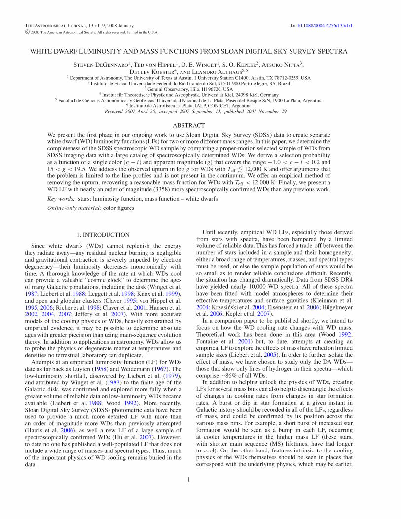
Figure 1. Plot of log g versus log Teff for the WDs in our sample. At temperaturesbelow ∼12,500 K, the log g values begin to rise to an extent unexplained bycurrent theory. The solid line is a function empirically fit to the real data. Thedashed line is the modest rise predicted by theory. The excess at a given Teff issubtracted from the measured log g value for some of our LFs.

(A color version of this figure is available in the online journal)

and associated errors. As their Figure 2 demonstrates, theyrecover a remarkably complete and uncontaminated sample ofthe candidate stars. They believe that they have recovered nearlyall of the DA WDs hotter than 10,000 K with SDSS spectra.

These stars form the core of our data sample. Eisensteinet al.’s final table lists data on 10,088 WDs. Of these, 7755are classified as single, nonmagnetic DA’s. Kepler et al. (2007)refit the spectra for these stars using the same autofit methodand Koester model atmospheres, but with a denser grid whichalso included models up to log g of 10.0. We use these newerfits in our analysis wherever they differ from Eisenstein et al.Of these 7755 entries, ∼600 are actually duplicate spectra ofthe same star. For our analysis, we take an average of the valuesderived from each individual spectrum weighted by the quotederrors. Our final sample contains 7128 single, nonmagnetic DAWDs.

As noted by Kleinman et al. (2004) and others, the surfacegravities determined from SDSS spectra show a suspiciousupturn below temperatures of about 12,000 K which increasesat cooler temperatures, as shown in our Figure 1.

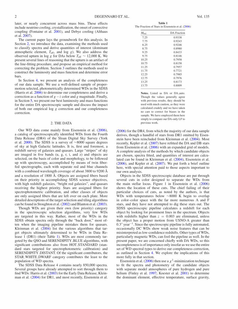
Figure 2. log g versus log Teff with the upturn in log g removed.

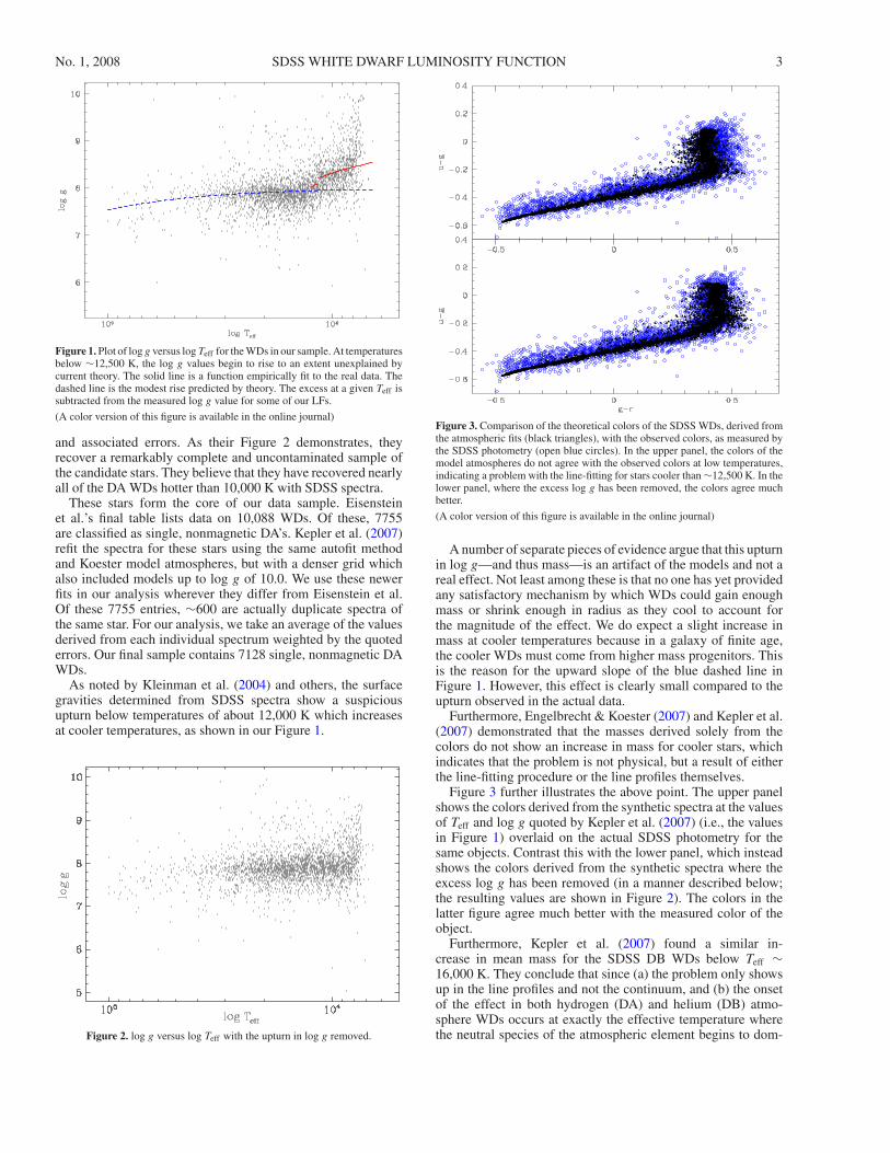
Figure 3. Comparison of the theoretical colors of the SDSS WDs, derived fromthe atmospheric fits (black triangles), with the observed colors, as measured bythe SDSS photometry (open blue circles). In the upper panel, the colors of themodel atmospheres do not agree with the observed colors at low temperatures,indicating a problem with the line-fitting for stars cooler than ∼12,500 K. In thelower panel, where the excess log g has been removed, the colors agree muchbetter.

(A color version of this figure is available in the online journal)

A number of separate pieces of evidence argue that this upturnin log g—and thus mass—is an artifact of the models and not areal effect. Not least among these is that no one has yet providedany satisfactory mechanism by which WDs could gain enoughmass or shrink enough in radius as they cool to account forthe magnitude of the effect. We do expect a slight increase inmass at cooler temperatures because in a galaxy of finite age,the cooler WDs must come from higher mass progenitors. Thisis the reason for the upward slope of the blue dashed line inFigure 1. However, this effect is clearly small compared to theupturn observed in the actual data.

Furthermore, Engelbrecht & Koester (2007) and Kepler et al.(2007) demonstrated that the masses derived solely from thecolors do not show an increase in mass for cooler stars, whichindicates that the problem is not physical, but a result of eitherthe line-fitting procedure or the line profiles themselves.

Figure 3 further illustrates the above point. The upper panelshows the colors derived from the synthetic spectra at the valuesof Teff and log g quoted by Kepler et al. (2007) (i.e., the valuesin Figure 1) overlaid on the actual SDSS photometry for thesame objects. Contrast this with the lower panel, which insteadshows the colors derived from the synthetic spectra where theexcess log g has been removed (in a manner described below;the resulting values are shown in Figure 2). The colors in thelatter figure agree much better with the measured color of theobject.

Furthermore, Kepler et al. (2007) found a similar in-crease in mean mass for the SDSS DB WDs below Teff ∼16,000 K. They conclude that since (a) the problem only showsup in the line profiles and not the continuum, and (b) the onsetof the effect in both hydrogen (DA) and helium (DB) atmo-sphere WDs occurs at exactly the effective temperature wherethe neutral species of the atmospheric element begins to dom-

4 DEGENNARO ET AL. Vol. 135

inate, the problem lies in the treatment of line broadening byneutral particles. This is supported further by the fact that as thespecies continues to become more neutral (i.e., as the tempera-ture drops), the problem grows worse.

However, more recent model calculations indicate that neu-tral broadening is not important in the DA WDs at temperaturesdown to at least 8500 K. Other possible mechanisms to explainthe observed upturn in log g include a flawed or incompletetreatment of convection, leading to errors in the temperaturestructure of the outer layers of the WD models, or the convec-tive mixing of helium from a lower layer in the atmosphere(Bergeron et al. 1990, 1995a). The latter would require a hydro-gen layer much thinner than any seismologically determined ina DA so far (Bradley 1998, 2001, 2006).

Until the problem with the model atmospheres is resolved,the best we can do is to empirically remove the log g upturn. Fora given Teff , we subtract the excess in the measured mean value(as fitted by the red solid lines in Figure 1) over the theoreticallyexpected mean (blue dashed line). Figure 2 shows the resultingvalues used. In fitting out the upturn this way, we make twoimplicit assumptions. First, we assume that the excess log g is afunction only of Teff ; if the problem is indeed due to the treatmentof neutral particles, we would expect only a small dependence onlog g. Second, we assume that the problem affects only the logg determination and not Teff . This latter assumption is unlikelyto be true, as the two parameters are correlated. In Section 5,we explore more fully the impact of this fitting procedure on theluminosity and mass functions.

3. CONSTRUCTING THE LUMINOSITY AND MASSFUNCTIONS

Since we are dealing with a magnitude-limited sample, themost luminous stars in our sample can be seen at much furtherdistances than the intrinsically fainter stars. We thus expect moreof them, proportionally, than we would in a purely volume-limited sample, and must make a correction for the differentobserving volumes. As shown by Wood & Oswalt (1998) andGeijo et al. (2006), the 1/Vmax method of Schmidt (1968)(described more fully in, e.g., Green (1980); Fleming et al.(1986)) provides an unbiased and reliable characterization ofthe WD LF.

In the 1/Vmax method, each star’s contribution to the totalspace density is weighted in inverse proportion to the totalvolume over which it would still be included in the magnitude-limited sample. Since the stars are not spherically distributed,but lie preferentially in the plane of the Galaxy, an additionalcorrection for the scale height of the Galactic disk must beincluded. For the purposes of comparison with previous work,we adopt a scale height of 250 pc.

To determine the absolute magnitude of each WD, we use theeffective temperatures and log g values provided by Kepler et al.(2007)—as corrected in Section 2—and fit each WD withan evolutionary model to determine the mass and radius. For7.0 < log g < 9.0, we use the mixed C/O models of Woodet al. (1995) and Fontaine et al. (2001), as calculated byBergeron et al. (1995b). For 9.0 < log g < 10.0, we use themodels of Althaus et al. (2005) with O/Ne cores, includingadditional sequences for masses larger than 1.3 M� calculatedspecifically for Kepler et al. (2007). Once we know the radius,we can calculate the absolute magnitude in each SDSS band byconvolving the synthetic WD atmospheres of Koester (Finleyet al. 1997; Koester et al. 2001) with the SDSS filter curves. We

apply bolometric corrections from Bergeron et al. (1995b) todetermine the bolometric magnitude. For the handful of stars(∼80–100) with log g values outside the range covered byBergeron’s tables, we use a simple linear extrapolation.

We then determine photometric distances to each star fromthe observed SDSS g magnitude. The SDSS, being concernedmostly with extragalactic objects, reports the total interstellarabsorption along each line of sight from the reddening maps ofSchlegel et al. (1998). Since the objects in our sample lie withinthe Galaxy, and most of them within a few hundred parsecs,they are affected by only a fraction of this reddening. FollowingHarris et al. (2006), we therefore assume that (1) objects within100 pc are not affected by reddening, (2) objects with Galacticheight |z| > 250 pc are reddened by the full amount, and(3) the reddening varies linearly between these two values. Thedistances and reddening are then fit iteratively from the observedand calculated absolute g magnitudes. In practice, the reddeningcorrection makes very little difference to the final LF (typicalAg values range from 0.01 to 0.05).

We calculate error bars on the LF using a Monte Carlosimulation, drawing random deviates in Teff , log g, and eachband of photometry from Gaussian distributions centered aroundthe measured value. The standard deviations in Teff and log g weuse for this scattering are 1.2 times the formal errors quoted inEisenstein et al. (2006) (their own analysis, based on repeatedautofit measurements on duplicate spectra of the same stars,suggests that the formal errors derived by their method are∼20% too small). The photometry errors come directly fromthe SDSS database. After scattering the parameters in this way,we recalculate the LF. We then add in quadrature the standarddeviation of each LF bin after 200 iterations and the countingerror for each bin (the errors for each individual star—taken tobe of the order of the star’s 1/Vmax statistical weight—summedin quadrature).

At an S/N of 16—the mean for the stars in our sample brighterthan g = 19.5—formal errors in Teff and log g are of order 1.5%.When propagated through our code, the mean errors in Mbol andmass are 0.35 dex and 9% (0.05 M�), respectively. For the starsbrighter than g = 19.0 used to compile our mass functionsthe average S/N is 19.5, leading to errors in Mbol and mass of0.35 dex and 7% (0.04 M�).

4. COMPLETENESS CORRECTIONS

The chief difficulty we have encountered in deriving ourLFs is unraveling the complicated way in which SDSS objectsare assigned spectral fibers. The SDSS is foremost a surveyof extragalactic objects and rarely targets WDs for follow-up spectroscopy explicitly. Most of the objects in our sampleare targeted by some other algorithm. In particular, there isconsiderable overlap in color between WDs and many QSOs.

A completeness correction could, in theory, be built from“first principles.” We know, for each object in the SDSSspectroscopic database, by which algorithm(s) it was targeted(or rejected) for spectroscopy, and by which algorithm it wasultimately assigned a fiber. And for each algorithm, we knowwhich objects were targeted, which were ultimately assigned afiber, and which, of the targeted objects, turned out to be WDs.However, the selection process is a multivariate function of fiveapparent magnitudes, and colors in spaces of as many as fourdimensions (which vary on the basis of the algorithm), as wellas the complex tiling algorithm. We believe such an undertakingto be unnecessary. Instead we have chosen to compare our

No. 1, 2008 SDSS WHITE DWARF LUMINOSITY FUNCTION 5

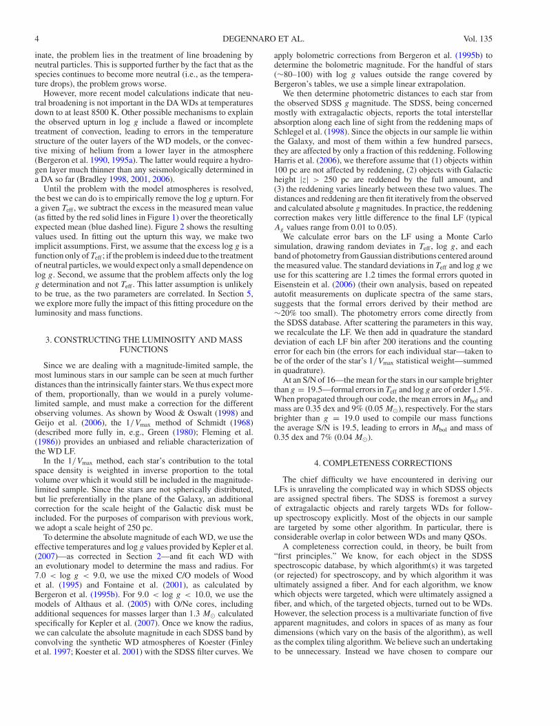
sample with the stars used to derive the WD LF of Harriset al. (2006). Given certain assumptions about completenessand contamination in both data sets, we derive a completenesscorrection as a function of a single color index (g − i) and gmagnitude.

The Harris et al. (2006) sample comes from photometricdata in the SDSS Data Release 3 (DR3). They selected objectsby using the reduced proper-motion diagram to separate WDsfrom more luminous subdwarfs of the same color. Briefly,they used color and proper motion (from USNO-B; Munnet al. 2004) to determine WD candidates from SDSS imagingdata. They then fitted candidates with WD model atmospherecolors to determine temperatures and absolute magnitudes,from which they derived photometric distances and—togetherwith proper motion—tangential velocities. In order to minimizecontamination, they adopted a tangential velocity cutoff of30 km s−1 and rejected all stars below this limit. The remaining6000 objects are, with a high and well-defined degree ofcertainty (∼98–99%), likely to be WDs.

If the database of SDSS spectra were complete, all of theseobjects would (eventually) have spectra, and all but 1–2%of contaminating objects would be confirmed to be WDs.Furthermore, all of the WDs that did not make it into theHarris et al. sample—because they were either missing from theMunn et al. (2004) proper-motion catalog, or had a tangentialvelocity below 30 km s−1—would also all have spectra. Insuch a perfect world, of course, no completeness correctionwould be necessary. However, since the SDSS does not obtaina spectrum of every object in its photometric database, asignificant percentage of the objects in Harris et al. will nothave spectra, or else will be dropped at some later point byEisenstein et al. and thus not make it into our spectroscopicsample. Our goal, then, is to look into all of the WDs in the Harriset al. sample that potentially could have made it into our sample,and determine which ones in fact did. If we assume that the WDsnot in Harris et al. follow the same distribution (an assumptionwe discuss more fully below), then we can take this as ameasure of the overall detection probability and invert it toget a completeness correction.

The imaging area of the DR3, from which Harris et al.derive their sample, is not the same as the spectroscopic areain the DR4. Therefore, for the purposes of this comparison, weremoved all stars not found in the area of sky common to the twodata sets from their respective samples. This left 5340 objectsclassified as WDs by Harris et al. that could potentially havebeen recovered by Eisenstein et al. Of these, 2572 were assignedspectral fibers in DR4, and 2346 were ultimately confirmed byEisenstein et al. to be WDs.

Since we wish to restrict our analysis to single (i.e.,nonbinary) DA WDs, we removed all stars classified asDA+M stars in either catalog. Unfortunately, given that theHarris catalog contains no further information as to the typeof WD, we were unable to remove the non-DA stars andsimply compare what remains with the Eisenstein sample.Instead, we compute the completeness for all of the WDs, underthe assumption—explored more fully below—that DA’s, as thelargest component of the WD population, dominate the selectionfunction.

Figure 4 shows a comparison of the two samples. The opensymbols are the complete Harris et al. sample (excluding those,as mentioned above, with Vtan < 30 km s−1, those not in theregion of sky covered by spectroscopy, and the DA+M stars).The gray squares lie outside the cuts in the color–color space

Figure 4. Color–color plot of the WDs in the two samples used to derive ourcompleteness correction. Open symbols are WDs from the Harris et al. (2006)sample that (a) were in the area of sky covered by spectroscopy in DR4, (b)had Vtan � 30 km s−1, and (c) were not determined by i- and z-band excessto be WD + main-sequence binaries. The filled circles are the stars for whichSDSS obtained spectra and Eisenstein et al. (2006) confirmed to be WDs.The dashed box shows a two-dimensional projection of the QSO targetingalgorithm’s exclusion region. The open gray squares are the WDs from Harriset al. that lie outside Eisenstein et al.’s color–color cuts. For clarity, only half ofthe points have been plotted.

imposed by Eisenstein et al. They may have spectra in SDSS, butthey were not fit by Eisenstein et al., and therefore will not havemade it into our sample. The filled green circles are the starsthat are in Eisenstein et al. In other words, if the SDSS spectralcoverage of WDs were complete, and Eisenstein et al. recoveredevery WD spectrum in SDSS, then all of the open circles wouldbe filled. The inside of the blue box is the exclusion regionfor the SDSS’s QSO targeting algorithm (Richards et al. 2002),specifically implemented to eliminate WDs from their sample.Note that our sample is more complete for the stars outside thisregion.

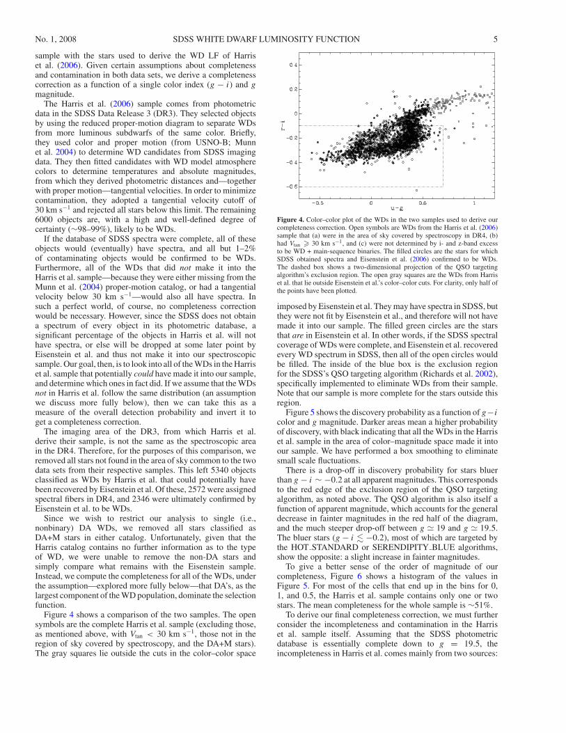
Figure 5 shows the discovery probability as a function of g−icolor and g magnitude. Darker areas mean a higher probabilityof discovery, with black indicating that all the WDs in the Harriset al. sample in the area of color–magnitude space made it intoour sample. We have performed a box smoothing to eliminatesmall scale fluctuations.

There is a drop-off in discovery probability for stars bluerthan g − i ∼ −0.2 at all apparent magnitudes. This correspondsto the red edge of the exclusion region of the QSO targetingalgorithm, as noted above. The QSO algorithm is also itself afunction of apparent magnitude, which accounts for the generaldecrease in fainter magnitudes in the red half of the diagram,and the much steeper drop-off between g � 19 and g � 19.5.The bluer stars (g − i � −0.2), most of which are targeted bythe HOT STANDARD or SERENDIPITY BLUE algorithms,show the opposite: a slight increase in fainter magnitudes.

To give a better sense of the order of magnitude of ourcompleteness, Figure 6 shows a histogram of the values inFigure 5. For most of the cells that end up in the bins for 0,1, and 0.5, the Harris et al. sample contains only one or twostars. The mean completeness for the whole sample is ∼51%.

To derive our final completeness correction, we must furtherconsider the incompleteness and contamination in the Harriset al. sample itself. Assuming that the SDSS photometricdatabase is essentially complete down to g = 19.5, theincompleteness in Harris et al. comes mainly from two sources:

6 DEGENNARO ET AL. Vol. 135

−1.0 −0.8 −0.6 −0.4 −0.2 0.0 0.2

1516

1718

19

g − i

g

Figure 5. Map of our completeness correction. Darker areas indicate more complete regions of the figure, with black being 100% complete. The overall completenessis of order ∼50%.

Figure 6. Histogram of the completeness values in Figure 5. Most of the 0, 1,and 0.5 values come from color–magnitude regions in which there are only oneor two stars in the Harris et al. sample available for comparison.

(1) the incompleteness in the Munn et al. (2004) propermotion catalog, and (2) the tangential velocity limit of 30 kms−1 imposed, which results in some low tangential velocityWDs being dropped from the sample. However, with onenegligible exception, none of the criteria used to target objectsfor spectroscopy in SDSS, nor those used by Eisenstein et al.to select WD candidates, depends explicitly on proper motionor tangential velocity. Thus we assume that the low-velocitystars—dropped from the Harris et al. sample—will be recoveredby Eisenstein et al. with the same probability as the high-velocitystars—i.e., the stars in Figure 4.

Contamination poses a somewhat more challenging problem.At first glance, it would seem that the reverse of the aboveprocess could be applied, whereby those objects in Harris etal. which did get spectral fibers—but were ultimately rejectedas WDs by Eisenstein et al.—could be removed from thesample, and those that did not get spectra could be assumed tofollow the same distribution. This latter assumption, however,is unlikely to be true. The SDSS gives very low priority totargeting WDs specifically, and we would thus expect a largerfraction of the objects that get spectral fibers to turn out to be

contaminating objects (in particular QSOs, of which we found13 in the Harris et al. sample) than if the fibers were assignedpurely randomly. Furthermore, many of the 225 objects thathave spectra in DR4 but are not included in the Eisensteinet al. catalog may actually be WDs which Eisenstein et al.’salgorithms dropped for some other reason, e.g., they lie outsidethe color and magnitude ranges used for initial candidateselection, or there is a problem (low S/N, bad pixels) with thespectrum. Approximately 100 appear to be DC WDs to whichthe SDSS spectroscopic pipeline assigned erroneous redhiftson the basis of weak noise features. Ultimately, we have chosento adopt the contamination fraction of Harris et al. (2%) forthe whole sample, and have reduced our final completenesscorrection accordingly. This choice has a negligible effect on thesmall scale structure of the WD LF in which we are interested.

Finally, we note that the Harris et al. sample has an apparentmagnitude limit of g = 19.5, whereas the spectroscopic sam-ple contains objects down to g � 20.5. Given that the SDSStargeting algorithms are themselves functions of apparent mag-nitude, our completeness correction is as well. An extrapolationof our discovery probability is problematic in this area, though,because this is exactly the apparent magnitude where the QSOtargeting algorithm drops off rapidly. We have decided to imposea magnitude cutoff of g = 19.5 in our sample. This reduces oursample by nearly half, with a corresponding increase in countingerror. However, since SDSS spectra have a small range of ex-posure times (45–60 min), fainter apparent magnitude usuallytranslates directly into lower S/N and larger errors in derivedparameters.

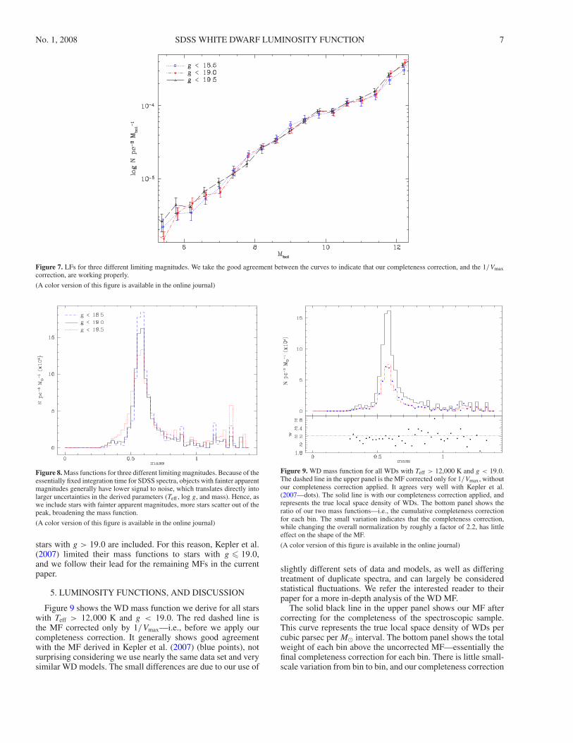
Figure 7 shows the LFs we derive for different choices oflimiting magnitude. We take the generally good agreementbetween the curves to indicate that our completeness correctionis doing its job correctly in the g magnitude direction.

Figure 8 similarly shows the mass functions (MFs) we derivefor different choices of limiting magnitude. In the case of theMF, the S/N of the spectra becomes a much bigger factor.As a consequence of the essentially constant exposure timesof SDSS spectra, the parameters (Teff and log g) determinedfrom the spectra of fainter objects have larger errors, whichcauses a larger error in mass. Thus, the MF is broadened when

No. 1, 2008 SDSS WHITE DWARF LUMINOSITY FUNCTION 7

Figure 7. LFs for three different limiting magnitudes. We take the good agreement between the curves to indicate that our completeness correction, and the 1/Vmaxcorrection, are working properly.

(A color version of this figure is available in the online journal)

Figure 8. Mass functions for three different limiting magnitudes. Because of theessentially fixed integration time for SDSS spectra, objects with fainter apparentmagnitudes generally have lower signal to noise, which translates directly intolarger uncertainties in the derived parameters (Teff , log g, and mass). Hence, aswe include stars with fainter apparent magnitudes, more stars scatter out of thepeak, broadening the mass function.

(A color version of this figure is available in the online journal)

stars with g > 19.0 are included. For this reason, Kepler et al.(2007) limited their mass functions to stars with g � 19.0,and we follow their lead for the remaining MFs in the currentpaper.

5. LUMINOSITY FUNCTIONS, AND DISCUSSION

Figure 9 shows the WD mass function we derive for all starswith Teff > 12,000 K and g < 19.0. The red dashed line isthe MF corrected only by 1/Vmax—i.e., before we apply ourcompleteness correction. It generally shows good agreementwith the MF derived in Kepler et al. (2007) (blue points), notsurprising considering we use nearly the same data set and verysimilar WD models. The small differences are due to our use of

Figure 9. WD mass function for all WDs with Teff > 12,000 K and g < 19.0.The dashed line in the upper panel is the MF corrected only for 1/Vmax, withoutour completeness correction applied. It agrees very well with Kepler et al.(2007—dots). The solid line is with our completeness correction applied, andrepresents the true local space density of WDs. The bottom panel shows theratio of our two mass functions—i.e., the cumulative completeness correctionfor each bin. The small variation indicates that the completeness correction,while changing the overall normalization by roughly a factor of 2.2, has littleeffect on the shape of the MF.

(A color version of this figure is available in the online journal)

slightly different sets of data and models, as well as differingtreatment of duplicate spectra, and can largely be consideredstatistical fluctuations. We refer the interested reader to theirpaper for a more in-depth analysis of the WD MF.

The solid black line in the upper panel shows our MF aftercorrecting for the completeness of the spectroscopic sample.This curve represents the true local space density of WDs percubic parsec per M� interval. The bottom panel shows the totalweight of each bin above the uncorrected MF—essentially thefinal completeness correction for each bin. There is little small-scale variation from bin to bin, and our completeness correction

8 DEGENNARO ET AL. Vol. 135

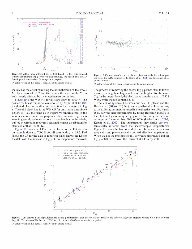
Figure 10. WD MFs for WDs with Teff > 8000 K and g < 19.0 both with andwithout the upturn in log g for cooler stars removed. The solid line is the MFfrom Figure 9 renormalized for comparison purposes.

(A color version of this figure is available in the online journal)

mainly has the effect of raising the normalization of the wholeMF by a factor of ∼2.2. In other words, the shape of the MF isnot strongly affected by the completeness correction.

Figure 10 is the WD MF for all stars down to 8000 K. Thedashed red line is for the data as reported by Kepler et al. (2007),the dotted blue line is after our correction for the upturn in logg. The solid black line is the WD MF for only those stars above12,000 K (i.e., the same as in Figure 9) renormalized to thesame scale for comparison purposes. There are more high massstars in general, and one spuriously large bin, but on the whole,our log g correction recovers a reasonable mass distribution forstars cooler than 12,000 K.

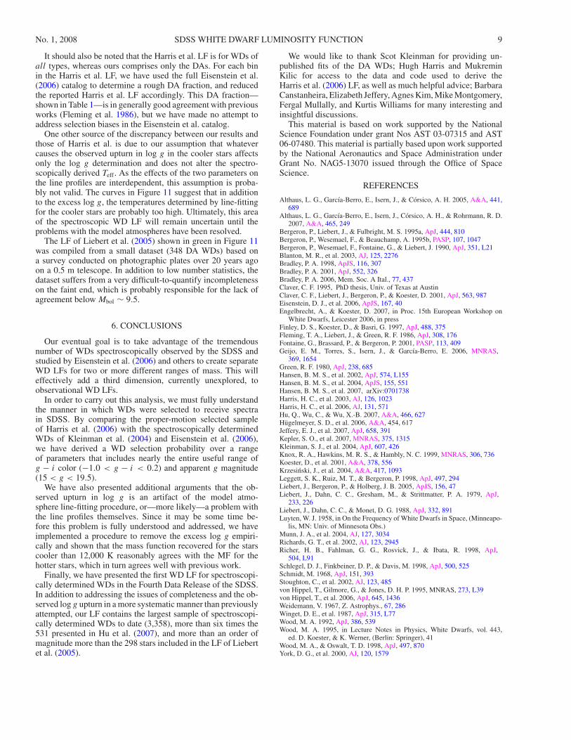
Figure 11 shows the LF we derive for all of the DA stars inour sample down to 7000 K for all stars with g < 19.5. Redshows the LF for the data as reported; black shows the LF forthe data with the increase in log g at low temperature removed.

Figure 12. Comparison of the spectrally and photometrically derived temper-atures for the WDs common to the Harris et al. (2006) and Eisenstein et al.(2006) samples.

(A color version of this figure is available in the online journal)

The process of removing the excess log g pushes stars to lowermasses, making them larger and therefore brighter for the sameTeff . In the range plotted, the black curve contains a total of 3358WDs, while the red contains 2940.

The lack of agreement between our best LF (black) and theHarris et al. (2006) LF (blue) can be attributed, at least in part,to the differing assumptions used in creating the two LFs. Harriset al. derived their temperatures by fitting Bergeron models tothe photometry assuming a log g of 8.0 for every star, a poorassumption for more than 30% of WDs (Liebert et al. 2005;Kepler et al. 2007). The temperatures they derive are sys-tematically different from the spectroscopic temperatures;Figure 12 shows the fractional difference between the spectro-scopically and photometrically derived effective temperatures.When we use the photometrically derived temperatures and setlog g = 8.0, we recover the Harris et al. LF fairly well.

Figure 11. LFs derived in this paper. Removing the log g upturn makes each affected star less massive, and therefore larger and brighter, pushing it to a more leftwardMbol bin. The results of Harris et al. (2006) and Liebert et al. (2005) are shown for comparison.

(A color version of this figure is available in the online journal)

No. 1, 2008 SDSS WHITE DWARF LUMINOSITY FUNCTION 9

It should also be noted that the Harris et al. LF is for WDs ofall types, whereas ours comprises only the DAs. For each binin the Harris et al. LF, we have used the full Eisenstein et al.(2006) catalog to determine a rough DA fraction, and reducedthe reported Harris et al. LF accordingly. This DA fraction—shown in Table 1—is in generally good agreement with previousworks (Fleming et al. 1986), but we have made no attempt toaddress selection biases in the Eisenstein et al. catalog.

One other source of the discrepancy between our results andthose of Harris et al. is due to our assumption that whatevercauses the observed upturn in log g in the cooler stars affectsonly the log g determination and does not alter the spectro-scopically derived Teff . As the effects of the two parameters onthe line profiles are interdependent, this assumption is proba-bly not valid. The curves in Figure 11 suggest that in additionto the excess log g, the temperatures determined by line-fittingfor the cooler stars are probably too high. Ultimately, this areaof the spectroscopic WD LF will remain uncertain until theproblems with the model atmospheres have been resolved.

The LF of Liebert et al. (2005) shown in green in Figure 11was compiled from a small dataset (348 DA WDs) based ona survey conducted on photographic plates over 20 years agoon a 0.5 m telescope. In addition to low number statistics, thedataset suffers from a very difficult-to-quantify incompletenesson the faint end, which is probably responsible for the lack ofagreement below Mbol ∼ 9.5.

6. CONCLUSIONS

Our eventual goal is to take advantage of the tremendousnumber of WDs spectroscopically observed by the SDSS andstudied by Eisenstein et al. (2006) and others to create separateWD LFs for two or more different ranges of mass. This willeffectively add a third dimension, currently unexplored, toobservational WD LFs.

In order to carry out this analysis, we must fully understandthe manner in which WDs were selected to receive spectrain SDSS. By comparing the proper-motion selected sampleof Harris et al. (2006) with the spectroscopically determinedWDs of Kleinman et al. (2004) and Eisenstein et al. (2006),we have derived a WD selection probability over a rangeof parameters that includes nearly the entire useful range ofg − i color (−1.0 < g − i < 0.2) and apparent g magnitude(15 < g < 19.5).

We have also presented additional arguments that the ob-served upturn in log g is an artifact of the model atmo-sphere line-fitting procedure, or—more likely—a problem withthe line profiles themselves. Since it may be some time be-fore this problem is fully understood and addressed, we haveimplemented a procedure to remove the excess log g empiri-cally and shown that the mass function recovered for the starscooler than 12,000 K reasonably agrees with the MF for thehotter stars, which in turn agrees well with previous work.

Finally, we have presented the first WD LF for spectroscopi-cally determined WDs in the Fourth Data Release of the SDSS.In addition to addressing the issues of completeness and the ob-served log g upturn in a more systematic manner than previouslyattempted, our LF contains the largest sample of spectroscopi-cally determined WDs to date (3,358), more than six times the531 presented in Hu et al. (2007), and more than an order ofmagnitude more than the 298 stars included in the LF of Liebertet al. (2005).

We would like to thank Scot Kleinman for providing un-published fits of the DA WDs; Hugh Harris and MukreminKilic for access to the data and code used to derive theHarris et al. (2006) LF, as well as much helpful advice; BarbaraCanstanheira, Elizabeth Jeffery, Agnes Kim, Mike Montgomery,Fergal Mullally, and Kurtis Williams for many interesting andinsightful discussions.

This material is based on work supported by the NationalScience Foundation under grant Nos AST 03-07315 and AST06-07480. This material is partially based upon work supportedby the National Aeronautics and Space Administration underGrant No. NAG5-13070 issued through the Office of SpaceScience.

REFERENCES

Althaus, L. G., Garcıa-Berro, E., Isern, J., & Corsico, A. H. 2005, A&A, 441,689

Althaus, L. G., Garcıa-Berro, E., Isern, J., Corsico, A. H., & Rohrmann, R. D.2007, A&A, 465, 249

Bergeron, P., Liebert, J., & Fulbright, M. S. 1995a, ApJ, 444, 810Bergeron, P., Wesemael, F., & Beauchamp, A. 1995b, PASP, 107, 1047Bergeron, P., Wesemael, F., Fontaine, G., & Liebert, J. 1990, ApJ, 351, L21Blanton, M. R., et al. 2003, AJ, 125, 2276Bradley, P. A. 1998, ApJS, 116, 307Bradley, P. A. 2001, ApJ, 552, 326Bradley, P. A. 2006, Mem. Soc. A Ital., 77, 437Claver, C. F. 1995, PhD thesis, Univ. of Texas at AustinClaver, C. F., Liebert, J., Bergeron, P., & Koester, D. 2001, ApJ, 563, 987Eisenstein, D. J., et al. 2006, ApJS, 167, 40Engelbrecht, A., & Koester, D. 2007, in Proc. 15th European Workshop on

White Dwarfs, Leicester 2006, in pressFinley, D. S., Koester, D., & Basri, G. 1997, ApJ, 488, 375Fleming, T. A., Liebert, J., & Green, R. F. 1986, ApJ, 308, 176Fontaine, G., Brassard, P., & Bergeron, P. 2001, PASP, 113, 409Geijo, E. M., Torres, S., Isern, J., & Garcıa-Berro, E. 2006, MNRAS,

369, 1654Green, R. F. 1980, ApJ, 238, 685Hansen, B. M. S., et al. 2002, ApJ, 574, L155Hansen, B. M. S., et al. 2004, ApJS, 155, 551Hansen, B. M. S., et al. 2007, arXiv:0701738Harris, H. C., et al. 2003, AJ, 126, 1023Harris, H. C., et al. 2006, AJ, 131, 571Hu, Q., Wu, C., & Wu, X.-B. 2007, A&A, 466, 627Hugelmeyer, S. D., et al. 2006, A&A, 454, 617Jeffery, E. J., et al. 2007, ApJ, 658, 391Kepler, S. O., et al. 2007, MNRAS, 375, 1315Kleinman, S. J., et al. 2004, ApJ, 607, 426Knox, R. A., Hawkins, M. R. S., & Hambly, N. C. 1999, MNRAS, 306, 736Koester, D., et al. 2001, A&A, 378, 556Krzesinski, J., et al. 2004, A&A, 417, 1093Leggett, S. K., Ruiz, M. T., & Bergeron, P. 1998, ApJ, 497, 294Liebert, J., Bergeron, P., & Holberg, J. B. 2005, ApJS, 156, 47Liebert, J., Dahn, C. C., Gresham, M., & Strittmatter, P. A. 1979, ApJ,

233, 226Liebert, J., Dahn, C. C., & Monet, D. G. 1988, ApJ, 332, 891Luyten, W. J. 1958, in On the Frequency of White Dwarfs in Space, (Minneapo-

lis, MN: Univ. of Minnesota Obs.)Munn, J. A., et al. 2004, AJ, 127, 3034Richards, G. T., et al. 2002, AJ, 123, 2945Richer, H. B., Fahlman, G. G., Rosvick, J., & Ibata, R. 1998, ApJ,

504, L91Schlegel, D. J., Finkbeiner, D. P., & Davis, M. 1998, ApJ, 500, 525Schmidt, M. 1968, ApJ, 151, 393Stoughton, C., et al. 2002, AJ, 123, 485von Hippel, T., Gilmore, G., & Jones, D. H. P. 1995, MNRAS, 273, L39von Hippel, T., et al. 2006, ApJ, 645, 1436Weidemann, V. 1967, Z. Astrophys., 67, 286Winget, D. E., et al. 1987, ApJ, 315, L77Wood, M. A. 1992, ApJ, 386, 539Wood, M. A. 1995, in Lecture Notes in Physics, White Dwarfs, vol. 443,

ed. D. Koester, & K. Werner, (Berlin: Springer), 41Wood, M. A., & Oswalt, T. D. 1998, ApJ, 497, 870York, D. G., et al. 2000, AJ, 120, 1579