SERC DISCUSSION PAPER 71

Where is the Economics in SpatialEconometrics?Luisa Corrado (Faculty of Economics, University of Cambridge,International Economics , University of Rome Tor Vergata)Bernard Fingleton (SERC, SIRE, University of Strathclyde)

March 2011

This work is part of the research programme of the independent UK Spatial Economics Research Centre funded by the Economic and Social Research Council (ESRC), Department for Business, Innovation and Skills (BIS), the Department for Communities and Local Government (CLG), and the Welsh Assembly Government. The support of the funders is acknowledged. The views expressed are those of the authors and do not represent the views of the funders. © L. Corrado and B. Fingleton, submitted 2011

Where is the Economics in Spatial Econometrics?

Luisa Corrado* and Bernard Fingleton**

March 2011 * Faculty of Economics, University of Cambridge, International Economics, University of Rome Tor Vergata ** SERC, SIRE, University of Strathclyde

Abstract Spatial econometrics has been criticized by some economists because some model specifications have been driven by data-analytic considerations rather than having a firm foundation in economic theory. In particular this applies to the so-called W matrix, which is integral to the structure of endogenous and exogenous spatial lags, and to spatial error processes, and which are almost the sine qua non of spatial econometrics. Moreover it has been suggested that the significance of a spatially lagged dependent variable involving W may be misleading, since it may be simply picking up the effects of omitted spatially dependent variables, incorrectly suggesting the existence of a spillover mechanism. In this paper we review the theoretical and empirical rationale for network dependence and spatial externalities as embodied in spatially lagged variables, arguing that failing to acknowledge their presence at least leads to biased inference, can be a cause of inconsistent estimation, and leads to an incorrect understanding of true causal processes. Keywords: Spatial econometrics, endogenous spatial lag, exogenous spatial lag, spatially dependent errors, network dependence, externalities, the W matrix, panel data with spatial effects, multilevel models with spatial effects JEL Classifications: C21, C31, R0

1 INTRODUCTION

The critique of spatial econometrics emanating from some economists is, we assert at the outset,based on imprecise and ill-informed perceptions of the sophistication and diversity of the work ofthe spatial econometrics and wider academic community. The argument is that standard spatialeconometrics is typically applied in a mechanical fashion, variables are introduced simply becausethey are signi�cant, without a priori rationale, spatial econometricians often work in isolation fromurban economists and other regional scientists, and overall there is a lack of theoretical justi�cationfor variables that characterize spatial econometric models.1 An engagement with the literature showsthis to be a misrepresentation. There are numerous examples of single equation cross-sectional spatialeconometric models, multiequation speci�cations, and panel models incorporating spatial e¤ects, inwhich economic theory is fundamental to the speci�cation of the reduced form, including speci�cationsbased on neoclassical growth theory (Ertur and Koch (2007), Fingleton and Lopez-Bazo (2006)),urban economics (Fingleton (2006), Barde (2010)) and on the wage equation from new economicgeography (Fingleton (2003)). Almost invariably these speci�cations are elaborations of mainstreamtheory incorporating externalities in the form of spatial spillovers, being characterized by the presenceof the trademark component of the spatial econometric model, namely the spatial lag, which can beconsidered to be the sine qua non of spatial econometrics. While the theory underlying these modelsis often exceptionally well established and well received, nevertheless it is also true that there are casesin which spatial econometric work has been too casual in its attempt to base model speci�cations oneconomic theory. Our �rst main contribution is to highlight this criticism. Often there is no attempt tomake theory testing a focal point of the research, and too often we see an emphasis on diagnostics andempirical model validity as the most important criteria to be used to signify a good model, without anyattempt to relate to real or theorized economic processes and mechanisms. Most signi�cantly, when itcomes to the spatial lag, which is based on the so-calledW matrix of spatial weights, many economistsare skeptical, puzzled, or both. The values in the cells of W comprise an explicit hypothesis aboutthe strength of inter-location connection (typically towns, regions, or countries), and in many casesthe matrix product ofW and endogenous variable Y; namely the endogenous spatial lagWY, oftenproves to be a highly signi�cant variable. It has been suggested by the skeptics that the signi�cance ofexplanatory variableWY may be misleading, since it may be simply picking up the e¤ects of omittedspatially dependent variables,WX, incorrectly suggesting the existence of a spillover mechanism.

One way out of the W matrix conundrum may appear to be via hierarchical modelling, whichhas had only very limited exposure in the spatial economics literature (exceptions being Smith andLeSage (2004), Parent and LeSage (2008)). Hierarchical models (also known as multilevel models) arebecoming increasingly popular across the range of the social sciences, as researchers come to appreciatethat observed outcomes depend on variables organized in a nested hierarchy.2 In regional science andspatial economics, we can often envisage a hierarchy of e¤ects from cities, regions containing cities, andcountries containing regions. Failure to recognize these e¤ects emanating from di¤erent hierarchicallevels can lead to incorrect inference. The second major contribution of this paper is to point this outand to show that something equivalent toW is very much a cognate part of a hierarchical approach,with an enhancement to hierarchical modelling coming by way of incorporating spatial e¤ects viaW.

1The paper by Pinkse and Slade (2010) raises some additional di¢ cult-to-resolve problems arising from a limited andsomewhat atypical selection of the so-called �spatial econometrics�literature.

2Over the past decade there has been a development of methods which have enabled researchers to model hierarchicaldata. Examples of these methods include multilevel models (see, for example, Goldstein (1998)), random coe¢ cientmodels (Longford (1993)) and hierarchical multilevel models proposed by Goldstein (1986) based on iterative generalizedleast squares (IGLS).

2

We demonstrate that the inclusion of interdependence between groups in the form of spatial e¤ects,WX; has two main advantages: (i) it avoids the omitted variable problem that may a­ ict modelswith endogenous spatial lags and (ii) it introduces a source of exogenous variation that allows theidenti�cation of both endogenous and exogenous group e¤ects.

2 W WITHIN SPATIAL ECONOMETRIC SPECIFICATIONS

The square matrixW is of dimension N , where N is the number of nodes in a network, with the valuein typical cellWjh quantifying the hypothesized strength of interaction between nodes j and h. Here westress that nodes need not necessarily be places in order to draw on the wider literature that providesadditional support to the concept of network interaction. Typically all of the diagonal elements ofWare zero, and I��W is non-singular. Also, following Kapoor, Kelejian, and Prucha (2007) and Kelejianand Prucha (1998),W should be uniformly bounded in absolute value, meaning that a constant c existssuch that max1�j�N

PNh=1 j Wjh j� c � 1 and max1�j�N

PNh=1 j Wjh j� c � 1 so as to produce

asymptotic results required for consistent estimation.In a single equation context, multiplying W by a N� 1 vector (dependent variable) Y, gives

the endogenous spatial lag WY, which is an integral component of numerous spatial econometricmodels. However given the N � k matrix of variables X, additional spatially lagged variables canbe introduced, forming the columns of the matrixWX. Also we can add a hypothesis that the errorsmay be spatially dependent. Following Anselin, Le Gallo, and Jayet (2007), who write from a spatialpanel data perspective, there are four ways we might wish to model spatial e¤ects operating throughthe error term, namely i) direct representation, which originates from the geostatistical literature(Cressie (2003)); as noted by Anselin (2003), this requires exact speci�cation of a smooth decay withdistance and a parameter space commensurate with a positive de�nite error variance-covariance matrix.Alternatively, as in Conley (1999), a looser de�nition of the distance decay may be implemented,leading to non-parametric estimation; ii) spatial error processes typi�ed by much work in spatialeconometrics (Anselin (1988)), based on a matrix, say M, which is N �N with similar properties toW and which may or may not be the same asW; de�ning indirectly the spatial structure of the non-zero elements of the error variance-covariance matrix. LikeW, theM matrix comprises non-negativevalues representing the a priori assumption about interaction strength between location pairs de�nedby speci�c rows and columns of M, normally with zeros on the main diagonal. iii) common factormodels originating from the time series literature (Hsiao and Pesaran (2008), Pesaran (2007), andKapetanios and Pesaran (2005)) and iv) spatial error components models (Kelejian and Robinson(1995), Anselin and Moreno (2003)), which we consider subsequently.

Allowing endogenous and exogenous spatial lags, plus a spatial error process, and assuming nodesare linked by network dependence matrixW for the lags and byM for the error process, and assum-ing autoregressive processes, the typical single equation spatial econometric model speci�cation, theSARAR(1,1) model, is

Y = �WY +X� +WX�x + " (1)

" = �M"+ � (2)

� � iid(0; �2I) (3)

In (1), � is a scalar coe¢ cient, � and �x are k � 1 vectors of coe¢ cients, and " is an N � 1 vector

3

of disturbances. For the error process, we have the scalar � and the N �1 vector of innovations �drawn from an iid distribution with variance �2:

We extend the scope of the spatial econometric models in two ways, �rst by introducing the timedimension, thus allowing panel data models with network dependence, and secondly by consideringmultilevel models (see Corrado and Fingleton (2010)).

Consider a simple random e¤ects panel speci�cation for time t = 1; :::; T and for individual i =1; :::; N given by:

Yit = �0t + �1Xit + �it (4)

�0t = �0 + �i

with �it � iid(0; �2�) and �i � iid(0; �2�) which can be rewritten as:

Yit = �0 + �1Xit + �i + �it (5)

where Yit is individual i�s response at time t; Xit is the exogenous variable, �i is an error speci�c toeach individual and �it is a transient error component speci�c to each time and each individual. Wecan introduce spatial e¤ects both as an endogenous spatial lag:

Yit = �0 + �WYit + �1Xit + �i + �it (6)

and as an autoregressive error process:

Yit = �0 + �WYit + �1Xit + eit (7)

eit = �Meit + �it

and generalizing to k regressors in the panel context this becomes:

Y = �(IT W)Y +X� + e (8)

in which Y is a TN � 1 vector of observations obtained by stacking Yit for i = 1:::N and t = 1 : : : T ,X is a TN � k matrix of regressors and � is a k � 1 vector of coe¢ cients.

In addition, given a TN � TN identity matrix with 1s, the NT � 1 vector e is

e = (INT � �IT M)�1� (9)

in which � is an NT � 1 vector of innovations, � is a scalar parameter and M is an N � N matrixwith similar properties to W. Regarding the error components in space-time, time dependency isintroduced into the innovations via the permanent individual error component �, thus:

� � iid(0; �2�) (10)

� � iid(0; �2�) (11)

� = (�T IN )�+ � (12)

4

so that � is an N � 1 vector of random e¤ects speci�c to each individual, � is the transient errorcomponent comprising an NT � 1 vector of errors speci�c to each individual and time, �T is a T � 1matrix with 1s , and �T IN is a TN � N matrix equal to T stacked matrices. The result is thatthe TN � TN innovations variance-covariance matrix � is nonspherical. Also �21 = �

2� + T�

2�: Note

that this di¤ers from the speci�cations given by Anselin (1988) and by Baltagi and Li (2006), wherethe autoregressive error process is con�ned to �: In contrast the Kapoor, Kelejian, and Prucha (2007)set-up assumes that the individual e¤ects � have the same autoregressive process.

3 PUTTING SOME ECONOMICS INTO W

The suggestion that spatial econometrics may have been somewhat �mechanical�in its application isundoubtedly true in instances where little care has been taken regarding the theoretical basis of themodel speci�cation. In this section we seek to show that in many applications of spatial econometrics,considerable attention has been given to specifying the matricesW andM in a rational manner thatattempts to represent as far as possible real social and economic processes. Hence we argue that inmany cases the presence of a spatial lag, sayWY, is necessary because it does re�ect a true interactionand is not simply a surrogate for some omitted variables. In fact, it appears that an absence of detailedconsideration for the structure ofW; or indeed rejection of an approach based onW, has come fromanalysts who are not particularly interested in the spatial processes per se, but see spatial dependenceas a something of a nuisance which, yes, has to be allowed for in modelling but which is not the focalpoint of their research. In this case spatial error dependence can be treated in very general terms, sayby Spatial Heteroscedastic Autocorrelation Consistent estimation or by common factor approaches.

We �rst focus on the very basic form ofW matrix, which has close links with time series analysis.In fact, it is easy to show that an autoregressive process in time has an equivalent to theW matrix,as demonstrated in Fingleton (2009).

Consider the W� matrix , in which W �jh = 1 if location pair i and j are close to each other in

space, and W �jh = 0 otherwise. By close, we typically mean contiguous. For time series we have a

comparable contiguity matrix, let us call it H. To see the near equivalence of H andW�, consider adata generating process for T periods,

Y (t) = �Y (t� 1) + "(t) (13)

"(1) = Y (1) = 0

� < 1; " � N(0; �2); t = 2; :::; T

This generates a stationary time series. In matrix terms an entirely equivalent data generatingprocess is given by

Y = �HY + " (14)

in which Y is a T � 1 vector, � is a scalar parameter, " is a T � 1 vector of disturbances and H is a T� T matrix with row t designating the same time point as column t and 1s indicating time proximity.In spatial series,W� is N � N , where N is the number of places or nodes on the network. Below weshow a typicalW� matrix for N = 10, and its time series counterpart H.

5

H =

266666666666666664

0 0 0 0 0 0 0 0 0 0

1 0 0 0 0 0 0 0 0 0

0 1 0 0 0 0 0 0 0 0

0 0 1 0 0 0 0 0 0 0

0 0 0 1 0 0 0 0 0 0

0 0 0 0 1 0 0 0 0 0

0 0 0 0 0 1 0 0 0 0

0 0 0 0 0 0 1 0 0 0

0 0 0 0 0 0 0 1 0 0

0 0 0 0 0 0 0 0 1 0

377777777777777775W� =

266666666666666664

0 0 0 1 0 0 0 0 0 0

0 0 0 1 1 0 0 0 0 0

0 0 0 0 1 1 0 0 0 0

1 1 0 0 0 0 0 0 0 0

0 1 1 0 0 0 0 0 1 1

0 0 1 0 0 0 0 1 0 1

0 0 0 0 0 0 0 0 1 0

0 0 0 0 0 1 0 0 0 1

0 0 0 0 1 0 1 0 0 1

0 0 0 0 1 1 0 1 1 0

377777777777777775Figures 1-3 show small hypothetical networks which can be represented as simple binary-valued

W� matrices.

W�A =

26666666666664

0 1 1 1 1 1 1 1

1 0 0 0 0 0 0 0

1 0 0 0 0 0 0 0

1 0 0 0 0 0 0 0

1 0 0 0 0 0 0 0

1 0 0 0 0 0 0 0

1 0 0 0 0 0 0 0

1 0 0 0 0 0 0 0

37777777777775W�

B =

266666664

0 1 1 1 1 1

1 0 1 1 1 1

1 1 0 1 1 1

1 1 1 0 1 1

1 1 1 1 0 1

1 1 1 1 1 1

377777775W�

C =

266666664

0 1 0 0 0 0

1 0 1 0 0 1

0 1 0 1 0 0

0 0 1 0 0 0

0 0 0 0 0 1

0 1 0 0 1 0

377777775

Typically in practice one would scale the matrix W�, say by the maximum eigenvalue, since thisclearly indicates �allowable�values that avoid singularities. One way to do this is by

W =W�

max(eig)(15)

in which max(eig) denotes the maximum eigenvalue of W�, where W� is such that real eigenvaluescan be obtained. Using this normalization, the maximum eigenvalue of W is 1, and the continuousrange for � in which (I � �W) is non-singular is 1

min(eig) < � < 1. An alternative to this, due to Ord(1975), is

W = D�0:5W�D�0:5 (16)

in which the diagonal matrix D takes values equal to the row sums ofW�: Most applications in spatialeconometrics scale the individual rows (or columns) ofW� by the row totals, so that theW rows sumto 1. In both these alternatives the same conditions apply for non-singularity. WithW thus de�ned,the spatial data generating process is

Y = �WY + " (17)

which is identical to the time series data generating process, except thatW replaces H and � replaces�. As � ! 1; we approach near unit root spatial autoregressive processes, with similar consequencesas in non-stationary time series.

6

Figure 1: Star (A)

Figure 2: Complete Network (B)

F

B

E

D

A

C

Figure 3: Nearest Neighbor (C)

7

While we have given some emphasis to the similarity of the DGP for autoregressive time series andspatial series, there are major dissimilarities on account of the multilateral nature of spatial interaction.In contrast, with time there are only two directions, forward and backwards. One of the contributionsof Cli¤ and Ord (1973, 1981) was to extend the de�nition of the matrix W to accommodate thedistinctiveness of spatial processes. Spillovers have diverse origins, and therefore one would anticipatethat the way to model them takes on various forms. For instance, they may be the outcome of networkeconomics Goyal (2009), commuting,3 migration, displaced demand and supply e¤ects in the housingmarket, input-output linkages, competition and coordination between �rms, localized information�ows through social networks, strategic interaction between policy makers,4 tax competition betweenlocal authorities, or even simply arbitrary boundaries causing spatial autocorrelation. We cannot dealwith all of these cases, so in the following paragraphs we focus on a selection, commencing with thetraditional distance-based unidimensional measures adopted in spatial econometrics (Anselin (1988))and introduce other multidimensional measures based on various notions of social or economic distance.Typically, isotropy is assumed, so that only distance between j and h is relevant, not the directionj to h. These may provide the basis for direct or indirect estimation of the error variance-covariancematrix, including the spillover in error components models.

Moving beyond crude measures of between-group spatial �distance�, such as the simple notionsof proximity and contiguity, leads us to slightly more elaborate speci�cations which nonetheless arestill based on the physical features of geographical units. For example Cli¤ and Ord (1973) combinedistance and length of the common border between contiguous spatial units thus:

Wjh = (djh)a ��jh�b (18)

where djh denotes the distance between locations j and h and �jh is the proportion of the boundary ofj shared with h whereas a and b are parameters. More general distance measures include multidimen-sional indicator functions. For example, Bodson and Peters (1975) use a general accessibility weight(calibrated between 0 and 1) which combines in a logistic function several channels of communicationbetween regions such as railways, motorways etc.:

Wjh =

JXj=1

pj (a=1 + b exp(�cjdjh)) (19)

where pj indicates the relative importance of the means of communication j: The sum is over the Jmeans of communication with djh equal to the distance from j to h; a; b and cj are parameters whichneed to be estimated.

The above measures are less useful when the spatial interaction is determined by purely economicvariables which may have little to do with spatial con�guration of boundaries or geographical distanceper se. This introduces the notion of economic distance, and developments in the conceptualization ofeconomic distance have been surveyed in Greenhut, Norman, and Hung (1987). According to Fingletonand Le Gallo (2008) �the spillover between areas will not simply be a function of spatial propinquity,to the exclusion of other e¤ects�and �it is more realistic to base it on relative �economic distance�.Big towns and cities are less remote than their geographical separation would imply, whereas verysmall locations are often isolated from one another�. Hence economic distance re�ects the reduced

3For example, Holly, Pesaran, and Yamagata (2010) suggest a weighting matrix in a house price equation whereconnections between London and other UK regions are based on the in�ow and out�ow of commuters.

4Bhattacharjee and Holly (2006) �nd evidence of strategic spillovers across the members of the Bank of England�sMonetary Policy Committee in the way they vote on interest rate changes.

8

transaction costs associated with �ows between geographically remote cities, which have better com-munications infrastructure, lower costs of information gathering and uncertainty, and similar economicand employment structures. Economic distance features in the work of Conley (1999), Pinkse, Slade,and Brett (2002), Conley and Topa (2002), Conley and Ligon (2002) and Slade (2005). For exampleConley and Ligon (2002) estimate the costs of moving factors of production. Physical capital transportcosts are related to inter-country package delivery rates, and the cost of transporting embodied humancapital is based on airfares between capital cities (the correlations with great circle distances are notperfect). In their analysis, for practical reasons, they con�ne their analysis to single distance metrics,but they prefer multiple distance measures. Taking the wider perspective of the industrial organiza-tion literature, distances may be in terms of trade openness space, regulatory space, commercial space,industrial structure space or product characteristics space.

Formulation of a W matrix to re�ect relative economic distance has been considered by, amongothers, Fingleton (2001), Fingleton (2008), LeSage and Pace (2008) and Fingleton and Le Gallo (2008).For example, consider the unstandardized matrix

W �jh = Q�h;0d

� j;h j 6= h (20)

W �jh = 0 j = h

in which Qh;0 is the level of output in economy h (at time 0) and dj;h is a measure of geographicalseparation of locations j and h. There is no need to consider Qj;0 because it is nulli�ed by the processof standardizing W � by dividing by row totals to obtainW. In the context to which this applies, theuse of start of period values for Q excludes feedback from other model variables, thus ensuring theexogeneity ofW. The coe¢ cients � and re�ect the weight attributed to Qh;0 and dj;h, with � = 0corresponding to a pure distance e¤ect, and = 0 corresponding to a pure economic size e¤ect. Thesecould be estimated alongside other model parameters, but because of the di¢ culty this would entail,it makes practical sense to assign values to these coe¢ cients a priori.

Data are important in deciding W, and since the spatial interaction we are attempting to modelusing W, say as endogenous lag variable WY, is typically in economics a spillover or externality,we conventionally look at where and to what extent spillovers are occurring. Typically, in the case ofknowledge spillovers, the main sources have been input-output tables, patent concordances, innovationconcordances, and proximity analysis. However this is sheer information, and we need to move closer toa theory of network emergence, dynamics and possible equilibrium conditions to have a more satisfyingand coherent basis forW.

In order to obtain a closer representation of the spatial interaction process inWmatrix constructionchoices, Anselin (2010) suggests greater focus on modelling agents involved in social and economicinteraction. Looking back in this context, Patuelli, Reggiani, Gorman, Nijkamp, and Bade (2007)consider network interaction modelling with reference to earlier work on spatial interaction and discretechoice behavior such as Wilson (1967, 1970) a on entropy maximization and McFadden (1974, 1979)on the microeconomic basis of interaction models. Let us �rst consider W as a representation of anetwork involving nodes (people or places) and links between nodes. These can be seen as dynamicevolving entities, and we can envisage network development to be a response to costs and bene�ts inbeing a node or a link on the network. Consequently some networks might be dynamic and ephemeral,some networks in a stable equilibrium, and some network slowly evolving. Following Goyal (2009), weenvisage that ephemeral and dynamic networks occur when there are payo¤s. This leads to a theoryof network formation, thus �A game of network formation speci�es a set of players, the link formationactions available to each player and the payo¤s to each player from the networks that arise out of

9

individual linking decisions�, and �A network is said to be strategically stable or an equilibrium ifthere are no incentives for individual players (either acting alone or in groups) to form or delete linksand thereby alter the network�(Goyal (2009)). A quasi-stable network is akin to what is normallyenvisaged in the regional science literature, where typically a network will be a �xed or very slowlyevolving one, as a consequence of major investment in transport infrastructure which de�ne the inter-nodal links. Assume that network formation and evolution is a consequence of decisions by networkproviders (investors in infrastructures) on the one hand, and network users on the other. As a thoughtexperiment, let us consider how aW matrix might emerge and evolve. The network providers create,maintain or develop the network according to the pro�t generated, where pro�t equals revenue minuscost. The revenue comes from the number of network users and the prices they pay to use the network.The cost depends on the extent of the network (miles of railway to maintain for example) and maybe divided between �xed costs and variable costs, which depend on network usage. The network userschoose links on the network according to the level of utility they provide, with the choice of whetheror not to use the network, and subsequently which network link to choose, modelled perhaps as amultilevel random utility model. With a poor network, which in a commuting sense might meanslow, unreliable and lengthy journeys, the level of utility will be low and users may prefer not tosuch use links. Consequently, usage and pro�ts fall, although variable costs may also reduce. Insuch circumstances it seems that a poorly used network or link might fall into decay, although poorservices may induce a reduction in prices, increase utility and usage, change pro�t levels, stimulateinvestment and revive the network. Evidently users and providers are involved in a strategic game,with a potential for equilibrium outcomes, and with dynamic changes to networks and user behaviora possibility. The emerging literature on endogenous network dynamics involving dynamic stochasticgames of network formation could provide many insights into how the structure of theW matrix canbe placed on a more rational basis.

The potential for dynamic W matrices poses some problems for estimation, given the assertionthatW is necessarily a �xed entity. While this may not be such an issue for cross-sectional approaches,where at a given snapshot in time this may be a reasonable approximation, with the extension of spatialeconometrics to include panel data modeling it may be the case thatW is evolving, interacting withthe regression variables. Such an endogenous interaction is implied by Anselin (2010), who remarksthat �an endogenous spatial weights matrix would jointly determine who interacts (and why) and howthat interaction a¤ects the rest of the model. Much progress remains to be made...�. But we can have adynamicW matrix as part of a simulation, with no consequence for estimation, as in Fingleton (2001).

4 DO WE NEED W?

Let us now imagine that we have network dependence but we choose to ignore it. Assume that wehave explanatory variables comprising exogenous Xs and an endogenous spatial lagWY, so that thedata generating process is

Y = �WY +Xb+ " (21)

Y = (I� �W)�1(Xb+ ")

" � N(0;�2)

10

and that X1;i = 1 for i = 1; :::; N , X2 = (I��x1W)�1u1; X3 = (I��x2W)�1u2;W is a standardizedN by N (Rook�s case)5 contiguity matrix, u1 and u2 are N by 1 vectors sampling from an N(0; 1)distribution, and I is an N by 1 identity matrix. Vector " is N by 1 sampling from an N(0; �2I)distribution. Also (I � �W); (I � �x1W) and (I � �x2W) are non-singular, � = 0:25; b1 = 1; b2 =

8; b3 = 2; �2 = 1;and N = 121:

Given these data, we generate Y and estimate two models. One is the correctly speci�ed modelY = �WY +Xb+ " estimated by maximum likelihood. The second is the (mis)speci�cationY = Xb+ "

estimated by OLS, which incorrectly assumes � = 0. Clearly, given spatial dependence in X2 and X3;the OLS b estimates will be biased, as is apparent from the 100 replications summarised in Table 1 .

Table 1. Simulation ResultsML OLS

b var(b) mean bb meanbb�bsqrt(var(b)) mean bb meanbb�b

sqrt(var(b))

�x1 = �x2 = 0

b1 1 0.0087 1.0121 0.1297 1.5522 5.9147b2 8 0.0085 7.9966 -0.0365 7.9995 -0.0049b3 2 0.0074 1.9948 -0.0600 2.0908 1.0536

�x1 = �x2 = 0:5

b1 1 0.0087 1.0019 0.0205 1.0729 0.7794b2 8 0.0081 8.0146 0.1630 8.8903 9.9187b3 2 0.0053 1.9948 -0.0711 2.3745 5.1567

Given that we often need W to obtain unbiased estimates of b, we also need it to obtain anunbiased measure of the true e¤ect of a variable, which typically is not the same as b; as emphasizedby LeSage and Pace (2009). Given a SAR model of the form Y = �WY +Xb+ ", it is also the casethat the interpretation of the e¤ects on dependent variable Y of a unit change in an exogenous variableXj , the derivative @Y

@Xjis not simply equal to the regression coe¢ cient bj . As pointed out by LeSage and

Pace (2009), the true derivative also takes account of the spatial interdependencies and simultaneousfeedback embodied in the model, leading to a total e¤ect that di¤ers somewhat (typically) from theregression coe¢ cient estimate. It follows that

@Y

@Xj= (I� �W)�1Ibj (22)

in which I is the N by N identity matrix and (I � �W)�1Ibj is an asymmetric N by N matrix, sothe derivative varies according to the cells of Xj and Y being considered. We can summarize thesedi¤erentiated e¤ects by their mean, which is

N�1NXir

@Yi@Xrj

= N�1�0(I� �W)�1Ibj� (23)

In which � is an N by 1 vector of 1s. This is the average total e¤ect of a unit change in Xj . Alsowe can partition the average total e¤ect of a unit change in all cells of Xj into a direct and an indirect

5Units are neighbors under Rook�s criterion if they share the same borders.

11

component. The average direct e¤ect of a unit change in Xrj on Yr is given by the mean of the maindiagonal of the matrix, hence

N�1NXr

@Yr@Xrj

= N�1trace[(I� �W)�1Ibj ] (24)

This direct e¤ect is somewhat di¤erent from bj because it also allows for the fact that a change inXrj a¤ects Yr which then a¤ects Ys(s 6= r) and so on, cascading through all areas and coming backto produce an additional e¤ect on Yr. The di¤erence between the total e¤ect and the direct e¤ectis the average indirect e¤ect of a variable. This is equal to the mean of the o¤-diagonal cells of thematrix (I� �W)�1Ibj , hence

N�1NXr 6=s

@Yr@Xsj

= N�1(�0(I� �W)�1Ibj�� trace[(I� �W)�1Ibj ]) (25)

Table 2 gives the mean total e¤ect of each ofX2 andX3 for the small simulation with �x1 = �x2 = 0,�x1 = �x2 = 0:5 and with �x1 = �x2 = 0:95.

Table 2. Total, Direct and Indirect E¤ects (DGP with SAR Process).�x1 = �x2 = 0 OLS ML Total Direct Indirect

b1 = 1 1.5795 0.9892 - - -b2 = 8 8.1616 8.0119 10.7411 8.1628 2.5784b3 = 2 2.0379 2.0109 2.6962 2.0488 0.6474� = 0:25 - 0.2535 - - -

�x1 = �x2 = 0:5 OLS ML Total Direct Indirect

b1 = 1 1.1855 0.9921 - - -b2 = 8 9.1596 7.9923 10.6748 8.1391 2.5357b3 = 2 2.3908 2.0036 2.6759 2.0404 0.6355� = 0:25 - 0.2511 - - -

�x1 = �x2 = 0:95 OLS ML Total Direct Indirect

b1 = 1 2.3287 1.0079 - - -b2 = 8 10.1432 8.0042 10.6645 8.1489 2.5156b3 = 2 2.4856 1.9998 2.6645 2.0359 0.6286� = 0:25 - 0.2494 - - -

Consider next what happens if the true data generating process is

Y = Xb+ " (26)

" � N(0;�2)

and we (wrongly) �t the SAR model Y = �WY +Xb + ": Will it be the case that the presence ofWY biases the b estimates? This is a common criticism of spatial econometrics, that the signi�cance

12

of the spatial lag is falsely interpreted as a true spatial spillover e¤ect. Indeed too many spatialeconometricians have been overenthusiastic in their adoption of the spatial lag without giving su¢ cientconsideration to the theoretical rationale for the model speci�cation. The consequences depend on thecontext. If the spatial lagWY is simply an additional, unnecessary term in the model, then typically� � 0;which is of no signi�cance. If however the SAR speci�cation excludes X3 = ((I � �x2W)�1u2;

then the outcome depends on whether �x2 = 0: Most importantly, with �x2 6= 0; the inference that� 6= 0 may be simply due to the fact that �x2 6= 0. On the other hand with �x2 = 0; this meansthat X3 is spatially random, and uncorrelated with the included variables, hence its absence does nota¤ect the estimate obtained for �, in which case we should expect � � 0: Simply as an illustration, wegenerate data via Y = Xb+ " reverting to X2 = ((I� �x1W)�1u1 and X3 = ((I� �x2W)�1u2. Withb1 = 1; b2 = 8; b3 = 2; �

2 = 1 and �x1 = 0:5; �x2 = 0; our two estimating equations give the followingmean estimates:

Table 3. Total, Direct and Indirect E¤ects (DGP without Spatial E¤ects)�x1 = 0:5 �x2 = 0 OLS ML Total Direct Indirect

b1 = 1 1.0041 1.1144 - - -b2 = 8 8.0107 7.9017 8.0802 7.9035 0.1767b3 = 2 2.0012 - - - -� = 0 - 0.0219 - - -

�x1 = 0:5 �x2 = 0:95 OLS ML Total Direct Indirect

b1 = 1 0.9910 0.6611 - - -b2 = 8 8.0193 6.1322 12.6192 6.6749 5.9443b3 = 2 1.9968 - - - -� = 0 - 0.5137 - - -

Incorrectly omitting X3 when it is spatially dependent as a result of setting �x2 = 0:95 has asigni�cant biasing e¤ect on the ML estimates. In particular the spatial lag is evidently picking up thee¤ect of the spatially dependent omitted variable. With regard to the t ratios for �, the mean of 100replications is 7.85. Likewise the outcome is a biased estimate of b2: Importantly, observe also that thetotal, direct and indirect e¤ects of a variable will be incorrect when the speci�cation wrongly includesthe endogenous spatial lag. For example, in Table 3, the true e¤ect of X2 is given by b2 = 8:

However it turns out that we just might be able to use W to mitigate the bias arising from theomission of spatially dependent regressors, for it has been shown by LeSage and Pace (2008) and Paceand LeSage (2008) that �tting the so-called spatial Durbin model,

Y = �WY +Xb+WX�x + " (27)

eliminates coe¢ cient estimate bias, but this solution rests on the assumption that W is the correctone for the omitted variable spatial autoregressive process: This is a topic which is explored and theanalysis extended in Fingleton and Le Gallo (2009), who �nd via Monte Carlo simulation that whenthe omitted variable does not equate to a spatial autoregressive process inW, an augmented spatial

13

Durbin speci�cation, augmented to also includes an autoregressive error dependence process, producesbiased estimates, but ones that are less biased than those obtained by ignoring the existence of omittedvariables.

While we often need W, sometimes its presence is unnecessary and can be misleading. A secondnote of caution also suggesting moderation of the emphasis by LeSage and Pace (2009) onW leadingto total, direct and indirect e¤ects, as the proper interpretation of the impact of exogenous variablesin the presence of a spatial lag, comes from the speci�cation

Y = �WY + b1(I� �W)X1 + b2X2 + " (28)

Following equation (22), @Y@X2

= (I� �W)�1Ib2, but equation (22) does not apply with regard to X1;and instead @Y

@X1= b1. This type of speci�cation has been suggested by Fingleton (2003), Fingleton

(2006) and Barde (2010) as the reduced form resulting from the existence of an ancillary SAR process.In the following example, log labour e¢ ciency (lnA) is assumed to depend on local exogenous

variables embodied in the N by k matrix X, on log labour e¢ ciency in �nearby�areas (W lnA), andon random disturbances (�), hence lnA = Xb+�W lnA+ �; � � N(0;2). It is convenient to specifythis with the exogenous variables on the right hand side, hence lnA =(I� �W)�1(Xb+ �): Startingfrom an explicit economic theory with microfoundations, they assume wages w depend on employmentdensityE and labour e¢ ciencyA in each area j; j = 1; :::; N; thus lnwj = k1+( �1) lnEj+( �1) lnAj .Substituting and rearranging obtains

lnw = �W lnw + (I� �W)k1�+ ( � 1)(I� �W) lnE+( � 1)Xb+( � 1)� (29)

It is apparent that the partial derivative @ lnw@ lnE is simply equal to ( �1); so despite the existence of thespatial lagW lnw in our model, there is no need to interpret the e¤ect of this variable any di¤erentlyfrom the normal interpretation.

This then leads us to the problem of inference and interpretation in a spatial econometric model thatis driven by underlying economic theory, as is the case in Fingleton (2003), Fingleton (2006) and Barde(2010), compared with the inference and interpretation one would associate with a model speci�cationthat is governed entirely by empirical analysis. It is apparent that we could obtain misleading resultsif empirical analysis suggests a model speci�cation that is contrary to the true speci�cation.

Consider the following simple example, in which the DGP is the above model, but instead thefollowing spatial Durbin speci�cation is �tted to the data

lnw = �W lnw + b0�+ b1lnE+b2W lnE+Xc+WXd+ � (30)

From this starting point, our best-�tting model would probably be a constrained version of thisspeci�cation, but without knowledge of the underlying theory driving the DGP we would never considerthe true speci�cation among the set of optional models, and come to a false interpretation of the e¤ectsof the variables.

To illustrate this, consider the DGP based on an 11 by 11 lattice giving N = 121 observations ofvariables w, E and X, with the 121 by 121 W matrix comprising a matrix of 1s and 0s accordingto the Rook�s contiguity criterion, subsequently standardize to row totals of 1. The values of E andX are respectively N by 1 and N by 2 matrices of pseudorandom numbers drawn from the standarduniform distribution on the open interval (0; 1) excluding 0s. Given k1 = 1, = 1:25, � = 0:15, c1 = 8,c2 = 2, and ( � 1)22 = ( � 1)2, we generate lnw via

14

lnw = k1�+ ( � 1)lnE+(I� �W)�1(Xc+) (31)

�N(0;( � 1)22)

Typical outcomes of this DGP and model �tting exercise are given in Table 4. We also eliminate theinsigni�cant spatial lags (Model B).

Table 4. Spatial Autoregressive Model EstimatesModel A Model B

Coe¢ cient t Asymptotic z Coe¢ cient t Asymptotic z

b0 1.689 5.670 0.000 1.817 11.163 0.000b1(lnE) 0.245 7.614 0.000 0.240 7.665 0.000b2(W lnE) -0.022 -0.326 0.743 - - -c1(x1) 7.993 633.3 0.000 7.999 846.2 0.000c2(x2) 2.005 221.2 0.000 2.006 236.1 0.000d1(Wx1) -0.153 -0.709 0.477 - - -d2(Wx2) -0.036 -0.638 0.522 - - -�(W lnw) 0.167 6.334 0.000 0.149 67.81 0.000

R2 0.999 0.999�R2 0.999 0.999�2 0.076 0.077N 121 121ll 25.14 24.88

These model estimates closely approximate those assumed in the DGP, but they give a misleadingindication of the true e¤ect of the variables. Using the equations given above, we would infer that theaverage total e¤ect of lnE is N�1�0(I� �W)�1Ib1� = 0:3387 compared to the true value of 0.25.

5 CHOOSING W EMPIRICALLY

Consider next the question of which matrixW should be chosen given the obvious scope for numerouscompeting weights matrices. While theory will in the best practice cases drive the structure ofW, itnevertheless is true that there are a number of degrees of freedom in the exact W speci�cation, forexample does one adopt a negative exponential decay or a power function for the distance term inequation 20. Harris, Mo¤at, and Kravtsova (2010) review some alternative approaches to constructingW, such as trawling through data, perhaps designing W around the residuals from a �rst stageregression, but this is atheoretical.

Burridge and Fingleton (2010) set out the history of the problem, commencing with Anselin (1986)who considers the simple model,

Yi = �+ �NXj=1

WijYj + ui (32)

15

where the N � N weight matrix, W, has three di¤erent forms, WA;WB and WC . Taking WA

to be the null hypothesis, Anselin considers J-type statistics in order to discriminate between thesealternatives, obtained by augmenting (32) by additional explanatory variables equal to the �tted valuesfrom the model with weightsWB or from the model with weightsWC .

To further illustrate this, we follow Kelejian (2008) and Burridge and Fingleton (2010) and considerthe more elaborate SARAR model, in which the choice of theW matrix is accompanied by the questionof which matrix M to adopt, the latter de�ning the autoregressive spatial error dependence in theSARAR(1,1) model, thus

Y = X0b0+�0W0Y+u0 (33)

u0 = �0M0u0+v0:

Here, the N�k0 matrix of exogenous variables, X0; and the N�1 vector for the dependent variable, Y;are each measured without error, the two N �N weight matrices,W0 andM0 are �xed a priori, andthe unobserved shock vector, v0 � iid(0; �20IN ) is independent of the exogenous regressors, X0. Theparameters to be estimated are the slope coe¢ cients, b0; the spatial lag and error coe¢ cients, �0 and�0; and the variance, �20: The su¢ x 0 denotes that this speci�cation is one of (at least) two competingnon-nested hypotheses. Under the alternative, the data are generated by a similar structure, hence

Y = X1b1+�1W1Y+u1 (34)

u1 = �1M1u1+v1:

Kelejian (2008) considers the tests of these competing models, extending the problem by allowing > 2non-nested alternatives. Among the hypotheses that can be tested, Burridge and Fingleton (2010)assume the explanatory variables, X0 andX1 are the same in the two models, but the spatial structuresdi¤er, so thatW1 6=W0 and M1 6=M0; but for simplicity they set M0 =W0 and M1 =W1 6=W0:

One alternative to the J-type statistics is to use an information criterion, thus avoiding severalmodel comparisons, as suggested by Leenders (2002). However �..unfortunately di¤erent informationcriteria will in general lead to the selection of di¤erent models, so that the uniqueness of the cho-sen model relies on the investigator �rst selecting which criterion to adopt�(Burridge and Fingleton(2010)).

Related approaches use Bayesian model averaging (LeSage and Parent (2007), LeSage and Fischer(2008)). While parameter uncertainty is well known, model uncertainty involving the unknown truestructure of the W matrix is less well explored. However, �nding the true W may involve searchingthrough a very large number of competing speci�cations, which may include the true speci�cation,rather than being decided on theoretical grounds.

6 ALTERNATIVES TO W

It is evident that the speci�cation of W is fundamental and that for some the problems this poses,either from the perspective of logic, theory or empirics, poses a signi�cant hurdle (McMillen (2010a)).Some have advocated rejecting the traditional a priori �xedW matrix approach in favour of potentiallyless problematic ways of introducing spatial interaction in spatial econometric models (Harris, Mo¤at,and Kravtsova (2010), Folmer and Oud (2008)). Thus instead of constructingW, they suggest directlyentering variables in the regression model that proxy spillovers (Harris, Mo¤at, and Kravtsova (2010)).This is the approach adopted by Paci and Usai (2009). As Harris, Mo¤at, and Kravtsova (2010)

16

observe, �the essential di¤erence between this and the standard approach using W is that spilloversare not entered through the interaction between regions of the dependent or other (state) variablesin the model, weighted by W, but rather through constructing �stand alone� proxies for spatialspillovers�. However we argue that such an approach itself requires strong identifying assumptions andtherefore possesses no real advantage compared to employing aW matrix. In other words, this type ofapproach also typically involves some form of a priori variable selection and weighting usually in theform of a geographical proximity measure, and so does not really represent a complete departure fromtheW matrix approach, and even if weighting can be avoided it introduces additional complexities of(arbitrary) variable de�nition.

With time series and panel data, we have more scope for a more re�ned approach. Seeminglyunrelated regression (SUR) probably provides the most complete break from theW matrix approach,because it estimates the error variance-covariance matrix on the basis of location-speci�c time series,thus, according to Anselin (1988), �the spatial dependence is not expressed in terms of a particularparameterized function, but left unspeci�ed as a general covariance�, and, �in spatial econometrics,this model has been suggested as an alternative to the use of spatial weights�. Other time-seriesrelated alternatives in the form of vector autoregressions, which attempt to pick up spatial interactionvia the presence of (any number of) lagged variables from �neighboring� regions are an interestingalternative, but with a large number of regions ultimately collapse under the weight of a large numberof parameters to estimate and interpret. However these problems may not always be fatal. Oneway out of this problem is via the Bayesian approach of LeSage and Krivelyova (1999), and Changand Coulson (2001) successfully use a structural vector autoregression to model spatial spillovers.Another approach that has been advocated (Kelejian and Prucha (2007)) is spatial non-parametricheteroscedasticity and autocorrelation consistent estimation (SHAC). This gives consistent estimates ofthe error covariance matrix under rather general assumptions, allowing various patterns of correlationand heteroscedasticity, including spatial ARMA(p; q) errors. Kelejian and Prucha (2007) assume thatthe disturbance vector e is:

e = R�

where R is an non-stochastic matrix with unknown elements. The asymptotic distribution of IVestimators implies that the variance-covariance matrix is

= n�1~z0�~z

in which � = f�ijg is the variance-covariance matrix of e and ~z is a full column rank matrix ofinstruments. The (r; s)th element is:

rs = n�1

nXi=1

nXj=1

~zir~zjseiejK(dij=dn)

where ei is the IV residual for observation i, dij is the distance between locations i and j, dn is thebandwidth and K(:) is a kernel function. Among the alternatives, we might opt for the Parzen kernelas given by Andrews (1991).

K(x) =

8><>:1� 6x2 + 6 jxj3 for 0 � jxj � 1

2

2(1� jxj)3 for 12 < jxj � 10 otherwise

9>=>;

17

From this it is evident that this approach is not assumption-free. Alternative kernels, such as theBartlett, Tukey-Hanning and Quadratic spectral kernels, each put di¤erent weights on the laggedcovariances. Additionally, di¤erent bandwidth or lag truncation parameter options exist. This isalso the case of semi-parametric approach proposed by McMillen (2010b), which uses a Cubic kerneltransformation of the covariate, X, as a function of geographical distance, f (X(d)), in a relationshipwhich su¤ers from missing variables and incorrect functional form. Smoothing over space adds avariable that is correlated with the omitted variable, which is also correlated with space, and so addssigni�cant explanatory power to the model. In addition the use of the nonlinear spline function resolvesthe functional form misspeci�cation. In practice these choices are essentially data driven, and thechoices made drive the performance of both (S)HAC and semiparametric estimators. Evidently SHACand semiparametric estimators provide no obvious advantage to the �exibility inherent in a data-driven,potentially asymmetric,W matrix approach, which of course may be applied (perhaps using di¤erentWs) not only to the error process, but also to endogenous and exogenous variables. Moreover, ratherthan neutralizing spatial dependence as a nuisance phenomenon, where spatial econometrics takes alead is in its ability to identify and test theory relating to explicit spatial dependence mechanisms, asembodied in the parameterization of aW matrix. Of course this demands a speci�c functional form,and values assigned to parameters, but careful data analysis may help to identify the most appropriatespeci�cation, in ways that parallel how optimal HAC estimators are obtained.

It is apparent that while alternatives have been advocated which attempt to model spatial de-pendence, ultimately their application also calls for some simplifying and operational assumptions, sothat they do not, except for SUR modelling, represent a complete break from what is also required bythe traditionalW matrix approach. However, there is one outstanding approach to modeling spatiale¤ects which has had very little attention in the spatial econometrics literature, namely hierarchicalmodeling. At �rst glance this seems to also be a way to allow spatial e¤ects without having to resortto aW matrix as a convenient and practicable option. However, as we demonstrate for the �rst time,theW matrix is also embodied within this approach.

7 HIERARCHICAL MODELS

Hierarchical models are becoming increasingly popular across the range of the social sciences, asresearchers come to appreciate that observed outcomes depend on variables organized in a nestedhierarchy. We see many applications of multilevel modelling in educational research where there exista number of well de�ned groups organized within a hierarchical structure. In economic geography,with a hierarchy of local, regional and national e¤ects typically in�uencing outcomes, the obviousstarting point is multilevel modelling, in which individual level cross-sectional (spatial) data withinthe same local administrative area, for example, are subject to an e¤ect because of their commonlocation. Perhaps local property taxes are di¤erent across local administrative units, and properties,which are the units of observation, have prices partly re�ecting these local tax di¤erences. Additionalspatial e¤ects may arise at di¤erent levels of a nested hierarchy; for instance we may wish also tocontrol for the e¤ects of being located within the same region, perhaps because policy instrumentshaving an e¤ect on property prices are applied at the regional level and are di¤erent from the e¤ectsof local tax di¤erentiation.

Recognition of the di¤erent form of interactions between variables which a¤ect each individualunit of the system and the groups they belong to has important empirical implications. In fact,regardless of spatial autocorrelation, the assumption of independence is usually incorrect when dataare drawn from a population with a grouped structure since this adds a common element to otherwise

18

independent errors, thereby inducing correlated within group errors. Moulton (1986) �nds that itis usually necessary to account for the grouping either in the error term or in the speci�cation ofthe regressors. Apart from within-group errors, it is also possible that errors between groups will becorrelated. For example, if the groups are geographical regions then regions that are neighbors mightdisplay greater similarity than regions that are distant. Again, Moulton (1990) shows that even witha small level of correlation, the use of Ordinary Least Squares (OLS), will lead to standard errors withdownward bias and to erroneous conclusions of statistical signi�cance.

One way of incorporating the group e¤ect in a multilevel framework is to evaluate the impact ofhigher level variables which measure one or more aspects of the composition of the group to which anindividual belongs. Bryk and Raudenbush (1992) consider di¤erent ways of doing this, such as usinga simple mean covariate over the higher level units as an explanatory variable. The mean covariatecharacterizes group e¤ects which are measurable and in this respect di¤ers advantageously from theuse of dummy variables which capture the net e¤ect of several omitted variables. Note that it ispossible that having controlled for these measurable compositional e¤ects there are still unobservablespatial e¤ects.

Such correlated unobservables can be modeled either as �xed or random e¤ects. If we have datagrouped by geographic area with all the areas represented in the sample then a �xed e¤ects speci�cationis appropriate. When only some of the areas are represented in the sample or there is a pattern ofdependence involving unknown spatial e¤ects, we might opt for random e¤ects in a hierarchical modeloperating through the error term. This is achieved by way of an unrestricted non-diagonal covariancematrix. As with unconditional ANOVA this will provide the decomposition of the variance for therandom e¤ect into an individual component and a group component. Under a spatial dependenceprocess acting at the level of random group e¤ects, the random components are typically a¤ectedby those of neighboring groups. This assumption is usually a relaxation of the main hypothesis inhierarchical modelling, i.e. independence between groups. As we have seen, especially when thegroups are geographical areas, this might often be unrealistic.

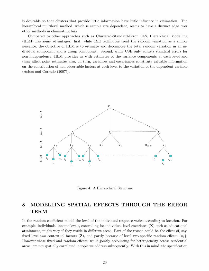
Figure 4 is a diagrammatic representation of a hierarchical structure, with r denoting the top level,g the second level, and I the individual level. There is a varying number of individuals per second levelgroup, and varying numbers of second level groups in each category at the top level of the hierarchy. Inthe context of spatial data we might consider a geographical grouping of individuals with the highestlevel being regions (r) each of which nests smaller geographical sub-regions (g): These sub-regionsmay be either speci�c areas of residence or some other relevant geographical units. Located withineach sub-region there are individuals (I) with a varying number of individuals per sub-region. Weassociate with each individual a response Yi which is dependent upon a set of covariates Xi. However,in assessing whether we might assign any causal relationships between one or more covariates in Xiand the individual response Yi, it is necessary to consider the hierarchical structure of the data, andin particular within- and between-group e¤ects.

There are a number of advantages in taking a multilevel approach. First, in standard unilevelOLS estimation the presence of nested groups of observations may be dealt with by the use of dummyvariables. However, a large number of levels result in a dramatic reduction in degrees of freedom.Second, a multilevel approach helps us to analyze the e¤ect of heterogenous groups in the small samplesituation. In fact with unbalanced data, while OLS estimates of the coe¢ cients give equal weights toeach cluster, the preferred model acknowledges the fact that estimates for the �xed coe¢ cients canchange according to the cluster size. It is therefore possible to adjust both the estimates and theinference according to the precision associated with each group, which is determined by the number ofindividuals in each group (this is technically referred to as shrinkage). In most applications, shrinkage

19

is desirable so that clusters that provide little information have little in�uence in estimation. Thehierarchical multilevel method, which is sample size dependent, seems to have a distinct edge overother methods in eliminating bias.

Compared to other approaches such as Clustered-Standard-Error OLS, Hierarchical Modelling(HLM) has some advantages: �rst, while CSE techniques treat the random variation as a simplenuisance, the objective of HLM is to estimate and decompose the total random variation in an in-dividual component and a group component. Second, while CSE only adjusts standard errors fornon-independence, HLM provides us with estimates of the variance components at each level andthese a¤ect point estimates also. In turn, variances and covariances constitute valuable informationon the contribution of non-observable factors at each level to the variation of the dependent variable(Aslam and Corrado (2007)).

C

r 1 r 2

g 1 g 2 g 3 g 5g 4

I1

I2

I1

I2

g (G ­1 ) g G

Leve

l1Le

ve

l2

I1

I2

r R

2wI1wI3wI

GwII1

I2

Lev

el3

Leve

l4

Figure 4: A Hierarchical Structure

8 MODELLING SPATIAL EFFECTS THROUGH THE ERRORTERM

In the random coe¢ cient model the level of the individual response varies according to location. Forexample, individuals�income levels, controlling for individual level covariates (X) such as educationalattainment, might vary if they reside in di¤erent areas. Part of the reason could be the e¤ect of, say,�xed level two contextual factors (Z), and partly because of level two speci�c random e¤ects fujg.However these �xed and random e¤ects, while jointly accounting for heterogeneity across residentialareas, are not spatially correlated, a topic we address subsequently. With this in mind, the speci�cation

20

of a multilevel model is:Y = �0 +X�1 + Z + " (35)

where Z = fZijg is a set of contextual factors at level-two, Y = fYijg ; X = fXijg and " = feijg+ fujg.The dimension of Y and X and Z are (N � 1), (N � k) and (N � q ) respectively. The vectors �0;�1 and denote the vectors of �xed e¤ect coe¢ cients. The additive error term " is composed ofan idiosyncratic random error term eij for the ith unit belonging to level j and a random e¤ect ujaccounting for some level 2 heterogeneity. We make the following assumptions:

eij jXij � N(0; �e) Cov(eij ; ei0j) = 0; 8i 6= i0uj jXij � N(0; �u) Cov(uj ; eij) = 0

(36)

If we let �2e (�2u) denote the variance of eij (uj) such that for cov(eij ; uj) = 0, then �

2" = �

2e + �

2u

represents the sum, respectively of the within- and between-group variances. Based upon the above,the (equicorrelated) intra-class correlation is:

� =�2u

�2u + �2e

: (37)

This correlation measures the proportion of the variance explained at the group level. In single-levelmodels �2u = 0 and �

2" = �

2e becomes the standard single level residual variance.

In order to accommodate spatial e¤ects operating via the error term we can rewrite the compositeerror term as:

"ij = eij +Xj 6=h

ujWjh; (38)

whereW = fWjhg allows us to specify the way neighboring areas a¤ect uj : The matrix W is a matrixof distances between the G entities as discussed below. The intra-class correlation is now given by:

� =�2uP

j 6=h �2uW

2jh + �

2e

: (39)

Trivially if W = I; where I is the identity matrix, then we have the standard random e¤ects modelignoring any between group e¤ect.

If uj are treated as �xed e¤ects then we need to assume that cov(eij ; uj) = �eu = 0, that istransient individual-level random e¤ects are uncorrelated with, say, a level 2 variable such as the areaof residence. If uj and eij are not independent the Generalized Least Squares (GLS) estimator wouldbe biased and inconsistent. If uj are random e¤ects we also assume independence between these andthe covariates such that cov(Xij ; uj) = �ux = 0 (Blundell and Windmeijer (1997)).

If we �rst rewrite (35) in compact form as:

Y = J�+ �"" (40)

where J is (N � (k + q +1)) and � is ((k + q + 1) � 1) and �" is the design matrix of the randomparameters that is used in the estimation to derive the estimates for b�2e and b�2u: The hierarchicaltwo-stage method for estimating the �xed and random parameters (the variance and covariances ofthe random coe¢ cients) originally proposed by Goldstein (1986),6 is based upon an Iterative LeastSquares (IGLS) method that results in consistent and asymptotically e¢ cient estimates of �:

6The method is currently implemented in the software MLwiN.

21

As Goldstein (1989) has stressed, the IGLS used in the context of random multilevel modellingis equivalent to a maximum likelihood method under multivariate normality which in turn may leadto biased estimates. To produce unbiased estimates a Restricted Iterative Generalized Least Squares(RIGLS) method may be used which, after the convergence is achieved, turns out to be equivalent toa Restricted Maximum Likelihood Estimate (REML). One advantage of the latter method is that, incontrast to IGLS, estimates of the variance components via RIGLS/REML take into account the lossof the degrees of freedom resulting from the estimation of the regression parameters. Hence, whilethe IGLS estimates for the variance components have a downward bias, the RIGLS/REML estimatesdon�t.

9 LINKING SPATIAL MODELS TO HIERARCHICAL MODELSWITH INTERACTION EFFECTS

With the emergence of interaction-based models (Manski (2000), Brock and Durlauf (2001), Akerlof(1997)) research has gradually moved from a pure spatial de�nition of neighborhood towards a multidi-mensional measure based on di¤erent forms of social distance and spillovers (Anselin and Cho (2002),Anselin (1999)). In this setting multilevel models with group e¤ects are generally de�ned as economicenvironments where the payo¤ function of a given agent takes as direct arguments the choice of otheragents (Brock and Durlauf (2001)). A typical example is the emergence of social networks where itis often observed that people belonging to the same group tend to behave similarly (Manski (2000)).The propensity that a person behaves in a certain way varies positively with the dominant behaviorin the group (Bernheim (1994), Kandori (1992)).7

We consider how multilevel models can be linked to spatial models and generalize them to incor-porate more general forms of network dependence involving individuals belonging to the same group.We start by assuming a speci�c form of spatial dependence where the dependent variable, Y, dependson its spatial lag as in traditional spatial autoregressive (SAR) models:

Y = �0 + �WY +X�1+Z + u+ e (41)

whereW is an N�N matrix with G groups/areas each containing wj individuals so thatPGj=1wj = N

and Z is a (N�q )matrix of contextual variables de�ning group characteristics. Let�s start by assumingthatW is a block matrix:

W = Diag(W1; :::;WG) (42)

Wj =1

wj(�wj�

0wj ) j = 1; :::; G

where �wj is the wj-dimensional column vector of ones. Elements in matrixW indicate that individualswithin a group are a¤ected by the (average) behavior of other individuals residing in the same location,in other words by other members of the same group. Figure 5 depicts a situation resembling a completenetwork, as described in Section 3, where each unit Iij i = 1; :::; wj j = 1; :::; G interacts in the sameway with all the other units in the group.

7Other in�uences are the so called peer in�uence e¤ects which have been extensively examined both in education (Bén-abou (1993)), in the psychology literature (Brown (1990) and Brown, Clasen, and Eicher (1986)) and in the occurrenceof social pathologies (Bauman and Fisher (1986); Krosnick and Judd (1982); Jones (1994)).

22

C

r1 r2

g1 g2 g3 g5g4

I1

I2

g(G­1) gG

Leve

l1Le

vel2

rR

1wI

Leve

l3Le

vel4

I3I1

I2

w2II3

I1

I2

GwII3

Figure 5: A Hierarchical Structure: Complete Network within Groups

C

r1 r2

g1 g2 g3 g5g4

I1

I2

g(G­1) gG

Leve

l1Le

vel2

rR

1wI

Leve

l3Le

vel4

I3I1

I2

w2II3

I1

I2

GwII3

Figure 6: A Hierarchical Structure: �Star�within Groups

23

We can envisage many di¤erent form of interactions among members of the same groups. Figure6 illustrates a situation where individuals in the same group are a¤ected by individual I3 withoutin�uencing each other. We can clearly generalize this analysis to other forms of network interactions,such as the nearest neighbor scenario introduced in Section 3 and described by the weight matrixWC ,in which case the block diagonal matrix is:

WC = Diag(WC1 ;W

C1 ; ::;W

CG)

Finally we could also introduce di¤erent type of network structures across groups, further general-izing the structure of the block diagonal matrixWC .

To illustrate the implication of group dependence for spatial models we focus on the hierarchicalcomplete network structure shown in Figure 5. The speci�cation (41) together with the assumptionof group dependence implied by (42) allow us to examine the particular case of a hierarchical modelwhere, for ease of exposition, we assume for the moment that individuals (�rms etc) within the samegroup are a¤ected in the same way by all the other members of the group.

Focussing on within-group e¤ects we therefore assume that �Yj = 1wj

Pwji=1 Yij so that each individual

within group j has the same weight. This means that, somewhat di¤erently from conventional spatialeconometrics, the inter-individual interactions do not spill across group boundaries, and within groupsno account is taken of di¤erential location leading to di¤erent weights according to distance betweenindividuals. We will consider the implication of group spillovers in a hierarchical setting in the followingsection and show how introducing such externalities between groups is crucial for the identi�cation ofnetwork interaction e¤ects.

With this assumption, we can rewrite (41) as:

Yij = �0 + �1 �Yj + �1Xij + Zj + eij + uj (43)

Following Manski (1993), �1 gives the e¤ect of individual level characteristics Xij , �1 captures thestrength of endogenous group e¤ects �Yj , quanti�es the exogenous or contextual e¤ect Zj , uj arerandom group e¤ects and eij is an individual speci�c random component capturing other unmodelledsources of variation in Yij . The problem here is the identi�cation of the parameters in the presenceof what Manski calls re�ection, something which we address below. Of course, identi�cation onlybecomes a problem in linear-in-means models, and any nonlinearity, for instance as in an expandedspatial Durbin model (see Gibbons and Overman (2010)), automatically solves the problem.

As an example, consider workers within companies, with wages Yij dependent on individual workerattributes, Xij ; and on company level contextual e¤ects Zj (such as sector, company wages policy,level of research and development activity, investment etc.). In addition other unmeasured causes ofindividual wage variation are represented by random group (company) e¤ects uj and by individualrandom e¤ects eij ; and with �1 6= 0 wages may also be endogenously determined so that a higher wagelevel achieved by one worker spills over (via �Yj) to other workers in the �rm.

Taking group means of both sides of (43) and solving for �Yj (assuming �1 6= 1) results in thebetween group regression:

�Yj =�0

1� �1+

�11� �1

�Xj +

1� �1Zj + u

0j (44)

where u0j =

�ej+uj1��1

.8 If �Xj = Zj (re�ection), putting together (44) in (43) and centering, we obtain:9

8See Snijders and Bosker (1999, page 53) for the derivation of the between group regression in a multilevel setting.9Technical Appendix A with the proof of equation (45) is available at http://sites.google.com/site/ luisacor-

24

Yij=�0

1� �1+�1 +

1� �1�Xj+�1(Xij � �Xj) + eij+u

00j (45)

with u00j = uj + �1u

0j . This is an example of Manski�s re�ection problem: in situations where group

average characteristics, �Xj , directly a¤ect the individual outcome, Yij ; the parameters in the structuralmodel are not identi�ed. In this case the number of coe¢ cients in the reduced form (45) is notsu¢ cient to identify the coe¢ cients in the structural equation (43). We have four parameters toidentify in the structural equation (43) but only three estimated coe¢ cients in (45). Note that withoutgroup e¤ects (�1 = = 0) the reduced form simpli�es to the basic one-way error component modelYij = �0 + �1Xij + uj + eij . In other words group e¤ects generate excess between group variance byintroducing mean peer characteristics, �Xj ; as an e¤ect on outcomes.10

In the following section we will show how the connection between spatial models and multilevelmodels with group interactions (�1 6= 0; 6= 0), allows parameter identi�cation using simple instru-ments for the endogenous e¤ects, �Yj .

9.1 Spatial E¤ects and Identi�cation

Extending the work by Cohen-Cole (2006) to the area of modelling interaction e¤ects in a multilevelsetting (see Corrado (2009)) we can rewrite (43) in a way that takes into account possible interdepen-dencies not only within groups but also across groups, where a group may be those living in a speci�cdistrict or region. We assume intra-group e¤ects �Yj = 1

wj

Pwji=1 Yij where �Yj is an average of all wj unit

responses within group j and, importantly we now introduce out-group e¤ects �Yl which are equal to anaverage of the responses across all �neighboring�groups, except group j. Typically we might consider�Yl to be based only on those groups that are spatially or socially proximate. Note that thus far theliterature has assumed that all surrounding groups enter with the same weight, but in this paper weintroduce the innovation of di¤erential weighting. Similarly we introduce out-group contextual e¤ects�Zl; thus leading to the model:

Yij = �0 + �1 �Yj + �2( �Yj � �Yl) + �1Xij+ (Zj � �Zl) + eij + uj ; (46)

in which the outcome of individual i in group j, Yij ; depends on the average outcome of group j, wherethe implicit assumption is that unit i is a¤ected equally by all other units in j.

We also assume that the individual outcome depends on the average outcome, �Yl; and averagecontextual e¤ects, �Zl; of other groups �surrounding�group j: We represent the endogenous out-groupsspillover variable in deviation form, as the mean within the group minus the mean in regions �nearby�,hence the variable is �Yj � �Yl. Likewise the contextual spillover variable is speci�ed as Zj � �Zl: In orderto identify all the relevant parameters in the model we consider the average relationship derived from(46):

�Yj =1

1� �1 � �2��0 + �1 �Xj+ (Zj � �Zl)� �2 �Yl

�+ u

0j (47)

rado/publications.10By allowing for the possibility that the conditional mean of group e¤ect and the individual e¤ect vary with group size,

Graham (2008) also allows for the possibility that peer-group e¤ects may di¤er according to class size, being stronger inbigger classes. A way to detect the presence of group e¤ects in this case is to measure the excess between-group variance

de�ned as the ratio of unconditional (scaled) between-group and within group variances EV =E[wj(Y j��y)2]

Eh(wj�1)

�1Pwji=1(Yij�Y j)

2i :

25

where u0j =

�ej+uj1��1��2

.11

Putting together (47) in (46) and assuming re�ection so that Zj = �Xj :

Yij =�0

1� �1 � �2+ �1Xij +

�1(�1 + �2) +

1� �1 � �2�Xj (48)

� �21� �1 � �2

�Yl �

1� �1 � �2�Zl + eij + u

00j

where u00j = uj + (�1 + �2)u

0j . It is clear from (48) that we can identify all the parameters in the

structural equation (46) if the number of level-one units (typically number of individual people) exceedsthe number of groups and @Yij

@ �Yl6= 0;

@Yij@ �Zl

6= 0 i.e. if for some j 6= l agents in one group are a¤ectedby the value of Y or by contextual e¤ects Z in other surrounding groups. Hence one could use outergroups�behaviour as instruments to identify the endogenous e¤ects, �Yj : For example, in the wageequation one could use as instruments wage and company characteristics in neighbouring companies,in other sectors, or at di¤erent geographical/hierarchical levels.

One important issue is collinearity, but the collinearity between Xij and �Xj can be nulli�ed bycentering the variables. Reparameterizing, we obtain an equivalent hierarchical model:12

Yij =�0

1� �1 � �2+ (Xij � �Xj)within-group exogenous

�1 + (49)

� �21� �1 � �2

out-group endogenous

�Yl + + �1

1� �1 � �2between-group exogenous

�Xj �

1� �1 � �2out-group contextual

�Zl + eij + u00j

So we �nd that if we have an HLM model speci�cation that includes out-group e¤ects �Yl and �Zl , thenthis facilitates identi�cation (c.f. Manski, 1993) of the model parameters in equation (46) because wecan use �Yl; �Zl and �Xj as instruments for the endogenous variable �Yj . In doing this we assume thatour instruments are not weak, and are orthogonal to Y.

9.2 Estimating Group Spillovers in Hierarchical Models

The speci�cations developed thus far in fact embody speci�c W matrix assumptions (as describedbelow). Given these, we could envisage a generalization of (49) in order to incorporate more generalforms of group interaction e¤ects:

Y = (I� (�1 + �2)W)�1 (�0��2WlY +WX(�1 + )�WlZ ) + (X�WX)�1 + u00+e (50)

which resembles the spatial Durbin speci�cation (30) in Section 4 whereW is the matrix which de�nesthe within-group e¤ects andWl the out-group e¤ects. Hence, when estimating the simpler speci�cationwhereWlZ =WlY = 0 not only we are unable to identify both endogenous and exogenous interactione¤ects, we also face an omitted variable problem. In this case unobserved (omitted) covariates wouldbe correlated with the observed (included) covariates. Since the observed covariates also include theendogenous spatial lag parameter �2, its signi�cance would be misleading, since it would pick up thee¤ects of the omitted variables WlZ and WlY. This occurrence is particularly problematic when

11Spatial autocorrelation in the error term exists because Yij depends on uj which also a¤ects �Yj and ( �Yj� �Yl) throughthe coe¢ cients �1 and �2.12Technical Appendix B with the proof of equation (49) is available at http://sites.google.com/site/ luisacor-

rado/publications.

26

estimating models with random e¤ects since the maintained assumptions are that both the individualand the group error components should be uncorrelated with the regressors Cov (u;X) = 0 andCov (e;X) = 0: This assumption is of course the same as for random e¤ects panel models, as wouldtypically be tested by means of a Hausman test of parameter consistency. This involves comparison of�xed and random e¤ects estimates, assuming the �xed e¤ects are consistent by being independent ofthe idiosyncratic disturbances. In the hierarchical case omitting spatial e¤ects forX and Z will likewisecreate inconsistent estimators since the error components will be correlated with the regressors.

While we do not have a test that is equivalent to the Hausman test, we do have a way of avoidinginconsistency resulting from omitted variables. This is by means of the inclusion of spatial e¤ectsWlZ and WlY: In fact these play a dual role: (i) of avoiding the omitted variable problem that maya­ ict models with endogenous spatial lags and (ii) of introducing a source of exogenous variation thathelps to identify both endogenous and exogenous group e¤ects, which seems to be vital to most of theempirical work on network interactions. In the context of model (50) estimation of both the observedand unobserved components is achieved via RIGLS/REML, as mentioned in Section 9, given WlY;

WlZ andWX.We now consider a simulation exercise. The basis of this is the group set-up. Groups can be

unequal in size, and the weights do not have to be equal as in equation (42), so that group memberscan carry di¤erential weights, for example, for a 4 member group:

W1 =

264 a b c d

a b c d

a b c d

375 (51)

in which a + b + c + d = 1. Thus W1 can have a di¤erent number of members and di¤erent weights(also summing to 1 across rows), compared withW2,...,WG where G is the number of groups.

This leads to our square diagonalW matrix, which is

W =

266666664

W1 0 0 0 0 0

0 W2 0 0 0 0

0 0 : 0 0 0

0 0 0 : 0 0

0 0 0 0 : 0

0 0 0 0 0 WG

377777775in which 0 stands for a sub-matrix of 0s of appropriate dimension.

The spatial lagging matrix Wl identi�es the location and strength of spillovers between groups,such as for example:

Wl =

266666664

0 W2 0 0 : 0 0

W1 0 0 0 : 0 0

0 0 0 W4 : 0 0

0 0 W3 0 : 0 0

0 0 0 0 : 0 WG

0 0 0 0 : WG�1 0

377777775Given this, we start by considering a generalization of the structural equation (46):

Y = �0�+�1WY+�2(WY �WlY) +X�1 + (Z�WlZ) + u+ e (52)

27

We can therefore simulate our data from the following process for Y:13

Y = (I� (�1 + �2)W+�2Wl)�1 (�0�+X�1 + (Z�WlZ) + u+ e) (54)

We assume that we have 8 groups composed of six members each so that G = 8, N = 6 and thematrices of interactions within each group are assumed to take the form of (51) with values for rowtotals summing to one. Given the matrices W1;W2;...,W8 we therefore de�ne the block matricesof within and between group interactions W and Wl. The value of Y is assumed to depend on anexogenous variableX, on the contextual variable Z; and on the random disturbances e � N(0;2e); andu � N(0;2u) while I is an identity matrix of dimension N . The values of the N by one vectors Z andX are set exogenously; e and u are N by 1 vectors of normally distributed pseudorandom numbers forthe individual and the group random e¤ects which are independent of the exogenous regressors. Given�0 = 0:5; �1 = 0:6; = 0:5; �1 = 0:5 and �2 = 0:9 we generate Y via (54). We ensure throughout that(I� (�1 + �2)W+�2Wl) is non-singular.14

Table 5. Hierarchical Model Estimates for Simulated Data(RIGLS/REML)

Model A Model BCoe¢ cient s:e: Coe¢ cient s:e:

�0 = 0:5 -0.045 0.275 -6.028 0.146�1 = 0:6 0.589 0.007 0.589 0.000 = 0:5 0.479 0.011 -0.114 0.065�1 = 0:5 0.507 0.010 0.761 0.000�2 = 0:9 0.873 0.021 - -

�2u 0.129 0.092 41.11 26.02�2e 0.008 0.001 0.008 0.001N 48 48ll 13.05 1.388

Having generated Y using (54), we estimate two models. One is the correctly speci�ed model (52),denoted model A in Table 5, and the second, model B, is the misspeci�ed model which omits thespatially dependent variableWlY; since �2 = 0; and the out group e¤ect,WlZ. Thus:

Y = �0�+�1WY+�1X+ Z+ u+ e (55)

The estimation via REML reported in Table 5 shows that when we incorrectly �t a DGP omittingthe out-group e¤ectsWlY andWlZ, this causes us to overstate the e¤ect of the endogenous lagWY

as is apparent in the upwardly biased estimate of �1. In addition the in�ated value of the estimatedrandom e¤ects parameter �2u might also be because it is also capturing an omitted variable, so that

13Note that the same result can also be obtained by simulating Y from the reduced from (50):

Y = (I� (�1 + �2)W+�2Wl)�1 ��0�+WX(�1 + )�WlZ

�+ (X�WX)�1 + u

00+e (53)

where u00= u+ ((�1 + �2)W��2Wl)u

0and u

0= (I� (�1 + �2)W+�2Wl)

�1 (We+ u) :14The code to generate the data for the estimations in Table 5 is available at http://personal.strath.ac.uk/

bernard.�ngleton/.

28

it is not a truly (unobserved) group e¤ect. Therefore care must be taken in HLM estimation whenassuming group independence.

10 CONCLUSIONS

We ask the question, �Where is the economics in spatial econometrics?�. Our answer is that economictheory is to be found underpinning many spatial econometric models, but it is evident that when itcomes to the so-calledW matrix, the economic foundation of many models is at its weakest. Modelingspatial interaction in the economic context means in many cases modelling externalities and spillovers.These are elusive and di¢ cult to pin down, which is probably why we have considerable di¢ culties inde�ning the structure ofW unambiguously. The di¢ culty of detecting and measuring spatial spilloverphenomena was recognized by Krugman (1991), who famously remarked that knowledge �ows �leave nopaper trail by which they can be measured or tracked, and there is nothing to prevent the theorist fromassuming anything about them that she likes�. We have called for a stronger more theoretical basisforW to supplement the very signi�cant atheoretical empirical foundations that dominate, somethingthat might emerge from current work on games, network formation, dynamics and equilibria that isoccurring within the social science, notably within the economics of networks. We have attempted toshow that the concept of theW matrix is however undeniably necessary in one form or another andis in any case almost inescapable. It �rst comes to our attention as a convenient, useful and succinctrepresentation of spatial interaction, either in the form of endogenous or exogenous lagged variables,and/or as part of an explicit error process.

However we also �nd that the W matrix has a pervasive presence extending far beyond cross-sectional models to multi-equation models and panel data models. The denial ofW does not completelyeliminate it, merely suppresses it only to reappear as assumptions about distance and interaction incompeting or complementary approaches, with a few exceptions, such as seemingly unrelated regres-sion, vector autoregressions and vector error correction models applied to multivariate time series.Moreover, we have shown that it exists not only trivially in implied form in autoregressive time seriesprocesses, but is, we now discover, a cognate part of hierarchical models. We have considered in somedetail the connection between hierarchical models and the standard spatial econometric speci�cations,because hierarchical models are almost completely absent from the spatial econometrics literature, andrepresent one major alternative way of capturing spatial e¤ects, focussing on the multilevel aspectsof causation that are a reality of many spatial processes. Our contribution in this regard is to showthatW appears also in a speci�c form as part of the structure of hierarchical models. This highlightsthe limitations of much of current hierarchical modelling, which should bene�t from cross-fertilizationfrom the spatial econometrics literature, with the prospect of a whole new research agenda embodyingdi¤erential spatial dependence within and between groups in the multilevel context.

References

[1] Akerlof, George A. (1997). �Social Distance and Social Decisions,�Econometrica, 65, pp. 1005�1028.

[2] Andrews, Donald (1991). �Heteroskedasticity and Autocorrelation Consistent Covariance Matrix Estimation,�

Econometrica, 59, pp. 817�858.

[3] Anselin, Luc (1986). �Non-nested Tests on the Weight Structure in Spatial Autoregressive Models,� Journal ofRegional Science, 26, pp. 267�284.

29

[4] � � (1988). Spatial Econometrics: Methods and Models. The Netherlands: Kluwer Academic Publishers.

[5] � � (1999). �The Future of Spatial Analysis in the Social Sciences,�Geographic Information Sciences, 5, pp. 67�76.

[6] � � (2003). �Spatial Externalities,�International Regional Science Review, 26, pp. 147�152.

[7] � � (2010). �Thirty Years of Spatial Econometrics,�Papers in Regional Science, 89, pp. 3�25.

[8] Anselin, Luc, and Wendy K. T. Cho (2002). �Spatial E¤ects and Ecological Inference,�Political Analysis, 10, pp.276�303.

[9] Anselin, Luc, Julie Le Gallo and Hubert Jayet (2007). �Spatial Panel Econometrics,�in L. Matyas and P. Sevestre(eds.), The Econometrics of Panel Data, Fundamentals and Recent Developments in Theory and Practice. Dordrecht:

Kluwer, 3rd Edition, pp. 625-660.

[10] Anselin, Luc and Rosina Moreno (2003). �Properties of Tests for Spatial Error Components,�Regional Science andUrban Economics, 33, pp. 595�618.

[11] Aslam, Aqib and Luisa Corrado (2007). �No Man is An Island: The Inter-personal Determinants of Regional Well-Being in Europe,�Cambridge Working Papers in Economics 0717, Faculty of Economics, University of Cambridge.

[12] Baltagi, Badi H. and Dong Li (2006). �Prediction in the Panel Data Model with Spatial Correlation: The Case ofLiquor,�Spatial Economic Analysis, 1, pp. 75�185.

[13] Barde, Sylvain (2010). �Increasing Returns and the Spatial Structure of French Wages,�Spatial Economic Analysis,5, pp. 73�79.

[14] Bauman, Karl, and Lynn Fisher (1986). �On the Measurement of Friend Behavior in Research on Friend In�uenceand Selection: Findings from Longitudinal Studies of Adolescent Smoking and Drinking,� Journal of Youth and

Adolescence, 15, pp. 345�353.

[15] Bénabou, Roland (1993). �Workings of a City: Location, Education, and Production,�Quarterly Journal of Eco-nomics, CVIII, pp. 619�652.

[16] Bernheim, Douglas (1994). �A Theory of Conformity,�Journal of Political Economy, 102, pp. 841�877.

[17] Bhattacharjee, Arnab and Sean Holly (2006). �Taking Personalities out of Monetary Policy Decision Making? Inter-actions, Heterogeneity and Committee Decisions in the Bank of England MPC,�Centre for Dynamic Macroeconomic

Analysis Working Paper Series 0612, School of Economics and Finance, University of St. Andrews.

[18] Blundell, Richard and Frank Windmeijer (1997). �Correlated Cluster E¤ects and Simultaneity in Multilevel Models,�Health Economics, 1, pp. 6�13.

[19] Bodson, Paul and Dominique Peters (1975). �Estimation of the Coe¢ cients of a Linear Regression in the Presenceof Spatial Autocorrelation: An Application to a Belgium Labor Demand Function,�Environment and Planning, 7,

pp. 455�472.

[20] Brock, William A. and Stephen N. Durlauf (2001). �Interactions-Based Models,�in J. J. Heckman, and E. Leamer

(eds), Handbook of Econometrics, Vol. 5. Amsterdam: Elsevier Science, pp. 3297�3380.

[21] Brown, Bradford (1990). �Peer Groups and Peer Cultures,�in S. Feldman, and G. Elliott (eds.), At the Threshold:the Developing Adolescent, Cambridge MA: Harvard University Press, pp. 171-196.

30

[22] Brown, Bradford, Donna Clasen and Sue Eicher (1986). �Perceptions of Peer Pressure, Peer Conformity Dispositionsand Self-Reported Behavior Among Adolescents,�Developmental Psychology, 22, pp. 521�530.

[23] Bryk, Anthony S. and Stephen W. Raudenbush (1992). Hierarchical Linear Models for Social and Behavioral Re-search: Applications and Data Analysis Methods. Newbury Park CA: Sage Publications.

[24] Burridge, Peter and Bernard Fingleton (2010). �Bootstrap Inference in Spatial Econometrics : the J Test,�SpatialEconomic Analysis, 5, pp. 93�119.

[25] Chang, Sheng-Wen and Edward Coulson (2001). �Sources of Sectoral Employment Fluctuations in Central Citiesand Suburbs: Evidence from Four Eastern U.S. Cities,�Journal of Urban Economics, 49, pp. 199-218.

[26] Cli¤, Andrew D. and John K. Ord (1973). Spatial Autocorrelation. London: Pion.

[27] � � (1981). Spatial Processes: Models and Applications. London: Pion.

[28] Cohen-Cole, Ethan (2006). �Multiple Groups Identi�cation in the Linear-in-Means Model,�Economics Letters, 92,pp. 157�162.

[29] Conley, Timothy G. (1999). �GMM Estimation with Cross-Sectional Dependence,�Journal of Econometrics, 92, pp.

1�45.

[30] Conley, Timothy G. and Ethan Ligon (2002). �Economic Distance, Spillovers and Cross Country Comparisons,�Journal of Economic Growth, 7, pp. 157�187.

[31] Conley, Timothy G. and Giorgio Topa (2002). �Socio-economic Distance and Spatial Patterns in Unemployment,�Journal of Applied Econometrics, 17, pp. 303�327.

[32] Corrado, Luisa (2009). �A Uni�ed Solution to the Identi�cation and Estimation of Social Interaction E¤ects,�mimeo.

[33] Corrado, Luisa and Bernard Fingleton (2010). �Multilevel Modelling with Spatial E¤ects,�mimeo.

[34] Cressie, Noel (2003). Statistics for Spatial Data. New York: Wiley.

[35] Ertur, Cem and Wilfried Koch (2007). �Growth, Technological Interdependence and Spatial Externalities: Theory

and Evidence,�Journal of Applied Econometrics, 22, pp. 1033�1062.

[36] Fingleton, Bernard (2001). �Equilibrium and Economic Growth: Spatial Econometric Models and Simulations,�

Journal of Regional Science, 41, pp. 117�147.

[37] � � (2003). �Increasing Returns: Evidence from Local Wage Rates in Great Britain,�Oxford Economic Papers, 55,

pp. 716�739.

[38] � � (2006). �The New Economic Geography versus Urban Economics: an Evaluation using Local Wage Rates in

Great Britain,�Oxford Economic Papers, 58, pp. 501�530.

[39] � � (2008). �A Generalized Method of Moments Estimator for a Spatial Model with Moving Average Errors, with

Application to Real Estate Prices,�Empirical Economics, 34, pp. 35�57.

[40] � � (2009). �Spatial Autoregression,�Geographical Analysis, 41, pp. 385�391.

[41] Fingleton, Bernard and Julie Le Gallo (2008). �Estimating Spatial Models with Endogenous Variables, a SpatialLag and Spatially Dependent Disturbances: Finite Sample Properties,�Papers in Regional Science, 87, pp. 319�339.

31

[42] � � (2009). �Endogeneity in a Spatial Context : Properties of Estimators,�in A. Páez, J. Le Gallo, R. Buliung, and

S. Dall�Erba. (eds.), Progress in Spatial Analysis: Theory and Computation, and Thematic Applications, Advances

in Spatial Sciences. Berlin: Springer-Verlag, pp. 59�73.

[43] Fingleton, Bernard and Enrique Lopez-Bazo (2006). �Empirical Growth Models with Spatial E¤ects,�Papers inRegional Science, 85, pp. 177�198.

[44] Folmer, Henk and Johan Oud (2008). �How to Get Rid of W: a Latent Variables Approach to Modelling SpatiallyLagged Variables,�Environment and Planning A, 40, pp. 2526�2538.

[45] Gibbons, Stephen, and Henry Overman (2010). �Mostly Pointless Spatial Econometrics?,� Journal of RegionalScience, forthcoming.

[46] Goldstein, Harvey (1986). �Multilevel Mixed Linear Model Analysis Using Iterative Generalised Least Squares,�Biometrika, 73, pp. 46�56.

[47] � � (1989). �Restricted Unbiased Iterative Generalized Least-Squares Estimation,�Biometrika, 76, pp. 622�623.

[48] � � (1998). �Multilevel Models for Analysing Social Data,�in Encyclopaedia of Social Research Methods. Newbury

Park CA: Sage Publications.

[49] Goyal, Sanjeev (2009). Connections: an Introduction to the Economics of Networks. Princeton: Princeton UniversityPress.

[50] Graham, Bryan S. (2008). �Identifying Social Interactions through Conditional Variance Restrictions,�Econometrica,76, pp. 643�660.

[51] Greenhut, Melvyn, Goerge Norman and Chao-Shun Hung (1987). The Economics of Imperfect Competition: ASpatial Approach. Cambridge: Cambridge University Press.

[52] Harris, Richard, John Mo¤at and Victoria Kravtsova (2010). �In Search of W,�mimeo.

[53] Holly, Sean, M. Hashem Pesaran and Takashi Yamagata (2010). �Spatial and Temporal Di¤usion of House Prices

in the UK,�Journal of Urban Economics, forthcoming.

[54] Hsiao, Cheng and M. Hashem Pesaran (2008). �Random Coe¢ cient Panel Data Models,� in L. Matyas and P.

Sevestre (eds.), The Econometrics of Panel Data: Fundamentals and Recent Developments in Theory and Practice.

Third Edition. Berlin: Springer Publishers, pp. 185-213.

[55] Jones, Andrew (1994). �Health, Addiction, Social Interaction, and the Decision to Quit Smoking,�Journal of HealthEconomics, 13, pp. 93�110.

[56] Kandori, Michihiro (1992). �Social Norms and Community Enforcement,� Review of Economic Studies, 59, pp.

63�80.

[57] Kapetanios, George and M. Hashem Pesaran (2005). �Alternative Approaches to Estimation and Inference in Large

Multifactor Panels: Small Sample Results with an Application to Modelling of Asset Results,�in G.D.A. Phillips, and

E. Tzavalis (eds.), The Re�nement of Econometric Estimation and Test Procedures: Finite Sample and Asymptotic

Analysis. Cambridge: Cambridge University Press, pp. 239-281.

[58] Kapoor, Mudit, Harry H. Kelejian, and Ingmar R. Prucha (2007). �Panel Data Models with Spatially CorrelatedError Components,�Journal of Econometrics, 140, pp. 97�130.

32

[59] Kelejian, Harry H. (2008). �A Spatial J-test for Model Speci�cation against a Single or a Set of Non-Nested Alter-natives,�Letters in Spatial and Resource Sciences, 1, pp. 3�11.

[60] Kelejian, Harry H. and Ingmar R. Prucha (1998). �A Generalized Spatial Two-Stage Least Squares Procedure for

Estimating a Spatial Autoregressive Model with Autoregressive Disturbances,�Journal of Real Estate Finance and

Economics, 17, pp. 99�121.

[61] � � (2007). �HAC estimation in a Spatial Framework,�Journal of Econometrics, 140, pp. 131�154.

[62] Kelejian, Harry H. and Dennis P. Robinson (1995). �Spatial Correlation: A Suggested Alternative to the Autoregres-sive Model,�in L. Anselin, and R. Florax (eds.), New Directions in Spatial Econometrics. Berlin: Springer-Verlag,

pp. 75-95.

[63] Krosnick, Jon A., and Charles M. Judd (1982). �Transitions in Social In�uence in Adolescence: Who InducesCigarette Smoking,�Developmental Psychology, 81, pp. 359�368.

[64] Krugman, Paul (1991). Geography and Trade. Cambridge, MA: MIT Press.

[65] Leenders, Roger T. A. J. (2002). �Modeling Social Infuence through Network Autocorrelation: Constructing theWeight Matrix,�Social Networks, 24, pp. 21�47.

[66] LeSage, James and Manfred Fischer (2008). �Spatial Growth Regressions: Model Speci�cation, Estimation andInterpretation,�Spatial Economic Analysis, 3, pp. 275�304.

[67] LeSage, James and Kelley R. Pace (2008). �Spatial Econometric Modeling of Origin-Destination Flows,�Journal ofRegional Science, 48, pp. 941�967.

[68] � � (2009). Introduction to Spatial Econometrics. Boca Raton, FL: CRC Press.

[69] LeSage, James and Olivier Parent (2007). �Bayesian Model Averaging for Spatial Econometric Models,�GeographicalAnalysis, 39, pp. 241�267.

[70] LeSage, James and Anna Krivelyova (1999). �A Spatial Prior for Bayesian Autoregressive Models,� Journal of

Regional Science, 39, pp. 297�317.

[71] Longford, Nicholas T. (1993). Random Coe¢ cient Models. London: Claredon Press.

[72] Manski, Charles F. (1993). �Identi�cation of Endogenous Social E¤ects: The Re�ection Problem,�Review of Eco-nomic Studies, 60, pp. 531�542.

[73] � � (2000). �Economic Analysis of Social Interactions,�Journal of Economic Perspectives, 3, pp. 115-136.

[74] McFadden, Daniel (1974). �Conditional Logit Analysis of Qualitative Choice Behavior,� in P. Zarembka (eds.),Frontiers in Econometrics. New York: Academic, pp. 105�142.

[75] � � (1979). �Qualitative Methods for Analysing Travel Behaviour of Individuals: some Recent Developments,�in

S. Hensher (eds.), Behaviour Travel Modelling. London: Croom Helm, pp. 279�318.

[76] McMillen, Daniel P. (2010a). �Issues in Spatial Data Analysis,�Journal of Regional Science, 50, pp. 119�141.

[77] � � (2010b). �Perspectives on Spatial Econometrics: Linear Smoothing with Structural Models,�Journal of Regional

Science, forthcoming.

33

[78] Moulton, Brent R. (1986). �Random Group E¤ects and the Precision of Regression Estimates,�Journal of Econo-

metrics, 32, pp. 385�397.

[79] � � (1990). �An Illustration of a Pitfall in Estimating the E¤ects of Aggregate Variables on Micro Unit,�The

Review of Economics and Statistics, 72, pp. 334�338.

[80] Ord, John K. (1975). �Estimation Methods for Models of Spatial Interaction,�Journal of the American StatisticalAssociation, 70, pp. 120�126.

[81] Pace, Kelley R. and James LeSage (2008). �Omitted Variable Bias of OLS and Spatial Lag Models,�in A. Páez, J.Le Gallo, R. Buliung, and S. Dall�Erba. (eds.), Progress in Spatial Analysis: Theory and Methods and Thematic

Applications. Berlin: Springer, pp. 17-28.

[82] Paci, Ra¤aele and Stefano Usai (2009). �Knowledge Flows across European Regions,�Annals of Regional Science,43, pp. 669�690.

[83] Parent, Olivier and James LeSage (2008). �Using the Variance Structure of the Conditional Autoregressive Speci�-cation to Model Knowledge Spillovers,�Journal of Applied Econometrics, 23, pp. 235�256.

[84] Patuelli, Roberto, Aura Reggiani, Sean P. Gorman, Peter Nijkamp, and Franz-Josef Bade (2007). �Network Analysisof Commuting Flows: A Comparative Static Approach to German Data,�Networks and Spatial Economics, 7, pp.

315�331.

[85] Pesaran, M. Hashem (2007). �A Simple Panel Unit Root Test in the Presence of Cross-Sectional Dependence,�

Journal of Applied Econometrics, 138, pp. 2265�2312.

[86] Pinkse, Joris and Margaret E. Slade (2010). �The Future of Spatial Econometrics,�Journal of Regional Science, 50,pp. 103�1117.

[87] Pinkse, Joris, Margaret E. Slade, and Craig Brett (2002). �Spatial Price Competition: a Semiparametric Approach,�Econometrica, 70, pp. 1111�1153.

[88] Slade, Margaret E. (2005). �The Role of Economic Space in Decision Making,�ADRES Lecture, Annales D�Èconomieet De Statistique, 77, pp. 1-20.

[89] Snijders, Tom and Roel Bosker (1999), Multilevel Analysis: an Introduction to Basic and Advanced Multilevel

Modeling, London: Sage Publications.

[90] Smith, Tony E. and James LeSage (2004). �A Bayesian Probit Model with Spatial Dependencies,�in J. LeSage andR. Pace (eds.), Advances in Econometrics, Volume 18: Spatial and Spatiotemporal Econometrics. Oxford: Emerald

Group Publishing, pp. 127�160.

[91] Wilson, Alan G. (1967). �A Statistical Theory of Spatial Distribution Models,� Transportation Research, 1, pp.

253�269.

[92] � � (1970). Entropy in Urban and Regional Modelling. London: Pion.

34

Spatial Economics Research Centre (SERC)London School of EconomicsHoughton StreetLondon WC2A 2AE

Tel: 020 7852 3565Fax: 020 7955 6848Web: www.spatialeconomics.ac.uk

SERC is an independent research centre funded by theEconomic and Social Research Council (ESRC), Departmentfor Business Innovation and Skills (BIS), the Department forCommunities and Local Government (CLG) and the WelshAssembly Government.