Munich Personal RePEc Archive

Where is an oil shock?

Engemann, Kristie and Owyang, Michael T. and Wall,

Howard J.

1 June 2011

Online at https://mpra.ub.uni-muenchen.de/31383/

MPRA Paper No. 31383, posted 09 Jun 2011 20:49 UTC

0

Where is an Oil Shock?*

Kristie M. Engemann

Federal Reserve Bank of St. Louis

Michael T. Owyang

Federal Reserve Bank of St. Louis

Howard J. Wall†

ISEE, Lindenwood University

June 1, 2011

Abstract

Much of the literature examining the effects of oil shocks asks the question ―What is an

oil shock?‖ and has concluded that oil-price increases are asymmetric in their effects on

the US economy. That is, sharp increases in oil prices affect economic activity adversely,

but sharp decreases in oil prices have no effect. We reconsider the directional symmetry

of oil-price shocks by addressing the question ―Where is an oil shock?‖, the answer to

which reveals a great deal of spatial/directional asymmetry across states. Although most

states have typical responses to oil-price shocks—they are affected by positive shocks

only—the rest experience either negative shocks only (5 states), both positive and

negative shocks (5 states), or neither shock (5 states).

Keywords: State-Level Oil Shocks

JEL codes: C31, E37, R12

* The views expressed are those of the authors and do not necessarily represent official positions of the

Federal Reserve Bank of St. Louis or the Federal Reserve System. We would like to thank Lutz Kilian and

John Elder for their comments and suggestions. † Corresponding Author: Howard Wall; ISEE, School of Business and Entrepreneurship; Lindenwood

University; 209 S. Kingshighway; St. Charles, MO 63301. E-Mail: hwall@lindenwood.edu.

1

1. Introduction

Oil-price shocks are often viewed as one of the primary exogenous causes of

national macroeconomic fluctuations. Hamilton (2005), for example, suggests that nine

of the ten recessions in the United States between 1945 to 2005 were preceded by large

positive increases in oil prices.1 Despite the preeminence of sharply increasing oil prices

in advance of recessions, however, large decreases in oil prices have not tended to be

followed by abnormally high national growth. This fact has led to a general acceptance

that oil-price shocks are directionally asymmetric: Large positive oil-price shocks matter,

but negative ones do not. Given the consensus view, studies have, for the most part,

simply imposed directional asymmetry while focusing on the best ways to implement oil-

price shocks into empirical models.2 Hamilton (2003), titled ―What is an Oil Shock?‖, is

a prominent representative of these efforts.

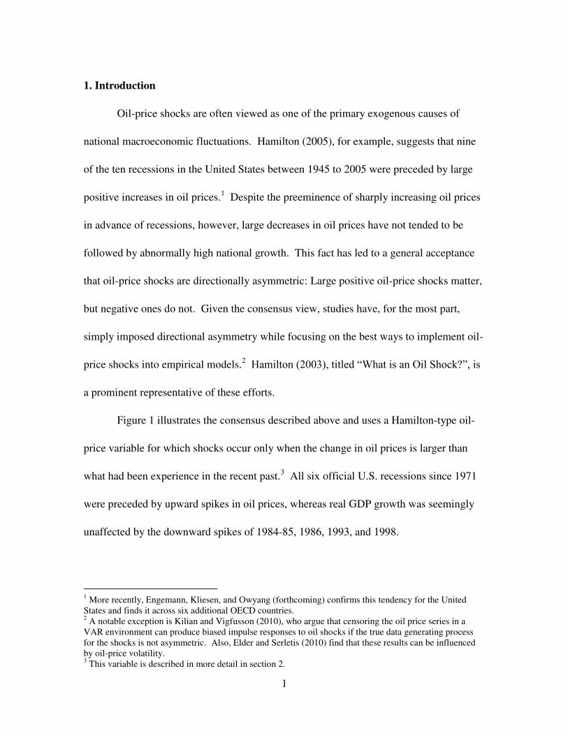
Figure 1 illustrates the consensus described above and uses a Hamilton-type oil-

price variable for which shocks occur only when the change in oil prices is larger than

what had been experience in the recent past.3 All six official U.S. recessions since 1971

were preceded by upward spikes in oil prices, whereas real GDP growth was seemingly

unaffected by the downward spikes of 1984-85, 1986, 1993, and 1998.

1 More recently, Engemann, Kliesen, and Owyang (forthcoming) confirms this tendency for the United

States and finds it across six additional OECD countries. 2 A notable exception is Kilian and Vigfusson (2010), who argue that censoring the oil price series in a

VAR environment can produce biased impulse responses to oil shocks if the true data generating process

for the shocks is not asymmetric. Also, Elder and Serletis (2010) find that these results can be influenced

by oil-price volatility. 3 This variable is described in more detail in section 2.

2

As our title suggests, our interest is in the locations of the effects of oil-price

shocks. Specifically, we reexamine the consensus on oil-price shocks in the context of

state-level business cycles. Our focus on the ―where‖ of oil-price shocks is motivated by

recent studies finding that state-level business cycles can differ a great deal from each

other and from that of the country as a whole. In particular, energy-producing states and

their neighbors have tended to experience idiosyncratic recessions following negative oil-

price shocks, while often not experiencing the recessions seen at the national level

(Owyang, Piger, and Wall, 2005; Crone, 2005; and Hamilton and Owyang, forthcoming).

Figure 2, which compares oil-price shocks to the state recessions determined by

Owyang, Piger, and Wall (2005) for 1979-2002, illustrates the potential variety across

states in the relationship between oil prices and the business cycle. The top panel shows

Figure 1. National Recessions and Oil-Price Shocks

NBER recessions are shaded gray; Dark gray columns are real GDP

growth; Black line is a Hamilton-type oil-price shock variable.

-15

-10

-5

0

5

10

15

-60

-40

-20

0

20

40

60

19

71

19

72

19

73

19

74

19

75

19

76

19

77

19

78

19

79

19

80

19

81

19

82

19

83

19

84

19

85

19

86

19

87

19

88

19

89

19

90

19

91

19

92

19

93

19

94

19

95

19

96

19

97

19

98

19

99

20

00

20

01

20

02

20

03

20

04

20

05

20

06

20

07

20

08

Ha

mil

ton

Oil

-Pric

eS

ho

ck

, P

ercen

t C

ha

ng

e

Rea

l G

DP

Gro

wth

, P

ercen

t

3

Figure 2. State Recessions and Oil-Price Shocks

OPW (2005) state-level recessions are shaded gray. Black

line is a Hamilton-type oil-price shock variable.

0

0.1

0.2

0.3

0.4

0.5

0.6

0.7

0.8

0.9

1

-60

-40

-20

0

20

40

60

19

79

19

80

19

81

19

82

19

83

19

84

19

85

19

86

19

87

19

88

19

89

19

90

19

91

19

92

19

93

19

94

19

95

19

96

19

97

19

98

19

99

20

00

20

01

20

02

North Carolina

0

0.1

0.2

0.3

0.4

0.5

0.6

0.7

0.8

0.9

1

-60

-40

-20

0

20

40

60

19

79

19

80

19

81

19

82

19

83

19

84

19

85

19

86

19

87

19

88

19

89

19

90

19

91

19

92

19

93

19

94

19

95

19

96

19

97

19

98

19

99

20

00

20

01

20

02

Texas

0

0.1

0.2

0.3

0.4

0.5

0.6

0.7

0.8

0.9

1

-60

-40

-20

0

20

40

60

19

79

19

80

19

81

19

82

19

83

19

84

19

85

19

86

19

87

19

88

19

89

19

90

19

91

19

92

19

93

19

94

19

95

19

96

19

97

19

98

19

99

20

00

20

01

20

02

New Mexico

4

that North Carolina‘s experience was largely in line with that of the U.S., although North

Carolina‘s 1990-92 recession began just prior to the sharp rise in oil prices that preceded

the national recession. The middle panel of Figure 2 shows that Texas, a prominent

energy-producing state, had a distinctly idiosyncratic business cycle, especially with

regard to the role of oil prices. Specifically, Texas was in recession in 1979, but did not

go into recession in 1980 or the early 1990s. It did, however, go into recession following

the negative price shock of 1986. Finally, although Texas did experience a recession

following the positive price shocks of 1980-81, it did not do so until nearly a full year

after the start of the national recession. Of the three states illustrated in Figure 2, New

Mexico was the most unfortunate in that it tended to experience recessions following

both positive and negative oil-price shocks. Further, its recovery from recession in 1996

coincided with a sharp increase in oil prices. As with Texas, the role of oil in New

Mexico‘s business cycle does not fit very well with the consensus view.

Our statistical approach follows Hamilton (2003), although we allow for positive

and negative oil-price shocks. After applying the model to each state individually, we

consider several variations on the notion of directional symmetry, all of which indicate

that the usual result is far from the rule across states. For example, only 21 states pass a

standard test for directional asymmetry, which is that the sums of the coefficients on

positive and negative shocks are not statistically the same. After these test for the

existence of positive and negative shocks, we look at the relative magnitudes of their

effects across states and find similarly diverse results. For example, when we look at

5

whether or not there is any significant response for at least one quarter following a shock,

the states fall into four categories: Although 35 states experience only positive shocks,

five see only negative shocks, another five see both positive and negative shocks, and the

remaining five see neither shock.

In addition to estimating the state-by-state effects of oil-price shocks, our analysis

provides general insights into the effects of oil prices by considering 51 macroeconomic

responses rather than one. Further, our use of state-level data has at least one technical

advantage over the use of national-level data alone. Specifically, with national data there

is a potentially serious endogeneity problem because the typical assumption is that oil-

price shocks are exogenous and caused by events external to the U.S. economy (Barsky

and Kilian, 2004; Killian 2008a, 2008b, and 2009). Given the size and importance of the

U.S. economy, this assumption is obviously problematic. In contrast, our assumption that

the world oil price is exogenous at the state level requires significantly less credulity.

We should note several papers that have investigated state or regional

heterogeneity in the responses to oil-price shocks, although none is adequate for

addressing the questions we address. Three have applied VARs to a handful of states and

allowed for positive oil-price shocks only (Penn, 2006; Iledare and Olatubi, 2004; and

Bhattacharya, 2003). Others merely imputed state effects from industry-level results

rather than looking at actual states (Davis, Loungani, and Mahidhara, 1997; Brown and

Yücel, 1995), while still others have derived regional effects from measures of resource

dependence (Brown and Hill, 1988).

6

The balance of the paper is structured as follows: Section 2 describes the model

and presents national-level empirical results that serve as a benchmark. Section 3 uses

state-level data and considers spatial asymmetries in the responses to oil. Section 4

summarizes and concludes.

2. Empirical Implementation

A common approach to modeling the effect of oil-price shocks is to use a

bivariate, single-equation model of GDP, where GDP growth is determined by lags of

itself and past innovations to oil prices. Because output data are not available at a

suitable frequency for states, we use payroll employment. Specifically, we model the

growth rate in state i’s employment, Δyit, as an AR(4):

4

1

4

1

4

1

4

1

4

1

,, )1(,,j

itjtij

j

jtij

j j j

jtijjtiijjtiijiit DixxYyy

where it ~ ),0( 2

iN , and jtx and

jtx are oil-price shocks whose directions are

denoted by their superscripts. The preceding formulation allows us to measure potential

asymmetric responses of state-level economic variables to oil shocks through the

coefficients γij and κij. In (1), jtiY , is the weighted growth rate of employment for all

states excluding state i, and Dt-j is an indicator variable that takes on a value of 1 for the

post-Hurricane-Katrina period. Obviously, (1) represents some restrictions on the cross-

state relationships. Specifically, as in Carlino and DeFina (1998 and 1999), the model

7

does not allow a complete set of cross-state correlations, except through the jtiY , , so

we estimate a separate specification for each state.

In Hamilton's (1983) original paper, oil shocks are defined as the log change in oil

prices under the implicit assumption that the effect of oil shocks on economic activity

was symmetric—i.e., jj . This condition was relaxed in Mork (1989), who

modeled potential asymmetries but utilized the same log change in oil prices as the

baseline shock. These approaches assume that small innovations in oil prices affect

economic activity proportionately to large changes. On the other hand, one might believe

that economic agents do no change their behavior in the presence of small fluctuations in

oil prices, so Hamilton (1996; 2003) and others assume that the effects of oil price shocks

are not only asymmetric but nonlinear. Hamilton (2003) shows that the best-fit model is

one in which oil price shocks only have effects if the rise in prices is substantial—i.e., if

the current (quarterly) price of oil rises above the maximum over the last year.4 Thus, we

define an oil-price shock as

)2(,},,max{

ln100,0max41

xx

x x

tt

tt

which assumes that only increases in oil prices affect economic activity. Similarly, a

negative oil-price shock is defined as

)3(.},,min{

ln100,0min41

xx

x x

tt

tt

4 Hamilton uses the last month of the quarter as the quarterly oil price and Hamilton (2008) uses a three-

year window and argues that the fit is better.

8

We estimate equation (1) first for the United States and then for each of the 50

states plus the District of Columbia. Our measure of oil prices is the producer's price

index for oil, although WTI yields similar results. Our benchmark estimate of (1) uses

the log change of seasonally-adjusted quarterly non-farm payroll employment for the

United States for 1961.1 to 2008:4. Note that several studies have documented a change

over time in the relationship between oil and the macroeconomy (Blanchard and Galí,

2010; Blanchard and Riggi, 2009). To allow for this, we estimate a one-time structural

break in the relationship between oil and national employment growth using a relatively

standard sup-Wald test (Andrews 1993) and find a structural break at 1973:4. This break

coincides with the Arab oil embargo and the emergence of a OPEC as an active cartel.

Our regression results are provided in Table 1. Note that because there were no

negative price shocks during the pre-break period it is not possible to estimate their effect

for that sub-sample. For the full sample and the post-break sample, it is clear that the

relationship between employment growth and oil prices is distinctly different depending

on the direction of the oil-price shock. For both samples, employment growth has a

statistically significant negative response two, three, and four quarters after a positive oil-

price shock, but no such response occurs following negative oil-price shocks. More

formally, the usual directional asymmetry, whereby only positive price shocks matter, is

indicated for a state if 0j but 0j . A higher statistical hurdle for

asymmetry is a failure to reject that jj . As Table 2 shows, directional

symmetry is rejected by both criteria for the full sample and the post-break sample.

9

Table 1. Regression Results, Dependent Variable = Quarterly U.S. Employment Growth Variable jty

jtx

jtx

Lag j = 1 j = 2 j = 3 j = 4 j = 1 j = 2 j = 3 j = 4 j = 1 j = 2 j = 3 j = 4

Coefficient β1

β2

β3

β4

γ1 γ2

γ3 γ4

κ1 κ2

κ3 κ4

α

Full Sample,

1961:2-2008:4

0.879 * -0.189 † 0.089 -0.092 0.001 -0.008 * -0.010 * -0.010 * 0.001 -0.001 -0.001 0.000 0.210 *

(0.076)

(0.103)

(0.102)

(0.072)

(0.004)

(0.004)

(0.004)

(0.004)

(0.004)

(0.004)

(0.004)

(0.004)

(0.038)

Pre-Break,

1961:2-1973:3

0.856 * -0.170 -0.001 -0.116 0.017 -0.061 -0.044 -0.009

0.337 *

(0.165)

(0.220)

(0.216)

(0.150)

(0.028)

(0.045)

(0.046)

(0.046)

(0.092)

Post-Break,

1973:4-2008:4

0.892 * -0.206 † 0.112 -0.094 0.001 -0.007 † -0.009 * -0.009 * 0.000 -0.001 -0.001 0.000 0.180 *

(0.090)

(0.123)

(0.124)

(0.088)

(0.004)

(0.004)

(0.004)

(0.004)

(0.004)

(0.004)

(0.004)

(0.004)

(0.044)

Numbers in parentheses are standard errors. Statistical significance at the 5 percent and 10 percent levels are indicated by ‗*‘ and ‗†‘.

Table 2. Tests of Aggregate Directional Symmetry

H0:

0 i

0 i ii

i

F(.) i F(.)

F(.)

Full Sample -0.028 20.05 * 0.000 0.00

7.61 *

Pre-Break -0.097 1.83

Post-Break -0.025 13.77 * -0.002 0.09

4.41 *

Statistical significance at the 5 percent level is indicated by ‗*‘.

10

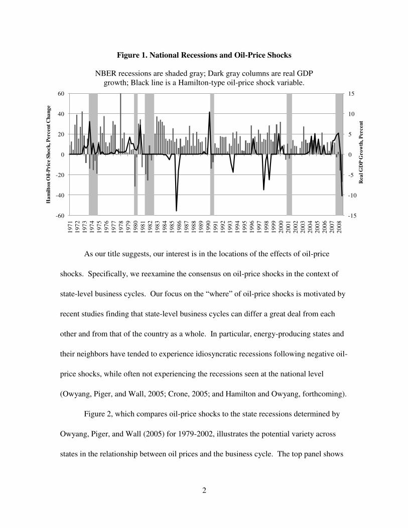
Using the estimated coefficients reported in Table 1, we generate impulse

responses and evaluate positive and negative price shocks in terms of the depth and

frequency of their effects. Figure 3 displays the impulse responses for the post-break

period and yield the typical results: Employment growth is reduced by a positive oil-

price shock for several quarters before returning to normal, but a negative shock has no

statistically significant effect on employment growth. Although we used U.S.

employment rather than GDP as our measure of economic activity, our results are

generally consistent with the existing literature on the effects of oil-price shocks.

Figure 3. U.S. Employment Growth Response to Oil-Price Shocks, Post-Break

3. The Spatial/Directional Asymmetry of Oil-Price Shocks

In this section, we demonstrate that the state-level analogue of the analysis

performed above yields a great deal of heterogeneity in the effects of oil-price shocks.

We explore this spatial/directional asymmetry from two complementary perspectives: the

-0.4

-0.3

-0.2

-0.1

0.0

0.1

0 4 8 12 16 20

Positive Shock Negative Shock

-0.4

-0.3

-0.2

-0.1

0.0

0.1

0 4 8 12 16 20

11

estimated coefficients on the oil-price shock variables and the impulse responses to oil-

price shocks.

3.1. Spatial/Directional Asymmetry I: Oil-Price Shock Coefficients

We performed 51 independent estimations of equation (1) for the post-break

period, the results of which are are analogous to those in Table 1 for the U.S. and are

provided in an appendix. As in the previous section for U.S. data, these estimates are

summarized in Table 3 with the same tests for directional asymmetry that were

performed using national data (Table 2). We find 37 states for which the sum of the

coefficients on a positive price shock ( j ) is negative and statistically significant. Not

only are there 12 states for which j is statistically no different from zero, but for two

states—North Dakota and Wyoming—it is positive and statistically significant. On the

other hand, there is near unanimity in the lack of statistical significance for j . The

exceptions are Delaware and Wyoming, which have opposite signs on j . Finally, as

shown in the final column of Table 3, directional symmetry cannot be rejected for 30

states. Thus, the blanket observation that oil-price shocks have asymmetric effects on

economic activity appears to be false at this level of disaggregation.

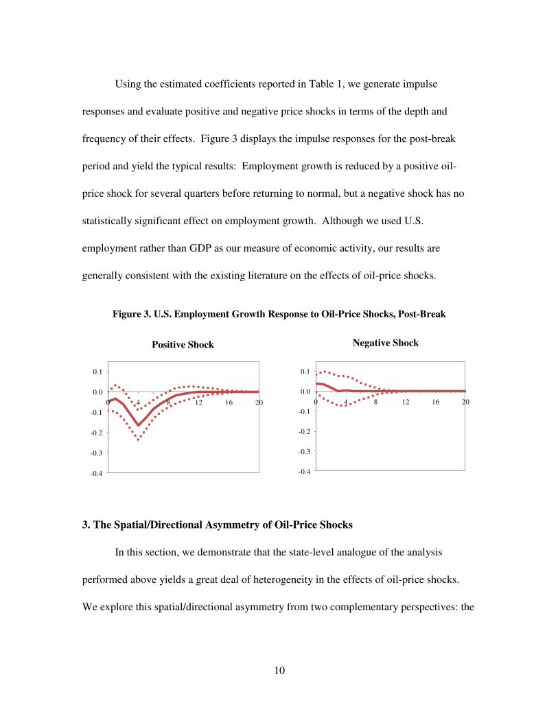
To get an idea of the geographic distribution of the magnitudes of the effects of

oil-price shocks, we map the estimates for the positive-shock coefficients (Figure 4). For

the most part, the nonconforming states—for which the sums of these coefficients are

positive or not statistically significant—are energy states as determined by the relative

12

Table 3. The Spatial/Directional Asymmetry

of Oil-Price Shocks, 1973:4-2008:4

H0:

0 i

0 i ii

i

F(.) i F(.)

F(.)

AK 0.038 1.58

0.039 1.53

0.00 AL -0.030 7.52 * 0.010 0.74

5.10 *

AR -0.046 13.98 * 0.008 0.34

7.22 * AZ -0.053 15.45 * 0.013 0.84

9.10 *

CA -0.030 11.12 * 0.002 0.04

4.92 * CO -0.010 0.89

0.003 0.05

0.57

CT -0.028 8.24 * 0.002 0.03

3.44 † DC -0.017 1.44

-0.006 0.15

0.24

DE -0.051 10.60 * -0.037 5.68 * 0.34 FL -0.026 7.65 * -0.003 0.09

2.35

GA -0.053 18.77 * 0.003 0.07

8.46 * HI -0.013 1.15

-0.014 1.10

0.00

IA -0.018 3.09 † -0.014 1.69

0.05 ID -0.045 8.61 * -0.004 0.06

2.53

IL -0.022 6.23 * -0.006 0.40

1.25 IN -0.058 17.67 * -0.001 0.01

7.22 *

KS -0.005 0.16

0.012 0.96

0.80 KY -0.034 6.14 * -0.010 0.49

1.24

LA 0.006 0.16

0.025 2.14

0.69 MA -0.022 5.24 * 0.000 0.00

1.97

MD -0.039 12.70 * -0.006 0.28

3.48 † ME -0.029 5.36 * -0.020 2.11

0.22

MI -0.072 19.90 * 0.003 0.04

9.49 * MN -0.021 5.07 * -0.010 0.93

0.54

MO -0.042 13.43 * -0.003 0.08

5.12 * MS -0.047 14.81 * 0.012 0.90

9.02 *

MT -0.013 0.84

0.010 0.41

0.97 NC -0.048 16.66 * -0.010 0.64

4.19 *

ND 0.023 3.81 † 0.004 0.11

1.05 NE -0.025 5.07 * 0.016 1.84

5.21 *

NH -0.023 2.76 † -0.001 0.01

0.96 NJ -0.024 5.76 * -0.012 1.18

0.59

NM -0.013 1.71

0.018 2.57

3.51 † NV -0.043 8.09 * -0.010 0.40

1.83

NY -0.020 6.93 * -0.007 0.67

1.09 OH -0.042 14.67 * -0.008 0.54

3.87 †

OK 0.018 1.48

0.022 2.27

0.05 OR -0.061 24.35 * 0.006 0.22

11.28 *

PA -0.020 6.30 * -0.013 2.25

0.32 RI -0.051 10.41 * -0.001 0.00

4.06 *

SC -0.057 16.63 * -0.007 0.20

4.77 * SD -0.010 0.78

-0.004 0.08

0.13

TN -0.054 21.12 * -0.005 0.19

7.04 * TX 0.004 0.16

0.014 1.95

0.60

UT -0.009 0.93

0.015 2.17

2.46 VA -0.038 15.99 * -0.008 0.66

3.72 †

VT -0.016 1.97

-0.011 0.86

0.08 WA -0.034 8.06 * 0.006 0.26

4.50 *

WI -0.031 10.97 * -0.008 0.69

2.29 WV -0.006 0.03

0.018 0.26

0.20

WY 0.037 3.26 † 0.056 5.54 * 0.33 Statistical significance at the 5 percent and 10 percent

levels are indicated by ‗*‘ and ‗†‘, respectively.

13

importance of energy production in their economies (Snead, 2009).5 Most of these states

lie in the vast swath running from the western Gulf coast through Montana. The

exceptions are the non-energy states of Hawaii and Vermont.

3.2. Spatial/Directional Asymmetry II: Impulse Responses

The preceding subsection looked at spatial asymmetries in oil-price shocks from

the perspective of the shocks‘ estimated coefficients. A different perspective can be

gained from the state-level impulse responses to the shocks, which are generated via the

estimated coefficients. Figure 5 provides the post-break responses to positive and

negative oil-price shocks for five representative states: three with variants of the typical

directional asymmetry—California, Kansas, and Michigan—and two with atypical

responses—New Mexico and Wyoming.

5 As determined by Snead (2009), the 13 energy producing states are Alaska, Colorado, Kansas, Louisiana,

Mississippi, Montana, New Mexico, North Dakota, Oklahoma, Texas, Utah, West Virginia, and Wyoming.

Figure 4. Positive Oil-Price Shock

Sum of State γijs

Post-Break, 1973:4 - 2008:4

US = -0.025

-0.072 to -0.032-0.032 to -0.018Not Significant0.023 to 0.037

14

-0.40

-0.20

0.00

0.20

0 4 8 12 16 20

California

-0.40

-0.20

0.00

0.20

0 4 8 12 16 20

Kansas

-0.40

-0.20

0.00

0.20

0 4 8 12 16 20

California

-0.40

-0.20

0.00

0.20

0 4 8 12 16 20

Kansas

-0.40

-0.20

0.00

0.20

0 4 8 12 16 20

Michigan

-0.40

-0.20

0.00

0.20

0 4 8 12 16 20

Michigan

-0.40

-0.20

0.00

0.20

0 4 8 12 16 20

N.Mexico

-0.40

-0.20

0.00

0.20

0 4 8 12 16 20

N.Mexico

-0.40

-0.20

0.00

0.20

0 4 8 12 16 20

Wyoming

-0.40

-0.20

0.00

0.20

0 4 8 12 16 20

Wyoming

Figure 5. Responses to Oil-Price Shocks, Post-Break, Selected States

Positive Price Shock Negative Price Shock

15

Unsurprisingly, given its size and diversity, the response for California is

asymmetric and looks much like that for the United States as a whole (recall Figure 3): A

positive oil-price shock leads to reduced employment growth for several quarters before

returning to normal, but a negative oil-price shock has no effect on employment growth.

Kansas has a negative but bouncy response to a positive oil-price shock, and its response

to a negative oil-price shock is statistically insignificant. Manufacturing-heavy states,

such as Michigan, see a much deeper response to a positive oil-price shocks than does the

country as a whole. On the other hand, because Michigan‘s auto sector likely benefits

from negative oil-price shocks, it has quarters for which the point estimates of its

responses are positive, although not significantly so.

New Mexico is an example of a state with symmetric oil-price responses. As an

energy state, its response to a positive oil-price shock is much like that of Kansas:

negative but bouncy. But, because it is more energy intensive than Kansas, it experiences

a positive and statistically significant response to negative oil-price shocks. This result is

consistent with Figure 2, which showed how New Mexico entered recessions after both

types of oil-price shocks. Our final example is Wyoming, the most energy-intensive state

in the country, which experiences asymmetric responses to oil-price shocks, but not the

typical kind. It sees a statistically significant and huge positive response to negative oil-

price shocks only, but no statistically significant response to a positive oil-price shock.

The states are categorized in Table 4 according to their combination of responses

to oil-price shocks. A state is said to be responsive to a shock if it sees at least one

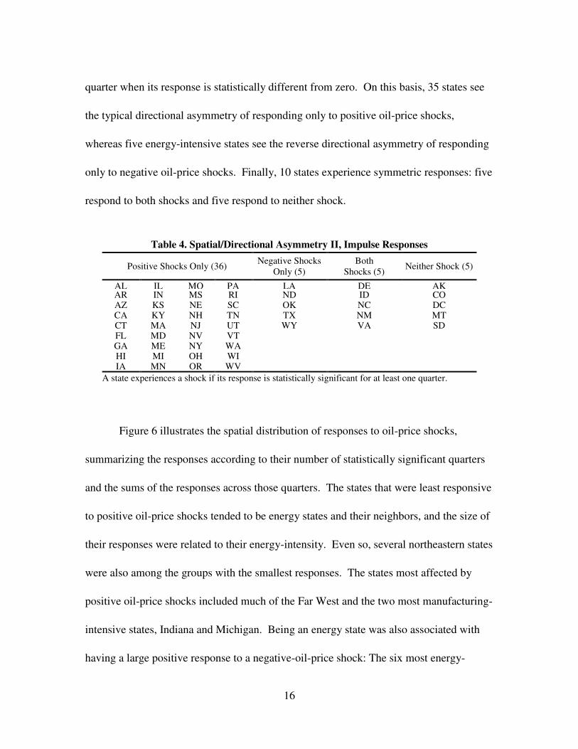
16

quarter when its response is statistically different from zero. On this basis, 35 states see

the typical directional asymmetry of responding only to positive oil-price shocks,

whereas five energy-intensive states see the reverse directional asymmetry of responding

only to negative oil-price shocks. Finally, 10 states experience symmetric responses: five

respond to both shocks and five respond to neither shock.

Table 4. Spatial/Directional Asymmetry II, Impulse Responses

Positive Shocks Only (36) Negative Shocks

Only (5)

Both

Shocks (5) Neither Shock (5)

AL IL MO PA LA DE AK AR IN MS RI ND ID CO AZ KS NE SC OK NC DC CA KY NH TN TX NM MT CT MA NJ UT WY VA SD FL MD NV VT

GA ME NY WA

HI MI OH WI

IA MN OR WV

A state experiences a shock if its response is statistically significant for at least one quarter.

Figure 6 illustrates the spatial distribution of responses to oil-price shocks,

summarizing the responses according to their number of statistically significant quarters

and the sums of the responses across those quarters. The states that were least responsive

to positive oil-price shocks tended to be energy states and their neighbors, and the size of

their responses were related to their energy-intensity. Even so, several northeastern states

were also among the groups with the smallest responses. The states most affected by

positive oil-price shocks included much of the Far West and the two most manufacturing-

intensive states, Indiana and Michigan. Being an energy state was also associated with

having a large positive response to a negative-oil-price shock: The six most energy-

17

intensive states were so affected. On the other hand, there are five non-energy states with

positive responses to negative oil-price shocks, although it was for one quarter only in

each case.

Figure 6. Summary of State Responses to Oil-Price Shocks, Post-Break

4. Conclusions

Nearly all of the literature examining the effects of oil shocks has concluded that

oil-price increases are directionally asymmetric in their effects on the U.S. economy.

Positive Price Shock Negative Price Shock

Number of Significant Quarters

U.S. = 6

0 1 or 23 or 45 or 6

7

Number of Significant Quarters

U.S. = 0

0123

Sum of Significant Quarters

U.S. = -0.56

-1.20 to -0.90-0.90 to -0.70-0.70 to -0.42-0.42 to -0.05

0

Sum of Significant Quarters

U.S. = 0

00.07 to 0.170.19 to 0.39

0.90

18

That is, sharp increases in oil prices affect economic activity adversely, but sharp

decreases in oil prices have no effect. We consider several variations on the notion of

price-shock symmetry, all of which indicate that the usual asymmetry assumption is far

from the rule across states. For example, only 21 states pass a standard test for

directional asymmetry, which is that the sums of the coefficients on positive and negative

shocks are not statistically the same. A similar picture emerges from an analysis of state-

level impulse responses to oil-price shocks. Although most states have typical responses

to oil-price shocks—they experience positive shocks only—the rest experience either

negative shocks only (5 states), both positive and negative shocks (5 states), or neither

shock (5). The magnitudes of the effects shocks also differ a great deal across states.

The most energy-intensive states respond only to negative oil-price shocks and the states

that respond to both shocks are is a mixed bag, including several non-energy states.

19

Appendix. Regression Results, Dependent Variable = Quarterly State Employment Growth

Variable jtiy , jtiY ,

jtx

jtx αi

Lag j = 1 j = 2 j = 3 j = 4 j = 1 j = 2 j = 3 j = 4 j = 1 j = 2 j = 3 j = 4 j = 1 j = 2 j = 3 j = 4

AK 0.365 * 0.114 0.441 * -0.252 * -0.254 0.528 -0.859 † 0.687 † 0.023 0.003 0.012 0.001 0.036 * 0.001 0.003 -0.002 0.149

(0.087)

(0.083

)

(0.082)

(0.084)

(0.368)

(0.503)

(0.503)

(0.359)

(0.018)

(0.018)

(0.019)

(0.019)

(0.018)

(0.019)

(0.019)

(0.018)

(0.213)

AL 0.045 0.119 0.157 0.198 † 1.270 * -1.112 * 0.126 -0.212 0.004 -0.008 -0.008 -0.018 * 0.004 0.005 0.003 -0.002 0.246 *

(0.127)

(0.122

)

(0.112)

(0.111)

(0.201)

(0.244)

(0.267)

(0.200)

(0.006)

(0.007)

(0.007)

(0.007)

(0.007)

(0.007)

(0.007)

(0.007)

(0.070)

AR 0.557 * -0.106 -0.002 0.069 0.466 † -0.565 † 0.158 -0.065 -0.011 -0.002 -0.007 -0.026 * 0.006 -0.004 0.007 -0.001 0.359 *

(0.138)

(0.152

)

(0.150)

(0.126)

(0.251)

(0.301)

(0.305)

(0.229)

(0.007)

(0.008)

(0.008)

(0.008)

(0.008)

(0.008)

(0.008)

(0.008)

(0.080)

AZ 0.324 * 0.372 * 0.129 0.026 0.891 * -1.348 * 0.463 † -0.222 0.011 -0.018 * -0.033 * -0.014 0.004 -0.001 0.011 -0.001 0.353 *

(0.113)

(0.107

)

(0.106)

(0.109)

(0.219)

(0.250)

(0.274)

(0.212)

(0.008)

(0.008)

(0.008)

(0.009)

(0.008)

(0.008)

(0.008)

(0.008)

(0.094)

CA 0.556 * 0.123 0.049 0.137 0.365 * -0.363 * -0.007 -0.044 0.005 -0.013 * -0.009 -0.012 * 0.004 -0.007 0.002 0.003 0.149 *

(0.109)

(0.123

)

(0.116)

(0.106)

(0.143)

(0.165)

(0.165)

(0.129)

(0.005)

(0.005)

(0.006)

(0.006)

(0.005)

(0.005)

(0.005)

(0.005)

(0.056)

CO 0.517 * 0.163 0.142 -0.062 0.456 * -0.443 * 0.168 -0.190 0.006 -0.007 -0.004 -0.004 0.006 0.005 0.002 -0.009 0.183 *

(0.109)

(0.118

)

(0.117)

(0.111)

(0.164)

(0.194)

(0.193)

(0.153)

(0.006)

(0.006)

(0.007)

(0.007)

(0.006)

(0.006)

(0.007)

(0.007)

(0.072)

CT 0.086 0.413 * 0.212 * 0.040 0.758 * -0.572 * -0.002 -0.154 -0.001 -0.001 -0.004 -0.022 * -0.004 -0.002 0.001 0.007 0.108

(0.105)

(0.105

)

(0.106)

(0.105)

(0.152)

(0.202)

(0.204)

(0.160)

(0.006)

(0.006)

(0.006)

(0.006)

(0.006)

(0.006)

(0.006)

(0.006)

(0.068)

DC 0.072 0.184 * 0.153 0.184 † 0.233 -0.159 -0.029 0.068 0.001 -0.005 -0.003 -0.009 0.010 -0.004 0.001 -0.013 0.053

(0.091)

(0.091

)

(0.093)

(0.098)

(0.186)

(0.246)

(0.240)

(0.172)

(0.008)

(0.008)

(0.009)

(0.009)

(0.009)

(0.009)

(0.009)

(0.009)

(0.089)

DE -0.139 0.280 * 0.122 -0.109 0.786 * -0.579 * 0.320 -0.259 -0.014 0.004 -0.017 † -0.024 * 0.000 -0.014 -0.007 -0.016 * 0.341 *

(0.100)

(0.097

)

(0.094)

(0.095)

(0.207)

(0.279)

(0.277)

(0.199)

(0.009)

(0.009)

(0.010)

(0.010)

(0.009)

(0.009)

(0.009)

(0.009)

(0.098)

FL 0.735 * -0.045 0.443 * -0.282 * 0.233 -0.126 -0.371 * 0.097 0.003 -0.010 † -0.010 -0.009 0.006 -0.009 0.005 -0.005 0.233 *

(0.106)

(0.116

)

(0.122)

(0.103)

(0.155)

(0.188)

(0.174)

(0.145)

(0.006)

(0.006)

(0.006)

(0.006)

(0.006)

(0.006)

(0.006)

(0.006)

(0.064)

GA 0.444 * 0.141 0.068 -0.091 0.476 * -0.533 † 0.019 0.111 -0.008 -0.013 † -0.010 -0.021 * 0.005 -0.005 0.002 0.001 0.367 *

(0.132)

(0.138

)

(0.136)

(0.130)

(0.236)

(0.271)

(0.267)

(0.205)

(0.007)

(0.007)

(0.008)

(0.008)

(0.007)

(0.008)

(0.008)

(0.007)

(0.080)

HI 0.182 † 0.286 * 0.360 * -0.138 0.506 * -0.538 * 0.238 -0.059 0.005 -0.001 -0.014 † -0.003 0.006 -0.018 * 0.002 -0.004 0.082

(0.092)

(0.086

)

(0.086)

(0.091)

(0.158)

(0.222)

(0.221)

(0.157)

(0.007)

(0.007)

(0.008)

(0.008)

(0.008)

(0.008)

(0.008)

(0.008)

(0.083)

IA 0.123 0.169 0.534 * -0.052 0.980 * -0.642 * -0.583 * 0.135 0.005 0.003 -0.011 † -0.014 * 0.002 -0.006 -0.002 -0.009 0.144 *

(0.114)

(0.118

)

(0.115)

(0.119)

(0.168)

(0.225)

(0.223)

(0.187)

(0.006)

(0.006)

(0.006)

(0.006)

(0.006)

(0.006)

(0.006)

(0.006)

(0.063)

ID 0.437 * 0.055 0.436 * -0.168 0.469 † -0.835 * 0.058 0.106 0.009 -0.014 -0.023 * -0.017 † 0.000 -0.002 -0.006 0.004 0.341 *

(0.120)

(0.127

)

(0.134)

(0.123)

(0.265)

(0.346)

(0.336)

(0.241)

(0.009)

(0.009)

(0.010)

(0.010)

(0.010)

(0.010)

(0.010)

(0.010)

(0.106)

IL 0.047 0.167 0.202 * -0.259 * 0.926 * -0.096 -0.426 * 0.217 -0.006 0.001 0.003 -0.020 * 0.001 -0.008 -0.004 0.005 -0.038

(0.099)

(0.101

)

(0.101)

(0.095)

(0.134)

(0.193)

(0.197)

(0.167)

(0.005)

(0.005)

(0.006)

(0.006)

(0.005)

(0.005)

(0.005)

(0.005)

(0.061)

IN 0.055 0.164 0.121 0.002 1.231 * -0.845 * -0.033 -0.178 -0.010 -0.020 * -0.009 -0.019 * 0.004 -0.003 -0.001 -0.002 0.273 *

(0.134)

(0.140

)

(0.136)

(0.126)

(0.253)

(0.320)

(0.325)

(0.259)

(0.008)

(0.008)

(0.008)

(0.009)

(0.008)

(0.008)

(0.008)

(0.008)

(0.084)

KS 0.102 0.209 † 0.204 † -0.073 0.809 * -0.409 † -0.304 0.179 0.008 -0.011 0.002 -0.003 0.002 0.003 0.005 0.002 0.148 †

(0.115)

(0.112

)

(0.111)

(0.113)

(0.183)

(0.229)

(0.230)

(0.182)

(0.007)

(0.007)

(0.008)

(0.008)

(0.007)

(0.007)

(0.007)

(0.007)

(0.075)

20

Appendix (continued). Regression Results, Dependent Variable = Quarterly State Employment Growth

Variable jtiy , jtiY ,

jtx

jtx αi

Lag j = 1 j = 2 j = 3 j = 4 j = 1 j = 2 j = 3 j = 4 j = 1 j = 2 j = 3 j = 4 j = 1 j = 2 j = 3 j = 4

KY -0.136 0.286 * 0.004 0.159 1.394 * -1.002 * 0.259 -0.261 -0.007 -0.018 * 0.007 -0.015 † 0.006 -0.011 0.005 -0.011 0.207 *

(0.113)

(0.114)

(0.115)

(0.112)

(0.221)

(0.297)

(0.305)

(0.228)

(0.008)

(0.008)

(0.009)

(0.009)

(0.008)

(0.008)

(0.008)

(0.008)

(0.086)

LA 0.284 * 0.108 0.247 * -0.018 0.609 * -0.320 -0.126 -0.010 0.007 0.000 0.009 -0.009 0.022 * 0.009 -0.002 -0.004 0.077

(0.104)

(0.106)

(0.103)

(0.064)

(0.207)

(0.257)

(0.249)

(0.180)

(0.008)

(0.009)

(0.009)

(0.009)

(0.009)

(0.009)

(0.009)

(0.009)

(0.093)

MA 0.304 * 0.362 * 0.423 * -0.256 * 0.933 * -1.047 * -0.115 0.093 0.006 -0.010 † -0.005 -0.013 * 0.005 -0.002 0.002 -0.005 0.150 *

(0.108)

(0.110)

(0.111)

(0.111)

(0.156)

(0.198)

(0.192)

(0.165)

(0.006)

(0.006)

(0.006)

(0.006)

(0.006)

(0.006)

(0.006)

(0.006)

(0.065)

MD 0.007 0.259 * 0.197 † 0.083 0.611 * -0.202 -0.392 † 0.163 -0.007 -0.014 * -0.010 -0.007 -0.001 -0.002 -0.002 -0.001 0.204 *

(0.111)

(0.111)

(0.110)

(0.111)

(0.169)

(0.216)

(0.213)

(0.163)

(0.006)

(0.006)

(0.007)

(0.007)

(0.007)

(0.007)

(0.007)

(0.007)

(0.069)

ME 0.264 * 0.065 0.101 0.126 0.914 * -0.964 * 0.306 -0.216 0.000 -0.003 -0.018 * -0.008 -0.007 -0.003 -0.003 -0.006 0.203 *

(0.112)

(0.113)

(0.106)

(0.102)

(0.187)

(0.238)

(0.253)

(0.191)

(0.007)

(0.007)

(0.008)

(0.008)

(0.008)

(0.008)

(0.008)

(0.008)

(0.079)

MI 0.236 † 0.030 0.411 * -0.207 0.939 * -0.818 * -0.309 0.289 -0.008 -0.023 * -0.017 † -0.023 * 0.006 0.001 -0.005 0.002 0.251 *

(0.125)

(0.124)

(0.131)

(0.127)

(0.275)

(0.331)

(0.314)

(0.236)

(0.009)

(0.009)

(0.009)

(0.010)

(0.009)

(0.009)

(0.009)

(0.009)

(0.107)

MN 0.110 0.277 * 0.178 0.038 0.846 * -0.551 * 0.041 -0.162 -0.004 -0.006 -0.006 -0.005 -0.003 -0.004 0.003 -0.006 0.154 *

(0.115)

(0.119)

(0.122)

(0.116)

(0.148)

(0.181)

(0.178)

(0.153)

(0.005)

(0.005)

(0.006)

(0.006)

(0.006)

(0.006)

(0.006)

(0.006)

(0.059)

MO 0.017 0.038 0.074 -0.191 0.969 * -0.411 † -0.065 0.230 -0.007 -0.025 * 0.000 -0.010 0.000 -0.009 0.005 0.000 0.159 *

(0.122)

(0.125)

(0.118)

(0.117)

(0.180)

(0.222)

(0.223)

(0.170)

(0.006)

(0.006)

(0.007)

(0.007)

(0.006)

(0.007)

(0.007)

(0.006)

(0.067)

MS 0.517 * 0.133 0.022 -0.070 0.515 * -0.759 * -0.004 0.255 0.004 -0.012 -0.026 * -0.014 0.013 † -0.008 0.001 0.006 0.265 *

(0.125)

(0.132)

(0.129)

(0.119)

(0.216)

(0.248)

(0.259)

(0.209)

(0.007)

(0.007)

(0.008)

(0.008)

(0.007)

(0.008)

(0.008)

(0.008)

(0.079)

MT 0.155 † 0.097 0.184 † 0.142 0.885 * -0.647 * -0.342 0.101 0.004 -0.009 -0.012 0.004 0.014 -0.008 -0.001 0.006 0.247 *

(0.093)

(0.095)

(0.093)

(0.092)

(0.194)

(0.265)

(0.271)

(0.200)

(0.009)

(0.009)

(0.009)

(0.009)

(0.009)

(0.009)

(0.009)

(0.009)

(0.102)

NC 0.432 * 0.151 -0.328 * -0.054 0.574 * -0.668 * 0.657 * -0.116 -0.002 -0.012 † -0.024 * -0.011 -0.001 -0.004 0.001 -0.006 0.335 *

(0.123)

(0.128)

(0.126)

(0.124)

(0.215)

(0.234)

(0.238)

(0.188)

(0.007)

(0.007)

(0.007)

(0.008)

(0.007)

(0.007)

(0.007)

(0.007)

(0.077)

ND 0.236 * 0.220 * 0.079 0.051 0.946 * -1.007 * 0.268 -0.016 0.011 0.003 0.000 0.009 0.015 * -0.009 -0.001 -0.001 0.070

(0.092)

(0.096)

(0.087)

(0.084)

(0.143)

(0.208)

(0.231)

(0.163)

(0.007)

(0.007)

(0.007)

(0.007)

(0.007)

(0.007)

(0.007)

(0.007)

(0.079)

NE 0.119 -0.055 0.138 -0.259 * 0.595 * -0.271 0.012 0.370 * 0.001 -0.005 -0.017 * -0.004 0.008 0.003 0.000 0.005 0.233 *

(0.097)

(0.095)

(0.096)

(0.096)

(0.158)

(0.211)

(0.207)

(0.158)

(0.007)

(0.007)

(0.007)

(0.007)

(0.007)

(0.007)

(0.007)

(0.007)

(0.075)

NH 0.329 * 0.358 * 0.246 * -0.011 0.571 * -0.844 * -0.039 -0.192 -0.003 -0.008 -0.008 -0.004 0.002 -0.002 0.003 -0.004 0.308 *

(0.116)

(0.117)

(0.118)

(0.118)

(0.229)

(0.283)

(0.286)

(0.225)

(0.008)

(0.008)

(0.009)

(0.009)

(0.009)

(0.009)

(0.009)

(0.009)

(0.090)

NJ 0.163 0.374 * 0.054 0.050 0.612 * -0.548 * -0.021 -0.035 -0.001 -0.005 -0.003 -0.014 * -0.002 -0.006 -0.007 0.004 0.142 *

(0.115)

(0.115)

(0.116)

(0.116)

(0.166)

(0.212)

(0.219)

(0.167)

(0.006)

(0.006)

(0.006)

(0.006)

(0.006)

(0.006)

(0.006)

(0.006)

(0.065)

NM 0.282 * 0.095 0.227 * 0.060 0.611 * -0.596 * 0.011 0.023 0.008 -0.019 * -0.005 0.004 0.009 0.003 0.000 0.006 0.242 *

(0.107)

(0.107)

(0.104)

(0.105)

(0.146)

(0.176)

(0.182)

(0.132)

(0.006)

(0.006)

(0.006)

(0.006)

(0.006)

(0.006)

(0.006)

(0.006)

(0.080)

NV 0.444 * 0.256 * 0.132 -0.074 0.522 * -0.660 * 0.290 -0.100 -0.001 -0.023 * -0.010 -0.009 -0.011 0.000 0.002 -0.002 0.348 *

(0.105)

(0.113)

(0.116)

(0.111)

(0.227)

(0.283)

(0.279)

(0.218)

(0.009)

(0.009)

(0.010)

(0.010)

(0.010)

(0.010)

(0.010)

(0.009)

(0.116)

21

Appendix (continued). Regression Results, Dependent Variable = Quarterly State Employment Growth

Variable jtiy , jtiY ,

jtx

jtx αi

Lag j = 1 j = 2 j = 3 j = 4 j = 1 j = 2 j = 3 j = 4 j = 1 j = 2 j = 3 j = 4 j = 1 j = 2 j = 3 j = 4

NY 0.210 † 0.389 * 0.027 0.089 0.512 * -0.428 * 0.110 -0.176 0.004 -0.013 * -0.003 -0.008 -0.003 -0.003 0.004 -0.005 0.082

(0.116)

(0.120)

(0.121)

(0.111)

(0.124)

(0.165)

(0.163)

(0.122)

(0.004)

(0.004)

(0.005)

(0.005)

(0.005)

(0.005)

(0.005)

(0.005)

(0.051)

OH -0.115 -0.074 0.370 * 0.044 1.243 * -0.207 -0.376 -0.146 -0.004 -0.013 * -0.009 -0.015 * -0.002 -0.003 -0.001 -0.001 0.039

(0.131)

(0.132)

(0.133)

(0.135)

(0.212)

(0.273)

(0.262)

(0.221)

(0.006)

(0.006)

(0.007)

(0.007)

(0.007)

(0.007)

(0.007)

(0.007)

(0.084)

OK 0.258 * 0.307 * 0.024 0.011 0.427 * -0.035 -0.094 0.017 0.002 0.010 0.007 -0.001 0.020 * 0.019 * -0.019 * 0.002 0.020

(0.103)

(0.100)

(0.095)

(0.092)

(0.189)

(0.241)

(0.236)

(0.173)

(0.008)

(0.008)

(0.008)

(0.009)

(0.008)

(0.008)

(0.009)

(0.009)

(0.086)

OR 0.576 * 0.010 0.128 0.075 0.223 -0.393 0.051 -0.041 -0.004 -0.013 † -0.025 * -0.019 * 0.000 0.011 -0.004 0.000 0.337 *

(0.124)

(0.135)

(0.131)

(0.114)

(0.220)

(0.265)

(0.257)

(0.193)

(0.007)

(0.007)

(0.008)

(0.008)

(0.008)

(0.008)

(0.008)

(0.008)

(0.079)

PA -0.167 0.271 * -0.012 0.099 0.975 * -0.546 * 0.128 -0.147 0.000 -0.005 -0.006 -0.010 † 0.002 -0.005 0.000 -0.009 † 0.014

(0.109)

(0.112)

(0.112)

(0.111)

(0.135)

(0.188)

(0.187)

(0.149)

(0.005)

(0.005)

(0.005)

(0.005)

(0.005)

(0.005)

(0.005)

(0.005)

(0.059)

RI 0.140 0.029 0.178 -0.103 1.126 * -0.849 * 0.075 -0.101 0.011 -0.020 * -0.012 -0.030 * 0.002 -0.004 0.003 -0.001 0.190 †

(0.107)

(0.112)

(0.109)

(0.106)

(0.248)

(0.328)

(0.331)

(0.248)

(0.009)

(0.010)

(0.010)

(0.010)

(0.010)

(0.010)

(0.010)

(0.010)

(0.103)

SC -0.025 0.032 -0.079 -0.006 1.354 * -0.735 * 0.151 -0.072 0.005 -0.017 * -0.012 -0.033 * -0.001 -0.007 0.006 -0.005 0.373 *

(0.122)

(0.120)

(0.114)

(0.113)

(0.252)

(0.290)

(0.296)

(0.224)

(0.008)

(0.008)

(0.009)

(0.009)

(0.009)

(0.009)

(0.009)

(0.009)

(0.090)

SD 0.121 0.114 0.213 * 0.146 0.945 * -0.549 * -0.185 -0.211 -0.006 0.000 -0.004 -0.001 -0.001 -0.009 0.003 0.003 0.238 *

(0.098)

(0.100)

(0.099)

(0.097)

(0.163)

(0.223)

(0.225)

(0.176)

(0.007)

(0.007)

(0.008)

(0.008)

(0.008)

(0.008)

(0.008)

(0.007)

(0.084)

TN 0.227 0.247 † -0.105 -0.016 0.923 * -0.845 * 0.108 0.008 -0.009 -0.009 -0.011 -0.024 * 0.003 -0.009 0.000 0.001 0.329 *

(0.149)

(0.147)

(0.143)

(0.136)

(0.248)

(0.277)

(0.281)

(0.236)

(0.007)

(0.007)

(0.007)

(0.007)

(0.007)

(0.007)

(0.007)

(0.007)

(0.072)

TX 0.803 * 0.087 -0.279 * 0.099 0.151 -0.185 0.344 * -0.196 † 0.007 -0.001 -0.006 0.004 0.022 * -0.007 -0.001 0.000 0.150 *

(0.106)

(0.128)

(0.129)

(0.107)

(0.135)

(0.158)

(0.144)

(0.110)

(0.005)

(0.005)

(0.005)

(0.006)

(0.005)

(0.006)

(0.006)

(0.006)

(0.058)

UT 0.252 * 0.429 * 0.057 -0.057 0.849 * -0.817 * 0.337 † -0.232 0.005 -0.003 -0.007 -0.004 0.009 -0.005 0.008 0.004 0.230 *

(0.103)

(0.104)

(0.102)

(0.103)

(0.138)

(0.181)

(0.190)

(0.151)

(0.006)

(0.006)

(0.006)

(0.006)

(0.006)

(0.006)

(0.006)

(0.006)

(0.076)

VA 0.119 0.482 * 0.190 -0.223 † 0.623 * -0.683 * 0.052 0.131 -0.005 -0.013 * -0.006 -0.014 * 0.001 -0.006 -0.006 0.002 0.271 *

(0.121)

(0.125)

(0.126)

(0.122)

(0.162)

(0.200)

(0.204)

(0.158)

(0.005)

(0.006)

(0.006)

(0.006)

(0.006)

(0.006)

(0.006)

(0.006)

(0.063)

VT 0.351 * 0.026 0.273 * 0.129 0.562 * -0.352 † -0.209 -0.071 -0.006 -0.009 -0.003 0.002 -0.002 -0.004 0.004 -0.009 0.149 *

(0.115)

(0.114)

(0.113)

(0.114)

(0.171)

(0.209)

(0.209)

(0.164)

(0.007)

(0.007)

(0.007)

(0.007)

(0.007)

(0.007)

(0.007)

(0.007)

(0.073)

WA 0.333 * 0.235 * 0.219 † -0.052 0.291 -0.060 -0.232 0.083 -0.004 -0.009 -0.013 † -0.008 0.005 0.004 -0.001 -0.002 0.233 *

(0.108)

(0.111)

(0.110)

(0.108)

(0.181)

(0.228)

(0.216)

(0.162)

(0.007)

(0.007)

(0.007)

(0.008)

(0.007)

(0.007)

(0.007)

(0.007)

(0.078)

WI 0.037 0.172 0.287 * -0.027 0.904 * -0.470 * -0.181 -0.017 0.000 -0.014 * -0.009 -0.008 0.001 -0.003 -0.006 -0.001 0.186 *

(0.127)

(0.121)

(0.118)

(0.123)

(0.164)

(0.197)

(0.193)

(0.167)

(0.005)

(0.005)

(0.006)

(0.006)

(0.006)

(0.006)

(0.006)

(0.006)

(0.059)

WV -0.395 * -0.072 -0.180 † -0.060 1.740 * -1.184 † 0.799 0.114 -0.034 † 0.012 0.024 -0.008 0.002 0.002 0.010 0.005 -0.201

(0.093)

(0.101)

(0.100)

(0.094)

(0.466)

(0.678)

(0.672)

(0.470)

(0.020)

(0.020)

(0.022)

(0.022)

(0.021)

(0.021)

(0.021)

(0.021)

(0.218)

WY 0.432 * 0.033 0.275 * -0.123 0.668 * -0.003 -0.227 0.001 0.011 0.000 0.031 * -0.005 0.040 * 0.014 0.015 -0.014 0.015

(0.092)

(0.094)

(0.096)

(0.085)

(0.248)

(0.341)

(0.342)

(0.247)

(0.012)

(0.012)

(0.012)

(0.013)

(0.012)

(0.013)

(0.013)

(0.013)

(0.124)

Numbers in parentheses are standard errors. Statistical significance at the 5 percent and 10 percent levels are indicated by ‗*‘ and ‗†‘, respectively.

22

References

Andrews, Donald W.K. ―Tests for Parameter Instability and Structural Change with

Unknown Change Point.‖ Econometrica, July 1993, 61(4), pp. 821-856.

Barsky, Robert B. and Kilian, Lutz. ―Oil and the Macroeconomy Since the 1970s.‖

Journal of Economic Perspectives, Fall 2004, 18(4), pp. 115-134.

Bhattacharya, Radha. ―Sources of Variation in Regional Economies.‖ Annals of Regional

Science, 2003, 37, pp. 291-302.

Blanchard, Olivier J. and Galí, Jordi. ―The Macroeconomic Effects of Oil Price Shocks:

Why Are the 2000s So Different From the 1970s?‖ in J. Galí and M. Gertler, eds.,

International Dimensions of Monetary Policy, University of Chicago Press: Chicago,

2010.

Blanchard, Olivier J. and Riggi, Marianna. ―Why Are the 2000s So Different from the

1970s? A Structural Interpretation of Changes in the Macroeconomic Effects of Oil

Prices.‖ NBER Working Paper 15467, October 2009.

Brown, Stephen P.S. and Yücel, Mine K. ―Energy Prices and State Economic Performance.‖ Federal Reserve Bank of Dallas Economic Review, Second Quarter

1995, pp. 13-23.

Carlino, Gerald and DeFina, Robert. ―The Differential Regional Effects of Monetary

Policy.‖ Review of Economics and Statistics, 1998, 80, pp. 572-587.

Carlino, Gerald and DeFina, Robert. ―The Differential Regional Effects of Monetary

Policy: Evidence from the U.S. States.‖ Journal of Regional Science, 1999, 39, pp.

339-358.

Crone, Theodore M. ―An Alternative Definition of Economic Regions in the United

States Based on Similarities in State Business Cycles.‖ Review of Economics and

Statistics, November 2005, 87(4), pp. 617-626.

Davis, Steven J. and Haltiwanger, John. ―Sectoral Job Creation and Destruction

Responses to Oil Price Changes.‖ Journal of Monetary Economics, December 2001,

48(3), pp. 465-512.

Davis, Steven J.; Loungani, Prakash; and Mahidhara, Ramamohan. ―Regional Labor

Fluctuations: Oil Shocks, Military Spending, and Other Driving Forces.‖ Board of

Governors of the Federal Reserve System, International Finance Discussion Paper

No. 578, March 1997.

Elder, John and Serletis, Apostolos. ―Oil Price Uncertainty.‖ Journal of Money, Credit

and Banking, September 2010, 42(6), pp. 1137–1159.

Engemann, Kristie M.; Kliesen, Kevin L., and Owyang, Michael T. ―Do Oil Shocks

Drive Business Cycles? Some U.S. and International Evidence.‖ Macroeconomic

Dynamics, forthcoming.

Hamilton, James D. ―Oil and the Macroeconomy Since World War II.‖ Journal of

Political Economy, April 1983, 91(2), pp. 228-248.

23

Hamilton, James D. ―What Is an Oil Shock?‖ Journal of Econometrics, April 2003,

113(2), pp. 363-398.

Hamilton, James D. ―Oil and the Macroeconomy.‖ In Steven Durlauf and Lawrence

Blume, eds., New Palgrave Dictionary of Economics, 2nd edition, Palgrave

McMillan Ltd., 2008.

Hamilton, James D. and Owyang, Michael T. ―The Propagation of Regional Recessions.‖

Review of Economics and Statistics, forthcoming.

Iledare, Omowumi and Olatubi, Williams O. ―The Impact of Changes in Crude Oil Prices and Offshore Oil Production on the Economic Performance of U.S. Coastal Gulf

States.‖ Energy Journal, 2004, 25(2), pp. 97-113.

Kilian, Lutz. ―Exogenous Oil Supply Shocks: How Big Are They and How Much Do

They Matter for the U.S. Economy?‖ Review of Economics and Statistics, May

2008a, 90(2), pp. 216-240.

Kilian, Lutz. ―The Economic Effects of Energy Price Shocks.‖ Journal of Economic

Literature, 2008b, 46(4), pp. 871-909.

Kilian, Lutz. ―Not All Oil Shocks Are Alike: Disentangling Demand and Supply Shocks

in the Crude Oil Market.‖ American Economic Review, June 2009, 99(2), pp. 1053-

1069.

Kilian, Lutz and Vigfusson, Robert J. ―Are the Responses of the U.S. Economy

Asymmetric in Energy Price Increases and Decreases?‖ Working Paper, March

2010.

Mork, Knut Anton. ―Oil and the Macroeconomy When Prices Go Up and Down: An

Extension of Hamilton's Results.‖ Journal of Political Economy, June 1989, 97(3),

pp. 740-744.

Owyang, Michael T.; Piger, Jeremy; and Wall, Howard J. ―Business Cycle Phases in U.S.

States.‖ Review of Economics and Statistics, November 2005, 87(4), pp. 604-616.

Penn, David A. ―What Do We Know About Oil Prices and State Economic Performance?‖ Federal Reserve Bank of St. Louis Regional Economic Development,

2006, 2(2), pp. 131-139.

Snead, Mark C. ―Are the Energy States Still Energy States?‖ Federal Reserve Bank of Kansas City Economic Review, Fourth Quarter 2009, pp. 43-68.