Where Are We Now?

Real-Time Estimates of the Macro Economy

Martin D. D. Evans

Georgetown University

and the NBER

March 2005

Forthcoming in

The International Journal of Central Banking

Abstract

This paper describes a method for calculating daily real-time estimates of the current state of the U.S.

economy. The estimates are computed from data on scheduled U.S. macroeconomic announcements using an

econometric model that allows for variable reporting lags, temporal aggregation, and other complications in

the data. The model can be applied to �nd real-time estimates of GDP, in�ation, unemployment or any other

macroeconomic variable of interest. In this paper I focus on the problem of estimating the current level of and

growth rate in GDP. I construct daily real-time estimates of GDP that incorporate public information known

on the day in question. The real-time estimates produced by the model are uniquely-suited to studying how

perceived developments the macro economy are linked to asset prices over a wide range of frequencies. The

estimates also provide, for the �rst time, daily time series that can be used in practical policy decisions.

Keywords: Real-time data, Kalman Filtering, Forecasting GDP

JEL Codes: E37 C32

IntroductionInformation about the current state of real economic activity is widely dispersed across consumers, �rms

and policymakers. While individual consumers and �rms know the recent history of their own decisions,

they are unaware of the contemporaneous consumption, saving, investment and employment decisions made

by other private sector agents. Similarly, policymakers do not have access to accurate contemporaneous

information concerning private sector activity. Although information on real economic activity is collected

by a number of government agencies, the collection, aggregation and dissemination process takes time. Thus,

while U.S. macroeconomic data are released on an almost daily basis, the data represent o¢ cial aggregations

of past rather than current economic activity.

The lack of timely information concerning the current state of the economy is well-recognized among

policymakers. This is especially true in the case of GDP, the broadest measure of real activity. The

Federal Reserve�s ability to make timely changes in monetary policy is made much more complicated by

the lack of contemporaneous and accurate information on GDP. The lack of timely information concerning

macroeconomic aggregates is also important for understanding private sector behavior, and in particular

the behavior of asset prices. When agents make trading decisions based on their own estimate of current

macroeconomic conditions, they transmit information to their trading partners. This trading activity leads

to the aggregation of dispersed information and in the process a¤ects the behavior of asset prices. Evans

and Lyons (2004a) show that the lack of timely information concerning the state of the macroeconomy can

signi�cantly alter the dynamics of exchange and interest rates by changing the trading-based process of

information aggregation.

This paper describes a method for estimating the current state of the economy on a continual basis using

the �ow of information from a wide range of macroeconomic data releases. These real-time estimates are

computed from an econometric model that allows for variable reporting lags, temporal aggregation, and other

complications that characterize the daily �ow of macroeconomic information. The model can be applied to

�nd real-time estimates of GDP, in�ation, unemployment or any other macroeconomic variable of interest.

In this paper, I focus on the problem of estimating GDP in real time.

The real-time estimates derived here are conceptually distinct from the real-time data series studied by

Croushore and Stark (1999, 2001), Orphanides (2001) and others. A real-time data series comprises a set of

historical values for a variable that are known on a particular date. This date identi�es the vintage of the

real-time data. For example, the March 31st. vintage of real-time GDP data would include data releases

on GDP growth up to the forth quarter of the previous year. This vintage incorporates current revisions to

earlier GDP releases but does not include a contemporaneous estimate of GDP growth in the �rst quarter.

As such, it represents a subset of public information available on March 31st. By contrast, the March

31st. real-time estimate of GDP growth comprises an estimate of GDP growth in the �rst quarter based on

information available on March 31st. The real-time estimates derived in this paper use an information set

that spans the history of data releases on GDP and 18 other macroeconomic variables.

A number of papers have studied the problem of estimating GDP at a monthly frequency. Chow and

Lin (1971) �rst showed how a monthly series could be constructed from regression estimates using monthly

data related to GDP and quarterly GDP data. This technique has been subsequently integrated into VAR

forecasting procedures (see, for example, Robertson and Tallman 1999). More recently, papers by Lui and

Hall (2000) and Mariano and Murasawa (2003) have used state space models to combine quarterly GDP

1

data with other monthly series. The task of calculating real-time estimates of GDP growth has also been

addressed by Clarida, Kitchen and Monaco (2002). They develop a regression-based method that uses a

variety of monthly indicators to forecast GDP growth in the current quarter. The real-time estimates are

calculated by combining the di¤erent forecasts with a weighting scheme based on the relative explanatory

power of each forecasting equation.

I di¤er from this literature by modelling the growth in GDP as the quarterly aggregate of an unobserved

daily process for real economy-wide activity. The model also speci�es the relationship between GDP, data

releases on GDP growth, and data releases on a set of other macroeconomic variables in a manner that

accommodates the complex timing of releases. In particular, I incorporate the variable reporting lags that

exist between the end of each data collection period (i.e., the end of a month or quarter) and the release

day for each variable. This is only possible because the model tracks the evolution of the economy on a

daily basis. An alternative approach of assuming that GDP aggregrates an unobserved monthly process

for economy-wide activity would result in a simpler model structure (see, Lui and Hall 2000 and Mariano

and Murasawa 2003), but it could not accommodate the complex timing of data releases. The structure of

the model also enables me to compute real-time estimates of GDP as the solution to an inference problem.

In practice, I obtain the real-time estimates as a by-product of estimating the model. First, the model

parameters are estimated by (qausi) maximum likelihood using the Kalman Filter algorithm. The real-time

estimates are then obtained by applying the algorithm to the model evaluated at the maximum likelihood

estimates.

My method for computing real-time estimates has several noteworthy features. First, the estimates are

derived from a single fully-speci�ed econometric model. As such, we can judge the reliability of the real-time

estimates by subjecting the model to a variety of diagnostic tests. Second, a wide variety of variables can

be computed from the estimated model. For example, the model can provide real-time forecasts for GDP

growth for any future quarter. It can also be used to compute the precision of the real-time estimates as

measured by the relevant conditional variance. Third, the estimated model can be used to construct high

frequency estimates of real-economic activity. We can construct a daily series of real-time estimates for GDP

growth in the current quarter, or real-time estimates of GDP produced in the current month, week, or even

day. Fourth, the method can incorporate information from a wide range of economic indicators. In this

paper I use the data releases for GDP and 18 other macroeconomic variables, but the set of indicators could

be easily expanded to include many other macroeconomic series and �nancial data. Extending the model in

this direction may be particular useful from a forecasting perspective. Stock and Watson (2002) show that

harnessing the information in a large number indicators can have signi�cant forecasting bene�ts.

The remainder of the paper is organized as follows. Section 1 describes the inference problem that must

be solved in order to compute the real-time estimates. Here I detail the complex timing of data collection and

macroeconomic data releases that needs to be accounted for in the model. The structure of the econometric

model is presented in Section 2. Section 3 covers estimation and the calculation of the real-time estimates.

I �rst show how the model can be written in state space form. Then I describe how the sample likelihood

is constructed with the use of the Kalman Filter. Finally, I describe how various real-time estimates are

calculated from the maximum likelihood estimates of the model. Section 4 presents the model estimates

and speci�cation tests. Here I compare the forecasting performance of the model against a survey of GDP

estimates by professional money managers. These private estimates appear comparable to the model-based

2

estimates even though the managers have access to much more information than the model incorporates.

Section 5 examines the model-based real-time estimates. First, I consider the relation between the real-time

estimates and the �nal GDP releases. Next, I compare alternative real-time estimates for the level of GDP

and examine the forecasting power of the model. Finally, I study how the data releases on other macro

variables are related to changes in GDP at a monthly frequency. Section 6 concludes.

1 Real-Time Inference

My aim is to obtain high frequency real-time estimates on how the macro economy is evolving. For this

purpose, it is important to distinguish between the arrival of information and data collection periods. Infor-

mation about GDP can arrive via data releases on any day t: GDP data is collected on a quarterly basis. I

index quarters by � and denote the last day of quarter � by q(�); with the �rst, second and third months

ending on days m(� ; 1); m(� ; 2) and m(� ; 3) respectively. I identify the days on which data is released in

two ways. The release day for variable { collected over quarter � is r{(�): Thus, {r(�) denotes the valueof variable {; over quarter � ; released on day r{(�): The release day for monthly variables is identi�ed byr{(� ; i) for i = 1; 2; 3: In this case, {r(�;i) is the value of {; for month i in quarter � ; announced on dayr{(� ; i): The relation between data release dates and data collection periods is illustrated in Figure 1:

value of ( ,3)Mz τ value of Q( )y τ

Q( )τ released here released hereM( ,1)τ M( ,2)τ M( ,3)τ | M( 1,1)τ + M( 2,2)τ + |

R ( ,3)z τ R ( )y τ

Month 1 Month 2 Month 3 Month 1 Month 2 Month 3Quarter τ Quarter 1τ +

[ ( ,3)Mz τ collected  ][ Q( )y τ  collected                            ]

Figure 1: Data collection periods and release times for quarterly and monthly variables. Thereporting lag for ��nal�GDP growth in quarter � , yq(�); is ry(�)�q(�). The reporting lag for themonthly series zm(�;j) is rz(� ; j)�m(� ; j). for j = 1; 2; 3:

The Bureau of Economic Analysis (BEA) at the U.S. Commerce Department releases data on GDP

growth in quarter � in a sequence of three announcements: The �advanced�growth data are released during

the �rst month of quarter �+1; the �preliminary�data are released in the second month; and the ��nal�data

are released at the end of quarter � +1. The ��nal�data release does not represent the last o¢ cial word on

GDP growth in the quarter. Each summer, the BEA conducts an �annual�or comprehensive revision that

generally lead to revisions in the ��nal�data values released over the previous three years. These revisions

incorporate more complete and detailed micro data than was available before the ��nal�data release date.1

Let xq(�) denote the log of real GDP for quarter � ending on day q(�); and yr(�) be the ��nal� data

1For a complete description of BEA procedures, see Carson (1987), and Seskin and Parker (1998).

3

released on day ry(�): The relation between the ��nal�data and actual GDP growth is given by

yr(�) = �qxq(�) + �r(�); (1)

where �qxq(�) � xq(�) � xq(��1) and �a(�) represents the e¤ect of the future revisions (i.e., the revisionsto GDP growth made after ry(�)): Notice that equation (1) distinguishes between the end of the reporting

period q(�); and the release date ry(�): I shall refer to the di¤erence ry(�)�q(�) as the reporting lag forquarterly data. (For data series { collected during month i of quarter � ; the reporting lag is r{(� ; i)�m(� ; i):)Reporting lags vary from quarter to quarter because data is collected on a calendar basis but announcements

are not made on holidays and weekends. For example, ��nal�GDP data for the quarter ending in March

has been released between June 27 th. and July 3 rd.

Real-time estimates of GDP growth are constructed using the information in a speci�c information set.

Let t denote an information set that only contains data that is publicly known at the end of day t: The

real-time estimate of GDP growth in quarter � is de�ned as E[�qxq(�)jq(�)]; the expectation of �qxq(�)conditional on public information available at the end of the quarter, q(�): To see how this estimate relates

to the ��nal�data release, y; I combine the de�nition with (1) to obtain

yr(�) = E��qxq(�)jq(�)

�+ E

��r(�)jq(�)

�+�yr(�) � E

�yr(�)jq(�)

��: (2)

The ��nal� data released on day ry(�) comprises three components; the real-time GDP growth estimate,

an estimate of future data revisions, E��r(�)jq(�)

�; and the real-time forecast error for the data release,

yr(�)�E�yr(�)jq(�)

�: Under the reasonable assumption that yr(�) represents the BEA�s unbiased estimate

of GDP growth, and that q(�) represents a subset of the information available to the BEA before the release

day, E��r(�)jq(�)

�should equal zero. In this case, (2) becomes

yr(�) = E��qxq(�)jq(�)

�+�yr(�) � E

�yr(�)jq(�)

��: (3)

Thus, the data release yr(�) can be viewed as a noisy signal of the real-time estimate of GDP growth, where

the noise arises from the error in forecasting yr(�) over the reporting lag. By construction, the noise term

is orthogonal to the real-time estimate because both terms are de�ned relative to the same information set,

q(�): The noise term can be further decomposed as

yr(�) � E�yr(�)jq(�)

�=�Ehyr(�)jbeaq(�)

i� E

�yr(�)jq(�)

��+�yr(�) � E

hyr(�)jbeaq(�)

i�; (4)

where beat denotes the BEA�s information set. Since the BEA has access to both private and public

information sources, the �rst term on the right identi�es the informational advantage conferred on the BEA

at the end of the quarter q(�). The second term identi�es the impact of new information the BEA collects

about xq(�) during the reporting lag. Since both of these terms could be sizable, there is no a priori reason

to believe that real-time forecast error is always small.

To compute real-time estimates of GDP, we need to characterize the evolution of t and describe how

inferences about �qxq(�) can be calculated from q(�): For this purpose, I incorporate the information

contained in the �advanced�and �preliminary�GDP data releases. Let yr(�) and ~yr(�) respectively denote

4

the values for the �advanced� and �preliminary� data released on days ry(�) and r~y(�) where q(�) <

ry(�) < r~y(�): I assume that yr(�) and ~yr(�) represent noisy signals of the ��nal�data, yr(�) :

yr(�) = yr(�) + ~er(�) + er(�); (5)

~yr(�) = yr(�) + ~er(�); (6)

where ~er(�) and er(�) are independent mean zero revision shocks. ~er(�) represents the revision between

days ry(�) and ry(�) and er(�) represents the revision between days ry(�) and r~y(�):The idea that the

provisional data releases represent noisy signals of the ��nal�data is originally due to Mankiw and Shapiro

(1986). It implies that the revisions ~er(�) and ~er(�)+ er(�) are orthogonal to yr(�): I impose this orthogonality

condition when estimating the model. The speci�cation of (5) and (6) also implies that the �advanced�

and �preliminary� data releases represent unbiased estimates of actual GDP growth. This assumption is

consistent with the evidence reported in Faust et. al (2000) for US data releases between 1988 and 1997.

(Adding non-zero means for ~er(�) and er(�) is a straightforward extension to accommodate bias that may be

present in di¤erent sample periods.)2

The three GDP releases {yr(�); ~yr(�); yr(�)} represent a sequence of signals on actual GDP growth that

augment the public information set on days ry(�); r~y(�) and ry(�): In principle we could construct real-time

estimates based only on these data releases as E[�qxq(�)jyq(�)];where yt is the information set comprising

data on the three GDP series released on or before day t :

yt ��yr(�); ~yr(�); yr(�) : r(�) < t

:

Notice that these estimates are only based on data releases relating to GDP growth before the current

quarter because the presence of the reporting lags exclude the values of yr(�); ~yr(�); and yr(�) from q(�):

As such, these candidate real-time estimates exclude information on �qxq(�) that is available at the end

of the quarter. Much of this information comes from the data releases on other macroeconomic variables,

like employment, retail sales and industrial production. Data for most of these variables are collected on a

monthly basis3 , and as such can provide timely information on GDP growth. To see why this is so, consider

the data releases on Nonfarm Payroll Employment, z. Data on z for the month ending on day mz(� ; j) is

2 It is also possible to accommodate Mankiw and Shapiro�s �news� view of data revisions within the model. According tothis view, provisional data releases represent the BEA�s best estimate of yr(�) at the time the provision data is released. Hence~yr(�) = E[yr(�)jbear~y(�)

] and yr(�) = E[yr(�)jbeary(�)]: If the BEA�s forecasts are optimal, we can write yr(�) = ~yr(�) + ~wr(�);

and yr(�) = yr(�) + wr(�) where ~wr(�) and wr(�) are the forecast errors associated with E[yr(�)jbear~y(�)] and E[yr(�)jbeary(�)

]

respectively. We could use these equations to compute the projections of ~yr(�) and yr(�) on yr(�) and a constant:

~yr(�) = ~�0 +~�yr(�) + ~"r(�);

yr(�) = �0 + �yr(�) + "r(�):

The projection errors ~"r(�) and "r(�) are orthogonal to yr(�) by construction so these equations could replace (5) and (6). The

projection coe¢ cients, ~�0; ~�; �0 and �; would add to the set of model parameters to be estimated. I chose not to follow thisalternative formulation because there is evidence that data revisions are forecastable with contemporaneous information (Dynanand Elmendorf, 2001). This �nding is inconsistent with the �news� view if the BEA makes rational forecasts. Furthermore,as I discuss below, a speci�cation based on (5) and (6) allows the optimal (model-based) forecasts of ��nal� GDP to closelyapproximate the provisional data releases. The model estimates will therefore provide us with an empirical perspective on the�noise� and �news� characterizations of data revisions.

3Data on inital unemployment claims are collected week by week.

5

released on rz(� ; j); a day that falls between the 3�rd and the 9�th of month j+1 (as illustrated in Figure 1).

This reporting lag is much shorter than the lag for GDP releases but it does exclude the use of employment

data from the 3r�d month in estimating real-time GDP. However, insofar as employment during the �rst two

months is related to GDP growth over the quarter, the values of zr(�;1) and zr(�;2) will provide information

relevant to estimating GDP growth at the end of the quarter.

The real-time estimates I construct below will be based on data from the three GDP releases and the

monthly releases of other macroeconomic data. To incorporate the information from these other variables,

I decompose quarterly GDP growth into a sequence of daily increments:

�qxq(�) =

d(�)Xi=1

�xq(��1)+i; (7)

where d(�) � q(�)�q(��1) is the duration of quarter � : The daily increment�xt represents the contributionon day t to the growth of GDP in quarter � : If xt were a stock variable, like the log price level on day t; �xtwould identify the daily growth in the stock (e.g. the daily rate of in�ation). Here xq(�) denotes the log of

the �ow of output over quarter � so it is not appropriate to think of �xt as the daily growth in GDP. I will

examine the link between �xt and daily GDP in Section 3.3 below.

To incorporate the information contained in the i�th. macro variable, zi, I project zir(�;j) on a portion of

GDP growth

zir(�;j) = �i�mxm(�;j) + u

im(�;j); (8)

where �mxm(�;j) is the contribution to GDP growth in quarter � during month j:

�mxm(�;j) �m(�;j)X

i=m(�;j�1)+1

�xi:

�i is the projection coe¢ cient and uim(�;j) is the projection error that is orthogonal to �

mxm(�;j): Notice that

equation (8) incorporates the reporting lag rz(� ; j)�mz(� ; j) for variable z which can vary in length frommonth to month.

The real-time estimates derived in this paper are based on a information set speci�cation that includes

the 3 GDP releases and 18 monthly macro series; zi = 1; 2; :::18: Formally, I compute the end-of-quarter

real-time estimates as

E[�qxq(�)jq(�)]; (9)

where t = zt [ yt with

zt denoting the information set comprising of data on the 18 monthly macro

variables that has been released on or before day t :

zt �S21i=1

nzir(�;j) : r(� ; j) < t for j = 1; 2; 3

o:

The model presented below enables us to compute the real-time estimates in (9) using equations (1),

(5), (6), (7), and (8) together with a time-series process for the daily increments, �xt: The model will also

6

enable us to compute daily real-time estimates of quarterly GDP, and GDP growth:

xq(�)ji � E[xq(�)ji] (10)

�qxq(�)ji � E[�qxq(�)ji]: (11)

for q(� �1) < i � q(�): Equations (10) and (11) respectively identify the real-time estimate of log GDP, andGDP growth in quarter � ; based on information available on day i during the quarter. xq(�)ji and �qxq(�)jiincorporate real-time forecasts of the daily contribution to GDP in quarter � between day i and q(�): These

high frequency estimates are particularly useful in studying how data releases a¤ect estimates of the current

state of the economy, and forecasts of how it will evolve in the future. As such, they are uniquely suited to

examining how data releases a¤ect a whole array of asset prices.

2 The Model

The dynamics of the model center on the behavior of two partial sums:

sqt �minfq(�);tgXi=q(�)+1

�xi; (12)

smt �minfm(�;j);tgXi=m(�;j�1)+1

�xi: (13)

Equation (12) de�nes the cumulative daily contribution to GDP growth in quarter � ; ending on day t �q(�): The cumulative daily contribution between the start of month j in quarter � and day t is de�ned by

smt : Notice that when t is the last day of the quarter, �qxq(�) = s

qq(�) and when t is the last day of month j,

�mxm(�;j) = smm(�;j): To describe the daily dynamics of s

qt and s

mt ; I introduce the following dummy variables:

�mt =

(1 if t = m(� ; j) + 1; for j = 1; 2; 3;

0 otherwise,

�qt =

(1 if t = q(�) + 1;

0 otherwise.

Thus, �mt and �qt take the value of one if day t is the �rst day of the month or quarter respectively. We may

now describe the daily dynamics of sqt and smt with the following equations:

sqt = (1� �qt ) sqt�1 +�xt; (14)

smt = (1� �mt ) smt�1 +�xt: (15)

The next portion of the model accommodates the reporting lags. Let �q(j)xt denote the quarterly growth

in GDP ending on day q(� � j) where q(�) denotes the last day of the most recently completed quarter and

7

t � q(�): Quarterly GDP growth in the last (completed) quarter is given by

�q(1)xt = (1� �qt )�q(1)xt�1 + �qt sqt�1: (16)

When t is the �rst day of a new quarter, �qt = 1; so �q(1)xq(�)+1 = sqq(t) = �qxq(�): On all other days,

�q(1)xt = �q(1)xt�1: On some dates the reporting lag associated with a ��nal�GDP data release is more

than one quarter, so we will need to identify GDP growth from two quarters back, �q(2)xt. This is achieved

with a similar recursion:

�q(2)xt = (1� �qt )�q(2)xt + �qt�q(1)xt�1: (17)

Equations (14), (16) and (17) enable us to de�ne the link between the daily contributions to GDP growth

�xt; and the three GDP data releases fyt; ~yt; ytg : Let us start with the �advanced�GDP data releases. Thereporting lag associated with these data is always less than one quarter, so we can combine (1) and (5) with

the de�nition of �q(1)xt to write

yt = �q(1)xt + �r(�) + ~er(�) + er(�): (18)

It is important to recognize that (18) builds in the variable reporting lag between the release day, ry(�); and

the end of the last quarter q(�): The value of �q(1)xt dose not change from day to day after quarter ends,

so the relation between the data release and actual GDP growth is una¤ected by within-quarter variations

in the reporting lag. The reporting lag for the �preliminary� data are also always less than one quarter.

Combining (1) and (6) with the de�nition of �q(1)xt we obtain

~yt = �q(1)xt + �r(�) + ~er(�): (19)

Data on ��nal�GDP growth is release around the end of the following quarter so the reporting lag can vary

between one and two quarters. In cases where the reporting lag is one quarter,

yt = �q(1)xt + �r(�); (20)

and when the lag is two quarters,

yt = �q(2)xt + �r(�): (21)

I model the links between the daily contributions to GDP growth and the monthly macro variables in

a similar manner. Let �m(i)xt denote the monthly contribution to quarterly GDP growth ending on day

m(� ; j � i); where m(� ; j) denotes the last day of the most recently completed month and t � m(� ; j): The

contribution GDP growth in the last (completed) month is given by

�m(1)xt = (1� �mt )�m(1)xt�1 + �mt smt�1; (22)

and the contribution from i (> 1) months back is

�m(i)xt = (1� �mt )�m(i)xt + �mt �m(i�1)xt�1: (23)

8

These equations are analogous to (16) and (17). If t is the �rst day of a new month, �mt = 1; so�m(1)xm(�;j)+1 =

sqm(�;j) = �mxm(�;j) and �m(i)xm(�;j)+1 = �m(i�1)xm(�;j); for j = 1; 2; 3: On all other days, �m(i)xt =

�m(i)xt�1: The �m(i)xt variables link the monthly data releases, zit; to quarterly GDP growth. If the report-

ing lag for macro series i is less than one month, the value released on day t can be written as

zit = �i�m(1)xt + u

it: (24)

In cases where the reporting lag is two months,

zit = �i�m(2)xt + u

it: (25)

As above, both equations allow for a variable within-month reporting lag, rzi(� ; j)�mzi(� ; j):Equations (24) and (25) accommodate all the monthly data releases I use except for the index of consumer

con�dence, i = 18. This series is released before the end of the month in which the survey data are collected.

These data are potentially valuable for drawing real-time inferences because they represent the only monthly

release before q(�) that relates to activity during the last month of the quarter. I incorporate the information

in the consumer con�dence index (i = 18) by projecting z18t on the partial sum smt :

z18t = �18smt + u

18t : (26)

To complete the model we need to specify the dynamics for the daily contributions, �xt: I assume that

�xt =kXi=1

�i�m(i)xt + et; (27)

where et is an i.i.d.N(0; �2e) shock. Equation (27) expresses the growth contribution on day t as a weighted

average of the monthly contributions over the last k (completed) months, plus an error term. This speci�-

cation has two noteworthy features. First, the daily contribution on day t only depends on the history of

�xt insofar as it is summarized by the monthly contributions, �m(i)xt: Thus, forecast for �xt+h conditional��m(i)xt

ki=1

are the same for horizons h within the current month. The second feature of (27) is that the

process aggregates up to a AR(k) process for �mxm(�;j) at the monthly frequency. As I shall demonstrate,

this feature enables use to compute real-time forecasts of future GDP growth over monthly horizons with

comparative ease.

3 Estimation

Finding the real time estimates of GDP and GDP growth requires a solution to two related problems. First,

there is a pure inference problem of how to compute E[xq(�)ji] and E[�qxq(�)ji] using the quarterlysignalling equations (18) - (21), the monthly signalling equations (24) - (26), and the �xt process in (27),

given values for all the parameters in these equations. Second, we need to estimate these parameters from

the three data releases on GDP and the 18 other macro series. This problem is complicated by the fact that

individual data releases are irregularly spaced, and arrive in a non-syncronized manner: On some days there

9

is one release, on others there are several, and on some there are none at all. In short, the temporal pattern

of data releases is quite unlike that found in standard time-series applications.

The Kalman Filtering algorithm provides a solution to both problems. In particular, given a set of

parameter values, the algorithm provides the means to compute the real-time estimates E[xq(�)ji] andE[�qxq(�)ji]: The algorithm also allows us to construct a sample likelihood function from the data series,

so that the model�s parameters can be computed by maximum likelihood. Although the Kalman Filtering

algorithm has been used extensively in the applied time-series literature, its application in the current context

has several novel aspects. For this reason, the presentation below concentrates on these features.4

3.1 The State Space Form

To use the algorithm, we must �rst write the model in state space form comprising a state and observation

equation. For the sake of clarity, I shall present the state space form for the model where �xt depend only

on last month�s contribution (i.e., k = 1 in equation (27)). Modifying the state space form for the case where

k > 1 is straightforward.

The dynamics described by equations (14) - (17), (22), (23) and (27) with k = 1 can be represented by

the matrix equation:2666666666664

sqt

�q(1)xt

�q(2)xt

smt

�m(1)xt

�m(2)xt

�xt

3777777777775=

2666666666664

1� �qt 0 0 0 0 0 1

�qt 1� �qt 0 0 0 0 0

0 �qt 1� �qt 0 0 0 0

0 0 0 1� �mt 0 0 1

0 0 0 �mt 1� �mt 0 0

0 0 0 0 �mt 1� �mt 0

0 0 0 0 �1 0 0

3777777777775

2666666666664

sqt�1�q(1)xt�1

�q(2)xt�1

smt�1

�m(1)xt�1

�m(2)xt�1

�xt�1

3777777777775+

2666666666664

0

0

0

0

0

0

et

3777777777775;

or, more compactly

Zt = AtZt�1 + Vt: (28)

Equation (28) is known as the state equation. In traditional time-series applications, the state transition

matrix A is constant. Here elements of At depend on the quarterly and monthly dummies, �qt and �mt and

so is time-varying.

Next, we turn to the observation equation. The link between the data releases on GDP and elements of

the state vector are described by (18), (19), (20) and (21). These equations can be rewritten as264 yt

~yt

yt

375 =264 0 ql1t (y) ql2t (y) 0 0 0 0

0 ql1t (~y) ql2t (~y) 0 0 0 0

0 ql1t (y) ql2t (y) 0 0 0 0

375Zt +264 1 1 1

0 1 1

0 0 1

375264 et

~et

�t

375 ; (29)

where qlit({) denotes a dummy variable that takes the value of one when the reporting lag for series { liesbetween i � 1 and i quarters, and zero otherwise. Thus, ql1t (y) = 1 and ql2t (y) = 0 when ��nal�GDP

4For a textbook introduction to the Kalman Filter and its uses in standard time-series applications, see Harvey (1989) orHamilton (1994).

10

for the �rst quarter is released before the start of the third quarter, while ql1t (y) = 0 and ql2t (y) = 1 in

case where the release in delayed until the third quarter. Under normal circumstances, the �advance�and

�preliminary�GDP data releases have reporting lags that are less than a month. However, there was one

occasion in the sample period where all the GDP releases were delayed so that the qlit({) dummies are alsoneeded for the yt and ~yt equations.

The link between the data releases on the monthly series and elements of the state vector are described

by (24) - (26). These equations can be written as

zit =h0 0 0 �iml

0t (z

i) �iml1t (z

i) �iml2t (z

i) 0iZt + uit; (30)

for i = 1; 2; ::18: mlit({) is the monthly version of qlit({): mlit({) is equal to one if the reporting lag for series{ lies between i � 1 and i months (i = 1; 2), and zero otherwise. ml0t ({) equals one when the release dayis before the end of the collection month (as is the case with the Index of Consumer Con�dence). Stacking

(29) and (30) gives

26666666664

yt

~yt

yt

z1t...

z18t

37777777775=

26666666664

0 ql1t (y) ql2t (y) 0 0 0 0

0 ql1t (~y) ql2t (~y) 0 0 0 0

0 ql1t (y) ql2t (y) 0 0 0 0

0 0 0 �1ml0t (z

1) �iml1t (z

1) �1ml2t (z

1) 0...

......

......

......

0 0 0 �18ml0t (z

18) �18ml1t (z

18) �18ml2t (z

18) 0

37777777775Zt +

26666666664

et + ~et + �t

~et + �t

�t

u1t...

u18t

37777777775;

or

Xt = CtZt + Ut: (31)

This equation links the vector of potential data releases for day t; Xt; to elements of the state vector: Theelements of Xt identify the value that would have been released for each series given the current state, Zt; ifday t was in fact the release day. Of course, on a typical day, we would only observe the elements in Xt thatcorresponding to the actual releases that day. For example, if data on ��nal�GDP and monthly series i = 1

are released on day t; we would observe the values in the 3�rd. and 4�th rows of Xt: On days when there areno releases, none of the elements of Xt are observed.The observation equation links the data releases for day t to the state vector. The vector of actual data

releases for day t; Yt; is related to the vector of potential releases by

Yt = BtXt;

where Bt is a n� 7 selection matrix that �picks out�the n � 1 data releases for day t: For example, if dataon monthly series i = 1 is released on day t; Bt = [ 0 0 0 1 0 0 0 ]: Combining this expression with

(31) gives the observation equation:

Yt = BtCtZt + BtUt: (32)

Equation (32) di¤ers in several respects from the observation equation speci�cation found in standard

time-series applications. First, the equation only applies on days for which at least one data release takes

11

place. Second, the link between the observed data releases and the state vector varies through time via Ctas qlit({) and mlit({) change. These variations arise because the reporting lag associated with a given dataseries change from release to release. Third, the number and nature of the data releases varies from day

to day (i.e., the dimension of Yt can vary across consecutive data-release days) via the Bt matrix. Thesechanges may be a source of heteroskedasticity. If the Ut vector has a constant covariance matrix u; thevector of noise terms entering the observation equation will be heteroskedastic with covariance BtuB0t:

3.2 The Kalman Filter and Sample Likelihood Function

Equations (28) and (32) describe a state space form which can be used to �nd real-time estimates of GDP

in two steps. In the �rst, I obtain the maximum likelihood estimates of the model�s parameters. The second

step calculates the real-time estimates of GDP using the maximum likelihood parameter estimates: Below,

I brie�y describe these steps noting where the model gives rise to features that are not seen in standard

time-series applications.

The parameters of the model to be estimated are � = f�1; : : : ; �21; �1; : : : ; �k; �2e; �2~e; �2e; �2v; �21; : : : ; �218gwhere �2e; �

2~e; �

2e; and �

2v denote the variances of et; ~et; et and �t respectively. The variance of u

it is �

2i

for i = 1; : : : ; 18: For the purpose of estimation, I assume that all variances are constant, so the covariance

matrices for Vt and Ut can be written as �v and �u respectively. The sample likelihood function is built uprecursively by applying the Kalman Filter to (28) and (32). Let nt denote the number of data releases on

day t: The sample log likelihood function for a sample spanning t = 1; :::T is

L(�) =TX

t=1;nt>0

��nt2ln (2�)� 1

2ln j!tj �

1

2�0t!

�1t �t

�; (33)

where �t denotes the vector of innovations on day t with nt > 0; and !t is the associated conditional

covariance matrix. The �t and !t sequences are calculated as functions of � from the �ltering equations:

Ztjt = AtZt�1jt�1 +Kt�t; (34a)

St+1jt = At (I �KtBtCt)Stjt�1A0t +�v; (34b)

where

�t = Yt � BtCtAtZt�1jt�1; (35a)

Kt = Stjt�1C0tB0t!�1t ; (35b)

!t = BtCtStjt�1C0tB0t + Bt�uB0t; (35c)

if nt > 0; and

Ztjt = AtZt�1jt�1; (36a)

St+1jt = AtStjt�1A0t +�v; (36b)

when nt = 0: The recursions are initialized with S1j0 = �v and Z0j0 equal to a vector of zeros: Notice that

12

(34) - (36) di¤er from the standard �ltering equations because the structure of the state-space form in (28)

and (32) changes via the At; Ct and Bt matrices. The �ltering equations also need to account for the dayson which no data is released.

As in standard applications of the Kalman Filter, we need to insure that all the elements of � are identi�ed.

Recall that equation (1) includes a error term �t to allow for annual revisions to the ��nal�GDP data that

take place after the release day ry(�): The variance of �t; �2v; is not identi�ed because the state space form

excludes data on the annual revisions. Rather than amend the model to include these data, I impose the

identifying restriction: �2v = 0:5 This restriction limits the duration of uncertainty concerning GDP growth

to the reporting lag for the ��nal�GDP release. In Section 5, I show that most of the uncertainty concerning

GDP growth in quarter � is resolved by the end of the �rst month in quarter � + 1; well before the end of

the reporting lag. Limiting the duration of uncertainty does not appear unduly restrictive.

3.3 Calculating the Real-Time Estimates of GDP

Once the maximum likelihood estimates of � have been found, the Kalman Filtering equations can be readily

used to calculate real-time estimates of GDP. Consider, �rst, the real-time estimates at the end of each

quarter �qxq(�)jq(�): By de�nition, Ztjj denotes the expectation of Zt conditioned on data released by theend of day j, E[Ztjj ]: Hence, the real-time estimate of quarterly GDP growth are given by

�qxq(�)jq(�) = E[sqq(�)jq(�)] = h1Zq(�)jq(�); (37)

for � = 1; :::::; where hi is a vector that selects the i�th. element of Zt: Ztjt denotes the value of Ztjt basedon the MLE of � computed from (34) - (36). The Kalman Filter allows us to study how the estimates

of �qxq(�) change in the light of data releases after the quarter has ended. For example, the sequence

�qxq(�)jt = h2Ztjt, for q(�) < t �q(� +1); shows how data releases between the end of quarters � and � +1change the real-time estimates �qxq(�):

We can also use the model to �nd real-time estimates of GDP growth before the end of the quarter.

Recall that quarterly GDP growth can be represented as the sum of daily increments:

�qxq(�) =

d(�)Xi=1

�xq(��1)+i: (8)

Real time estimates of �qxq(�) based on information t where q(� � 1) < t � q(�) can be found by takingconditional expectations on both sides of this equation:

�qxq(�)jt = E[sqt jt] +

q(�)Xh=1

E[�xt+hjt]: (38)

5 In principle, the state space form could be augmented to accommodate the revision data, but the resulting state vector wouldhave 40-odd elements because revisions can take place up to three years after the ��nal�GDP data is released. Estimating sucha large state space system would be quite challenging. Alternatively, one could estimate �2v directly from the various vintages of��nal�growth rates for each quarter, and then compute the maximum likelihood estimates of the other parameters conditionedon this value.

13

The �rst term on the right hand side is the real-time estimate of the partial sum sqt de�ned in (12). Since

sqt is the �rst element in the state vector Zt; a real-time estimate of sqt can be found as E[s

qt jt] = h1Ztjt:

The second term in (38) contains real-time forecasts for the daily increments over the remaining days in the

month. These forecasts can be easily computed from the process for the increments in (27):

E[�xt+hjt] =kXi=1

�iE[�m(i)xtjt]: (39)

Notice that the real-time estimates of �m(i)xt on the right hand side are also elements of the state vector

Zt so the real-time forecasts can be easily found from Ztjt: For example, for the state space form with k = 1

described above, the real-time estimates can be computed as �qxq(�)jt =hh1 + h5�1(q(�)� t)

iZtjt; where

�1 is the MLE of �1:

The model can also be used to calculate real-time estimates of log GDP, xq(�)ji. Once again it is

easiest to start with the end of quarter real-time estimates, xq(�)jq(�): Iterating on the identity �qxq(�) �xq(�) � xq(��1); we can write

xq(�) =�Xi=1

�qxq(i) + xq(0): (40)

Thus, log GDP for quarter � can be written as the sum of quarterly GDP growth from quarters 1 to � ; plus

the initial log level of GDP for quarter 0: Taking conditional expectations on both sides of this expression

gives

xq(�)jq(�) =�Xi=1

E[�qxq(i)jq(�)] + E[xq(0)jq(�)]: (41)

Notice that the terms in the sum on the right hand side are not the real-time estimates of GDP growth.

Rather, they are current estimates (i.e. based on q(�)) of past GDP growth. Thus, we cannot construct

real-time estimates of log GDP by simply aggregating the real-time estimate of GDP growth from the current

and past quarters.

In principle, xq(�)jq(�) could be found using estimates of E[�qxq(i)jq(�)] computed from the state-space

form with the aid of the Kalman Smoother algorithm (see, for example, Hamilton 1994). An alternative

approach is to apply the Kalman Filter to a modi�ed version of the state-space form:

Zat = AatZat + Vat ; (42a)

Yt = BtCatZat + BtUt; (42b)

where

Zat �"Ztxt

#; Aat �

"At 0

h7 1

#; Vat =

"I7

h7

#Vt; and Cat �

hCt 0

i:

This modi�ed state-space form adds the cumulant of the daily increments, xt �Pt

i=1 �xi+xq(0); as the eight

element in the augmented state vector Zat : At the end of the quarter when t =q(�), the cumulant is equal toxq(�): So a real-time end-of-quarter estimate of log GDP can be computed as xq(�)jq(�) = ha8Zaq(�)jq(�); whereZatjt is the estimate of Z

at derived by applying that Kalman Filter to (42) and h

ai is a vector that picks out

14

the i�th. element of Zat :Real-time estimates of log GDP in quarter � based on information available on day t < q(�) can be

calculated in a similar fashion. First, we use (7) and the de�nition of xt to rewrite (40) as

xq(�) = xt +

q(�)Xh=t+1

�xh:

As above, the real-time estimate is found by taking conditional expectations:

xq(�)jt = E[xtjt] +q(�)Xh=t+1

E[�xhjt]: (43)

The real-time estimate of log GDP for quarter � ; based on information available on day t �Q(�) comprisesthe real time estimate of xt and the sum of the real-time forecasts for�xt+h over the remainder of the quarter.

Notice that each component on the right hand side was present in the real-time estimates discussed above,

so �nding xq(�)jt involves nothing new. For example, in the k = 1 case, xq(�)jt = [ha8 + ha5�1 (q(�)� t)]Zatjt:

To this point I have concentrated on the problem of calculating real-time estimates for GDP and GDP

growth measured on a quarterly basis. We can also use the model to calculate real-time estimates of output

�ows over shorter horizons, such as a month or week. For this purpose, I �rst decompose quarterly GDP

into its daily components. These components are then aggregated to construct estimates of output measured

over any horizon.

Let dt denote the log of output on day t: Since GDP for quarter � is simply the aggregate of daily output

over the quarter,

xq(�) � ln�Xd(�)

i=1exp

�dq(��1)+i

��; (44)

where d(�) � q(�)�q(��1) is the duration of quarter � : Equation (44) describes the exact nonlinear relationbetween log GDP for quarter � and the log of daily output. In principle, we would like to use this equation

and the real-time estimates of xq(�) to identify the sequence for dt over each quarter. Unfortunately, this

is a form of nonlinear �ltering problem that has no exact solution. Consequently, to make any progress we

must work with either an approximate solution to the �ltering problem, or a linear approximation of (44).

I follow the second approach by working with a �rst order Taylor approximation to (44) around the point

where dt = x(�) � lnd(�) :

xq(�) �=1

d(�)

d(�)Xi=1

�dq(��1)+i + lnd(�)

: (45)

Combining (45) with the identity �qxq(�) � xq(�) � xq(��1) gives

�qxq(�) �=1

d(�)

d(�)Xi=1

�dq(��1)+i �

�xq(��1) � lnd(�)

�: (46)

This expression takes the same form as the decomposition of quarterly GDP growth in (7) with �xt �=�dt � xq(��1) + lnd(�)

=d(�): Rearranging this expression gives us the following approximation for log

15

daily output

dt �= xq(��1) + d(�)�xt � lnd(�): (47)

According to this approximation, all the within-quarter variation in the log of daily output is attributable

to daily changes in the increments �xt: Thus changes in xt within each quarter provide an approximate

(scaled) estimate of the volatility in daily output.

The last step is to construct the new output measure based on (47). Let xht denote the log �ow of output

over h days ending on day t: xht � ln�Ph�1

i=0 exp (dt�i)�: As before, I avoid the problems caused by the

nonlinearity in this de�nition by working with a �rst order Taylor approximation to xht around the point

where dt = xht � lnh: Combining this approximation with (47) and taking conditional expectations gives

xhtjt�=1

h

h�1Xi=1

�E[xq(�t�i�1)jt] + d(� t�i)E[�xt�ijt]� lnd(� t�i) + lnh

; (48)

where � t denotes the quarter in which day t falls. Equation (48) provides us with an approximation for the

real-time estimates of xht in terms that can be computed from the model. In particular, if we augment the

state vector to include xq(�t�i�1) and �xt�i for i = 1; :::; h� 1; and apply the Kalman �lter to the resultingmodi�ed state-space, the estimates of E[xq(�t�i�1)jt] and E[�xt�ijt] can be constructed from Zatjt:

4 Empirical Results

4.1 Data

The macroeconomic data releases used in estimation are from International Money Market Services (MMS).

These include real-time data on both expected and announced macro variables. I estimate the model using

the three quarterly GDP releases and the monthly releases on 18 other variables from 4/11/93 until 6/30/99.

In speci�cation tests described below, I also use market expectations of GDP growth based on surveys

conducted by MMS of approximately forty money managers on the Friday of the week before the release

day. Many earlier studies have used MMS data to construct proxies for the news contained in data releases

(see, for example, Urich and Watchel 1984, Balduzzi et al. 2001, and Andersen et al. 2003). This is the �rst

paper to use MMS data in estimating real time estimates of macroeconomic variables.

The upper panel of Table 1 lists the data series used in estimation. The right had columns report the

number of releases and the range of the reporting lag for each series during the sample period. The lower

panel shows the distribution of data releases. The sample period covers 1682 workdays (i.e. all days excluding

weekends and national holidays).6 On approximately 55% of these days there was a least one data release.

Multiple data releases occurred much less frequently; on approximately 16% of the workdays in the sample.

The were no occasions when more that four data releases took place.

6Although economic activity obviously takes place on weekend and holidays, I exclude these days from the sample for tworeasons. First, they contain no data releases. This means that the contribution to GDP on weekends and holidays must beexclusively derived from the dynamics of (27). Second, by including only workdays we can exactly align the real-time estimateswith days on which US �nancial markets were open. This feature will be very helpful in studying the relation between thereal-time estimates and asset prices.

16

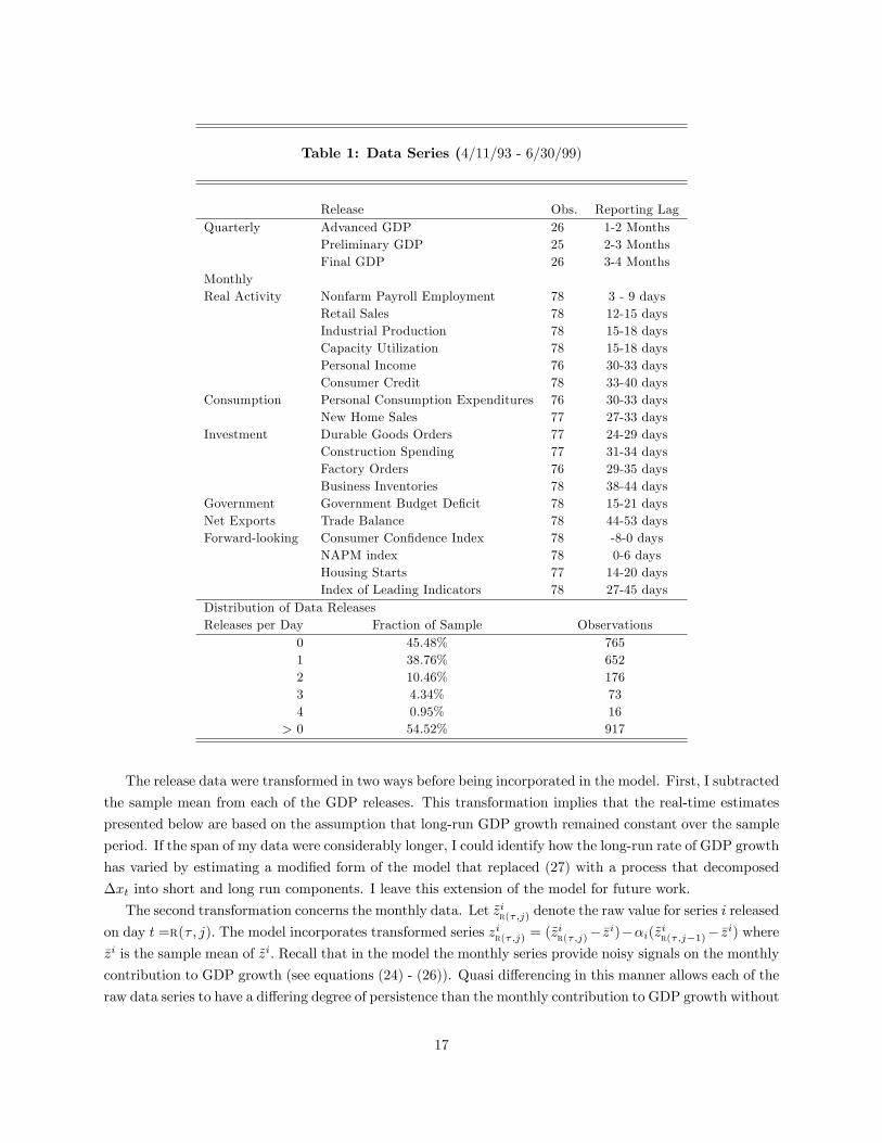
Table 1: Data Series (4/11/93 - 6/30/99)

Release Obs. Reporting LagQuarterly Advanced GDP 26 1-2 Months

Preliminary GDP 25 2-3 MonthsFinal GDP 26 3-4 Months

MonthlyReal Activity Nonfarm Payroll Employment 78 3 - 9 days

Retail Sales 78 12-15 daysIndustrial Production 78 15-18 daysCapacity Utilization 78 15-18 daysPersonal Income 76 30-33 daysConsumer Credit 78 33-40 days

Consumption Personal Consumption Expenditures 76 30-33 daysNew Home Sales 77 27-33 days

Investment Durable Goods Orders 77 24-29 daysConstruction Spending 77 31-34 daysFactory Orders 76 29-35 daysBusiness Inventories 78 38-44 days

Government Government Budget De�cit 78 15-21 daysNet Exports Trade Balance 78 44-53 daysForward-looking Consumer Con�dence Index 78 -8-0 days

NAPM index 78 0-6 daysHousing Starts 77 14-20 daysIndex of Leading Indicators 78 27-45 days

Distribution of Data ReleasesReleases per Day Fraction of Sample Observations

0 45.48% 7651 38.76% 6522 10.46% 1763 4.34% 734 0.95% 16

> 0 54.52% 917

The release data were transformed in two ways before being incorporated in the model. First, I subtracted

the sample mean from each of the GDP releases. This transformation implies that the real-time estimates

presented below are based on the assumption that long-run GDP growth remained constant over the sample

period. If the span of my data were considerably longer, I could identify how the long-run rate of GDP growth

has varied by estimating a modi�ed form of the model that replaced (27) with a process that decomposed

�xt into short and long run components. I leave this extension of the model for future work.

The second transformation concerns the monthly data. Let ~zir(�;j) denote the raw value for series i released

on day t =r(� ; j): The model incorporates transformed series zir(�;j) = (~zir(�;j)� �zi)��i(~zir(�;j�1)� �zi) where

�zi is the sample mean of ~zi: Recall that in the model the monthly series provide noisy signals on the monthly

contribution to GDP growth (see equations (24) - (26)). Quasi di¤erencing in this manner allows each of the

raw data series to have a di¤ering degree of persistence than the monthly contribution to GDP growth without

17

inducing serial correlation in the projection errors shown in (24) - (26). The degree of quasi-di¤erencing

depends on the �i parameters which are jointly estimated with the other model parameters.

4.2 Estimates and Diagnostics

The maximum likelihood estimates of the model are reported in Table 2. There are a total of 63 parameters in

the model and all are estimated with a great deal of precision. T-tests based on the asymptotic standard errors

(reported in parenthesis) show that all the coe¢ cient are signi�cant at the 1% level. Panel A of the table

shows the estimated parameters of the daily contribution process in (27). Notice that the reported estimates

and standard errors are multiplied by 25. With this scaling the reported values for the �i parameters

represent the coe¢ cients in the time-aggregated AR(6) process for �MxM(�;j) in a typical month (i.e. one

with 25 workdays). I shall examine the implications of these estimates for forecasting GDP below.

Panel B reports the estimated standard deviations of the di¤erence between the �advanced�and "�nal"

GDP releases, !a � yt � yt; and the di¤erence between the �preliminary�and ��nal�releases !p � ~yt � yt:According to equations (5) and (6) of the model, V(!a) = V(!p) +V(er(�)) so the standard deviation of !ashould be at least as great as that of !p: By contrast, the estimates in panel B imply that V(!a) < V(!p):7

This suggests that revisions the BEA made between releasing the �preliminary�and��nal�GDP data were

negatively correlated with the revision between the �advanced� and �preliminary� releases. It is hard to

understand how this could be a feature of an optimal revision process within the BEA. However, it is also

possible that the implied correlation arises simply by chance because the sample period only covers 25

quarters.

Estimates of the parameters linking the monthly data releases to GDP growth are reported in Panel C.

The �rst column shows that there is considerable variation across the 18 series in the estimates of �i: In all

cases the estimates of �i are statistically signi�cant indicating that the quasi-di¤erenced monthly releases

are more informative about GDP growth than the raw series. The �i estimates also imply that the temporal

impact of a change in growth varies across the di¤erent monthly series. For example, changes in GDP growth

will have a more persistent e¤ect on the Consumer Con�dence Index (�15 = 0:977) than on Nonfarm Payroll

Employment (�1 = 0:007): The �i estimates reported in the third column show that 12 of the 18 monthly

releases are pro-cyclical (i.e. positively correlated with contemporaneous GDP growth). Recall that all the

coe¢ cients are signi�cant at the 1% level so the �i estimates provide strong evidence that all the monthly

releases contain incremental information about current GDP growth beyond that contained in past GDP

data releases.

The standard method for assessing the adequacy of a model estimated by the Kalman Filter is to examine

the properties of the estimated �lter innovations, �t de�ned in (35a) above. If the model is correctly speci�ed,

all elements of the innovation vector �t should be uncorrelated with any elements of t�1; including past

innovations. To check this implication, Table 3 reports the autocorrelation coe¢ cients for the innovations

associated with each data release. For example, the estimated innovation associated with the ��nal�GDP

release for quarter � on day r(�), is �yr(�) � yr(�) � E[yr(�)jr(�)�1]: For the quarterly releases, the tableshows the correlation between �yr(�) and �

yr(��n) for n = 1 and 6: In the case of monthly release i, the

7To check robustness, I also estimated the model with the V(!a) = V(!p) + V(er(�)) restriction imposed. In this case theMLE of V(er(�)) is less than 0.0001.

18

Table 2: Model Estimates

A:Process for �xt�1 �2 �3 �4 �5 �6 �e

estimate�� �0:384 0.296 0.266 -0.289 -0.485 0.160 3.800standard error�� (0:004) (0.003) (0.003) (0.003) (0.003) (0.004) (0.010)

B: Quarterly Data ReleasesV(!i) sdt(!i)�

i = a Advanced GDP Growth 0.508 (0.177)p Preliminary GDP Growth 1.212 (0.312)

C: Monthly Data Releases�i sdt(�i)� �i sdt(�i)

� �i sdt(�i)�

i =1 Nonfarm Payroll Employment 0.007 (0.218) 0.656 (0.301) 0.932 (0.171)2 Retail Sales -0.047 (0.282) 0.285 (0.136) 0.381 (0.082)3 Industrial Production -0.028 (0.145) 0.189 (0.090) 0.229 (0.035)4 Capacity Utilization 0.924 (0.088) 0.125 (0.114) 0.382 (0.020)5 Personal Income -0.291 (0.219) 0.038 (0.126) 0.227 (0.040)6 Consumer Credit 0.389 (0.300) -0.160 (0.966) 2.961 (0.494)

7 Personal Cons. Expenditures -0.405 (0.206) 0.133 (0.074) 0.111 (0.029)8 New Home Sales 0.726 (0.170) -0.011 (0.171) 0.473 (0.071)

9 Durable Goods Orders -0.224 (0.258) 0.989 (0.753) 1.999 (0.413)10 Construction Spending 0.312 (0.197) -0.135 (0.233) 0.655 (0.123)11 Factory Orders -0.194 (0.288) 0.997 (0.489) -0.856 (0.306)12 Business Inventories 0.128 (0.277) -0.019 (0.061) 0.228 (0.032)

13 Government Budget De�cit -0.359 (0.418) -0.992 (1.423) 3.262 (0.508)

14 Trade Balance 0.819 (0.189) 0.361 (0.602) 1.585 (0.344)

15 Consumer Con�dence Index 0.977 (0.076) 0.208 (0.136) -0.482 (0.084)16 NAPM index 0.849 (0.115) -0.008 (0.047) 0.151 (0.024)17 Housing Starts 0.832 (0.175) 0.002 (0.026) 0.071 (0.014)18 Index of Leading Indicators 0.107 (0.240) 0.212 (0.077) 0.231 (0.033)

Notes: "*" and "**" indicate that the estimate or standard error is multiplied by 100 and 25 respectively.

innovation is �ir(�;j) � zir(�;j) � E[zir(�;j)jr(�;j)�1] and the table shows the correlation between �ir(�;j) and�ir(�;j�n) for n = 1 and 6. Under the BPQ(j) headings the table also reports p-values computed from the

Box-Pierce Q statistic for joint signi�cance of the correlations from lag 1 to j: Overall, there is little evidence

of serial correlation in the innovations. Exceptions arise only in the case of �preliminary�GDP at the six

quarter lag, and in the cases of consumer credit and business inventories at the six month lag.

Panel A of Table 4 compares model-based forecasts for ��nal�GDP against the provisional data releases.

Under the Data Revision columns I report the mean and mean squared error (M.S.E.) for the data revisions

associated with the �advanced� and �preliminary� data releases (i.e., yr(�)� yr(�) and yr(�) � ~yr(�)): Themean and M.S.E. for the di¤erent between ��nal�GDP, yr(�); and the estimates of E[yr(�)jdr(�)] where

19

Table 3: Model Diagnostics

Innovation Autocorrelations �1 BPQ(1) �6 BPQ (6)Quarterly Releases

Advanced GDP 0.058 (0.766) -0.061 (0.889)Preliminary GDP -0.364 (0.069) -0.034 (0.012)Final GDP 0.001 (0.996) -0.172 (0.729)

Monthly Releasesi = 1 Nonfarm Payroll Employment -0.023 (0.841) 0.051 (0.902)

2 Retail Sales 0.005 (0.966) -0.028 (0.789)3 Industrial Production 0.005 (0.963) 0.003 (0.981)4 Capacity Utilization -0.029 (0.800) 0.147 (0.885)5 Personal Income -0.069 (0.687) 0.057 (0.770)6 Consumer Credit -0.091 (0.422) 0.310 (0.040)

7 Personal Consumption Expenditures 0.122 (0.477) -0.021 (0.427)8 New Home Sales -0.219 (0.084) -0.056 (0.220)

9 Durable Goods Orders -0.094 (0.418) -0.121 (0.650)10 Construction Spending 0.064 (0.699) 0.131 (0.798)11 Factory Orders -0.161 (0.327) -0.113 (0.483)12 Business Inventories -0.068 (0.552) 0.339 (0.000)

13 Government Budget De�cit -0.091 (0.421) -0.137 (0.100)

14 Trade Balance -0.203 (0.077) 0.087 (0.578)

15 Consumer Con�dence Index 0.047 (0.678) -0.111 (0.624)16 NAPM index -0.067 (0.556) -0.017 (0.639)17 Housing Starts -0.160 (0.161) -0.127 (0.518)18 Index of Leading Indicators 0.021 (0.850) 0.043 (0.525)

Notes: �i denotes the sample autocorrelation at lag i: p-values are calculated forthe null hypothesis of �i = 0.

dr(�) denotes the date of the day of either the �advanced�and �preliminary�release (i.e., ry(�) or r~y(�))

are reported under the Model columns. Note that the provisional data are part of the information set dr(�)used to compute the model-based forecasts. If yr(�) and ~yr(�) are close to the best forecasts of ��nal�GDP

on days ry(�) and r~y(�); there should be little di¤erence between the data revisions and the estimated

forecast errors, yr(�) � E[yr(�)jdr(�)].8 The table shows that the mean and M.S.E. of revision errors based

8The model does not impose the assumption that the provisional data are equal to the best forecast of ��nal�GDP on daydr(�): Rather, equation (34a) of the Kalman Filter implies that the model forecasts for ��nal�GDP on these days are given by

E[yr(�)jdr(�)] = E[yr(�)jdr(�)�1] + Kydr(�)��yr(�) � E[�yr(�)jdr(�)�1]

�+ K{

dr(�)

�{r(�) � E[{r(�)jdr(�)�1]

�where �yr(�) =

�yr(�); ~yr(�)

and {r(�) denotes the vector of other data releases on dr(�). Kydr(�) and K

{dr(�)

are elements of the

Kalman Gain matrix on release days. Inspection of this equation reveals that E[yr(�)jdr(�)] = �yr(�) if Kydr(�) = 1 and K{dr(�)

is a vector of zeros. These conditions cannot be exactly satis�ed when there is any noise in (5) and (6), but they could holdapproximately if the noise variance is small relative the variance of other shocks. Under these circumstances, the provisional

20

on the �preliminary� data releases are comparable to those based on the model forecasts. In the case of

the �advance�releases, by contrast, the mean revision error is roughly two-and-a-half times the size of the

forecast error. This �nding suggests that the �advanced�releases contain some �noise�and do not represent

the best forecasts for ��nal�GDP that can be computed using publicly available data. It is also consistent

with the regression �ndings reported by Dynan and Elmendorf (2001).

Table 4: Forecast Comparisons

A: Data Revision ModelMean M.S.E. Mean M.S.E.

Advanced 0.246 (0.446) 0.090 (0.441)Preliminary 0.038 (0.067) 0.040 (0.066)Combined 0.142 (0.257) 0.065 (0.254)

B: M.M.S. ModelMean M.S.E. Mean M.S.E

In-sampleAdvanced 0.729 (1.310) 0.190 (1.407)Preliminary 0.160 (0.249) 0.096 (0.418)Final 0.042 (0.062) 0.080 (0.395)Combined 0.310 (0.540) 0.122 (0.740)Out-of-sampleAdvanced 0.985 (1.464) 0.380 (1.500)Preliminary 0.046 (0.178) 0.178 (0.801)Final -0.015 (0.057) 0.099 (0.208)Combined 0.338 (0.566) 0.219 (0.836)

Panel B of Table 4 compares the forecasting performance of the model against the survey responses

collected by MMS. On the Friday before each scheduled data release, MMS surveys approximately forty

professional money managers on their estimate for the upcoming release. Panel B compares the median

estimate from the surveys against the real-time estimate of GDP growth implied by the model on survey days.

For example, in the �rst row under the MMS columns I report the mean and M.S.E. for the di¤erence between

yr(�); and the median response from the survey conducted on the last Friday before the �advanced�GDP

release on day s(�). The mean and M.S.E of the di¤erence between yr(�) and the estimate of E[yr(�)js(�)]derived from the model are reported under the Model columns. As above, all the survey and model estimates

are compared against the value for the ��nal�GDP release. This means that the forecasting horizon, (i.e.

the di¤erence between r(�) and s(�)) falls from approximately 11 weeks in the �rst row, to �ve weeks in

the second, and less than one week in the third. The fourth row reports the mean and M.S.E. at all three

horizons.

The upper portion of Panel B compares the survey responses against model-based forecasts computed

from parameter estimates reported in Table 2. These estimates are derived from the full data sample and

data could closely approximate the model�s forecasts for ��nal�GDP (i.e., E[yr(�)jdr(�)] ' �yr(�)):

21

so contain information that was not available to the money mangers at the time they were surveyed. The

lower portion of Panel B reports on a pseudo out-of-sample comparison. Here the model-based forecasts

are computed from model estimates obtained from the �rst half of the sample (4/11/93 - 3/31/96). These

estimates are then used to compute model-based forecasts of ��nal�GDP on the survey days during the

second half of the sample (4/01/96 - 6/30/99). The table compares the mean and M.S.E. of these out-of-

sample forecasts against the survey responses during this latter period.

The table shows that both the mean and M.S.E. associated with both the survey and model forecasts fall

with the forecasting horizon. In the case of the in-sample statistics, the median survey response provides a

superior forecast than the model in terms of mean and M.S.E at short horizons. Both the mean and M.S.E.

are smaller for survey responses than the model forecasts in the third row. Moving up a row, the evidence

is ambiguous. The model produces a smaller mean but larger M.S.E. than the median survey. In the �rst

row, the balance of the evidence favors the model; the M.S.E. is slightly higher but the mean is much lower

than the survey estimates. This general pattern in repeated in the out-of-sample statistics. The strongest

support for the model again comes from a comparison of the survey and model forecasts conducted one week

before the �advanced�release. In this case the mean forecast error from the model is approximately 60 per

smaller than the mean survey error. Over shorter forecasting horizons, the survey measures dominate the

model-based forecasts.

Overall, these forecast comparisons provide rather strong support for the model. It is clear that the

in-sample comparisons use model estimates based in part on information that was not available the money

managers at the time. But it is much less clear whether this puts the managers at a signi�cant informational

disadvantage. Remember that the money managers had access to private information and other contempo-

raneous data that is absent from the model. Moreover, we are comparing a model-based forecast against the

median forecast from a forty manager survey. In the out-of-sample comparisons, the informational advantage

clearly lies with the managers. Here the model forecast are based on a true subset of the information available

to managers so the median forecast from a forty manager survey should outperform the model. This is what

we see when the forecasting horizon is less than �ve weeks. At longer horizons, the use of private information

imparts less of a forecasting advantage to money managers.9 In fact, the results suggest that as we move

the forecasting day back towards then end of quarter � ; both the in and out-of-sample model-based forecasts

outperform the surveys. When the forecasting day is pushed all the way back to the end of the quarter, the

model-based forecast gives us the real-time estimates of GDP growth. Thus, the results in panel B indicate

that real-time estimates derived from the model should be at least comparable to private forecasts based on

much richer information sets.

9This advantage might be further reduced if each of the model forecasts were computed using parameter estimates thatutilized all the data available on the survey date rather than a single set of estimates using data from the �rst half of thesample. A full-blown real-time forecasting exercise of this kind would be computationally demanding because the model wouldhave to be repeatedly estimated, but it should also give superior model-based forecasts. For this reason, the out-of-sampleexercise undertaken here probably understates the true real-time forecasting potential of the model.

22

5 Analysis

This section examines the model estimates. First, I consider the relation between the real-time estimates

and the ��nal�GDP releases. Next, I compare alternative real-time estimates for the level of GDP and

examine the forecasting power of the model. Finally, I study how the monthly releases are related to changes

in GDP at a monthly frequency.

5.1 Real-time Estimates over the Reporting Lag

Figure 2 allows us to examine how the real-time estimates of GDP growth change over the reporting lag.

The green line plots the ��nal�GDP growth for quarter � released on day ry(�). The blue line plots the

real-time estimates of the GDP growth last month �qxq(�)jt where q(�) < t � ry(�) for each quarter. Thevertical dashed portion represent the discontinuity in the series at the end of each quarter (i.e. on day

q(�)):10 Several features of the �gure stand out. First, the real-time estimates vary considerably in the days

immediately after the end of the quarter. For example, at the end of 1994, the real-time estimates of GDP

growth in the forth quarter change from approximately 1.25% to 2.25% and then to 1.5% in the space of a

few days. Second, in many cases there is very little di¤erence between the value for ��nal�GDP and the

real-time estimate immediately prior to the release (i.e., yr(�) ' �qxq(�)jr(�)�1): In these cases, the ��nal�release contains no new information about GDP growth that was not already inferred from earlier data

releases. In cases where the ��nal� release contains signi�cant new information, the blue plot �jumps� to

meet the green plot on the release day.

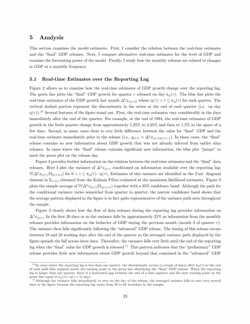
Figure 3 provides further information on the relation between the real-time estimates and the ��nal�data

releases. Here I plot the variance of �qxq(�) conditioned on information available over the reporting lag;

V(�qxq(�)jq(�)+i) for 0 < i � ry(�)�q(�): Estimates of this variance are identi�ed as the 2�nd. diagonalelement in St+1jt obtained from the Kalman Filter evaluated at the maximum likelihood estimates. Figure 3

plots the sample average of V(�qxq(�)jq(�)+i) together with a 95% con�dence band. Although the path forthe conditional variance varies somewhat from quarter to quarter, the narrow con�dence band shows that

the average pattern displayed in the �gure is in fact quite representative of the variance path seen throughout

the sample.

Figure 3 clearly shows how the �ow of data releases during the reporting lag provides information on

�qxq(�): In the �rst 20 days or so the variance falls by approximately 25% as information from the monthly

releases provides information on the behavior of GDP during the previous month (month 3 of quarter �):

The variance then falls signi�cantly following the �advanced�GDP release. The timing of this release occurs

between 19 and 23 working days after the end of the quarter so the averaged variance path displayed by the

�gure spreads the fall across these days. Thereafter, the variance falls very little until the end of the reporting

lag when the ��nal�value for GDP growth is released.11 This pattern indicates that the �preliminary�GDP

release provides little new information about GDP growth beyond that contained in the �advanced�GDP

10 In cases where the reporting lag is less than one quarter, the discontinuity occurs (a couple of days) after ry(�) so the endof each solid blue segment meets the turning point in the green line identifying the ��nal�GDP release. When the reportinglag is longer than one quarter, there is a horizontal gap between the end of a blue segment and the next turning point on thegreen line equal to ry(�)�q(� + 1) days.11Although the variance falls immediately to zero on the day of the release, the averaged variance falls to zero over several

days in the �gure because the reporting lag varies from 58 to 65 workdays in the sample.

23

Figure 2: Real-time esimtates of quarterly GDP growth �qxq(�)jt where q(�) < t � ry(�) (blueline), and ��nal�releases for GDP growth (green line).

release and the monthly data. The �gure also shows that most of the uncertainty concerning GDP growth

in the last quarter is resolved well before the day when the ��nal�data is released.

5.2 Real-Time Estimates of GDP and GDP Growth

Figure 4 compares the real-time estimates of log GDP against the values implied by the ��nal�GDP growth

releases. The red line plots the values of xq(�)jt computed from (43):

xq(�)jt = E[xtjt] +q(�)�tXh=1

E[�xt+hjt]: (44)

Recall that xq(�) represents log GDP for quarter � ; so xq(�)jt includes forecasts for �xt+h over the remaining

days in the quarter when t < q(�): To assess the importance of the forecast terms, Figure 4 also plots

E[xtjt] in blue. This series represents a naive real-time estimate of GDP since it assumes E[�xt+hjt] = 0for 1 � h �q(�) � t: The dashed green line in the �gure plots the cumulant of the ��nal�GDP releasesP�

i=1 yr(i) with a lead 60 days. This plot represents an ex post estimate of log GDP based on the ��nal�

24

Figure 3: The solid line is the sample average of V(�qxq(�)jq(�)+i) for 0 < i � ry(�)�q(�) , andthe dashed lines denote the 95% con�dent band. The horizontal axis marks the the number of daysi past the end of quarter q(�):

data releases. The vertical steps identify the values for ��nal�GDP growth 60 days before the actual release

day.

Figure 4 displays three notable features. First, both sets the real-time estimates display a much greater

degree of volatility than the cumulant series. This volatility re�ects how inferences about current GDP

change as information arrives in the form of monthly data releases during the current quarter and GDP

releases referring to growth in the previous quarter. The second noteworthy feature concerns the relation

between the real-time estimates. The vertical di¤erence between the red and blue plots represents the

contribution of the �xt+h forecasts to xq(�)jt: As the �gure shows, these forecasts contributed signi�cantly

to the real-time estimates in 1996 and 1997, pushing the real-time estimates of xq(�) well below the value

for E[xtjt]. The third noteworthy feature of the �gure concerns the vertical gap between the red and greenplots. This represents the di¤erence between the real-time estimates and an ex post estimate of log GDP

based on the ��nal�GDP releases. This gap should be insigni�cant if the current level of GDP could be

precisely inferred from contemporaneously available data releases. Figure 3 shows this to be the case during

the third and forth quarters of 1995. During many other periods, the real-time estimates were much less

precise.

25

Figure 4: Real-time estimates of log GDP xq(�)jt (red line), E[xtjt] (blue line) and cumulant of��nal�GDP releases (green dashed line).

5.3 Forecasting GDP Growth

The model estimates in Table 2 show that all of the �i coe¢ cients in the daily growth process are statistically

signi�cant. I now examine their implications for forecasting GDP growth. Consider the di¤erence between

the real time estimates of xt+m and xt+n based on information available on days t +m and t + n; where

m > n :

xt+mjt+m � xt+njt+n =t+mX

h=t+n+1

E [�xhjt] +�xt+mjt+m � xt+mjt

���xt+njt+n � xt+njt

�: (49)

This equation decomposes the di¤erence in real-time estimates of xt into forecasts for �xt over the forecast

horizon between t+n and t+m; the revision in the estimates of xt+m between t and t+m and xt+n between

t and t+ n:

Since both revision terms are uncorrelated with elements of t, we can use (49) to examine how the

predictability of �xt implied by the model estimates translates into predictability for changes in xtjt. In

26

particular, after multiplying both sides of (49) by xt+mjt+m � xt+njt+n and taking expectations, we obtain

R2 (m;n) =Pt+m

h=t+n+1 CV�E [�xhjt] ; xt+mjt+m � xt+njt+n

�V�xt+mjt+m � xt+njt+n

� :

This statistic measures the contribution of �xt forecasts to the variance of xt+mjt+m � xt+njt+n: If most ofthe volatility in xt+mjt+m � xt+njt+n is due to the arrival of new information between t and t + m ( i.e.,

via the revision terms in (49)), the R2 (m;n) statistic should be close to zero. Alternatively, if the the dailygrowth process is highly forecastable, much less of the volatility in xt+mjt+m � xt+njt+n will be attributableto news and the R2 (m;n) statistic will be positive.

Table 5: Forecasting Real-time GDP

m R2(m;n) (sdt.)Monthly (n = m� 20)

20 0.196 (0.015)40 0.186 (0.014)60 0.180 (0.013)80 0.163 (0.013)100 0.138 (0.012)120 0.125 (0.011)140 0.097 (0.010)160 0.061 (0.007)180 0.032 (0.006)200 0.035 (0.006)220 0.027 (0.006)240 0.005 (0.006)

Quarterly: (n = m� 60)60 0.144 (0.008)120 0.079 (0.006)180 0.031 (0.003)240 0.006 (0.002)

The table reports estimates of R2(m;m � 20)computed as the slope coe¢ cient �m fromthe regression

Pt+mh=t+m�19E [�xhjt] =

�m�xt+mjt+m � xt+m�20jt+m�20

�+ �t+m computed

in daily data from the maximum likelihood estimates ofxt+mjt+m�xt+m�20jt+m�20 and E [�xhjt] : OLS standarderrors are reported in the right hand column.

Table 5 reports estimates for R2(m;n) for various forecasting horizons. The estimates are computed asthe slope coe¢ cient in the regression of

Pt+mh=t+n+1 E [�xhjt] on xt+mjt+m � xt+njt+n in daily data. The

table also reports OLS standard errors in parenthesis.12 The upper panel shows how predictable the monthly

12These statistics only approximate to the true standard errors for two reasons. First, the regressor is computed from themaximum likelihood estimates and so contians some samplying error. Second, there is no correction for MA process inducedby the overlapping forecast horizons in the regression residuals.

27

changes in the real-time estimates of xt are for horizons m of 20 to 240 days. The estimated process for �xtimplies a reasonable high degree of predictability: the R2 estimates fall from approximately 20 to 10 per

cent as horizon rises from 20 to 140 workdays. Estimates of R2(m;n) for quarterly changes in the real-timeestimates are reported in the lower panel of the table. These are somewhat smaller, but again clearly indicate

the presence of some predictability.

The results in Table 5 related to the change in the real-time estimates of xt rather than GDP growth.

Recall from (43) that the real-time estimate of log GDP on day t in quarter � is xq(�t)jt = E[xtjt] +Pq(�t)h=t+1 E[�xhjt]; so the growth in quarterly GDP between quarters � and � + 1 based on the real-time

estimates available at t+m and t+ n (where t+ n < q(�) < t+m < q(� + 1)) is

xq(�+1)jt+m � xq(�)jt+n =�xt+mjt+m � xt+njt+n

�+

q(�+1)Xh=t+m+1

E[�xhjt+m]�q(�)X

h=t+n+1

E[�xhjt+n]: (50)

This equation shows that changes in the real-time estimates of xt are only one component of the estimated

quarterly growth in GDP. Moreover, since the second and third terms on the right hand side of (50) will

generally be correlated with the �rst term, the results in Table 5 may an unreliable guide to the predictability

of GDP growth.

Figure 5: Real-time estimates of the quarterly growth in GDP, xq(�+1)jt+60�xq(�)jt (red line), andex ante forecasts, E[xq(�+1) � xq(�)jt] (blue line).

28

We can examine the predictability of GDP growth by combining (49) and (50) to give

xq(�+1)jt+m � xq(�)jt+n = E[xq(�+1) � xq(�)+1jt] + &t+m;

where &t+m is an error term that depends on news that arrives between t and t +m: This equation shows

that GDP growth should be predictable in the model because the process for �xt implies that E[xq(�+1) �xq(�)+1jt] changes over the sample. Figure 5 plots the estimates of E[xq(�+1)�xq(�)+1jt] and xq(�+1)jt+m�xq(�)jt+n for m = 60 and n = 0: Clearly, news contributes signi�cantly to the volatility of GDP growth

since the E[xq(�+1) � xq(�)+1jt] series is much less volatile than xq(�+1)jt+m � xq(�)jt+n: In fact, only 6per cent of the variance in xq(�+1)jt+m � xq(�)jt+n can be attributable to E[xq(�+1) � xq(�)+1jt] over thesample. While this implies a rather modest degree of predictability, close inspection of Figure 5 suggests that

predicting the future direction of GDP growth may be a little more successful. Indeed, the model estimates

of E[xq(�+1) � xq(�)+1jt] correctly predict the direction of GDP growth 59 per cent of the time.For perspective on these forecasting results, I also estimated an AR(2) model for quarterly GDP growth

using the sequence of ��nal�GDP releases. This model provides a simple time series forecast for GDP growth

(approximately) one quarter ahead, based on the two most recent releases. In contrast to the results presented

above, estimates of the AR(2) model do not indicate that quarterly GDP growth is at all predictable: The

coe¢ cients are small and statistically insigni�cant and the R2 statistic is only 3 per cent. These results are

hardly surprising. Remember that the sample mean was removed from all the GDP growth releases so we are

attempting to forecast future deviations in GDP growth. Figure 2 shows that these deviations display little

serial correlation. Thus, it is not surprising that the history of GDP releases has little forecasting power.

These observations also point to the signi�cance of the forecasting results displayed in Table 5 and Figure 5.

In particular, they show that monthly data releases contain information that is useful for both estimating

the current state of the GDP and for forecasting its future path. This aspect of the model ties in with recent

research that harnesses the information in a large number of indicators for forecasting (see, for example,

Stock and Watson 2002). The results from these studies suggest that the real-time forecasting performance

of this model may be further enhanced by addition of other macroeconomic and �nancial indicators.

5.4 Monthly Estimates of GDP Growth

One of the unique features of the model is its ability to provide us with high frequency estimates of log GDP

and GDP growth. I now examine how the monthly data releases relate to the changing real-time estimates

of log GDP. My aim is to provide a simply description of the complex inference problem solved by the model

regarding the current state of GDP.

Let t and t+20be workdays in quarters �0 and �1 with t � q(�0) and t+20 � q(�1): (Note that �0 and�1 can refer to the same quarter.) I consider two regression models. The �rst relates the monthly change in

the real-time estimates of log GDP to all 18 monthly releases:

xq(�1)jt+20 � xq(�0)jt =18Xi=1

ai(rit+20 � rit) + �t+20; (51)

where rit denotes the last value released for series i on day t: Thus, the value of rit remains that same from

29

day to day unless t is the day on which a data release for series i takes place. This means that rit+20 � ritidenti�es the change in the latest value for series i released during the 20 workdays ending on t + 20: The

second model relates the change in the real-time estimates to each monthly release separately:

xq(�1)jt+20 � xq(�0)jt = bi(rit+20 � rit) + �t+20; (52)

for i = 1; 2; ::18: Notice that the regressors in both models are available on a daily bases. Estimates of

the ai and bi coe¢ cients therefore summarize how the complex inference imbedded in the model relate to

observable changes in the information set comprised of monthly data releases.

Table 6: Monthly Indicator Estimates

Data Release ai std(ai) bi std(bi) R2

i =1 Nonfarm Payroll Employment 0.224� (0.033) 0.330� (0.050) 0.2332 Retail Sales 0.520� (0.074) 0.838� (0.099) 0.1863 Industrial Production 0.745� (0.116) 1.047� (0.142) 0.2334 Capacity Utilization -0.006 (0.034) 0.066 (0.057) 0.0105 Personal Income -0.110 (0.132) 0.163 (0.224) 0.0036 Consumer Credit 0.001 (0.012) -0.002 (0.019) 0.000

7 Personal Consumption Expenditures 0.377� (0.182) 0.603� (0.277) 0.0338 New Home Sales 0.016 (0.069) 0.181� (0.088) 0.039

9 Durable Goods Orders 0.013 (0.021) 0.064� (0.027) 0.03010 Construction Spending -0.050 (0.051) -0.102 (0.060) 0.01511 Factory Orders 0.097� (0.038) 0.160� (0.043) 0.06612 Business Inventories -0.013 (0.152) 0.289 (0.247) 0.008

13 Government Budget De�cit -0.008 (0.011) -0.017 (0.016) 0.005

14 Trade Balance -0.071� (0.021) -0.068� (0.030) 0.042

15 Consumer Con�dence Index 0.068� (0.028) 0.060 (0.037) 0.02116 NAPM index -0.001 (0.145) 0.514� (0.216) 0.04617 Housing Starts -1.330� (0.421) 0.705 (0.546) 0.01218 Index of Leading Indicators 0.164 (0.179) 0.476� (0.199) 0.038

Notes: The table reports the OLS estimates of ai and bi from equations (51) and (52). Both equations areestimated at the daily frequency, and the standard errors are corrected for the MA(19) process induced bythe overlapping data. The right hand column reports the R2 statistic from estimating equation (52). A ���denotes signi�cance at the 5 per cent level.

Table 6 reports the estimates of equations (51) and (52). The left hand columns show that the aiestimates are statistically signi�cant for data on nonfarm payroll, retail sales, industrial production, personal

consumption, factory orders, the trade balance, the index of consumer con�dence and housing starts. Each of

these data releases provides signi�cant incremental information about the change in the real-time estimates.

The 18 monthly releases account for approximately 57 per cent of the variance in xq(�1)jt+20 � xq(�0)jt: This

30

means that more than 40 per cent of the variation in the real-time estimates is not captured by the simple

linear speci�cation. The right hand columns report the results from estimating equation (52). The most

noteworthy aspects of these estimates can be seen for i = 1; 2; and 3: Changes in both nonfarm payroll

and retail sales appear strongly linked to changes in the real-time estimates. Based on the R2 statistics

(in the right hand column), these variables account for 23 and 19 per cent of the variance in the real-time

estimates. The results for i = 3 provide some justi�cation for the frequent use of industrial production as a

monthly proxy for GDP growth. The estimate for b3 indicates the real-time estimates of log GDP change

approximately one-for-one with change in industrial production between releases. Notice, however, that the

R2 statistic is only 0.233. Industrial production does not account for most of the variance in the real-time

estimates.

6 Conclusion

In this paper I have presented a method for estimating the current state of the economy on a continual basis

using the �ow of information from a wide range of macroeconomic data releases. These real-time estimates

were computed from an econometric model that allows for variable reporting lags, temporal aggregation,

and other complications that characterize the daily �ow of macroeconomic information. The model can be

applied to �nd real-time estimates of GDP, in�ation, unemployment or any other macroeconomic variable

of interest.

In this paper I focused on the problem of estimating GDP in real time. This application of the estimation

procedure should be of particular interest to policymakers concerned with the lack of timely information about

economy-wide real activity. The real-time estimates I calculate have several noteworthy features: First, the

estimates of log GDP display a good deal of high-frequency volatility. This volatility re�ects how inferences

about current GDP change as information arrives in the form of monthly data releases during the quarter.

Second, the gaps between the real-time estimates and ex post GDP data are on occasion both persistent

and signi�cant. These �ndings suggest that the ex post data should not be viewed as a close approximation

to what was known at the time. Third, the model estimates reveal that the monthly data releases contain

information that is useful for forecasting its future path of GDP. Finally, my comparison of the real-time

estimates with the monthly data series shows that standard proxies for real actively at the monthly frequency

capture only a fraction of the variance in the real-time estimates.

These �ndings give but a �avor of the uses to which real-time estimates could be put. One obvious topic

for the future concerns the ability of the real-time estimates and forecasts to identify turning points in the

business cycle. This issue could be readily addressed if the model were re-estimated over a much longer

time-span than was undertaken here. The use of real-time estimates may also bring new perspective to

the link between asset prices and macroeconomic fundamentals. Evans and Lyons (2004a) use the methods

described here to construct real-time estimates for GDP, in�ation, and money supplies for the U.S. and

Germany. With the aid of these estimates, they then show that foreign exchange transactions contain

signi�cant information about the future path of fundamentals. Since transaction �ows also exert a very

strong in�uence on exchange rate dynamics in the short run, this �nding points to a much stronger link

between fundamentals and exchange rates than pervious research has uncovered. It remains to be seen

whether the use of real-time estimates will similarly illuminate the links between macro fundamentals and

31

other asset prices.

32

References

Andersen, T. G., T. Bollerslev, F. Diebold and C. Vega (2003), � Mirco E¤ect of Macro Announcements:

Real-Time Price Discovery in Foreign Exchange�, American Economic Review, 93(1), March, pp. 38-

62.

Balduzzi, P., E. J. Elton and T. C. Green (2001), � Economic News and Bond Prices: Evidence from the

U.S. Treasury Market�, Journal of Financial and Quantitative Analysis, 36(4), December, pp. 523-43.

Carson, C. S. (1987), �GNP: An Overview of Source Data and Estimation Methods�, Survey of Current

Business, 67(7) July, pp.103-26.

Chow, G. and A. Lin (1971), �Best Linear Unbiased Interpolation, Distribution, and Extrapolation of Time

Series by Related Time Series�, Review of Economics and Statistics, 53, pp.372-75.

Clarida, R., J. Kitchen and R. Monaco (2002), �Real-Time Forecasting in Practice: A Description of the U.S.

Treasury�s Real-time GDP Forecasting System�, mimeo, O¢ ce of Economic Policy, U.S. Department

of the Treasury.

Croushore, D. and T. Stark (1999), �A Real-Time Data Set for Macroeconomists�, Federal Reserve Bank

of Philadelphia, working paper 99-4, June.

Croushore, D. and T. Stark (2001), ��A Real-Time Data Set for Macroeconomists�, Journal of Econometrics

105, November, pp. 111-130.

Dynan, K. E. and D. W. Elmendorf (2001), �Do Provisional Estimates of Output Miss Economic Turning

Points?�, mimeo, Federal Reserve Board.

Evans, M.D.D. and R. K. Lyons (2004a), �A New Micro Model of Exchange Rate Dynamics�, NBER

working paper No. 10379, March.

Evans, M.D.D. and R. K. Lyons (2004b), �Do Currency Transaction Flows Forecast Fundamentals?�,

mimeo, March, (available at http://www.georgetown.edu /faculty/evansm1 /wpapers_�les /�owsnber.pdf).

Faust, J., Rogers, J. and J. Wright (2000), �New and Noise in G-7 GDP Announcements�, Federal Reserve

Board International Finance Discussion Paper No. 2000-690.

Hamilton, J. D. (1994), Time Series Analysis, Princeton University Press, Princeton, New Jersey.

Harvey, A. C. (1989), Forecasting Structural Time Series Models and the Kalman Filter, Cambridge Uni-

versity Press, Cambridge, U.K.

Lui, H. and S. G. Hall (2000), � Creating High Frequency National Accounts with State Space Modelling:

A Monte Carlo Experiment�, mimeo, Imperial College, London, U.K.

Mariano, R. and Y. Murasawa (2003), �A New Coincident Index of Business Cycles Based on Monthly and

Quarterly Series�, Journal of Applied Econometrics , 18, pp.427-443.

33

Mankiw, N. and M. Shapiro (1986), �News or Noise: An Analysis of GNP Revisions�, Survey of Current

Business, 66(5), pp. 20-25.

Orphanides, A. (2001), �Monetary Rules Based on Real-Time Data�, American Economic Review.

Robertson, J. and E. Tallman (1999), �Vector Autoregressions: Forecasting and Reality�, Federal Reserve

Bank of Atlanta Economic Review, QI.

Seskin, E. P. and R. P. Parker (1998), �A Guide to the NIPA�s�, Survey of Current Business, 78(3), March,

pp. 26-68.

Stock, J. and M. Watson (2002) �Macroeconomic Forecasting Using Di¤usion Indexes�, Journal of Business

and Economic Statistics, 20(2), pp. 147-162,

Urich, T. J., and P. Watchel (1984), �The E¤ects of In�ation and Money Supple Announcements on Interest

Rates�, Journal of Finance, 39(4), September, pp. 1177-88.

34