[Under review at Marketing Science. Please do not quote or distribute. All comments welcome.]

When Random Assignment Is Not Enough:

Accounting for Item Selectivity in Experimental Research

Yuanping Ying*

Linda Court Salisbury*

Fred M. Feinberg*

Yuanping Ying (yingyp@utdallas.edu; Tel: (972)883-4737) is Assistant Professor of Marketing at the University of Texas at Dallas, 800 West Campbell Rd., SM32, Richardson, Texas 75080-3021. Linda Court Salisbury (salisbli@bc.edu; Tel: 617-552-3142; Fax: 617-552-6677) is Associate Professor of Marketing at the Carroll School of Management, Boston College, 140 Commonwealth Avenue, Chestnut Hill, MA 02467. Fred M. Feinberg (feinf@umich.edu; Tel: 734-764-4711; Fax: 734-936-0279) is Handleman Professor of Marketing, Ross School of Business, and Professor of Statistics, University of Michigan, 701 Tappan Street, Ann Arbor, MI, 48109-1234. The authors wish to thank Greg Allenby, Christie Brown, Clint Cummins, Terry Elrod, Gabor Kezdi, and Carolyn Yoon for their assistance and suggestions.  

1  

When Random Assignment Is Not Enough:

Accounting for Item Selectivity in Experimental Research

Abstract

A common goal in marketing research is to understand how one evaluates products that have

been filtered through some type of screening or selection process. Typical examples include post-choice

satisfaction ratings, certain free recall tasks, or the development of consideration sets followed by brand

choice. In such situations, behavior is contingent not only on the alternatives being evaluated, but the

choice context in which they have become available, creating differing degrees of selectivity.

In this paper, we consider situations in which a polytomous selection process limits which items

offer up subsequent information. We propose that not flexibly modeling the correlation between choice

and evaluation across conditions can lead to systematic, erroneous interpretations of covariate effects on

evaluation. We illustrate this by analyzing two experiments in which subjects choose among, and then

evaluate, a frequently-purchased consumer good, as well as data first examined by Ratner, Kahn and

Kahneman (1999). Results indicate not only strong selectivity effects, but that traditional specifications of

the choice process – presuming the degree of selectivity is invariant across choice contexts – can lead to

markedly different interpretations of variable effects. Our findings show that the size and composition of

a choice set affects the degree of correlation between choice and evaluation, and further suggest that

foregone alternatives can play a disproportionate role in selectivity. Moreover, failing to account for

selectivity across experimental conditions, even in well-designed experimental settings, can lead to

inaccurate substantive inferences about consumers’ choice processes.

Keywords: Choice Models, Consumer Behavior, Decision-Making, Econometric Models, Sample

Selection, Heckman Model, Markov chain Monte Carlo, Hierarchical Bayes

2  

INTRODUCTION

Selectivity artifacts are common problems in academic disciplines characterized by field research

– labor economics and sociology, for example – in which it is not often possible to guarantee a random

sample of the population of interest. In these fields, researchers have come to rely on statistical models

designed to correct for respondents’ providing feedback only on items that have been selected in some

manner. There is a long history of such models in economics, dating back to the classic papers of Tobin

(1958) and Heckman (1976, 1979), and they are becoming such fundamental tools that full scale reviews

have appeared in cognate disciplines (e.g., Berk 1983, Winship and Mare 1992, Vella 1998), as well as

economics proper (Heckman 1990, Heckman et al. 1998, Puhani 2000).

More recently, there has been a surge of interest in the topic among quantitative researchers in

marketing, starting with the pioneering work of Krishnamurthi and Raj (1988) and Jedidi, Mela, and

Gupta (1999) on jointly modeling brand choice and purchase incidence, and presently encompassing a

wide variety of data settings, including models: accounting for panel attrition (Danaher 2002); assessing

the long-run effects of promotion using RFM variables (Anderson and Simester 2004); of duration and

customer profitability, observed only for customers that are acquired (Reinartz, Thomas, and Kumar

2005); of customers’ online banking decisions conditional on having signed up and logged in (Lambrecht,

Seim, and Tucker 2011); allowing for correlated errors in incidence and strength of online product

opinions (Moe and Schweidel 2012; Ying et al. 2006); serving as robustness checks against those

providing particular information, like word-of-mouth (Yang et al. 2012); to interrelate content creation

and purchase decisions (as well as their utilities; Albuquerque et al. 2012); and culminating in Wachtel

and Otter’s (2013) comprehensive framework to account for multiple waves of selectivity (e.g., scoring

and targeting) enacted deliberately by marketers. Notably, the vast majority of such work in empirical

modeling has had to contend with selectivity in field data, over which investigators have little, if any,

direct control.

By contrast, corresponding problems in experimental consumer research are often tacitly assumed

to be nonexistent, or at worst minor. Because they often have the luxury of randomly assigning subjects to

3  

experimental conditions, laboratory researchers have been considered largely exempt from the need to be

concerned with selectivity. This was noted in an influential paper by Degeratu, Rangaswamy, and Wu

(2000), who suggested that, to study internet purchase patterns, one would ideally need to conduct a

randomized experiment in which some people are assigned to shop online and some offline. Specifically,

they contrast the controlled experimental settings typical to behavioral researchers with that encountered

in field data. Random assignment in experimental settings is taken as sufficient to control for selectivity

artifacts that can arise, for example, when people provide product ratings only for items they have chosen.

While in many cases it does, in others it does not.

In this paper, we show that selectivity artifacts can arise even in well-designed experimental settings,

and should be both measured and carefully modeled in order to obtain appropriate substantive inferences.

Specifically, selection or screening processes are frequently a critical, if unheralded, part of experimental

research in marketing and decision theory. Consider, for example, the following situations:

A consumer chooses among alternatives, then indicates satisfaction with his/her choice (Ratner,

Kahn, and Kahneman 1999; Zhang and Fitzsimons 1999; Shiv and Huber 2000; Diehl and Poynor

2010; Litt and Tormala 2010).

A consumer chooses among alternatives, then makes a follow-up choice (Iyengar and Lepper

2000), or decides whether to switch to another brand (Read and Loewenstein 1995; Fitzsimons

2000); or a consumer chooses what product information to examine, then chooses a brand (Braun

1999);

A consumer develops a consideration set then makes a final choice (Haübl and Trifts 2000;

Chakravarti and Janiszewki 2003; Van Nierop et al. 2010); or a consumer makes a sequence of

choices reducing the set of alternatives by stages until only one remains (Tversky 1972, Levin et

al. 1991, 1998).

These are commonly encountered experimental situations in which selectivity artifacts may be

relevant, because only certain items ‘survive’ to be observed at a later stage: we observe a post-choice

satisfaction rating for Brand X only if it is the brand actually selected; we can observe a switch away from

4  

Brand Y only if Brand Y was indeed chosen in the first place; we can observe choice of Brand Z only if

Brand Z made it into the consideration set. In short, results stemming from later stages of such processes

are of great interest to behavioral researchers and practitioners, yet any artifacts stemming from having

survived the selection process are rarely statistically accounted for.

Frameworks stemming from Heckman’s (1979) original formulation, and further work specific to

experimental settings (Heckman et al. 1998), have helped researchers account for various types of

selectivity (Heckman 1990), across a variety of disciplines (e.g., Winship and Mare 1992). The earliest

and still most common of these models presumes a binary selection mechanism, although extensions have

appeared in the literature (e.g., Lee 1983), along with methods to estimate them (Vella 1998). These

models are of limited applicability in consumer choice and decision theory in several important ways,

three of which we explore in depth here. First, binary selection assumes that each item in a choice can be

selected in isolation from others; yet this is seldom the case in individual decision making: for example,

when making a single choice among two alternatives, the choice of one eliminates the possibility of

choosing the second, no matter how appealing it may be. Second, we should not presume that the degree

of selectivity – ordinarily represented by a single model parameter – is invariant across various consumer

or experimental groups. The final point is methodological: given that experiments rarely offer up “big

data”, limited sample sizes can call to question the asymptotic arguments on which classical estimation

methods for selectivity models are known to hinge (e.g., Puhani 2000). Throughout, we will make use of

a moderate extension of the classic selectivity framework to allow for “multinomial selection” (i.e., a

polytomous choice mechanism), varying degrees of selectivity across experimental manipulations, and

accessible Bayesian estimation techniques.

Our main goals in this paper, therefore, are: to develop models from the Marketing Science tradition

that, while similar in spirit to standard selectivity models, are more directly applicable to the problems

typically encountered in marketing and other disciplines where choices and evaluative processes are

commonly studied; to extend these models to allow for varying degrees of selectivity across substantively

important groupings; to provide readily accessible tools for their estimation by behavioral researchers;

5  

and to present empirical evidence, from different settings, for their importance using experimental choice

data. Additionally, we underscore the importance of distinguishing item selectivity from omitted regressor

bias, which can potentially exhibit similar evidence, and demonstrate how to test for such biases within

the developed statistical framework.

We start by briefly reviewing standard selectivity models, then showing how to extend and estimate

them, as discussed earlier, using both classical and Bayesian methods. The importance of carefully

modeling selectivity is then demonstrated in three data settings, two involving post-choice satisfaction for

a frequently-purchased consumer good, and the third a new analysis of data first examined in Ratner,

Kahn and Kahneman (1999). Results not only indicate the substantive importance of selectivity artifacts,

but more importantly of modeling them separately across experimental conditions.

THE HECKMAN FRAMEWORK AND EXTENSION TO POLYTOMIES

The standard Heckman (1979) selectivity model is typically given by a two-stage system of the

following type:

, (1) σε if 0, (2)

ε , ε ∼ 0, 0, 1, 1, ρ . (3)

The (second-stage) prediction variable, , is observed only in cases where the (first-stage) selection

variable, , is positive. Each equation has its own set of regressors, , , so that each could be

readily estimated separately were their errors uncorrelated (ρ = 0). The full system (1)-(3) is ordinarily

estimated by maximum likelihood techniques, though early lack of computation power spawned an

extensive literature on two-step estimation approaches (Nelson 1984). The degree of selectivity is

measured by ρ, and, when it is substantial, the two-step approach can be quite inaccurate (Puhani, 2000)

and sensitive to covariate specification for both portions of the model (see, for example, Hartmann 2006).

Throughout, we will instead rely on both classical MLE-based and Bayesian methods.

The nature of the binary selection submodel (1) dictates that each item entered into the selection

equation is considered independently of all other items. This is justified when each of a set of items is

6  

considered on its own merits, as in university admissions, where students are not directly compared with

one another, so that the qualities of one student might render another less likely to ‘make the cut’. In most

marketing contexts, however, items do compete for inclusion. Consider choosing an entrée from a menu.

Whether the restaurant is of high quality (many of the entrées are appealing) or poor (few or none are

appealing), we do not choose multiple items in the first case or zero in the second, but one in each. In

terms of the selection submodel, then, we choose exactly one item from a given set, and all that will

matter is the between-item comparison. Such a mechanism is foundational in brand choice models, which

seek to explain which of a set of competing brands is chosen, given that a single choice is observed.

We therefore consider a ‘polytomous’ selection submodel, operationalized through a multinomial

probit specification, whose conjugacy properties are especially amenable to Bayesian computation.

NOTATION, MODEL LIKELIHOOD, AND ESTIMATION

To simplify exposition, it is helpful to refer to data for two specific subjects, who are faced with

choice sets that may differ in composition, size, or other experimental manipulation:

: :

1 2 1 9 ,1, 1∶2 ,1, 1∶2

1 2 0 ,1, 2∶2 ,1, 2∶2

2 3 1 6 ,2, 1∶3 ,2, 1∶3

2 3 0 ,2, 2∶3 ,2, 2∶3

2 3 0 ,2, 3∶3 ,2, 3∶3

We denote selection and prediction estimates as , , ∶ , , ∶ β and , , ∶

, , ∶ β . The subscript can be suppressed where clarity is not sacrificed, and, for simplicity, we

number the alternative chosen (i.e., selected) by each subject as 1: or simply as 1. We therefore

observe second-stage values only for i = 1, so that we refer unambiguously to , 1∶ or ,1.

Selectivity is accounted for by considering joint error draws from a standard bivariate normal

7  

distribution, ε , ε ∼ 0, 0, 1, 1, ρ .1 The dependent measure in the prediction submodel, , is

interval in our applications, although extensions to ordinal and other dependent variable types are possible

with relatively minor adjustments (e.g., Ying et al. 2006). Thus, the joint density for a particular

observation (that is, suppressing k) is:2

, ε , , ε , and , σε , , (4)

This is a “mixed” likelihood, where selection yields a discrete pmf and prediction a continuous pdf, for

which σ is an estimated dispersion parameter. If ε , are multinormal with zero mean and identity

covariance matrix,3 (4) can be readily evaluated by isolating ε ,1, decomposing ε ,1 ρε ,1 ρz, for z a

standard normal draw, and ρ 1 ρ . We can therefore rewrite (4):

ε , , , ε , and , σ ρε , ρz

This can in turn be simplified by fixing θ ε , and integrating across θ:

θ , , ε , andz , ,

which then cleaves into two probabilistic statements: one about ε , , and one about z, all of which are

standard normal by construction; we can therefore simply integrate across θ:

θ∈ ϕ θ ∏1Φ θ , ,1 Φ ,1 σρθ

σρ θ, (5)

It is straightforward to estimate the parameters implied by (5) – σ, ρ, and the coefficients coupled

with and – using quadrature, simulated likelihood, or other (classical) methods. We estimate all

models in the likelihood built up from (5) across observations and respondents, using both standard (e.g.,

gradient search) classical techniques, and via Bayesian methods. In all cases, there was good agreement

between classical and Bayesian (MCMC) estimates. Because some of our key tests will involve bounded

                                                            1 We will eventually allow ρ to vary by experimental condition, but leave it unsubscripted here. 2 For conciseness, we use to mean max . 3 We shall test this empirically for our data, finding support in all three experiments. 

8  

parameters like ρ, which by definition cannot have a limiting normal or t density, we report Bayesian

highest density regions (HDRs) for all model parameters that are either bounded or whose posteriors

differ substantially from that summarized by a reported mean and standard error. [All programs for both

classical and Bayesian estimation are available from the authors.] Bayesian estimates are based on a burn-

in of 20,000 iterations, inference on an additional 20,000, and convergence checked by evaluating trace

plots, examining parameter autocorrelations, and the usual suite of diagnostics (e.g., Gelman-Rubin,

Geweke) using multiple chains. Model comparison is carried out for nested models and parametric

restrictions via likelihood ratio tests (as opposed to associated t or F tests on the focal model only), and

for nonnested models using DIC (Spiegelhalter et al. 2002). We report posterior means for all parameters,

noting that standard MLE estimates correspond to a posterior mode under a flat prior, while we used

highly diffuse, but weakly informative, conjugate priors for all parameters but ρ, for which no conjugate

prior is available. Finally, we follow convention in selectivity models in reporting the near-normal

transform, atanh(ρ), so that standard tests against a null of 0 (for ρ) are approximately symmetric and

meaningful in a classical setting.

For each of our three data sets, we will refer to a particular model as “best”. In all cases, this

designation is the result of a near-exhaustive search of the model space. For the Prediction submodels,

which are linear regressions, we run all possible combinations of covariates; for the Selection submodels,

we begin with a standard stepwise probit, run both “forwards” and “backwards”, as well as LARS

procedures (Efron et al. 2004). When the best-fitting Prediction and Selection submodels are determined,

we re-estimate it and all “nearby” models (i.e., adding in / subtracting out covariates one at a time) with

the crucial error correlation parameter(s) freely estimated. That is, the resulting “best” model is such that:

(1) all its covariates are significant; (2) no excluded covariates are significant; and (3) if a higher-order

interaction appears, all lower-order interactions (significant or not) for those same covariates do as well,

in order to allow for appropriate interpretation of higher-order effects. [As such, for example, we do not

include all possible two-way interaction effects, only those identified as improving fit.] Before any

models are fit, we standardize all covariates, except for binary variables, which are mean-centered, to aid

9  

in estimation and interpretation of models with interaction terms.

Our data are in some sense typical of behavioral studies, where the number of observations per

respondent can be far smaller than the number of potential explanatory covariates, particularly when

interaction effects are incorporated. Because we have few choices per respondent (only 3 each in Studies

2 and 3), particularly so compared with the number of potentially heterogeneous coefficients (e.g., over

20 in Study 3), as per Andrews et al. (2008) we do not attempt to recover “unobserved” heterogeneity.4

Instead, as we stress throughout and test for, it is critical to account for “observed” heterogeneity, which

in all 3 data sets takes the form of “prior ratings” (and related measures like self-stated “favorite”) for

each item by each respondent; results will consistently show that these prior ratings are by far the

statistically strongest effects of all measured. Additionally, because using a full covariance probit model

for Selection yielded no evidence of significant error correlation in any data set, we do not pursue this

further, although doing so may be reasonable for other applications.

In comparing models in any of our data settings, we stress one point: the Prediction submodel

does not itself change. Rather, our main concern is how presence of and type of error correlation codified

by the Selection model affect deductions based on the Prediction model. Across the three data sets, we

will focus on two questions above all: is there evidence of selectivity overall?; and is the degree of

selectivity substantially different across experimental conditions? The theory-based reasons to believe

degree of selectivity might change across conditions will differ for each application, and will be discussed

there.

EMPIRICAL APPLICATIONS

We illustrate the importance of accounting for selectivity, by applying it to data from three

studies. The first study is a re-analysis of Ratner, Kahn and Kahneman’s (1999; Experiment 5) data

suggesting that, when the number of available alternatives increases, consumers choose more varied

                                                            4 Model convergence was poor (particularly so for Studies 2 and 3) for the traditional random-coefficients specification, and in some cases Bayesian measures of model yielded implausible values. Mean effects, however, were broadly consistent with the “observed heterogeneity only” effects reported.

10  

sequences of items “for the sake of variety” rather than choosing items that are more preferred a priori.

We test for selectivity and explore whether the degree of selectivity should be accounted for by choice set

size condition. Study 2 explores a similar question about differing selectivity by choice set size, but for a

different choice context – selecting multiple items at once now, to consume later, versus selecting the

items one-at-a-time, just before consuming each one (e.g., Simonson 1990), a choice task typically

employed to examine the so-called diversification bias (Read and Loewenstein 1995). Finally, in Study 3,

we hold choice set size constant to test whether differences in the relative attractiveness of available items

can lead to varying degrees of selectivity across conditions. Our goal across all three studies is not to

engage in a substantive examination of these data per se, but to use them as a basis for demonstrating the

need to statistically account for selectivity by experimental condition when the experimental design setup

warrants it. Our descriptions of the experimental procedures and data are deliberately concise.

STUDY 1

A number of studies (c.f., Simonson 1990) suggest that consumers can behave as if varied

sequences – of products or other experiences – were intrinsically superior to repetitive ones. And, so the

logic goes, they will consume items they are less fond of to achieve that ‘variedness’. Contrary to the

hypothesis that one’s tendency to choose less-preferred items stems from satiation on frequently-

consumed favorite items, Ratner, Kahn, and Kahneman (1999; henceforth RKK) demonstrated that more

varied sequences of popular songs resulted in diminished enjoyment during consumption (even though

participants did not become satiated with top-ranked songs). RKK’s analysis made use of straightforward

statistical methods and, because their paper dealt with many topics substantively unrelated to selectivity,

no Heckman- or Tobit-type corrections were applied.

RKK (Experiment 5) studied the effects of number of available alternatives on selection and

ratings of popular songs using a two-cell within-subjects experimental design.5 Participants first provided

a priori ratings, on a 100-point scale, for 12 popular songs that were presented to them through a                                                             5 We thank the authors for allowing us to re-analyze their experimental data. Forty-eight participants from their study are retained here for analysis.

11  

computer program. Idiosyncratic preference rankings were constructed based on these initial ratings.

Participants were next presented with either a set of three items (ranked 1,3,6 or 2,4,7) or a set of six

(those ranked 2,4,7,10,11,12 or 1,3,6,8,9,10), chose, listened to and rated the song of their choice, also on

a 100-point scale; this was done 10 times. For an additional 10 occasions, participants were presented

with the other-sized choice set and completed similar choice and rating tasks. Because these data involve

two phases – choice (of which song one listens to) from sets of varied sizes, and ratings (of satisfaction or

liking of the chosen song) – it is well suited to the models developed here, and the potential for evaluating

the substantive implications of choice-based selectivity.

Prior research findings suggest the potential for effects of selection to differ for larger versus

smaller choice sets. Larger assortments are associated with higher product expectations, greater choice

difficulty, greater regret about foregone alternatives, and lower evaluations of chosen items (Iyengar and

Lepper 2000; Broniarczyk 2008; Diehl and Poynor 2010). While typical behavioral lab experiments

randomly assign subjects to experimental conditions to avoid selection artifacts, evaluations of items

resulting from a non-random selection process – such as choosing songs to listen to – are by their very

nature vulnerable to selectivity effects. Further, as choice set size increases, there are potentially more

foregone alternatives, especially when the number of choice occasions is fewer than the number of

available alternatives (e.g., choosing three items from a set of six versus twelve alternatives). For these

reasons, degree of selectivity is expected to increase with choice set size.

Our re-analysis is narrowly focused, on whether the act of having chosen (Selection) affects the

degree to which one is satisfied with one’s choice (Prediction). To this end, we predict posterior ratings

(“Rating”) using prior ratings (“Prior Rating”), how frequently an item has been chosen in past occasions

(“Frequency”), whether the song was chosen last time (“Choice Lag”), and the size of the choice set (“Set

Size”: either 3 or 6 songs), while accounting for selectivity effects arising from the choice process by

accounting for its Prior Rating, how often it was chosen (Frequency) and, again whether the song was

12  

chosen last time (Choice Lag).6 As stated earlier, all covariates are standardized, except for binary

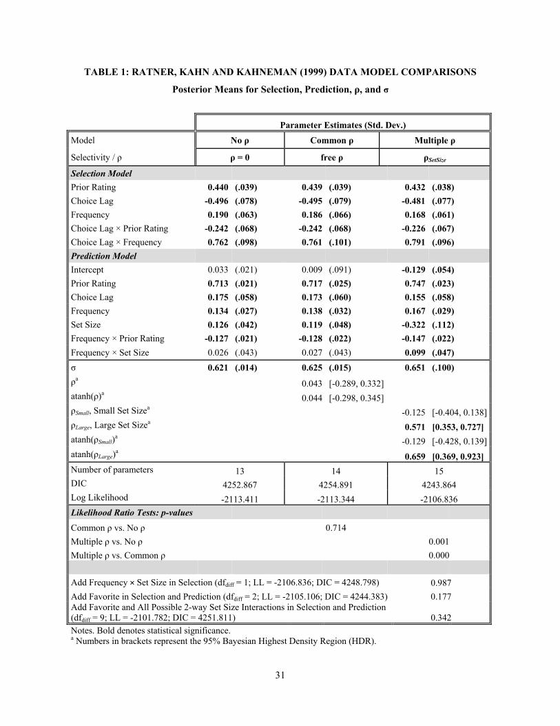
variables, which are mean-centered. Model estimates are given in Table 1.

[Table 1 about here]

We do not engage in a substantive re-interpretation of the very rich RKK data from this

experiment, nor link it to the numerous companion studies in that paper. We can, however, consider

model implications strictly from the vantage point of selectivity, which results do indicate for these data,

as we discuss next. We note here as well that selectivity was similarly indicated for a wide range of

combinations of covariate effects, arguing against its significance being an artifact of the particular

covariate specification for the “best” model.

Results

We discuss three models, in order of their appearance in TABLE 1: (1) assuming no selectivity

(restricting ρ = 0); (2) allowing for an identical degree of selectivity across conditions (free ρ); and (3)

allowing selectivity to vary across choice set conditions (ρSetSize). In this way, one can ‘decompose’ the

influences of the various modeling constructs systematically. Because all parameters are estimated via

Bayesian techniques, we assess significance via Highest Density Regions (HDR) for posteriors. Thus,

‘significant’ denotes zero lies outside a specific HDR, usually at the .05 level, although for convenience

we list traditional means and standard errors.

Item Selectivity. The model estimates reveal an intriguing and, to our knowledge, novel pattern

of selection effects across conditions. Allowing for selection, but assuming ρ equal across (choice set

size) conditions, yields a ρ estimate that is not significantly different from zero ( 0.043, HDR = [-

0.289, 0.332]). This would appear to suggest there are no selection effects for these data. However,

allowing ρ to vary by condition reveals significant selectivity – but only for the larger choice set

                                                            6 Including the same covariates in the Selection and Prediction submodels is permissible, particularly so when, as here, theory suggests doing so. In particular, omitting PRIOR in the selection model might literally give rise to a large value of ρ. Set Size cannot appear in the selection model, as it is constant within choice condition. An additional covariate representing the highest ranked item in each set (Favorite) was also tested in the Selection and Prediction submodels; it was not statistically significant and is not discussed further.

13  

condition: ( -0.125, HDR = [-0.404, 0.138]; 0.571, HDR = [0.353, 0.727]).

Substantively, degree of selectivity increases with choice set size, that is, as the number of foregone

alternatives is also likely to increase. Specifically, we find no significant selection effects for the small

choice set, when the number of choice occasions (ten) far exceeds the number of available items (three);

in the small choice set, respondents have ample opportunity to sample each item at least once, should they

wish to. By contrast, in the larger choice set, respondents are less likely to select every available item, so

the potential for never sampling one or more items (and subsequent selectivity artifacts) increases.

Estimated Effects. Importantly, we also find that allowing for selectivity by condition impacts

estimated effect sizes. Substantively, the pattern of effects for the selection model is of lesser interest, as

coefficients across the various models (in Table 1) are very close; HDRs overlap to a degree that render

them statistically indistinguishable. A very different story emerges across the Prediction models. Given

that, in this application, ρ is only significant in one of the conditions (large set size), we do not expect to

see strong changes in the values of the coefficients that are in both parts of the model. However, these

results still hold directionally: Prior Ratingis slightly more positive, whether a song was chosen last time

(Choice Lag) slightly less positive, and how frequently an item has been chosen (Frequency) slightly

more positive overall in Prediction.

The most striking result is that the effects of Set Size are vastly different across models. When

there is no selection (ρ = 0) or equal selection across choice set size conditions (common ρ), the effects of

Set Size are significantly positive and not statistically distinguishable (β , 0.126, no ρ; β ,

= 0.119, common ρ). That is, if one analyzed only the Rating (i.e., Prediction) data, choice set size could

be confidently claimed as positively affecting evaluation. However, when selectivity is accounted for

across set size conditions ( ), we see that Set Size has a strongly negative effect (β , = -

0.322, p < .003, multiple ρ). This is consistent with extant literature demonstrating that consumers tend to

be less satisfied with items chosen from relatively larger assortments (e.g. Iyengar and Lepper 2000;

Diehl and Poynor 2010). A posteriori, in comparing a choice set of size 3 to one of size 6 (as RKK did),

14  

chosen items are rated about 32% lower, on average, when chosen from the larger set. The valence of an

important main effect is therefore reversed when the Ratings data are analyzed in the absence of an

associated model for choice that not only allows for selectivity, but that also does not restrict selectivity to

be fixed across experimental conditions.

The interaction between Set Size and how frequently an item has been chosen(Frequency) also

has strongly differing effects. When selectivity is not accounted for by condition, the interaction effect is

not significantly different from zero, β , = 0.03 (p > .27, ρ = 0). However, when

selectivity is allowed to vary across conditions (ρSetSize), the interaction between Frequency and Set Size

becomes larger and significant, β , = 0.099 (p < .05). In other words, the more frequently

an item has been chosen, the weaker the effect of set size becomes, suggesting that more consistent choice

sequences are less prone to set size effects on evaluation.

Model Fit. Finally, one is left with the question of which model represents the data best, which

can be assessed via both Bayesian and classical metrics. DIC speaks clearly for multiple ρ, the values of

which, for {no ρ, free ρ, and multiple ρ}, are {4253, 4255, 4244}7. Likelihood ratio tests corroborate the

DIC comparison, while allowing statistical tests for nested models (like those in Table 1): the model

allowing selection to vary by choice set size (multiple ρ) offers a better fit for the data than both the

model with no selection (no ρ; LLdiff = 6.58, df = 2, p < .002) and the model restricting selection to be

equal across set size conditions (common ρ; LLdiff = 6.51, df = 1, p < .001). The models with no selection

versus equal selection across set size conditions exhibit no difference in fit (no ρ vs. common ρ; LLdiff =

0.07, df = 1, p > .7); this is consistent with the non-significance of ρ when it is restricted to be constant

across experimental conditions. The slightly less parsimonious model thus more than compensates for its

additional complexity, and allowing the correlation between selection and prediction to differ across

conditions not only improves fit, but affects interpretation of focal substantive effects.                                                             7 We also performed tests of model fit to demonstrate that no other relevant and potentially significant covariates had been excluded from our focal model. Three tests of significance are summarized at the bottom of Table 1: adding a Frequency × Set Size interaction to the Selection submodel does not improve model fit (p > .98), nor does adding a “Favorite” item indicator variable main effect (p > .17) and all possible 2-way interactions in Selection and Prediction (p > .34).

15  

STUDY 2

The previous analysis, based on data collected in a classic prior experimental study, demonstrated

the potential for selection effect strength to vary across experimental conditions with differing choice set

sizes. Study 2 was designed and conducted with an explicit goal in mind: to examine whether the same

potential exists for another well-known repeated choice phenomenon that has been well documented in

the marketing and psychology literatures. Numerous prior studies have observed that people choosing

multiple items at once now, to consume later, tend to choose a more varied set of items than if they had

chosen the items one-at-a-time, just before consuming each one (e.g., Simonson 1990, Read and

Loewenstein 1995). While prior research has focused on the impact of these two choice modes on

variety-seeking, we will instead focus our analysis on evaluation of the chosen items. More specifically,

we examine the influence of the size of the available choice set on evaluation and selectivity.

Participants chose three snacks, either from a set of six snacks or from a set of twelve snacks.

Half the participants chose all three snacks at once (“simultaneous choice”); the remaining participants

chose each snack one-at-a-time across three choice occasions (“sequential choice”). A 2 (simultaneous

choice vs. sequential choice) X 2 (small choice set vs. large choice set) between-subjects design was

employed.

Snacks included well-known brands of crackers, chips, candy bars, cookies, and nuts. The small

set condition included six snack options, and the large set condition included those six snacks plus six

more. The small set condition stimuli and task replicate experiments found in Simonson (1990) and Read

and Loewenstein (1995). The six additional snacks in the large set were chosen to mirror the six snacks in

the small choice set, in terms of both product attributes and market share, so as not to increase perceptions

of attribute variety or general product desirability. One hundred four undergraduate students participated

in the study to earn course credit in an introductory marketing course.

The study was composed of four sessions spaced one week apart. In session one, participants’

prior preferences were measured; participants rated how much they liked each snack using an 11-point

Likert scale (“1” = dislike very much, “11” = like very much). Participants also ranked the snacks from

16  

their most favorite to their least favorite. The choice tasks took place during sessions two, three and four;

we refer to these as choice weeks one, two, and three, respectively. Participants in the sequential

condition chose and ate one snack in choice week one, chose and ate a second snack during week two,

and chose and ate a third snack in week three. Participants in the simultaneous condition selected all

three snacks in choice week one, designating the first snack to be eaten in choice week one, the second

snack in choice week two, and the third in choice week three. Immediately after participants ate each of

their chosen snacks, they rated how much they liked the snack using an 11-point Likert scale (“1” =

dislike very much, “11” = like very much).

The snack evaluation rating measured immediately after a participant ate his/her chosen snack is

the dependent variable, and it is observed only for the single item chosen for that time period. Regressors

for the selection model (for which item is chosen) are Prior Rating(the a priori item rating),Favorite

(whether the item was designated the favorite; a priori rank equals one), Choice Lag (whether the item

had been chosen in the prior time period), Choice Lag× Favorite interaction, and Choice Lag× SEQ,

where “SEQ” represents the choice mode manipulation (equals one for sequential choice, zero for

simultaneous choice) and. The regressors for the prediction model (for the single brand chosen) include

Prior Rating, Favorite, Choice Lag, and Choice Lag × Favorite interaction, as well as Set Size (equals one

for the large set, zero for the small set). We explored the entire solution space, as in Study 1, to arrive at

this particular set of model covariates.

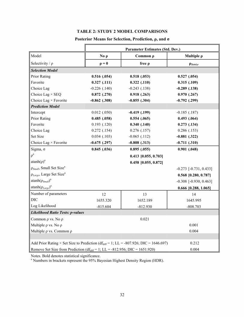
[Table 2 about here]

Results

Item Selectivity. As found in Study 1, results will indicate that ignoring selectivity entails the

possibility of drawing incorrect conclusions. Table 2 summarizes model estimation results in a manner

similar to Study 1, featuring three candidate models that differ in how flexibly they allow for selection: no

selectivity (ρ = 0), selectivity common across conditions (free ρ), and selectivity varying across choice set

conditions (ρSetSize). The pattern of results in Table 2 shows strong evidence of selectivity in the large

17  

choice set condition ( 0.568, HDR = [0.280, 0.787]; multiple ρ), but not in the small choice set

condition ( -0.273, HDR = [-0.731, 0.433]; multiple ρ). This is consistent with the results in

Study 1, and the estimated values of ρSmall and ρLarge are remarkably similar across the two studies. The

model allowing for selectivity, but restricting ρ to be constant across conditions (common ρ), yields an

estimated ρ value that is significantly positive ( 0.413, HDR = [0.055, 0.703]). Thus selection effects

are clearly evident in the data; however, presuming that degree of selectivity is the same across all choice

set conditions would be erroneous in this case, just as in Study 1. Finally, we note that, similar to Study 1,

we observe directional changes in the values of the coefficients that are in both parts of the model: Prior

Rating is more positive, the Choice Lag × Favorite interaction more negative, and Favorite (much) more

positive overall in Prediction.

Estimated Effects. The differences in selectivity reveal their substantive importance when one

compares the estimated Favorite and Set Size effect strengths between the ρ 0 prediction submodel

(i.e., no selection effects at all) and its more flexibly modeled variants. Allowing for common selectivity

yields β , = 0.340 (p < .008; common ρ), a significant effect; presuming there is no selectivity

yields β , = 0.193 (p > .05; ρ = 0), a non-significant value about half the size. Allowing selectivity

to differ across conditions also yields a positive effect of most-favored status, β , = 0.273 (p < .03;

multiple ρ). Thus, allowing for selectivity reveals a crucial role of the favorite option in evaluation: the

most-favored option gets a “boost” in evaluation, over and above that accounted for by its higher prior

rating. Note that a significant negative interaction between Favorite and Choice Lag is observed in all

three models – β , = -0.675 (p < .02) when ρ = 0, β , = -0.808 (p <

.005) when ρ is unrestricted, and β , = -0.711 (p < .02) when ρ is allowed to vary across

set size conditions – suggesting that, in the case where the favorite was chosen in the prior period, the

favorite item’s evaluation is discounted. Thus, for these data, failing to account for selectivity leads to the

erroneous conclusion that the favorite option may be discounted (when chosen repeatedly), but never

18  

“given a boost” in the evaluation process. In other words, a modeling approach that allows for selectivity

reveals the important insight that the favorite option almost always “gets a boost” in evaluation, except in

the case when it was chosen last time.

A second important substantive implication of failing to appropriately account for selectivity is

that the estimated effect of choice set size on evaluation is very different. The pattern of results resembles

that found in Study 1. The estimated effects of Set Size are not distinguishable from zero when there is no

selection (β , = 0.034, p > .37; no ρ) or equal selection across choice set size conditions (β , =

-0.065, p > .28; common ρ). However, when selectivity is accounted for across set size conditions, choice

set size has a very large negative effect (β , = -0.881, p < .004; multiple ρ). This is consistent with

our Study 1 result that, when a model allowing varying degrees of selectivity across choice set conditions

is employed, the results reveal that participants tend to be less satisfied with items chosen from the larger

choice set. This pattern of results is remarkably concordant with study 1, even though that experiment was

run by other researchers, using different stimuli, and with many more repetitions.

Model Fit. Lastly, in addition to the substantive insights gained from allowing for selectivity, we

find better model fits for both models with unrestricted ρ, as measured using DIC: 1655, 1652, and 1646

for no ρ, common ρ, and multiple ρ, respectively. This evidence is bolstered by likelihood ratio tests: the

model with free common ρ offers a better fit than one restricting ρ to zero (LLdiff = 2.67, df = 1, p < .03);

and the model allowing selectivity to vary across choice set conditions fits the data better both than one

restricting ρ to be constant across conditions (LLdiff = 4.23, df = 1, p < .005) and the model restricting ρ to

be zero (LLdiff = 6.90, df = 2, p < .002).8 Overall, analysis of these data provides evidence that

appropriately accounting for selectivity adds substantially to both model fit and interpretation of effects.

STUDY 3

The prior two studies demonstrated that degree of selectivity can vary with the number of

                                                            8 Additional tests of model fit, summarized at the bottom of Table 2, demonstrate that adding Prior Rating × Set Size to the Prediction submodel does not improve model fit (p > .21), and removing Set Size from the Selection submodel significantly reduces model fit (p < .01).

19  

alternatives in a choice set. This study assesses whether selection effects can vary across choice set

conditions even when the number of selection alternatives stays constant. We explore this question with

the same choice task employed in Study 2, and we examine the impact of varying the relative

attractiveness of items in the choice set on degree of selectivity and the value of ρ.

Heckman (1979) noted in his seminal article that if the probability of being included in the

sample is identical for all observations, then estimates of prediction coefficients will not be biased. In the

present choice context, this suggests that when a choice set contains items a decision-maker perceives as

equally attractive, the corresponding prediction model is less prone to selectivity artifacts than if the

choice set contains items with more varied perceived attractiveness levels (which we operationalize here

as a priori rating). We examine the potential relationship between relative attractiveness of choice set

items and degree of selectivity in this study. We define “bunchiness” as the degree to which a choice set

contains items that are perceived to be equally attractive to each other (i.e., the extent to which items are

“bunched” together), from the decision-maker’s perspective. For example, a choice set comprised of six

equally attractive items or one with six equally unattractive items would be high in "bunchiness. Note that

we treat bunchiness as a characteristic of the choice set itself, not as a characteristic of any one item in the

set. We expect that bunchiness will have a negative relationship with degree of selectivity (and ρ).

Participants followed a four week procedure analogous to that in Study 2. They were asked to rate

and rank twelve snacks in week one (the same as those in the Study 2 large set condition). Number of

items chosen together was again manipulated (sequential choice versus simultaneous choice) across three

choice occasions, each separated by one week. Participants evaluated their chosen snacks immediately

after eating each one, using a 1-11 rating scale, as in Study 2. The number of available items was held

constant across conditions, at six, and we manipulated choice set bunchiness. To this end, the items

available in the choice set varied across three bunchiness conditions based on the idiosyncratic rankings

provided by each participant: bunchy-attractive (ranks 1, 2, 3, 4, 5, 12); bunchy-unattractive (ranks 1, 8,

9, 10, 11, 12); and not-bunchy (ranks 1, 4, 6, 8, 10, 12). We include the bunchy-unattractive condition in

the experimental design to assess whether any potential impact of bunchiness is conditional on the

20  

similarly liked alternatives being perceived as (more) attractive; we will allow separate measures of

selectivity for all three conditions, to determine whether, empirically, ρ estimates for bunchy-attractive

and bunchy-unattractive are close in magnitude. Note that all choice sets include both the most-favored

item (rank = 1) and the least-favored item (rank = 12), so that the range of relative attractiveness of all

items in the set is consistent across conditions.

As in Study 2, the snack evaluation rating measured immediately after a participant ate his/her

chosen snack is the dependent variable. Available regressors for the selection and prediction models are

similar to those in Study 2, with the choice set size variable replaced by two binary variables representing

bunchiness: Bunchy Attractive (equals one for the bunchy-attractive condition, zero for not-bunchy and

bunchy-unattractive), and Bunchy Unattractive (equals one for bunchy-unattractive, zero for not-bunchy

and bunchy-attractive). More specifically, the selection submodel regressors are a priori rating (Prior

Rating), a priori most-favored item (Favorite), whether an item was chosen last time (Choice Lag), choice

lag interacted with sequential-simultaneous choice mode (Choice Lag × SEQ), choice lag interacted with

prior rating (Choice Lag × Prior Rating), and most-favored item interacted with the two choice set

condition indicator variables (Bunchy Attractive× Favorite and Bunchy Unattractive× Favorite).

Prediction submodel regressors are Prior Rating, Favorite, Choice Lag, SEQ, Bunchy Attractive, Bunchy

Unattractive, Prior Rating× SEQ, Choice Lag× SEQ, Bunchy Attractive × Prior Rating, Bunchy

Unattractive× Prior Rating, Bunchy Attractive × Favorite, and Bunchy Unattractive× Favorite. As in the

two previous studies, we standardize all variables, except binary (dummy) variables, which are mean-

centered. The model specifications discussed here were the end result of an exhaustive search of the

solution space for each submodel separately, and then that for the conjoined (full) model including

selectivity, similar to the approach used in Studies 1 and 2.

[Table 3 about here]

Results

Item Selectivity. We again find strong evidence of selectivity, this time for all choice set

21  

conditions, with the value of ρ systematically varying with bunchiness. Table 3 presents estimation results

for three models differing in how flexibly selectivity is modeled: no selection (ρ = 0); restricting

selectivity to be constant across choice set conditions (common ρ); and allowing selectivity to differ

across choice set conditions (multiple ρ; ρBunchiness). Restricting ρ to be constant across conditions yields an

estimated ρ value that is significantly positive ( 0.543, HDR = [0.190, 0.788]; common ρ). Allowing ρ

to differ across conditions (ρBunchiness) reveals that degree of selectivity varies with bunchiness: the not-

bunchy choice set produced the greatest degree of selectivity ( 0.835, HDR = [0.578,

0.959]), while the bunchy-attractive and bunchy-unattractive choice sets generated lower, and nearly

identical, degrees of selectivity ( 0.450, HDR = [0.028, 0.740], 0.470,

HDR = [0.040, 0.823]). Consistent with both Studies 1 and 2, we find clear evidence of selection effects

in the data, but it varies in degree across choice set conditions – in this case, without varying choice set

size; decreasing the degree to which available options are perceived as equally attractive (i.e., a “less

bunchy” choice set) increases degree of selectivity.

Estimated Effects. Note that in this application, Rho is significant in all three conditions, and

thus, we expect to see substantial changes in the values of the coefficients that are in both the selection

and prediction submodels. Prior Rating is one standard deviation more positive; Favorite is highly

significant in Selection and doubles in size in Prediction; Prior Rating × SEQ is more negative; Choice

Lag × SEQ nearly doubles in size; and Bunchy Attractive × Favorite grows increasingly negative in

Prediction.

Turning next to the substantive findings, comparing the prediction submodels with increasing

flexibility of accounting for selection, reveals striking differences in four of the prediction covariates:

Favorite, Bunchy Attractive, Bunchy Unattractive, and Choice Lag × SEQ. First, the estimated effect of

Favorite doubles in size when selectivity is accounted for in the model (β , = 0.315, p < .005

when ρ = 0; β , = 0.601, p < .001 with common ρ; β , = 0.640, p < .001 with multiple ρ),

consistent with our finding in Study 2. Second, when selectivity is restricted to be zero (ρ = 0) or common

22  

across choice set conditions (free ρ), Bunchy Attractive and Bunchy Unattractive are estimated to have

negative effects on evaluation (β , = -0.248, p < .02 with common ρ; β , = -0.407,

p < .001 when ρ = 0; β , = -0.390, p < .001 with common ρ). However, when ρ is allowed to

vary across conditions, the estimated effects of Bunchy Attractive and Bunchy Unattractive shrink

dramatically to non-significance (β , = 0.073, p > .36 and β , = -0.093, p > .32

with multiple ρ). This stark change in the estimated effect of choice set condition when ρ is allowed to

vary with bunchiness mirrors the results found in Studies 1 and 2 for the estimated effect of choice set

size condition on evaluation.

Third, we find that the estimated effect of Choice Lag × SEQ without selection (β ,

= 0.279, p > .08; ρ = 0) nearly doubles and becomes statistically significant when selectivity is accounted

for in the model (β , = 0.488, p < .02 with common ρ; β , = 0.536, p < .008

with multiple ρ). Note also that Choice Lag × SEQ always has a positive and significant effect on choice

in the selection submodel (for all estimated models; β , 0.883, p < .001 with multiple ρ),

indicating a tendency toward more inertial choice behavior in the sequential choice mode. Thus, for these

data, failing to account for selectivity would lead the analyst to erroneously conclude that inertial choices

have no distinct effect on evaluation, when they do: an item chosen repeatedly in SEQ receives a “boost”

in evaluation, even after accounting for prior preference rating (Prior Rating).

Model Fit. Finally, we assess model fit and find that it consistently improves as selection is more

flexibly accounted for in the model. Model fit, as measured using DIC, improves when ρ is assumed

constant across choice set conditions (common ρ; 1885 versus 1892), and improves further when ρ is

allowed to vary across choice set conditions (multiple ρ; 1883 versus 1885). Likelihood ratio tests also

indicate that model fit improves: presuming free (common) ρ improves fit versus restricting ρ to zero

(LLdiff = 5.01, df = 1, p < .003); allowing selectivity to vary across choice set conditions improves fit

versus presuming zero ρ (LLdiff = 8.00, df = 2, p < .002); and allowing ρ to vary across choice set

23  

conditions marginally improves model fit versus presuming common ρ (LLdiff = 2.99, df = 1, p ≈ .05).9 In

conclusion, the findings from this study offer further support for the importance of accounting for

selectivity by experimental condition (when warranted), as well as its potential impact on both model fit

and substantive interpretation of effects.

HETEROGENEITY AND FULL ERROR COVARIANCE.

We stress the importance of accounting for “observed” (preference) heterogeneity when

“unobserved” heterogeneity cannot be adequately captured due to the nature of collected data (e.g., few

choices per respondent and/or many potentially heterogeneous regressors; see Andrews et al. 2008). To

emphasize the role of the prior ratings, which serve as “individual differences” in terms of item

preferences in each study, we re-estimate each of the “best” models while omitting Prior Rating in the

Selection submodel, the Prediction submodel, or both. For the RKK data (our Study 1), the “best” model

yields LL of -2106.8 (Table 1; multiple ρ); removing Prior Rating from Selection alters this to -2174.3;

out of Prediction, to -2369.9; out of both to -2683.4; p-values against the “best” model are infinitesimal in

each case (Δ(df) is 1, 1, and 2, respectively, for the LR test, and 2Δ(LL) is over 100 in each case),

although comparatively less so for the Selection submodel. LL for Study 2 was -808.7 for the best model

(Table 2; multiple ρ); removing Prior Rating from Selection yields -878.6; from Prediction, -839.0; from

both, -909.5; p-values are again infinitesimal, although here the smaller difference was for Prediction.

Lastly, for Study 3, LL was -916.0 for the best model (Table 3; multiple ρ); removing Prior Rating from

Selection yields -943.3; from Prediction, -957.7; and from both, -977.3. Yet again, p-values are

infinitesimal, but here the effects for Selection and Prediction are roughly equal. In all three studies,

however, failing to account for observed preference heterogeneity in either submodel produces severe

decrements in model fit. We would again stress that, for researchers estimating such many-parameter

models on limited within-subject choice data, that suitable measures of individual-level preference

                                                            9 Additional tests of model fit confirmed that including Bunchy Attractive × Prior Rating and Bunchy Unattractive × Prior Rating in the Prediction submodel does not improve fit (p > .20), while removing any of the 2-way interactions between the experimental conditions (Bunchy Attractive and Bunchy Unattractive) and Prior Rating or Favorite significantly reduce model fit (all p ≤ .001).

24  

heterogeneity be collected and systematically incorporated in both the Selection and Prediction portions

of the model. We add in closing that we saw no evidence of significant error covariance in any of our data

sets; testing the full covariance probit model against the one used here yielded the following results:

RKK, p = 0.996; Study 2, p = 0.327; Study 3, p = 0.753. We must, of course, stop short of

recommending that empirical researchers fail to account for error covariance in all applications, but the

consistent lack of significance here contrasts sharply with the strong significance in all three studies for ρ,

the central metric for the presence of selectivity.

ITEM SELECTIVITY VERSUS OMITTED VARIABLES

It is well-known that omitted regressors can mimic the effects of authentic selectivity, that is, lead

to significance of the error correlation, ρ. In their recent overview of the literature on making causal

claims, Antonakis et al. (2010) suggest that random field experiments are a “gold standard”, but also

underscore that omitted regressor bias can muddy interpretation in the standard (Heckman) selectivity

framework. For researchers interested in substantive claims about item selectivity, it is therefore critical to

be circumspect regarding the potential for omitted regressors.

General tests for omitted regressors, conceptualized as a specification error, date back to Ramsey

(1969), who introduced the RESET procedure for linear models. Here, we follow Peters (2000), who

demonstrates that a RESET-based procedure applies to a wide range of parametric and semiparametric

model types, as well as how to perform associated Likelihood Ratio and Wald tests, the former being

preferred on statistical grounds. The procedure is straightforward: for any particular model, calculate its

predictions for the observed variables (e.g., ratings, in our context), ; then, re-estimate the model

successively (cumulatively) including new regressors, , for 2, 3, …; note that 1 corresponds to

the regressors already included in the (Prediction) model.

Table 4 lists the results of this procedure for our three data sets, for k = 1, ..., 5 (k > 5 revealed no

new phenomena). For each data set, all five values of k are run for the “multiple ρ” model (i.e., the best-

fitting models, as listed in Tables 1, 2, and 3) and for an analogous model with ρ restricted to zero, that is,

an ordinary regression; classical LL values are listed for all thirty models (3 data sets × 5 values of k × 2

25  

conditions for ρ). Three types of p-values can therefore be calculated: each model vs. k = 1; each model

vs. k being one smaller (“k – 1”); and each “multiple ρ” model vs. ρ = 0 (see footnotes to Table 4 for

fuller descriptions). These appear in successive columns, and tell an especially clear ‘story’. First, there is

mild evidence of model misspecification (i.e., .01 < p < .05) only for the RKK data, and then only for k =

2 (i.e., by including as a regressor); this does not hold for any k vs. k - 1 for k > 2. There is no evidence

whatsoever of misspecification for Studies 2 and 3, with all 32 possible tests having p > .23.

While one might wonder about the RKK data in this regard, the lack of strong evidence for

misspecification is shorn up greatly (and more so in Studies 2 and 3) by the last column of tests, against ρ

= 0. In all cases, these are each in the range of p ≈ .001. That is, tests for including ρ come out at least 10

times stronger (100 times for Studies 2 and 3) than those for including various combinations of . As

such, this largely rules out the omission of as a source for claims of item selectivity, decisively for

Studies 2 and 3 and arguably for RKK. We would strongly caution researchers who wish to test for item

selectivity to run similar RESET-like tests on their resulting models in order to distinguish the strength of

evidence for selectivity from that of possible omitted regressors.

CONCLUSIONS AND POTENTIAL EXTENSIONS

Model frameworks developed by Heckman, Tobin, and others have allowed researchers to

understand the effects of failing to account for selectivity. These models have been applied widely to field

data, since researchers clearly need to comprehend and correct for selectivity effects that they cannot hope

to control. Although the so-called “Heckman model” and related variants have become standard tools for

field data studies in marketing, the need for selectivity correction for laboratory work – which typically

offers the luxury of random assignment to conditions – has been tacitly seen as less pressing, or perhaps

non-existent. It is also possible that the form of the classic Heckman model – a binary selection

mechanism, specifically – may have limited its applicability in behavioral research, where choices are

typically freely made from a set of options, with information collected subsequently.

Our intent in this paper has been to demonstrate that similar selectivity mechanisms are intrinsic

to a broad class of decision problems common in consumer and psychological research, and to show how

26  

researchers can account for them in a general setting. Three studies – one a reanalysis of an influential,

classic data set, and two theory-driven experiments designed specifically for this purpose – converged on

similar conclusions, namely that: selectivity effects can be significant even in fully controlled randomized

laboratory studies; accounting for selectivity can alter some focal substantive results; allowing for

different degrees of selectivity across experimental conditions can be crucial; selectivity appears to follow

predictable patterns in terms of the nature of ‘foregone options’ and ‘similarity of attractiveness’ of

available choice alternatives.

Although we have not reported on them in this paper, we have successfully extended the model to

allow for different types of selection and prediction types, including ‘pick-any’ and ranked selection (i.e.,

the field is narrowed not to just one, but to several, options, which may be ranked) and both ordinal (i.e.,

on a discrete, ordered scale) and discrete choice prediction (i.e., we observe only what was finally chosen,

but not any rating or evaluation of it). A common example of such extensions is the process of purchasing

a car, which typically involves several distinct phases – information-gathering, visiting dealers, test

driving – before a choice is made. Researchers ignoring the individual-specific selection phase(s)

preceding eventual choice may be led astray in gauging just what drives the market. For example, price

may determine which cars are eliminated early on, and may thus appear relatively unimportant if only

later stages of the purchase process are analyzed. Applying an appropriate member of this class of models

would allow one to disentangle the effects of (perhaps multiple phases of) selection, as in Wachtel and

Otter’s (2013) general setting.

We can envision several fruitful extensions of the basic methodology. For example, ‘selection’ in

our model requires full knowledge of available options and item covariates, which are rarely available in

field data, and require care and foresight in experimental settings. Although we have underscored the

importance of observed heterogeneity, a challenge in all discrete choice modeling remains the

incorporation of (unobserved) parametric heterogeneity when there are few observations per respondent,

especially when there is a comparatively large number of estimated coefficients. We have also not

explored, other than by exhaustive search, stepwise, and LARS methods on each of the selection and

27  

prediction submodels separately, how one chooses the best regressor set for the “full” conjoined model;

and, if so, whether forms of stepwise or LARS procedures might be fruitful, given that the covariate space

for the conjoined model can be vast, especially when, as in our applications, interaction effects are

considered. We view these as primarily issues of implementation and processing speed, and to only be

presently prohibitive for models with many regressors or interactions. The models presented here can be

readily estimated using a variety of available software platforms with modest run-times, and as such

would be methods behavioral researchers could readily avail of “out of the box” to determine whether

selectivity effects were presented in their experimental data.

28  

REFERENCES

Albuquerque, P., P. Pavlidis, U. Chatow, K. Y. Chen, and Z. Jamal (2012), Evaluating Promotional Activities in an

Online Two-sided Market of User-generated Content, Marketing Science, 31(3), 406-432.

Anderson, E. T., and D. I. Simester (2004), Long-run Effects of Promotion Depth on New versus Established

Customers: Three Field Studies, Marketing Science, 23(1), 4-20.

Andrews, R. L., A. Ainslie, and I. S. Currim (2008), “On the Recoverability of Choice Behaviors with Random

Coefficients Choice Models in the Context of Limited Data and Unobserved Effects,” Management

Science, 54(1), 83-99.

Antonakis, J., Bendahan, S., Jacquart, P., & Lalive, R. (2010), On Making Causal Claims: A Review and

Recommendations, The Leadership Quarterly, 21(6), 1086-1120.

Berk, R. A. (1983), An Introduction to Sample Selection Bias in Sociological Data, American Sociological Review,

386-398.

Braun, K. A. (1999), Postexperience Advertising Effects on Consumer Memory, Journal of Consumer Research, 25

(March): 219-344.

Broniarczyk, S. M. (2008), Product Assortment, Handbook of Consumer Psychology, eds. C. P. Haugtvedt, P. M.

Herr, and F. R. Kardes, Laurence Erlbaum Associates, 755-779.

Chakravarti, A. and C. Janiszewski (2003), The Influence of Macro-Level Motives on Consideration Set

Composition in Novel Purchase Situations, Journal of Consumer Research, 30(September), 244-258.

Danaher, P. J. (2002), Optimal Pricing of New Subscription Services: Analysis of a Market Experiment, Marketing

Science, 21(2), 119-138.

Degeratu, A. M., A. Rangaswamy and J. Wu (2000), Consumer Choice Behavior in Online and Traditional

Supermarkets: The Effects of Brand Name, Price, and Other Search Attributes, International Journal of

Research in Marketing, 17(1), 55-78.

Diehl, K. and C. Poynor, (2010) Great Expectations?! Assortment Size, Expectations and Satisfaction, Journal of

Marketing Research, 47(April), 312-322

Efron, B., Hastie, T., Johnstone, I., & Tibshirani, R. (2004), Least Angle Regression, The Annals of Statistics, 32(2),

407-499.

Fitzsimons, G. (2000), Consumer Response to Stockouts, Journal of Consumer Research, 27 (September), 249-266.

Hartmann, W. (2006), Comment on Structural Modeling in Marketing, Marketing Science 25(6), pp. 620–621.

Haübl, G. and V. Trifts (2000), Consumer Decision Making in Online Shopping Environments: The Effects of

Interactive Decision Aids, Marketing Science, 19(1), 4-21.

Heckman, J. J. (1976), Common Structure of Statistical-Models of Truncation, Sample Selection And Limited

Dependent Variables And a Simple Estimator For Such Models, Annals of Economic And Social Measurement,

5(4), 475-492.

29  

Heckman, J. J. (1979), Sample Selection Bias as a Specification Error, Econometrica, 47(1), 153-161.

Heckman, J. (1990), Varieties of Selection Bias, The American Economic Review, 80(2), 313-318.

Heckman, J., H. Ichimura, J. Smith, and P. Todd, (1998). Characterizing Selection Bias Using Experimental

Data (No. w6699), National Bureau of Economic Research.

Iyengar, S. and M. Lepper (2000), When Choice is Demotivating: Can One Desire Too Much of a Good Thing?,

Journal of Personality and Social Psychology, 79(6), 995-1006.

Jedidi, K., C. F. Mela, and S. Gupta (1999), Managing Advertising and Promotion for Long-run

Profitability, Marketing Science, 18(1), 1-22.

Kahneman, D., P.P. Wakker, and R. Sarin (1997), Back to Bentham? Explorations of Experienced Utility, Quarterly

Journal of Economics, 112, May, 375-405.

Krishnamurthi, L., and S. P. Raj (1988), A Model of Brand Choice and Purchase Quantity Price

Sensitivities, Marketing Science, 7(1), 1-20.

Lambrecht, A., K. Seim, and C. Tucker (2011), Stuck in the Adoption Funnel: The Effect of Interruptions in the

Adoption Process on Usage, Marketing Science, 30(2), 355-367.

Lee, L. F. (1983), Generalized Econometric Models With Selectivity, Econometrica, 51, 507-512.

Levin, I. P., J. D. Jasp and W. S. Forbes (1998), Choosing Versus Rejecting Options at Different Stages of Decision

Making, Journal of Behavioral Decision Making, 11: 193-210.

Levin, I. P., C. M. Prosansky, D. Heller, and B. M. Brunicck (1991), Prescreening of Choice Options in ‘Positive’

and ‘Negative’ Decision-Making Tasks, Journal of Behavioral Decision Making, 14: 279-293.

Litt, A., & Tormala, Z. L. (2010), Fragile Enhancement of Attitudes and Intentions Following Difficult Decisions,

Journal of Consumer Research, 37(4), 584-598.

McCulloch, R., N. Polson and P. Rossi (2000), Bayesian Analysis of the Multinomial Probit Model with Fully

Identified Parameters, Journal of Econometrics, 99, 173-193.

Moe, W. W., and D. A. Schweidel (2012), Online Product Opinions: Incidence, Evaluation, and

Evolution, Marketing Science, 31(3), 372-386.

Nelson, F. D. (1984), Efficiency of the 2-Step Estimator For Models With Endogenous Sample Selection, Journal of

Econometrics, 24 (1-2), 181-196.

Peters, S. (2000), On the Use of the RESET Test in Microeconometric Models, Applied Economics Letters, 7(6),

361-365.

Puhani, P. A. (2000), The Heckman Correction for Sample Selection and its Critique, Journal of Economic Surveys,

14(1), 53-68.

Ramsey, J. B. (1969), Tests for Specification Errors in Classical Linear Least-Squares Regression Analysis, Journal

of the Royal Statistical Society: Series B (Statistical Methodological), 350-371.

Ratner, R. K., B. E. Kahn and D. Kahneman (1999), Choosing Less-Preferred Experiences for the Sake of Variety,

30  

Journal of Consumer Research, 26(1), 1-15.

Read, D. and G. Loewenstein (1995), Diversification Bias: Explaining the Discrepancy in Variety Seeking Between

Combined and Separated Choices, Journal of Experimental Psychology: Applied, 1 (1), 34-49.

Reinartz, W., J. S. Thomas, and V. Kumar (2005), Balancing Acquisition and Retention Resources to Maximize

Customer Profitability, Journal of Marketing, 69(1), 63-79.

Rost, J. (1985), A Latent Class Model for Rating Data, Psychometrika, 50, 37-49.

Shiv, B. and J. Huber (2000), The Impact of Anticipating Satisfaction on Consumer Choice, Journal of Consumer

Research, 27 (September): 202-216.

Simonson, I. (1990), The Effect of Purchase Quantity and Timing on Variety-Seeking Behavior, Journal of

Marketing Research, 27 (May), 150-162.

Spiegelhalter, D.J., N.G. Best, B.P. Carlin, and A. van der Linde (2002), Bayesian Measures of Model Complexity

and Fit, Journal of the Royal Statistical Society, Series B, 64, 583-639.

Tobin, J. (1958), Estimation of Relationships Among Limited Dependent Variables, Econometrica, 26, 24--36.

Tversky, A. (1972), Elimination by Aspects: A Theory of Choice, Psychological Review, 79, 281-299.

Vella, F. (1998), Estimating Models with Sample Selection Bias: A Survey, Journal of Human Resources, 127-169.

Van Nierop, E., Bronnenberg, B., Paap, R., Wedel, M., & Franses, P. H. (2010). Retrieving unobserved

consideration sets from household panel data. Journal of Marketing Research, 47(1), 63-74.

Wachtel, S., & T. Otter (2013). Successive Sample Selection and Its Relevance for Management

Decisions. Marketing Science, 32(1), 170-185.

Wedel, M., W. A. Kamakura, A. C. Bemmaor, J. Chiang, T. Elrod, R. Johnson, P. J. Lenk, S. A. Neslin, and C. S.

Poulsen (1999), Discrete and Continuous Representation of Heterogeneity, Marketing Letters, 10 (3), 217-30.

Winship, C. and R. D. Mare (1992), Models For Sample Selection Bias, Annual Review of Sociology, 18, 327-350.

Yang, S., M. M. Hu, R. S. Winer, H. Assael, and X. Chen (2012), An Empirical Study of Word-of-Mouth

Generation and Consumption, Marketing Science, 31(6), 952-963.

Ying, Y., F. Feinberg, and M. Wedel (2006), Leveraging Missing Ratings to Improve Online Recommendation

Systems, Journal of Marketing Research, 43(3), 355-365.

Zhang, S. and G. Fitzsimons (1999), Choice Process Satisfaction: The Influence of Attribute Alignability and Option

Limitation, Organizational Behavior and Human Decision Processes, 77 (3), 192-214.

31  

TABLE 1: RATNER, KAHN AND KAHNEMAN (1999) DATA MODEL COMPARISONS

Posterior Means for Selection, Prediction, ρ, and σ

 

Parameter Estimates (Std. Dev.)

Model No ρ Common ρ Multiple ρ

Selectivity / ρ ρ = 0 free ρ ρSetSize

Selection Model

Prior Rating 0.440 (.039) 0.439 (.039) 0.432 (.038)

Choice Lag -0.496 (.078) -0.495 (.079) -0.481 (.077)

Frequency 0.190 (.063) 0.186 (.066) 0.168 (.061)

Choice Lag × Prior Rating -0.242 (.068) -0.242 (.068) -0.226 (.067)

Choice Lag × Frequency 0.762 (.098) 0.761 (.101) 0.791 (.096)

Prediction Model Intercept 0.033 (.021) 0.009 (.091) -0.129 (.054)

Prior Rating 0.713 (.021) 0.717 (.025) 0.747 (.023)

Choice Lag 0.175 (.058) 0.173 (.060) 0.155 (.058)

Frequency 0.134 (.027) 0.138 (.032) 0.167 (.029)

Set Size 0.126 (.042) 0.119 (.048) -0.322 (.112)

Frequency × Prior Rating -0.127 (.021) -0.128 (.022) -0.147 (.022)

Frequency × Set Size 0.026 (.043) 0.027 (.043) 0.099 (.047)

σ 0.621 (.014) 0.625 (.015) 0.651 (.100)

ρa 0.043 [-0.289, 0.332] atanh(ρ)a 0.044 [-0.298, 0.345] ρSmall, Small Set Sizea -0.125 [-0.404, 0.138]ρLarge, Large Set Sizea 0.571 [0.353, 0.727] atanh(ρSmall)

a -0.129 [-0.428, 0.139]

atanh(ρLarge)a 0.659 [0.369, 0.923]

Number of parameters 13 14 15 DIC 4252.867 4254.891 4243.864 Log Likelihood -2113.411 -2113.344 -2106.836

Likelihood Ratio Tests: p-values

Common ρ vs. No ρ 0.714

Multiple ρ vs. No ρ 0.001

Multiple ρ vs. Common ρ 0.000

Add Frequency × Set Size in Selection (dfdiff = 1; LL = -2106.836; DIC = 4248.798) 0.987

Add Favorite in Selection and Prediction (dfdiff = 2; LL = -2105.106; DIC = 4244.383) 0.177 Add Favorite and All Possible 2-way Set Size Interactions in Selection and Prediction (dfdiff = 9; LL = -2101.782; DIC = 4251.811) 0.342

Notes. Bold denotes statistical significance. a Numbers in brackets represent the 95% Bayesian Highest Density Region (HDR).

 

32  

TABLE 2: STUDY 2 MODEL COMPARISONS

Posterior Means for Selection, Prediction, ρ, and σ

Parameter Estimates (Std. Dev.)

Model No ρ Common ρ Multiple ρ

Selectivity / ρ ρ = 0 free ρ ρSetsize

Selection Model

Prior Rating 0.516 (.054) 0.518 (.053) 0.527 (.054)

Favorite 0.327 (.111) 0.322 (.110) 0.315 (.109)

Choice Lag -0.226 (.140) -0.243 (.138) -0.289 (.138)

Choice Lag × SEQ 0.872 (.270) 0.918 (.263) 0.970 (.267)

Choice Lag × Favorite -0.862 (.308) -0.855 (.304) -0.792 (.299)

Prediction Model Intercept 0.012 (.050) -0.419 (.199) -0.185 (.187)

Prior Rating 0.485 (.058) 0.554 (.065) 0.493 (.064)

Favorite 0.193 (.120) 0.340 (.140) 0.273 (.134)

Choice Lag 0.272 (.154) 0.276 (.157) 0.286 (.153)

Set Size 0.034 (.103) -0.065 (.112) -0.881 (.322)

Choice Lag × Favorite -0.675 (.297) -0.808 (.313) -0.711 (.310)

Sigma, σ 0.845 (.036) 0.895 (.055) 0.901 (.048)

ρa 0.413 [0.055, 0.703] atanh(ρ)a 0.458 [0.055, 0.872] ρSmall, Small Set Sizea -0.273 [-0.731, 0.433] ρLarge, Large Set Sizea 0.568 [0.280, 0.787] atanh(ρSmall)

a -0.308 [-0.930, 0.463]

atanh(ρLarge)a 0.666 [0.288, 1.065]

Number of parameters 12 13 14 DIC 1655.320 1652.189 1645.995 Log Likelihood -815.604 -812.930 -808.703

Likelihood Ratio Tests: p-values

Common ρ vs. No ρ 0.021

Multiple ρ vs. No ρ 0.001

Multiple ρ vs. Common ρ 0.004

Add Prior Rating × Set Size to Prediction (dfdiff = 1; LL = -807.926; DIC = 1646.697) 0.212

Remove Set Size from Prediction (dfdiff = 1; LL = -812.956; DIC = 1651.920) 0.004

Notes. Bold denotes statistical significance. a Numbers in brackets represent the 95% Bayesian Highest Density Region (HDR).

 

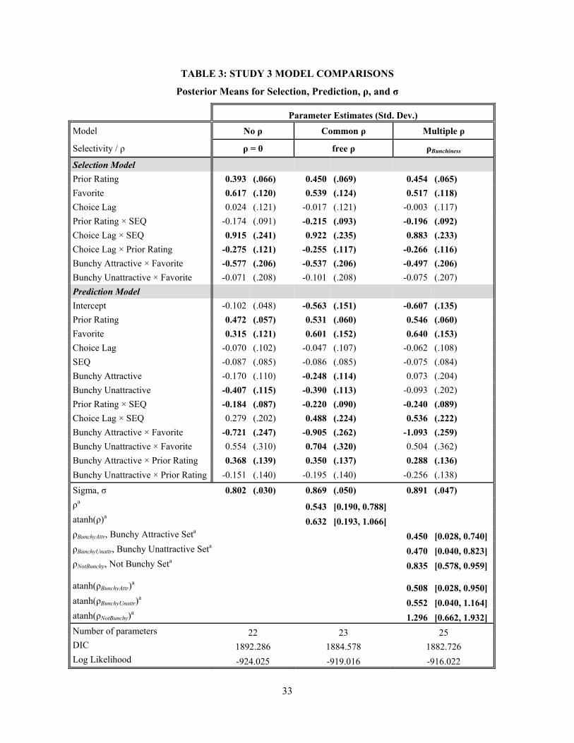
33  

TABLE 3: STUDY 3 MODEL COMPARISONS

Posterior Means for Selection, Prediction, ρ, and σ

Parameter Estimates (Std. Dev.)

Model No ρ Common ρ Multiple ρ

Selectivity / ρ ρ = 0 free ρ ρBunchiness

Selection Model

Prior Rating 0.393 (.066) 0.450 (.069) 0.454 (.065)

Favorite 0.617 (.120) 0.539 (.124) 0.517 (.118)

Choice Lag 0.024 (.121) -0.017 (.121) -0.003 (.117)

Prior Rating × SEQ -0.174 (.091) -0.215 (.093) -0.196 (.092)

Choice Lag × SEQ 0.915 (.241) 0.922 (.235) 0.883 (.233)

Choice Lag × Prior Rating -0.275 (.121) -0.255 (.117) -0.266 (.116)

Bunchy Attractive × Favorite -0.577 (.206) -0.537 (.206) -0.497 (.206)

Bunchy Unattractive × Favorite  -0.071 (.208) -0.101 (.208) -0.075 (.207)

Prediction Model             Intercept -0.102 (.048) -0.563 (.151) -0.607 (.135)

Prior Rating 0.472 (.057) 0.531 (.060) 0.546 (.060)

Favorite 0.315 (.121) 0.601 (.152) 0.640 (.153)

Choice Lag -0.070 (.102) -0.047 (.107) -0.062 (.108)

SEQ -0.087 (.085) -0.086 (.085) -0.075 (.084)

Bunchy Attractive -0.170 (.110) -0.248 (.114) 0.073 (.204)

Bunchy Unattractive -0.407 (.115) -0.390 (.113) -0.093 (.202)

Prior Rating × SEQ -0.184 (.087) -0.220 (.090) -0.240 (.089)

Choice Lag × SEQ 0.279 (.202) 0.488 (.224) 0.536 (.222)

Bunchy Attractive × Favorite -0.721 (.247) -0.905 (.262) -1.093 (.259)

Bunchy Unattractive × Favorite 0.554 (.310) 0.704 (.320) 0.504 (.362)

Bunchy Attractive × Prior Rating 0.368 (.139) 0.350 (.137) 0.288 (.136)

Bunchy Unattractive × Prior Rating -0.151 (.140) -0.195 (.140) -0.256 (.138)

Sigma, σ 0.802 (.030) 0.869 (.050) 0.891 (.047)

ρa 0.543 [0.190, 0.788] atanh(ρ)a 0.632 [0.193, 1.066] ρBunchyAttr, Bunchy Attractive Seta 0.450 [0.028, 0.740] ρBunchyUnattr, Bunchy Unattractive Seta 0.470 [0.040, 0.823] ρNotBunchy, Not Bunchy Seta 0.835 [0.578, 0.959]

atanh(ρBunchyAttr)a 0.508 [0.028, 0.950]

atanh(ρBunchyUnattr)a 0.552 [0.040, 1.164]

atanh(ρNotBunchy)a 1.296 [0.662, 1.932]

Number of parameters 22 23 25 DIC 1892.286 1884.578 1882.726 Log Likelihood -924.025 -919.016 -916.022

34  

TABLE 3 (Continued): STUDY 3 MODEL COMPARISONS

Posterior Means for Selection, Prediction, ρ, and σ

Parameter Estimates (Std. Dev.)

Model No ρ Common ρ Multiple ρ

Selectivity / ρ ρ = 0 free ρ ρBunchiness

Likelihood Ratio Tests: p-values

Common ρ vs. No ρ 0.002

Multiple ρ vs. No ρ 0.001

Multiple ρ vs. Common ρ 0.050

Add Bunchy Attractive × Prior Rating and Bunchy Unattractive × Prior Rating to Selection

(dfdiff = 2; LL = -914.455; DIC = 1884.891) 0.209

Remove Bunchy Attractive × Prior Rating and Bunchy Unattractive × Prior Rating from Prediction

(dfdiff = 2; LL = -922.901; DIC = 1893.562) 0.001

Remove Bunchy Attractive × Favorite and Bunchy Unattractive × Favorite from Selection and Prediction

(dfdiff = 4; LL = -926.867; DIC = 1930.359) 0.000

Remove All Six Interactions With Bunchy Attractive or Bunchy Unattractive

(dfdiff = 6; LL = -932.080; DIC = 1903.188) 0.000

Remove Bunchy Attractive and Bunchy Unattractive and All Six Interactions With Them

(dfdiff = 8; LL = -932.739; DIC = 1899.766) 0.000

Notes. Bold denotes statistical significance. a Numbers in brackets represent the 95% Bayesian Highest Density Region.

 

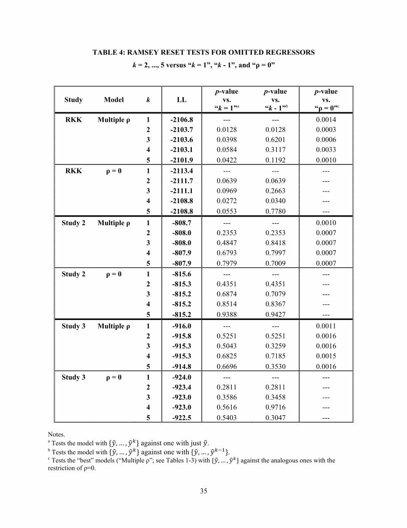
35  

TABLE 4: RAMSEY RESET TESTS FOR OMITTED REGRESSORS

k = 2, ..., 5 versus “k = 1”, “k - 1”, and “ρ = 0”

Study

Model

k

LL

p-value vs.

“k = 1”a

p-value vs.

“k - 1”b

p-value vs.

“ρ = 0”c

RKK Multiple ρ 1 -2106.8 --- --- 0.0014 2 -2103.7 0.0128 0.0128 0.0003 3 -2103.6 0.0398 0.6201 0.0006 4 -2103.1 0.0584 0.3117 0.0033

5 -2101.9 0.0422 0.1192 0.0010

RKK ρ = 0 1 -2113.4 --- --- --- 2 -2111.7 0.0639 0.0639 --- 3 -2111.1 0.0969 0.2663 --- 4 -2108.8 0.0272 0.0340 ---

5 -2108.8 0.0553 0.7780 ---

Study 2 Multiple ρ 1 -808.7 --- --- 0.0010 2 -808.0 0.2353 0.2353 0.0007 3 -808.0 0.4847 0.8418 0.0007 4 -807.9 0.6793 0.7997 0.0007

5 -807.9 0.7979 0.7009 0.0007

Study 2 ρ = 0 1 -815.6 --- --- --- 2 -815.3 0.4351 0.4351 --- 3 -815.2 0.6874 0.7079 --- 4 -815.2 0.8514 0.8367 ---

5 -815.2 0.9388 0.9427 ---

Study 3 Multiple ρ 1 -916.0 --- --- 0.0011 2 -915.8 0.5251 0.5251 0.0016 3 -915.3 0.5043 0.3259 0.0016 4 -915.3 0.6825 0.7185 0.0015

5 -914.8 0.6696 0.3530 0.0016

Study 3 ρ = 0 1 -924.0 --- --- --- 2 -923.4 0.2811 0.2811 --- 3 -923.0 0.3586 0.3458 --- 4 -923.0 0.5616 0.9716 ---

5 -922.5 0.5403 0.3047 --- Notes. a Tests the model with , … , against one with just . b Tests the model with , … , against one with , … , . c Tests the “best” models (“Multiple ρ”; see Tables 1-3) with , … , against the analogous ones with the restriction of ρ=0.