WHEN IT RAINS, IT POURS: UNDER WHAT CIRCUMSTANCES DOES JOB LOSS LEAD TO DIVORCE

By

Melissa Ruby Banzhaf U.S. Census Bureau

CES 13-62 December, 2013

The research program of the Center for Economic Studies (CES) produces a wide range of economic analyses to improve the statistical programs of the U.S. Census Bureau. Many of these analyses take the form of CES research papers. The papers have not undergone the review accorded Census Bureau publications and no endorsement should be inferred. Any opinions and conclusions expressed herein are those of the author(s) and do not necessarily represent the views of the U.S. Census Bureau. All results have been reviewed to ensure that no confidential information is disclosed. Republication in whole or part must be cleared with the authors.

To obtain information about the series, see www.census.gov/ces or contact Fariha Kamal, Editor, Discussion Papers, U.S. Census Bureau, Center for Economic Studies 2K132B, 4600 Silver Hill Road, Washington, DC 20233, CES.Papers.List@census.gov.

Abstract

Much of the previous research that has examined the effect of job loss on the probability of divorce rely on data from the 1970s-80s, a period of dramatic change in marital formation and dissolution. It is unclear how well this research pertains to more recent trends in marriage, divorce, and female labor force participation. This study uses data from the Survey of Income and Program Participation (SIPP) from 2000 to 2012 (thus including effects of the Great Recession) to examine how displacement (i.e., exogenous job loss) affects the probability of divorce. The author finds clear evidence that the effects of displacement appear to be asymmetric depending upon the gender of the job loser. Specifically, displacement significantly increases the probability of divorce but only if the husband is the spouse that is displaced and his earnings represented approximately half of the household’s earnings prior to displacement. Similarly, results show that the probability of divorce increases if the wife is employed and as her earnings increase. While the mechanism behind these asymmetric results remains unclear, these results are consistent with recent research that finds a destabilizing effect on marriages when a wife earns more than her husband.

Keywords: divorce, job loss, displacement JEL codes: J12, J63

* Melissa Ruby Banzhaf, Administrator, Atlanta Census Research Data Center at the Federal Reserve Bank of Atlanta, 1000 Peachtree St. NE, Atlanta, GA 30309. Email: mbanzhaf@frbatlanta.org. Disclaimer: Any opinions and conclusions expressed herein are those of the author and do not necessarily represent the views of the U.S. Census Bureau. All results have been reviewed to ensure that no confidential information is disclosed. The author would like to thank Animesh Giri for providing research assistance, and Kristin McCue and Laura Argys for helpful comments. The author also thanks participants at the 2012 Southern Economic Association annual meeting and seminar participants at Georgia State University and the U.S. Census Bureau for providing valuable feedback.

Section 1: Introduction

As a result of the “Great Recession” in December 2007, 8.8 million jobs were lost. Even though

the recession officially ended in June 2009, unemployment rates have been slow to improve. Although

the macro consequences of job loss have received much attention, there are also important micro

consequences to be considered. One of these is the effect of job loss on marital stability.

After peaking in 1981, the average divorce rate in the U.S. population has been steadily

declining. As Stephenson and Wolfers (2007) document, part of this fall is attributable to lower

marriage rates in the population. However, even after controlling for declines in marriage, the divorce

rate for married couples “at risk” of divorce has fallen more than twenty percent since its peak. In

addition to changes in divorce, recently studies have documented changes in marital matching since the

1970s. For example, Bredemeier and Juessen (2013) find that there has been an increase in assortative

mating leading to changes in the patterns of female labor force participation.

Hellerstein and Morrill (2011) have recently examined the effect of macroeconomic shocks on

aggregate divorce rates and find that, at the state level, an increase in the unemployment rate is

associated with a decline in divorce rates. However, less is known about the effect of job loss on the

probability of divorce at the household level. Studies such as Charles and Stephens (2004) and Weiss

and Willis (1997) that do examine the effect of job loss or negative income shocks on the probability of

divorce rely on data from the 1970s-80s, a period of dramatic change in marital formation and

dissolution. Although Doiron and Mendolia (2011) analyze job loss on family dissolution within the past

decade, they use British household data and include cohabitations in their analysis. It is unclear how

well their findings extend to the institutional frameworks underlying marriage and divorce, not to

mention job loss, in the United States.

Why should economists care if job loss negatively affects marriage? Studies have shown divorce

to have mostly negative economic and social consequences, even after controlling for selection issues.

1

Many of these studies have documented negative effects of divorce on children with respect to

educational outcomes (Painter and Levine 2000; Tartari 2007, Gruber 2004), earnings (Corak 2001; Kane

et al. 2010), and emotional development (Gruber 2004, Amato 2000, Biblarz and Gottainer 2004). In

addition, studies such as Page and Stephens (2004) have also shown negative short-term and long-term

effects on family income resulting from divorce. Because job loss was so pervasive in the Great

Recession and because divorce can have long-term consequences both for children and adults, it is

important to better understand how job loss affects the probability of divorce in order to identify factors

that might weaken this link.

In contrast to Charles and Stephens (2004) and Doiron and Mendolia (2011) who included

terminations, layoffs, and displacements in their analyses of job loss, this study limits job loss to

involuntary displacement resulting from reduced business demand or firm closing. I assume that this

displacement is exogenous to the individual and not a result of the individual’s personal characteristics

or job performance. Terminations that result from firings are not included in this analysis since

unobserved factors of the individual may affect both the probability of being fired and the probability of

divorce (such as violent temperament, laziness, etc.), leading to biased results.

The objective of this study is to identify the circumstances under which displacement may

increase the probability of divorce. Unlike Doiron and Mendolia (2011), this study examines the

displacement of both husbands and wives, and determines if the sex of the job loser impacts the

probability of divorce. That is, is divorce more likely to follow if the man or the woman loses a job?

One important aspect of the most recent recession is that men experienced unemployment at much

higher rates than women. The unemployment rate for men peaked at 10.7 percent compared with 8.3

percent for women. In contrast, the peak unemployment rates for men and women were much closer

in the 2001 recession, 6.0 percent for men compared with 5.3 percent for women. Do these

discrepancies in unemployment rates translate into differential rates of divorce, all other things equal?

2

Second, this study analyzes how the percentage of family earnings lost from displacement

affects the probability of divorce. The predictions of economic theory, discussed in section 3, are

ambiguous; losing a larger proportion of family earnings could generate greater marital stress,

increasing the likelihood of divorce. However, the loss of a larger percentage of family earnings also

may reduce the ability of a couple to finance divorce. Taken at the limit, if the sole earner loses his or

her job, it may be that neither spouse can afford to divorce due to liquidity constraints. In this study, I

test for both linear and nonlinear effects of the percentage of lost earnings on the probability of divorce.

Third, this study examines how the duration of the unemployment spell affects the probability

of divorce. The peak average unemployment spell at 40 weeks in the Great Recession was double the

length of the peak average unemployment spell in the 2001 recession. One would expect that all else

equal, longer unemployment spells would increase the probability of marital dissolution.

Finally, this study assesses whether the employment characteristics of the non-displaced spouse

affect the probability of divorce. Using Census Bureau data, the proportion of dual-earner households

has grown from 29 percent in 1970 to about 54 percent in 2007, the year before the Great Recession

began. This trend reinforces the need for current research on the relationship between job

displacement and divorce since marriages may react differently to displacement than in prior years

when one-earner households were the norm.

To address these research questions, I use data from the Survey of Income and Program

Participation (SIPP). The SIPP is a longitudinal household-based survey that collects information on

sources of income, earnings, savings, public program participation, disability, and key demographic

characteristics, such as martial history. This study pools data on married couples from the 2001, 2004,

and 2008 panels of the SIPP. Each panel lasts 3 to 4 years and includes between 30,000 and 50,000

households. Thus, the data cover both the smaller 2001 recession and the more recent Great

Recession, making it appropriate for studying recent trends in displacement and divorce.

3

In this study, I find clear evidence that displacement affects the probability of divorce but in an

asymmetric way depending upon the gender of the job loser. Specifically, displacement significantly

increases the probability of divorce but only if the husband is the displaced spouse and if his earnings

represent approximately half of the household’s earnings prior to displacement. In addition, while

longer nonemployment spells (whether spent in unemployment or out of the labor force) increase the

probability of divorce if men are displaced, they appear to have no effect for women. When examining

characteristics of the non-displaced spouse, the results show that the probability of divorce increases if

the wife is employed and as her earnings increase.

While the exact reason for the marital break-down is unclear, these results are consistent with

other recent studies showing persistent gender asymmetries in marital behavior. For example,

Singleton (2012) examines the effect of spousal disability on the probability of divorce and finds that the

risk of divorce increases significantly only when husbands, not wives, incur a work-preventing disability.

Furthermore, Bertrand, Kamenica, and Pan (2013) examine the role of gender identity and relative

incomes within households. They find substantial increases in the risk of divorce when the wife earns

more than the husband, a situation that would occur if the husband is displaced and the wife is

employed.

This paper is organized as follows. Section 2 provides an overview of the previous literature on

job loss and divorce. Section 3 outlines a theoretical model of divorce in which the couple remains

married as long as the gains to marriage are greater than zero. Section 4 discusses the estimation of a

discrete-time duration model of divorce. In section 5, I describe the SIPP dataset in more detail. Section

6 provides results and section 7 concludes.

Section 2: Previous Literature

The main theory underlying divorce comes from Becker, Landes, and Michael (1977). The

authors posit that a couple stays married if the expected wealth from staying married for both spouses

4

exceeds the expected wealth when divorced for both individuals. In the state of divorce, the expected

wealth for each spouse is a combination of the individual’s expected wealth when single again (less the

costs of divorce) and the expected wealth if the individual remarries. The authors use this basic model

to make predictions about which factors will affect the probability of divorce, all things equal. For

example, if couples make marital-specific investments, such as in children, houses, and information,

they are less likely to divorce since these investments tend to increase the wealth of the married state

relative to the divorced state.1 Thus, their model predicts duration-dependence in marriage since

marital-specific investments increase with duration.

The Becker, Landes, and Michael model of divorce builds upon the marriage search model

developed in Becker (1974). Similar to other search models, in Becker (1974), an individual incurs a

cost and with some frequency draws a mate from a distribution of potential mates. The individual

compares the expected wealth of marrying the drawn mate with the expected value of additional search

and a different draw from the distribution.2 Individuals decide to marry if the expected wealth from

marrying is greater than the value of additional search for both partners.

Thus, the decision to marry is made in a world of imperfect information. Becker, Landes, and

Michael hypothesize that if the actual gains or wealth from marriage are significantly different than the

expected gains, then the spouses could decide to dissolve the marriage. For example, if one spouse’s

earnings are much higher than anticipated at the time of the marriage, the value of staying married is

higher because they both gain by the increased wealth. However, for the spouse who has obtained the

higher earnings, the expected wealth when divorced is also higher both because his wealth is higher if

1 Some marital-specific investments, such as information about one’s spouse, increase the expected wealth of the marriage state but have no effect on the expected wealth of the divorced state. Other marital-specific investments, such as children, increase the expected wealth of the marriage state and also decrease the expected wealth of the divorced state since the costs of having children are higher in a divorced state and can lower the expected wealth of remarriage. 2 Because of positive assortative mating, draws that have similar characteristics to the searcher yield higher expected wealth than other draws.

5

single again and because he may be able to obtain a better match from the distribution of possible

spouses. Thus, the larger the difference between expected and actual wealth, the more likely it is that

divorce occurs.

Several empirical studies have tested this hypothesis yielding conflicting results. Weiss and

Willis (1997) used the National Longitudinal Study of the High School Class of 1972 to investigate the

role of surprise in marital dissolutions. The authors examined how unexpected changes in spouses’

earning capacities influenced the divorce hazard. They found that an unexpected increase in the

husband’s earning capacity reduced the divorce hazard whereas an unexpected increase in the wife’s

earning capacity increased the divorce hazard. These results appear consistent with a model of

household production in which spouses specialize. If a man and woman marry with the expectation

that the husband will specialize in market work and the wife will specialize in nonmarket work, then an

unexpected increase in earnings capacity for the husband reinforces this model, whereas an unexpected

increase in earnings capacity for the wife diminishes the gains to this type of marriage.

For unexpected declines in earnings capacity, Weiss and Willis (1997) results support the

opposite conclusion. That is, that if the husband loses his job (an unexpected decrease in earning

capacity), the probability of divorce increases, but if the wife loses her job, the probability of divorce

decreases. The magnitude of the effects are not symmetrical and depend upon interactions between

both spouse’s earning capacities.

Charles and Stephens (2004) focus solely on negative income shocks and examine how shocks

arising from two sources, layoff/plant closings and physical disability, affect the probability of marital

dissolution. Using the Panel Study of Income Dynamics (PSID), they find no significant effect for either

physical disability or plant closings (which they treat as exogenous layoffs or displacements) on the

probability of divorce for men or women. Thus, their results suggest that while displacement may

reduce the current gains of marriage (through lower income in the current period), the future gains of

6

marriage remain relatively unaffected. This result does not apply to job losses that result from layoffs or

firings, both of which they assume are correlated with the individual’s underlying traits. In these cases,

they find that layoffs/firings increase the probability of divorce, particularly for husbands. They argue

that this type of non-exogenous job loss may reveal information about the non-economic suitability of a

mate, i.e. the match, that is more important than income losses in causing divorce.

Similarly, Doiron and Mendolia (2011) analyze how the probability of family dissolution changes

under various types of job losses, such as firings, temporary layoffs, and exogenous, permanent

displacement. They include the dissolution both of marriages and cohabitations in their analysis but

only examine the effect of the husband’s job loss on these unions. They find that firings and temporary

layoffs have positive, significant effects on probability of family dissolution, whereas exogenous

displacements (known as “redundancies” in Great Britain) have positive but insignificant and short-lived

effects on family dissolution. Their results provide further evidence that the reason for job loss matters

when considering effects on the family.3

This study differs from the previous literature on negative income shocks and marital stability in

several important ways. First, the conclusions drawn from the previous literature rely upon older data.

For example, Weiss and Willis use data from individuals who graduated in the high school class of 1972.

Many of these individuals married and divorced during the 1970s and early 80s - the era of peak divorce

rates. Given that the trends in marriage and divorce rates have fallen in the past twenty-five years, it is

unclear if their results would pertain to more recent marriages. Indeed, some researchers, such as Isen

and Stevenson (2011) and Lundberg (2012), have suggested that the changes in marriage and divorce

trends reflect a changing model of marriage from one of specialization in household production to one

3 Related research provides insight into the effects of other economic events on marital stability. Hankins and Hoekstra (2011) find that positive income shocks of $25,000 to $50,000 from winning the lottery do not significantly change divorce rates, regardless of which spouse won the prize. Farnham, Schmidt, and Sevak (2011) investigate how changes in house prices affect marital stability. The authors find that the marital-specific investment of owning a home produces more stable marriages in down markets, since the transaction costs of disposing of this investment are often quite high.

7

of consumption, in which couples marry and divorce based on utility maximization. If this is so, the

results from Weiss and Willis may not be applicable to today’s couples.

Second, while Charles and Stephens (2004) use somewhat more recent data from the Panel

Study of Income Dynamics, 1968-93, their sample consists disproportionately of longer-lasting marriages

since they drop from analysis marriages that dissolved before the first collection of marital history in

1985. Yet theory suggests that the negative income shocks from job loss may have larger effects on

marriages of shorter durations since these couples have not accumulated as much marital-specific

capital. In contrast, this study uses data from the three most recent panels of the SIPP and analyzes the

effect of job loss and marital dissolution from 2001 to the present, including the Great Recession.

Moreover, in this sample, the durations of marriages are representative of the U.S. population. Thus, I

expect the results from this analysis to be more relevant in understanding the current relationship

between job loss and marital dissolution.

Finally, this study does not simply attempt to answer the question “does displacement affect the

risk of divorce” but also tries to identify the circumstances under which displacement may affect the

probability of divorce. Providing greater insight into this relationship may help policy-makers determine

mechanisms to stabilize marriages during periods of wide-spread job loss.

Section 3: Theoretical Model

This section presents a utility-based model of divorce in which the couple compares the gains of

staying married with the utility derived from the alternative state of divorce. This model builds upon a

model of divorce presented in Charles and Stephens (2004). In this model, a married couple i with

members j={h,w} derive utility from their income or earnings Yjt and a stock of marital-specific capital,

Kit, such that Uit=U(Yht,Ywt,Kit). The stock of marital capital in time t, Kit, reflects an accumulation of

marital-specific investments, such as children, home equity, and shared interests that are couple-

specific. Utility is strictly increasing in all of the arguments, such that U1>0, U2>0, and U3>0.

8

In addition, both permanent and temporary shocks may affect the utility of being married. Let µ

represent the latent match quality, known by the couple but unobserved by the researcher, and let ε it

represent period-specific idiosyncratic shocks that affect the utility of being married. Examples of these

idiosyncratic shocks could include illness or death of a family member, unexpected pregnancy, winning

the lottery, etc.

If divorced, the individual could be single or remarried to a different spouse. The individual

derives alternative utility Ajt(Yjt) which is solely dependent upon the individual’s income, not the former

spouse’s. In this simplified model, the individual’s income Yjt is the primary characteristic that

determines the quality of a match with a new spouse. Utility in the divorced state is also affected by the

costs of divorce C(Ki,t) which are shared by spouses and vary by the stock of capital from marriage i.4

Costs are strictly increasing in marital-specific capital, C´(K)>0. Consequently, the model suggests that

the costs of divorce are higher when the couple has children or shared wealth.

Using this notation I can summarize the gains of marriage, Git, for couple i in period t as a sum of

the current utility derived from staying married, and the maximal expected discounted value of future

utility conditional on the current information set It and on optimal decisions being made in future

periods. That is,

9

probability of staying married. In addition, the model shows the gains of marriage are lower, and

therefore the probability of divorce is greater, for marriages with low quality matches µ.

Turning to the primary research questions of this study, the model predictions are ambiguous

about the effect of job displacement on the probability of divorce. If spouse j is laid-off exogenously,

i.e., through no fault of his or her own, then Yjt may fall or even be zero. This decrease in earnings

lowers the current utility derived from marriage i since

10

not necessarily be equal to

11

12

In both (11) and (12), the likelihoods of the observed spells are conditional on the unobserved match-

specific error component, µi. To obtain unconditional functions, I treat µi as a random effect and

integrate it out using random effects probit. Thus, the unconditional sample likelihood function for N

couples is

13

does increase the risk of divorce, the shortness of the panel suggests that the effect is likely to be

underestimated. While the length of the panel may be a disadvantage for the SIPP, the richness of the

information collected (marital history, employment, asset information), the frequency of the data

collection (every four months), and the timeliness of the data (spanning the most recent recessions)

make the SIPP particularly useful for this study.

The SIPP collects detailed employment information for each person in the household age 15

years or older for up to two jobs in a four-month interview period. If an individual stops working for an

employer, the survey collects the main reason for leaving. These reasons include “on layoff, retirement

or old age, childcare problems, other family/personal obligations, own illness, own injury,

school/training, discharged/fired, employer bankrupt, employer sold business, job was temporary and

ended, quit to take another job, slack work or business conditions, unsatisfactory work arrangements

(hours, pay, etc), quit for some other reason.” Recall that this study considers displacement to be

involuntary job loss resulting from reduced business demand or firm closing. The displacement is

assumed to be exogenous to the individual and not a result of the individual’s personal characteristics or

job performance. Therefore, I use the responses that include “employer bankrupt, employer sold

business, slack work or business conditions” to determine when an individual has been displaced.7 In a

follow-up robustness check, I further restrict the definition of displacement to only include those who

left their jobs because of “employer bankrupt” or “employer sold business”.

At every interview, the SIPP records the marital status of each individual in the household. In

addition, in the eighth month of the survey, the SIPP collects a detailed marital history on each

individual. From this information, I calculate the duration of the current marriage and obtain important

7 I do not classify the answer choice “on layoff” as a displacement for several reasons. First, some respondents may have indicated that they were “on layoff” when they were actually terminated or discharged for cause. Second, some respondents were categorized as “on layoff” if they were temporarily displaced from their employer but expected to be recalled within 6 months. Since I assume the response within a marriage could be quite different depending upon whether the displacement is expected to be temporary or permanent, I exclude these couples from the displacement analysis.

14

martial history variables, such as prior divorce, which may influence the risk of divorce in the current

marriage.

I limit the estimation sample to couples who were married in the first month of the survey. A

marriage spell could end in one of three ways. First, the couple could dissolve their marriage by

separating or divorcing. Second, the marriage spell would end if one of the spouses dies. Finally, the

marriage spell would be right-censored if the couple is still married at the end of the survey or the last

period in which they are observed.8 For couples whose marriages end in divorce or death, I do not

follow subsequent marriages. Thus, marriage spells are independent across individuals.

I define the period of marital dissolution as the first month in which at least one spouse

indicates that his or her marital status is either “separated” or “divorced.”9 I include marital separations

in the definition of “divorce” for practical reasons. First, I observe frequent inconsistencies in how

respondents code their marital status. For example, for the same month, one spouse will give a marital

status of “separated” while the other will indicate a marital status of “divorced.” Second, only a small

proportion (about twelve percent) of couples reconcile after being separated. Thus, consistent with

other studies, the first month of separation is the period in which the marriage dissolves.

I eliminate couples from the estimation sample based on several criteria. First, couples are

dropped from the sample if they have missing or inconsistent marital histories. Second, the sample is

restricted to couples whose spouses are under the age of 62 at the beginning of the survey in order to

focus on working-age couples who are at risk of displacement. Finally, I exclude couples in which a

8 Sometimes a couple misses an interview but is interviewed again in future waves. If a gap appears in their marriage spell, the spell is censored at the period before the gap begins. 9 In addition, I also code the couple as divorcing in two other uncommon cases: 1) a spouse indicates a marital status of “married, spouse absent” and also indicates that the main reason he or she left the household was separation or divorce, and 2) a respondent changes spouses from one month to the next without any intervening period of divorce. I assume that these are coding errors and define the couple as divorcing in the last period they are observed married.

15

spouse has been fired or laid-off in order to have a clearer analysis of the effects of displacement on

divorce. The resulting sample consists of 31,850 couples and 992,539 monthly observations.10

Figure 1 shows the estimated annual hazard rate for divorce by marital duration.11 The hazard

rate is the probability of divorce conditional on the marriage surviving to the specified marriage

duration. In Figure 1, the estimated hazard changes dramatically during the first 10 years of marriage,

peaking at around 2 years before falling steeply. These results are generally consistent with marriage as

a matching model in which spouses learn about their match in the first years of marriage and dissolve

bad matches. After the first 10 years of marriage, the divorce hazard continues to fall although more

gradually.

Table 1 provides descriptive statistics on the entire sample and each panel separately. These

statistics are weighted using sample weights from the first period for each couple. The first set of

statistics in Table 1 summarizes the matching behavior of couples in the sample. In general, the

literature has shown that positive sorting on match characteristics produces more stable marriages

(Becker, Landes, and Michael 1977; Weiss and Willis 1997). In this sample, 92 percent of the sample

shares the same race, lower than the 97 percent found by Charles and Stephens (2004) in their PSID

sample spanning 1968-1993, suggesting that positive sorting on race is falling gradually over time.

Approximately 60 percent of the sample shares the same education level with the highest proportion,

23 percent, both having a college degree. Finally, the average age of spouses at marriage is about 2.5

years higher for spouses in this sample compared with Charles and Stephens (2004), reflecting both a

well-documented trend in delayed marriage (Stevenson and Wolfers 2007) as well as a smaller

proportion of first-time marriages (67 percent versus 80 percent in Charles and Stephens 2004).

10 The number of months in which couples are observed depends upon the maximum length of the survey panel as well as the number of periods in which they are observed in the panel. 11 The hazard is estimated using a weighted kernel density estimate of dt/nt where dt is the number of divorces occurring at marriage duration t and nt is the number of couples at risk just prior to t.

16

Table 1 also summarizes statistics related to marital-specific investments. Table 1 shows that

the mean duration of the marriage spell in this sample is about 17 years. The median durations of

completed spells (not shown) are 16 years for those who do not divorce and 9.5 years for those who do.

Also, a little over two-thirds of the couples in this sample have children living in the household, and for

these couples, the average number of children is about 2. Step-children represent investments from

previous marriages or relationships that may affect the stability of the current marriage. Although

approximately a third of couples include a spouse who has been previously divorced, a much smaller

percentage, about eight percent, have step-children living in their households. For these couples, the

average number of step-children is about one and a half.

In addition to children, couples may invest in other marital-specific capital such as homes or

other assets. Approximately 84% of couples in this survey own their own home. The percentage of

homeowners peaks in the 2004 Panel and declines in the 2008 Panel. This trend is consistent with the

general changes in homeownership (i.e., falling housing prices and increased foreclosures) which

occurred during the Great Recession.

In the quarterly surveys, the SIPP does not collect data on couple’s assets but does collect

information on interest and dividend income.12 Since these measures are correlated with asset levels,

investment income provides a suitable proxy for investment capital. Approximately seventy percent of

couples have investment income, but like housing prices, this number peaked in the 2004 panel and

declined in the 2008 Panel, also reflecting the influence of the Great Recession.

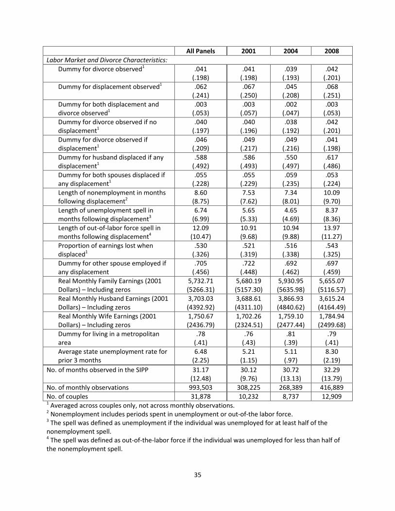
The last set of statistics in Table 1 summarizes the divorce and displacement events, the main

variables of interest, in the sample. On average, couples are observed for approximately 31 months.

During this period, a little over four percent of the couples in this sample divorce and about six percent

of couples experience a displacement. If no displacement occurs, about four percent of couples in this

12 The SIPP does collect information on assets but only in two or three surveys per panel, whereas investment income is collected in every survey.

17

sample are observed to divorce. If a displacement occurs, the proportion of those divorcing rises to 4.6

percent. Chi-square tests show that these proportions do not differ significantly.

Many of the displacement-related variables in Table 1 confirm the general recession trends

observed elsewhere. For example, the percentage of couples who experience a displacement is lowest

in the 2004 Panel, 4.5 percent, and highest in the 2008 Panel, 6.8%. Furthermore, many studies have

reported that the Great Recession affected males disproportionately compared with previous

recessions. The statistics in Table 1 confirm this finding since in the 2008 Panel, husbands were

displaced in about two-thirds of couples who experienced any displacement. Finally, the length of the

observed nonemployment spell following displacement is significantly greater in the 2008 Panel, as

expected. This result holds whether these spells were spent in predominantly in unemployment or out-

of-the-labor force (OLF).

The descriptive statistics in Table 1 capture many of the important trends of the Great Recession

- higher rates of displacement especially for men, longer unemployment spells, and lower home

ownership rates. In addition, the simple means suggest that divorce rates may be higher for those that

are displaced, in at least some years. In the next section, I will examine the relationship between these

variables and the probability of divorce in a statistical framework which controls for differences across

couples.

Section 6: Results

In the results presented in section 6.1, I control for match quality in equation (4) using a rich set

of covariates, similar to Charles and Stephens (2004), but do not attempt to control for any portion of

the match-specific component that is unobserved. In the robustness checks presented in section 6.2, I

assess how the results change with the changes to the definition of job loss and discuss controls for

unobserved heterogeneity.

18

6.1 Main Results

Table 2 shows results from estimating a basic hazard probit model of divorce with only

demographic covariates and no displacement controls. Both models (1) and (2) contain a rich set of

covariates that correspond to theory or past research. They also include fully-saturated interactions

between race and education covariates as well as controls for state-specific time-invariant effects, year-

month time effects, and state-specific linear time trends (these are not reported but available from the

author). Model (1) leaves out the effect of spousal earnings on the probability of divorce while model

(2) includes them. Since earnings may be confounded with the outcome of interest, displacement, I

leave earnings out of subsequent estimations that include displacement variables. Results are not

sensitive to the exclusion of earnings variables.

The results in Table 2 show that this basic model of divorce conforms well to theoretical

predictions. The duration dependence in marriage is captured through the use of cubic splines with

nodes at 3, 5, 7, 10, 15, 20, 25, and 30 years of marriage. The estimated coefficients on these splines

reflect a complex pattern of duration dependence with the divorce hazard peaking between 5 to 7

years, and again around 15 to 20 years of marriage after controlling for differences in observables.

The model results reveal that marital-specific investments, such as the number of children and

owning a house tend to significantly decrease the probability of divorce, although the effect of

investment income (a proxy for financial assets) while negative is insignificant. Unlike previous research,

the effect of children on the probability of divorce is allowed to vary by whether the children in the

household belong to both spouses biologically or only one. If the children belong to both spouses’

biologically (or are adopted), having more children is associated with a significantly lower probability of

divorce as evidenced by the negative coefficient on totalkids13. The coefficients on the quadratic

13 The variable totalkids includes the total number of both biological children and step-children living in the household, but because the variable stepkids is also included in the model, the variable totalkids essentially isolates the effect of biological children on the probability of divorce.

19

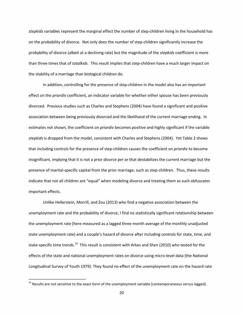
stepkids variables represent the marginal effect the number of step-children living in the household has

on the probability of divorce. Not only does the number of step-children significantly increase the

probability of divorce (albeit at a declining rate) but the magnitude of the stepkids coefficient is more

than three times that of totalkids. This result implies that step-children have a much larger impact on

the stability of a marriage than biological children do.

In addition, controlling for the presence of step-children in the model also has an important

effect on the priordiv coefficient, an indicator variable for whether either spouse has been previously

divorced. Previous studies such as Charles and Stephens (2004) have found a significant and positive

association between being previously divorced and the likelihood of the current marriage ending. In

estimates not shown, the coefficient on priordiv becomes positive and highly significant if the variable

stepkids is dropped from the model, consistent with Charles and Stephens (2004). Yet Table 2 shows

that including controls for the presence of step-children causes the coefficient on priordiv to become

insignificant, implying that it is not a prior divorce per se that destabilizes the current marriage but the

presence of marital-specific capital from the prior marriage, such as step-children. Thus, these results

indicate that not all children are “equal” when modeling divorce and treating them as such obfuscates

important effects.

Unlike Hellerstein, Morrill, and Zou (2013) who find a negative association between the

unemployment rate and the probability of divorce, I find no statistically significant relationship between

the unemployment rate (here measured as a lagged three month average of the monthly unadjusted

state unemployment rate) and a couple’s hazard of divorce after including controls for state, time, and

state-specific time trends.14 This result is consistent with Arkes and Shen (2010) who tested for the

effects of the state and national unemployment rates on divorce using micro-level data (the National

Longitudinal Survey of Youth 1979). They found no effect of the unemployment rate on the hazard rate

14 Results are not sensitive to the exact form of the unemployment variable (contemporaneous versus lagged).

20

of divorce for most marriages. These conflicting results suggest further research would be useful in

understanding the discrepancies.

In equation (2) in section 3, the gains from marriage depend upon both the husband’s and wife’s

income. To approximate income, model (2) in Table (2) includes quadratic specifications of each

spouse’s earnings and an interaction term between the two. This specification is similar to that used in

Weiss and Willis (1997) except that they used predicted earnings at the time of marriage instead of

actual earnings. The coefficients on the husband’s earnings variables suggest that all else equal,

increasing earnings reduce the probability of divorce though not significantly. The opposite is true for

the wife’s earnings – as her earnings increase, the probability of divorce increase. These results are

similar in sign to what Weiss and Willis found using predicted earnings. While they found a positive

interaction between the wife and husband’s predicted earnings, I find a negative though insignificant

effect suggesting the spouse’s earnings influence the divorce probability independently of each other.

6.1.1 Displacement – One Spouse versus Both Spouses

The first model in Table 3 includes all of the basic demographic and control variables from

model (1) in Table 2, but also adds the absorbing displacement indicator variable from the period in

which the spouse loses his/her job due to displacement (as opposed to quitting or being fired). The

coefficient on displaced indicates that displacement to one or both spouses significantly increases the

probability of divorce. In model (2), I also include the earnings variables from model (2) of Table 2 to

ensure that the displaced coefficient is not simply reflecting a correlation with the earnings variables. In

fact, this appears not to be the case, since the coefficient on displaced is still positive and significant.

Because the actual earnings variables do not appear to influence the displacement coefficient, I drop

these variables from the remainder of the analysis in order to focus on varying the job displacement

specification.

21

In the first two models of Table 3, the displacement variable captures the effect if either spouse

is displaced. However, it could be that the effect on the probability of divorce differs depending upon

whether one or both spouses’ lose their jobs. Theory suggests that although the utility of the current

marriage would fall so would the utilities of both spouses in the divorced state. Although the effect that

dominates is still theoretically ambiguous, it seems likely that divorce would be less likely to occur when

both spouses lose their jobs since it would be more difficult to finance the costs of divorce. To test for

these effects, model (3) interacts the displacement variables with an indicator variable identifying

couples in which both couples experience displacement. The result of the interaction suggests that

couples in which both spouses lose their jobs are less likely to divorce than couples in which only one

spouse is displaced, though the difference is not significant.

For the remainder of the analysis, I exclude couples in which both spouses are displaced (about

five percent of all couples who experienced any displacement) in order to focus on how other

circumstances, such as the sex of the job loser, affect the risk of divorce. The first model in Table 4

estimates the original displacement model in Table 3 (model (1)) on the reduced sample of 31,196

couples. Consistent with the previous results, the coefficient on displaced confirms that the job loss of

only one spouse significantly increases the divorce hazard. Indeed, calculating the average partial effect

of the displaced coefficient indicates that displacement increases the average predicted probability of

divorce by half of a percentage point annually. Because the baseline predicted probability of divorce is

relatively low, the effect of displacement translates into a 37% increase in the predicted probability of

divorce, all else held equal.

In the second model of Table (4), the effect of displacement on the probability of divorce is

allowed to vary by the sex of the job loser.15 The estimated coefficients reveal that only when the

husband is the spouse displaced does the probability of divorce significantly increase. Moreover, the

15 The coefficient displaced*wife is interpreted as the effect on the divorce risk when the wife is the spouse that is displaced. Likewise, displaced*husband represents the effect on the divorce risk when the husband is displaced.

22

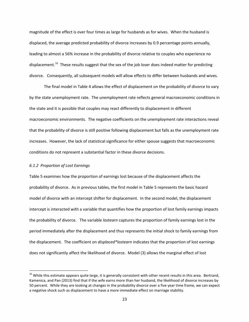
magnitude of the effect is over four times as large for husbands as for wives. When the husband is

displaced, the average predicted probability of divorce increases by 0.9 percentage points annually,

leading to almost a 56% increase in the probability of divorce relative to couples who experience no

displacement.16 These results suggest that the sex of the job loser does indeed matter for predicting

divorce. Consequently, all subsequent models will allow effects to differ between husbands and wives.

The final model in Table 4 allows the effect of displacement on the probability of divorce to vary

by the state unemployment rate. The unemployment rate reflects general macroeconomic conditions in

the state and it is possible that couples may react differently to displacement in different

macroeconomic environments. The negative coefficients on the unemployment rate interactions reveal

that the probability of divorce is still positive following displacement but falls as the unemployment rate

increases. However, the lack of statistical significance for either spouse suggests that macroeconomic

conditions do not represent a substantial factor in these divorce decisions.

6.1.2 Proportion of Lost Earnings

Table 5 examines how the proportion of earnings lost because of the displacement affects the

probability of divorce. As in previous tables, the first model in Table 5 represents the basic hazard

model of divorce with an intercept shifter for displacement. In the second model, the displacement

intercept is interacted with a variable that quantifies how the proportion of lost family earnings impacts

the probability of divorce. The variable lostearn captures the proportion of family earnings lost in the

period immediately after the displacement and thus represents the initial shock to family earnings from

the displacement. The coefficient on displaced*lostearn indicates that the proportion of lost earnings

does not significantly affect the likelihood of divorce. Model (3) allows the marginal effect of lost

16 While this estimate appears quite large, it is generally consistent with other recent results in this area. Bertrand, Kamenica, and Pan (2013) find that if the wife earns more than her husband, the likelihood of divorce increases by 50 percent. While they are looking at changes in the probability divorce over a five year time frame, we can expect a negative shock such as displacement to have a more immediate effect on marriage stability.

23

earnings to vary by the sex of the job loser. Here again, though, there seems to be no significant

additional effect of the proportion of lost earnings on the divorce probability.

In Table 5, the proportion of lost earnings was modeled linearly. It may be that the proportion

of lost earnings affects the divorce hazard nonlinearly. Consequently, in Table 6, models (2) and (3)

allow the effect of lost earnings on divorce to vary depending upon whether the proportion of earnings

lost falls into one of four categories: minor loss (0 to 0.40 of family earnings), equal loss (0.40 to 0.60),

major loss (0.60 to 0.99) or complete loss (1.00, i.e., the sole earner loses his or her job). The results

from model (3) in Table 6 reveal that the proportion of lost earnings does impact the divorce hazard

nonlinearly by the sex of the displaced spouse. The probability of divorce significantly increases when

the husband is displaced and the proportion of earnings lost is approximately one-half. Thus, Table 6

suggests that not only does the sex of the job loser matter in predicting divorce but the earning

structure of the marriage prior to divorce. Marriages most at risk of divorce following displacement

appear to be ones in which both spouses contributed somewhat equally to the financial resources of the

household.

6.1.3 Employment Characteristics of the Other Spouse

Previous specifications have examined how characteristics of the displaced spouse or the displacement

itself affect the probability of divorce. The specifications in this section consider the employment status

and earnings of the spouse who was not displaced. The findings from these models contribute to a

further understanding of how displacement may affect marital dissolution.

Table 7 explores how the employment status of the non-displaced spouse affects the probability

of divorce. As in previous tables, the first model in Table 7 specifies results for the basic displacement

model for comparison. In the second model, the marginal effect of displacement is allowed to vary by

whether the non-displaced spouse is employed or not (i.e., the variable spouse_employed equals one if

the non-displaced spouse is employed and zero otherwise). The estimated coefficient on the interaction

24

term displaced*spouse_employed indicates that the probability of divorce is not significantly higher

when the non-displaced spouse is employed than when he/she is not. However, the total effect on

divorce (displaced + displaced*spouse_employed) is statistically significant at the one percent level

implying that the risk of divorce increases for couples in which the non-displaced spouse is employed

relative to couples who do not experience displacement . Model (3) of Table 7 shows that the effect is

driven entirely by the displacement of husbands since the total effect when the wife is displaced is not

significant different that couples who experience no displacement.

Table 8 consists of a similar analysis to Table 7 except that these specifications examine the

effect of the non-displaced spouse’s earnings on the probability of divorce instead of simply whether or

not the non-displaced spouse was employed. These results are analogous to those found in the

previous table. The probability of divorce significantly increases with the non-displaced spouse’s

earnings but only when the displaced spouse is the husband. This result is highly robust to changes in

specification in addition to the the sample as will be seen in section 6.2.

6.1.4 Duration of the Unemployment Spell

As has been widely documented, the Great Recession was not only characterized by widespread

unemployment but also unemployment spells of unusually long duration. It is natural to wonder how

these longer spells affect the risk of marital dissolution. To investigate this issue, I define the period

between displacement and subsequent employment as a nonemployment spell. If I do not observe

subsequent employment, then the individual remains nonemployed until the last period of observation.

I then classify this spell as unemployment if the respondent spent the majority of periods looking for

work and OLF otherwise.17

17 I experimented with other rules for separating spells into unemployment and OLF but did not find results sensitive to the rule used.

25

The first column in Table 9 suggests that the marginal effect of an extra month of

nonemployment on the probability of divorce is not statistically significant. However, it may be that

effects on divorce differ depending upon whether the spouse spent the spell looking for work versus

being OLF. Therefore, model (2) allows this effect to vary depending upon the type of spell. The results

from model (2) suggest that the risk of divorce is not sensitive to whether the spouse spent the majority

of the spell unemployed or OLF. Additionally, when these results are allowed to vary by the sex of the

displaced spouse as in model (3), we find that an extra month spent in unemployment or OLF increases

the probability of divorce but only when the husband is displaced. Somewhat surprisingly, the

distinction between unemployment and OLF does not appear meaningful for displaced husbands as the

difference between the two coefficients is not statistically significant.

A fairly consistent pattern emerges from this and the previous set of analyses. Namely, that

divorces are more likely to occur when husbands rather than wives are the displaced spouse. Moreover,

the marriages most at risk of divorce appear to be those in which the wives are not only employed but a

relatively equal wage earner prior to displacement. Finally, both the wife’s earnings and the length of

the husband’s nonemployment spell appear to significantly increase the divorce hazard.

This study most closely resembles those by Charles and Stephens (2004) and Doiron and

Mendolia (2011). In their studies, they examine the effect of different types of job loss, including

displacements (or redundancies in the Doiron and Mendolia study) and terminations, on the probability

of divorce. While they find that terminations or firings increase the divorce hazard, they find no

significant effect for displacements. In contrast, I focus solely on displacements and find positive

significant effects on the divorce hazard under certain circumstances. My more nuanced finding could

reflect the more recent trends both in marital formation, female labor force participation, and job loss

compared to the 1968-93 period studied by Charles and Stephens (2004). In comparing my results with

26

Doiron and Mendolia, it is difficult to assess how including cohabiting couples in their analysis affects

their results.

6.2 Robustness Analysis

While I have limited the definition of job loss to reasons that I believe are exogenous to the

qualities and performance of the individual (“employer bankrupt, employer sold business, slack work or

business conditions”) it may be that some of these reasons do not reflect true displacement, especially if

the individuals displaced under “slack work or business conditions” were less productive than their

retained counterparts. When Charles and Stephens (2004) limited their definition of job loss to plant

closings and bankruptcy (events they assumed to be truly exogenous to the individual), they found that

there was no significant impact of job loss on the divorce hazard for either spouse. To test the

robustness of the results presented in section 6.1, in this analysis I similarly restrict job loss to only

reasons of “employer bankrupt” and “employer sold business.”

Table 10 presents results using this more restrictive definition. Limiting job loss to only

“employer bankrupt” and “employer sold business” reduces the proportion of the sample experiencing

a displacement substantially from 5.6 percent to 0.42 percent. The results in model (1) and (2) suggest

that, as in Charles and Stephens (2004), displacement does not significantly affect the divorce hazard

even when allowing for differential effects by sex of the displaced spouse. However, whereas Charles

and Stephens found a negative effect of plant closings on divorce for men, I find a positive effect,

consistent with the previous results found in section 6.1.

Unfortunately, the reduced sample size of couples experiencing displacement under the more

restrictive definition prevents estimation of many of the models in the previous section. However,

model (3) attempts to reproduce the analysis in column (3) of Table 8, specifically estimating how the

earnings of the non-displaced spouse affect the probability of divorce. The positive significant

coefficient on displaced*spouse_earn*husband support previous results showing the divorce

27

significantly increases with the wife’s earnings when her husband is displaced. While it would be nice to

test the robustness of more of the previous results, this finding confirms that it was not a broader

definition of displacement that was driving the highly significant, positive effect of spousal earnings on

divorce.

Another assessment of the robustness of the main results involves controlling for couple i’s

unobserved match characteristic µi. As discussed in the estimation section, the unobserved match

characteristic can be integrated out of the likelihood function using random effects yielding consistent

coefficients (Wooldridge 2010).18 Tables 11 and 12 re-estimate relevant probit models from section 6.1

but control for random effects.19 Table 11 shows the results of re-estimating models (1) and (2) from

Table 4 (which include intercept shifters for any displacement and displacement by sex of the displaced

spouse), and model (3) from Table 9 (which allows the probability of divorce to vary by the duration of

the husband’s unemployment or OLF spell). The sign and significance of the coefficients in Table 11 are

consistent with those previously estimated suggesting that while unobserved heterogeneity is present,

according to the likelihood ratio test that rho=0, it does not affect the main results. Table 12 reproduces

estimations from model (3) of Table 6 (which allows the probability of divorce to vary non-linearly by the

proportion of earnings lost from displacement) and model (3) of Table 8 (which allows the probability of

divorce to vary by the earnings of the non-displaced spouse). The results in model (2) of Table 12 reveal

that while the effect on the divorce risk is still positive when husbands are displaced who contributed

approximately half the family’s earnings prior to displacement, this result is no longer statistically

significant as it was in Table 6. However, model (3) in Table 12 confirms the robustness of the finding

18 There are two other ways to control for the unobserved heterogeneity across couples: discrete-choice fixed effects estimators and random or fixed effects in the linear probability model. However, the combination of the large sample size (n > 31,000 couples) and the low frequency outcome of the divorce dependent variable (with no variation in the panel for couples who do not divorce) render these estimators unfeasible for this application. 19 Although I would have preferred to re-estimate the exact specifications in section 6.1 but controlling for random effects, that was not always possible due to difficulties with convergence. While all of the models in Tables 11 and 12 control for the base variables and state and month-year effects, I have dropped the state-linear time trend interactions. In addition, in some models I have had to limit the displacement-related interactions to the most relevant variables.

28

the husband’s displacement increases the probability of divorce as the wife’s earnings increase since this

coefficient (displaced*spouse_earn_husband) remains positive and significant at the 1 percent level.

In sum, the pattern of results appears fairly similar between the models that do and do not

control for unobserved heterogeneity. Overall, this analysis suggests that ignoring unobserved

heterogeneity in estimation in section 6.1 does not appear to be driving this study’s main results.

Section 7: Discussion of Results

This study points to several interesting findings and areas for further research. First, this study finds that

there is an asymmetry in the way job loss is viewed within the marriage. Whereas a wife’s displacement

appears to have no significant effect on the probability of divorce, a husband’s job loss can destabilize

the marriage when the wife is also employed and as her earnings increase. This results suggests that at

least for some marriages, the husband’s earning capacity is still of primary importance in the gains to

being married. When this ability falls, even through no fault of his own, the marriage is more likely to

dissolve. This result is consistent with a theory of gender identity and relative income posited by

Bertrand, Kamenica, and Pan (2013) in which couples have an aversion to the wife earning more than

the husband. The authors find that when the wife earns more than the husband (a departure from

traditional gender roles) the likelihood of divorce substantially increases.

A separate but related reason for the observed gender asymmetries may be that women are

better than men at substituting home production for market production when displaced. If this is true,

then we would expect the gains to marriage to fall less when wives rather than husbands are displaced

and thus would expect to observe fewer divorces.

Second, previous studies such as Charles and Stephens (2004) and Doiron and Mendolia (2011)

have suggested that their positive, significant results for terminations/layoffs versus displacements on

the probability of divorce is due to the negative signal that terminations provide regarding a spouse’s

suitability and future earning capacity. While this may be true, this study finds that job losses may have

29

significant effects on the probability of divorce even when they are exogenous to the individual. It

seems unlikely that this type of exogenous displacement would signal an underlying unsuitability.

Rather, it may be that some spouses realize that job losses can affect future earning capacity even when

exogenous. For example, studies such as Davis and von Wachter (2011) and Couch and Placzek (2010)

find that displacements lower future earnings, especially when they occur during recessions.

Consequently, the displacement need not be a signal of underlying match suitability to affect expected

future earnings and thus the probability of divorce.

Finally, given the negative economic and societal consequences of divorce, it would be

interesting to know whether unemployment-related policies, such as unemployment benefits or

retraining programs, have any effects on the probability of divorce by ameliorating the effects of

displacement on the family. Research in this area would help shed light on the relative importance of

gender roles versus policy intervention in marital dissolution decisions.

30

REFERENCES

Amato, Paul R. 2000. “The Consequences of Divorce for Adults and Children.” Journal of Marriage and Family 62 (4):1269-1287.

Arkes, Jeremy and Yu-Chu Shen. 2010. “For Better or For Worse, But How About a Recession?” NBER Working Paper 16525.

Becker, Gary S. 1974. “A Theory of Marriage” in Economics of the Family. Edited by T. W. Schultz. Chicago, IL: University of Chicago Press.

Becker, Gary S., Elisabeth M. Landes, and Robert T. Michael. 1977. “An Economic Analysis of Marital Instability.” Journal of Political Economy 85(6):1141-1187.

Bertrand, Marianne, Emir Kamenica, and Jessica Pan. 2013. “Gender identity and relative income within households.” Natural Bureau of Economic Research Working Paper No. 19023.

Biblarz, Timothy J. and Greg Gottainer. 2004. “Family Structure and Children’s Success: A Comparison of Widowed and Divorced Single-Mother Families.” Journal of Marriage and the Family 62(2):533–548.

Bredemeier, Christian and Falko Juessen. 2013. “Assortative Mating and Female Labor Supply.” Journal of Labor Economics 31(3):603-631.

Charles, Kerwin Kofi, and Melvin Stephens, Jr. 2004. “Job Displacement, Disability, and Divorce.” Journal of Labor Economics 22(2):489-522.

Corak, Miles. 2001 “Death and Divorce: The Long-Term Consequences of Parental Loss on Adolescents.” Journal of Labor Economic 19(3): 682-715.

Couch, Kenneth A. and Dana W. Placzek. 2010. “Earnings Losses of Displaced Workers Revisited.” American Economic Review 100(1):572-589.

Davis, Steven J. and Till von Wachter. 2011. “Recessions and the Costs of Job Loss.” Brookings Papers on Economic Activity (Fall).

Doiron, Denise and Silvia Mendolia. 2011. “The Impact of Job on Family Dissolution.” Journal of Population Economics 25(1):367-398.

Farnham, Martin, Lucie Schmidt, and Purvi Sevak. 2011. “House Prices and Marital Stability.” American Economic Review: Papers and Proceedings 101(3):615-619.

Guo, Guang. 1993. “Event-History Analysis for Left-Truncated Data.” Sociological Methodology 23:217-243.

Gruber, Jonathan. 2004. “Is Making Divorce Easier Bad for Children? The Long-Run Implications of Unilateral Divorce.” Journal of Labor Economics 22(4):799-833.

31

Hankins, Scott and Mark Hoekstra. 2011. “Lucky in Life, Unlucky in Love? The Effect of Random Income Shocks on Marriage and Divorce.” Journal of Human Resources 46(2):403-426.

Hellerstein, Judith K. and Melinda Sandler Morrill. 2011. “Booms, Busts, and Divorce.” The B.E. Journal of Economic Analysis and Policy 11(1), Article 54.

Hellerstein, Judith K., Melinda Sandler Morrill, and Ben Zou. 2013. “Business Cycles and Divorce: Evidence from Microdata.” Economic Letters 188(January):68-70.

Isen, Adam and Betsey Stevenson. 2011. “Women’s Education and Family Behavior: Trends in Marriage, Divorce, and Fertility” in Demography and the Economy. Edited by John B. Shoven. Chicago, IL: The University of Chicago Press.

Kane, John, Lawrence M. Spizman, James Rodgers and Rick R. Gaskins. 2010. “The Effect of the Loss of a Parent on the Future Earnings of a Minor Child.” Eastern Economic Journal 36:370–390.

Lundberg, Shelly. 2012. “Personality and marital surplus.” IZA Journal of Labor Economics 1:3.

Page, Marianne E. and Ann Huff Stevens. 2004 “The Economic Consequences of Absent Parents.” Journal of Human Resources 39(1):80-107.

Painter, Gary and David I. Levine. 2000. "Family Structure and Youths' Outcomes: Which Correlations Are Causal?" Journal of Human Resources 35(3):524-49.

Singleton, Perry. 2012. “Insult to Injury: Disability, Earnings, and Divorce.” Journal of Human Resources 47(4):972-990.

Stevenson, Betsey and Justin Wolfers. 2007. “Marriage and Divorce: Changes and Their Driving Forces.” Journal of Economic Perspectives 21(2):27-52.

Tartari, Melissa. 2007. “Divorce and the Cognitive Achievement of Children.” Unpublished manuscript, Yale University.

Weiss, Yoram, and Robert J. Willis. 1997. “Match Quality, New Information, and Martial Dissolution.” Journal of Labor Economics 15(1, pt. 2):S293-S329.

Wooldridge, Jeffrey M. 2010. Econometric Analysis of Cross Section and Panel Data. Cambridge, MA: The MIT Press.

32

Figure 1 – Annual Divorce Hazard Conditional on Marriage Duration

0.0

05.0

1.0

15.0

2.0

25A

nnua

l Div

orce

Haz

ard

0 5 10 15 20 25 30 35Marriage Duration in Years

Annual Divorce Hazard (Weighted)

33

Table 1 – Means of Selected Characteristics for Married Couples in Sample (statistics are weighted; standard deviations in parentheses) All Panels 2001 2004 2008 Match Characteristics of Couple:

Husband’s age when current marriage began1

28.87 (7.94)

28.54 (7.87)

28.68 (7.83)

29.29 (8.05)

Wife’s age when current marriage began1

26.77 (7.56)

26.38 (7.48)

26.63 (7.50)

27.20 (7.64)

Dummy for age difference greater than 10 years between spouses1

.06 (.24)

.06 (.24)

.06 (.24)

.06 (.24)

Dummy for first marriage1 .67 (.47)

.66 (.47)

.67 (.47)

.68 (.47)

Dummy for same race1 .92 (.27)

.94 (.24)

.92 (.27)

.92 (.28)

Dummy for both white, non-hispanic1 .73 (.45)

.76 (.43)

.72 (.45)

.70 (.46)

Dummy for both black, non-hispanic1 .06 (.24)

.06 (.24)

.06 (.24)

.06 (.23)

Dummy for same education level: .60 (.49)

.60 (.49)

.59 (.49)

.60 (.49)

Both high school grads or less .21 (.41)

.26 (.44)

.19 (.39)

.19 (.39)

Both some college .16 (.36)

.14 (.35)

.18 (.38)

.16 (.37)

Both college grads. .23 (.42)

.21 (.41)

.22 (.42)

.25 (.44)

Marital Investments: Marriage duration 17.12

(11.22) 16.55

(11.08) 17.13

(11.04) 17.55

(11.41) Dummy for any children .67

(.47) .67

(.47) .68

(.47) .65

(.48) Total number of children in household, if any

2.01 (1.02)

1.99 (1.00)

2.03 (1.02)

2.01 (1.03)

Dummy for either spouse previously divorced1

.32 (.47)

.33 (.47)

.32 (.47)

.31 (.46)

Dummy for couples with any step-children in household

.08 (.27)

.07 (.26)

.09 (.29)

.08 (.28)

Total number of step-children, if any 1.50 (.79)

1.51 (.83)

1.50 (.78)

1.48 (.75)

Dummy for owning home .84 (.37)

.84 (.37)

.85 (.36)

.83 (.38)

Dummy for any investment income .69 (.46)

.69 (.46)

.71 (.45)

.69 (.46)

Real Monthly Investment income (2001 Dollars), if any

99.29 (361.87)

116.80 (437.30)

102.51 (327.97)

82.87 (309.40)

34

All Panels 2001 2004 2008 Labor Market and Divorce Characteristics:

Dummy for divorce observed1 .041 (.198)

.041 (.198)

.039 (.193)

.042 (.201)

Dummy for displacement observed1 .062 (.241)

.067 (.250)

.045 (.208)

.068 (.251)

Dummy for both displacement and divorce observed1

.003 (.053)

.003 (.057)

.002 (.047)

.003 (.053)

Dummy for divorce observed if no displacement1

.040 (.197)

.040 (.196)

.038 (.192)

.042 (.201)

Dummy for divorce observed if displacement1

.046 (.209)

.049 (.217)

.049 (.216)

.041 (.198)

Dummy for husband displaced if any displacement1

.588 (.492)

.586 (.493)

.550 (.497)

.617 (.486)

Dummy for both spouses displaced if any displacement1

.055 (.228)

.055 (.229)

.059 (.235)

.053 (.224)

Length of nonemployment in months following displacement2

8.60 (8.75)

7.53 (7.62)

7.34 (8.01)

10.09 (9.70)

Length of unemployment spell in months following displacement3

6.74 (6.99)

5.65 (5.33)

4.65 (4.69)

8.37 (8.36)

Length of out-of-labor force spell in months following displacement4

12.09 (10.47)

10.91 (9.68)

10.94 (9.88)

13.97 (11.27)

Proportion of earnings lost when displaced1

.530 (.326)

.521 (.319)

.516 (.338)

.543 (.325)

Dummy for other spouse employed if any displacement

.705 (.456)

.722 (.448)

.692 (.462)

.697 (.459)

Real Monthly Family Earnings (2001 Dollars) – Including zeros

5,732.71 (5266.31)

5,680.19 (5157.30)

5,930.95 (5635.98)

5,655.07 (5116.57)

Real Monthly Husband Earnings (2001 Dollars) – Including zeros

3,703.03 (4392.92)

3,688.61 (4311.10)

3,866.93 (4840.62)

3,615.24 (4164.49)

Real Monthly Wife Earnings (2001 Dollars) – Including zeros

1,750.67 (2436.79)

1,702.26 (2324.51)

1,759.10 (2477.44)

1,784.94 (2499.68)

Dummy for living in a metropolitan area

.78 (.41)

.76 (.43)

.81 (.39)

.79 (.41)

Average state unemployment rate for prior 3 months

6.48 (2.25)

5.21 (1.15)

5.11 (.97)

8.30 (2.19)

No. of months observed in the SIPP 31.17 (12.48)

30.12 (9.76)

30.72 (13.13)

32.29 (13.79)

No. of monthly observations 993,503 308,225 268,389 416,889 No. of couples 31,878 10,232 8,737 12,909 1 Averaged across couples only, not across monthly observations. 2 Nonemployment includes periods spent in unemployment or out-of-the labor force. 3 The spell was defined as unemployment if the individual was unemployed for at least half of the nonemployment spell. 4 The spell was defined as out-of-the-labor force if the individual was unemployed for less than half of the nonemployment spell.

35

Table 2. Discrete-time hazard model (probit) of divorce – Base models ignoring displacement (standard errors are clustered by couple) (1) (2) Base Model (no

displacement variables, no

earnings)

Base Model (no displacement

variables, with earnings)

Marriage Duration spline: 3 - 5 years 0.0919* 0.0912* (0.0381) (0.0381) 5 - 7 years 0.106** 0.105** (0.0402) (0.0402) 7 - 10 years 0.0668 0.0663 (0.0397) (0.0397) 10 - 15 years 0.0972* 0.0976* (0.0394) (0.0393) 15 - 20 years 0.153** 0.153** (0.0429) (0.0429) 20 - 25 years 0.0527 0.0524 (0.0467) (0.0467) 25 - 30 years -0.104* -0.105* (0.0498) (0.0499) 30 - 50 years -0.468** -0.465** (0.0531) (0.0533) priordiv -Dummy for any prior divorce -0.0354 -0.0355 (0.0268) (0.0268) totalkids - No. of children in household -0.151** -0.149** (0.0143) (0.0144) totalkids0_5 - No. of children, age 0 to 5, in household 0.0446* 0.0486* (0.0196) (0.0196) stepkids - No. of step-children in household 0.564** 0.562** (0.0333) (0.0333) stepkids2 -0.0519** -0.0517** (0.00818) (0.00818) ownhome - Dummy for own home -0.180** -0.186** (0.0222) (0.0227) assetinc -Total dividend/interest income (real $, per 1000) -0.125 -0.129 (0.0811) (0.0821) assetinc2 0.00756 0.00781 (0.00517) (0.00522) agediff10 – Dummy for age difference between spouses greater than 0.0482 0.0484 10 years (0.0329) (0.0329) agemarr_w - Age at marriage for wife -0.0159** -0.0159** (0.00182) (0.00183) earn_h -Husband’s real earnings (per $1,000) -0.00650 (0.00412) earn_h2 0.000259** (6.59e-05) earn_w - Wife’s real earnings (per $1,000) 0.0218*

36

(0.00916) earn_w2 -0.00114 (0.000670) earn_h*earn_w -1.89e-05 (0.000772) metro – Dummy for residing in metropolitan area 0.00635 0.00516 (0.0239) (0.0239) unemp_rate – Avg. state unemployment rate for prior 3 months 0.0132 0.0134 (0.0167) (0.0167) constant -3.355** -3.353** (0.296) (0.296) Full education interactions between spouses Yes Yes Full racial interactions between spouses Yes Yes State dummies Yes Yes Month-year dummies Yes Yes Linear state time trend Yes Yes No. of couple-month observations 992,539 992,539 No. of couples 31,850 31,850 Pseudo R-squared 0.1083 0.1089

Robust standard errors in parentheses ** p<0.01, * p<0.05

37

Table 3. Discrete-time hazard model (probit) of divorce – Includes displacement variables (includes base model variables and controls for state effects, month-year effects, and linear state-time trend; standard errors are clustered by couple) (1) (2) (3) Displacement –

one spouse, no earnings

Displacement – one spouse,

with earnings

Displacement – both spouses

displaced 0.0972** 0.0982** 0.101** (0.0368) (0.0371) (0.0376) displaced*displaced_both -0.0742 (0.173) Includes earnings variables No Yes No No. of couple-month observations 992,539 992,539 992,539 No. of couples 31,850 31,850 31,850 Pseudo R-squared 0.1086 0.1092 0.1086

Robust standard errors in parentheses ** p<0.01, * p<0.05

38

Table 4. Discrete-time hazard model (probit) of divorce – displacement variable interacted with sex of laid-off spouse and the unemployment rate (includes base model variables and controls for state effects, month-year effects, and linear state-time trend; standard errors are clustered by couple) (1) (2) (3) No spouse or

unemployment rate interactions

Spouse interactions

Spouse and unemploy. rate

interactions displaced 0.105** (0.0391) displaced*wife 0.0355 0.0821 (0.0638) (0.178) displaced*wife*unemp_rate -0.00667 (0.0242) displaced*husband 0.150** 0.307* (0.0480) (0.149) displaced*husband*unemp_rate -0.0219 (0.0198) No. of couple-month observations 970,011 970,011 970,011 No. of couples 31,196 31,196 31,196 Pseudo R-squared 0.1092 0.1093 0.1093

Robust standard errors in parentheses ** p<0.01, * p<0.05

39

Table 5. Discrete-time hazard model (probit) of divorce – displacement variable interacted with proportion of lost earnings and sex of laid-off spouse (includes base model variables and controls for state effects, month-year effects, and linear state-time trend; standard errors are clustered by couple) (1) (2) (3) Displacement

only Displacement & proportion of lost

earnings

Displacement & proportion of lost

earnings with spouse interactions

displaced 0.105** 0.132 (0.0391) (0.0749) displaced*lostearn -0.0534 (0.122) displaced*wife 0.0989 (0.106) displaced *wife*lostearn -0.183 (0.244) displaced*husband 0.233* (0.114) displaced *husband*lostearn -0.134 (0.168) No. of couple-month observations 970,011 970,011 970,011 No. of couples 31,196 31,196 31,196 Pseudo R-squared 0.1092 0.1092 0.1094

Robust standard errors in parentheses ** p<0.01, * p<0.05

40

Table 6. Discrete-time hazard model (probit) of divorce – displacement variable and proportion of lost earnings by group and sex of laid-off spouse (includes base model variables, weights and controls for state effects, month-year effects, and linear state-time trend; standard errors are clustered by couple) (1) (2) (3) Displacement

only Proportion of

lost earnings by group

Proportion of lost earnings by

group with spouse

interactions displaced 0.105** (0.0391) displaced*minor loss (0 to 0.33] 0.0917 (0.0617) displaced*minor loss*wife 0.0444 (0.0798) displaced*minor loss*husband 0.169 (0.0953) displaced*equal loss (0.33 to 0.66] 0.116 (0.0787) displaced*equal loss*wife -0.102 (0.165) displaced*equal loss*husband 0.204* (0.0895) displaced*major loss (0.66 to 0.99] 0.0800 (0.0973) displaced*major loss*wife 0.298 (0.248) displaced*major loss*husband 0.0409 (0.104) displaced*complete loss [1.00] 0.136 (0.0775) displaced*complete loss*wife 0.0589 (0.148) displaced*complete loss*husband 0.158 (0.0900) No. of couple-month observations 970,011 970,011 970,011 No. of couples 31,196 31,196 31,196 Pseudo R-squared 0.1092 0.1092 0.1095

Robust standard errors in parentheses ** p<0.01, * p<0.05

41

Table 7. Discrete-time hazard model (probit) of divorce – displacement variable, employment status of spouse and unemployment rate interactions (includes base model variables and controls for state effects, month-year effects, and linear state-time trend; standard errors are clustered by couple) (1) (2) (3) Displacement

only Spouse’s

employment status Spouse’s employment

status by sex displaced 0.105** 0.0244 (0.0391) (0.0765) displaced*spouse_employed 0.105 (0.0872) displaced*wife 0.000360 (0.150) displaced *wife 0.0406 *spouse_employed (0.164) displaced*husband 0.0317 (0.0885) displaced *husband 0.167 *spouse_employed (0.105) No. of couple-month observations

970,011 970,011 970,011

No. of couples 31,196 31,196 31,196 Pseudo R-squared 0.1092 0.1092 0.1094

Robust standard errors in parentheses ** p<0.01, * p<0.05

42

Table 8. Discrete-time hazard model (probit) of divorce – displacement variable, earnings of spouse and unemployment rate interactions (includes base model variables and controls for state effects, month-year effects, and linear state-time trend; standard errors are clustered by couple) (1) (2) (3) Displacement

only Spouse’s earnings Spouse’s earnings

by sex displaced 0.105** 0.0607 (0.0391) (0.0441) displaced*spouse_earn 0.0195* (0.00900) displaced*wife -0.0287 (0.0810) displaced*wife 0.0170 *spouse_earn (0.0142) displaced*husband 0.0856 (0.0548) displaced*husband 0.0440** *spouse_earn (0.0144) No. of couple-month observations 970,011 970,011 970,011 No. of couples 31,196 31,196 31,196 Pseudo R-squared 0.1092 0.1093 0.1102

Robust standard errors in parentheses ** p<0.01, * p<0.05

43

Table 9. Discrete-time hazard model (probit) of divorce – displacement variable and duration of nonemployment, unemployment, and out-of-labor force (OLF) spells (includes base model variables and controls for state effects, month-year effects, and linear state-time trend; standard errors are clustered by couple) (1) (2) (3) Duration of

nonemployment spell

Duration of unempl. and OLF spells

Duration of unempl. and OLF spells by

sex displaced 0.0425 0.0405 (0.0518) (0.0527) displaced*nonemp_spell 0.00978 (0.00521) displaced* OLF_spell 0.00930 (0.00596) displaced* unemp_spell 0.0108 (0.00721) displaced*wife 0.0635 (0.0797) displaced*wife*OLF_spell -0.00300 (0.00845) displaced*wife*unemp_spell* -0.00613 (0.0124)

displaced*husband 0.0327 (0.0679)

displaced*husband*OLF_spell 0.0198* (0.00775)

displaced*husband*unemp_spell* 0.0182* (0.00879) No. of couple-month observations 970,011 970,011 970,011 No. of couples 31,196 31,196 31,196 Pseudo R-squared 0.1093 0.1093 0.1097

Robust standard errors in parentheses ** p<0.01, * p<0.05

44

Table 10. Discrete-time hazard model (probit) of divorce – displacement due to “employer bankrupt” or “employer sold firm” only, with employment status and earnings of non-laid-off spouse (includes base model variables and controls for state effects, month-year effects, and linear state-time trend; standard errors are clustered by couple) (1) (2) (3) Displacement

only Spouse interactions Wife’s earnings

displaced 0.0347 (0.125) displaced*wife -0.300 -0.300 (0.286) (0.286) displaced*husband 0.185 -0.279 (0.146) (0.219) displaced*spouse_earn 0.168** *husband (0.0509) No. of couple-month observations 915,883 915,883 915,883 No. of couples 29,628 29,628 29,628 Pseudo R-squared 0.1098 0.1100 0.1103

Robust standard errors in parentheses ** p<0.01, * p<0.05

45

Table 11. Discrete-time hazard model (probit) of divorce controlling for random effects – displacement variable and duration of husband’s unemployment or out-of-labor-force (OLF) spells (includes base model variables, controls for state effects and month-year effects)

(1) (2) (3) Displacement

only Spouse

interactions Duration of husband’s

unemploy. and OLF spells

displaced 0.2186* (0.0981) displaced*wife 0.1021 .1047 (0.1531) (.1520) displaced*husband 0.3031* .0259 (0.1269) (.1611) displaced*husband*OLF_spell .0524** (.0192) displaced*husband*unemp_spell .0467* (.0216) ln(σ2

µ) 1.401 1.445 1.412 (0.039) (0.037) (0.039) σµ 2.022 2.060 2.025 (0.039) (0.039) (0.040) rho 0.8041 0.8091 0.8041 (0.006) (0.006) (0.006) No. of couple-month obs. 970,959 970,959 970,959 No. of couples 31,223 31,223 31,223 Notes: ** p<0.01, * p<0.05, 1 Likelihood-ratio test of rho=0, Probability (rho>= chibar2) = 0.000

46

Table 12. Discrete-time hazard model (probit) of divorce controlling for random effects – displacement variable, earnings of non-laid-off spouse and proportion of lost earnings (includes base model variables, controls for state effects and month-year effects)

(1) (2) (3) Displacement

only Proportion of lost earnings by group

with spouse interactions

Non-displaced spouse’s

earnings by sex

displaced 0.2186* 0.0554 (0.0981) (0.1194) Proportion of Earnings Lost displaced*minor loss* 0.1739 wife (0.1847) displaced*minor loss* 0.4414 husband (0.2353) displaced*equal loss* -0.2363 wife (0.3842) displaced*equal loss* 0.4399 husband (0.2424) displaced*major loss* 0.5146 wife (0.5757) displaced*major loss* 0.0214 husband (0.2738) displaced*complete loss* -0.0783 wife (0.4533) displaced*complete loss* 0.2262 husband (0.2440) Spouse’s earnings displaced*spouse_earn 0.0328 *wife (0.0289) displaced*spouse_earn 0.1121** *husband (0.0431) ln(σ2

µ) 1.401 1.383 1.421 (0.039) (0.040) (0.037) σµ 2.022 1.997 2.035 (0.039) (0.038) (0.037) rho 0.8041 0.8001 0.8061 (0.006) (0.006) (0.006) No. of couple-month obs. 970,959 970,959 970,959 No. of couples 31,223 31,223 31,223 Notes: ** p<0.01, * p<0.05, 1 Likelihood-ratio test of rho=0, Probability (rho>= chibar2) = 0.000

47