Embed Size (px)
Citation preview

When Inequality Matters for Macro
and Macro Matters for Inequality∗
SeHyoun Ahn Greg Kaplan Benjamin Moll
Thomas Winberry Christian Wolf
May 31, 2017
Abstract
We develop an efficient and easy-to-use computational method for solving a wideclass of general equilibrium heterogeneous agent models with aggregate shocks. Ourmethod extends standard linearization techniques and is designed to work in caseswhen inequality matters for the dynamics of macroeconomic aggregates. We presenttwo applications that analyze a two-asset incomplete markets model parameterized tomatch the distribution of income, wealth, and marginal propensities to consume. First,we show that our model is consistent with two key features of aggregate consumptiondynamics that are difficult to match with representative agent models: (i) the sensi-tivity of aggregate consumption to predictable changes in aggregate income and (ii)the relative smoothness of aggregate consumption. Second, we extend the model tofeature capital-skill complementarity and show how factor-specific productivity shocksshape dynamics of income and consumption inequality.
∗Ahn: Princeton University, e-mail [email protected], Kaplan: University of Chicago and NBER,e-mail [email protected]; Moll: Princeton University, CEPR and NBER, e-mail [email protected];Winberry: Chicago Booth and NBER, e-mail [email protected]; Wolf: Princeton Uni-versity, email [email protected]. We thank Chris Carroll, Chris Sims, Jonathan Parker, Bruce Pre-ston, Stephen Terry, and our discussant John Stachurski for useful comments. Paymon Khorrami providedexcellent research assistance.

1 Introduction
Over the last thirty years, tremendous progress has been made in developing models that
reproduce salient features of the rich heterogeneity in income, wealth, and consumption
behavior across households that is routinely observed in micro data. These heterogeneous
agent models often deliver strikingly different implications of monetary and fiscal policies
than do representative agent models, and allow us to study the distributional implications
of these policies across households.1 In principle, this class of models can therefore incorpo-
rate the rich interaction between inequality and the macroeconomy that characterizes our
world: on the one hand, inequality shapes macroeconomic aggregates; on the other hand,
macroeconomic shocks and policies affect inequality.
Despite providing a framework for thinking about these important issues, heterogeneous
agent models are not yet part of policy makers’ toolbox for evaluating the macroeconomic
and distributional consequences of their proposed policies. Instead, most quantitative anal-
yses of the macroeconomy, particularly in central banks and other policy institutions, still
employ representative agent models. Applied macroeconomists tend to make two excuses
for this abstraction. First, they argue that the computational difficulties involved in solving
and analyzing heterogeneous agent models render their use intractable, especially compared
to the ease with which they can analyze representative agent models using software pack-
ages like Dynare. Second, there is a perception among macroeconomists that models which
incorporate realistic heterogeneity are unnecessarily complicated because they generate only
limited additional explanatory power for aggregate phenomena. Part of this perception stems
from the seminal work of Krusell and Smith (1998), who found that the business cycle prop-
erties of aggregates in a baseline heterogeneous agent model are virtually indistinguishable
from those in the representative agent counterpart.2,3
Our paper’s main message is that both of these excuses are less valid than commonly
1For examples studying fiscal policy, see McKay and Reis (2013) and Kaplan and Violante (2014); formonetary policy, see McKay, Nakamura and Steinsson (2015), Auclert (2014), and Kaplan, Moll and Violante(2016).
2More precisely, in Krusell and Smith (1998)’s baseline model, which is a heterogenous agent version of astandard Real Business Cycle (RBC) model with inelastic labor supply, the effects of technology shocks onaggregate output, consumption and investment are indistinguishable from those in the RBC model.
3Lucas (2003) succinctly captures many macroeconomists’ view when he summarizes Krusell and Smith’sfindings as follows: “For determining the behavior of aggregates, they discovered, realistically modeledhousehold heterogeneity just does not matter very much. For individual behavior and welfare, of course,heterogeneity is everything.” Interestingly, there is a discrepancy between this perception and the results inKrusell and Smith (1998): they show that an extension of their baseline model with preference heterogeneity,thereby implying a more realistic wealth distribution, “features aggregate time series that depart significantlyfrom permanent income behavior.”
1

thought. To this end, we make two contributions. First, we develop an efficient and easy-to-
use computational method for solving a wide class of general equilibrium heterogeneous agent
macro models with aggregate shocks, thereby invalidating the first excuse. Importantly, our
method also applies in environments that violate what Krusell and Smith (1998) have termed
“approximate aggregation”, i.e. that macroeconomic aggregates can be well described using
only the mean of the wealth distribution.
Second, we use the method to analyze the time series behavior of a rich two-asset het-
erogeneous agent model parameterized to match the distribution of income, wealth, and
marginal propensities to consume (MPCs) in the micro data. We show that the model is
consistent with two features of the time-series of aggregate consumption that have proven to
be a challenge for representative agent models: consumption responds to predictable changes
in income but at the same time is substantially less volatile than realized income. We then
demonstrate how a quantitatively plausible heterogeneous agent economy such as ours can
be useful in understanding the distributional consequences of aggregate shocks, thus paving
the way for a complete analysis of the transmission of shocks to inequality. These results
invalidate the second excuse: not only does macro matter for inequality, but inequality also
matters for macro. We therefore view an important part of the future of macroeconomics
as the study of distributions – the representative-agent shortcut may both miss a large part
of the story (the distributional implications) and get the small remaining part wrong (the
implications for aggregates).
In Section 2, we introduce our computational methodology, which extends standard lin-
earization techniques, routinely used to solve representative agent models, to the heteroge-
neous agent context.4 For pedagogical reasons, we describe our methods in the context of
the Krusell and Smith (1998) model, but the methods are applicable much more broadly.
We first solve for the stationary equilibrium of the model without aggregate shocks (but with
idiosyncratic shocks) using a global non-linear approximation. We use the finite difference
method of Achdou et al. (2015) but, in principle, other methods can be used as well. This ap-
proximation gives a discretized representation of the model’s stationary equilibrium, which
includes a non-degenerate distribution of agents over their individual state variables. We
then compute a first-order Taylor expansion of the discretized model with aggregate shocks
around the stationary equilibrium. This results in a large, but linear, system of stochas-
tic differential equations, which we solve using standard solution techniques. Although our
4As we discuss in more detail below, the use of linearization to solve heterogeneous agent economiesis not new. Our method builds on the ideas of Dotsey, King and Wolman (1999), Campbell (1998), andReiter (2009), and is related to Preston and Roca (2007). In contrast to these contributions, we cast ourlinearization method in continuous time. While discrete time poses no conceptual difficulty, working incontinuous time has a number of numerical advantages that we heavily exploit.
2

solution method relies on linearization with respect to the economy’s aggregate state vari-
ables, it preserves important non-linearities at the micro level. In particular, the response of
macroeconomic aggregates to aggregate shocks may depend on the distribution of households
across idiosyncratic states because of heterogeneity in the response to the shock across the
distribution.
Our solution method is both faster and more accurate than existing methods. Of the
five solution methods for the Krusell and Smith (1998) model included in the Journal of
Economic Dynamics and Control comparison project (Den Haan (2010)), the fastest takes
around 7 minutes to solve. With the same calibration our model takes around a quarter of
a second to solve. The most accurate method in the comparison project has a maximum
aggregate policy rule error of 0.16% (Den Haan (2010)’s preferred accuracy metric). With
a standard deviation of productivity shocks that is comparable to the Den Haan, Judd and
Julliard (2010) calibration, the maximum aggregate policy rule error using our method is
0.05%. Since our methodology uses a linear approximation with respect to aggregate shocks,
the accuracy worsens as the standard deviation of shocks increases.5
However, the most important advantage of our method is not its speed or accuracy for
solving the Krusell and Smith (1998) model. Rather, it is the potential for solving much
larger models in which approximate aggregation does not hold and existing methods are
infeasible. An example is the two-asset model of Kaplan, Moll and Violante (2016), where
the presence of three individual state variables renders the resulting linear system so large
that it is numerically impossible to solve. In order to be able to handle larger models such
as this, in Section 3 we develop a model-free reduction method to reduce the dimensionality
of the system of linear stochastic differential equations that characterizes the equilibrium.
Our method generalizes Krusell and Smith (1998)’s insight that only a small subset of the
information contained in the cross-sectional distribution of agents across idiosyncratic states
is required to accurately forecast the variables that agents need to know in order to solve
their decision problems. Krusell and Smith (1998)’s procedure posits a set of moments that
capture this information based on economic intuition, and verifies its accuracy ex-post using
a forecast-error metric; our method instead leverages advances in engineering to allow the
computer to identify the necessary information in a completely model-free way.6
To make these methods as accessible as possible, and to encourage the use of heteroge-
5See Table 16 of Den Haan (2010). See Section 2 for a description of this error metric and how we compareour continuous-state, continuous-time productivity process with the two-state, discrete-time productivityprocess in Den Haan (2010)
6More precisely, we apply tools from the so-called model reduction literature, in particular Amsallem andFarhat (2011) and Antoulas (2005). We build on Reiter (2010) who first applied these ideas to reduce thedimensionality of linearized heterogeneous agent models in economics.
3

neous agent models among researchers and policy-makers, we are publishing an open source
suite of codes that implement our algorithms in an easy-to-use toolbox.7 Users of the codes
provide just two inputs: (i) a function that evaluates the discretized equilibrium conditions;
and (ii) the solution to the stationary equilibrium without aggregate shocks. Our toolbox
then solves for the equilibrium of the corresponding economy with aggregate shocks – lin-
earizes the model, reduces the dimensionality, solves the system of stochastic differential
equations and produces impulse responses.8
In Sections 5 and 6 we use our toolbox to solve a two-asset heterogeneous agent economy
inspired by Kaplan and Violante (2014) and Kaplan, Moll and Violante (2016), in which
households can save in liquid and illiquid assets. In equilibrium, illiquid assets earn a higher
return than liquid assets because they are subject to a transaction cost. This economy natu-
rally generates “wealthy hand-to-mouth” households – households who endogenously choose
to hold all their wealth as illiquid assets, and to set their consumption equal to their dispos-
able income. Such households have high MPCs, in line with empirical evidence presented in
Johnson, Parker and Souleles (2006), Parker et al. (2013) and Fagereng, Holm and Natvik
(2016). Because of the two-asset structure and the presence of the wealthy hand-to-mouth,
the parameterized model can match key features of the joint distribution of household port-
folios and MPCs - properties that one-asset models have difficulty in replicating.9 Matching
these features of the data leads to a failure of approximate aggregation, which together with
the model’s size, render it an ideal setting to illustrate the power of our methods. To the
best of our knowledge, this model cannot be solved using any existing methods.
In our first application (Section 5) we show that inequality can matter for macro aggre-
gates. We demonstrate that the response of aggregate consumption to an aggregate produc-
tivity shock is larger and more transitory than in either the corresponding representative
7The codes will be initially released as a Matlab toolbox, but we hope to make them available in otherlanguages in future releases. Also see the Heterogeneous Agent Resource and toolKit (HARK) by Carrollet al. (2016, available at https://github.com/econ-ark/HARK) for another project that shares our aimof encouraging the use of heterogeneous agent models among researchers and policy-makers by makingcomputations easier and faster.
8We describe our methodology in the context of incomplete markets models with heterogeneous house-holds, but the toolbox is applicable for a much broader class of models. Essentially any high dimensionalmodel in which equilibrium objects are a smooth function of aggregate states can be handled with thelinearization methods.
9One-asset heterogeneous agent models models, in the spirit of Aiyagari (1994) and Krusell and Smith(1998), endogenize the fraction of hand-to-mouth households with a simple borrowing constraint. Standardcalibrations of these models which match the aggregate capital-income ratio feature far too few high-MPChouseholds relative to the data. In contrast when these models are calibrated to only liquid wealth, they arebetter able to match the distribution of MPCs in the data. Such economies, however, grossly understate thelevel of aggregate capital, and so are ill-suited to general equilibrium settings. They also miss almost theentire wealth distribution, and so are of limited use in studying the effects of macro shocks on inequality.
4

agent or one-asset heterogeneous agent economies, whereas a shock to productivity growth
is substantially smaller and more persistent in the two-asset economy than in either the cor-
responding representative agent or one-asset heterogeneous agent economies. Matching the
wealth distribution, in particular the consumption-share of hand-to-mouth households, drives
these findings – since hand-to-mouth households are limited in their ability to immediately
increase consumption in response to higher future income growth, their impact consumption
response is weaker, and their lagged consumption response is stronger, than the response of
non hand-to-mouth households. An implication of these individual-level consumption dy-
namics is that the two-asset model outperforms the representative agent models in terms
of its ability to match the smoothness and sensitivity of aggregate consumption.10 Jointly
matching these two features of aggregate consumption dynamics has posed a challenge for
many benchmark models in the literature (Campbell and Mankiw (1989),Christiano (1989),
Ludvigson and Michaelides (2001)).
In our second application (Section 6) we show that macro shocks can additionally matter
for inequality, resulting in rich interactions between inequality and the macroeconomy. To
clearly highlight how quantitatively realistic heterogeneous agent economies such as ours can
be useful in understanding the distributional consequences of aggregate shocks, in Section
6 we relax the typical assumption in incomplete market models that the cross-sectional dis-
tribution of labor income is exogenous. We adopt a nested CES production function with
capital-skill complementarity as in Krusell et al. (2000), in which high skilled workers are
more complementary with capital in production than are low skilled workers. First, we show
how a positive shock to the productivity of capital generates a boom that disproportion-
ately benefits high-skilled workers, thus leading to an increase in income and consumption
inequality. Second, we show how a negative shock to the productivity of unskilled labor
generates a recession that disproportionately hurts low-skilled workers, thus also leading to
an increase in income and consumption inequality. The response of aggregate consumption
to both of these aggregate shocks differs dramatically from that in the representative agent
counterpart, thereby providing a striking counterexample to the main result of Krusell and
Smith (1998). These findings illustrate how different aggregate shocks shape the dynam-
ics of inequality and may generate rich interactions between inequality and macroeconomic
aggregates.
10“Sensitivity” is a term used to describe how aggregate consumption responds more to predictable changesin aggregate income than implied by benchmark representative agent economies. “Smoothness” is a termused to describe how aggregate consumption growth is less volatile, relative to aggregate income growth,than implied by benchmark representative agent economies.
5

2 Linearizing Heterogeneous Agent Models
We present our computational method in two steps. First, in this section we describe our
approach to linearizing heterogeneous agent models. Second, in Section 3 we describe our
model-free reduction method for reducing the size of the linearized system. We separate the
two steps because the reduction step is only necessary for large models.
We describe our method in the context of the Krusell and Smith (1998) model. This
model is a natural expository tool because it is well-known and substantially simpler than
the two-asset model in Section 5. As we show in Section 5, our method is applicable to a
broad class of models.
Continuous Time We present our method in continuous time. While discrete time poses
no conceptual difficulty (in fact, Campbell (1998), Dotsey, King and Wolman (1999), and Re-
iter (2009) originally proposed this general approach in discrete time), working in continuous
time has three key numerical advantages that we heavily exploit.
First, it is easier to capture occasionally binding constraints and inaction in continuous
time than in discrete time. For example, the borrowing constraint in the Krusell and Smith
(1998) model below is absorbed into a simple boundary condition on the value function and
therefore the first-order condition for consumption holds with equality everywhere in the
interior of the state space. Occasionally binding constraints and inaction are often included
in heterogeneous agent models in order to match features of micro data.
Second, first-order conditions characterizing optimal policy functions typically have a
simpler structure than in discrete time and can often be solved by hand.
Third, and most importantly in practice, continuous time naturally generates sparsity
in the matrices characterizing the model’s equilibrium conditions. Intuitively, continuously
moving state variables like wealth only drift an infinitesimal amount in an infinitesimal
unit of time, and therefore a typical approximation that discretizes the state space has the
feature that households reach only states that directly neighbor the current state. Our two-
asset model in Section 5 is so large that sparsity is necessary to store and manipulate these
matrices.11
11As Reiter (2010) notes in his discussion of a related method “For reasons of computational efficiency,the transition matrix [...] should be sparse. With more than 10,000 state variables, a dense [transitionmatrix] might not even fit into computer memory. Economically this means that, from any given individualstate today (a given level of capital, for example), there is only a small set of states tomorrow that theagent can reach with positive probability. The level of sparsity is usually a function of the time period.A model at monthly frequency will probably be sparser, and therefore easier to handle, then a model at
6

2.1 Model Description
Environment There is a continuum of households with fixed mass indexed by j ∈ [0, 1]
who have preferences represented by the expected utility function
E0
∫ ∞
0
e−ρtc1−θjt
1− θdt,
where ρ is the rate of time preference and θ is the coefficient of relative risk aversion. At
each instant t, a household’s idiosyncratic labor productivity is zjt ∈ {zL, zH} with zL < zH .
Households switch between the two values for labor productivity according to a Poisson
process with arrival rates λL and λH .12 The aggregate supply of efficiency units of labor is
exogenous and constant and denoted by N =∫ 1
0zjtdj. A household with labor productivity
zjt earns labor income wtzjt. Markets are incomplete; households can only trade in productive
capital ajt subject to the borrowing constraint ajt ≥ 0.
There is a representative firm which has access to the Cobb-Douglas production function
Yt = eZtKαt N
1−αt ,
where Zt is (the logarithm of) aggregate productivity, Kt is aggregate capital and Nt is
aggregate labor. The logarithm of aggregate productivity follows the Ornstein-Uhlenbeck
process
dZt = −ηZtdt+ σdWt, (1)
where dWt is the innovation to a standard Brownian motion, η is the rate of mean reversion,
and σ captures the size of innovations.13
Equilibrium In equilibrium, household decisions depend on individual state variables,
specific to a particular household, and aggregate state variables, which are common to all
households. The individual state variables are capital holdings a and idiosyncratic labor
annual frequency.” We take this logic a step further by working with a continuous-time model. As Reiter’sdiscussion makes clear, discrete-time models can also generate sparsity in particular cases. However, thiswill happen either in models with very short time periods (as suggested by Reiter) which are known to bedifficult to solve because the discount factor of households is close to one; or the resulting matrices will besparse but with a considerably higher bandwidth or density than in the matrices generated by a continuoustime model. A low bandwidth is important for efficiently solving sparse linear systems.
12The assumption that idiosyncratic shocks follow a Poisson process is for simplicity of exposition; themethod can also handle diffusion or jump-diffusion shock processes.
13This process is the analog of an AR(1) process in discrete time.
7
productivity z. The aggregate state variables are aggregate productivity Zt and the cross-
sectional distribution of households over their individual state variables, gt (a, z).
For notational convenience, we denote the dependence of a given equilibrium object
on a particular realization of the aggregate state (gt (a, z) , Zt) with a subscript t. That
is, we use time-dependent notation with respect to those aggregate states. In contrast,
we use recursive notation with respect to the idiosyncratic states (a, z). This notation
anticipates our solution method which linearizes with respect to the aggregate states but
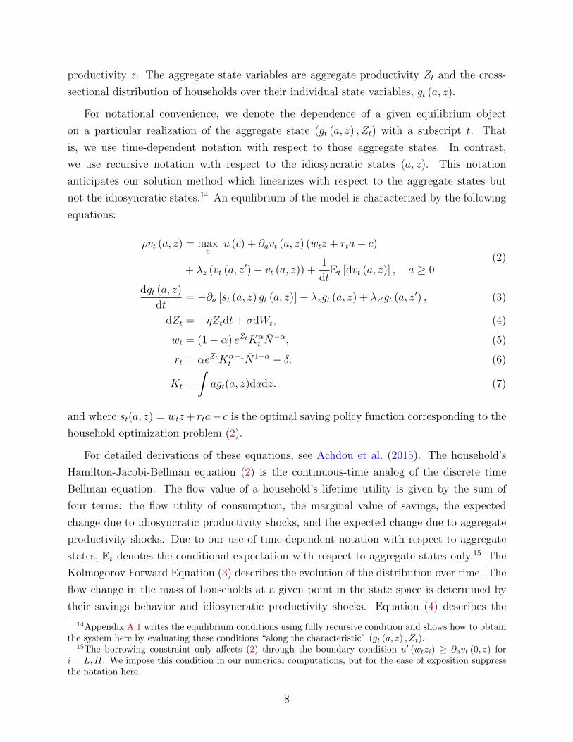
not the idiosyncratic states.14 An equilibrium of the model is characterized by the following
equations:
ρvt (a, z) = maxc
u (c) + ∂avt (a, z) (wtz + rta− c)
+ λz (vt (a, z′)− vt (a, z)) +
1
dtEt [dvt (a, z)] , a ≥ 0
(2)
dgt (a, z)
dt= −∂a [st (a, z) gt (a, z)]− λzgt (a, z) + λz′gt (a, z
′) , (3)
dZt = −ηZtdt+ σdWt, (4)
wt = (1− α) eZtKαt N
−α, (5)
rt = αeZtKα−1t N1−α − δ, (6)
Kt =
∫agt(a, z)dadz. (7)
and where st(a, z) = wtz+ rta− c is the optimal saving policy function corresponding to the
household optimization problem (2).
For detailed derivations of these equations, see Achdou et al. (2015). The household’s
Hamilton-Jacobi-Bellman equation (2) is the continuous-time analog of the discrete time
Bellman equation. The flow value of a household’s lifetime utility is given by the sum of
four terms: the flow utility of consumption, the marginal value of savings, the expected
change due to idiosyncratic productivity shocks, and the expected change due to aggregate
productivity shocks. Due to our use of time-dependent notation with respect to aggregate
states, Et denotes the conditional expectation with respect to aggregate states only.15 The
Kolmogorov Forward Equation (3) describes the evolution of the distribution over time. The
flow change in the mass of households at a given point in the state space is determined by
their savings behavior and idiosyncratic productivity shocks. Equation (4) describes the
14Appendix A.1 writes the equilibrium conditions using fully recursive condition and shows how to obtainthe system here by evaluating these conditions “along the characteristic” (gt (a, z) , Zt).
15The borrowing constraint only affects (2) through the boundary condition u′ (wtzi) ≥ ∂avt (0, z) fori = L,H. We impose this condition in our numerical computations, but for the ease of exposition suppressthe notation here.
8

evolution of aggregate productivity. Finally, equations (5) to (7) define prices given the
aggregate state.
We define a steady state as an equilibrium with constant aggregate productivity Zt = 0
and a time-invariant distribution g(a, z). The steady state system is given by
ρv (a, z) = maxc
u (c) + ∂av (a, z) (wz + ra− c) + λz (v (a, z′)− v (a, z)) , a ≥ 0 (8)
0 = −∂a [s (a, z) g (a, z)]− λzg (a, z) + λz′g (a, z′) , (9)
w = (1− α)KαN−α, (10)
r = αKα−1N1−α − δ, (11)
K =
∫ag(a, z)dadz. (12)
2.2 Linearization Procedure
Our linearization procedure consists of three steps. First, we solve for the steady state of
the model without aggregate shocks but with idiosyncratic shocks. Second, we take a first-
order Taylor expansion of the equilibrium conditions around the steady state, yielding a
linear system of stochastic differential equations. Third, we solve the linear system using
standard techniques. Conceptually, each of these steps is a straightforward extension of
standard linearization techniques to the heterogeneous agent context. However, the size of
heterogeneous agent models leads to a number of computational challenges which we address.
Step 1: Approximate Steady State Because households face idiosyncratic uncertainty,
the steady state value function varies over individual state variables v(a, z), and there is a
non-degenerate stationary distribution of households g(a, z). To numerically approximate
these functions we must represent them in a finite-dimensional way. We use a non-linear
approximation in order to retain the rich non-linearities and heterogeneity at the individual
level. In principle, any approximation method can be used in this step; we use the finite
difference methods outlined in Achdou et al. (2015) because they are fast, accurate, and
robust.
We approximate the value function and distribution over a discretized grid of asset hold-
ings a =(a1 = 0, a2, ..., aI)T. Denote the value function and distribution along this discrete
grid using the vectors v = (v (a1, zL) , ..., v (aI , zH))T and g = (g (a1, zL) , ..., g (aI , zH))
T;
both v and g are of dimension N × 1 where N = 2I is the total number of grid points in the
individual state space. We solve the steady state versions of (2) and (3) at each point on
9

this grid, approximating the partial derivatives using finite differences. Achdou et al. (2015)
show that if the finite difference approximation is chosen correctly, the discretized steady
state is the solution to the following system of matrix equations:
ρv = u (v) +A (v;p)v
0 = A (v;p)T g
p = F (g) .
(13)
The first equation is the approximated steady state HJB equation (8) for each point on the
discretized grid, expressed in our vector notation. The vector u (v) is the maximized utility
function over the grid and the matrix multiplication A (v;p)v captures the remaining terms
in (8). The second equation is the discretized version of the steady state Kolmogorov Forward
equation (9). The transition matrix A (v;p) is simply the transpose of the matrix from the
discretized HJB equation because it encodes how households move around the individual
state space. Finally, the third equation defines the prices p = (r, w)T as a function of
aggregate capital through the distribution g.16
Since v and g each have N entries, the total system has 2N + 2 equations in 2N + 2
unknowns. In simple models like this one, highly accurate solutions can be obtained with as
little as N = 200 grid points (i.e., I = 100 asset grid points together with the two income
states); however, in more complicated models, such as the two-asset model in Section 5, N
can easily grow into the tens of thousands. Exploiting the sparsity of the transition matrix
A (v;p) is necessary to even represent the steady state of such large models.
Step 2: Linearize Equilibrium Conditions The second step of our method is to com-
pute a first-order Taylor expansion of the model’s discretized equilibrium conditions around
steady state. With aggregate shocks, the discretized equilibrium is characterized by
ρvt = u (vt) +A (vt;pt)vt +1
dtEtdvt
dgt
dt= A (vt;pt)
T gt
dZt = −ηZtdt+ σdWt
pt = F (gt;Zt) .
(14)
16 The fact that prices are an explicit function of the distribution is a special feature of the Krusell andSmith (1998) model. In general, market clearing conditions take the form F(v,g,p) = 0. Our solutionmethod also handles this more general case.
10

The system (14) is a non-linear system of 2N +3 stochastic differential equations in 2N +3
variables (the 2N+2 variables from the steady state, plus aggregate productivity Zt). Shocks
to TFP Zt induce fluctuations in marginal products and therefore prices pt = F (gt;Zt).
Fluctuations in prices in turn induce fluctuations in households’ decisions and therefore in
vt and the transition matrix A (vt;pt).17 Fluctuations in the transition matrix then induce
fluctuations in the distribution of households gt.
The key insight is that this large-dimensional system of stochastic differential equations
has exactly the same structure as more standard representative agent models which are
normally solved by means of linearization methods. To make this point, Appendix A.2
relates the system (14) to the real business cycle (RBC) model. The discretized value
function points vt are jump variables, like aggregate consumption Ct in the RBC model.
The discretized distribution gt points are endogenous state variables, like aggregate capital
Kt in the RBC model. TFP Zt is an exogenous state variable. Finally, the wage and real
interest rate are statically defined variables, just as in the Krusell and Smith (1998) model.
As already anticipated, we exploit this analogy and solve the non-linear system (14)
by linearizing it around the steady state. Since the dimension of the system is large it is
impossible to compute derivatives by hand. We use a recently developed technique called
automatic (or algorithmic) differentiation that is fast and accurate up to machine precision.
It dominates finite differences in terms of accuracy and symbolic differentiation in terms of
speed. Automatic differentiation exploits the fact that the computer represents any function
as the composition of various elementary functions, such as addition, multiplication, or
exponentiation, which have known derivatives. It builds the derivative of the original function
by iteratively applying the chain rule. This allows automatic differentiation to exploit the
sparsity of the transition matrix A (vt;pt) when taking derivatives, which is essential for
numerical feasibility in large models.18
17We have written the price vector pt as a function of the state vector to easily exposit our methodologyin a way that directly extends to models with more general market clearing conditions (see footnote 16).However, this approach is not necessary in the Krusell and Smith (1998) model because we can simplysubstitute the expression for prices directly into the households’ budget constraint and hence the matrixA(vt;pt).
18To the best of our knowledge, there is no existing open-source automatic differentiation package forMatlab which exploits sparsity. We therefore wrote our own package for the computational toolbox.
11

The first-order Taylor expansion of (14) can be written as:19
Et
dvt
dgt
dZt
0
=
Bvv 0 0 Bvp
Bgv Bgg 0 Bgp
0 0 −η 0
0 Bpg BpZ −I
vt
gt
Zt
pt
dt (15)
The variables in the system, vt, gt, Zt and pt, are expressed as deviations from their steady
state values, and the matrix is composed of the derivatives of the equilibrium conditions
evaluated at steady state. Since the pricing equations are static, the fourth row of this
matrix equation only has non-zero entries on the right hand side.20 It is convenient to
plug the pricing equations pt = Bpggt +BpZZt into the remaining equations of the system,
yielding
Et
dvt
dgt
dZt
=
Bvv BvpBpg BvpBpZ
Bgv Bgg +BgpBpg BgpBpZ
0 0 −η
︸ ︷︷ ︸
B
vt
gt
Zt
dt. (16)
Step 3: Solve Linear System The final step of our method is to solve the linear system
of stochastic differential equations (16). Following standard practice, we perform a Schur
decomposition of the matrix B to identify the stable and unstable roots of the system. If
the Blanchard and Kahn (1980) condition holds, i.e., the number of stable roots equals the
19To arrive at (15), we first rearrange (14) so that all time derivatives are on the left-hand side. We thentake the expectation of the entire system and use the fact that the expectation of a Brownian increment iszero Et[dWt] = 0 to write (14) compactly without the stochastic term as
Et
dvt
dgt
dZt
0
=
u (vt;pt) +A (vt;pt)vt − ρvt
A (vt;pt)Tgt
−ηZt
F (gt;Zt)− pt
dt.
Finally, we linearize this system to arrive at (15). Note that this compact notation loses the informationcontained in the stochastic term dWt. However, since we linearize the system, this is without loss of generality– as we discuss later linearized systems feature certainty equivalence.
20The special structure of the matrix B involving zeros is particular to the Krusell and Smith (1998) modeland can be relaxed. In addition, the fact that we can express prices as a static function of gt and Zt is aspecial feature of the model; more generally, the equilibrium prices are only defined implicitly by a set ofmarket clearing conditions.
12

number of state variables gt and Zt, then we can compute the solution:
vt = Dvggt +DvZZt,
dgt
dt= (Bgg +BgpBpg +BgvDvg)gt + (BgpBpZ +BgvDvZ)Zt,
dZt = −ηZtdt+ σdWt,
pt = Bpggt +BpZZt.
(17)
The first line of (17) sets the control variables vt as functions of the state variables gt and
Zt, i.e. the matrices Dvg and DvZ characterize the optimal decision rules as a function
of aggregate states. The second line plugs that solution into the system (16) to compute
the evolution of the distribution. The third line is the stochastic process for the aggregate
productivity shock and the fourth line is the definition of prices pt.
2.3 What Does Linearization Capture and What Does It Lose?
Our method uses a mix of nonlinear approximation with respect to individual state variables
and linear approximation with respect to aggregate state variables. Concretely, from the
first line of (17), the approximated solution for the value function is of the form
vt(ai, zj) = v(ai, zj) +I∑
k=1
2∑ℓ=1
Dvg[i, j; k, l](gt(ak, zℓ)− g(ak, zℓ)) +DvZ [i, j]Zt, (18)
where Dvg[i, j; k, l] and DvZ [i, j] denote the relevant elements of Dvg and DvZ , and v(a, z)
and g(a, z) are the steady state value function and distribution. Given the value function
vt(ai, zj), optimal consumption at different points of the income and wealth distribution is
then given by
ct(ai, zj) = (∂avt(ai, zj))−1/θ. (19)
Certainty Equivalence Expressions (18) and (19) show that our solution features cer-
tainty equivalence with respect to aggregate shocks; the standard deviation σ of aggregate
TFP Zt does not enter households’ decision rules.21 This is a generic feature of all lineariza-
tion techniques.
However, our solution does not feature certainty equivalence with respect to idiosyncratic
shocks, because the distribution of idiosyncratic shocks enters the HJB equation (2) as well
21Note that σ does not enter the matrix B characterizing the linearized system (16) and therefore alsodoes not enter the matrices characterizing the optimal decision rules Dvg and DvZ .
13

as its linearized counterpart in (16) directly. A corollary of this is that our method does
capture the effect of aggregate uncertainty to the extent that aggregate shocks affect the
distribution of idiosyncratic shocks. For example, Bloom et al. (2014) and Bayer et al.
(2015) study the effect of “uncertainty shocks” that result in an increase in the dispersion
of idiosyncratic shocks and can be captured by our method.22
Our solution method may instead be less suitable for various asset-pricing applications in
which the direct effect of aggregate uncertainty on individual decision rules is key. In future
work we hope to encompass such applications by extending our first-order perturbation
method to higher orders, or by allowing the decision rules to depend non-linearly on relevant
low-dimensional aggregate state variables (but not the high-dimensional distribution). Yet
another strategy could be to assume that individuals are averse to ambiguity so that risk
premia survive linearization (Ilut and Schneider, 2014).
Distributional Dependence of Aggregates A common motivation for studying hetero-
geneous agent models is that the response of macroeconomic aggregates to aggregate shocks
may depend on the distribution of idiosyncratic states. For example, different joint distribu-
tions of income and wealth g(a, z) can result in different impulse responses of aggregates to
the same aggregate shock. Our solution method preserves such distributional dependence.
To fix ideas, consider the impulse response of aggregate consumption Ct to a productivity
shock Zt, starting from the steady-state distribution g(a, z). First consider the response of
initial aggregate consumption C0 only. We compute the impact effect of the shock on the
initial value function v0(a, z) and initial consumption c0(a, z) from (18) and (19). Integrate
this over households to get aggregate consumption
C0 =
∫c0(a, z)g(a, z)dadz ≈
I∑i=1
2∑j=1
c0(ai, zj)g(ai, zj)∆a∆z.
The impulse response of C0 depends on the initial distribution g0(a, z) because the elasticities
of individual consumption c0(a, z) with respect to the aggregate shock Z0 are different for
individuals with different levels of income and/or wealth. These individual elasticities are
then aggregated according to the initial distribution. Therefore, the effect of the shock
depends on the initial distribution g0(a, z).
To see this even more clearly, it is useful to briefly work with the continuous rather than
22McKay (2017) studies how time-varying idiosyncratic uncertainty on aggregate consumption dynamics.Terry (2017) studies how well discrete-time relatives of our method capture time-variation in the dispersionof productivity shocks in a heterogeneous firm model.
14

discretized value and consumption policy functions. Analogous to (18), we can write the
initial value function response as v0(a, z) = DvZ(a, z)Z0 where DvZ(a, z) are the elements
of DvZ in (17) and where we have used the fact that the initial distribution does not move
(i.e. g0(a, z) = 0) by virtue of g being a state variable. We can use this to show that
the deviation of initial consumption from steady state satisfies c0(a, z) = DcZ(a, z)Z0 where
DcZ(a, z) captures the responsiveness of consumption to the aggregate shock.23 The impulse
response of initial aggregate consumption is then
C0 =
∫DcZ(a, z)g(a, z)dadz × Z0. (20)
It depends on the steady-state distribution g(a, z) since the responsiveness of individual
consumption to the aggregate shock DcZ(a, z) differs across (a, z).
Size- and Sign-Dependence Another question of interest is whether our economy fea-
tures size- or sign-dependence, that is, whether it responds non-linearly to aggregate shocks
of different sizes or asymmetrically to positive and negative shocks.24 In contrast to state
dependence, our linearization method eliminates any potential sign- and size-dependence.
This can again be seen clearly from the impulse response of initial aggregate consumption
in (20) which is linear in the aggregate shock Z0. This immediately rules out size- and
sign-dependence in the response of aggregate consumption to the aggregate shock.25
In future work we hope to make progress on relaxing this feature of our solution method.
Extending our first-order perturbation method to higher orders would again help in this
regard. Another idea is to leverage the linear model solution together with parts of the
full non-linear model to simulate the model in a way that preserves these nonlinearities. In
particular one could use the fully nonlinear Kolmogorov Forward equation in (14) instead
of the linearized version in (16) to solve for the path of the distribution for times t > 0:
dgt/dt = A (vt;pt)T gt. This procedure allows us to preserve size-dependence after the initial
impact t > 0 because larger shocks potentially induce non-proportional movements in the
individual state space, and therefore different distributional dynamics going forward.26
23In particular DcZ(a, z) = (∂av(a, z))− 1
θ−1∂aDvZ(a, z). To see this note that c0(a, z) =
(∂av(a, z))− 1
θ−1∂av0(a, z) = (∂av(a, z))− 1
θ−1∂aDvZ(a, z)Z0 := DcZ(a, z)Z0.24Note that this is separate from the state dependence we just discussed which is concerned with how the
distribution may affect the linear dynamics of the system.25Note that expression (20) only holds at t = 0. At times t > 0, the distribution also moves gt(a, z) = 0.
The generalization of (20) to t > 0 is Ct ≈∫ct(a, z)g(a, z)dadz +
∫c(a, z)gt(a, z)dadz. Since both ct(a, z)
and gt(a, z) will be linear in Zt, so will be Ct, again ruling out size- and sign-dependence.26An open question is under what conditions this procedure would be consistent with our use of linear
approximations to solve the model. One possible scenario is as follows: even though the time path for the
15

Small versus Large Aggregate Shocks Another generic feature of linearization tech-
niques is that the linearized solution is expected to be a good approximation to the true
non-linear solution for small aggregate shocks and less so for large ones. Section 2.4 below
documents that our approximate dynamics of the distribution is accurate for the typical
calibration of TFP shocks in the Krusell and Smith (1998) model, but breaks down for very
large shocks.27
2.4 Performance of Linearization in Krusell-Smith Model
In order to compare the performance of our method to previous work, we solve the model
under the parameterization of the JEDC comparison project Den Haan, Judd and Julliard
(2010). A unit of time is one quarter. We set the rate of time preference ρ = 0.01 and the
coefficient of relative risk aversion θ = 1. Capital depreciates at rate δ = 0.025 per quarter
and the capital share is α = 0.36. We set the levels of idiosyncratic labor productivity zL
and zH following Den Haan, Judd and Julliard (2010).
One difference between our model and Den Haan, Judd and Julliard (2010) is that
we assume aggregate productivity follows the continuous-time, continuous-state Ornstein-
Uhlenbeck process (1) rather than the discrete-time, two-state Markov chain in Den Haan,
Judd and Julliard (2010). To remain as consistent with Den Haan, Judd and Julliard (2010)’s
calibration as possible, we choose the approximate quarterly persistence corr(logZt+1, logZt) =
e−η ≈ 1− η = 0.75 and the volatility of innovations σ = 0.007 to match the standard devia-
tion and autocorrelation of Den Haan, Judd and Julliard (2010)’s two-state process.28
In our approximation we set the size of the individual asset grid I = 100, ranging from
a1 = 0 to aI = 100. Together with the two values for idiosyncratic productivity, the total
number of grids is N = 200 and the total size of the dynamic system (16) is 400.29
Table 1 shows that our linearization method solves the Krusell and Smith (1998) model
in approximately one quarter of one second. In contrast, the fastest algorithm documented
distribution might differ substantially when computed using the non-linear Kolmogorov Forward equation,the time path for prices may still be well approximated by the linearized solution. Hence, the error in theHJB equation from using the linearized prices may be small.
27Related, our linearization method obviously rules out nonlinear amplification effects that result in abimodal ergodic distribution of aggregate states as in He and Krishnamurthy (2013) and Brunnermeier andSannikov (2014).
28Another difference is that Den Haan, Judd and Julliard (2010) allows the process for idiosyncratic shocksto depend on the aggregate state. We set our idiosyncratic shock process to match the average transitionprobabilities in Den Haan, Judd and Julliard (2010).
29In this calculation, we have dropped one grid point from the distribution using the restriction that thedistribution integrates to one. Hence there are N = 200 equations for vt, N − 1 = 199 equations for gt andone equation for Zt.
16

Table 1: Run Time for Solving Krusell-Smith Model
Full Model
Steady State 0.082 sec
Derivatives 0.021 sec
Linear system 0.14 sec
Simulate IRF 0.024 sec
Total 0.27 sec
Notes: Time to solve Krusell-Smith model once on MacBook Pro 2016 laptop with 3.3 GHz processor and16 GB RAM, using Matlab R2016b and our code toolbox. “Steady state” reports time to compute steadystate. “Derivatives” reports time to compute derivatives of discretized equilibrium conditions. “Linearsystem” reports time to solve system of linear differential equations. “Simulate IRF” reports time tosimulate impulse responses reported in Figure 1. “Total” is the sum of all these tasks.
in the comparison projection by Den Haan (2010) takes over seven minutes to solve the
model – more than 1500 times slower than our method (see Table 2 in Den Haan (2010)).30
In Section 3 we solve the model in approximately 0.1 seconds using our model-free reduction
method.
Accuracy of Linearization The key restriction that our method imposes is linearity
with respect to the aggregate state variables Zt and gt. We evaluate the accuracy of this
approximation using the error metric suggested by Den Haan (2010). The Den Haan error
metric compares the dynamics of the aggregate capital stock under two simulations of the
model for T = 10, 000 periods. The first simulation computes the path of aggregate capital
Kt from our linearized solution (17). The second simulation computes the path of aggregate
capital K∗t from simulating the model using the nonlinear dynamics (3) as discussed in
Section 2.3. We then compare the maximum log difference between the two series,
ϵDH = 100× maxt∈[0,T ]
|logKt − logK∗t | .
Den Haan originally proposed this metric to compute the accuracy of the forecasting rule
in the Krusell and Smith (1998) algorithm; in our method, the linearized dynamics of the
distribution gt are analogous to the forecasting rule.
30As discussed by Den Haan (2010), there is one algorithm (Penal) that “is even faster, but this algorithmdoes not solve the actual [Krusell-Smith] model specified.”
17

Table 2: Maximum den Haan Error in %
St. Dev Productivity Shocks (%) Maximum den Haan Error (%)
0.01 0.000
0.1 0.001
0.7 0.049
1.0 0.118
5.0 3.282
Notes: Maximum percentage error in accuracy check suggested by Den Haan (2010). The error is thepercentage difference between the time series of aggregate capital under our linearized solution and anonlinear simulation of the model, as described in the main text. The bold face row denotes the calibratedvalue σ = 0.007.
When the standard deviation of productivity shocks is 0.7%, our method gives a max-
imum percentage error ϵDH = 0.049%, implying that households in our model make small
errors in forecasting the distribution. Our method is three times as accurate as the Krusell
and Smith (1998) method, which is the most accurate algorithm in Den Haan (2010) and
gives ϵDH = 0.16%. Table 2 shows that, since our method is locally accurate, its accuracy
decreases in the size of the shocks σ. However, with the size of aggregate shocks in the
baseline calibration, it provides exceptional accuracy.
3 Model Reduction
Solving the linear system (16) is extremely efficient because the Krusell and Smith (1998)
model is relatively small. However, the required matrix decomposition becomes prohibitively
expensive in larger models like the two-asset model that we will study in Section 5. We must
therefore reduce the size of the system to solve these more general models. Furthermore,
even in smaller models like Krusell and Smith (1998), model reduction makes likelihood-
based estimation feasible by reducing the size of the associated filtering problem.31
In this section, we develop a model-free reduction method to reduce the size of the
linear system while preserving accuracy. Our approach projects the high-dimensional dis-
31Mongey and Williams (2016) use a discrete-time relative of our method without model reduction toestimate a small heterogeneous firm model. Winberry (2016) provides an alternative parametric approachfor reducing the distribution and also uses it to estimate a small heterogeneous firm model.
18

tribution gt and value function vt onto low-dimensional subspaces and solves the resulting
low-dimensional system. The main challenge is reducing the distribution, which we discuss
in Sections 3.1, 3.2, and 3.3. Section 3.4 describes how we reduce the value function. Section
3.5 puts the two together to solve the reduced model and describes the numerical implemen-
tation. Finally, Section 3.6 shows that our reduction method performs well in the Krusell
and Smith (1998) model.
In order to simplify notation, for the remainder of this section we use vt,gt and pt to
denote the deviations from steady state in the value function, distribution, and prices. In
Section 2, we had denoted these objects using vt, gt and pt. This change of notation applies
to Section 3 only, and we will remind the reader whenever this change could cause confusion.
3.1 Overview of Distribution Reduction
The basic insight that we exploit is that only a small subset of the information in gt is
necessary to accurately forecast the path of prices pt. In fact, in the discrete time version of
this model, Krusell and Smith (1998) show that just the mean of the asset distribution gt
is sufficient to forecast pt according to a forecast-error metric. However, the success of their
reduction strategy relies on the economic properties of the model, so it is not obvious how
to generalize it to other environments. We use a set of tools from the engineering literature
known as model reduction to generalize Krusell and Smith (1998)’s insight in a model-free
way, allowing the computer to compute the features of the distribution that are necessary
to accurately forecast pt.32
It is important to note that the vector pt does not need to literally consist of prices; it
is simply the vector of objects we wish to accurately describe. In practice, we often also
include other variables of interest, such as aggregate consumption or output, to ensure that
the reduced model accurately describes their dynamics as well.
32The following material is based on lecture notes by Amsallem and Farhat (2011), which in turn buildon a book by Antoulas (2005). Lectures 3 and 7 by Amsallem and Farhat (2011) and Chapters 1 and 11 inAntoulas (2005) are particularly relevant. All lecture notes for Amsallem and Farhat (2011) are availableonline at https://web.stanford.edu/group/frg/course_work/CME345/ and the book by Antoulas (2005)is available for free at http://epubs.siam.org/doi/book/10.1137/1.9780898718713. Also see Reiter(2010) who applies related ideas from the model reduction literature in order to reduce the dimensionalityof a linearized discrete-time heterogeneous agent model.
19

3.1.1 The Distribution Reduction Problem
We say that the distribution exactly reduces if there exists a kS-dimensional time-invariant
subspace S with kS << N such that, for all distributions gt which occur in equilibrium,
gt = γ1tx1 + γ2tx2 + ...+ γkS txkS ,
where XS = [x1, ...,xkS ] ∈ RN×kS is a basis for the subspace S and γ1t, ..., γkS t are scalars. If
we knew the time-invariant basis XS , we could decrease the dimensionality of the problem
by tracking only the kS−dimensional vector of coefficients γt.
Typically exact reduction as described above does not hold, so we instead must estimate
a trial basis X = [x1, ...,xk] ∈ RN×k such that the distribution approximately reduces, i.e.,
gt ≈ γ1tx1 + γ2tx2 + ...+ γktxk,
or, in matrix form, gt ≈ Xγt. Denote the resulting approximation of the distribution by
gt = Xγt and the approximate prices by pt = Bpggt +BpZZt.
Our model maps directly into the prototypical problem considered by the model reduction
literature if the decision rules are exogenous, i.e. the matrices Dvg and DvZ in (17) are
exogenously given.33 This case assumes away a crucial part of the economics we are interested
in studying but nevertheless has pedagogical use in connecting to the existing literature. In
this case, using the second and fourth equations of (17) and recalling our convention in this
section to drop hats from variables, our dynamical system becomes
dgt
dt= Cgggt +CgZZt
pt = Bpggt +BpZZt,(21)
where Cgg = Bgg + BgpBpg + BgvDvg and CgZ = BgpBpZ + BgvDvZ . This system maps
a low-dimensional vector of “inputs” (aggregate productivity Zt) into a low-dimensional
vector of “outputs” (prices pt), intermediated through the high-dimensional distribution
gt.34 The model reduction literature provides an off-the-shelf set of tools to replace the high-
33Exogenous decision rules usually relate the value function to prices, i.e. vt = Dvppt. But pricespt = Bpggt +BpZZt in turn depend on the distribution gt and productivity Zt. Hence so do the decisionrules: vt = Dvggt +DvZZt, with Dvg = DvpBpg and DvZ = DvpDpZ .
34The system (21) is called a linear time invariant (LTI) system. Zt is an input into the system and pt
is an output. If both inputs and outputs are scalars, the system is called a single-input-single-output (SISO)system. If both inputs and outputs are vectors, it is called a multiple-input-multiple-output (MIMO) system.Instead of assuming that decision rules are exogenous, we could have assumed that there is no feedback
20

dimensional “intermediating variable” gt with a low-dimensional approximation γt while
preserving the mapping from inputs to outputs.
Of course, our economic model is more complicated than this special case because the
distribution reduction feeds back into agents’ decisions through the endogenous value func-
tion vt. It is helpful to restate the system with endogenous vt in a form closer to that in the
model reduction literature:[Et[dvt]
dgt
]=
[Bvv BvpBpg
Bgv Bgg +BgpBpg
][vt
gt
]dt+
[BvpBpZ
BgpBpZ
]Ztdt
pt = Bpggt +BpZZt,
(22)
given the exogenous stochastic process for productivity (4). This system still maps the
low-dimensional input Zt into the low-dimensional output pt. However, the intermediating
variables are now both the distribution gt and the forward-looking decisions vt.
3.1.2 Deriving The Reduced System Given Basis X
Model reduction involves two related tasks: first, given a trial basis X, we must compute the
dynamics of the reduced system in terms of the distribution coefficients γt; and second, we
must choose the basis X itself. In this subsection, we complete the first step of characterizing
the reduced system given a basis X, which is substantially easier than the second step of
choosing the basis. Sections 3.2 and 3.3 discuss how we choose the basis.
Mathematically, we project the distribution gt onto the subspace spanned by the basis
X ∈ RN×k. Write the requirement that gt ≈ Xγt as
gt = Xγt + εt, (23)
where εt ∈ RN is a residual. The formulation (23) is a standard linear regression in which the
distribution gt is the dependent variable, the basis vectors X are the independent variables,
and the coefficients γt are to be estimated.
Just as in ordinary least squares, we can estimate the projection coefficients γt by im-
posing the orthogonality condition XTεt = 0, giving the familiar formula
γt = (XTX)−1XTgt. (24)
from individuals’ decisions to the distribution Bgv = 0. In that case the system (16) again becomes abackward-looking system of the LTI form (21), now with Cgg = Bgg +BgpBpg and CgZ = BgpBpZ .
21

A sensible basis will be orthonormal, so that (XTX)−1 = I, further simplifying (24) to
γt = XTgt.35 We can compute the evolution of this coefficient vector by differentiating (24)
with respect to time and using (23) to get
dγtdt
= XTdgtdt
= XTBgvvt +XT (Bgg +BgpBpg) (Xγt + εt) +XTBgpBpgZt
≈ XTBgvvt +XT (Bgg +BgpBpg)Xγt +XTBgpBpgZt.
The hope is that the residuals εt are small and so the last approximation is good. Assuming
this is the case, we have the reduced version of (22)[Et[dvt]
dγt
]=
[Bvv BvpBpgX
XTBgv XT (Bgg +BgpBpg)X
][vt
γt
]dt+
[BvpBpZ
XTBgpBpZ
]Ztdt,
pt = BpgXγt +BpZZt.
(25)
Summing up, assuming we have the basis X, this projection procedure takes us from the
system of differential equations involving the N -dimensional vector gt in (22) to a system
involving only the k-dimensional vector γt in (25).36
3.2 Choosing the Basis X with Exogenous Decision Rules
We now turn to choosing a good basis X. In this section we explain how to choose a basis in
a model with exogenous decision rules, allowing us to use preexisting tools from the model
reduction literature. In Section 3.3 we extend the strategy to the case with endogenous
decision rules.
Mechanically increasing the size of the basis X will improve the approximation of the
distribution gt; in the limit whereX spans RN , we will not reduce the distribution at all. The
goal of the model reduction literature is to provide a good approximation of the mapping
from inputs Zt to outputs pt with as small a basis X as possible. We operationalize the
notion of a “good approximation” by matching the impulse response function of pt to a
35The assumption that X is orthonormal is not necessary to derive our results but makes the expositiontransparent. Appendix A.3 derives our results using non-normalized projection matrices.
36The model reduction literature also presents alternatives to our “least squares” approach to computingthe coefficients γt. In particular, one can also estimate γt using what amounts to an instrumental variablesstrategy: one can define a second subspace spanned by the columns of some matrix Z and impose theorthogonality condition ZTεt = 0. This yields an alternative estimate γt = (ZTX)−1ZTgt. Mathematically,this is called an oblique projection (as opposed to an orthogonal projection) of gt onto the k-dimensionalsubspace spanned by the columns X along the kernel of ZT. See Amsallem and Farhat (2011, Lecture 3)and Antoulas (2005) for more detail on oblique projections.
22
shock to Zt up to a specified order k.37
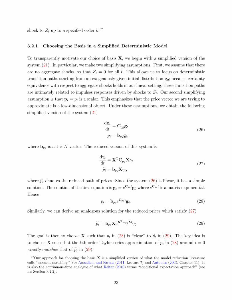
3.2.1 Choosing the Basis in a Simplified Deterministic Model
To transparently motivate our choice of basis X, we begin with a simplified version of the
system (21). In particular, we make two simplifying assumptions. First, we assume that there
are no aggregate shocks, so that Zt = 0 for all t. This allows us to focus on deterministic
transition paths starting from an exogenously given initial distribution g0; because certainty
equivalence with respect to aggregate shocks holds in our linear setting, these transition paths
are intimately related to impulses responses driven by shocks to Zt. Our second simplifying
assumption is that pt = pt is a scalar. This emphasizes that the price vector we are trying to
approximate is a low-dimensional object. Under these assumptions, we obtain the following
simplified version of the system (21)
dgt
dt= Cgggt
pt = bpggt,(26)
where bpg is a 1×N vector. The reduced version of this system is
dγtdt
= XTCggXγt
pt = bpgXγt,(27)
where pt denotes the reduced path of prices. Since the system (26) is linear, it has a simple
solution. The solution of the first equation is gt = eCggtg0 where eCggt is a matrix exponential.
Hence
pt = bpgeCggtg0. (28)
Similarly, we can derive an analogous solution for the reduced prices which satisfy (27)
pt = bpgXeXTCggXtγ0 (29)
The goal is then to choose X such that pt in (28) is “close” to pt in (29). The key idea is
to choose X such that the kth-order Taylor series approximation of pt in (28) around t = 0
exactly matches that of pt in (29).
37Our approach for choosing the basis X is a simplified version of what the model reduction literaturecalls “moment matching.” See Amsallem and Farhat (2011, Lecture 7) and Antoulas (2005, Chapter 11). Itis also the continuous-time analogue of what Reiter (2010) terms “conditional expectation approach” (seehis Section 3.2.2).
23

The Taylor-series approximation of the time path of prices (28) around t = 0 is38
pt ≈ bpg
[I+Cggt+
1
2C2
ggt2 + . . .+ 1
(k−1)!Ck−1
gg tk−1
]g0 (30)
where we have used that eCggt ≈ I+Cggt+12C2
ggt2 + .... Similarly, the Taylor-series approx-
imation of reduced prices is
pt ≈ bpgX
[I+ (XTCggX)t+
1
2(XTCggX)2t+ . . .+ 1
(k−1)!(XTCggX)k−1tk−1
]γ0. (31)
We want to chooseX so that the first k terms of the two Taylor series expansions are identical.
With γ0 = XTg0, this means that we require bpg = bpgXXT, bpgCgg = bpgXXTCggXXT,
and so on. If γt has the same dimensionality as gt (k = N , i.e., we are not reducing the
distribution at all), then X has to be orthogonal, i.e. XXT = I, and the conclusion trivially
follows. But once we have proper reduction, this equality does not hold, and the problem
of Taylor series coefficient matching becomes non-trivial. Fortunately, the model reduction
literature gives us a systematic way for choosing X such that (30) matches (31). This
systematic way builds upon what is known as the order-k observability matrix of the system
(26):39
O(bpg,Cgg) :=
bpg
bpgCgg
bpgC2gg
...
bpgCk−1gg
. (32)
It turns out that if the basis X spans the subspace generated by the transpose of the observ-
ability matrix O(bpg,Cgg), then the kth-order Taylor-series approximation of reduced prices
(31) exactly matches that of unreduced prices (30), even though it only uses information
on the reduced state vector γt. Showing this just requires a few lines of algebra, which we
present in Appendix A.3.1.
38In this simple deterministic model, (30) can also be derived in a simpler fashion: the Taylor-series
approximation around t = 0 is pt ≈ p0 + p0t +12 p0t
2 + ... + 1(k−1)!p
(k−1)0 tk−1. This is equivalent to (30)
because the derivatives are given by pt = bpggt = bpgCgggt, pt = bpgC2gggt and so on. This strategy no
longer works in the full model with aggregate productivity shocks. In contrast, the derivation in terms ofthe matrix exponential eCggt can be easily extended to the stochastic case.
39Observability of a dynamical system is an important concept in control theory introduced by RudolfKalman, the inventor of the Kalman filter. It is a measure of how well a system’s states (here gt) can beinferred from knowledge of its outputs (here pt). For systems like ours observability can be directly inferredfrom the observability matrix O(bpg,Cgg) with k = N . Note that some texts refer only to O(bpg,Cgg) withk = N as “observability matrix” and to the matrix with k < N as “partial observability matrix.”
24
To gain some intuition why the observability matrix (32) makes an appearance, note that
the Taylor-series approximation (30) can be written more compactly using matrix notation
as
pt ≈[1, t, 1
2t2, ..., 1
(k−1)!tk−1
]O(bpg,Cgg)g0
Related, O(bpg,Cgg)gt is simply the vector of time derivatives of pt, i.e. pt, pt and so on (see
footnote 38).
3.2.2 Choosing the Basis in The Stochastic Model
The deterministic case makes clear that the observability matrix O(bpg,Cgg) plays a key
role in model reduction. The logic of this simple case carries through the stochastic model,
but the full derivation is more involved and details can be found in Appendix A.3. Because
the model is now stochastic, the correct notion of “matching the path of prices” is to match
the impulse response function of prices.
Proposition 1. Consider the stochastic model with exogenous decision rules (21). Let X
be a basis which spans the subspace generated by the observability matrix O(bpg,Cgg)T with
Cgg = Bgg+Bgpbpg+BgvDvg. Then the impulse response function of prices pt to an aggregate
productivity shock Zt in the reduced model equals the impulse response function of prices pt
in the unreduced model up to order k.
Proof. See Appendix A.3.2
The impulse response function in the stochastic model combines the impact effect of an
aggregate shock Zt together with the transition back to steady state. We do not reduce
the exogenous state variable Zt, so the reduced model captures the impact effect of a shock
exactly. The role of the observability matrix is to approximate the transition back to steady
state analogously to the deterministic case.
Finally, note that in this section we have assumed pt is a scalar to emphasize that it is
a low-dimensional object. In general pt is an ℓ × 1 vector. One can extend the argument
above to show that the correct basis X spans the subspace generated by O(Bpg,Cgg)T for
Cgg = Bgg+BgpBpg+BgvDvg where now Bpg is an ℓ×N matrix. Matching impulse response
functions of pt up to order k, requires matching ℓk terms in the corresponding Taylor-series
approximation and hence the observability matrix O(Bpg,Cgg) is now of dimension kg ×N ,
where kg = ℓk < N .
25

3.3 Choosing the Basis X with Endogenous Decision Rules
Section 3.2 shows that if decision rules Dvg are exogenously given, then choosing the basis X
to span the subspace generated by O(Bpg,Cgg)T guarantees that the impulse response of the
reduced price pt matches the unreduced model up to a pre-specified order k. However, when
decision rules are endogenous, the choice of basis impacts agents’ decisions and therefore the
evolution of the distribution. In this case, the results of Section 3.2 do not apply.
However, the choice of basis in Section 3.2 was only dictated by the concern of efficiently
approximating the distribution with as small a basis as possible; it is always possible to
improve accuracy by adding additional orthogonal basis vectors. In fact, in the finite limit
when k = N , any linearly independent basis spans all of RN so the distribution is not
reduced at all and the reduced model is vacuously accurate. Therefore, setting the basis X
to the subspace generated by O(Bpg,Bgg+BgpBpg)T, i.e. ignoring feedback from individuals’
decisions to the distribution by effectively setting Dvg = 0, will not be efficient but may still
be accurate. In practice, we have found in both the simple Krusell and Smith (1998) model
and the two-asset model in Section 5 that this choice leads to accurate solutions for high
enough order k of the observability matrix.
In cases where choosing the basis to span the subspace O(Bpg,Bgg + BgpBpg)T is not
accurate even for as high an order k as numerically feasible, we suggest an iterative procedure.
First, we solve the reduced model (25) based on the inaccurate basis choice for the subspace
O(Bpg,Bgg +BgpBpg)T. This yields decision rules Dvγ defining a mapping from the reduced
distribution γt to the value function. We then use these to construct an approximation
to the true decision rules Dvg (which map the full distribution to the value function), i.e.
Dvg = DvγXT.40 Next we choose a new basis of the subspace generated by O(Bpg,Bgg +
Bgg + BgpBpg + BgvDvg)T and solve the model again based on the new reduction. If the
second reduction gives an accurate solution, we are done; if not, we continue the iteration.
Although we have no theoretical guarantee that this iteration will converge, in practice we
have found that it does.
Choosing k and Internal Consistency with Endogenous Decision Rules A key
practical step in reducing the distribution is choosing the order of the observability matrix
k, which determines the size of the basis X. With exogenous decision rules, we showed that
a basis of order k implies that the path of reduced prices pt matches the k-th order Taylor
40Recall from (24) that the projection of gt onto X defines the reduced distribution as γt = XTgt. Hence
the optimal decision rule can be written as vt = Dvγγt = DvγXTgt = Dvggt where Dvg = DvγX
T.
26

expansion of the path of true prices pt, providing a natural metric for assessing accuracy.41
However, this logic does not carry through with endogenous decision rules, leaving unclear
what exactly a basis of order k captures.
In the finite limit when k = N , any linearly independent basis spans all of RN so the
distribution is not reduced at all and the reduced model is vacuously accurate. Hence,
a natural procedure is to increase k until the dynamics of reduced prices converge. In
practice, this convergence is often monotonic. However, we cannot prove convergence is
always monotonic, still leaving open the question of what exactly the reduced model captures
for a given order k.
We suggest an internal consistency metric to assess the extent to which the reduced
model satisfies the model’s equilibrium conditions. The spirit of our internal consistency
check is similar to Krusell and Smith (1998)’s R2 forecast-error metric and Den Haan (2010)’s
accuracy measure discussed in Section 2: if agents make decisions based on the price path
implied by the reduced distribution, but we aggregate those decisions against the true full
distribution, do the prices generated by the true distribution match the forecasts?
Concretely, our internal consistency check consists of three steps. First, we compute
households’ decisions based on the reduced distribution, vt = Dvγγt. Second, we use these
decisions to simulate the nonlinear dynamics of the full distribution g∗t – not the reduced
version γt – and its implied prices p∗t for a given path of aggregate shocks Zt
p∗t = Bpgg
∗t +BpZZt
dg∗t
dt= A(vt,p
∗t )g
∗t ,
where A(vt, p∗t ) is the nonlinear transition matrix implied by the decision rules vt and price
p∗t . The third step of our internal accuracy check is to assess the extent to which the dynamics
of p∗t matches the dynamics implied by the reduced system pt. If the two paths are close,
households in the reduced model could not significantly improve their forecasts by using
additional information about the distribution. Once again, we compare the maximum log
deviation of the two paths
ϵ = maxi
maxt≥0
|log pit − log p∗it| ,
where i denotes an entry in the price vector.
41Recall that in general pt includes both prices and other observables of interest to the researcher.
27

Computing The Basis X Following the discussion above, we choose the basis X to span
the subspace generated by O(Bpg,Bgg +BgpBpg)T. However, using O(Bpg,Bgg +BgpBpg)
T
directly is numerically unstable due to approximate multicollinearity; as in standard regres-
sion, high degree standard polynomials are nearly collinear due to the fact that, for large
k, Bpg(Bgg + BgpBpg)k−2 ≈ Bpg(Bgg + BgpBpg)
k−1, leaving the necessary projection of the
distribution onto X numerically intractable.
We overcome this challenge by relying on a Krylov subspace method, an equivalent but
more numerically stable class of methods.42 For any N ×N matrix A and N × 1 vector b,
the order-k Krylov subspace is
Kk(A,b) = span({
b,Ab,A2b, ...,Ak−1b})
.
From this definition it can be seen that the subspace spanned by the columns of O(Bpg,Bgg+
BgpBpg)T is simply the order-k Krylov subspace generated by (Bgg + BgpBpg)
T and BTpg,
i.e. Kk(BTgg + BT
gpBTpg,B
Tpg). Therefore, the projection of gt on O(Bpg,Bgg + BgpBpg)
T is
equivalent to the projection of gt onto this Krylov subspace.
There are many methods for projecting onto Krylov subspaces in the literature. One
important feature of all these methods is that they take advantage of the sparsity of the
underlying matrices.43 We have found that one particular method, deflated block Arnoldi
iteration, is a robust procedure. Deflated block Arnoldi iteration has two advantages for
our application. First, it is a stable procedure to orthogonalize the columns of the basis X
and eliminate the approximate multicollinearity. Second, the deflation component handles
multicollinearity that can arise even with non-deflated block Arnoldi iteration.
3.4 Value Function Reduction
After reducing the dimensionality of the distribution gt, we are left with a system of di-
mension N + kg with kg << N (recall kg = ℓ × k where ℓ is the number of prices and k is
the order of the approximation according to which the basis X is chosen). Although this is
considerably smaller than the original system which was of size 2N , it is still large because
it contains N equations for the value function – one for each point in the individual state
42See Antoulas (2005, Chapter 11) and Amsallem and Farhat (2011, Lecture 7).43Even though Bgg is sparse and Bgp and Bpg are only ℓ×N , the matrix Bgg +BgpBpg which actually
enters the system (22) is N × N and not sparse (because BgpBpg is N × N not sparse). In the two-assetmodel in Section 5, N = 66, 000, and even storing this matrix is not feasible. Fortunately it is never actuallynecessary to compute this full matrix; instead, it is only necessary to compute Bpg(Bgg + BgpBpg) whichinvolves the action of BgpBpg on a thin ℓ×N matrix Bpg and can be computed as (BpgBgp)Bpg.
28

space. In complex models, this leaves the linear system too large for matrix decomposition
methods to be feasible.44
We therefore also reduce the dimensionality of the distribution vt. Just like in our
method for reducing the distribution gt, we project the (deviation from steady state of the)
value function vt onto a lower-dimensional subspace. As before, an important question
is how to choose the basis for this projection. We choose it by appealing to the theory
for approximating smooth functions and approximate vt using splines. In most models,
the value function is sufficiently smooth that a low-dimensional spline provides an accurate
approximation. In particular, any spline approximation can be written as the projection
vt ≈ Xvνt,
where Xv is a N × kv matrix defining the spline knot points and νt are the kv coeffi-
cients at those knot points.45 Given this linear projection the coefficients are given by
νt = (XTvXv)
−1XTv vt = XT
v vt, where we have used that we typically choose an orthonormal
Xv so that XTvXv = I.
It is worth emphasizing the symmetry with our distribution reduction method, the pro-
jection (23). In order to do so we add a g-subscript to the basis in the distribution reduction
for the remainder of the paper and write (23) as gt ≈ Xgγt. Hence from now on Xg denotes
the basis in the reduction of the distribution gt and Xv denotes the basis in the reduction of
the value function vt. It is also important to note that we are approximating the deviation
of the value function from its steady state value, not the value function itself (the reader
should recall our convention in the present section to drop hat subscripts from variables that
are in deviation from steady state for notational simplicity).
We have found that non-uniformly spaced quadratic splines work well for three reasons.
First, the non-uniform spacing can be used to place more knots in regions of the state space
with high curvature, allowing for an efficient dimensionality reduction. Second, the quadratic
spline preserves monotonicity and concavity between knot points, which is important in com-
puting first-order conditions. Third, and related, the local nature of splines implies that they
avoid creating spurious oscillations at the edges of the state space (Runge’s phenomenon)
which often occurs with global approximations like high-degree polynomials.
44One way to overcome this challenge is to use sparse matrix methods to find just the k eigenvaluesassociated with the stable eigenvectors. This is much faster than computing the full matrix decompositionnecessary to obtain the full set of eigenvectors. However, it is slower than the approach we pursue in thissubsection.
45Note that, in general, the number of coefficients is different from the number of knot points.
29

It is also important to note the difference between approximating the deviations of the
value function from steady state using quadratic splines – which we do – versus solving for
the steady state value using quadratic splines – which we do not do. The finite difference
method we use to compute the steady state does not impose that the value function is
everywhere differentiable, which is potentially important for capturing the effects of non-
convexities. However, after having computed the steady state value functions, it is typically
the case that they have kinks at a finite number of points and are well-approximated by
smooth functions between these points. It is then straightforward to fit quadratic splines
between the points of non-differentiability.
3.5 Putting It All Together: A Numerical Toolbox
Summarizing the previous sections, we have projected the distribution gt onto the subspace
spanned by Xg and the value function vt onto the subspace spanned by Xv. Now we simply
need to keep track of the kv × 1 coefficient vector νt for the value function and the kg × 1
coefficient vector γt for the distribution. Because knowledge of these coefficients is sufficient
to reconstruct the full value function and distribution, we will also sometimes refer to νt as
the reduced value function and to γt as the reduced distribution. Our original system (16)
is now reduced to
Et
dνt
dγt
dZt
=
XTvBvvXv XT
vBvpBpgXg XTv BvpBpZ
XTg BgvXv XT
g (Bgg +BgpBpg)Xg XTg BgpBpZ
0 0 −η
νt
γt
Zt
dt. (33)
We have provided a numerical toolbox implementing the key steps in our computational
method at the github page associated with this project.46 Broadly, the user provides two
files: one which solves for the steady state and another which evaluates the model’s equilib-
rium conditions. Our toolbox then implements the following algorithm (we here revert back
to denoting deviations from steady state with hat superscripts):
1. Compute the steady state values of v,g and p.
2. Compute a first-order Taylor expansion of the equilibrium conditions (14) around
steady state using automatic differentiation, yielding the system (16) in terms of devi-
ations from steady state vt, gt, pt and Zt.
46Currently at: https://github.com/gregkaplan/phact.
30

3. If necessary, reduce the model, yielding the system (33) in terms of (νt, γt, Zt).
(a) Distribution reduction: compute the basis Xg = O(Bpg,Bgg + BgpBpg)T using
deflated Arnoldi iteration and project gt on Xg to obtain the reduced distribution
γt.
(b) Value function reduction: compute the spline basis Xv and project vt on Xv to
obtain the reduced value function νt.
4. Solve the system (16) or, if reduced, (33).
5. Simulate the system to compute impulse responses and time-series statistics.
3.6 Model Reduction in Krusell-Smith Model
The Krusell and Smith (1998) is a useful environment for evaluating our model reduction
methodology because it is possible to solve the full unreduced model as a benchmark. We
are able to substantially reduce the size of the system: projecting the distribution on an
observability matrix of order k = 1 and approximating the value function at 24 spline knot
points provides an extremely accurate approximation of the model’s dynamics.47 Figure
1 shows that the impulse responses of key aggregate variables in the reduced model are
almost exactly identical to the full, unreduced model, despite approximating the N = 400
dimensional dynamic system with a 30-dimensional system.48
The fact that we can reduce the distribution with an observability matrix of order k = 1
is consistent with Krusell and Smith (1998)’s finding of “approximate aggregation” using
a computationally distinct procedure and accuracy measure. In fact, as Figure 2 shows, a
k = 1 order approximation of the distribution returns precisely the mean. The top left panel
of the figure plots the basis vector associated with k = 1, split into two 100-dimensional
vectors corresponding to the two values for idiosyncratic productivity. It shows that indeed
the first basis vector xg,1 = [ aa ], implying that γt = xTg,1gt = [ aa ]
T gt = Kt, the (deviation
from steady state of the) mean of the distribution. The remaining panels plot the higher-
order elements of Xg, which quickly converge to constants that do not add information to
47More precisely, we choose the observability matrix so as to forecast ℓ = 5 equilibrium objects (namely thewage and the interest rate, plus the three equilibrium aggregates we are most interested in: aggregate output,consumption, investment) to order k = 1 resulting in a reduced distribution γt of dimension kg = ℓ× k = 5,and we approximate the value function at 12 spline knot points in the wealth dimension resulting in a reducedvalue function νt of dimension kv = 2× 12 = 24.
48There are kv = 12×2 = 24 points for the value function, kg = k×ℓ = 1×5 = 5 points for the distributionbecause we are tracking five elements of the pt vector, and 1 point for TFP Zt.
31

Figure 1: Impulse Responses to TFP Shock in Krusell-Smith Model
0 10 20 30 40 50
0
0.2
0.4
0.6
0.8
0 10 20 30 40 50
0
0.2
0.4
0.6
0.8
0 10 20 30 40 50
0.02
0.04
0.06
0.08
0.1
0.12
0.14
0 10 20 30 40 50
-0.5
0
0.5
1
1.5
2
2.5
Notes: impulse responses to a positive Dirac shock of size 1/√dt. We simulate the model by discretizing
the time dimension with step size dt = 0.1. Our size of shock is invariant to the size of the time step dt.“Full model” refers to model solved without model reduction and “reduced model” with reduction, usingkg = 5 (forecasting ℓ = 5 objects with a k = 1-order Taylor series approximation) and kv = 24.
32

Figure 2: Basis Vectors in Distribution Reduction
0 50 100
-100
-50
0
Weightonassets
Order = 1
Low productivity
High productivity
0 50 100
-2
-1
0
1
Order = 2
0 50 100
Assets
-0.5
0
0.5
1
1.5
Weightonassets
Order = 3
Notes: The columns of Xg = O(Bpg,Bgg +BgpBpg)T up to order k = 4. These correspond to the basis
vectors in the approximated distribution gt ≈ γ1txg,1 + ...+ γ4txg,4.
the approximation. Hence, our model-free reduction method confirms Krusell and Smith
(1998)’s approximate aggregation result in this simple model.
With or without dimensionality reduction, our method solves and simulates the model in
less than 0.3 seconds. Table 3 reports the running time of using our Matlab code suite on a
desktop PC. Although reduction is not necessary to solve this simple model, it nevertheless
reduces running time by more than 50% and takes approximately 0.1 seconds.49 In the
two-asset model in Section 5, model reduction is necessary to even solve the model.
Our internal consistency check confirms the fact that the distribution reduction is accu-
rate; the maximum log deviation is 0.065%, which is twice as small as the most accurate
algorithm in the JEDC comparison Den Haan (2010). Recall that in the unreduced model
that the maximum log deviation is 0.049%, capturing the error due to linearization. Hence,
the additional error due to our model reduction is extremely small. Figure 3 plots the
two series for a random 400-quarter period of simulation and shows that the two series are
extremely close to each other.50
49Recall that the fastest algorithm in the JEDC comparison Den Haan (2010) is more 7 minutes, or 3500times longer.
50Den Haan (2010) refers to this type of figure as the “fundamental accuracy plot.”
33

Table 3: Run Time for Solving Krusell-Smith Model
Full Model Reduced Model
Steady State 0.082 sec 0.082 sec
Derivatives 0.021 sec 0.021 sec
Dim reduction × 0.007 sec
Linear system 0.14 sec 0.002 sec
Simulate IRF 0.024 sec 0.003 sec
Total 0.267 sec 0.116 sec
Notes: Time to solve Krusell-Smith model once on MacBook Pro 2016 laptop with 3.3 GHz processor and16 GB RAM, using Matlab R2016b and our code toolbox. “Full model” refers to solving model withoutmodel reduction and “reduced model” with reduction, using kg = 1 and kv = 12. “Steady state” reportstime to compute steady state. “Derivatives” reports time to compute derivatives of discretized equilibriumconditions. “Dim reduction” reports time to compute both the distribution and value function reduction.“Linear system” reports time to solve system of linear differential equations. “Simulate IRF” reports timeto simulate impulse responses reported in Figure 1. “Total” is the sum of all these tasks.
Figure 3: Internal Consistency Check
0 50 100 150 200 250 300 350 400
Quarters
35.3
35.4
35.5
35.6
35.7
35.8
35.9
36
36.1
36.2
36.3
Aggregate
Capital
Nonlinearly Aggregated
Reduced Model Forecast
Notes: Two series for aggregate capital that enter the internal consistency check ϵ. “Reduced modelforecast” computes the path Kt implied by the reduced linear model. “Nonlinear model forecast” computesthe path K∗
t from updating the distribution according to the nonlinear KFE (3).
34

4 Two-Asset Incomplete Markets Model
While the Krusell and Smith (1998) model is a useful pedagogical tool for explaining our
computational method, it does not reproduce key features of the distribution of household-
level income, wealth, and consumption in the micro data. In this section, we apply our
method to solve a two-asset incomplete markets model in the spirit of Kaplan and Violante
(2014) and Kaplan, Moll and Violante (2016), which is explicitly parameterized to match
key features of these distributions. Accurately reproducing these features leads to a failure
of approximate aggregation which, together with the model’s size, render it an ideal setting
to illustrate the power of our method. Sections 5 and 6 use the model to illustrate a rich
interaction between inequality and macroeconomic dynamics.
4.1 Model
The household side of the model is a simplified version of Kaplan, Moll and Violante (2016),
so we refer to the interested reader to that paper for full details. The firm side follows the
standard real business cycle model with aggregate productivity shocks.
4.1.1 Environment
Households There is a unit mass of households indexed by j ∈ [0, 1]. At each instant
of time, households hold liquid assets bjt, illiquid assets ajt, and have labor productivity
zjt. Households die with an exogenous Poisson intensity ζ and upon death give birth to an
offspring with zero wealth ajt = bjt = 0 and labor productivity drawn from its ergodic distri-
bution. There are perfect annuity markets, implying that the wealth of deceased households
is distributed to other households in proportion to their asset holdings. Each household has
preferences over consumption cjt represented by the expected utility function
E∫ ∞
0
e−(ρ+ζ)t log cjtdt.
A household with labor productivity zjt earns labor income wtzjt and pays a linear
income tax at rate τ . Each household also receives a constant lump-sum transfer from the
government, T . Labor productivity follows a discrete state Poisson process, taking values
from the set zjt ∈ {z1, ..., zJ}. Households switch from state z to state z′ with Poisson
intensity λzz′ .
35

The liquid asset bjt pays a rate of return rbt . Households can borrow in liquid assets up
to an exogenous limit b. The interest rate on borrowing is rb−t = rbt + κ where κ > 0 is a
wedge between borrowing and lending rates. Define rbt (bt) to be the interest rate function
which takes both of these cases into account.
The illiquid asset ajt pays a rate of return rat . It is illiquid in the sense that households
must pay a flow cost χ(djt, ajt) to transfer assets at rate djt from the illiquid to liquid account.
The transaction cost function is given by51
χ(d, a) = χ0|d|+ χ1
∣∣∣∣da∣∣∣∣χ2
a.
The linear component χ0 > 0 generates inaction in households’ optimal deposit decisions.
The convex component (χ1 > 0, χ2 > 1) ensures that deposit rates d/a are finite, so that
households’ asset holdings never jump. Scaling the convex term by illiquid assets a ensures
that marginal transaction costs χd(d, a) are homogenous of degree zero in the deposit rate
d/a, which implies that the marginal cost depends on the fraction of illiquid assets transacted
rather than the raw size of the transaction.
The laws of motion for liquid and illiquid assets are
dbjtdt
= (1− τ)wtzjt + T + rbt (bjt)bjt − χ(djt, ajt)− cjt − djt
dajtdt
= rat ajt + djt.
Firms There is a representative firm with the Cobb-Douglas production function
Yt = eZtKαt L
1−α,
where as before Zt is the logarithm of aggregate productivity, Kt is aggregate capital, and
L is aggregate labor supply which is constant by assumption. The logarithm of aggregate
productivity again follows the Ornstein-Uhlenbeck process
dZt = −ηZtdt+ σdWt,
where dWt is the innovation to a standard Brownian motion, η is the rate of mean reversion,
and σ captures the size of innovations.
51Because the transaction cost at a = 0 is infinite, in computations we replace the term a with max{a, a},where the threshold a > 0 is a small value (2% of quarterly GDP per household, which is around $500). Thisguarantees that costs remain finite even for households with a = 0.
36

Government There is a government which balances its budget each period. Since the
labor tax rate τ and lump-sum transfer rate T are constant, we assume that government
spending Gt adjusts each period to satisfy the government budget constraint∫ 1
0
τwtzjtdj = Gt +
∫ 1
0
Tdj. (34)
Government spending Gt is not valued by households.
Asset Market Clearing The aggregate capital stock is the total amount of illiquid assets
in the economy,
Kt =
∫ 1
0
ajtdj.
The market for capital is competitive, so the return on the illiquid asset rat is simply the
rental rate of capital.
The supply of liquid assets is fixed exogenously at Bt = B∗, where B∗ is the steady state
demand for liquid assets given r∗b = 0.005 (discussed below). For simplicity, we assume that
interest payments on the liquid assets come from outside the economy.
4.1.2 Equilibrium
The household-level state variables are illiquid asset holdings a, liquid asset holdings b, and
labor productivity z. The aggregate state variables are aggregate productivity Zt and the
cross-sectional distribution of households over their individual state gt(a, b, z). As in Section
2, we denote an equilibrium object conditional on a particular realization of the aggregate
state (gt(a, b, z), Zt) with a subscript t.
Households The household’s Hamilton-Jacobi-Bellman equation is given by
(ρ+ ζ)vt(a, b, z) =maxc,d
log c+ ∂bvt(a, b, z)(T + (1− τ)wtez + rbt (b)b− χ(d, a)− c− d)
+ ∂avt(a, b, z)(rat a+ d) +
∑z′
λzz′(vt(a, b, z′)− vt(a, b, z)) +
1
dtEt[dvt(a, b, z)].
(35)
37

The cross-sectional distribution gt(a, b, z) satisfies the Kolmogorov forward equation
dgt(a, b, z)
dt=− ∂a (s
at (a, b, z)gt(a, b, z))− ∂b
(sbt(a, b, z)gt(a, b, z)
)−
∑z′
λzz′gt(a, b, z) +∑z′
λz′zgt(a, b, z), (36)
where sat and sbt are the optimal drifts in illiquid and illiquid assets implied by (35).
Firms The equilibrium conditions for the production side are the firm optimality condi-
tions, together with the process for aggregate productivity:
rat = αeZtKα−1t L
1−α − δ
wt = (1− α)eZtKαt L
−α
dZt = −ηZtdt+ σdWt.
Market Clearing Capital market clearing is given by
Kt =
∫agt(a, b, z)dadbdz.
Liquid asset market clearing is given by
B =
∫bgt(a, b, z)dadbdz.
Given these conditions, as well as the government budget constraint (34), the market for
output clears by Walras’ law.
4.2 Calibration
We calibrate the steady state of the model without aggregate shocks to match key features
of the cross-sectional distributions of household income and balance sheets. Our calibration
closely follows Kaplan, Moll and Violante (2016).
Exogenously Set Parameters We choose the quarterly death rate ζ = 1/180 so that
households live 45 years on average. We set the tax rate τ = 30% and set the lump sum
transfer T to 10% of steady-state output. Given our labor productivity process, this policy
38

implies that in steady state around 35% of households receive a net transfer from the gov-
ernment, consistent with the Congressional Budget Office (2013). We interpret borrowing
in the liquid asset as unsecured credit and therefore set the borrowing limit b at one times
average quarterly labor income.
We set the capital share in production α = 0.4 and the annual depreciation rate on
capital δ = 0.075. With an equilibrium steady-state ratio of capital to annual output of 3.0
(see below) this implies an annual return on illiquid assets ra of 5.8%.
Labor Productivity Shocks Following Kaplan, Moll and Violante (2016), we assume
that the discrete-state process for labor productivity is a discretized version of the following
continuous-state process. The logarithm of idiosyncratic labor productivity is the sum of
two independent components
log zjt = z1,jt + z2,jt, (37)
where each process is follows the jump-drift process
dzi,jt = −βizi,jtdt+ dJi,jt. (38)
Jumps arrive for component i at Poisson arrival rate λi. Conditional on a jump, a new
log-earnings state zj,it is drawn from a normal distribution with mean zero and variance σ2j .
Between jumps, the process drifts toward zero at rate βi.52 The parameters σi govern the
size of the shocks, the parameters βi govern the persistence of the shocks, and the parameters
λi govern the frequency of arrival of shocks.
Jump-drift processes of this form are closely related to discrete-time AR(1) processes,
with the modification that shocks arrive at random, rather than deterministic, dates. Al-
lowing for the random arrival of shocks is important for matching the leptokurtic nature
of annual income growth rates, which we discuss below. It is also important for matching
observed household portfolio choices of liquid and illiquid assets. If the majority of earnings
shocks are transitory and frequent (high β high λ), households would accumulate a buffer
stock of liquid assets to self-insure. On the other hand, if earnings shocks are persistent and
infrequent (low β, low λ), households would prefer to save in high-return illiquid assets and
pay the transaction costs to rebalance their portfolio when shocks occur.
Recent work by Guvenen et al. (2015) shows that changes in annual labor income are
extremely leptokurtic, meaning that most absolute annual income changes are small but a
52See Kaplan, Moll and Violante (2016) for a formal description of these processes.
39

Table 4: Targeted Labor Income Moments
Moment Data Model Model
Estimated Discretized
Variance: annual log earns 0.70 0.70 0.76
Variance: 1yr change 0.23 0.23 0.21
Variance: 5yr change 0.46 0.46 0.46
Kurtosis: 1yr change 17.8 16.5 17.3
Kurtosis: 5yr change 11.6 12.1 10.9
Frac 1yr change < 10% 0.54 0.56 0.64
Frac 1yr change < 20% 0.71 0.67 0.70
Frac 1yr change < 50% 0.86 0.85 0.86
Notes: Moments of the earning process targeted in the calibration. “Data” refers to SSAA data on maleearnings from Guvenen et al. (2015). “Model Estimated” refers to the continuous process (37) and (38).“Model Discretized” refers to discrete Poisson approximation of the process used in model computation.
small number are very large. We use the extent of this leptokurtosis, together with standard
moments on the variance of log earnings and log earnings growth rates, to estimate the
parameters of the earnings process (37) and (38). The moments we match, together with
the fit of the estimated model, are shown in Table 4.
The estimated parameters in Table 5 indicate that the two jump-drift processes can be
broadly interpreted as a transitory and a persistent component. The transitory component
(j = 1) arrives on average once every three years and has a half-life of around one quarter.
The persistent component (j = 2) arrives on average once every 38 years and has a half-life
of around 18 years. In the context of an infinite-horizon model the persistent component
can be interpreted as a “career shock.” We discretize the continuous process (38) using 10
points for the persistent component and 3 points for the transitory component. The fit of
the discretized process for the targeted moments is shown in Table 4.
Adjustment Costs and Discount Factor The five remaining parameters on the house-
hold side of the model – the discount rate ρ, the borrowing wedge κ, and the parameters of
the adjustment cost function χ0, χ1, and χ2 – jointly determine the incentives of households
to accumulate liquid and illiquid assets. We choose these parameters to match five moments
40

Table 5: Estimated Labor Income Process
Parameter Component Component
j = 1 j = 2
Arrival rate λj 0.080 0.007
Mean reversion βj 0.761 0.009
St. Deviation of innovations σj 1.74 1.53
Notes: Parameters of the income process (37) and (38) estimated to match the moments in 4. The j = 1component arrives on average once every three years with half-life approximately one quarter. The j = 2component arrives once every 38 years with half-life approximately 18 years.
Table 6: Targeted Wealth Distribution Moments
Target Model
Mean illiquid assets (multiple of annual GDP) 3.000 3.000
Mean liquid assets (multiple of annual GDP) 0.375 0.375
Frac. with b = 0 and a = 0 0.100 0.105
Frac. with b = 0 and a > 0 0.200 0.172
Frac. with b < 0 0.150 0.135
Notes: Moments of asset distribution targeted in calibration. Data source: SCF 2004. Liquid assets arerevolving consumer debt, deposits, corporate bonds, and government bonds. Illiquid assets are net housing,net durables, corporate equity, and private equity.
of household balance sheets from the Survey of Consumer Finances 2004: the mean of the
illiquid and liquid wealth distributions, the fraction of poor hand-to-mouth households (with
b = 0 and a = 0), the fraction of wealthy hand-to-mouth households (with b = 0 and a > 0),
and the fraction of households with negative assets. We match mean illiquid and liquid
wealth so that the model is consistent with the aggregate wealth in the U.S. economy. We
match the fraction of hand-to-mouth households because these households have higher than
average marginal propensities to consume. See Kaplan, Moll and Violante (2016) for details
on the classification of liquid and illiquid assets.
Table 6 shows that our calibrated model matches these five moments well. The implied
annual discount rate is 5.8% annually and the annual borrowing wedge is 8.1% annually.
41

Figure 4: Calibrated Adjustment Cost Function
Notes: Solid line plots adjustment costs as a fraction of the amount being transacted d, χ(d, a)/d, whereχ(d, a) = χ0|d|+ χ1
∣∣ da
∣∣χ2a. Histogram displays the steady state distribution of deposit rates d/a.
Figure 4 plots the calibrated adjustment cost function together with the steady state dis-
tribution of quarterly deposits. The transaction cost is less than 1% of the transaction for
small transactions and rises to around 10% of the transaction for a quarterly transaction
that is 2% of illiquid assets. The function has a kink at d = 0, which generates a mass of
households who neither deposit nor withdraw.
The calibrated distributions of liquid and illiquid wealth are displayed in Figure 5. Ap-
proximately 28% of households are hand-to-mouth (i.e. have zero liquid wealth) and another
14% have negative liquid wealth. Roughly two-thirds of the hand-to-mouth households are
“wealthy hand-to-mouth,” i.e. have positive illiquid assets, while the remaining one-third
are “poor hand-to-mouth,” i.e. have zero illiquid assets. Both distributions are extremely
skewed; 3% of households have more than $2, 000, 000 in illiquid assets and the top 10 percent
hold 85% of total illiquid wealth in the economy.
The presence of hand-to-mouth households generates a distribution of marginal propen-
sities to consume in line with empirical evidence. The average quarterly MPC out of a $500
cash windfall is 22.5%, in line with the empirical estimates of Johnson, Parker and Souleles
(2006) and Parker et al. (2013). The average number is composed of high MPCs for hand-to-
mouth households (around 0.4) and small MPCs for non-hand-to-mouth households. This
bimodality can be seen in Figure 6(a) and is consistent with recent work Fagereng, Holm
42

Figure 5: Liquid and Illiquid Wealth Distribution in Steady State
(a) Liquid assets b (b) Illiquid assets a
Notes: Steady state distributions of liquid and illiquid wealth in the calibrated model.
and Natvik (2016).53 Figure 6(b) shows that only households with zero (or very negative)
liquid wealth have substantial MPCs, even for households with positive illiquid assets.
Aggregate Shocks As in Section 2, we set the rate of mean reversion of aggregate pro-
ductivity shocks η to ensure that their quarterly autocorrelation e−η ≈ 1− η = 0.75, and we
set the volatility of innovations σ = 0.007.
4.3 Performance of Computational Method
Our discretization of the individual state space (a, b, z) contains N = 60, 000 points, implying
that the total unreduced dynamic system contains more than 120, 000 equations in 120, 000
variables.54 We reduce the value function vt using the spline approximation discussed in
Section 3.4, bringing the size of the value function down from N = 66, 000 gridpoints to
kv = 2, 145 knot points.
53Fagereng, Holm and Natvik (2016) study consumption responses to lottery winnings using Norwegianadministrative data. They find that MPCs are high for households with nearly zero liquid assets, even if thehousehold has positive illiquid assets.
54The two-asset model is so much larger than the simple Krusell and Smith (1998) model because theindividual state space is three-dimensional. To ensure an accurate approximation of the steady state, we use30 grid points for labor productivity, 40 points for the illiquid asset, and 50 points for the liquid asset. Thetotal number of grid points is therefore N = 30× 40× 50 = 60, 000.
43

Figure 6: Heterogeneity in MPCs Across Households
0
400
0.1
0.2
300 30
0.3
20
0.4
200 10
0.5
0.6
0100 -10
-200
(a) Distribution in Steady State (b) MPC Function
Notes: Quarterly MPCs out of a $500 windfall in steady state. The MPC over a period τ is
MPCτ (a, b, z) =∂Cτ (a,b,z)
∂b , where Cτ (a, b, z) = E[∫ τ
0c(at, bt, zt)dt|a0 = a, b0 = b, z0 = z
].
Failure of Approximate Aggregation We reduce the distribution gt using a kg = 300
order observability matrix to form the basis X. In the limit where kg = N , the size of the
unreduced state space, the reduced model converges to the true unreduced model. Figure 7
shows that the impulse responses of the three prices in the model – liquid return, the illiquid
return, and the wage – appear to have converged by kg = 300.
The fact that the distribution reduction step requires kg > 1 indicates that “approximate
aggregation” does not hold in the two-asset model.55 Figure 7 shows that using kg = 2
provides a poor approximation of the model’s dynamics, particularly for the liquid return rbt .
This suggests that approximating the distribution with a small number of moments would
be infeasible in this model.
There are two key reasons that approximate aggregation breaks down in the two-asset
model. First, the presence of hand-to-mouth households generates nontrivial variation in
marginal propensities to consume over the individual state space. Regions of the individual
state space with different MPCs respond differently to aggregate shocks, and therefore must
be separately tracked in the distribution reduction. In the simple Krusell and Smith (1998)
model, MPCs are constant over most of the state space except at the borrowing constraint,
where households are hand-to-mouth. However, the stationary distribution of the Krusell
55Recall that kg = 1 does provide an accurate approximation in the simple Krusell and Smith (1998)model.
44

Figure 7: Impulse Responses for Different Orders of Distribution Reduction
10 20 30 40 50
1.85
1.9
1.95
2
10 20 30 40 50
5.82
5.84
5.86
5.88
5.9
5.92
5.94
10 20 30 40 50
0
0.1
0.2
0.3
0.4
0.5
0.6
0.7
Notes: impulse responses to a positive Dirac shock of size 1/√dt. We simulate the model by discretizing
the time dimension with step size dt = 0.1. Our size of shock is invariant to the size of the time step dt.
and Smith (1998) model places virtually zero mass at the borrowing constraint. In contrast,
the two-asset model is explicitly calibrated to ensure that 28% of households are hand-to-
mouth in the stationary distribution, as in the data.
Consistent with this intuition, the basisX of our distribution reduction focuses on regions
of the state space which have a significant fraction of hand-to-mouth households. Figure 8
plots the first four column vectors of the observability matrix associated with forecasting
the aggregate capital stock Kt, which is used to construct the basis.56 Each panel plots a
given column over liquid and illiquid assets, conditional on the median realization of labor
productivity z. The first column captures exactly the mean of the illiquid asset distribution,
which corresponds to aggregate capital. The next three columns focus on regions of the state
space in which households have low liquid assets – and so are hand-to-mouth – and high
illiquid assets – and so substantially contribute to aggregates.
The second reason that approximate aggregation breaks down in the two-asset model is
that households must also track the illiquid return rbt in addition to the aggregate capital
stockKt.57 The dynamics of rbt feature stronger distributional dependence than the dynamics
of Kt because the liquid asset is in fixed supply B∗; an increase in savings in one region of
the state space must be met with a decrease in savings elsewhere in the state space. Indeed,
56Recall that our basis X spans the subspace generated by the columns of the observability matrix.57Note that the aggregate capital stock is sufficient to compute the wage wt and illiquid return rat .
45

Figure 8: Basis Vectors for Approximating Distribution in Two-Asset Model
-2000
40
0
2000201500
2000
10000500
-20 0
-100
40
-50
200020
0
1500
50
10000500
-20 0
0
40
10
2000
104
201500
20
10000500
-20 0
-2
40
-1
2000
109
20
0
1500
1
10000500
-20 0
Notes: columns of the observability matrix O(Bpg,Bgg +BgpBpg)T corresponding to aggregate capital Kt.
The four panels plot the first four columns of the observability matrix over liquid and illiquid assetsconditional on the median realization of labor productivity z.
Figure 7 shows that the liquid return is the most poorly approximated variable in a kg = 2
order approximation.58
Run Time Our numerical toolbox solves and simulates the two-asset model in 4 mins,
46 secs. Table 7 decomposes the total runtime into various tasks and show that over two-
thirds of the time is spent in the model reduction step. In order to illustrate how the method
scales with kg, Table 7 also reports the runtime for a smaller kg = 150 order observability
matrix. With this smaller approximation of the distribution, the total runtime falls to 2
mins, 28 secs.
4.4 Impulse Response to TFP Shock Zt
To fix ideas, Figure 9 plots the impulse responses of aggregate output and consumption to a
positive aggregate productivity shock Zt. Higher productivity Zt directly increases output Yt
through the production function. It also increases the return on capital rat , which encourages
58We have also computed a version of the model in which we drop the liquid asset market clearing condition,and instead assume that the liquid return rbt is fixed and that the bond supply adjusts perfectly elastically tothe meet the demand. In this version of the model, a kg = 100 order observability matrix appears sufficientto reduce the distribution.
46

Table 7: Run Time for Solving Two-Asset Model
kg = 300 kg = 150
Steady State 56.64 sec 56.64 sec
Derivatives 13.97 sec 13.97 sec
Dim reduction 199.71 sec 67.48 sec
Linear system 12.89 sec 7.70 sec
Simulate IRF 3.03 sec 2.31 sec
Total 286.24 sec 148.10 sec
Notes: Time to solve the two-asset model on a MacBook Pro 2016 laptop with 3.3 GHz processor and 16
GB RAM, using Matlab R2016b and our code toolbox. kg refers to order of the observability matrix used tocompute basis X. “Steady state” reports time to compute steady state. “Derivatives” reports time tocompute derivatives of discretized equilibrium conditions. “Dim reduction” reports time to compute boththe distribution and value function reduction. “Linear system” reports time to solve system of lineardifferential equations. “Simulate IRF” reports time to simulate impulse responses reported. “Total” is thesum of all these tasks.
capital accumulation and further increases output over time. The marginal product of labor
also rises, increasing the real wage wt. Both of these price increases then increase household
income.
Aggregate Dynamics The increase in household income has differential effects on the
consumption of hand-to-mouth and non-hand-to-mouth households. Non-hand-to-mouth
households respond primarily to the change in their permanent income. The change in
permanent income is small – because the productivity shock Zt is transitory – but persistent
– because of the dynamics of the capital stock. In contrast, hand-to-mouth households
respond primarily to the change in their current income. The change in current income is
larger than the change in permanent income and less persistent. Consistent with this logic,
Figure 10 shows that the consumption of the hand-to-mouth households responds twice as
much as average consumption upon impact, but dies out more quickly.
Averaging over the hand-to-mouth and non-hand-to-mouth responses, aggregate con-
sumption in the two-asset model is more responsive upon impact and less hump-shaped
than in the representative agent model. Figure 9 also compares the impulse responses in our
two-asset model to the representative agent version of the model. In the representative agent
model, the household behaves according to the permanent income hypothesis, so consump-
47

Figure 9: Aggregate Impulse Responses to Aggregate Productivity Shock Zt
10 20 30 40 50
0
0.1
0.2
0.3
0.4
0.5
0.6
0.7
10 20 30 40 50
0
0.1
0.2
0.3
0.4
0.5
0.6
0.7
10 20 30 40 50
0
0.05
0.1
0.15
0.2
0.25
Notes: impulse response to a positive Dirac shock of size 1/√dt. “Two-asset” refers to the two-asset model
developed in Section 4.1. “Representative agent” refers to the representative agent version of the model, inwhich the households are replaced by a representative household who can only save in aggregate capital;see Appendix A.5 for details. We simulate the model by discretizing the time dimension with step sizedt = 0.1 using an implicit updating scheme. Our size of shock is invariant to the size of dt.
tion is relatively unresponsive upon impact but its dynamics are persistent and hump-shaped.
However, the two-asset model averages this behavior with the dynamics of current income,
which as discussed above are larger upon impact and less persistent. Since nearly 30% of
households in the two-asset model are hand-to-mouth, the aggregate consumption response
differs substantially from the representative agent model.
Distributional Dynamics In addition to these aggregate effects, the productivity shock
also generates non-trivial dynamics in the distribution of income and consumption across
households. Figure 11 plots the impulse responses of log income dispersion and log con-
sumption dispersion following the shock. The shock increases the return on illiquid assets;
given that the distribution of illiquid assets is extremely skewed, the rise in the illiquid as-
set return increases income inequality. However, log consumption dispersion decreases, due
to the fact that low-income households are more likely to be hand-to-mouth and therefore
consume more in response to the shock.
48

Figure 10: Consumption Response by Hand-to-Mouth Status
5 10 15 20 25 30 35 40 45 50
0
0.05
0.1
0.15
0.2
0.25
0.3
0.35
0.4
0.45
Notes: impulse response to a positive Dirac shock of size 1/√dt. “Wealthy hand-to-mouth” refers to
households with b = 0 and a > 0. “Poor hand-to-mouth” refer to households with b = 0 and a = 0.“Wealthy non hand-to-mouth” refers to households with b > 0 and a > 0. We simulate the model bydiscretizing the time dimension with step size dt = 0.1 using an implicit updating scheme. Our size ofshock is invariant to the size of dt.
49

Figure 11: Distributional Impulse Responses to Aggregate Productivity Shock Zt
5 10 15 20 25 30 35 40 45 50
-0.05
0
0.05
0.1
0.15
5 10 15 20 25 30 35 40 45 50
-0.08
-0.06
-0.04
-0.02
0
0.02
Notes: impulse response to a positive Dirac shock of size 1/√dt. “Two-asset” refers to the two-asset model
developed in Section 4.1. “Log income dispersion” is the cross-sectional standard deviation of log incomeacross households. “Log consumption dispersion” is the cross-sectional standard deviation of logconsumption across households. We simulate the model by discretizing the time dimension with step sizedt = 0.1 using an implicit updating scheme. Our size of shock is invariant to the size of dt.
50

5 Aggregate Consumption Dynamics in Two-Asset Model
In this section, we use the two-asset model developed in Section 4 to illustrate how inequality
shapes the dynamics of macroeconomic aggregates. Specifically, we show that although the
model is parameterized to match household-level data, it also matches key features of the joint
dynamics of aggregate consumption and income. The two-asset model performs substantially
better than the representative agent version of the model and is comparable to a simple two-
agent spender-saver in the spirit of Campbell and Mankiw (1989), which has been reverse
engineered to match aggregate dynamics.
5.1 Model With Growth Rate Shocks
Following a long line of work in the consumption dynamics literature, such as Campbell and
Mankiw (1989), we compare the predictions of our model to data on aggregate consump-
tion and aggregate income growth. However, the Ornstein-Uhlenbeck process for aggregate
productivity we have been working with so far implies that aggregate income growth is nega-
tively autocorrelated, which is at odds with the data. Therefore, we modify the shock process
so that aggregate income growth, rather than the level, follows an Ornstein-Uhlenbeck pro-
cess. In addition, we assume that the liquid interest rate rbt is fixed at its steady state value
r∗b = 0.005 and that liquid asset supply adjusts perfectly elastically at this price. This sim-
plifying assumption ensures that the only time-varying interest rate is the return on capital,
making the comparison to the representative agent literature straightforward. Both of these
modifications apply to this section only.
Production and Aggregate Shock Process We write the production function with
growth rate shocks as
Yt = Kαt
(QtL
)1−α,
where Qt is aggregate productivity. Aggregate productivity growth follows the process
d logQt = Ztdt
dZt = −ηZtdt+ σdWt,
where dWt is an innovation to a standard Brownian motion. Hence, aggregate productivity
growth is subject to the Ornstein-Uhlenbeck process Zt.
Given the other calibrated parameters from Section 4, we choose the parameters of
the TFP growth process Zt so that equilibrium dynamics of aggregate income growth
51

Table 8: Targeted Moments of Real GDP Growth
Data Model
σ (∆ log Yt) 0.89 0.89
Corr(∆ log Yt,∆ log Yt−2) 0.21 0.22
Notes: targeted moments of per capita real GDP per capita growth, 1953q1 - 2016q2.
∆ log Yt match key features of the data. First, we match the standard deviation of income
growth σ (∆ log Yt). Second, we match the second-order autocorrelation of income growth
Corr(∆ log Yt,∆ log Yt−2).59 These moments in the data and the model’s fit are reported in
Table 8.
Model Computation Many equilibrium objects in the model are nonstationary due to the
nonstationarity of aggregate productivity Qt. We cannot directly apply our computational
methodology in this setting, which relies on approximating the model’s dynamics around a
stationary equilibrium. Therefore, we detrend the model to express the equilibrium in terms
of stationary objects; for details, see Appendix A.4.
5.2 Comparison to the Data
We focus our analysis on two sets of facts about the joint dynamics of aggregate consumption
and income. The first set of facts, known as sensitivity, describe how aggregate consumption
growth co-moves with predictable changes in aggregate income growth. The second set of
facts, known as smoothness, refer to the extent of the time-series variation in aggregate
consumption growth.
Sensitivity We present two measures of sensitivity in the top panel of Table 10. The first
measure is the coefficient β1 from the regression
∆ logCt = β0 + β1∆ log Yt−2 + εt.
59We match the second-order autocorrelation, rather than the first, due to potential time aggregationissues, as discussed in Campbell and Mankiw (1989).
52

We use twice-lagged output on the right hand side of the regression due to potential time
aggregation issues, again as discussed in Campbell and Mankiw (1989). The second measure
of sensitivity is the coefficient β1 in the regression
∆ logCt = β0 + β1∆ log Yt + εt,
instrumenting ∆ log Yt with ∆ log Yt−2.60
In the data, both measures of sensitivity indicate that a substantial portion of aggregate
income growth passes through to consumption growth. Consistent with the arguments in
Campbell and Mankiw (1989) and Ludvigson and Michaelides (2001), the representative
agent version of our model does not generate a quantitatively realistic degree of sensitivity
according to either of the two measures.61 In contrast, our two-asset model is broadly
consistent with the degree of sensitivity we measure in the data.
Sensitivity in our two-asset model is driven by the presence of hand-to-mouth consumers
who do not smooth their consumption over time. To understand this result, Figure 12 plots
the impulse responses of aggregate consumption growth and aggregate income growth to a
positive TFP growth shock Zt in our two-asset model, as well as two additional reference
models which abstract from realistic household-level heterogeneity. The first reference model
is the representative agent version of our model. The second reference model is a spender-
saver model in the spirit of Campbell and Mankiw (1989); it extends the representative
agent model to include a constant fraction λ = 0.4 of hand-to-mouth households who simply
consume their income, while the remaining 1 − λ households make a consumption-savings
decision. We calibrate λ = 0.4 to match the Campbell and Mankiw (1989) sensitivity
coefficient.
The dynamics of aggregate output are nearly identical across all three models, but the
dynamics of aggregate consumption differ substantially. In the representative agent model,
consumption jumps upon impact because the growth shock Zt causes permanent income to
immediately jump to a new level. The spender-saver and two-asset models dampen this
behavior because hand-to-mouth households respond to current income, which jumps less
60Neither of our measure of sensitivity conditions on the real interest rate. We omit interest rates for tworeasons. First, in the aggregate data interest rates are at best weakly correlated with consumption, whilein the model, they are strongly correlated. Hence, comparisons of sensitivity in the model and the dataare difficult to interpret in this case. Second, our qualitative results do not change when we use sensitivitymeasures with interest rates. Hence, in the interest of simplicity, we omit them from our analysis.
61In the special case of the representative agent model in which the interest rate is constant and incomegrowth is a random walk, these sensitivity measures are exactly zero. The representative agent version ofour model does not satisfy this special case, generating nonzero measures of sensitivity.
53

Table 9: Joint Dynamics of Consumption and income, Option 1
Sensitivity to Income
Data Models
Two Asset Rep Agent Sp-Sa
Reg(∆ logCt on ∆ log Yt−2) 0.12 0.22 0.12 X
(0.03)
IV(∆ logCt on ∆ log Yt|∆ log Yt−2) 0.55 1.04 0.54 X
(0.15)
Smoothness
Data Models
Two Asset Rep Agent Sp-Sa
σ(∆ logCt)σ(∆ log Yt)
0.52 0.80 0.80 X
Corr(∆ logCt,∆ logCt−2) 0.33 0.25 0.16 X
Notes: measures of sensitivity of aggregate consumption to income and the smoothness of aggregateconsumption. In the data, aggregate consumption Ct is measured as the sum of real nondurable plusdurable services, per capita, and aggregate income Yt is real GDP per capita. Both series are quarterly1953q1 - 2016q2. “Rep agent” refers to the representative agent model described in Appendix A.5.“Two-asset” refers to the full two-asset model. “Sp-Sa” refers to the spender-saver model described inAppendix A.5. “Reg(∆ logCt on ∆ log Yt−2)” refers to β1 in the regression∆ logCt = β0 + β1∆log Yt−2 + εt. “IV(∆ logCt on ∆ log Yt|∆log Yt−2)” refers to β1 in the instrumentalvariables regression ∆ logCt = β0 + β1∆log Yt + εt, using ∆ log Yt−2 to instrument for ∆ log Yt. Wetime-aggregate our continuous time model to the quarterly frequency by computing the simple averagewithin a quarter.
54

Table 10: Joint Dynamics of Consumption and income, Option 2
Sensitivity to Income
Data Models
Two Asset Rep Agent Sp-Sa
∆ logCt = β0 + β1∆ log Yt−2 + β2rt−2 0.12 0.18 0.12 0.11
(0.03)
Campbell-Mankiw IV 0.49 0.98 0.004 0.50
(0.15)
Smoothness
Data Models
Two Asset Rep Agent Sp-Sa
σ(∆ logCt)σ(∆ log Yt)
0.52 0.80 0.80 0.70
Corr(∆ logCt,∆ logCt−2) 0.33 0.25 0.16 0.27
Notes:
55

Figure 12: Impulse Responses to TFP Growth Shock in Two-Asset Model
1 2 3 4 5
0
0.5
1
1.5
2
2.5
3
3.5
1 2 3 4 5
0
0.2
0.4
0.6
0.8
1
1.2
1.4
1.6
1.8
2
1 2 3 4 5
-1
0
1
2
3
4
5
6
Notes: impulse response to a positive Dirac shock of size 1/√dt. “Two-asset” refers to our two-asset model
described in Sections 4 and 5. “Rep agent” refers to the representative agent model described in AppendixA.5. “Sp-Sa” refers to the spender-saver model described in Appendix A.5. We simulate the model bydiscretizing the time dimension with step size dt = 0.1 using an implicit updating scheme. Our size ofshock is invariant to the size of dt.
upon impact and has more persistent dynamics. The fact that consumption growth is more
persistent in these models allow the model to match the sensitivity facts described above.
Smoothness We present two measures of smoothness in the bottom panel of Table 10.
The first is the standard deviation of consumption growth relative to the standard deviation
of income growth; in the data, consumption growth is about half as volatile as income
growth. The second measure of smoothness is the autocorrelation of consumption growth,
which directly measures the persistence that is central to the analysis in Figure 12 above.
Our two-asset model, the representative agent model, and the spender-saver model all
overpredict the volatility of consumption growth relative to income growth. However, the
persistence of consumption growth in our two-asset model is 0.421, quite close to the empirical
value of 0.452.
6 Business Cycle Dynamics of Inequality
The previous section explored how inequality shapes the joint dynamics of aggregate con-
sumption and income; in this section, we briefly explore how aggregate shocks themselves
56

shape the dynamics of inequality across households. However, with the Cobb-Douglas pro-
duction function we have used so far, the distribution of labor income is given exogenously
by the distribution of labor productivity shocks z. Therefore, we first extend the production
side of the economy to include high- and low-skill workers which are not perfect substitutes
with each other or with capital. We then explore the effects of an unskilled labor-specific
productivity shocks. By construction, this shock has differential effects across workers, gen-
erating substantial income and consumption inequality. In addition, the resulting dynamics
of aggregate variables are different from the representative agent counterpart of the model.
Our results therefore provide a counterexample to Krusell and Smith (1998) who found that,
in their particular heterogeneous agent model, aggregate dynamics were virtually indistin-
guishable from the representative agent counterpart.
6.1 Model with Imperfect Substitutability Among Workers
Following Krusell et al. (2000), we modify the production function to feature two types of
workers and capital-skill complementarity.
Production Structure The production function is
Yt =[µ(ZU
t Ut)σ + (1− µ) (λKρ
t + (1− λ)Sρt )
σρ
] 1σ, (39)
where ZUt is an unskilled labor-specific productivity shock, Ut is the amount of unskilled
labor, and St is the amount of skilled labor (all described in more detail below). The
elasticity of substitution between unskilled labor and capital, which is equal to the elasticity
between unskilled and skilled labor, is 11−σ
. The elasticity of substitution between skilled
labor and capital is 11−ρ
. If, as in our calibration, σ > ρ, high-skill workers are complementary
with capital.62
We posit a simple mapping from labor productivity z into skill. Recall that we modeled
the logarithm of labor productivity as the sum of two components, log z = z1 + z2. We
estimated that z1 is a transitory shock and z2 is a permanent shock, arriving on average once
every 38 years. A natural interpretation of this permanent component in an infinite-horizon
model is a “career shock.” We therefore map workers into skills based on the realization of
the permanent shock; the top 50% of workers are high-skill and the bottom 50% are low-skill.
62Krusell et al. (2000) assume that only equipment capital features capital-skill complementarity whilestructures capital has unitary elasticity of substitution. We omit structures capital for simplicity.
57

We assume that the aggregate unskilled labor-specific productivity shock follows the
Ornstein-Uhlenbeck process:
d logZUt = −ηU logZU
t dt+ σUdWUt .
where ηU controls the rate of mean reversion and σU controls the size of innovations.
Calibration We set the elasticities of substitution in production to the estimated values
in Krusell et al. (2000): σ = 0.401 and ρ = −.495. Since σ > ρ, the production function
features capital-skill complementarity, i.e., capital-specific productivity shocks dispropor-
tionately favor skilled labor.
Given the values for these elasticities, and all the other calibrated parameters from Section
4.2, we choose the factor shares µ and λ to match two targets in the representative agent
version of the model. First, we target a steady state labor share of 60%, as in Section 4.2.
Second, we target a steady state skill premium – the ratio of the average skilled worker’s
earnings to the average unskilled workers’ earnings – of 97%, which is the value of the college
skill premium reported in Acemoglu and Autor (2011). This yields µ = 0.52 and λ = 0.86.
We set the process for the unskilled-labor productivity shock to be equivalent to our
factor-neutral productivity shock process in the case of Cobb-Douglas production. Therefore,
as in Section 4.2, we set the rate of mean reversion to ηU = 0.25. We set the standard
deviation of innovations σU so that they generate the same impact effect on output as the
factor-neutral shocks in Section 4.2.
6.2 Inequality Dynamics Following Unskilled-Labor Specific Shock
Figure 13 plots the impulse responses of key features of the distribution of income across
households. The wage rate of unskilled workers falls fives times more than the wage rate
of skilled workers, due to the fact that the shock directly affects the marginal product of
unskilled workers and these workers are not perfect substitutes with skilled workers. The
dispersion of pre-tax labor income across households increases by nearly 0.2%.63
Figure 14 plots the impulse responses of features of the distribution of consumption across
workers. The average consumption of low-skill workers falls more than twice the amount of
high-skill workers. This differential effect reflects the combination of two forces. First,
the shock decreases unskilled workers’ wages more than skilled workers, so the permanent
63Recall that with Cobb-Douglas the dispersion of pre-tax labor income is constant.
58

Figure 13: Impulse Responses to Unskilled Labor-Specific Productivity Shock
10 20 30 40 50
-2.5
-2
-1.5
-1
-0.5
0
10 20 30 40 50
-1.2
-1
-0.8
-0.6
-0.4
-0.2
0
0.2
10 20 30 40 50
-0.02
0
0.02
0.04
0.06
0.08
0.1
0.12
0.14
0.16
0.18
Notes: impulse response to a positive Dirac shock of size 1/√dt. “Unskilled wage” is the wage rate per
efficiency unit of labor for unskilled workers. “Skilled wage” is the wage rate per efficiency unit of labor forskilled workers. “Log income dispersion” is the cross-sectional standard deviation of log pre-tax laborincome across households. We simulate the model by discretizing the time dimension with step sizedt = 0.1 using an implicit updating scheme. Our size of shock is invariant to the size of dt.
Figure 14: Impulse Responses to Unskilled Labor-Specific Productivity Shock
10 20 30 40 50
-0.4
-0.35
-0.3
-0.25
-0.2
-0.15
-0.1
-0.05
0
0.05
10 20 30 40 50
0
0.02
0.04
0.06
0.08
0.1
0.12
Notes: impulse response to a positive Dirac shock of size 1/√dt. “Unskilled” is the average consumption of
unskilled workers. “Skilled” is the average consumption of skilled workers. “Average” is aggregateconsumption. “Log consumption dispersion” is the cross-sectional standard deviation of log consumptionacross households. We simulate the model by discretizing the time dimension with step size dt = 0.1 usingan implicit updating scheme. Our size of shock is invariant to the size of dt.
59

Figure 15: Impulse Responses to Unskilled Labor-Specific Productivity Shock
10 20 30 40 50
-0.5
-0.4
-0.3
-0.2
-0.1
0
0.1
10 20 30 40 50
-0.25
-0.2
-0.15
-0.1
-0.05
0
0.05
Notes: impulse response to a positive Dirac shock of size 1/√dt. “Two-asset” refers to the two-asset model.
“Rep agent” refers to the representative agent version of the model, described in Appendix A.5. Wesimulate the model by discretizing the time dimension with step size dt = 0.1 using an implicit updatingscheme. Our size of shock is invariant to the size of dt.
income of unskilled workers is lower. Second, unskilled workers are over 30% more likely to
be hand-to-mouth, making them more sensitive to changes in income.
6.3 Aggregate Following Unskilled-Labor Specific Shock
Figure 15 plots the impulse responses of aggregate output and consumption following the
unskilled-specific shock, and compares the responses to the representative agent version of
the model. Although the output responses are very similar across the two models, the trough
in consumption is more than twice as low in the two-asset model than in the representative
agent model.
The severity of the consumption response in the two-asset model reflects the combination
of two forces. First, the two-asset model features a substantial fraction of hand-to-mouth
households that respond more strongly to income changes than the representative house-
hold. The presence of hand-to-mouth households also changed the consumption response to
factor neutral shocks, as discussed in Section 4. Second, the unskilled labor-specific shock
is concentrated among low-skill workers who are more likely to be hand-to-mouth. This
60
concentration is absent in the factor-neutral shock case, and in that case, the difference be-
tween the two-asset and representative agent models is 25% smaller. Hence, the fact that the
unskilled labor-specific shock is concentrated among a particular region of the distribution
shapes aggregate business cycle dynamics of the model.
7 Conclusion
Our paper’s main message is that the two main excuses macroeconomists typically make
for employing representative agent models are less valid than commonly thought. First, we
develop an efficient and easy-to-use computational method for solving a wide class of general
equilibrium heterogeneous agent macro models with aggregate shocks, thereby invalidating
the excuse that these are subject to extreme computational difficulties. Second, our results
in Sections 5 and 6 show that inequality may matter greatly for the dynamics of standard
macroeconomic aggregates, thereby invalidating the excuse that heterogeneous agent models
are unnecessarily complicated because they generate only limited additional explanatory
power for aggregate phenomena.
Because of their speed, our methods open up the door to estimating macroeconomic
models in which distributions play an important role using micro data that capture the
dynamics of distributions over time, i.e. panel data or repeated cross-sections. This is an
important avenue for future research in macroeconomics. An important hurdle in this regard
is that micro data, especially from surveys, are often inconsistent with national accounts data
on macroeconomic aggregates (see e.g. Deaton, 2005). Attempts to produce time-series on
distributional variables that capture 100% of national income like the Distributional National
Accounts of Piketty, Saez and Zucman (2016) are welcome in this regard.
61

References
Acemoglu, D., and D. Autor (2011): “Skills, Tasks, and Technologies: Implications for Em-ployment and Earnings,” Handbook of Labor Economics 4, pp. 1043–1171.
Achdou, Y., J. Han, J.-M. Lasry, P.-L. Lions, and B. Moll (2015): “Heterogeneous AgentModels in Continuous Time,” Discussion paper, Princeton University.
Aiyagari, S. R. (1994): “Uninsured Idiosyncratic Risk and Aggregate Saving,” The QuarterlyJournal of Economics, 109(3), 659–684.
Amsallem, D., and C. Farhat (2011): “Lecture Notes for CME 345: Model Reduction,” https://web.stanford.edu/group/frg/course_work/CME345/.
Antoulas, A. (2005): Approximation of Large-Scale Dynamical Systems. SIAM Advances in De-sign and Control.
Auclert, A. (2014): “Monetary Policy and the Redistribution Channel,” Discussion paper, MIT.
Bayer, C., R. Luetticke, L. Pham-Dao, and V. Tjaden (2015): “Precautionary Savings,Illiquid Assets, and the Aggregate Consequences of Shocks to Household Income Risk,” Discus-sion paper, University of Bonn.
Blanchard, O. J., and C. M. Kahn (1980): “The Solution of Linear Difference Models underRational Expectations,” Econometrica, 48(5), 1305–11.
Bloom, N., M. Floetotto, N. Jaimovich, I. Saporta-Eksten, and S. Terry (2014): “Re-ally Uncertain Business Cycles,” Discussion paper.
Brunnermeier, M. K., and Y. Sannikov (2014): “A Macroeconomic Model with a FinancialSector,” American Economic Review, 104(2), 379–421.
Campbell, J. (1998): “Entry, Exit, Embodied Technology, and Business Cycles,” Review of Eco-nomic Dynamics, 1(2), 371–408.
Campbell, J. Y., and N. G. Mankiw (1989): “Consumption, Income and Interest Rates:Reinterpreting the Time Series Evidence,” in NBER Macroeconomics Annual 1989, Volume 4,NBER Chapters, pp. 185–216. National Bureau of Economic Research.
Carroll, C., M. White, N. Palmer, D. Low, and A. Kaufman (2016): “HeterogenousAgents Resources & toolKit,” https://github.com/econ-ark/HARK.
Christiano, L. (1989): “Comment on “Consumption, Income and Interest Rates: Reinterpretingthe Time Series Evidence”,” in NBER Macroeconomics Annual 1989, Volume 4, NBER Chapters,pp. 216–233. National Bureau of Economic Research.
Congressional Budget Office (2013): “The Distribution of Federal Spending and Taxes in2006,” Discussion paper, Congress of the United States.
Deaton, A. (2005): “Measuring Poverty in a Growing World (or Measuring Growth in a PoorWorld),” The Review of Economics and Statistics, 87(1), 1–19.
Den Haan, W., K. Judd, and M. Julliard (2010): “Computational Suite of Models withHeterogeneous Agents: Incomplete Markets and Aggregate Uncertainty,” Journal of EconomicDynamics and Control, 34(1), 1–3.
Den Haan, W. J. (2010): “Comparison of solutions to the incomplete markets model with aggre-gate uncertainty,” Journal of Economic Dynamics and Control, 34(1), 4–27.
Dotsey, M., R. King, and A. Wolman (1999): “State-Dependent Pricing and the GeneralEquilibrium Dynamics of Money and Output,” Quarterly Journal of Economics, pp. 655–690.
Fagereng, A., M. B. Holm, and G. J. Natvik (2016): “MPC Heterogeneity and HouseholdBalance Sheets,” Discussion paper, Statistics Norway.
Guvenen, F., F. Karahan, S. Ozkan, and J. Song (2015): “What Do Data on Millions ofU.S. Workers Reveal about Life-Cycle Earnings Risk?,” NBER Working Papers 20913, National
62

Bureau of Economic Research.
He, Z., and A. Krishnamurthy (2013): “Intermediary Asset Pricing,” American EconomicReview, 103(2), 732–770.
Ilut, C. L., and M. Schneider (2014): “Ambiguous Business Cycles,” American EconomicReview, 104(8), 2368–2399.
Johnson, D. S., J. A. Parker, and N. S. Souleles (2006): “Household Expenditure and theIncome Tax Rebates of 2001,” American Economic Review, 96(5), 1589–1610.
Kaplan, G., B. Moll, and G. L. Violante (2016): “Monetary Policy According to HANK,”Working Papers 1602, Council on Economic Policies.
Kaplan, G., and G. L. Violante (2014): “A Model of the Consumption Response to FiscalStimulus Payments,” Econometrica, 82(4), 1199–1239.
Krusell, P., L. Ohanian, V. Rios-Rull, and G. Violante (2000): “Capital-Skill Comple-mentarity and Inequality: A Macroeconomic Analysis,” Econometrica, 68, 1029–1053.
Krusell, P., and A. A. Smith (1998): “Income and Wealth Heterogeneity in the Macroecon-omy,” Journal of Political Economy, 106(5), 867–896.
Lucas, R. E. (2003): “Macroeconomic Priorities,” American Economic Review, 93(1), 1–14.
Ludvigson, S. C., and A. Michaelides (2001): “Does Buffer-Stock Saving Explain the Smooth-ness and Excess Sensitivity of Consumption?,” American Economic Review, 91(3), 631–647.
McKay, A. (2017): “Time-Varying Idiosyncratic Risk and Aggregate Consumption Dynamics,”Discussion paper, Boston University.
McKay, A., E. Nakamura, and J. Steinsson (2015): “The Power of Forward Guidance Re-visited,” NBER Working Papers 20882, National Bureau of Economic Research.
McKay, A., and R. Reis (2013): “The Role of Automatic Stabilizers in the U.S. Business Cycle,”NBER Working Papers 19000, National Bureau of Economic Research.
Mongey, S., and J. Williams (2016): “Firm Dispersion and Business Cycles: Estimating Ag-gregate Shocks Using Panel Data,” Working paper, NYU.
Parker, J. A., N. S. Souleles, D. S. Johnson, and R. McClelland (2013): “ConsumerSpending and the Economic Stimulus Payments of 2008,” American Economic Review, 103(6),2530–53.
Piketty, T., E. Saez, and G. Zucman (2016): “Distributional National Accounts: Methods andEstimates for the United States,” NBER Working Papers 22945, National Bureau of EconomicResearch, Inc.
Preston, B., and M. Roca (2007): “Incomplete Markets, Heterogeneity and MacroeconomicDynamics,” NBER Working Papers 13260, National Bureau of Economic Research, Inc.
Reiter, M. (2009): “Solving heterogeneous-agent models by projection and perturbation,” Journalof Economic Dynamics and Control, 33(3), 649–665.
(2010): “Approximate and Almost-Exact Aggregation in Dynamic StochasticHeterogeneous-Agent Models,” Economics Series 258, Institute for Advanced Studies.
Terry, S. (2017): “Alternative Methods for Solving Heterogeneous Firm Models,” Discussionpaper, Boston University.
Winberry, T. (2016): “A Toolbox for Solving and Estimating Heterogeneous Agent Macro Mod-els,” Working paper, University of Chicago.
63

A Appendix
A.1 Fully Recursive Formulation of Krusell-Smith (1998)
When writing the equilibrium conditions (2) to (7), we used recursive notation with respect
to the idiosyncratic states (a, z) but time-dependent notation with respect to those aggre-
gate states (g, Z). For completeness, this Appendix shows how to write the corresponding
equations using fully recursive notation, and how to obtain the hybrid-notation conditions
in the main text from the equations using fully recursive notation.
To this end, define the wage and interest rate as a function of the state variables (g, Z)
w(g, Z) = (1− α)eZK(g)α, (40)
r(g, Z) = αeZK(g)α−1 − δ, (41)
where K(g) =
∫ag(a, z)dadz (42)
is the aggregate capital stock as a function of the distribution. Furthermore, define the
“Kolmogorov Forward operator” KZ that operates on distributions g as
(KZg)(a, z) := −∂a[s(a, z, g, Z)g(a, z)]− λzg(a, z) + λz′g(a, z′)
where s(a, z, g, Z) is the optimal saving policy function (determined below). This operator
maps distribution functions g into time derivatives of that distribution. Using this tool, one
can for example write the Kolmogorov Forward equation (3) compactly as
dgt(a, z)
dt= (KZgt)(a, z).
With this machinery in hand, the fully recursive, infinite-dimensional HJB equation is:
ρV (a, z, g, Z) = maxc
u(c) + ∂aV (a, z, g, Z)(w(g, Z)z + r(g, Z)a− c)
+ λz(V (a, z′, g, Z)− V (a, z, g, Z))
+ ∂ZV (a, z, g, Z)(−ηZ) +1
2∂ZZV (a, z, g, Z)σ2
+
∫δV (a, z, g, Z)
δg(a, z)(KZg)(a, z)dadz
(43)
The first and second lines in this infinite-dimensional HJB equation capture the evolution
of the idiosyncratic states (a, z) (just like in (2)). The third and fourth lines capture the
64

evolution of the aggregate states (g, Z). The third line captures the evolution of aggregate
TFP Z with standard “Ito’s Formula terms” involving the first and second derivatives of the
value function with respect to Z. The fourth line captures the evolution of the distribution
g. Since g is a function, it involves the functional derivative of V with respect to g at point
(a, z), which we denote by δV/δg(a, z). The equilibrium in fully recursive notation is then
characterized by (43) together with (40), (41) and (42).
To understand the last term in (43), assume momentarily that the distribution is an
N -dimensional vector g = (g1, ..., gN) rather than a function (i.e. an infinite-dimensional
object). Then the HJB equation would be
ρV (a, z,g, Z) = maxc
u(c) + ∂aV (a, z,g, Z)(w(g, Z)z + r(g, Z)a− c)
+ λz(V (a, z′,g, Z)− V (a, z,g, Z))
+ ∂ZV (a, z,g, Z)(−ηZ) +1
2∂ZZV (a, z,g, Z)σ2
+N∑i=1
∂V (a, z,g, Z)
∂gigi
Since a functional derivative δV/δg(a, z) is the natural generalization of the partial derivative
∂V/∂gi to the infinite-dimensional case, if g is a function rather than a vector we get (43).
The equilibrium conditions (2) to (7) in the main text can be obtained from this system
by evaluating “along the characteristic” (gt, Zt) that satisfies (3) and (4). In particular the
value function vt(a, z) in (2) is obtained from evaluating (43) at (gt, Zt), i.e.
vt(a, z) = V (a, z, gt, Zt).
In particular by Ito’s Formula
dvt(a, z) =
(∂ZV (a, z, gt, Zt)(−ηZt) +
1
2∂ZZV (a, z, gt, Zt)σ
2
)dt + σ∂ZV (a, z, gt, Zt)dWt
+
∫δV (a, z, gt, Zt)
δgt(a, z)(KZgt)(a, z)dadz dt
and hence using that Et[dWt] = 0
1
dtEt[dvt(a, z)] = ∂ZV (a, z, gt, Zt)(−ηZt)+
1
2∂ZZV (a, z, gt, Zt)σ
2+
∫δV (a, z, gt, Zt)
δgt(a, z)(KZgt)(a, z)dadz
Similarly, the prices and capital stock in (5) to (7) are obtained by evaluating (40) to (42)
65

at (gt, Zt), i.e.
wt = w(gt, Zt), rt = r(gt, Zt), Kt = K(gt).
A.2 Connection to Linearization of Representative Agent Models
This Appendix develops the relationship between our linearization of heterogeneous agent
models and standard linearization of representative agent business cycle models. For illus-
tration, consider a simple real business cycle model. As in our heterogeneous agent models
in the main text, the equilibrium of this representative agent model is characterized by a
forward-looking equation for controls, a backward-looking equation for the endogenous state,
several static relations and an evolution equation for the exogenous state.
Defining the representative household’s marginal utility Λt := C−γt , the equilibrium con-
ditions can be written as
1
dtEt[dΛt] = (ρ− rt)Λt
dKt
dt= wt + rtKt − Ct
dZt = −ηZtdt+ σdWt
rt = αeZtKα−1t − δ
wt = (1− α)eZtKαt
(44)
and where Ct = Λ−1/γt . The first equation is the Euler equation. Marginal utility Λt is the
single control variable; we could have alternatively written the Euler equation in terms of
consumption Ct but working with marginal utility is more convenient). The second equation
is the evolution of the aggregate capital stock ,which is the single endogenous state vari-
able. The third equation is the stochastic process for aggregate productivity, which is the
exogenous state variable. The last two equations define equilibrium prices.
The equilibrium conditions (14) of the simple Krusell and Smith (1998) model have the
same structure as the representative agent model above. The discretized value function vt is
the endogenous control vectors, analogous to marginal utility Λt (or aggregate consumption
Ct) in the representative agent model. The distribution gt is the endogenous state variable,
analogous to aggregate capital Kt. Finally, TFP Zt is the exogeneous state variable, just as
in the representative agent model.
The representative agent model’s equilibrium conditions can be linearized and the re-
sulting linear system solved exactly as the heterogeneous agent model in the main text. Let
66

hatted variables denote deviations from steady state. Then we have the control variable Λt,
the endogenous state Kt, the exogenous state Zt, and the prices pt = (rt, wt). We can thus
write
Et
dΛt
dKt
dZt
0
=
BΛΛ 0 0 BΛp
BKΛ BKK 0 BKp
0 0 −η 0
0 BpK BpZ −I
Λt
Kt
Zt
pt
dt
Note that our linearized heterogeneous agent model (15) has the same form as this system.
A.3 Model Reduction and Proof of Proposition 1
This Appendix proves the results cited in the main text regarding our distribution reduction
method. We also show that, in discrete time, our approach corresponds to matching the first
k periods of the impulse response function.
A.3.1 Deterministic Model
As in the main text consider first the simplified model (26) which we briefly restate here:
gt = Cgggt,
pt = bpggt.
Solving this for pt gives
pt = bpgeCggtg0
= bpg
[I+Cggt+
1
2C2
ggt2 +
1
6C3
ggt3 + . . .
]g0
We consider a reduced model obtained by means of projection. That is, we project the distri-
bution gt on a lower-dimensional space, and then analyze the dynamics of the corresponding
reduced system. Of course, all that ultimately matters for the dynamics of the reduced
system is that projection space itself, and not the particular basis chosen for the purpose of
projection. Thus, for ease of presentation, we in the main text consider a semi-orthogonal
basis XT, i.e. a matrix X that satisfies XTX = I. Under this assumption, the reduced
distribution is given by γt = (XTX)−1XTgt = XTgt. For the proofs in this Appendix,
however, it will turn out to be more convenient to work with a non-normalized (non-semi-
67

orthogonal) basis. Specifically, we consider a pair of matrices V, WT such that WTV = I.
This formulation nests our analysis from the main text with X = V and XT = WT.
We then approximate the distribution gt through γt = (WTV)−1WTgt = WTgt. Con-
versely, up to projection error, we have that gt = Vγt.64 Differentiating with respect to time
thus gives the reduced-system dynamics
γt = WTCggVγt
pt = bpgVγt
Note that, with V = X, WT = XT, this system simply collapses to the formulation in the
main text. From here, we then get
pt = bpgVe(WTCggV)tWTg0
= bpgV
[I+ (WTCggV)t+
1
2(WTCggV)2t2 +
1
6(WTCggV)3t3 + . . .
]WTg0
We choose the projection matrices V, WT to ensure that the dynamics of the reduced pt
match as closely as possible those of the unreduced pt. Following insights from the model
reduction literature, we take this to mean that Taylor series expansions of pt and pt around
t = 0 share the first k expansion coefficients. As argued before, the dynamics of the system
– and so these expansion coefficients – do not depend on the projection matrices V, WT
themselves, but only on the subspaces associated with them.65 It is in this sense that we
can first focus on general V, WT, and then simply conclude that all results will extend
to semi-orthogonal matrices X that span the same subspace of RN . To match the first k
expansion coefficients, it is useful to consider what is known as the order-k observability
matrix O(bpg,Cgg):
O(bpg,Cgg) :=
bpg
bpgCgg
bpg(Cgg)2
...
bpg(Cgg)k−1
64Formally, Π := VWT is a projection, and we have that Πgt = Vγt.65For a detailed discussion of this, see Amsallem and Farhat (2011, Lecture 7). The intuition is that, for
the dynamics of a reduced system, only the space on which we project the large-dimensional state variablematters. A sketch of the formal argument goes as follows. V andX are bases of the same space, so there existsan invertible matrix Z such that VZ = X, so Z−1 = XTV and Z = (XTV)−1. Similarly, there exists an
invertible matrix Z such that ZWT = XT, so Z−1 = WTX and Z = (WTX)−1. But WTX = WTVZ = Z,
so Z = Z−1. Then VWT = XZ−1WT = XZWT = XXT and the projections are identical.
68

We propose to consider the pair V,WT with WT = O(bpg,Cgg) and V chosen such that
WTV = I. To see that this works, let us consider each term separately in the Taylor series
expansions derived above. In all of the following, ei denotes the ith standard unit vector
and WTi denotes the ith submatrix of WT (corresponding to bpg(Cgg)
i−1). First of all we
have
bpgVWT = WT1 VWT
= e1WT = WT
1 = bpg
where we have used the fact that, by construction, WTV = I. Next we have
bpgVWTCggVWT = WT1 VWTCggVWT
= WT2 VWT = e2W
T = WT2 = bpgCgg
where again we have used that WTV = I, together with the definition of WT. All higher-
order terms then follow analogously. Putting this things together in the notation of the
main text, we see that picking XT to be a semi-orthogonal basis of the space spanned by
O(bpg,Cgg) is sufficient to ensure that the Taylor series expansion coefficients are matched.
A.3.2 Stochastic Model: Proof of Proposition 1
Solving out prices and the decision rules for the controls vt, we get the system
gt = (Bgg +Bgpbpg +BgvDvg︸ ︷︷ ︸Cgg
)gt + (BgvDvZ︸ ︷︷ ︸CgZ
)Zt
pt = bpggt + bpZZt
The dynamics of this stochastic system are characterized by the impulse response function
h(t) = bpgeCggtCgZ + δ(t)bpZ
where δ(t) is the Dirac delta function. This impulse response function induces the following
dynamic behavior:
pt = bpgeCggtg0︸ ︷︷ ︸
det. part
+
∫ t
0
h(t− s)Zsds︸ ︷︷ ︸stoch. part
69

As before, we consider the projection γt = WTgt and (up to projection error) gt = Vγt.
This gives
γt = WTCggVγt +WTCgZZt
pt = bpgVγt + bpZZt
This model induces the impulse response function
h(t) = bpgVe(WTCggV)tWTCgZ + δ(t)bpZ
and so the dynamics
pt = bpgVe(WTCggV)tWTg0 +
∫ t
0
h(t− s)Zsds
We now proceed exactly as before and consider the order-k observability matrixO(bpg,Cgg):
O(bpg,Cgg) :=
bpg
bpgCgg
bpg(Cgg)2
...
bpg(Cgg)k−1
We again set WT and V such that WT = O(bpg,Cgg) and WTV = I. Showing that
all terms in the deterministic part are matched is exactly analogous to the argument given
above. For the stochastic part, we also do not need to change much. The impact impulse
response bpZ is matched irrespective of the choice of projection matrix. Next we have
bpgVWTCgZ = WT1 VWTCgZ
= e1WTCgZ = WT
1 CgZ = bpgCgZ
As before we exploit the definition of WT as well as the fact that WTV = I. And finally
bpgVWTCggVWTCgZ = WT1 VWTCggVWTCgZ
= WT2 VWTCgZ = e2W
TCgZ = WT2 CgZ = bpgCggCgZ
again exactly analogous to the derivation for the deterministic part above. We are thus
matching both the deterministic and the stochastic part of the dynamics up to order k in
70

a Taylor series expansion around time t = 0. Finally returning to the notation of the main
body of the text, we see that letting XT be a semi-orthogonal basis of the space spanned by
O(bpg,Cgg) is again sufficient for the impulse response matching.
A.3.3 Discrete Time
As we have seen, in continuous time, our model reduction procedure ensures that the co-
efficients of a Taylor series expansion around t = 0 are matched. In discrete time, this
procedure guarantees that we match the first k periods of the impulse response functions.
The stochastic discrete-time model is
gt = Cgggt−1 +CgZZt
pt = bpggt−1 + bpZZt
The impulse responses of this system are bpZ on impact and bpgCh−1gg CgZ for horizons h =
1, 2, . . .. As before, we consider the reduced system
γt = WTCggVγt−1 +WTCgZZt
pt = bpgVγt−1 + bpZZt
Equality of the induced impulse responses for impact h = 0 is immediate. For all higher
horizons, we proceed exactly as before and show that
bpgVWTCgz = bpgCgz
as well as
bpgVWTCggVWTCgz = bpgCggCgz
A.4 Detrending the Nonstationary Model
Many equilibrium objects in the version of the model described in Section 5 are nonstation-
ary. In this Appendix, we develop a normalized version of the equilibrium involving only
stationary objects. In addition to the production side of the model described in the main
text, we make three modifications to the two-asset model in the presence of nonstationary
shocks. First, the borrowing constraint for liquid assets is b > bQt, where Qt is the level
of aggregate productivity. Second, the transaction cost for accessing the illiquid account is
now χ(d, a)Qt. Third, the lump-sum transfer from the government is now TQt.
71

The equilibrium of this model can be equivalently represented by a set of normalized
objects vt(a, b, z), gt(a, b, z), Kt, rat , wt, r
bt , and Zt such that
1. Transformed HJB : vt(a, b, z) solves
(ρ+ ζ−(1− θ)Zt)vt(a, b, z) = maxc,d
c1−θ
1− θ+ ∂bvt(a, b, z)(T + (1− τ)wte
z + rbt (b)b− χ(d, a)
− c− d) + ∂avt(a, b, z)(rat a+ d) +
∑z′
λzz′(vt(a, b, z′)− vt(a, b, z)) +
1
dtEt[dvt(a, b, z)].
The fact that TFP growth is permanent changes the effective discount factor in the
households’ HJB equation.
2. Transformed KFE : gt(a, b, z) evolves according to
dgt(a, b, z)
dt=− ∂as
at (a, b, z)gt(a, b, z)− ∂bs
bt(a, b, z)gt(a, b, z)
−∑z′
λzz′gt(a, b, z) +∑z′
λz′zgt(a, b, z), where
sbt(a, b, z) =T + (1− τ)wtez + rbt (b)b− χ(d, a)− c− d− aZt and
sat (a, b, z) =rat a+ d− bZt.
Permanent TFP shocks change the effective depreciation rate of assets.
3. Transformed firm conditions : rat , wt, and Zt satisfy
rat =αKα−1t (L)1−α − δ
wt =(1− α)Kαt L
−α
dZt =− νZtdt+ σdWt.
4. Transformed asset market clearing conditions
B∗ = Bt =
∫bgt(a, b, z)dbdadz
Kt =
∫agt(a, b, z)dbdadz
To derive this normalized equilibrium we detrend the model’s original equilibrium objects
by aggregate productivity Qt. Almost all variables in the model naturally scale with the level
of productivity Qt; for any such variable xt, let xt =xt
Qtdenote its detrended version. The
72

one exception to this scheme is the households’ value function vt(a, b, z), which scales with
Q1−θt .
HJB Equation Define the detrended value function vt(a, b, z) =vt(a,b,z)
Q1−θt
. Divide both sides
of the HJB (35) by Q1−θt and use xt notation where applicable to get
(ρ+ ζ)vt(a, b, z) =maxc,d
c1−θ
1− θ+ ∂bvt(a, b, z)
(TQt + (1− τ)wte
z + rbt (b)b− χ(d, a)Qt − c− d)
+ ∂avt(a, b, z)(rat a+ d) +
∑z′
λzz′(vt(a, b, z′)− vt(a, b, z))
+1
Q1−θt
× 1
dtEt[dvt(a, b, z)]. (45)
Next, to replace the 1dtEt[dvt(a, b, z)] term, note that by the chain rule
d
dtvt(a, b, z) =
ddtvt(a, b, z)
Q1−θt
+ (θ − 1)d logQt
dtvt(a, b, z),
which implies that
1
Q1−θt
× 1
dtEt[dvt(a, b, z)] =
1
dtEt[dvt(a, b, z)] + (1− θ)
d logQt
dtvt(a, b, z).
Plug this back into (45) and rearrange to get
(ρ+ ζ + (θ − 1)d logQt
dt)vt(a, b, z) = max
c,d
c1−θ
1− θ+ ∂bvt(a, b, z)(TQt + (1− τ)wte
z + rbt (b)b− χ(d, a)Qt
− c− d) + ∂avt(a, b, z)(rat a+ d) +
∑z′
λzz′(vt(a, b, z′)− vt(a, b, z))
+1
dtEt[dvt(a, b, z)]. (46)
The formulation in (46) is still not stationary because there are permanent changes in
the state variables a and b, the wage wt, and transaction cost on the right hand side. To
address this we perform a change of variables and characterize the value function in terms
73

of a and b, rather than a and b themselves. Note that
∂bvt(a, b, z) =∂bvt(a
Qt
,b
Qt
, z) =1
Qt
∂bvt(a, b, z) and
∂avt(a, b, z) =∂avt(a
Qt
,b
Qt
, z) =1
Qt
∂avt(a, b, z).
This implies
∂bvt(a, b, z)(TQt + (1− τ)wtez + rbt (b)b− χ(d, a)Qt − c− d)
= ∂bvt(a, b, z)(TQt(1− τ)wtez + rbt (b)b− χ(d, a)− c− d)
and
∂avt(a, b, z)(rat a+ d) = ∂avt(a, b, z)(r
at a+ d).
Putting all these results together, we get the final detrended HJB equation
(ρ+ ζ−(1− θ)d logQt
dt)vt(a, b, z) = max
c,d
c1−θ
1− θ+ ∂bvt(a, b, z)(T + (1− τ)wte
z + rbt (b)b− χ(d, a)
− c− d) + ∂avt(a, b, z)(rat a+ d) +
∑z′
λzz′(vt(a, b, z′)− vt(a, b, z)) +
1
dtEt[dvt(a, b, z)].
(47)
KFE The cross-sectional distribution of households over a, b, z is stationary. We will di-
rectly construct the KFE for the distribution over this space. Analogously to (36), this is
given by
gt(a, b, z) =− ∂a ˙at(a, b, z)gt(a, b, z)− ∂b˙bt(a, b, z)gt(a, b, z)
−∑z′
λzz′gt(a, b, z) +∑z′
λz′zgt(a, b, z).
By the product rule,
˙at =atQt
− d logQt
dtat
and that from the construction of the modified HJB (47) above aQt
= rat a+ d.
74

Using this result, and the analogous one for ˙at, we get the final detrended KFE
gt(a, b, z) =− ∂asat (a, b, z)gt(a, b, z)− ∂bs
bt(a, b, z)gt(a, b, z)
−∑z′
λzz′gt(a, b, z) +∑z′
λz′zgt(a, b, z), where
sbt(a, b, z) =Tt + (1− τ)wtez + rbt (b)b− χ(d, a)− c− d− d logQta and
sat (a, b, z) =rat a+ d− d logQtb.
Other Equilibrium Conditions Detrending the remaining equilibrium conditions is sim-
ple:
rat =αKα−1t (L)1−α − δ
wt =(1− α)Kαt L
−α
d logQt =Ztdt
dZt =− νZtdt+ σdWt.
A.5 Representative Agent and Spender-Saver Models
Representative Agent The representative agent model is identical to the RBC model
described in Appendix A.2.
Spender-Saver The spender-saver model extends the household side of the representative
agent model above to two types of households. First, there is a fraction λ of hand-to-mouth
households who simply consume their income each period. Second, the remaining fraction
1−λ of households make an optimal consumption-savings decision like in the representative
agent model.
75