When Grilli and Yang meet Prebisch and Singer:Piecewise linear trends in primary commodity prices

Hiroshi Yamada∗

Department of EconomicsHiroshima University

Higashi-Hiroshima, Japan739-8525

Gawon Yoon†

Department of EconomicsKookmin University

Seoul, S. Korea136-702

March 3, 2013

Abstract

In this study, we test the Prebisch–Singer hypothesis on the secular decline of relative

primary commodity prices with the extended Grilli and Yang (1988) data set, ending at

2010. Rather than asking whether it holds for the whole sample period, we examine if the

hypothesis holds sometimes during the sample period by estimating the piecewise linear

trends of primary commodity prices. We employ the new `1 trend filtering proposed by

Kim et al. (2009) to estimate the piecewise linear trends. We find that the Prebisch–

Singer hypothesis holds sometimes, but not always, for many of the primary commodities

in the Grilli–Yang data. The strength of the Prebisch–Singer hypothesis has become

substantially weaker recently, as the relative prices of many primary commodities have

increased sharply since around 2000.

Keywords: Prebisch–Singer hypothesis, primary commodity prices, `1 trend filtering, piece-

wise linear trends

JEL classification: Q11, C22, O13, F1

∗Tel.: +81-82-424-7214, Fax: +81-82-424-7212, yamada@hiroshima-u.ac.jp. Hiroshi Yamada thanks theJapan Society for the Promotion of Science (JSPS) for its financial support (KAKENHI 22530272).†Tel.: +82-2-910-4532, Fax: +82-2-910-4519, gyoon@kookmin.ac.kr, corresponding author. Gawon Yoon’s

work was supported by the Research Program of Kookmin University in Korea.

1 Introduction

Over two decades ago, Grilli and Yang (1988) compiled primary commodity price indexes

and tested the hypothesis put forward by Raul Prebisch and Hans Singer. The so–called

Prebisch–Singer hypothesis concerns the secular decline of the terms of trade of primary

commodity prices relative to those of manufactured goods. For instance, Prebisch (1950,

p. 4) found that “the price relation turned steadily against primary production from the

1870’s until the Second World War.” Singer (1950, p. 477) also noted that “It is a matter

of historical fact that ever since the [eighteen] seventies the trend of prices has been heavily

against sellers of food and raw materials and in favor of the sellers of manufactured articles.”

Grilli and Yang (1988) built “a U.S. dollar index of prices of twenty–four internationally

traded nonfuel commodities, beginning in 1900.” The original data series ended at 1986, but

it is still regularly updated; see Pfaffenzeller et al. (2007). The current incarnation includes

observations up to 2010. The Grilli–Yang data set is widely employed in international trade

and economic development studies. There are numerous works that employ the data to

examine the validity of the Prebisch–Singer hypothesis; see, for instance, Cuddington et al.

(2007) for a survey.

It is not easy to estimate the trend components of the primary commodity prices because

the prices are volatile and the changes in their trends, if any, are relatively small; see Cashin

and McDermott (2002). Furthermore, Deaton (1999) remarked that “commodity prices lack

in trend.” Previous works found only a relatively small number of negative trends in the data.

For instance, Kim et al. (2003) found strong evidence for negative trends for at most three

commodities out of twenty–four: aluminum, hides, and rice for the sample ending at 1998.

Moderately strong evidence was found for sugar and wheat. Interestingly, they showed that

lamb and timber exhibited positive trends during the entire sample period. In a new study,

Harvey et al. (2010, 2012) found negative trends only for the following five commodities:

aluminum, banana, rice, sugar, and tea. In contrast, tobacco had a significant positive trend

for the full sample period. Their sample ended at 2003.

1

Both Kim et al. (2003) and Harvey et al. (2010, 2012) considered the presence of linear

trends for the whole sample periods. Even though the Prebisch–Singer hypothesis postulates

negative trends for relative primary commodity prices, we should also expect that they may

exhibit changing trends and even positive trends for at least some of the sample periods. For

instance, major wars like World Wars I and II and numerous local wars increased demand

for raw materials and caused some of their prices to skyrocket. Occasional droughts also

increased the prices of agricultural goods. A small number of multinational cooperations had

control of the supply of some metals and, consequently, their prices had increased over the

years. Eventually, they lost control and the prices declined.

Grilli and Yang (1988) already acknowledged the possibility that the trends of relative

primary commodity prices are not monotone, but changing over time. They used piecewise

linear regressions with dummy variables to monitor the structural changes in the trend

functions of commodity prices. They considered one–time structural breaks only at a priori

chosen dates. Grilli and Yang (1988) found, however, little evidence for structural breaks

among their aggregate commodity price indexes.

In this study, we continue their efforts to estimate the structural changes in the trend

functions of primary commodity prices with the extended Grilli–Yang data set, ending at

2010. To estimate the trend components, we employ a novel approach. We apply the new `1

trend filtering, proposed by Kim et al. (2009) to estimate the trends of primary commodity

prices. A notable feature of the approach is that it yields piecewise linear trend functions of

time, without specifying the location and number of breaks a priori.

We find that only one commodity had a negatively sloped trend function throughout

the whole sample period. Therefore, there is virtually no evidence that the Prebisch–Singer

hypothesis always holds in the extended Grilli–Yang data set. Most commodities exhibited

negatively sloped trends during some of the sample periods. Consequently, we find strong

evidence that the Prebisch–Singer hypothesis holds sometimes, although not always. Further-

more, the strength of the hypothesis became substantially weaker during the last decade, as

2

the relative prices of many of the primary commodities had increased in recent years. Overall,

we can tell more about the dynamics of relative primary commodity prices by estimating their

piecewise linear trends with the new `1 trend filtering method. We would like to add that

in this study we examine only the presence of negative trends in primary commodity prices.

For instance, we do not study what determine their changing trends and discuss the policy

implications for commodity producing countries. Deaton (1999) and Tilton (2012) contain

some interesting discussions on these subjects.

The remainder of this study is organized as follows: in the next section, we document

the Grilli and Yang’s (1988) main arguments as to why we should expect structural changes

in the trend functions of primary commodity prices. In section 3, we introduce the new `1

trend filtering approach proposed by Kim et al. (2009) to estimate the trend components of

commodity prices. We also discuss some properties of the `1 trend filtering, which remains

relatively unknown in the current economic literature. In section 4, our main empirical results

are presented. We employ the extended Grilli–Yang data series with twenty–four primary

commodity prices and eight aggregate prices, ending at 2010. Finally, concluding remarks are

provided in section 5.

2 Changing trends in primary commodity prices

Grilli and Yang (1988) acknowledged the possibility that the trends of relative primary

commodity prices may change over time. For instance, they noted that,

• “The negative trend present in the relative prices of metals from 1900 to 1986 . . . is not

uniform over time. A clear break in the price trend occurs in the early 1940s” (p. 18).

• “It was in the mid–1950s that petroleum–based synthetic products began to exercise

strong downward pressure on natural rubber and natural fiber prices (cotton, jute,

wool)” (p. 18).

Furthermore, Grilli and Yang (1988) allowed multiple breaks in trends as well. For instance,

3

• “From 1900 to about 1941, the GYCPIM/MUV shows a strong negative trend (1.7

percent a year). Between 1942 and 1986 the trend turns positive (0.5 percent a year).

The rising trend of the GYCPIM/MUV after 1941 was even stronger until the early

1970s”1 (p. 18).

• “An example of this can be found in the trend in the relative prices of metals in the

1900–86 period, which shows a clear primary tendency to fall, but a secondary tendency

in the opposite direction” (p. 30).

• “Metals, conversely, though showing the strongest overall negative trend in their relative

prices over the current century, did experience a precipitous fall until the early 1940s

and a strong inversion of that tendency since then” (p. 34).

Consequently, Grilli and Yang (1988) considered a quadratic trend for the relative prices of

metals as “the result of two sets of forces affecting their long–run costs of production.” They

found, however, only weak empirical evidence for the quadratic trend. In contrast, Harvey et

al. (2011) found recently the presence of quadratic trends in many of the primary commodity

prices.2 Grilli and Yang (1988) also tested the presence of one-time structural breaks in their

relative aggregate primary commodity price index, GYCPI/MUV, at a priori known dates.

They found, however, little evidence for structural breaks.3

Employing a variety of unit root tests that allow structural breaks in the trend functions,

many recent studies also examine the validity of the Prebisch–Singer hypothesis. For instance,

Kellard and Wohar (2006) allowed (up to) two structural breaks. They found considerably

less support for the hypothesis with the unit root test proposed by Lumsdaine and Papell

(1997). Their sample period is 1900–1998.4 Leon and Soto (1997) allowed up to one break

1See Table 3 below for the description of GYCPIM and MUV. Our analysis results for the GYCPIM/MUVdata are provided in subsection 4.3.

2We can easily extend the `1 trend filtering approach to allow for the presence of piecewise quadratictrends; see Yamada and Yoon (2012a) for an application to U.S. unemployment rate.

3Ocampo and Parra-Lancourt (2010) also assumed that the structural break dates are known in theirstudy of the Prebisch–Singer hypothesis.

4Zanias (2005) applied the same unit root test with two structural breaks.

4

and found evidence for negative trends in seventeen series out of twenty–four for all or most

of their sample period of 1900–1992. Ghoshray (2012) also applied other unit root tests,

allowing for up to two structural breaks. More references are available in Kellard and Wohar

(2006), Balagtas and Holt (2009), Arezki et al. (2012), and Yang et al. (2012), among others.

Our results differ substantially from previous ones. We do not specify the number of

breaks in advance. The structural break dates are not known a prior, either. The new `1

filtering method is introduced in the next section.

3 `1 trend filtering approach

3.1 The Hodrick–Prescott filter

To motivate the new `1 trend filter, we discuss the Hodrick and Prescott (1997, HP) filter

first. The HP filter has been widely used to extract the trend components of economic time

series data.5 The filter estimates the trend component xt of yt by minimizing the following

objective function:T∑t=1

(yt − xt)2 + λT∑t=3

(∆2xt

)2, (1)

where T is the sample size. The first component measures the errors, yt − xt, and the second

the smoothness of the trend, ∆2xt. λ ≥ 0 is a regularization or smoothing parameter that

controls the trade–off between the size of the error and the smoothness of the trend.

We may represent (1) as

‖y − x‖22 + λ‖Dx‖22, (2)

where y = (y1 . . . yT )′ ∈ RT , x = (x1 . . . xT )′ ∈ RT , and ‖u‖2 = (∑

i u2i )

1/2is the

Euclidean or `2-norm of the vector u. D is the second-order difference matrix such that

5Recently, the HP filter has been used to extract not only trends but business cycle frequency componentsby applying it twice. See Yamada (2011) and OECD (2011) for more details.

5

Dx = (∆2x3 . . . ∆2xT )′ ∈ RT−2. Explicitly, D is a tridiagonal and Toeplitz matrix:

D =

1 −2 1

. . . . . . . . .

1 −2 1

∈ R(T−2)×T . (3)

The solution to (1) is denoted as xhp. It can be shown that xhp is a linear function of the

data y:

xhp = (IT + λD′D)−1y,

where IT is an identity matrix of size T . Also, as λ→ 0, xhpt converges to the original data yt.

Additionally, as λ→∞, xhpt converges to the best affine (straight-line) fit to the data:

xbat = αba + βbat, (4)

where(αba βba

)′=(∑T

t=1 ztz′t

)−1∑Tt=1 ztyt and z′t = (1 t).

3.2 `1 trend filtering

We now discuss the new detrending method proposed by Kim et al. (2009). They suggest

minimizing the following objective function:

T∑t=1

(yt − xt)2 + λ

T∑t=3

|∆2xt| (5)

or, in matrix notation,

‖y − x‖22 + λ‖Dx‖1, (6)

where ‖u‖1 =∑

i |ui| denotes the `1-norm of the vector u. Because an `1-norm appears in

the objective function (5), Kim et al. (2009) term their approach `1 trend filtering.

The objective in (5) or (6) is strictly convex and coercive in x, and so has a unique

6

minimizer.6 Denote the solution to (5) as

xlt =(xlt1 . . . xltT

)′ ∈ RT ,

where ‘lt’ stands for the linear trend. Unlike xhp, xlt cannot be expressed analytically, but

a numerical solution can be easily derived. We also call y − xhp and y − xlt the cyclical

components of y from the HP filter and `1 trend filtering, respectively.

It is well known that including an `1-norm penalty in objective function (5) leads to

a sparse solution.7 Therefore, many entries of Dxlt =(∆2xlt3 . . . ∆2xltT

)′are zero, which

indicates that a piecewise linear trend is obtainable. We give intuitive expositions of this fact

later; see (12) below. There are many economic variables for which piecewise linearity is a

good approximation for trends, and thus, `1 trend filtering should find many applications to

economic time series. The trends are clearly atheoretical and statistical constructs.

As in the case of the HP filter, when λ → 0, xltt converges to the original data yt and

when λ→∞, it converges to the best affine fit to the data. See Kim et al. (2009, p. 343).

They also show that unlike the HP filter, the latter convergence occurs with a finite value

of λ: for λ ≥ λmax, we have xltt = xbat , see (4), where λmax = 2‖ (DD′)−1Dy‖∞. Note that

‖u‖∞ = maxi |ui|, the `∞-norm of the vector u.

When 0 < λ < λmax, the `1 trend filtering produces a piecewise linear trend. It is composed

of line segments, which are all connected. Consequently, it looks like a bended wire. Let q be

the number of the line segments and express the kth segment as

fk(t) = αk + βkt, tk ≤ t ≤ tk+1, (7)

where k = 1, . . . , q. We set t1 = 1 and tq+1 = T . αk and βk in (7) are respectively the local

6See Kim et al. (2009). A continuous function f : Rn → R is called coercive if lim‖x‖2→∞ f (x) =∞. Seealso Brinkhuis and Tikhomirov (2005) for a general discussion of mathematical optimization.

7See Belloni and Chernozhukov (2011) for the use of `1-norm in high dimensional sparse econometricmodels.

7

intercept and slope of the kth interval. Because the line segments are connected at t = tk+1,

αk + βkt = αk+1 + βk+1t, (8)

for k = 1, . . . , q − 1. The connected points, t2, . . . , tq are called kink points.8

It turns out that the relation between the HP filter and `1 trend filtering, (1) and (5),

corresponds to that between the ridge regression and the Lasso (least absolute shrinkage and

selection operator) proposed by Tibshirani (1996). For instance, the `1 trend filtering problem

in (5) or (6) is equivalent to minimizing the following `1-penalized least squares objective

function:

‖y −Aθ‖22 + λT∑t=3

|θt|, (9)

where θ = (θ1 . . . θT )′ ∈ RT and A is a lower triangular matrix,

A =

1

1 1

1 2 1

1 3 2. . .

......

.... . . 1

1 T − 1 T − 2 · · · 2 1

∈ RT×T .

(9) is the Lasso representation of `1 trend filtering; see p. 345 of Kim et al. (2009). (9) is

derived as follows. Define θ such that x = Aθ, and we have Dx = DAθ = θ3:T , where

θ3:T = (θ3 . . . θT )′. Therefore, (9) is equivalent to (6). It is noteworthy at this point that θ1

and θ2 are not penalized in (9).

Similarly, it can be easily shown that the HP filter in (1) or (2) is equivalent to minimizing

8Otero and Iregui (2011) considered other structural break models, in which (8) is not satisfied. See theirFigure 1 for their broken linear trend estimation results for the Grilli–Yang data. They allow, however, onlyone break in the trend.

8

the following objective function:

‖y −Aθ‖22 + λ

T∑t=3

θ2t . (10)

This is the ridge regression representation of the HP filter. See Paige and Trindade (2010).

We can now easily explain why xlt converges to the best affine fit as λ → ∞.9 When

λ→∞, λ∑T

t=3 |θt| → ∞ unless θ3:T = 0(T−2)×1. Therefore, θ3:T = 0 is required to minimize

(9). With this requirement, the first component in (9) is

T∑t=1

(yt − θ1 − θ2(t− 1))2 . (11)

This is a simple trend regression, and it explains why we should have an affine fit when

λ→∞. Consequently, as λ→∞, we have

xltt =(θlt1 − θlt2

)+ θlt2 t = αba + βbat

for t = 1, . . . , T ; see (4).

From Dxlt = θlt3:T , we have the following “random walk” relation for ∆xltt :

∆xltt = ∆xltt−1 + θltt (12)

for t = 3, . . . , T, with an initial condition ∆xlt2 = θlt2 . Observe that if θltt = 0, then xltt−2, xltt−1,

and xltt are on the straight line and otherwise xltt−1 becomes a kink point. With larger values of

λ, θlt3:T =(θlt3 . . . θltT

)′generally tends to have more zeros, and vice versa. This observation

corresponds to the fact that the number of kink points generally decreases as the value of

λ increases. (12) also gives us an insight on the slopes of the piecewise linear trend. After

9This exposition is also valid for the HP filter.

9

recursive substitution, we have

∆xltt = θlt2 +t∑

s=3

θlts (13)

for t = 3, . . . , T. (13) shows that θlt3 , θlt4 , . . . , and θltt represent the slope changes. We now

provide a simple example by letting T = 7 and all entries of θlt3:7 be zero except for θlt5 . In this

setting, we have

∆xltt =

θlt2 t = 2, 3, 4

θlt2 + θlt5 t = 5, 6, 7

and a kink point exists at t = 4.

`1 trend filtering is flexible enough to be applicable to time series with seasonality, cyclic

components, outliers, or occasional level shifts. It can also handle multivariate time series

data and even piecewise polynomials. See section 7 of Kim et al. (2009) for more details. For

instance, in Yamada and Yoon (2012b), we apply the `1 filtering method to the U.S. total

factor productivity data and examine the changing behavior of their growth rates. We call

this approach “`1 mean filtering.”10 See also Yamada and Yoon (2012a) for an application of

the `1 piecewise quadratic trend to U.S. unemployment rate. An earlier application of the `1

trend filtering is in Yamada and Jin (2012) to Japanese GDP.

Finally, all calculations in this paper are carried out using the statistical program Matlab.

To implement `1 trend filtering (5), we use CVX, a package for specifying and solving convex

programs, developed by Grant and Boyd (2008, 2011). We find CVX to be easy to use. For

instance, the following lines implement `1 trend filtering in (5):

cvx_begin

variable x(T)

minimize( sum((y-x).^2) + lambda*sum(abs( D*x )) )

cvx_end

D is defined in (3).11 Please visit http://cvxr.com/cvx/ for more details.

10Tibshirani and Taylor (2011) call this approach 1d fused Lasso.11In Matlab, D = diff(eye(T),2);.

10

4 Does the Prebisch–Singer hypothesis hold sometimes?

4.1 Data on primary commodity prices

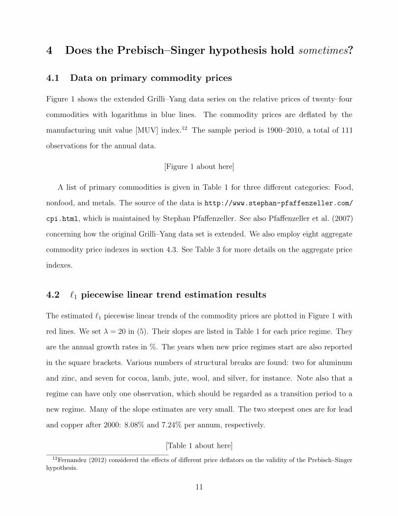
Figure 1 shows the extended Grilli–Yang data series on the relative prices of twenty–four

commodities with logarithms in blue lines. The commodity prices are deflated by the

manufacturing unit value [MUV] index.12 The sample period is 1900–2010, a total of 111

observations for the annual data.

[Figure 1 about here]

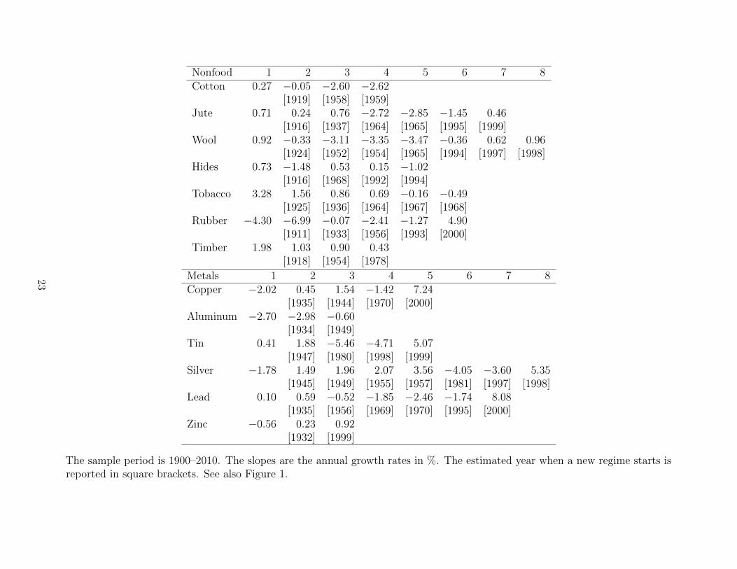
A list of primary commodities is given in Table 1 for three different categories: Food,

nonfood, and metals. The source of the data is http://www.stephan-pfaffenzeller.com/

cpi.html, which is maintained by Stephan Pfaffenzeller. See also Pfaffenzeller et al. (2007)

concerning how the original Grilli–Yang data set is extended. We also employ eight aggregate

commodity price indexes in section 4.3. See Table 3 for more details on the aggregate price

indexes.

4.2 `1 piecewise linear trend estimation results

The estimated `1 piecewise linear trends of the commodity prices are plotted in Figure 1 with

red lines. We set λ = 20 in (5). Their slopes are listed in Table 1 for each price regime. They

are the annual growth rates in %. The years when new price regimes start are also reported

in the square brackets. Various numbers of structural breaks are found: two for aluminum

and zinc, and seven for cocoa, lamb, jute, wool, and silver, for instance. Note also that a

regime can have only one observation, which should be regarded as a transition period to a

new regime. Many of the slope estimates are very small. The two steepest ones are for lead

and copper after 2000: 8.08% and 7.24% per annum, respectively.

[Table 1 about here]

12Fernandez (2012) considered the effects of different price deflators on the validity of the Prebisch–Singerhypothesis.

11

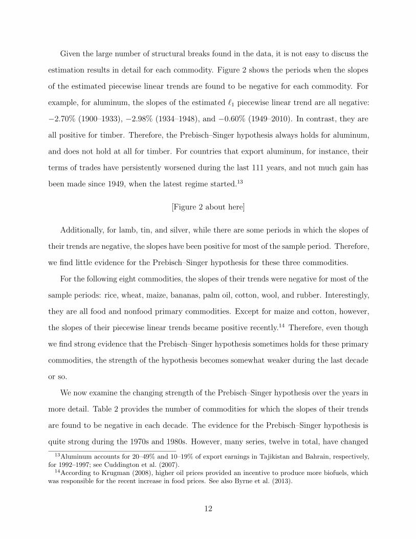
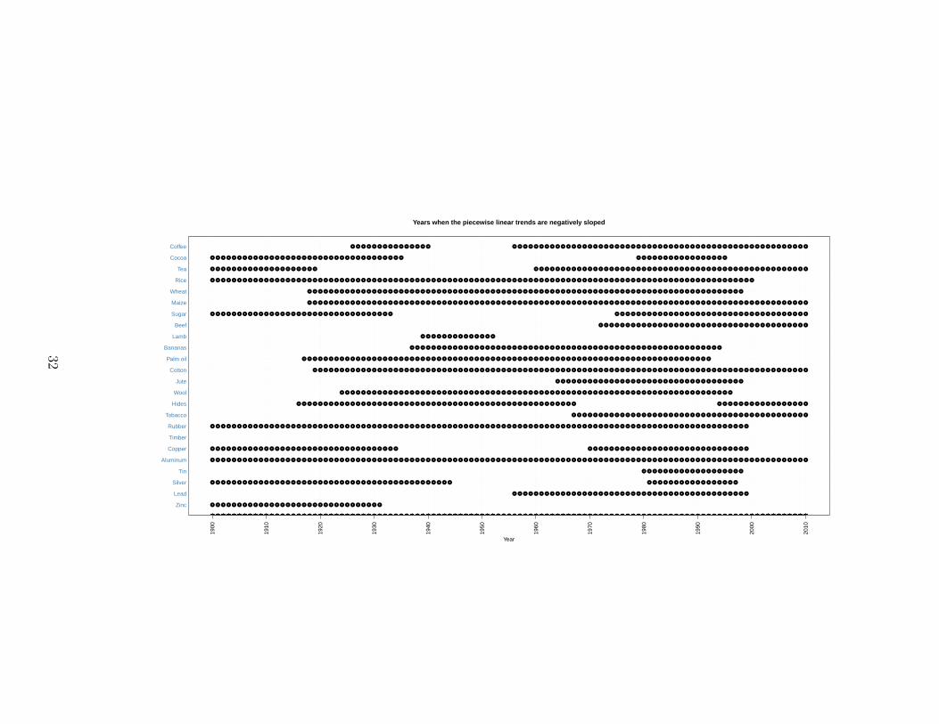
Given the large number of structural breaks found in the data, it is not easy to discuss the

estimation results in detail for each commodity. Figure 2 shows the periods when the slopes

of the estimated piecewise linear trends are found to be negative for each commodity. For

example, for aluminum, the slopes of the estimated `1 piecewise linear trend are all negative:

−2.70% (1900–1933), −2.98% (1934–1948), and −0.60% (1949–2010). In contrast, they are

all positive for timber. Therefore, the Prebisch–Singer hypothesis always holds for aluminum,

and does not hold at all for timber. For countries that export aluminum, for instance, their

terms of trades have persistently worsened during the last 111 years, and not much gain has

been made since 1949, when the latest regime started.13

[Figure 2 about here]

Additionally, for lamb, tin, and silver, while there are some periods in which the slopes of

their trends are negative, the slopes have been positive for most of the sample period. Therefore,

we find little evidence for the Prebisch–Singer hypothesis for these three commodities.

For the following eight commodities, the slopes of their trends were negative for most of the

sample periods: rice, wheat, maize, bananas, palm oil, cotton, wool, and rubber. Interestingly,

they are all food and nonfood primary commodities. Except for maize and cotton, however,

the slopes of their piecewise linear trends became positive recently.14 Therefore, even though

we find strong evidence that the Prebisch–Singer hypothesis sometimes holds for these primary

commodities, the strength of the hypothesis becomes somewhat weaker during the last decade

or so.

We now examine the changing strength of the Prebisch–Singer hypothesis over the years in

more detail. Table 2 provides the number of commodities for which the slopes of their trends

are found to be negative in each decade. The evidence for the Prebisch–Singer hypothesis is

quite strong during the 1970s and 1980s. However, many series, twelve in total, have changed

13Aluminum accounts for 20–49% and 10–19% of export earnings in Tajikistan and Bahrain, respectively,for 1992–1997; see Cuddington et al. (2007).

14According to Krugman (2008), higher oil prices provided an incentive to produce more biofuels, whichwas responsible for the recent increase in food prices. See also Byrne et al. (2013).

12

the signs of their trend functions from negative to positive since 1992. For example, rice and

rubber, which had negatively sloped piecewise linear trends for about 100 years, now have

positively sloped trends. Only nine prices are found to have negatively sloped trends since

2000, and evidence for the Prebisch–Singer hypothesis has recently become much weaker.

[Table 2 about here]

In 1950, when the works by Prebisch and Singer were published simultaneously and

independently, negatively sloped trends were observed in less than half of the twenty–four

commodities that later comprised the Grilli–Yang data set. Singer (1984) noted, however,

that his 1950 thesis was not unduly influenced by the rising trend of the preceding ten years,

but by long–term decline in the 1870–1939 period. Given the lack of trends in subsequent

years, Williamson (2012) declared that the Prebisch–Singer announcement of secular decline

of relative primary commodity prices was premature. At the time when Grilli and Yang

(1988) tested the Prebisch–Singer hypothesis with their new data set, many commodities,

which had exhibited positively sloped trends for a long time, had recently turned around into

negatively sloped ones: cocoa, sugar, beef, jute, copper, tin, and silver.

Overall, we may conclude that the Prebisch–Singer hypothesis holds sometimes, but not

always for most of the primary commodities in the extended Grilli–Yang data set, ending at

2010. The strength of the Prebisch–Singer hypothesis has become substantially weaker in

recent years, as the relative prices of many primary commodities increased substantially since

about 2000.

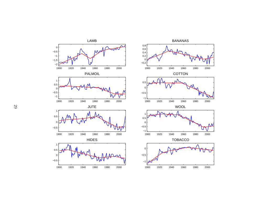
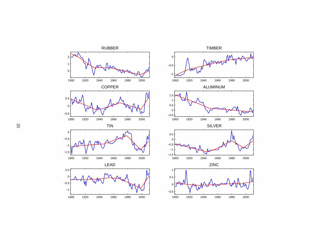
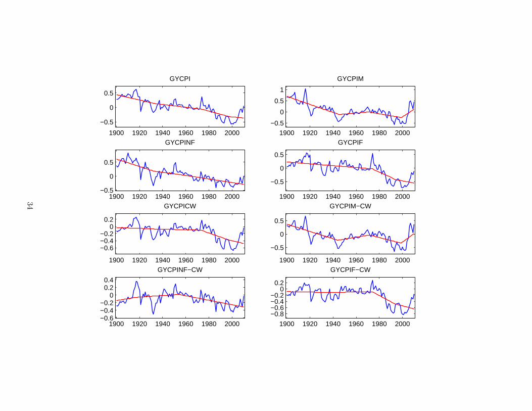
4.3 Results from aggregate commodity prices

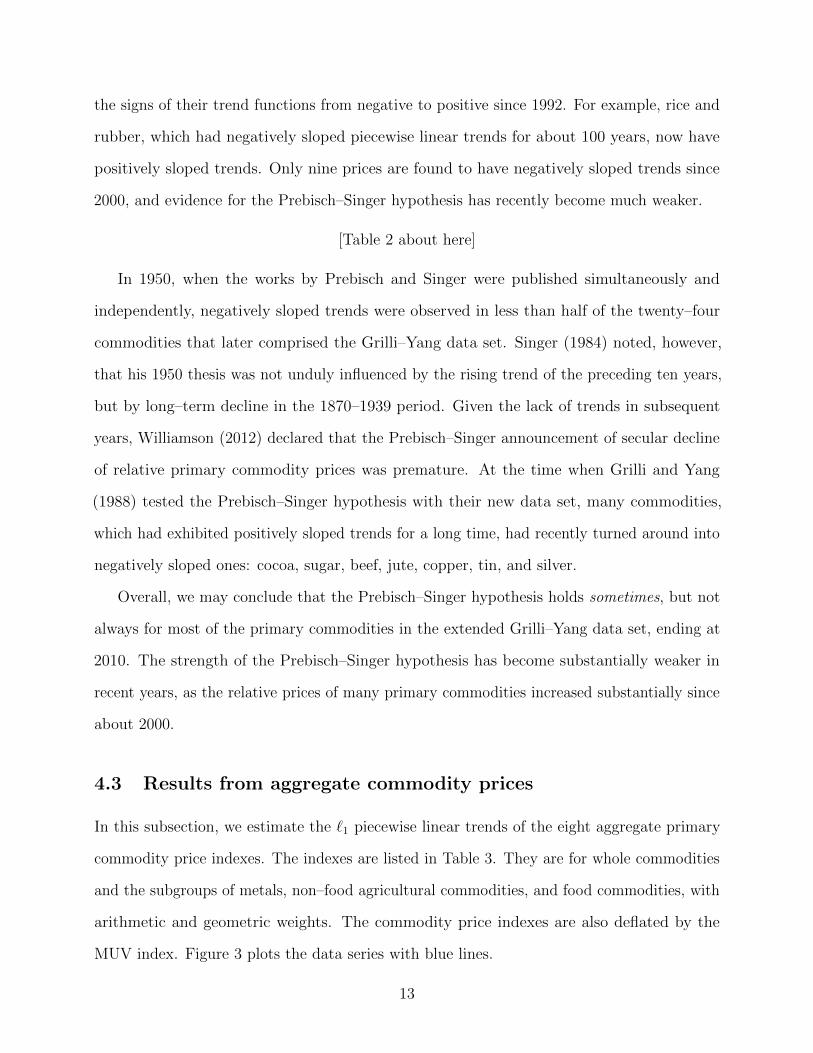
In this subsection, we estimate the `1 piecewise linear trends of the eight aggregate primary

commodity price indexes. The indexes are listed in Table 3. They are for whole commodities

and the subgroups of metals, non–food agricultural commodities, and food commodities, with

arithmetic and geometric weights. The commodity price indexes are also deflated by the

MUV index. Figure 3 plots the data series with blue lines.

13

[Table 3 and Figure 3 about here]

The `1 piecewise linear trend filtering results are presented in Table 4, where the estimated

slopes of the trends and structural break dates are reported. We again set λ = 20 in (5).

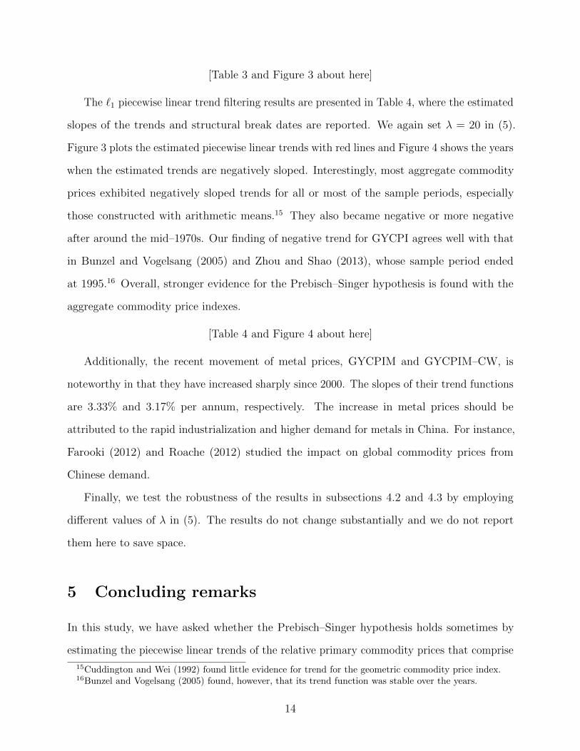
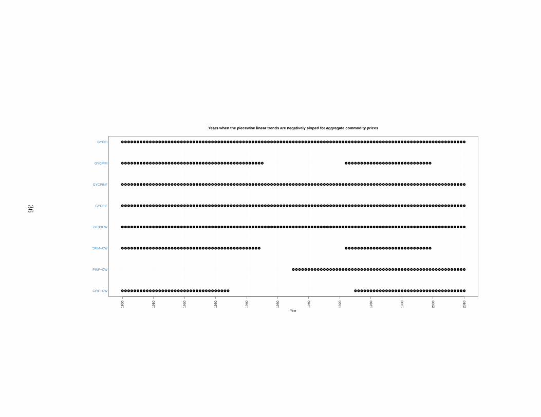
Figure 3 plots the estimated piecewise linear trends with red lines and Figure 4 shows the years

when the estimated trends are negatively sloped. Interestingly, most aggregate commodity

prices exhibited negatively sloped trends for all or most of the sample periods, especially

those constructed with arithmetic means.15 They also became negative or more negative

after around the mid–1970s. Our finding of negative trend for GYCPI agrees well with that

in Bunzel and Vogelsang (2005) and Zhou and Shao (2013), whose sample period ended

at 1995.16 Overall, stronger evidence for the Prebisch–Singer hypothesis is found with the

aggregate commodity price indexes.

[Table 4 and Figure 4 about here]

Additionally, the recent movement of metal prices, GYCPIM and GYCPIM–CW, is

noteworthy in that they have increased sharply since 2000. The slopes of their trend functions

are 3.33% and 3.17% per annum, respectively. The increase in metal prices should be

attributed to the rapid industrialization and higher demand for metals in China. For instance,

Farooki (2012) and Roache (2012) studied the impact on global commodity prices from

Chinese demand.

Finally, we test the robustness of the results in subsections 4.2 and 4.3 by employing

different values of λ in (5). The results do not change substantially and we do not report

them here to save space.

5 Concluding remarks

In this study, we have asked whether the Prebisch–Singer hypothesis holds sometimes by

estimating the piecewise linear trends of the relative primary commodity prices that comprise

15Cuddington and Wei (1992) found little evidence for trend for the geometric commodity price index.16Bunzel and Vogelsang (2005) found, however, that its trend function was stable over the years.

14

the famous Grilli–Yang data set. When the slope of the trend is negative, we say that the

hypothesis holds locally in the regime.

We apply the newly proposed `1 trend filtering by Kim et al. (2009) to estimate the trends.

A notable feature of `1 trend filtering is that it produces a piecewise linear trend function

of time. The number and dates of structural breaks are not known a priori, and they are

simultaneously estimated with the piecewise linear trends.

We find little evidence that the Prebisch–Singer hypothesis always holds in the extended

Grilli–Yang primary commodity price data, ending at 2010. For most primary commodities,

however, we find that their piecewise linear trends are negatively sloped during some of the

sample periods and that the Prebisch–Singer hypothesis holds sometimes. The strength of

the hypothesis has become substantially weaker in recent years, as the prices of many primary

commodities have increased since around 2000.

15

References

Arezki, Rabah, Kaddour Hadri, Eiji Kurozumi, and Yao Rao, 2012, Testing the Prebisch–Singer

hypothesis using second–generation panel data stationarity tests with a break, Economics

Letters, 117, 814–816

Balagtas, Joseph V. and Matthew T. Holt, 2009, The commodity terms of trade, unit

roots, and nonlinear alternatives: a smooth transition approach, American Journal of Agricul-

tural Economics, 91, 87–105

Belloni, Alexandre and Victor Chernozhukov, 2011, High dimensional sparse economet-

ric models: An introduction, in Inverse Problems and High–Dimensional Estimation, P.

Alquier, E. Gautier, and G. Stoltz, (Eds.), 121–156, Lecture Notes in Statistics, volume 203,

Springer Berlin Heidelberg

Brinkhuis, Jan and Vladimir Tikhomirov, 2005, Optimization: Insights and Applications,

Princeton University Press

Bunzel, Helle and Timothy J. Vogelsang, 2005, Powerful trend function tests that are robust

to strong serial correlation, with an application to the Prebisch–Singer hypothesis, Journal of

Business and Economic Statistics, 23, 381–394

Byrne, Joseph P., Giorgio Fazio, and Norbert Fiess, 2013, Primary commodity prices: Co–

movements, common factors and fundamentals, Journal of Development Economics, 101, 16–26

Cashin, Paul and John McDermott, 2002, The long–run behavior of commodity prices:

Small trends and big volatility, IMF Staff Papers, 49, 175–199

16

Cuddington, John T., Rodney Ludema, and Shamila A. Jayasuriya, 2007, Prebisch–Singer

redux, in Natural Resources: Neither Curse nor Destiny, D. Lederman and W.F. Maloney

(Eds.), 103–140, The World Bank/Stanford University Press

Cuddington, John T. and Hong Wei, 1992, An empirical analysis of real commodity price

trends: aggregation, model selection and implications, Estudios Economicos, 7, 159–179

Deaton, Angus, 1999, Commodity prices and growth in Africa, Journal of Economic Perspec-

tives, 13, 23–40

Farooki, Masuma Zareen, 2012, China’s metals demand and commodity prices: a case

of disruptive development? European Journal of Development Research, 24, 56–70

Fernandez, Viviana, 2012, Trends in real commodity prices: How real is real? Resources

Policy, 37, 30–47

Ghoshray, Atanu, 2011, A reexamination of trends in primary commodity prices, Jour-

nal of Development Economics, 95, 242–251

Grant, Michael and Stephen Boyd, 2008, Graph implementations for nonsmooth convex

programs, in Recent Advances in Learning and Control (a tribute to M. Vidyasagar), V.

Blondel, S. Boyd, and H. Kimura (Eds.), 95–110, Lecture Notes in Control and Information

Sciences, Springer, http://stanford.edu/~boyd/graph_dcp.html

Grant, Michael and Stephen Boyd, 2011, CVX: Matlab software for disciplined convex

programming, version 1.21, http://stanford.edu/~boyd/cvx

17

Grilli, Enzo and Maw Cheng Yang, 1988, Primary commodity prices, manufactured goods

prices, and the terms of trade of developing countries: What the long run shows, The World

Bank Economic Review, 2, 1–47

Harvey, David I., Neil M. Kellard, Jakob B, Madsen, and Mark E. Wohar, 2010, The Prebisch–

Singer hypothesis: Four centuries of evidence, Review of Economics and Statistics, 92, 367–377

Harvey, David I., Neil M. Kellard, Jakob B, Madsen, and Mark E. Wohar, 2012, Erra-

tum: The Prebisch–Singer hypothesis: Four centuries of evidence, manuscript

Harvey, David I., Stephen J. Leybourne, and A.M. Robert Taylor, 2011, Testing for unit roots

and the impact of quadratic trends, with an application to relative primary commodity prices,

Econometric Reviews, 30, 514–547

Hodrick, Robert J. and Edward C. Prescott, 1997, Postwar U.S. business cycles: An empirical

investigation, Journal of Money, Credit and Banking, 29, 1–16

Kellard, Neil and Mark E. Wohar, 2006, On the prevalence of trends in primary com-

modity prices, Journal of Development Economics, 79, 146–167

Kim, Seung-Jean, Kwangmoo Koh, Stephen Boyd, and Dimitry Gorinevsky, 2009, `1 trend

filtering, SIAM Review, 51, 339–360

Kim, Tae-Hwan, Stephan Pfaffenzeller, Tony Rayner, and Paul Newbold, 2003, Testing

for linear trend with applications to relative primary commodity prices, Journal of Time

Series Analysis, 24, 539–551

18

Krugman, Paul, 2008, Running out of planet to exploit, New York Times Op-Ed Column,

April 21, available at http://www.nytimes.com/2008/04/21/opinion/21krugman.html

Leon, Javier and Raimundo Soto, 1997, Structural breaks and long–run trends in com-

modity prices, Journal of International Development, 9, 347–366

Lumsdaine, Robin L. and David H. Papell, 1997, Multiple trend breaks and the unit root

hypothesis, Review of Economics and Statistics, 79, 212–218

Ocampo, Jose and Mariangela Parra-Lancourt, 2010, The terms of trade for commodities

since the mid–19th century, Journal of Iberian and Latin American Economic History, 28, 11–43

OECD, 2012, OECD system of composite leading indicators, manuscript available at http:

//www.oecd.org/dataoecd/26/39/41629509.pdf

Otero, Jesus and Ana Marıa Iregui, 2011, The long–run behavior of the terms of trade

between primary commodities and manufactures, manuscript

Paige, Robert L. and A. Alexandre Trindade, 2010, The Hodrick–Prescott filter: A spe-

cial case of penalized spline smoothing, Electronic Journal of Statistics, 4, 856–874

Pfaffenzeller, Stephan, Paul Newbold, and Anthony Rayner, 2007, A short note on up-

dating the Grilli and Yang commodity price index, The World Bank Economic Review, 21,

1–13

Prebisch, Raul, 1950, The Economic Development of Latin America and its Principal Problems,

New York: United Nations

19

Roache, Shaun K., 2012, China’s impact on world commodity markets, IMF working paper

12/115

Singer, Hans W., 1950, The distribution of gains between investing and borrowing countries,

American Economic Review, 40, 473–485

Singer, Hans W., 1984, The terms of trade controversy and the evolution of soft financ-

ing: Early years in the U.N., in Pioneers in Development, G.M. Meier and D. Seers (Eds.),

275–303, The World Bank/Oxford University Press

Tibshirani, Robert, 1996, Regression shrinkage and selection via the lasso, Journal of the

Royal Statistical Society, Series B, 58, 267–288

Tibshirani, Ryan J. and Jonathan Taylor, 2011, The solution path of the generalized lasso,

Annals of Statistics, 39, 1335–1371

Tilton, John E., 2012, The terms of trade debate and the policy implications for primary

product producers, forthcoming at Resources Policy

Williamson, Jeffrey G., 2012, Commodity prices over two centuries: Trends, volatility, and

impact, Annual Review of Resource Economics, 4, 185–206

Yamada, Hiroshi, 2011, A note on band–pass filters based on the Hodrick–Prescott filter and

the OECD system of composite leading indicators, OECD Journal: Journal of Business Cycle

Measurement and Analysis, 2011, 105–109

20

Yamada, Hiroshi and Lan Jin, 2012, Japan’s output gap estimation and `1 trend filter-

ing, forthcoming at Empirical Economics

Yamada, Hiroshi and Gawon Yoon, 2012a, Piecewise quadratic trend in U.S. unemploy-

ment rate, manuscript

Yamada, Hiroshi and Gawon Yoon, 2012b, High–low–high? Occasional level shifts in U.S.

productivity, manuscript

Yang, Chao-Hsiang, Chi-Tai Lin, and Yu-Sheng Kao, 2012, Exploring stationarity and

structural breaks in commodity prices by the panel data model, Applied Economics Letters,

19, 353–361

Zanias, George P., 2005, Testing for trends in the terms of trade between primary com-

modities and manufactured goods, Journal of Development Economics, 78, 49–59

Zhou, Zhou and Xiaofeng Shao, 2013, Inference for linear models with dependent errors,

Journal of the Royal Statistical Society, Series B, 75, 323–343

21

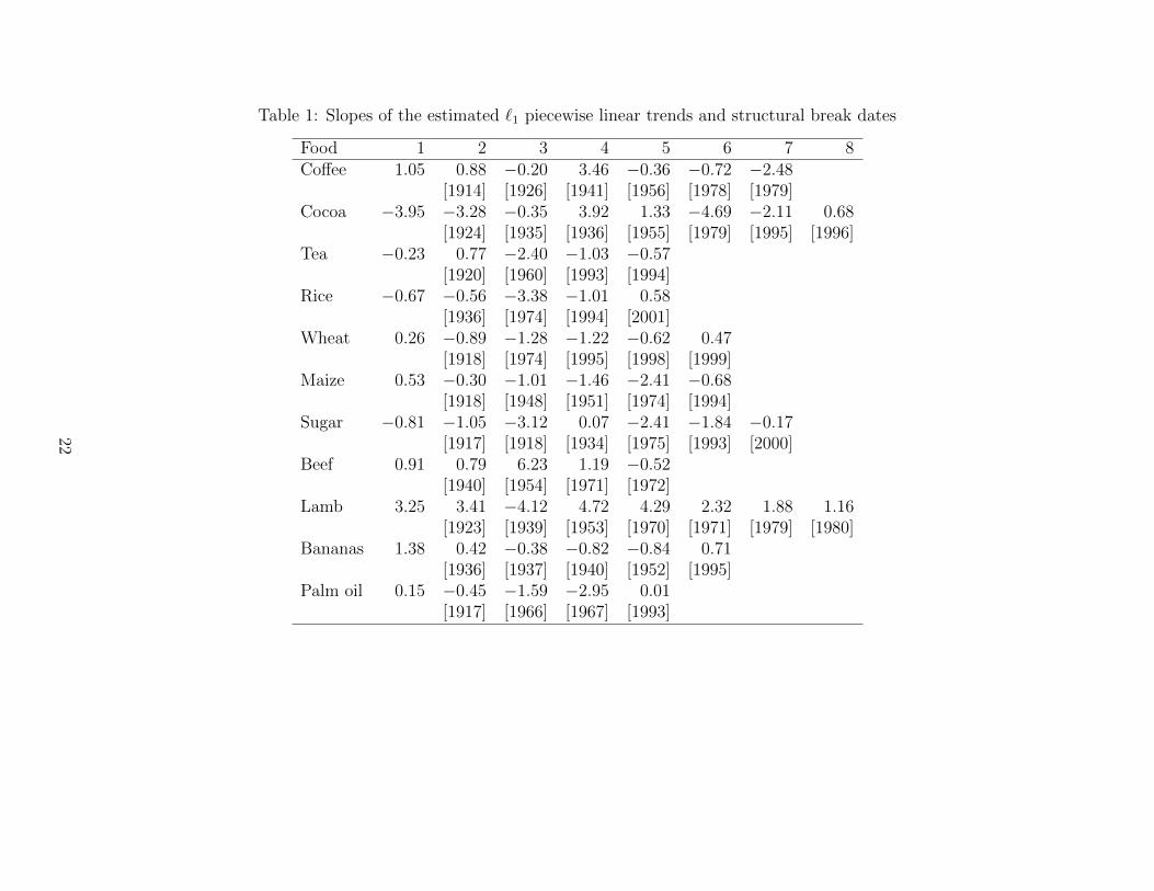
Table 1: Slopes of the estimated `1 piecewise linear trends and structural break dates

Food 1 2 3 4 5 6 7 8Coffee 1.05 0.88 −0.20 3.46 −0.36 −0.72 −2.48

[1914] [1926] [1941] [1956] [1978] [1979]Cocoa −3.95 −3.28 −0.35 3.92 1.33 −4.69 −2.11 0.68

[1924] [1935] [1936] [1955] [1979] [1995] [1996]Tea −0.23 0.77 −2.40 −1.03 −0.57

[1920] [1960] [1993] [1994]Rice −0.67 −0.56 −3.38 −1.01 0.58

[1936] [1974] [1994] [2001]Wheat 0.26 −0.89 −1.28 −1.22 −0.62 0.47

[1918] [1974] [1995] [1998] [1999]Maize 0.53 −0.30 −1.01 −1.46 −2.41 −0.68

[1918] [1948] [1951] [1974] [1994]Sugar −0.81 −1.05 −3.12 0.07 −2.41 −1.84 −0.17

[1917] [1918] [1934] [1975] [1993] [2000]Beef 0.91 0.79 6.23 1.19 −0.52

[1940] [1954] [1971] [1972]Lamb 3.25 3.41 −4.12 4.72 4.29 2.32 1.88 1.16

[1923] [1939] [1953] [1970] [1971] [1979] [1980]Bananas 1.38 0.42 −0.38 −0.82 −0.84 0.71

[1936] [1937] [1940] [1952] [1995]Palm oil 0.15 −0.45 −1.59 −2.95 0.01

[1917] [1966] [1967] [1993]

22

Nonfood 1 2 3 4 5 6 7 8Cotton 0.27 −0.05 −2.60 −2.62

[1919] [1958] [1959]Jute 0.71 0.24 0.76 −2.72 −2.85 −1.45 0.46

[1916] [1937] [1964] [1965] [1995] [1999]Wool 0.92 −0.33 −3.11 −3.35 −3.47 −0.36 0.62 0.96

[1924] [1952] [1954] [1965] [1994] [1997] [1998]Hides 0.73 −1.48 0.53 0.15 −1.02

[1916] [1968] [1992] [1994]Tobacco 3.28 1.56 0.86 0.69 −0.16 −0.49

[1925] [1936] [1964] [1967] [1968]Rubber −4.30 −6.99 −0.07 −2.41 −1.27 4.90

[1911] [1933] [1956] [1993] [2000]Timber 1.98 1.03 0.90 0.43

[1918] [1954] [1978]

Metals 1 2 3 4 5 6 7 8Copper −2.02 0.45 1.54 −1.42 7.24

[1935] [1944] [1970] [2000]Aluminum −2.70 −2.98 −0.60

[1934] [1949]Tin 0.41 1.88 −5.46 −4.71 5.07

[1947] [1980] [1998] [1999]Silver −1.78 1.49 1.96 2.07 3.56 −4.05 −3.60 5.35

[1945] [1949] [1955] [1957] [1981] [1997] [1998]Lead 0.10 0.59 −0.52 −1.85 −2.46 −1.74 8.08

[1935] [1956] [1969] [1970] [1995] [2000]Zinc −0.56 0.23 0.92

[1932] [1999]

The sample period is 1900–2010. The slopes are the annual growth rates in %. The estimated year when a new regime starts isreported in square brackets. See also Figure 1.

23

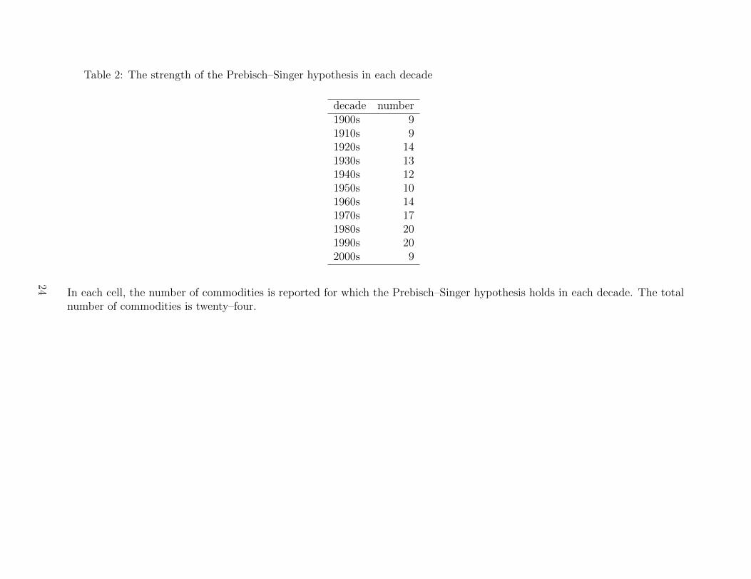
Table 2: The strength of the Prebisch–Singer hypothesis in each decade

decade number1900s 91910s 91920s 141930s 131940s 121950s 101960s 141970s 171980s 201990s 202000s 9

In each cell, the number of commodities is reported for which the Prebisch–Singer hypothesis holds in each decade. The totalnumber of commodities is twenty–four.

24

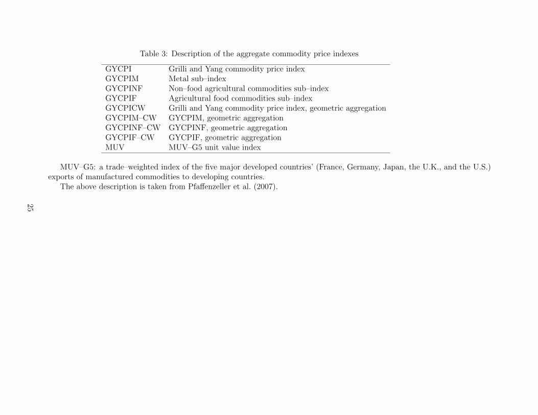
Table 3: Description of the aggregate commodity price indexes

GYCPI Grilli and Yang commodity price indexGYCPIM Metal sub–indexGYCPINF Non–food agricultural commodities sub–indexGYCPIF Agricultural food commodities sub–indexGYCPICW Grilli and Yang commodity price index, geometric aggregationGYCPIM–CW GYCPIM, geometric aggregationGYCPINF–CW GYCPINF, geometric aggregationGYCPIF–CW GYCPIF, geometric aggregationMUV MUV–G5 unit value index

MUV–G5: a trade–weighted index of the five major developed countries’ (France, Germany, Japan, the U.K., and the U.S.)exports of manufactured commodities to developing countries.

The above description is taken from Pfaffenzeller et al. (2007).

25

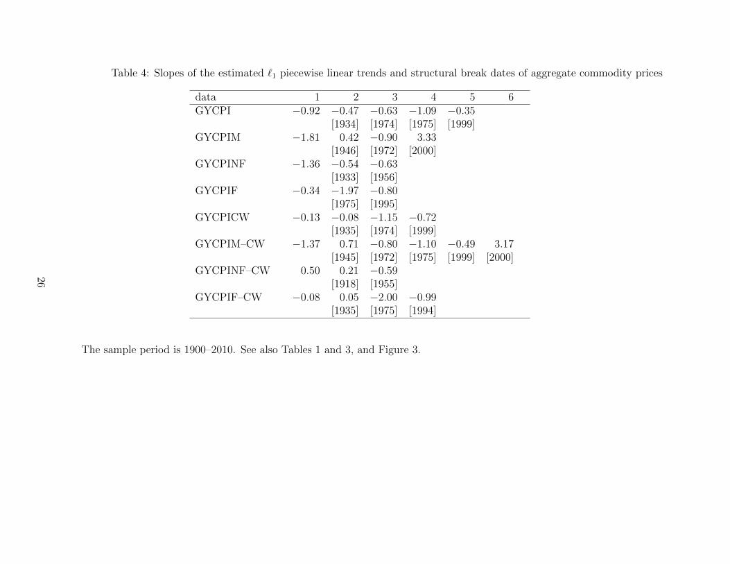
Table 4: Slopes of the estimated `1 piecewise linear trends and structural break dates of aggregate commodity prices

data 1 2 3 4 5 6GYCPI −0.92 −0.47 −0.63 −1.09 −0.35

[1934] [1974] [1975] [1999]GYCPIM −1.81 0.42 −0.90 3.33

[1946] [1972] [2000]GYCPINF −1.36 −0.54 −0.63

[1933] [1956]GYCPIF −0.34 −1.97 −0.80

[1975] [1995]GYCPICW −0.13 −0.08 −1.15 −0.72

[1935] [1974] [1999]GYCPIM–CW −1.37 0.71 −0.80 −1.10 −0.49 3.17

[1945] [1972] [1975] [1999] [2000]GYCPINF–CW 0.50 0.21 −0.59

[1918] [1955]GYCPIF–CW −0.08 0.05 −2.00 −0.99

[1935] [1975] [1994]

The sample period is 1900–2010. See also Tables 1 and 3, and Figure 3.

26

Note for Figure 1

The blue line shows the data and the red line plots the estimated `1 piecewise linear trend.

See also Table 1.

27

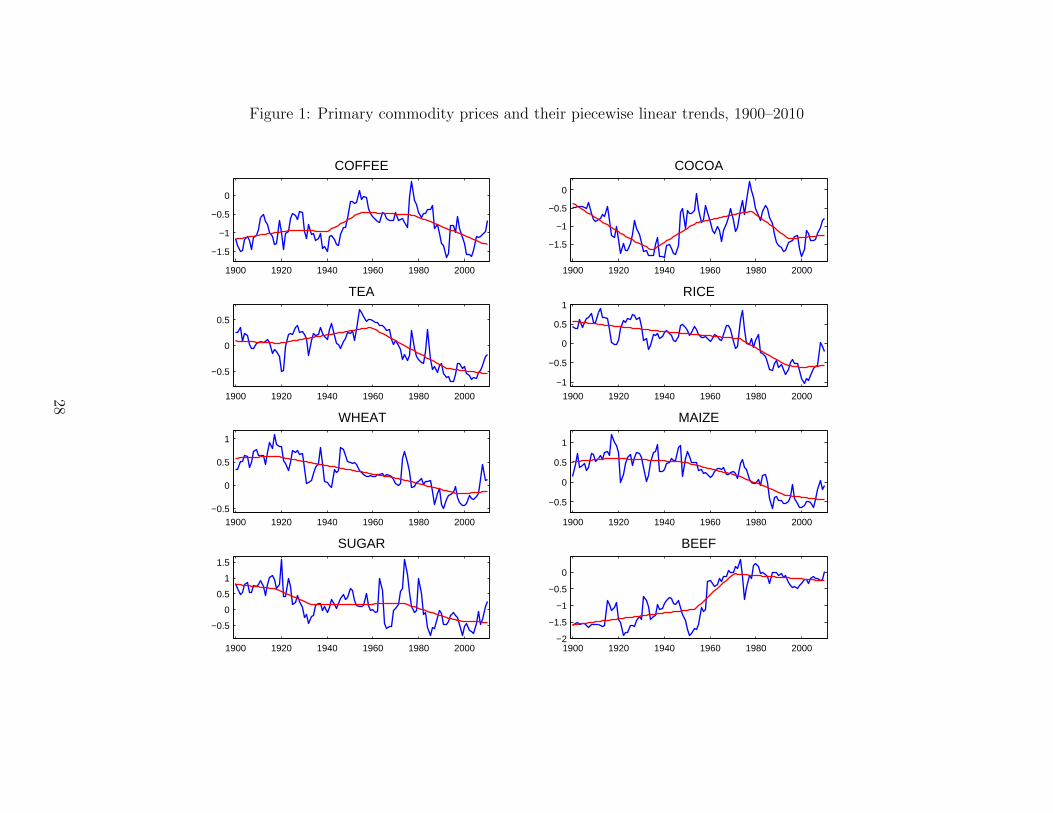
Figure 1: Primary commodity prices and their piecewise linear trends, 1900–2010

1900 1920 1940 1960 1980 2000

−1.5

−1

−0.5

0

COFFEE

1900 1920 1940 1960 1980 2000

−1.5

−1

−0.5

0

COCOA

1900 1920 1940 1960 1980 2000

−0.5

0

0.5

TEA

1900 1920 1940 1960 1980 2000

−1

−0.5

0

0.5

1RICE

1900 1920 1940 1960 1980 2000−0.5

0

0.5

1

WHEAT

1900 1920 1940 1960 1980 2000

−0.5

0

0.5

1

MAIZE

1900 1920 1940 1960 1980 2000

−0.5

0

0.5

1

1.5

SUGAR

1900 1920 1940 1960 1980 2000−2

−1.5

−1

−0.5

0

BEEF

28

1900 1920 1940 1960 1980 2000

−2

−1.5

−1

−0.5

0

LAMB

1900 1920 1940 1960 1980 2000

−0.20

0.20.40.60.8

BANANAS

1900 1920 1940 1960 1980 2000

−1

−0.5

0

0.5

1

PALMOIL

1900 1920 1940 1960 1980 2000−1

−0.5

0

0.5

COTTON

1900 1920 1940 1960 1980 2000

−0.5

0

0.5

1

JUTE

1900 1920 1940 1960 1980 2000−1

−0.5

0

0.5

1

WOOL

1900 1920 1940 1960 1980 2000

−0.5

0

0.5

1

HIDES

1900 1920 1940 1960 1980 2000

−1

−0.5

0

TOBACCO

29

1900 1920 1940 1960 1980 2000

0

1

2

RUBBER

1900 1920 1940 1960 1980 2000

−1

−0.5

0

TIMBER

1900 1920 1940 1960 1980 2000

−0.5

0

0.5

COPPER

1900 1920 1940 1960 1980 2000−0.5

0

0.5

1

1.5

ALUMINUM

1900 1920 1940 1960 1980 2000

−1.5

−1

−0.5

0

TIN

1900 1920 1940 1960 1980 2000−1.5

−1

−0.5

0

0.5

SILVER

1900 1920 1940 1960 1980 2000

−1

−0.5

0

0.5

LEAD

1900 1920 1940 1960 1980 2000

−0.5

0

0.5

1

ZINC

30

Figure 2: Years when the piecewise linear trends are negatively sloped

The dotted lines indicate the years when the `1 piecewise linear trends are negatively sloped

for each commodity.

31

● ● ● ● ● ● ● ● ● ● ● ● ● ● ● ● ● ● ● ● ● ● ● ● ● ●

● ● ● ● ● ● ● ● ● ● ● ● ● ● ●

● ● ● ● ● ● ● ● ● ● ● ● ● ● ●

● ● ● ● ● ● ● ● ● ● ● ● ● ● ● ● ● ● ● ● ● ● ● ● ● ● ● ● ● ● ● ● ● ● ● ● ● ● ● ● ● ● ● ● ● ● ● ● ● ● ● ● ● ● ●

Years when the piecewise linear trends are negatively sloped

Year

1900

1910

1920

1930

1940

1950

1960

1970

1980

1990

2000

2010

Coffee

● ● ● ● ● ● ● ● ● ● ● ● ● ● ● ● ● ● ● ● ● ● ● ● ● ● ● ● ● ● ● ● ● ● ● ●

● ● ● ● ● ● ● ● ● ● ● ● ● ● ● ● ● ● ● ● ● ● ● ● ● ● ● ● ● ● ● ● ● ● ● ● ● ● ● ● ● ● ●

● ● ● ● ● ● ● ● ● ● ● ● ● ● ● ● ●

● ● ● ● ● ● ● ● ● ● ● ● ● ● ●

Cocoa

● ● ● ● ● ● ● ● ● ● ● ● ● ● ● ● ● ● ● ●

● ● ● ● ● ● ● ● ● ● ● ● ● ● ● ● ● ● ● ● ● ● ● ● ● ● ● ● ● ● ● ● ● ● ● ● ● ● ● ●

● ● ● ● ● ● ● ● ● ● ● ● ● ● ● ● ● ● ● ● ● ● ● ● ● ● ● ● ● ● ● ● ● ● ● ● ● ● ● ● ● ● ● ● ● ● ● ● ● ● ●Tea

● ● ● ● ● ● ● ● ● ● ● ● ● ● ● ● ● ● ● ● ● ● ● ● ● ● ● ● ● ● ● ● ● ● ● ● ● ● ● ● ● ● ● ● ● ● ● ● ● ● ● ● ● ● ● ● ● ● ● ● ● ● ● ● ● ● ● ● ● ● ● ● ● ● ● ● ● ● ● ● ● ● ● ● ● ● ● ● ● ● ● ● ● ● ● ● ● ● ● ● ●

● ● ● ● ● ● ● ● ● ●

Rice

● ● ● ● ● ● ● ● ● ● ● ● ● ● ● ● ● ●

● ● ● ● ● ● ● ● ● ● ● ● ● ● ● ● ● ● ● ● ● ● ● ● ● ● ● ● ● ● ● ● ● ● ● ● ● ● ● ● ● ● ● ● ● ● ● ● ● ● ● ● ● ● ● ● ● ● ● ● ● ● ● ● ● ● ● ● ● ● ● ● ● ● ● ● ● ● ● ● ●

● ● ● ● ● ● ● ● ● ● ● ●

Wheat

● ● ● ● ● ● ● ● ● ● ● ● ● ● ● ● ● ●

● ● ● ● ● ● ● ● ● ● ● ● ● ● ● ● ● ● ● ● ● ● ● ● ● ● ● ● ● ● ● ● ● ● ● ● ● ● ● ● ● ● ● ● ● ● ● ● ● ● ● ● ● ● ● ● ● ● ● ● ● ● ● ● ● ● ● ● ● ● ● ● ● ● ● ● ● ● ● ● ● ● ● ● ● ● ● ● ● ● ● ● ●Maize

● ● ● ● ● ● ● ● ● ● ● ● ● ● ● ● ● ● ● ● ● ● ● ● ● ● ● ● ● ● ● ● ● ●

● ● ● ● ● ● ● ● ● ● ● ● ● ● ● ● ● ● ● ● ● ● ● ● ● ● ● ● ● ● ● ● ● ● ● ● ● ● ● ● ●

● ● ● ● ● ● ● ● ● ● ● ● ● ● ● ● ● ● ● ● ● ● ● ● ● ● ● ● ● ● ● ● ● ● ● ●Sugar

● ● ● ● ● ● ● ● ● ● ● ● ● ● ● ● ● ● ● ● ● ● ● ● ● ● ● ● ● ● ● ● ● ● ● ● ● ● ● ● ● ● ● ● ● ● ● ● ● ● ● ● ● ● ● ● ● ● ● ● ● ● ● ● ● ● ● ● ● ● ● ●

● ● ● ● ● ● ● ● ● ● ● ● ● ● ● ● ● ● ● ● ● ● ● ● ● ● ● ● ● ● ● ● ● ● ● ● ● ● ●Beef

● ● ● ● ● ● ● ● ● ● ● ● ● ● ● ● ● ● ● ● ● ● ● ● ● ● ● ● ● ● ● ● ● ● ● ● ● ● ●

● ● ● ● ● ● ● ● ● ● ● ● ● ●

● ● ● ● ● ● ● ● ● ● ● ● ● ● ● ● ● ● ● ● ● ● ● ● ● ● ● ● ● ● ● ● ● ● ● ● ● ● ● ● ● ● ● ● ● ● ● ● ● ● ● ● ● ● ● ● ● ●

Lamb

● ● ● ● ● ● ● ● ● ● ● ● ● ● ● ● ● ● ● ● ● ● ● ● ● ● ● ● ● ● ● ● ● ● ● ● ●

● ● ● ● ● ● ● ● ● ● ● ● ● ● ● ● ● ● ● ● ● ● ● ● ● ● ● ● ● ● ● ● ● ● ● ● ● ● ● ● ● ● ● ● ● ● ● ● ● ● ● ● ● ● ● ● ● ●

● ● ● ● ● ● ● ● ● ● ● ● ● ● ● ●

Bananas

● ● ● ● ● ● ● ● ● ● ● ● ● ● ● ● ●

● ● ● ● ● ● ● ● ● ● ● ● ● ● ● ● ● ● ● ● ● ● ● ● ● ● ● ● ● ● ● ● ● ● ● ● ● ● ● ● ● ● ● ● ● ● ● ● ● ● ● ● ● ● ● ● ● ● ● ● ● ● ● ● ● ● ● ● ● ● ● ● ● ● ● ●

● ● ● ● ● ● ● ● ● ● ● ● ● ● ● ● ● ●

Palm oil

● ● ● ● ● ● ● ● ● ● ● ● ● ● ● ● ● ● ●

● ● ● ● ● ● ● ● ● ● ● ● ● ● ● ● ● ● ● ● ● ● ● ● ● ● ● ● ● ● ● ● ● ● ● ● ● ● ● ● ● ● ● ● ● ● ● ● ● ● ● ● ● ● ● ● ● ● ● ● ● ● ● ● ● ● ● ● ● ● ● ● ● ● ● ● ● ● ● ● ● ● ● ● ● ● ● ● ● ● ● ●Cotton

● ● ● ● ● ● ● ● ● ● ● ● ● ● ● ● ● ● ● ● ● ● ● ● ● ● ● ● ● ● ● ● ● ● ● ● ● ● ● ● ● ● ● ● ● ● ● ● ● ● ● ● ● ● ● ● ● ● ● ● ● ● ● ●

● ● ● ● ● ● ● ● ● ● ● ● ● ● ● ● ● ● ● ● ● ● ● ● ● ● ● ● ● ● ● ● ● ● ●

● ● ● ● ● ● ● ● ● ● ● ●

Jute

● ● ● ● ● ● ● ● ● ● ● ● ● ● ● ● ● ● ● ● ● ● ● ●

● ● ● ● ● ● ● ● ● ● ● ● ● ● ● ● ● ● ● ● ● ● ● ● ● ● ● ● ● ● ● ● ● ● ● ● ● ● ● ● ● ● ● ● ● ● ● ● ● ● ● ● ● ● ● ● ● ● ● ● ● ● ● ● ● ● ● ● ● ● ● ● ●

● ● ● ● ● ● ● ● ● ● ● ● ● ●

Wool

● ● ● ● ● ● ● ● ● ● ● ● ● ● ● ●

● ● ● ● ● ● ● ● ● ● ● ● ● ● ● ● ● ● ● ● ● ● ● ● ● ● ● ● ● ● ● ● ● ● ● ● ● ● ● ● ● ● ● ● ● ● ● ● ● ● ● ●

● ● ● ● ● ● ● ● ● ● ● ● ● ● ● ● ● ● ● ● ● ● ● ● ● ●

● ● ● ● ● ● ● ● ● ● ● ● ● ● ● ● ●Hides

● ● ● ● ● ● ● ● ● ● ● ● ● ● ● ● ● ● ● ● ● ● ● ● ● ● ● ● ● ● ● ● ● ● ● ● ● ● ● ● ● ● ● ● ● ● ● ● ● ● ● ● ● ● ● ● ● ● ● ● ● ● ● ● ● ● ●

● ● ● ● ● ● ● ● ● ● ● ● ● ● ● ● ● ● ● ● ● ● ● ● ● ● ● ● ● ● ● ● ● ● ● ● ● ● ● ● ● ● ● ●Tobacco

● ● ● ● ● ● ● ● ● ● ● ● ● ● ● ● ● ● ● ● ● ● ● ● ● ● ● ● ● ● ● ● ● ● ● ● ● ● ● ● ● ● ● ● ● ● ● ● ● ● ● ● ● ● ● ● ● ● ● ● ● ● ● ● ● ● ● ● ● ● ● ● ● ● ● ● ● ● ● ● ● ● ● ● ● ● ● ● ● ● ● ● ● ● ● ● ● ● ● ●

● ● ● ● ● ● ● ● ● ● ●

Rubber

● ● ● ● ● ● ● ● ● ● ● ● ● ● ● ● ● ● ● ● ● ● ● ● ● ● ● ● ● ● ● ● ● ● ● ● ● ● ● ● ● ● ● ● ● ● ● ● ● ● ● ● ● ● ● ● ● ● ● ● ● ● ● ● ● ● ● ● ● ● ● ● ● ● ● ● ● ● ● ● ● ● ● ● ● ● ● ● ● ● ● ● ● ● ● ● ● ● ● ● ● ● ● ● ● ● ● ● ● ● ●

Timber

● ● ● ● ● ● ● ● ● ● ● ● ● ● ● ● ● ● ● ● ● ● ● ● ● ● ● ● ● ● ● ● ● ● ●

● ● ● ● ● ● ● ● ● ● ● ● ● ● ● ● ● ● ● ● ● ● ● ● ● ● ● ● ● ● ● ● ● ● ●

● ● ● ● ● ● ● ● ● ● ● ● ● ● ● ● ● ● ● ● ● ● ● ● ● ● ● ● ● ●

● ● ● ● ● ● ● ● ● ● ●

Copper

● ● ● ● ● ● ● ● ● ● ● ● ● ● ● ● ● ● ● ● ● ● ● ● ● ● ● ● ● ● ● ● ● ● ● ● ● ● ● ● ● ● ● ● ● ● ● ● ● ● ● ● ● ● ● ● ● ● ● ● ● ● ● ● ● ● ● ● ● ● ● ● ● ● ● ● ● ● ● ● ● ● ● ● ● ● ● ● ● ● ● ● ● ● ● ● ● ● ● ● ● ● ● ● ● ● ● ● ● ● ●Aluminum

● ● ● ● ● ● ● ● ● ● ● ● ● ● ● ● ● ● ● ● ● ● ● ● ● ● ● ● ● ● ● ● ● ● ● ● ● ● ● ● ● ● ● ● ● ● ● ● ● ● ● ● ● ● ● ● ● ● ● ● ● ● ● ● ● ● ● ● ● ● ● ● ● ● ● ● ● ● ● ●

● ● ● ● ● ● ● ● ● ● ● ● ● ● ● ● ● ● ●

● ● ● ● ● ● ● ● ● ● ● ●

Tin

● ● ● ● ● ● ● ● ● ● ● ● ● ● ● ● ● ● ● ● ● ● ● ● ● ● ● ● ● ● ● ● ● ● ● ● ● ● ● ● ● ● ● ● ●

● ● ● ● ● ● ● ● ● ● ● ● ● ● ● ● ● ● ● ● ● ● ● ● ● ● ● ● ● ● ● ● ● ● ● ●

● ● ● ● ● ● ● ● ● ● ● ● ● ● ● ● ●

● ● ● ● ● ● ● ● ● ● ● ● ●

Silver

● ● ● ● ● ● ● ● ● ● ● ● ● ● ● ● ● ● ● ● ● ● ● ● ● ● ● ● ● ● ● ● ● ● ● ● ● ● ● ● ● ● ● ● ● ● ● ● ● ● ● ● ● ● ● ●

● ● ● ● ● ● ● ● ● ● ● ● ● ● ● ● ● ● ● ● ● ● ● ● ● ● ● ● ● ● ● ● ● ● ● ● ● ● ● ● ● ● ● ●

● ● ● ● ● ● ● ● ● ● ●

Lead

● ● ● ● ● ● ● ● ● ● ● ● ● ● ● ● ● ● ● ● ● ● ● ● ● ● ● ● ● ● ● ●

● ● ● ● ● ● ● ● ● ● ● ● ● ● ● ● ● ● ● ● ● ● ● ● ● ● ● ● ● ● ● ● ● ● ● ● ● ● ● ● ● ● ● ● ● ● ● ● ● ● ● ● ● ● ● ● ● ● ● ● ● ● ● ● ● ● ● ● ● ● ● ● ● ● ● ● ● ● ●

Zinc

32

Figure 3: Aggregate primary commodity prices and their piecewise linear trends, 1900–2010

See also Figure 1 and Table 3.

33

1900 1920 1940 1960 1980 2000

−0.5

0

0.5

GYCPI

1900 1920 1940 1960 1980 2000−0.5

0

0.5

1

GYCPIM

1900 1920 1940 1960 1980 2000−0.5

0

0.5

GYCPINF

1900 1920 1940 1960 1980 2000

−0.5

0

0.5

GYCPIF

1900 1920 1940 1960 1980 2000

−0.6−0.4−0.2

00.2

GYCPICW

1900 1920 1940 1960 1980 2000

−0.5

0

0.5

GYCPIM−CW

1900 1920 1940 1960 1980 2000−0.6−0.4−0.2

00.20.4

GYCPINF−CW

1900 1920 1940 1960 1980 2000

−0.8−0.6−0.4−0.2

00.2

GYCPIF−CW

34

Figure 4: Years when the piecewise linear trends are negatively sloped for aggregate commod-

ity prices

See also Figure 2.

35

● ● ● ● ● ● ● ● ● ● ● ● ● ● ● ● ● ● ● ● ● ● ● ● ● ● ● ● ● ● ● ● ● ● ● ● ● ● ● ● ● ● ● ● ● ● ● ● ● ● ● ● ● ● ● ● ● ● ● ● ● ● ● ● ● ● ● ● ● ● ● ● ● ● ● ● ● ● ● ● ● ● ● ● ● ● ● ● ● ● ● ● ● ● ● ● ● ● ● ● ● ● ● ● ● ● ● ● ● ● ●

Years when the piecewise linear trends are negatively sloped for aggregate commodity prices

Year

1900

1910

1920

1930

1940

1950

1960

1970

1980

1990

2000

2010

GYCPI

● ● ● ● ● ● ● ● ● ● ● ● ● ● ● ● ● ● ● ● ● ● ● ● ● ● ● ● ● ● ● ● ● ● ● ● ● ● ● ● ● ● ● ● ● ●

● ● ● ● ● ● ● ● ● ● ● ● ● ● ● ● ● ● ● ● ● ● ● ● ● ●

● ● ● ● ● ● ● ● ● ● ● ● ● ● ● ● ● ● ● ● ● ● ● ● ● ● ● ●

● ● ● ● ● ● ● ● ● ● ●

GYCPIM

● ● ● ● ● ● ● ● ● ● ● ● ● ● ● ● ● ● ● ● ● ● ● ● ● ● ● ● ● ● ● ● ● ● ● ● ● ● ● ● ● ● ● ● ● ● ● ● ● ● ● ● ● ● ● ● ● ● ● ● ● ● ● ● ● ● ● ● ● ● ● ● ● ● ● ● ● ● ● ● ● ● ● ● ● ● ● ● ● ● ● ● ● ● ● ● ● ● ● ● ● ● ● ● ● ● ● ● ● ● ●GYCPINF

● ● ● ● ● ● ● ● ● ● ● ● ● ● ● ● ● ● ● ● ● ● ● ● ● ● ● ● ● ● ● ● ● ● ● ● ● ● ● ● ● ● ● ● ● ● ● ● ● ● ● ● ● ● ● ● ● ● ● ● ● ● ● ● ● ● ● ● ● ● ● ● ● ● ● ● ● ● ● ● ● ● ● ● ● ● ● ● ● ● ● ● ● ● ● ● ● ● ● ● ● ● ● ● ● ● ● ● ● ● ●GYCPIF

● ● ● ● ● ● ● ● ● ● ● ● ● ● ● ● ● ● ● ● ● ● ● ● ● ● ● ● ● ● ● ● ● ● ● ● ● ● ● ● ● ● ● ● ● ● ● ● ● ● ● ● ● ● ● ● ● ● ● ● ● ● ● ● ● ● ● ● ● ● ● ● ● ● ● ● ● ● ● ● ● ● ● ● ● ● ● ● ● ● ● ● ● ● ● ● ● ● ● ● ● ● ● ● ● ● ● ● ● ● ●GYCPICW

● ● ● ● ● ● ● ● ● ● ● ● ● ● ● ● ● ● ● ● ● ● ● ● ● ● ● ● ● ● ● ● ● ● ● ● ● ● ● ● ● ● ● ● ●

● ● ● ● ● ● ● ● ● ● ● ● ● ● ● ● ● ● ● ● ● ● ● ● ● ● ●

● ● ● ● ● ● ● ● ● ● ● ● ● ● ● ● ● ● ● ● ● ● ● ● ● ● ● ●

● ● ● ● ● ● ● ● ● ● ●

GYCPIM−CW

● ● ● ● ● ● ● ● ● ● ● ● ● ● ● ● ● ● ● ● ● ● ● ● ● ● ● ● ● ● ● ● ● ● ● ● ● ● ● ● ● ● ● ● ● ● ● ● ● ● ● ● ● ● ●

● ● ● ● ● ● ● ● ● ● ● ● ● ● ● ● ● ● ● ● ● ● ● ● ● ● ● ● ● ● ● ● ● ● ● ● ● ● ● ● ● ● ● ● ● ● ● ● ● ● ● ● ● ● ● ●GYCPINF−CW

● ● ● ● ● ● ● ● ● ● ● ● ● ● ● ● ● ● ● ● ● ● ● ● ● ● ● ● ● ● ● ● ● ● ●

● ● ● ● ● ● ● ● ● ● ● ● ● ● ● ● ● ● ● ● ● ● ● ● ● ● ● ● ● ● ● ● ● ● ● ● ● ● ● ●

● ● ● ● ● ● ● ● ● ● ● ● ● ● ● ● ● ● ● ● ● ● ● ● ● ● ● ● ● ● ● ● ● ● ● ●GYCPIF−CW

36