When Do Multinational Firms Outsource?

Evidence From the Hotel Industry

Stephen F. Lin and Catherine Thomas�

January 22, 2008.

Abstract

Multinational �rms face two questions in deciding whether or not to outsource a stage of

production. First, where should production be located? Second, who should own or control

the productive assets? In this paper, we test two theories of these outsourcing decisions and

we focus on the predictions for the ownership/control decision. We adapt the Antras and

Helpman (2004) property rights and Grossman and Helpman (2004) managerial incentives

models of the multinational �rm to a setting in which a hotel headquarters chooses the size

and organizational form of each of its hotel properties. The property rights mechanism predicts

a monotonic relationship between the size of a hotel and the probability that it is owned by

the headquarters. The managerial incentives mechanism predicts an inverted-U relationship

between size and the likelihood that the headquarters controls the hotel; small and large hotels

are likely to be managed by a third party, while medium-sized hotels are likely to be managed

by the headquarters. We test these propositions using new data on the organizational form,

location, and size of more than 4000 hotel properties that operate under 15 di¤erent brands in

103 countries. Four hotel brands exhibit patterns that are consistent with either mechanism.

For three other brands, organizational structures are consistent with the predictions of the

managerial incentives mechanism and inconsistent with the predictions of a model based solely

on property rights concerns. These results suggest that agency problems are an important

in�uence on the organizational choices of multinational �rms. However, the relative importance

of agency and holdup problems may vary substantially across brands.

�We are grateful to Pol Antras, Gary Chamberlain, Elhanan Helpman, Bryan Lincoln, Marc Melitz, MatthewSlaughter and seminar participants at Harvard, MIT, the 2004 NBER ITO Meeting and the 2007 Dartmouth/TuckSummer Camp for helpful comments. Rembrand Koning and Julia Zhou of the Paul Milstein Center for Real Estateat Columbia Business School provided excellent research assistance. Lin bene�ted from �nancial support from theBradley Foundation and from the Harvard Economics Department, and Thomas bene�ted from �nancial support fromHarvard Business School and Columbia Business School. All errors are our own. E-mail: stephen.f.lin@gmail.com,cmt2122@columbia.edu.

1

1 Introduction

Multinational corporations (MNCs) play a pivotal role in modern international trade. Rugman

(1988)1 estimates that the �ve hundred largest MNCs account for over one half of global trade

�ows and one �fth of global GDP. Accordingly, a sizeable literature in international trade analyzes

the organizational choices made by MNCs and their implications for global trade patterns. In

this paper, we gauge the ability of two new theories of the multinational �rm to explain within-

industry heterogeneity in multinational corporations�choices of organizational structure. Antras

and Helpman (2004) analyze these decisions using the in�uential property rights theory of vertical

integration developed by Grossman and Hart (1986) and Hart and Moore (1990). Grossman and

Helpman (2004) analyze the multinational�s organizational form decision using a principal-agent

framework, drawing on the insights of earlier work such as Holmstrom and Milgrom (1991) and

Horn et al. (1995).

Each paper models two facets of the �rm�s organizational design problem. First, in which coun-

tries should its intermediate goods (or services) be produced? Second, should it produce these

intermediate goods in-house, or should it outsource production to a third party from whom it pur-

chases goods at arms length? The two models generate contrasting predictions for the relationship

between an MNC�s productivity and its organizational choices. In this paper, we undertake (to the

best of our knowledge) the �rst empirical test of these two theories using data from the hotel indus-

try. We modify the theories to examine the headquarter�s choice to integrate with a downstream

producer rather than an upstream supplier of an intermediate input as in the original models. In our

model, the headquarters (HQ) chooses whether or not to integrate with its downstream producer,

weighing the same fundamental costs and bene�ts as in each of the original models. In addition,

the level of an investment in physical capital, xK , is also determined endogenously. We focus ex-

clusively on the integration decision; due to prohibitively large costs of exporting lodging services,

production of the �nal service always occurs in the local market.

The modi�ed theory in this paper predicts a relationship between the relative pro�tability of

outsourcing and xK . The nature of this relationship depends on the roles played by property rights

and managerial incentives in determining behavior at the property level. The e¤ect of property

rights concerns leads to a monotonic relationship between xK and the probability that the head-

quarters owns its downstream producer. When the headquarters�investment is more important, the

predicted correlation is positive; when the downstream producer�s investment is more important,

the correlation is predicted to be negative. The presence of e¤ective managerial incentives generates

an inverted-U shaped relationship between xK and the likelihood that the headquarters manages

its downstream producer; �nal service producers with low and high levels of xK are likely to be

managed by a third party, while producers with intermediate levels of xK are likely to be managed

by the headquarters.

We test these contrasting predictions using a new data set for the hotel industry. We constructed

1As reported in Brainard (1997).

2

this data set by combining primary data that we obtained directly from two major multinational

�rms with secondary data that we purchased from Smith Travel Research, a hotel industry con-

sultancy. The result is a cross-sectional data set containing property-level data for 4142 hotel

properties that belong to 20 di¤erent brands and that are located in 103 countries. For each prop-

erty, we have data on organizational form, hotel size, location and, in some cases, the dates of

opening and brand a¢ liation.2 We use two di¤erent measures of integration ��rst, whether or not

the headquarters outsources ownership of a property then second, whether or not hotel operation is

outsourced. When both ownership and operation are outsourced, the hotel is a franchised property.

We use the number of rooms in each hotel as a proxy for the capital investment xK .

Our main results are as follows: Four hotel brands provide evidence that is consistent with

the predictions of the model when property rights and/or managerial incentives determine the

choice of organizational form. These brands are Hampton Inn, Holiday Inn, Hilton in the US

and Marriott. Three brands, including Radisson, exhibit patterns that are consistent with the

predictions of the model when managerial incentives play a signi�cant role in determining variation

in organizational form. These results are largely robust to controls for potential omitted variables

at various geographical levels and to controls for hotel age.

This paper relates to a relatively small empirical literature. Several papers have focused on the

property rights model of the �rm; see Joskow (1987), Woodru¤ (2002), Acemoglu et al. (2003),

and Lerner and Merges (1998). Our approach is close in spirit to Feenstra and Hanson (2004) and

Baker and Hubbard (2002). Feenstra and Hanson estimate a property rights model of international

outsourcing using data on Chinese export processing factories. Baker and Hubbard �nd patterns of

ownership in the trucking industry that support both the property rights and managerial incentives

views of the �rm.

The structure of the paper is as follows. Section 2 presents the model and derives the key

testable implications. Section 3 discusses the data set. Section 4 presents the estimation strategy.

Section 5 contains the results and robustness checks, and Section 6 concludes.

2 A Simple Model of Organizational Form in the Hotel

Industry

In order to motivate the empirical analysis in the most parsimonious fashion, we use a partial equi-

librium model of organizational form, relationship-speci�c investments, and managerial incentives,

for a single headquarters-property pair. The model combines elements of the AH (2004) model, the

GH (2004) model, and the production function set out in Acemoglu et al., (2003).

In the model, HQ chooses organizational form to maximize its own payo¤ given that the surplus

of the project depends on the non-contractable inputs of a local property level manager or entrepre-

2We are in the process of gathering hotel level data on average room price, occupancy rate, and amenity level.We will use this data to construct additional variables predicted to correlate positively with hotel productivity. Thisdata will hence facilitate further tests of the relative strength of the di¤erent e¤ects in the model.

3

neur. We allow for two mechanisms through which decision-making at the property level impacts

the surplus. First, the property must choose a relationship speci�c investment level and second, it

chooses how much e¤ort to exert. E¤ort determines the probability that the property�s investment

is low or high quality. As will be described below, the distinction between the two types of local

level input allows us to determine whether managerial incentives in�uence the actions taken by the

property or whether property-level behavior is determined by property rights concerns that are not

mitigated by the use of incentive-based contracts.

2.1 The environment

There are two types of producers: hotel headquarters and hotel properties, both of which are risk

neutral. Due to prohibitively high transportation costs, production of the �nal hotel service always

occurs in the local market. Before production begins in each market, the headquarters incurs a �xed

costs fE in order to enter the market. Upon paying this �xed cost, the headquarters matches with

a potential hotel property, and the headquarters-property pair draws a total factor productivity

parameter � from a known distribution F (�). In order to realize any output, the two parties must

produce three relationship-speci�c inputs: the headquarters� investment xH , the local property�s

investment xL, and capital investment xK .3

In addition, we introduce the possibility that the e¤ort the property exerts on a variety of tasks

a¤ects the contribution to output of his or her own relationship-speci�c investment. As in GH,

e(j) is the e¤ort exerted on task j. The probability that xL is high quality is determined by the

e¤ort exerted on these tasks. The probability that xL is high quality is given byR 10p [e (j)] dj. The

probability that xL is low quality is then 1 �R 10p [e (j)] dj. We diverge from the GH model by

specifying that the e¤ort exerted on each task is one of three possible levels: 0, e1, or E. Each of

these e¤ort levels, if exerted on all tasks, induces high quality xL with a discrete probability. We

assume that, if e¤ort level e = 0 is exerted on all tasks the probability of high quality xL is equal

to p (0) = p0. Similarly, p (e1) = p1 and p (E) = pE. We impose assumptions on the relationships

between the probability levels and the e¤ort levels which are equivalent to requiring diminishing

marginal returns to e¤ort, and which parallel the assumption in GH that p(�) is concave.4

Similar in form to the production function in Acemoglu et al., (2003), the �nal service is a

function of productivity, the three relationship-speci�c investments, and the probability that the

property�s relationship-speci�c investment is high quality, p(�):

F (xH ; xL; xK ; �; p (�)) = � (hxH + lxLp (�) + xK) I (1)

where h and l measure the importance of the headquarters and local investments relative to3xH could represent investment by the HQ in the relationship-speci�c human capital of the operator of the property

- for example, teaching the operator all of the company�s policies and procedures. xL could represent complementaryinvestments by the operator in his/her own relationship-speci�c human capital - for example, learning how to usethe company�s IT systems.

4We require that p0 > 0, so that p0xL > 0. Even if xL is low quality with a high probability, positive output willbe realized as long as xH , xK and xL are all positive.

4

the capital investment, and I is an indicator variable that takes on the value of 1 if xH > 0,

xLp (�) > 0, and xK > 0. This indicator variable encompasses two assumptions that simplify theanalysis dramatically. First, each input is completely tailored to the relationship and is therefore

worthless outside the relationship. Second, the inputs are complementary only in the sense that a

positive amount of each one must be provided in order to realize any output. Once this condition

is met, there are no further production complementarities.

We also follow Acemoglu et al., (2003) in assuming that each of the three investments generates

quadratic disutility costs:

�H (xH) =1

2(xH)

2

�L (xL) =1

2(xL)

2

�K (xK) =1

2(xK)

2

In addition, the property incurs costs associated with the e¤ort it exerts. The cost of e¤ort on

task j is e(j), and the total cost of e¤ort isR 10e(j)dj. Marginal costs to e¤ort on a single task j are

constant and all tasks contribute equally to the probability that xL is high quality.

Only HQ has the technology to produce xH and xK . Only a hotel property has the know-how

to produce xL, and the ability to exert e¤ort to increase the probability that xL is high quality. As

is standard in the literature, we assume that xH , xL, and e¤ort are not veri�able by a third party,

but we assume xK is veri�able and the quality of xL is observable ex post. Since this investment

corresponds to the construction of a physical asset that can be observed easily, it is not subject to

the hold up problem that a­ icts the other two relationship-speci�c investments.

Before investment, e¤ort, and production occur, an organizational form is chosen. The organiza-

tional form can be either vertical integration of the hotel property into the HQ �rm, or outsourcing,

in which the two remain independent. The HQ chooses the size of the capital investment, xK , and

o¤ers to the hotel property an organizational form and a scheme of ex ante transfer payments. The

hotel property decides whether or not to accept the o¤er.

2.2 Organizational form

The choice of organizational form has three important consequences. From the point of view of the

HQ, the �rst two consequences favor vertical integration and the third favors outsourcing.

First, the organizational form chosen a¤ects the outside value, and hence the investment in-

centives, of each party as in the AH model. Under outsourcing, failure to reach agreement on

the division of revenues leaves both parties with zero income from the bargaining game (above the

value of xK , which can be recovered by HQ), since xH and xL are speci�c to the relationship. Under

vertical integration, however, HQ has more power. In this case, if negotiations break down, HQ

can �re the operator of the property, recover xL and realize a fraction � of the output of the �nal

service in addition to the full value of the capital. The operator of the hotel property receives no

5

income from the bargaining game in this case. Using OV ki to denote party i�s outside value under

organizational form k (where k = I corresponds to vertical integration and k = O corresponds to

outsourcing), we have: OV OL = OV IL = 0, and OVOH = �xK , OV IH = �xK + �� (hxH + lxLp (�)).

Second, the organizational form determines whether HQ can monitor directly the e¤ort level

exerted by the property as in the GH model. Under outsourcing, HQ cannot monitor, or contract

on, the e¤ort level exerted on any of the required tasks that go into xL. Under vertical integration,

HQ can directly observe the manager�s e¤ort exerted on a fraction � of all tasks. It can hence

contract on the e¤ort level to be exerted on these tasks, meaning that the optimal level of e¤ort

can be induced on a fraction � of tasks without having to pay the manager rents.

Third, organizational costs depend on organizational form (but not the scale of production),

again as in the AH model. Outsourcing in any market entails a �xed cost for HQ of fO. The �xed

cost to HQ of vertical integration is property-speci�c, stochastic, and denoted by f I . We assume

that in each market, f I is drawn from a known distribution H(f I), and E(f I) > fO; on average,

vertical integration entails higher management and negotiation costs.

2.3 Utility and bargaining game payo¤s

The headquarters utility under organizational form, k is:

UkH = ykH �

1

2

�xkH�2 � 1

2

�xkK�2 � fE � fk + T k � bkp (�)k (2)

where ykH is the HQ payo¤ from the Nash bargaining game, as a function of its outside value and

the quasi rents (sk) de�ned below. T k denotes the ex ante transfer payments to the HQ from the

third party stipulated in the contract (decided before xL and ek are chosen by the property), and

bk is the bonus payment required only in the event that xL is high quality.

Similarly, the utility of the hotel property under organizational form k is:

UkL = ykL �

1

2

�xkL�2 � T k + bkp (�)k � ek (3)

where ek is the cost of e¤ort.

We model the bargaining process as a symmetrical Nash bargaining game, from which each

party obtains its outside value plus one-half of the quasi-rents. Once the investments are sunk, the

quasi rents are equal to output less the two parties�outside options:

sk = F �OV kH �OV kL= � (hxH + lxLp (�) + xK)�OV kH

since OV kL is equal to zero in both organizational forms, and where the last equation holds if

I = 1, that is, all investments are positive. Note that the two parties bargain over the quasi-rents

ex post under both organizational forms, thus party i�s payo¤ from the Nash bargaining game can

6

be written as:

yki =1

2sk +OV ki

2.4 Equilibrium

Following AH, we assume that the supply of operators of hotel properties is in�nitely elastic, and

that each potential operator of the hotel property has an outside option equal to zero. We also

assume there are capital constraints on potential entrepreneurs which limit the size of the transfer

HQ can extract from an entrepreneur.5

2.4.1 Outsourcing equilibrium investment levels

Headquarters chooses xH and xK and the property chooses xL and a level of e¤ort, e. The model is

solved in Appendix A to show the choice of relationship-speci�c investments and capital investment.

These are:

xH =1

2�h

xK = �

xL =1

2�lp (�)

The hotel headquarters chooses how to structure the details of the outsourcing contract to

address the issue that e¤ort is unobservable. The contract speci�es the upfront fee to be paid by

the entrepreneur to HQ, TO(up to the capital constraint sc) and a bonus payment bO to be paid

to the entrepreneur ex post only in the event that the property level investment is observed to be

high quality. The HQ chooses TO and bO so as to maximize its own utility given that it can predict

how the entrepreneur will respond to the terms of the contract, and subject to the participation

and capital constraints on the entrepreneur. One complication faced by HQ is that e¤ort, ek, and

the level of the relationship-speci�c investment, xL, will depend on the contract terms.

The discrete nature of ek and the probability function p (�) allows us to specify the payo¤s to HQunder each possible e¤ort level, where HQ structures the contract to ensure the maximum possible

payo¤ to HQ given the e¤ort level exerted. When the capital constraint does not bind for each

possible e¤ort level, then HQ can provide incentives for the entrepreneur to exert the e¢ cient level

of e¤ort through the bonus payment bO. HQ can then capture all of the rents through the upfront

fee TO. However, when the capital constraint does bind, then HQ must either accept suboptimal

e¤ort levels or share rents with the entrepreneur. The payo¤s to HQ from contracts that specify

each of the three investment levels are derived in Appendix A.

5In the absence of a capital constraint, the HQ can let the agent capture all revenues in the event of success(thereby inducing the e¢ cient level of e¤ort on all tasks) and extract all the surplus from the relationship via thecontracted transfer, e¤ectively selling the project to the entrepreneur. In this case, outsourcing will always dominateVI (if property bears c?), from the perspective of the MI model, not the PR in�uence on org form.

7

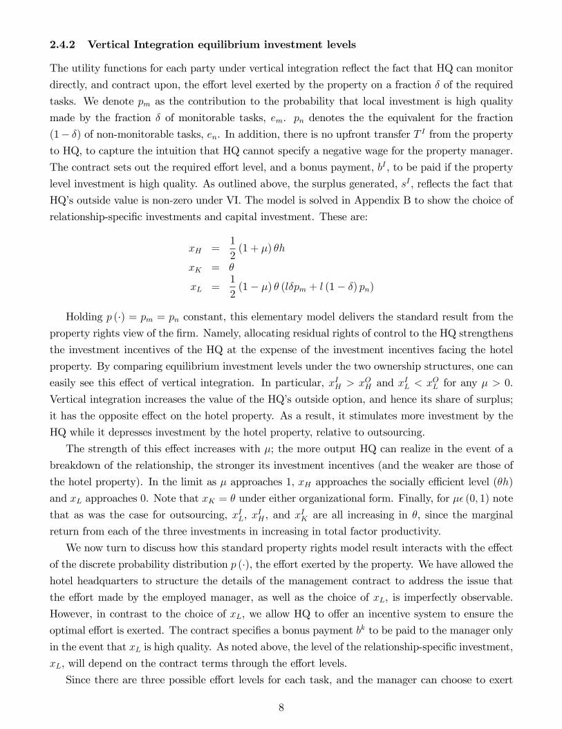
2.4.2 Vertical Integration equilibrium investment levels

The utility functions for each party under vertical integration re�ect the fact that HQ can monitor

directly, and contract upon, the e¤ort level exerted by the property on a fraction � of the required

tasks. We denote pm as the contribution to the probability that local investment is high quality

made by the fraction � of monitorable tasks, em. pn denotes the the equivalent for the fraction

(1� �) of non-monitorable tasks, en. In addition, there is no upfront transfer T I from the propertyto HQ, to capture the intuition that HQ cannot specify a negative wage for the property manager.

The contract sets out the required e¤ort level, and a bonus payment, bI , to be paid if the property

level investment is high quality. As outlined above, the surplus generated, sI , re�ects the fact that

HQ�s outside value is non-zero under VI. The model is solved in Appendix B to show the choice of

relationship-speci�c investments and capital investment. These are:

xH =1

2(1 + �) �h

xK = �

xL =1

2(1� �) � (l�pm + l (1� �) pn)

Holding p (�) = pm = pn constant, this elementary model delivers the standard result from the

property rights view of the �rm. Namely, allocating residual rights of control to the HQ strengthens

the investment incentives of the HQ at the expense of the investment incentives facing the hotel

property. By comparing equilibrium investment levels under the two ownership structures, one can

easily see this e¤ect of vertical integration. In particular, xIH > xOH and xIL < xOL for any � > 0.

Vertical integration increases the value of the HQ�s outside option, and hence its share of surplus;

it has the opposite e¤ect on the hotel property. As a result, it stimulates more investment by the

HQ while it depresses investment by the hotel property, relative to outsourcing.

The strength of this e¤ect increases with �; the more output HQ can realize in the event of a

breakdown of the relationship, the stronger its investment incentives (and the weaker are those of

the hotel property). In the limit as � approaches 1, xH approaches the socially e¢ cient level (�h)

and xL approaches 0. Note that xK = � under either organizational form. Finally, for �� (0; 1) note

that as was the case for outsourcing, xIL, xIH , and x

IK are all increasing in �, since the marginal

return from each of the three investments in increasing in total factor productivity.

We now turn to discuss how this standard property rights model result interacts with the e¤ect

of the discrete probability distribution p (�), the e¤ort exerted by the property. We have allowed thehotel headquarters to structure the details of the management contract to address the issue that

the e¤ort made by the employed manager, as well as the choice of xL, is imperfectly observable.

However, in contrast to the choice of xL, we allow HQ to o¤er an incentive system to ensure the

optimal e¤ort is exerted. The contract speci�es a bonus payment bk to be paid to the manager only

in the event that xL is high quality. As noted above, the level of the relationship-speci�c investment,

xL, will depend on the contract terms through the e¤ort levels.

Since there are three possible e¤ort levels for each task, and the manager can choose to exert

8

a di¤erent amount of e¤ort on the groups of non-monitored tasks to that which he is contracted

to exert on monitored tasks, there are nine possible combinations of overall e¤ort level that can be

exerted. In each case, the bonus payment must ensure that the manager�s expected payo¤ satis�es

his participation and the equilibrium e¤ort levels satisfy his incentive compatibility constraints.

The payo¤s to HQ in each of the nine possible scenarios are derived in Appendix B.

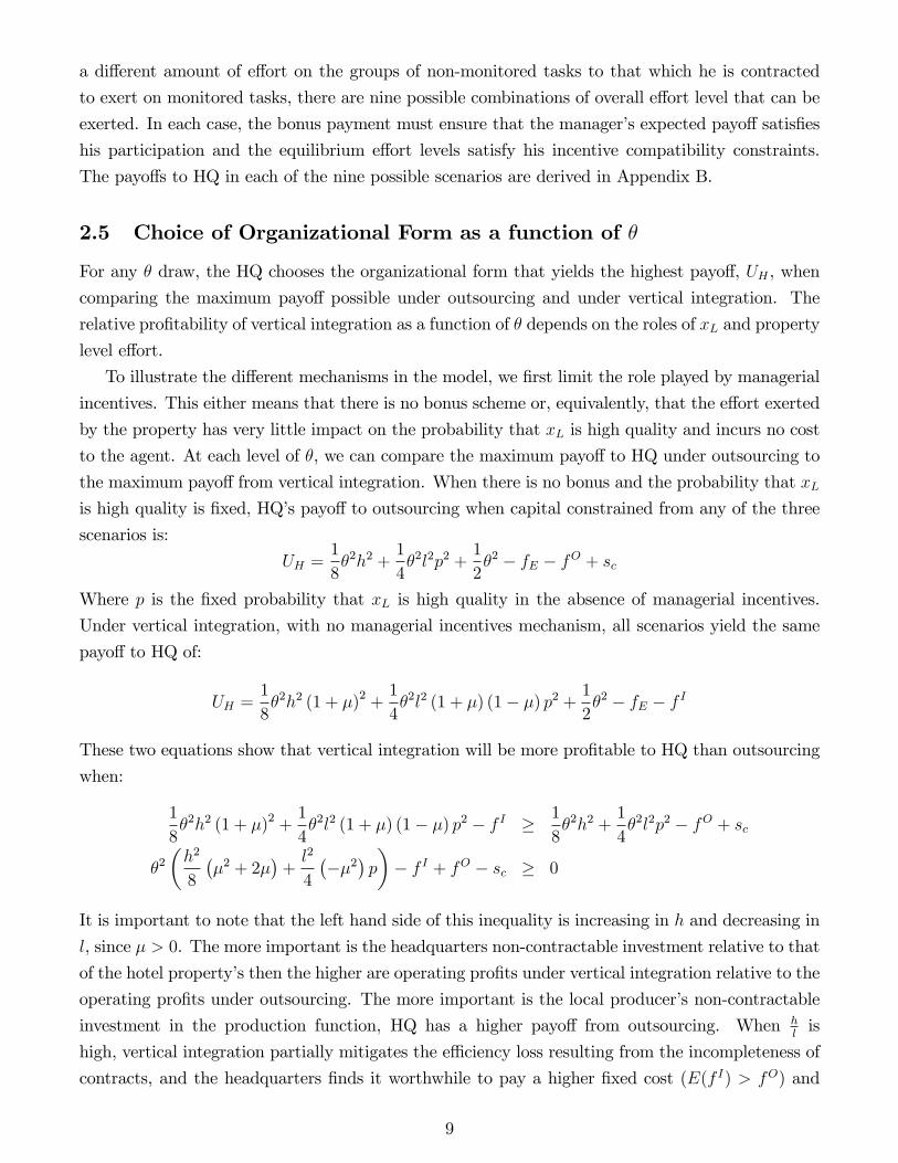
2.5 Choice of Organizational Form as a function of �

For any � draw, the HQ chooses the organizational form that yields the highest payo¤, UH , when

comparing the maximum payo¤ possible under outsourcing and under vertical integration. The

relative pro�tability of vertical integration as a function of � depends on the roles of xL and property

level e¤ort.

To illustrate the di¤erent mechanisms in the model, we �rst limit the role played by managerial

incentives. This either means that there is no bonus scheme or, equivalently, that the e¤ort exerted

by the property has very little impact on the probability that xL is high quality and incurs no cost

to the agent. At each level of �, we can compare the maximum payo¤ to HQ under outsourcing to

the maximum payo¤ from vertical integration. When there is no bonus and the probability that xLis high quality is �xed, HQ�s payo¤ to outsourcing when capital constrained from any of the three

scenarios is:

UH =1

8�2h2 +

1

4�2l2p2 +

1

2�2 � fE � fO + sc

Where p is the �xed probability that xL is high quality in the absence of managerial incentives.

Under vertical integration, with no managerial incentives mechanism, all scenarios yield the same

payo¤ to HQ of:

UH =1

8�2h2 (1 + �)2 +

1

4�2l2 (1 + �) (1� �) p2 + 1

2�2 � fE � f I

These two equations show that vertical integration will be more pro�table to HQ than outsourcing

when:

1

8�2h2 (1 + �)2 +

1

4�2l2 (1 + �) (1� �) p2 � f I � 1

8�2h2 +

1

4�2l2p2 � fO + sc

�2�h2

8

��2 + 2�

�+l2

4

���2

�p

�� f I + fO � sc � 0

It is important to note that the left hand side of this inequality is increasing in h and decreasing in

l, since � > 0. The more important is the headquarters non-contractable investment relative to that

of the hotel property�s then the higher are operating pro�ts under vertical integration relative to the

operating pro�ts under outsourcing. The more important is the local producer�s non-contractable

investment in the production function, HQ has a higher payo¤ from outsourcing. When hlis

high, vertical integration partially mitigates the e¢ ciency loss resulting from the incompleteness of

contracts, and the headquarters �nds it worthwhile to pay a higher �xed cost (E(f I) > fO) and

9

give up the transfer payment equivalent to sc to organize production in this way.

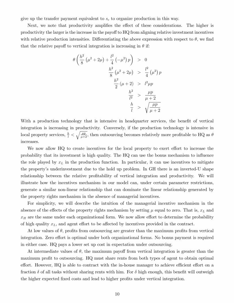
Next, we note that productivity ampli�es the e¤ect of these considerations. The higher is

productivity the larger is the increase in the payo¤to HQ from aligning relative investment incentives

with relative production intensities. Di¤erentiating the above expression with respect to �, we �nd

that the relative payo¤ to vertical integration is increasing in � if:

�

�h2

8

��2 + 2�

�+l2

4

���2

�p

�> 0

h2

8

��2 + 2�

�>

l2

4

��2�p

h2

2(�+ 2) > l2�p

h2

l2>

�p

�+ 2

h

l>

r�p

�+ 2

With a production technology that is intensive in headquarter services, the bene�t of vertical

integration is increasing in productivity. Conversely, if the production technology is intensive in

local property services, hl<q

�p�+2, then outsourcing becomes relatively more pro�table to HQ as �

increases.

We now allow HQ to create incentives for the local property to exert e¤ort to increase the

probability that its investment is high quality. The HQ can use the bonus mechanism to in�uence

the role played by xL in the production function. In particular, it can use incentives to mitigate

the property�s underinvestment due to the hold up problem. In GH there is an inverted-U shape

relationship between the relative pro�tability of vertical integration and productivity. We will

illustrate how the incentives mechanism in our model can, under certain parameter restrictions,

generate a similar non-linear relationship that can dominate the linear relationship generated by

the property rights mechanism in the absence of managerial incentives.

For simplicity, we will describe the intuition of the managerial incentive mechanism in the

absence of the e¤ects of the property rights mechanism by setting � equal to zero. That is, xL and

xH are the same under each organizational form. We now allow e¤ort to determine the probability

of high quality xL, and agent e¤ort to be a¤ected by incentives provided in the contract.

At low values of �, pro�ts from outsourcing are greater than the maximum pro�ts from vertical

integration. Zero e¤ort is optimal under both organizational forms. No bonus payment is required

in either case. HQ pays a lower set up cost in expectation under outsourcing.

At intermediate values of �, the maximum payo¤ from vertical integration is greater than the

maximum pro�t to outsourcing. HQ must share rents from both types of agent to obtain optimal

e¤ort. However, HQ is able to contract with the in-house manager to achieve e¢ cient e¤ort on a

fraction � of all tasks without sharing rents with him. For � high enough, this bene�t will outweigh

the higher expected �xed costs and lead to higher pro�ts under vertical integration.

10

At high levels of �, the optimal outsourcing contract involves maximum e¤ort on all tasks. As

� increases, the HQ has more to gain, even if it pays a bonus, from ensuring e = E is exerted

on even the share of tasks that are not directly monitorable under vertical integration. Thus the

relative advantage of being able to monitor the e¤ort exerted on a fraction of tasks under vertical

integration disappears. In addition, under outsourcing, HQ is able to extract some up front fee from

the agent, sc, and incur lower set up costs. These considerations mean that the maximum pro�ts

to HQ under outsourcing are greater than under vertical integration at high levels of �.

In Appendix C, we present four di¤erent examples to illustrate outcomes of the model under

di¤erent parameter values of the relationship between productivity, �, and the relative pro�tability

of vertical integration and outsourcing.

2.6 Testable Implications

The four cases outline above demonstrate di¤erent scenarios for possible relationship between �

and the relative pro�tability of vertical integration and outsourcing. The greater the di¤erence in

predicted pro�tability between organizational form, the larger would have to be the stochastic term

speci�c to the particular relationship to overturn the prediction that HQ will select the organiza-

tional form predicted to generate the highest payo¤ to HQ. This tells us that the probability that

the HQ will vertically integrate depends on the extent to which the maximum expected payo¤ to

vertical integration as a function of � outweighs the maximum expected payo¤ at that � draw to

outsourcing. The model hence generates (at least) two related predictions.

1. For a production technology either intensive in HQ or property level services, where manage-

rial incentives plays no role in in�uencing the choice of organizational form and relationship-

speci�c investments are determined by the possibility of hold up in the event of failed bar-

gaining, the probability of vertical integration either increases or decreases with productivity.

There is a monotonic predicted relationship between � and the relative pro�tability of vertical

integration.

2. For a production technology where HQ is able to o¤er a contract which a¤ects property-

level e¤ort and the quality of the property�s relationship-speci�c investment, there will be

a non-linear relationship between the probability of vertical integration and productivity.

Outsourcing will be relatively more pro�table to HQ for high and low levels of productivity,

�, and vertical integration is relatively more pro�table for intermediate levels of productivity.

Since property-level total factor productivity data are not available to use a present, we test

these propositions indirectly by examining the predicted relationship between the probability of

integration and the level of capital investment. In particular, we exploit the fact that the model

generates a third prediction:

3. xk increases with �.

11

Hence, the model implies that variations in productivity induce a relationship between xk and

the probability of vertical integration that is similar to the underlying relationship between � and

organizational form. In the second part of the paper, we directly test these predicted relationships:

1. For a production technology where property rights concerns determine the choice of organiza-

tional form in the absence of e¤ective managerial incentives, there is a monotonic relationship

between the probability of integration and the level of capital investment.

2. For a production technology where managerial incentives play a signi�cant role in in�uencing

the quality of the property-level input (or relationship speci�c investment level), there is

a non-monotonic relationship between the probability of integration and the level of capital

investment. In particular, there is an inverted-U shaped relationship between the two variables

such that medium sized hotels are more likely to be vertically integrated.

3 Description of Data

To test the predictions of the model, we employ property-level data from two hotel �rms and from

one market research �rm. The primary data include 11 brands and their 1168 hotels worldwide.

The secondary data include 9 additional brands and their 2970 hotels in the US. For each hotel

property in the dataset, we have data on location (city and country), the number of rooms, and

organizational form. In addition, the secondary data also include the opening date of each hotel

and the date that the hotel �rst became a¢ liated with its current brand. Table 4 summarizes the

available information in the primary and secondary data.

Organizational form is a categorical variable, with the categories in the primary data di¤ering

from the categories in the secondary data. In the primary data, there is information on two related

but distinct dimensions of integration: whether the headquarters owns a hotel property and whether

the headquarters operates or manages a hotel property. As a result, there are four main categories

of hotels: owned, leased, managed, and franchised. For an owned or franchised property, one party

owns and operates the property. For an owned property, that party is the headquarters; for a

franchised property, it is a third party. For a leased property, the headquarters owns the property

and leases it to a third party who operates it. Finally, for a managed property, a third party owns

the property but the headquarters manages it. In the secondary data, there is information on

operation but not on ownership. As a result, there are only two categories of organizational form:

franchised and chain management.

Based on these categories, we create three alternative measures of vertical integration. First,

the binary variable VI indicates whether either ownership or operation of the hotel property is

outsourced to a third party. It is equal to 1 if neither task is outsourced. Second, the binary

variable HQOWND indicates whether or not the headquarters owns a hotel property. Third, the

binary variable HQOPED is an indicator for whether not the headquarters operates a hotel property.

Figure 1 summarizes the mapping from the categorical variables in the raw data to the binary

12

variables HQOWND and HQOPED. Hotels with a value of 1 for VI are in the top right hand

box of the �gure. In the secondary data there are only two categories, the two grey-shaded values:

"chain management" and "franchised." "Franchised" corresponds to a value of 0 for both HQOPED

and HQOWND. "Chain management" corresponds to a value of 1 for HQOPED; the value of

HQOWND is unknown in this case. In the primary data, there are �ve categories: managed, rented,

owned, leased, and franchised. All of these values are informative about both asset ownership and

organizational control; accordingly, each one maps to HQOPED and HQOWND as shown in Figure

1.

There is an average propensity towards outsourcing in the relevant data for each of the three

measure. In the primary data, only 17% of hotels are entirely vertically integrated, where both

ownership and operation of the hotel property are done in house. Also based on the primary data,

18% of the hotels are owned by the headquarters. In the complete data set, 31% of the hotels

are operated by the headquarters. Table 5 presents summary statistics for hotel size, integration,

opening date, and a¢ liation date for various subsets of the data.

Figures 2 and 3 present some graphical evidence that variation in organizational form may be

associated with hotel size in a manner consistent with the theories. For three di¤erent brands,

Figure 2 shows the proportion of US hotels in each hotel size bin that is owned by HQ. Brands B

and C6 provide some evidence of an inverted-U shaped relationship. For Brand C, there appears to

be a positive correlation of the type predicted by the property rights model (for large hl). Figure 3

shows the same data for �ve brands which, on average, have fewer rooms per hotel. Here, we see

evidence of an inverted-U shape for Brand B, HOLS (Holiday Inn & Suites) and RADI (Radisson).

The pattern for the other brands is less clear. These �gures suggest that some of the predicted

relationships may obtain in the data. We now turn to a more formal test of those propositions.

4 Estimation Strategy

Our dependent variables are binary; vertical integration corresponds to 1 and outsourcing corre-

sponds to 0. We have two alternative dependent variables: HQOWND, and HQOPED. In each

case, the outcome of these discrete choices can be seen as re�ecting a threshold rule for an under-

lying latent variable y� (Greene, 2002), so that y = 1 if y� > 0 and y = 0 if y� � 0. In this

case, the vector of latent variables y� is the di¤erence between pro�ts under vertical integration

and outsourcing. We can write a threshold rule based on the realization of the pro�t di¤erential

between the two organizational forms. At di¤erent levels of �, the stochastic elements of the model

are di¤erently likely to overturn the prediction that HQ will choose the organizational form that

yields the highest UH , so that if predicted y� is positive, vertical integration will be chosen and if

y� is negative, outsourcing will be chosen.

Since we do not directly observe the pro�t di¤erential y� we use the outcome of vertical inte-

6We obtained primary data directly from two multinational hotel �rms under a strict con�dentiality agreement.Accordingly, we disguise the brand names using letter codes.

13

gration or outsourcing to infer the parameters in the underlying model. We assume that y� is a

function of the set of explanatory variables generated by the model, x; we use the linear approx-imation y� = �0x + ". We normalize variables so that " has a standard logistic distribution with

mean zero and variance one.

We include group e¤ects among these explanatory variables in order to mitigate omitted vari-

able bias. The model implies that brand and market characteristics other than productivity may

a¤ect both hotel size and organizational form. For example, for an HQ-intensive technology, a

higher �xed cost of entry for a particular brand-country pair will increase average hotel size and

the average probability of vertical integration. Because we cannot directly measure some of these

characteristics, we group e¤ects among our explanatory variables x. E¤ectively, this allows the pro-

ductivity distribution, F (�), and other inputs to the various pro�t functions to vary by group. This

speci�cation sweeps out the e¤ects that are common to all observations in each group; identi�cation

comes from the within-group variation in the dependent variables. Given these assumptions, the

probability that the l�th hotel of the n�th group will be integrated (ynl = 1) can be rewritten as:

Pr (y�nl > 0jxnl;�) = Pr (�0exnl + �n + "nl > 0) = F (�0exnl + �n) (4)

where �n is a group speci�c incidental parameter common to all other observations in group n andexnl consists of the other regressors speci�c to hotel l in group n.In our baseline estimates, we use brand-country groups. In order to control for a wide range of

group e¤ects, we allow the brand e¤ect to di¤er across countries and vice versa. We also perform

a robustness check in which we use city and brand group e¤ects, in order to control for omitted

variables at the sub-country level that may be correlated with size and organizational form.7 In both

cases, the average group size is not large and there are a number of very small groups. For each of

the three measures of vertical integration, Table 3 presents the size of the groups used in our baseline

estimates and our check for robustness to controls for potential city-level omitted variables. With

HQOWND and brand-country groups, the average group size is 20, but there are groups with as few

as 2 observations. These small groups complicate our estimation strategy. Conventional maximum

likelihood estimation of a non-linear probability model with �xed e¤ects will yield inconsistent

parameter estimates, and the problem is particularly severe in the case of many groups with few

observations per group. This point is illustrated in Chamberlain (1980). Since the bias of the

�xed e¤ect estimates is typically on the order of 1Ln, where Ln is the number of observations in

the n�th group, the potential for bias is signi�cant. Accordingly, we adopt the remedy suggested

in Chamberlain (1980) and employ a conditional likelihood approach.8 In addition, because we

7A third speci�cation using brand-city groups is discussed in Appendix D. We do not have enough within groupvariation to identify brand level e¤ects, but our results remain for the pooled sample.

8 The estimator of � generated from the conditional logit maximum likelihood estimation is consistent as long asthe conditional likelihood function satis�es regularity conditions (Chamberlain, 1980). The asymptotic covariancematrix for the estimator of � is obtained from the inverse of the information matrix, allowing us to use standarderror estimates to make inferences about the e¤ects of the each of the explanatory variables in ex on the choice oforganizational form, yn;l.

14

explicitly include brand �xed e¤ects in our speci�cation with city and brand group e¤ects9, we

exclude observations for brands with fewer than 47 observations10. Table 2 indicates that this

latter step excludes only 72 out of 4138 observations.

Rewriting the problem in panel form to illustrate group a¢ liation, let n = 1::::N index the

group, and let l = 1:::Ln index the observations in group n. We condition the likelihood function

on the number of positive outcomes in each group n, which is a summary statistic for the group-

speci�c incidental parameter. Let yn = (yn;1; yn;2; :::yn;Ln) be the series of observed outcomes for

the n�th group as a whole. We denote the observed number of ones for the dependent variable in

the n�th group as kn =PLn

l=1 yn;l. We are interested in the probability of a possible set of outcomes

yn conditional on the observed value of kn. The conditional likelihood function can be written:

L = �n Pr

ynj

LnXl=1

yn;l = kn

!(5)

and is independent of �n; the incidental parameters have been swept out of the likelihood function.

In the context of a logit model, the conditional probability of observing the series of outcomes ynin group n, conditional on kn is expressed:

Pr

ynj

LnXl=1

yn;l = kn

!=

exp�PLn

l=1 yn;lexn;l��Pdn�Sn

exp�PLn

l=1 dn;lexn;l�� (6)

where dn;l is equal to 0 or 1 withPLn

l=1 dn;l = kn, and Sn is the set of all possible combinations of

kn ones and (Ln � kn) zeros11.We allow the parameters � to di¤er across brands in our baseline estimation. Our hypothesis

is that the most important determinants of organizational form vary across brands, so that each

theory may better predict outcomes for some brands than it does for others. Using this framework,

we estimate reduced form quadratic models of the latent variable y�cbl of the following type:

y�cbl = �cb + �11ROOMScbl +BXz=2

[I(z = b)] �1zROOMScbl

+�21 (ROOMScbl)2 +

BXz=2

[I(z = b)] �2z (ROOMScbl)2 + �cbl (7)

where I(z = b) is an indicator variable that takes on the value 1 if z = b and the value 0 otherwise,

ROOMScbl is the number of rooms for the l�th hotel of the country c -brand b group n, and �cb is

the group e¤ect for the country c-brand b pair.

9Since the average number of observations per brand is signi�cantly greater than the number of observations percity, we choose to condition on the number of positive outcomes per city.10In order to minimize di¤erences due to sample selection, we drop small brands in both the baseline estimates

and the robustness checks.11This formulation of the summary notation is taken from Hosmer and Lemeshow (2000), equation 7.4.

15

To test whether the property rights e¤ect in the model dominates the choice of organizational

form, we estimate this model and then test the following restriction on the estimated coe¢ cients:

for any given brand, @y�

@ROOMShas the same sign for all values of ROOMS. To test whether the

managerial incentives e¤ect plays a signi�cant role in determining organizational form, we test the

following two restrictions on the coe¢ cient estimates. First, the estimated coe¢ cient on ROOMS

should be positive and the estimated coe¢ cient on ROOMS2 should be negative. Second, these

coe¢ cients should be such that @y�

@ROOMS> 0 for low values of ROOMS and @y�

@ROOMS< 0 for higher

values of ROOMS.

5 Empirical results

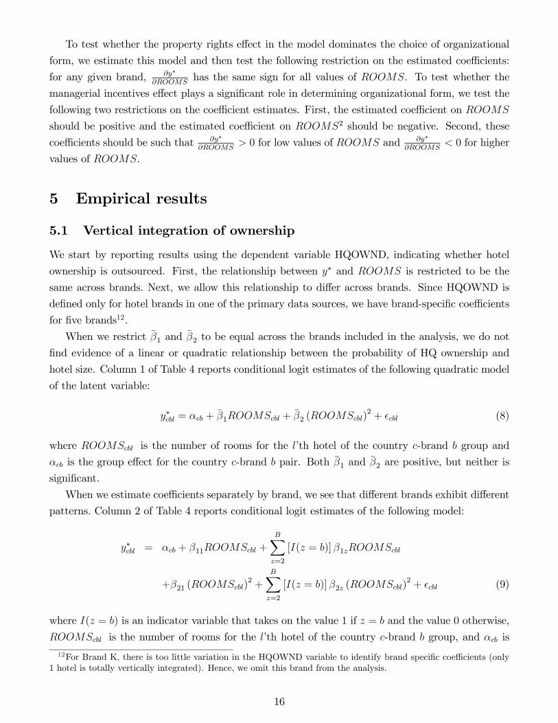
5.1 Vertical integration of ownership

We start by reporting results using the dependent variable HQOWND, indicating whether hotel

ownership is outsourced. First, the relationship between y� and ROOMS is restricted to be the

same across brands. Next, we allow this relationship to di¤er across brands. Since HQOWND is

de�ned only for hotel brands in one of the primary data sources, we have brand-speci�c coe¢ cients

for �ve brands12.

When we restrict ��1 and ��2 to be equal across the brands included in the analysis, we do not

�nd evidence of a linear or quadratic relationship between the probability of HQ ownership and

hotel size. Column 1 of Table 4 reports conditional logit estimates of the following quadratic model

of the latent variable:

y�cbl = �cb +��1ROOMScbl + ��2 (ROOMScbl)

2 + �cbl (8)

where ROOMScbl is the number of rooms for the l�th hotel of the country c-brand b group and

�cb is the group e¤ect for the country c-brand b pair. Both ��1 and ��2 are positive, but neither is

signi�cant.

When we estimate coe¢ cients separately by brand, we see that di¤erent brands exhibit di¤erent

patterns. Column 2 of Table 4 reports conditional logit estimates of the following model:

y�cbl = �cb + �11ROOMScbl +

BXz=2

[I(z = b)] �1zROOMScbl

+�21 (ROOMScbl)2 +

BXz=2

[I(z = b)] �2z (ROOMScbl)2 + �cbl (9)

where I(z = b) is an indicator variable that takes on the value 1 if z = b and the value 0 otherwise,

ROOMScbl is the number of rooms for the l�th hotel of the country c-brand b group, and �cb is

12For Brand K, there is too little variation in the HQOWND variable to identify brand speci�c coe¢ cients (only1 hotel is totally vertically integrated). Hence, we omit this brand from the analysis.

16

the group e¤ect for the country c-brand b pair. It is clear from this table that there are important

di¤erences between brands.

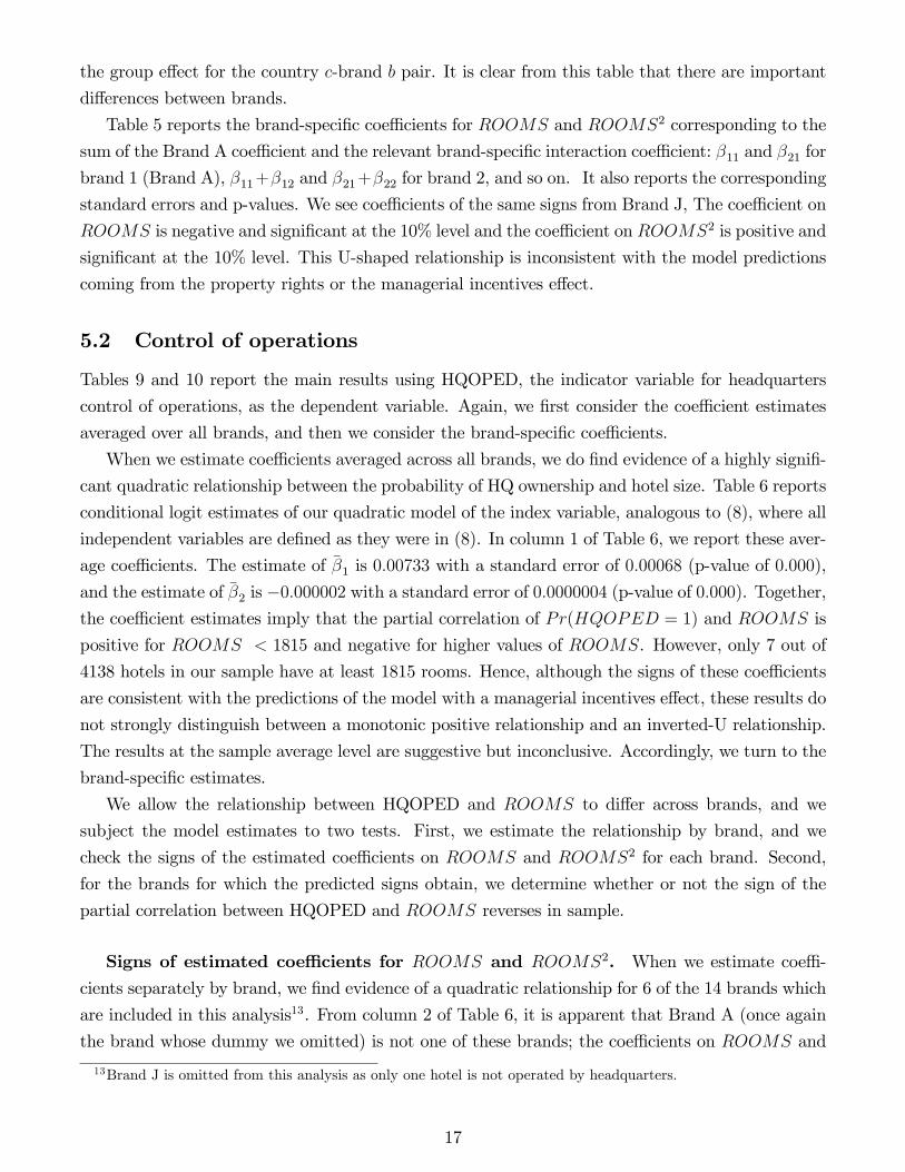
Table 5 reports the brand-speci�c coe¢ cients for ROOMS and ROOMS2 corresponding to the

sum of the Brand A coe¢ cient and the relevant brand-speci�c interaction coe¢ cient: �11 and �21 for

brand 1 (Brand A), �11+�12 and �21+�22 for brand 2, and so on. It also reports the corresponding

standard errors and p-values. We see coe¢ cients of the same signs from Brand J, The coe¢ cient on

ROOMS is negative and signi�cant at the 10% level and the coe¢ cient on ROOMS2 is positive and

signi�cant at the 10% level. This U-shaped relationship is inconsistent with the model predictions

coming from the property rights or the managerial incentives e¤ect.

5.2 Control of operations

Tables 9 and 10 report the main results using HQOPED, the indicator variable for headquarters

control of operations, as the dependent variable. Again, we �rst consider the coe¢ cient estimates

averaged over all brands, and then we consider the brand-speci�c coe¢ cients.

When we estimate coe¢ cients averaged across all brands, we do �nd evidence of a highly signi�-

cant quadratic relationship between the probability of HQ ownership and hotel size. Table 6 reports

conditional logit estimates of our quadratic model of the index variable, analogous to (8), where all

independent variables are de�ned as they were in (8). In column 1 of Table 6, we report these aver-

age coe¢ cients. The estimate of ��1 is 0:00733 with a standard error of 0:00068 (p-value of 0:000),

and the estimate of ��2 is �0:000002 with a standard error of 0:0000004 (p-value of 0:000). Together,the coe¢ cient estimates imply that the partial correlation of Pr(HQOPED = 1) and ROOMS is

positive for ROOMS < 1815 and negative for higher values of ROOMS. However, only 7 out of

4138 hotels in our sample have at least 1815 rooms. Hence, although the signs of these coe¢ cients

are consistent with the predictions of the model with a managerial incentives e¤ect, these results do

not strongly distinguish between a monotonic positive relationship and an inverted-U relationship.

The results at the sample average level are suggestive but inconclusive. Accordingly, we turn to the

brand-speci�c estimates.

We allow the relationship between HQOPED and ROOMS to di¤er across brands, and we

subject the model estimates to two tests. First, we estimate the relationship by brand, and we

check the signs of the estimated coe¢ cients on ROOMS and ROOMS2 for each brand. Second,

for the brands for which the predicted signs obtain, we determine whether or not the sign of the

partial correlation between HQOPED and ROOMS reverses in sample.

Signs of estimated coe¢ cients for ROOMS and ROOMS2. When we estimate coe¢ -

cients separately by brand, we �nd evidence of a quadratic relationship for 6 of the 14 brands which

are included in this analysis13. From column 2 of Table 6, it is apparent that Brand A (once again

the brand whose dummy we omitted) is not one of these brands; the coe¢ cients on ROOMS and

13Brand J is omitted from this analysis as only one hotel is not operated by headquarters.

17

ROOMS2 are both positive but insigni�cant. Table 7 reports brand-speci�c coe¢ cients for the

remaining brands (obtained by summing coe¢ cients as before) and the corresponding standard

errors and p-values. For Brand B, Hampton Inn, Hilton, Holiday Inn, Radisson, and Brand C

(BR_B, HAMI, HILU, HOLI, RADI, BR_C), the coe¢ cient on ROOMS is positive and signi�-

cant at 5 percent, and the coe¢ cient on ROOMS2 is negative and signi�cant at 5 percent, which is

consistent with a managerial incentives e¤ect. For Marriott, the coe¢ cient on ROOMS is 0:0062

and signi�cant at 1 percent and, while the coe¢ cient on ROOMS2 is negative as predicted by the

managerial incentives theory, it is insigni�cant. This pattern could be reconciled with either of the

two mechanisms. For the remaining 7 brands, none of the coe¢ cient estimates are signi�cant.

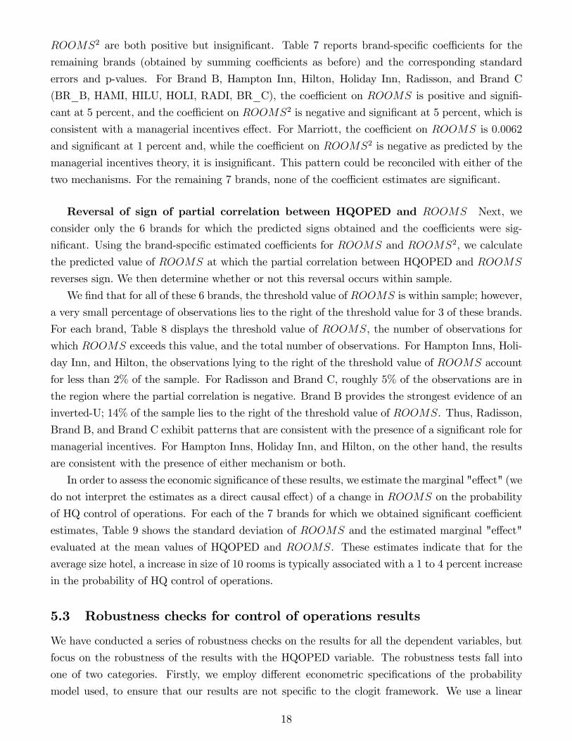
Reversal of sign of partial correlation between HQOPED and ROOMS Next, we

consider only the 6 brands for which the predicted signs obtained and the coe¢ cients were sig-

ni�cant. Using the brand-speci�c estimated coe¢ cients for ROOMS and ROOMS2, we calculate

the predicted value of ROOMS at which the partial correlation between HQOPED and ROOMS

reverses sign. We then determine whether or not this reversal occurs within sample.

We �nd that for all of these 6 brands, the threshold value of ROOMS is within sample; however,

a very small percentage of observations lies to the right of the threshold value for 3 of these brands.

For each brand, Table 8 displays the threshold value of ROOMS, the number of observations for

which ROOMS exceeds this value, and the total number of observations. For Hampton Inns, Holi-

day Inn, and Hilton, the observations lying to the right of the threshold value of ROOMS account

for less than 2% of the sample. For Radisson and Brand C, roughly 5% of the observations are in

the region where the partial correlation is negative. Brand B provides the strongest evidence of an

inverted-U; 14% of the sample lies to the right of the threshold value of ROOMS. Thus, Radisson,

Brand B, and Brand C exhibit patterns that are consistent with the presence of a signi�cant role for

managerial incentives. For Hampton Inns, Holiday Inn, and Hilton, on the other hand, the results

are consistent with the presence of either mechanism or both.

In order to assess the economic signi�cance of these results, we estimate the marginal "e¤ect" (we

do not interpret the estimates as a direct causal e¤ect) of a change in ROOMS on the probability

of HQ control of operations. For each of the 7 brands for which we obtained signi�cant coe¢ cient

estimates, Table 9 shows the standard deviation of ROOMS and the estimated marginal "e¤ect"

evaluated at the mean values of HQOPED and ROOMS. These estimates indicate that for the

average size hotel, a increase in size of 10 rooms is typically associated with a 1 to 4 percent increase

in the probability of HQ control of operations.

5.3 Robustness checks for control of operations results

We have conducted a series of robustness checks on the results for all the dependent variables, but

focus on the robustness of the results with the HQOPED variable. The robustness tests fall into

one of two categories. Firstly, we employ di¤erent econometric speci�cations of the probability

model used, to ensure that our results are not speci�c to the clogit framework. We use a linear

18

probability model and a logit model with brand �xed e¤ects14. Secondly, we address the concern

that our speci�cation omits variables that in�uence both organizational form and hotel size. We

include controls for the age of the hotel and the length of a¢ liation with its current brand. We

then ensure that our baseline results are not due to city speci�c incidental parameters by redoing

the baseline analysis using clogit and grouping at the city level, rather than at the country level.

We also cluster the observations at the city level to allow for non-independence of error terms for

observations drawn from the same city. Appendix D gives a description of the various robustness

checks and the results. We �nd that our key �ndings are robust to econometric speci�cation and,

for the most part, to controlling for potential omitted variables.15

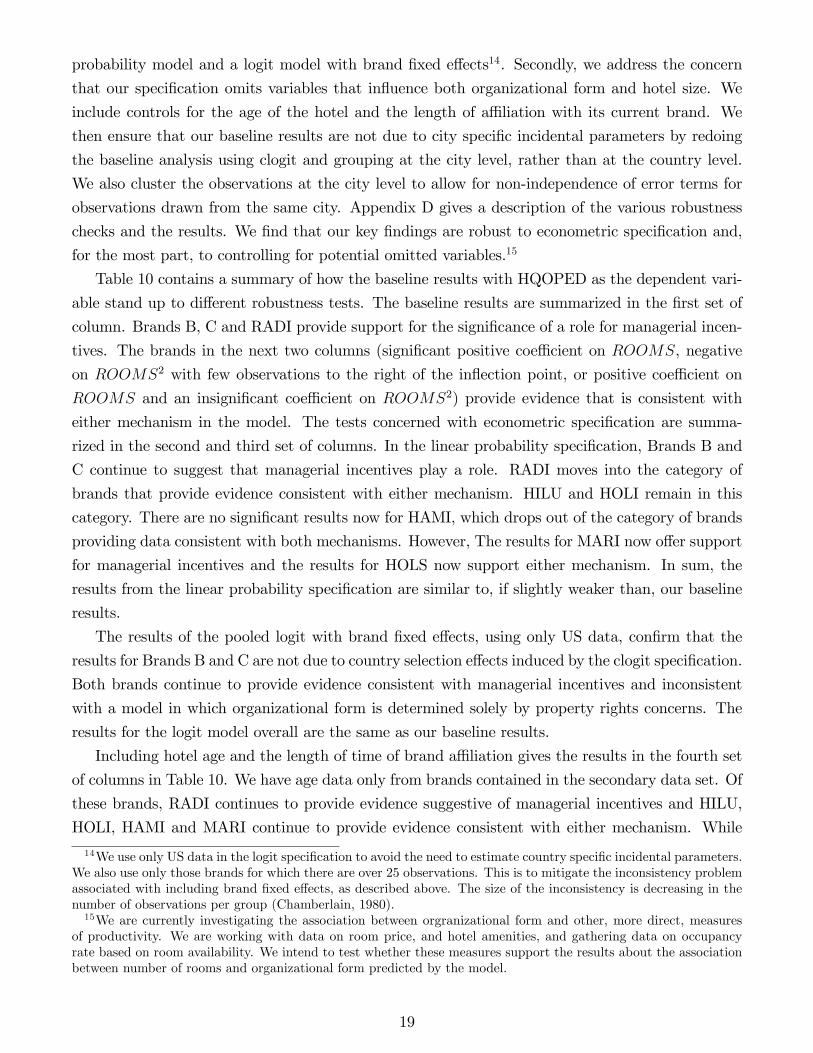
Table 10 contains a summary of how the baseline results with HQOPED as the dependent vari-

able stand up to di¤erent robustness tests. The baseline results are summarized in the �rst set of

column. Brands B, C and RADI provide support for the signi�cance of a role for managerial incen-

tives. The brands in the next two columns (signi�cant positive coe¢ cient on ROOMS, negative

on ROOMS2 with few observations to the right of the in�ection point, or positive coe¢ cient on

ROOMS and an insigni�cant coe¢ cient on ROOMS2) provide evidence that is consistent with

either mechanism in the model. The tests concerned with econometric speci�cation are summa-

rized in the second and third set of columns. In the linear probability speci�cation, Brands B and

C continue to suggest that managerial incentives play a role. RADI moves into the category of

brands that provide evidence consistent with either mechanism. HILU and HOLI remain in this

category. There are no signi�cant results now for HAMI, which drops out of the category of brands

providing data consistent with both mechanisms. However, The results for MARI now o¤er support

for managerial incentives and the results for HOLS now support either mechanism. In sum, the

results from the linear probability speci�cation are similar to, if slightly weaker than, our baseline

results.

The results of the pooled logit with brand �xed e¤ects, using only US data, con�rm that the

results for Brands B and C are not due to country selection e¤ects induced by the clogit speci�cation.

Both brands continue to provide evidence consistent with managerial incentives and inconsistent

with a model in which organizational form is determined solely by property rights concerns. The

results for the logit model overall are the same as our baseline results.

Including hotel age and the length of time of brand a¢ liation gives the results in the fourth set

of columns in Table 10. We have age data only from brands contained in the secondary data set. Of

these brands, RADI continues to provide evidence suggestive of managerial incentives and HILU,

HOLI, HAMI and MARI continue to provide evidence consistent with either mechanism. While

14We use only US data in the logit speci�cation to avoid the need to estimate country speci�c incidental parameters.We also use only those brands for which there are over 25 observations. This is to mitigate the inconsistency problemassociated with including brand �xed e¤ects, as described above. The size of the inconsistency is decreasing in thenumber of observations per group (Chamberlain, 1980).15We are currently investigating the association between orgranizational form and other, more direct, measures

of productivity. We are working with data on room price, and hotel amenities, and gathering data on occupancyrate based on room availability. We intend to test whether these measures support the results about the associationbetween number of rooms and organizational form predicted by the model.

19

the age variables are related to hotel size, their inclusion does not signi�cantly alter the baseline

results.

The last two sets of columns contain the results from two di¤erent ways of controlling for omitted

city-level variables. In the �fth column, we estimate a clogit model with city groups and brand �xed

e¤ects. Of the three brands that supported the role of managerial incentives in the baseline analysis,

two continue to do so (Brand C and RADI). The coe¢ cients for Brand B cease to be signi�cant.

Of the 4 brands that provided evidence consistent with both mechanisms, three continue to do so.

HILU actually moves from this category and now provides results consistent only with a model that

includes the managerial incentives mechanism, and a larger share of hotel properties are now to the

right of the in�ection point. The fact that the estimated coe¢ cients on Brand B lose signi�cance

could be attributable to two factors. One is that the baseline results are due to city level factors

for these brands, rather than the predicted relationship between size and organizational form -

for example, in a particular city all the hotels happen to be both large and, independently, of a

particular organizational form. The other possible reason is data selection. The coe¢ cients are now

identi�ed on the hotels for each brand that are in cities where there is at least one hotel of any

brand, and variation in organizational form. These results suggest that city level factors may be

important for Brand B, but that the baseline results for the other brands are robust to controlling

for city level factors.

The last column of results presents the �ndings from the US logit model with brand �xed e¤ects,

clustering the observations at the city level to allow for a common component to error terms for

observations from the same city. The results from this speci�cation are very similar to the baseline

�ndings. The only di¤erence is that HILU now provides evidence consistent only with a model

that includes managerial incentives. They suggest that for the US data, while there is a city level

component of the error term, the association between hotel size and organizational form found in

the baseline analysis is robust to the appropriate adjustments to the standard errors.

6 Conclusion

To the best of our knowledge, this paper is the �rst to use �rm level data on organizational form and

producer characteristics to confront the predictions of the Antras Helpman (2004) and Grossman

Helpman (2004) models of the multinational �rm. We �nd signi�cant within-brand correlations

between organizational form and hotel size. The results show that, for a subset of brands, man-

agerial incentives play a more signi�cant role in determining whether or not to outsource hotel

operations that do property rights. A further subset of brands provide evidence consistent with

either mechanism.

The results for hotel operations are largely robust to controls for potential omitted variables at

various geographical levels and to controls for hotel age. Moreover, they are economically signi�cant;

for the average size hotel belonging to one of the seven brands that are consistent with at least one

theory, an increase in hotel size of 10 rooms is associated with a roughly 1-4 percent increase in the

20

probability of integration.

The results present a new puzzle. Why do some brands o¤er support for the importance of

managerial incentives - suggesting that decision making is in�uenced by principal-agent type con-

cerns - while others do not? We have asked whether hotel brand property portfolios di¤er in ways

that may help explain this variation. While gravity type variables, such as distance from HQ and

common legal origin, a¤ect the overall propensity to outsource operations at a property level, we do

not �nd strong evidence that di¤erences in portfolio characteristics at the brand level correlate with

whether managerial incentives matter for organizational form decisions.16 Further work is needed

to address the puzzle of why some brands are consistent with this mechanism and others are not.17

We also plan to re-estimate our speci�cations using alternative correlates of productivity. We are

in the process of conducting a hedonic analysis to estimate hotel-speci�c measures of productivity,

controlling for observed characteristics of the hotel including hotel brand and level of amenities. In

this productivity measure would be contained all the factors that are unobservable in our data set,

but which are observed by HQ and third parties when deciding on organizational form.

Our study has also highlighted an important empirical regularity that could guide future em-

pirical and theoretical research: there is some independent variation between asset ownership and

operational control. Managerial incentives appear to matter for hotel operation, but we can �nd no

evidence that they play a role in ownership decisions. In addition, we do not �nd any evidence that

property rights plays a role in determining ownership in this industry context. In empirical work,

the choice of the measure of vertical integration is highly consequential. A theory of the �rm that

explains the behavior of one variable may very well have little or no explanatory power over the

other one. A theory that simultaneously determines these two distinct dimensions of organizational

form, as in Feenstra and Hanson (2004), is critical in increasing our understanding of the modern

multinational corporation.

16These results are available on request.17One interesting fact is that brands under common control tend to exhibit similar behavior; either all or none

of the brands reveal a role for managerial incentives. Although Brands A to D are now under common control,within one hotel group, this group was formed through merger of di¤erent chains. Brands B and C share a corporatehistory and managerial incentives appear to be at work within both of these brands. Brands A and D were managedseparately prior to 1998. The Radisson brand is not in the same group as any other brand in our data set. Neitherbrand from Firm 2 (Brands K and J) o¤ers support for the managerial incentives mechanism, and neither does eitherof the Hyatt brands. From this we infer that attention to managerial incentives for any one hotel brand is correlatedacross commonly managed brands.

21

References

[1] Acemoglu, D., P. Aghion, R. Gri¢ th, and F. Zilibotti (2003), "Vertical Integration and Tech-

nology: Theory and Evidence," manuscript.

[2] Antras, P. (2003), "Incomplete Contracts and the Product Cycle," mimeo, Harvard University.

[3] Antras, P. and E. Helpman (2004), "Global Sourcing," forthcoming in Journal of Political

Economy.

[4] Baker, G. and T. Hubbard (2002), "Make Versus Buy in Trucking: Asset Ownership, Job

Design, and Information," mimeo, Harvard University.

[5] Brainard, Y. (1997), "An Empirical Assessment of the Proximity-Concentration Trade-o¤ Be-

tween Multinational Sales and Trade", The American Economic Review, 87, 4, 520-544.

[6] Brickley, J. and R. Dark (1987), "The Choice of Organizational Form: The Case of Franchis-

ing," Journal of Financial Economics, June 1987

[7] Chamberlain, G. (1980), "Analysis of Covariance with Qualitative Data." The Review of Eco-

nomic Studies, 41, 1, 225-238.

[8] Feenstra, R. and G. Hanson (2004), "Ownership and Control in Outsourcing to China: Esti-

mating the Property-Rights Theory of the Firm," NBER Working Paper No. 10198.

[9] Greene, W.H. (2002), "Econometric Analysis", 5th Edition, Prentice Hall.

[10] Grossman, G. and E. Helpman (2004), "Managerial Incentives and the International Organi-

zation of Production," forthcoming in Journal of International Economics.

[11] Grossman, S. and O. Hart (1986), "The Costs and Bene�ts of Ownership: A Theory of Vertical

and Lateral Integration," Journal of Political Economy, 94, 691-719.]

[12] Hart, O. and J. Moore (1990), "Property Rights and the Nature of the Firm," Journal of

Political Economy, 98, 1119-1158.

[13] Holmstrom, B. and P. Milgrom (1991), "Multitask Principal-Agent Analyses: Incentive Con-

tracts, Asset Ownership, and Job Design," Journal of Law, Economics and Organization 7,

24-52.

[14] Horn, H., Lang, H., and S. Lundgren (1995), "Managerial E¤ort, Incentives, X-ine¢ ciency and

International Trade," European Economic Review, 39, 117-138.

[15] Hosmer, D. and S. Lemeshow (2000), "Applied Logistic Regression", 2nd Edition, John Wiley

& Sons, New York.

22

[16] Klein, B., Crawford, R., and A. Alchian (1978), "Vertical Integration, Appropriable Rents, and

the Competitive Contracting Process," Journal of Law and Economics, 21, 297-326.

[17] Rugman, A. (1988), "The Multinational Enterprise" in Ingo Walter and Tracy Murray eds.,

Handbook of International Management. John Wiley & Sons, New York.

[18] Williamson, O. (1975), The Economic Institutions of Capitalism, Free Press, New York.

23

Appendix A: Outsourcing equilibrium investment and ef-

fort levels

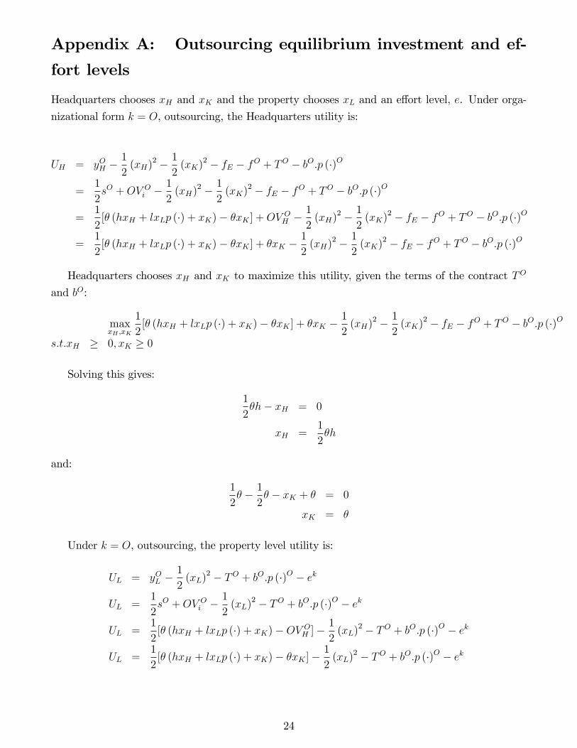
Headquarters chooses xH and xK and the property chooses xL and an e¤ort level, e. Under orga-

nizational form k = O, outsourcing, the Headquarters utility is:

UH = yOH �1

2(xH)

2 � 12(xK)

2 � fE � fO + TO � bO:p (�)O

=1

2sO +OV Oi �

1

2(xH)

2 � 12(xK)

2 � fE � fO + TO � bO:p (�)O

=1

2[� (hxH + lxLp (�) + xK)� �xK ] +OV OH �

1

2(xH)

2 � 12(xK)

2 � fE � fO + TO � bO:p (�)O

=1

2[� (hxH + lxLp (�) + xK)� �xK ] + �xK �

1

2(xH)

2 � 12(xK)

2 � fE � fO + TO � bO:p (�)O

Headquarters chooses xH and xK to maximize this utility, given the terms of the contract TO

and bO:

maxxH ;xK

1

2[� (hxH + lxLp (�) + xK)� �xK ] + �xK �

1

2(xH)

2 � 12(xK)

2 � fE � fO + TO � bO:p (�)O

s:t:xH � 0; xK � 0

Solving this gives:

1

2�h� xH = 0

xH =1

2�h

and:

1

2� � 1

2� � xK + � = 0

xK = �

Under k = O, outsourcing, the property level utility is:

UL = yOL �1

2(xL)

2 � TO + bO:p (�)O � ek

UL =1

2sO +OV Oi �

1

2(xL)

2 � TO + bO:p (�)O � ek

UL =1

2[� (hxH + lxLp (�) + xK)�OV OH ]�

1

2(xL)

2 � TO + bO:p (�)O � ek

UL =1

2[� (hxH + lxLp (�) + xK)� �xK ]�

1

2(xL)

2 � TO + bO:p (�)O � ek

24

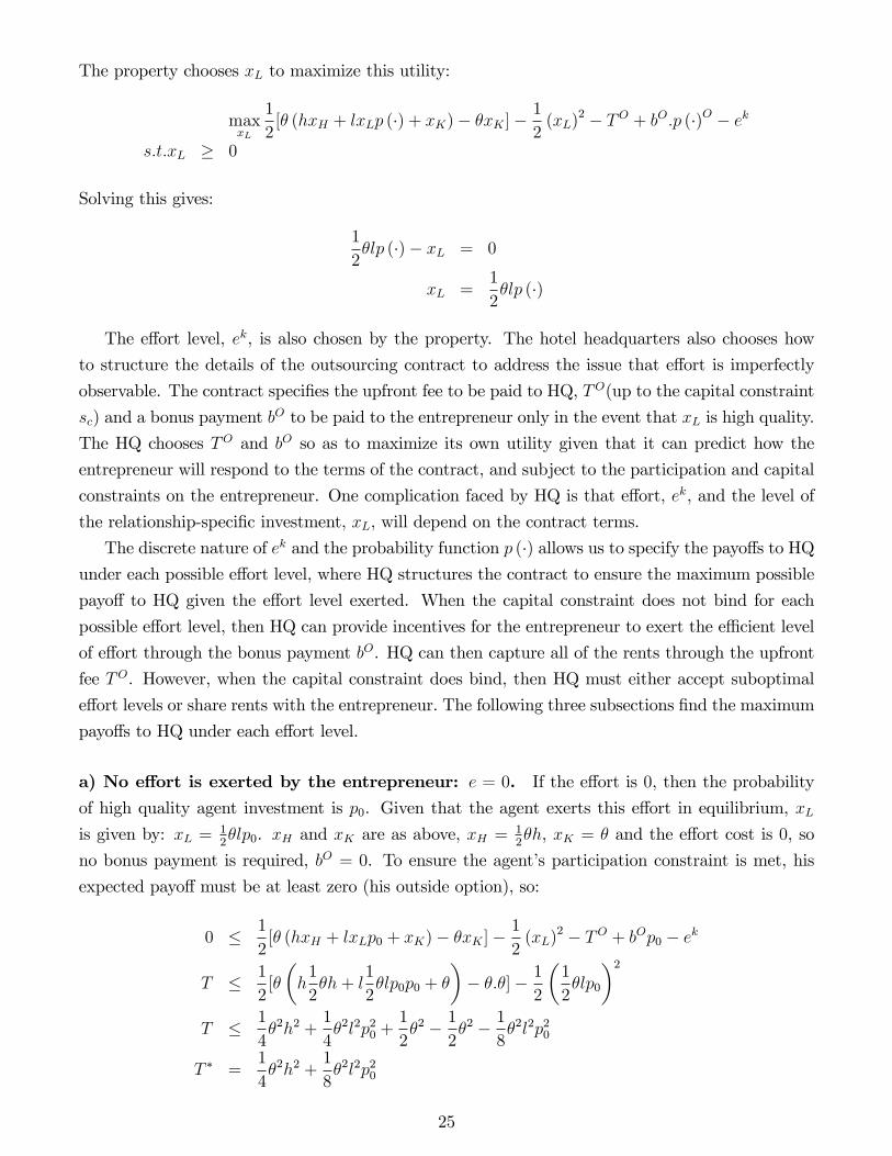
The property chooses xL to maximize this utility:

maxxL

1

2[� (hxH + lxLp (�) + xK)� �xK ]�

1

2(xL)

2 � TO + bO:p (�)O � ek

s:t:xL � 0

Solving this gives:

1

2�lp (�)� xL = 0

xL =1

2�lp (�)

The e¤ort level, ek, is also chosen by the property. The hotel headquarters also chooses how

to structure the details of the outsourcing contract to address the issue that e¤ort is imperfectly

observable. The contract speci�es the upfront fee to be paid to HQ, TO(up to the capital constraint

sc) and a bonus payment bO to be paid to the entrepreneur only in the event that xL is high quality.

The HQ chooses TO and bO so as to maximize its own utility given that it can predict how the

entrepreneur will respond to the terms of the contract, and subject to the participation and capital

constraints on the entrepreneur. One complication faced by HQ is that e¤ort, ek, and the level of

the relationship-speci�c investment, xL, will depend on the contract terms.

The discrete nature of ek and the probability function p (�) allows us to specify the payo¤s to HQunder each possible e¤ort level, where HQ structures the contract to ensure the maximum possible

payo¤ to HQ given the e¤ort level exerted. When the capital constraint does not bind for each

possible e¤ort level, then HQ can provide incentives for the entrepreneur to exert the e¢ cient level

of e¤ort through the bonus payment bO. HQ can then capture all of the rents through the upfront

fee TO. However, when the capital constraint does bind, then HQ must either accept suboptimal

e¤ort levels or share rents with the entrepreneur. The following three subsections �nd the maximum

payo¤s to HQ under each e¤ort level.

a) No e¤ort is exerted by the entrepreneur: e = 0. If the e¤ort is 0, then the probability

of high quality agent investment is p0. Given that the agent exerts this e¤ort in equilibrium, xLis given by: xL = 1

2�lp0. xH and xK are as above, xH = 1

2�h, xK = � and the e¤ort cost is 0, so

no bonus payment is required, bO = 0. To ensure the agent�s participation constraint is met, his

expected payo¤ must be at least zero (his outside option), so:

0 � 1

2[� (hxH + lxLp0 + xK)� �xK ]�

1

2(xL)

2 � TO + bOp0 � ek

T � 1

2[�

�h1

2�h+ l

1

2�lp0p0 + �

�� �:�]� 1

2

�1

2�lp0

�2T � 1

4�2h2 +

1

4�2l2p20 +

1

2�2 � 1

2�2 � 1

8�2l2p20

T � =1

4�2h2 +

1

8�2l2p20

25

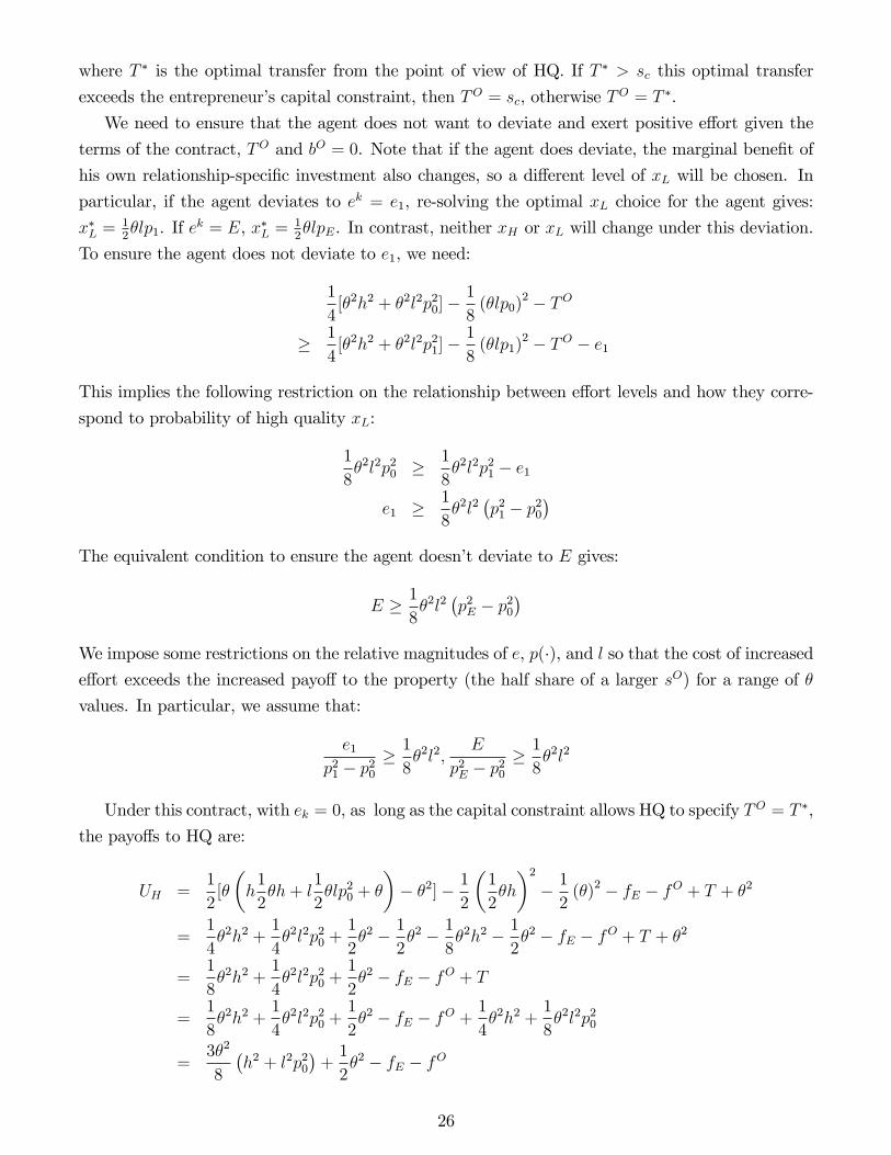
where T � is the optimal transfer from the point of view of HQ. If T � > sc this optimal transfer

exceeds the entrepreneur�s capital constraint, then TO = sc, otherwise TO = T �.

We need to ensure that the agent does not want to deviate and exert positive e¤ort given the

terms of the contract, TO and bO = 0. Note that if the agent does deviate, the marginal bene�t of

his own relationship-speci�c investment also changes, so a di¤erent level of xL will be chosen. In

particular, if the agent deviates to ek = e1, re-solving the optimal xL choice for the agent gives:

x�L =12�lp1. If ek = E, x�L =

12�lpE. In contrast, neither xH or xL will change under this deviation.

To ensure the agent does not deviate to e1, we need:

1

4[�2h2 + �2l2p20]�

1

8(�lp0)

2 � TO

� 1

4[�2h2 + �2l2p21]�

1

8(�lp1)

2 � TO � e1

This implies the following restriction on the relationship between e¤ort levels and how they corre-

spond to probability of high quality xL:

1

8�2l2p20 � 1

8�2l2p21 � e1

e1 � 1

8�2l2

�p21 � p20

�The equivalent condition to ensure the agent doesn�t deviate to E gives:

E � 1

8�2l2

�p2E � p20

�We impose some restrictions on the relative magnitudes of e, p(�), and l so that the cost of increasede¤ort exceeds the increased payo¤ to the property (the half share of a larger sO) for a range of �

values. In particular, we assume that:

e1p21 � p20

� 1

8�2l2;

E

p2E � p20� 1

8�2l2

Under this contract, with ek = 0, as long as the capital constraint allows HQ to specify TO = T �,

the payo¤s to HQ are:

UH =1

2[�

�h1

2�h+ l

1

2�lp20 + �

�� �2]� 1

2

�1

2�h

�2� 12(�)2 � fE � fO + T + �2

=1

4�2h2 +

1

4�2l2p20 +

1

2�2 � 1

2�2 � 1

8�2h2 � 1

2�2 � fE � fO + T + �2

=1

8�2h2 +

1

4�2l2p20 +

1

2�2 � fE � fO + T

=1

8�2h2 +

1

4�2l2p20 +

1

2�2 � fE � fO +

1

4�2h2 +

1

8�2l2p20

=3�2

8

�h2 + l2p20

�+1

2�2 � fE � fO

26

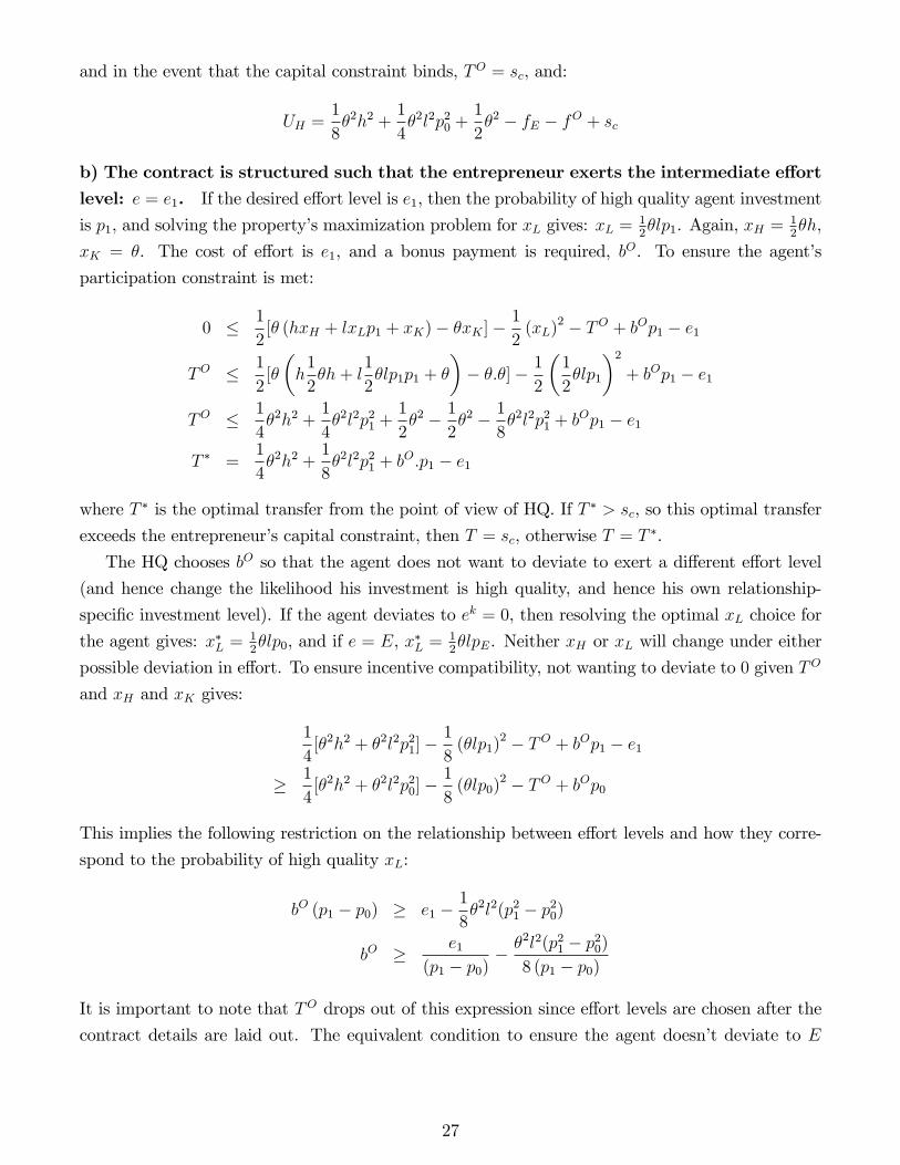
and in the event that the capital constraint binds, TO = sc, and:

UH =1

8�2h2 +

1

4�2l2p20 +

1

2�2 � fE � fO + sc

b) The contract is structured such that the entrepreneur exerts the intermediate e¤ortlevel: e = e1. If the desired e¤ort level is e1, then the probability of high quality agent investment

is p1, and solving the property�s maximization problem for xL gives: xL = 12�lp1. Again, xH = 1

2�h,

xK = �. The cost of e¤ort is e1, and a bonus payment is required, bO. To ensure the agent�s

participation constraint is met:

0 � 1

2[� (hxH + lxLp1 + xK)� �xK ]�

1

2(xL)

2 � TO + bOp1 � e1

TO � 1

2[�

�h1

2�h+ l

1

2�lp1p1 + �

�� �:�]� 1

2

�1

2�lp1

�2+ bOp1 � e1

TO � 1

4�2h2 +

1

4�2l2p21 +

1

2�2 � 1

2�2 � 1

8�2l2p21 + b

Op1 � e1

T � =1

4�2h2 +

1

8�2l2p21 + b

O:p1 � e1

where T � is the optimal transfer from the point of view of HQ. If T � > sc, so this optimal transfer

exceeds the entrepreneur�s capital constraint, then T = sc, otherwise T = T �.

The HQ chooses bO so that the agent does not want to deviate to exert a di¤erent e¤ort level

(and hence change the likelihood his investment is high quality, and hence his own relationship-

speci�c investment level). If the agent deviates to ek = 0, then resolving the optimal xL choice for

the agent gives: x�L =12�lp0, and if e = E, x�L =

12�lpE. Neither xH or xL will change under either

possible deviation in e¤ort. To ensure incentive compatibility, not wanting to deviate to 0 given TO

and xH and xK gives:

1

4[�2h2 + �2l2p21]�

1

8(�lp1)

2 � TO + bOp1 � e1

� 1

4[�2h2 + �2l2p20]�

1

8(�lp0)

2 � TO + bOp0

This implies the following restriction on the relationship between e¤ort levels and how they corre-

spond to the probability of high quality xL:

bO (p1 � p0) � e1 �1

8�2l2(p21 � p20)

bO � e1(p1 � p0)

� �2l2(p21 � p20)8 (p1 � p0)

It is important to note that TO drops out of this expression since e¤ort levels are chosen after the

contract details are laid out. The equivalent condition to ensure the agent doesn�t deviate to E

27

gives:

1

4[�2h2 + �2l2p21]�

1

8(�lp1)

2 � T + bOp1 � e1

� 1

4[�2h2 + �2l2p2E]�

1

8(�lpE)

2 � T + bOpE � E

This implies the following restriction on the relationship between e¤ort levels and how they corre-

spond to the probability of high quality xL:

bO (pE � p1) � E � e1 +1

8�2l2(p2E � p21)

bO � E � e1(pE � p1)

+�2l2(p2E � p21)8 (pE � p1)

Under the imposed assumptions about the relative size of e¤ort cost and return at di¤erent levels

of �, bO lies between these bounds and HQ will set:

bO =e1

(p1 � p0)� �

2l2(p21 � p20)8 (p1 � p0)

The payo¤s to HQ under this contract and e¤ort are, if the capital constraint does not bind are:

UH =1

2[�

�h1

2�h+ l

1

2�lp21 + �

�� �2]� 1

2

�1

2�h

�2� 12(�)2 � bOp1 � fE � fO + T + �2

=1

4�2h2 +

1

4�2l2p21 +

1

2�2 � 1

2�2 � 1

8�2h2 � 1

2�2 � bOp1 � fE � fO + T + �2

=1

8�2h2 +

1

4�2l2p21 +

1

2�2 � bOp1 � fE � fO + T

=1

8�2h2 +

1

4�2l2p21 +

1

2�2 � bOp1 � fE � fO +

1

4�2h2 +

1

8�2l2p21 + b

Op1 � e1

=3�2

8

�h2 + l2p21

�+1

2�2 � fE � fO � e1

noting that the bonus bO drops out of the payo¤. In the event that the capital constraint binds:

UH =1

8�2h2 +

1

4�2l2p21 +

1

2�2 � p1

�e1

(p1 � p0)� �

2l2(p21 � p20)8 (p1 � p0)

�� fE � fO + sc

c) The contract is structured such that the entrepreneur exerts the maximum e¤ortlevel: e = E. If the e¤ort is E, then the probability of high quality agent investment is pE and

xL is given by xL = 12�lpE. As above, xH = 1

2�h, and xK = �. The cost of e¤ort is E, and a bonus

28

payment is required, bO . To ensure the agent�s participation constraint is met:

0 � 1

2[� (hxH + lxLpE + xK)� �xK ]�

1

2(xL)

2 � TO + bOpE � E

TO � 1

2[�

�h1

2�h+ l

1

2�lpEpE + �

�� �:�]� 1

2

�1

2�lpE

�2+ bOpE � E

TO � 1

4�2h2 +

1

4�2l2p2E +

1

2�2 � 1

2�2 � 1

8�2l2p2E + b

OpE � E

T � =1

4�2h2 +

1

8�2l2p2E + b

OpE � E

where T � is the optimal transfer from the point of view of HQ. If T � > sc, so this optimal transfer

exceeds the entrepreneur�s capital constraint, then TO = sc, otherwise TO = T �.

The HQ chooses bO so that the agent does not want to deviate to exert a di¤erent e¤ort level

(and hence change the likelihood his investment is high quality, and hence his own relationship-

speci�c investment level). If the agent deviates to e = 0, then resolving the optimal xL choice for

the agent gives: x�L =12�lp0, and if e = e1, x�L =

12�lp1. Neither xH or xL will change. To ensure

incentive compatibility, not wanting to deviate to ek = 0 given TO and xH and xK gives:

1

4[�2h2 + �2l2p2E]�

1

8(�lpE)

2 � TO + bOpE � E

� 1

4[�2h2 + �2l2p20]�

1

8(�lp0)

2 � TO + bOp0

This implies the following restriction on the relationship between e¤ort levels and how they corre-

spond to the probability of high quality xL:

bO (pE � p0) � E � 18�2l2(p2E � p20)

bO � E

(pE � p0)� �

2l2(p2E � p20)8 (pE � p0)

As above, TO drops out since e¤ort levels are chosen after the contract details are laid out. The

equivalent condition to ensure the agent doesn�t deviate to e1 gives:

bO � E � e1(pE � p1)

� �2l2(p2E � p21)8 (pE � p1)

Under the imposed assumptions, the second of these restrictions binds �rst, so HQ will set:

bO =E � e1(pE � p1)

� �2l2(p2E � p21)8 (pE � p1)

The payo¤s to HQ under this contract and e¤ort are, if the capital constraint does not bind

29

(note bonus drops out):

UH =1

2[�

�h1

2�h+ l

1

2�lp2E + �

�� �2]� 1

2

�1

2�h

�2� 12(�)2 � bOpE � fE � fO + TO + �2

=1

4�2h2 +

1

4�2l2p2E +

1

2�2 � 1

2�2 � 1

8�2h2 � 1

2�2 � bOpE � fE � fO + TO + �2

=1

8�2h2 +

1

4�2l2p2E +

1

2�2 � bOpE � fE � fO + TO

=1

8�2h2 +

1

4�2l2p2E +

1

2�2 � bOpE � fE � fO +

1

4�2h2 +

1

8�2l2p2E + b

Op1 � E

=3�2

8

�h2 + l2p2E

�+1

2�2 � fE � fO � E

and in the event that the capital constraint binds:

UH =1

8�2h2 +

1

4�2l2p2E +

1

2�2 � pE

�E � e1(pE � p1)

� �2l2(p2E � p21)8 (pE � p1)

�� fE � fO + sc

7 Appendix B: Vertical Integration equilibrium investment

and e¤ort levels

The utility functions for each party under vertical integration re�ect the fact that HQ can monitor

directly, and contract upon, the e¤ort level exerted by the property on a fraction � of the required

tasks. We denote pm as the contribution to the probability local level is high quality made by

the fraction � of monitorable tasks, em. pn denotes the the equivalent for the fraction (1 � �) ofnon-monitorable tasks, en. In addition, there is no upfront transfer T from the property to HQ,

to capture the intuition that HQ cannot specify a negative wage for the property manager. The

contract sets out the required e¤ort level, and a bonus payment, bI , to be paid if the property level

investment is high quality. As outlined above, the surplus generated, sI , di¤ers re�ecting the fact

that HQ�s outside value is non-zero under VI.

Under organizational form k = I, vertical integration, the Headquarters utility is:

UH = yIH �1

2(xH)

2 � 12(xK)

2 � fE � f I � bIp (�)

=1

2sI +OV Ii �

1

2(xH)

2 � 12(xK)

2 � fE � f I � bIp (�)

=1

2[� (hxH + l�xLpm + l (1� �)xLpn + xK)� �xK � �� (hxH + l�xLpm + l (1� �)xLpn)]

�12(xH)

2 � 12(xK)

2 � fE � f I � bIp (�) + �xK + �� (hxH + l�xLpm + l (1� �)xLpn)

Headquarters chooses xH and xK to maximize this utility, given the terms of the contract em, and

30

hence pm, and bI :

maxxH ;xK

1

2[� (hxH + l�xLpm + l (1� �)xLpn + xK)� �xK � �� (hxH + l�xLpm + l (1� �)xLpn)]

�12(xH)

2 � 12(xK)

2 � fE � f I + T � bIp (�) + �xK + �� (hxH + l�xLpm + l (1� �)xLpn)s:t:xH � 0; xK � 0

Solving this gives:

1

2�h� 1

2��h� xH + ��h = 0

xH =1

2(1 + �) �h

and:

1

2� � 1

2� � xK + � = 0

xK = �

Under organizational form k = I, vertical integration, the property�s utility is:

UL = yIL �1

2(xL)

2 + bIp (�)� eI

UL =1

2[� (hxH + l�xLpm + l (1� �)xLpn + xK)� �xK � �� (hxH + l�xLpm + l (1� �)xLpn)]

�12(xL)

2 + bIp (�)� eI

The property chooses xL to maximize this utility:

maxxL

1

2[� (hxH + l�xLpm + l (1� �)xLpn + xK)� �xK � �� (hxH + l�xLpm + l (1� �)xLpn)]

�12(xL)

2 � T + b:p (�)� eI

s:t:xL � 0

Solving this gives:

1

2�(l�pm + l (1� �) pn)�

1

2�� (l�pm + l (1� �) pn)� xL = 0

xL =1

2(1� �) � (l�pm + l (1� �) pn)

We now turn to discuss how this standard property rights model result interacts with the e¤ect

of the discrete probability distribution p (�), the e¤ort exerted by the property. Since there are threepossible e¤ort levels for each task, and the manager can choose to exert a di¤erent amount of e¤ort

on the groups of non-monitored tasks to that which he is contracted to exert on monitored tasks,

31

there are nine possible combinations of overall e¤ort level that can be exerted. In each case, the

bonus payment must ensure that the manager�s expected payo¤ satis�es his participation and the

equilibrium e¤ort levels satisfy his incentive compatibility constraints.

a) i) The contract is structured so that em = 0 and en = 0. No bonus payment is re-

quired since no e¤ort is exerted on non-monitorable tasks. We know that xH = 12(1 + �) �h and

xK = �. If the manager exerts the desired e¤ort, then xL = 12(1� �) � (l�p0 + l (1� �) p0) =

12(1� �) �l (�p0 + (1� �) p0). Setting p = (�p0 + (1� �) p0) for this scenario only, we can writexL =

12(1� �) �lp. The manager�s utility is:

UL = yIL �1

2(xL)

2

UL =1

2[� (hxH + l�xLpm + l (1� �)xLpn + xK)� �xK � �� (hxH + l�xLpm + l (1� �)xLpn)]�

1

2(xL)

2

UL =1

2[� (hxH + lxL(�pm + (1� �) pn) + xK)� �xK � �� (hxH + lxL(�pm + (1� �) pn))]�

1

2(xL)

2

UL =1

2[� (hxH + lxLp+ �)� �2 � �� (hxH + lxLp)]�

1

2(xL)

2

UL =1

2[� (hxH + lxLp)� �� (hxH + lxLp)]�

1

2(xL)

2

UL =1

2[� (1� �) (hxH + lxLp)]�

1

2(xL)

2

UL =1

2[� (1� �) (hxH + lxLp)]�

1

2(xL)

2

UL =1

4[� (1� �)

�(1 + �) �h2 + l2 (1� �) � (�p0 + (1� �) p0) p

�]� 1

8((1� �) �lp)2

UL =1

4[�2h2 (1� �) (1 + �) + �2l2 (1� �)2 p (�p0 + (1� �) p0)]�

1

8(1� �)2 �2l2 (�p0 + (1� �) p0) p

=1

4�2 (1� �)

�h2 (1 + �) +

l2

2(1� �) p2

�This expected payo¤ satis�es the participation constraint since pand � are [0; 1]. To ensure that

the manager does not want to deviate and exert non-negative e¤ort, we need to check the following

two incentive compatibility constraints. If en = e1, so that xL = 12(1� �) � (l�p0 + l (1� �) p1) =

12(1� �) �p1, where p1 = (�p0 + (1� �) p1), and xH and xK are unchanged, the manager�s payo¤is:

UL =1

4�2 (1� �)

�h2 (1 + �) +

l2

2(1� �) p21

�� (1� �) e1

To ensure he does not want to deviate, we need that:

1

4�2 (1� �)

�l2

2(1� �) p2

�� 1

4�2 (1� �)

�l2

2(1� �) p21

�� (1� �) e1

e1 � �2l2 (1� �)2

8 (1� �)�p21 � p2

�

32

We need a similar condition to ensure the manager does not want to deviate to en = E:

E � �2l2 (1� �)2

8 (1� �)�p2E � p2

�where pE = (�p0 + (1� �) pE).The payo¤ to HQ is:

UH = yIH �1

2(xH)

2 � 12(xK)

2 � fE � f I � bIp (�)

=1

2sI +OV Ii �

1

2(xH)

2 � 12(xK)

2 � fE � f I � bIp (�)

=1

2[� (hxH + l�xLpm + l (1� �)xLpn + xK)� �xK � �� (hxH + l�xLpm + l (1� �)xLpn)]

�12(xH)

2 � 12(xK)

2 � fE � f I + �xK + �� (hxH + l�xLpm + l (1� �)xLpn)

=1

2[� (1� �)hxH + � (1� �) lxLp]�

1

2(xH)

2

�12(xK)

2 � fE � f I + �xK + �� (hxH + l�xLpm + l (1� �)xLpn)

=�

2(1 + �) [hxH + lxLp]�

1

2(xH)

2 � 12(xK)

2 � fE � f I + �xK

=�

2(1 + �) [hxH + lxLp]�

1

2(xH)

2 +1

2�2 � fE � f I

=�

2(1 + �)

�h1

2(1 + �) �h+ l

1

2(1� �) �lpp

�� 12

�1

2(1 + �) �h

�2+1

2�2 � fE � f I

=�2

4(1 + �)2 h2 +

�2

4(1 + �) (1� �) l2p2 � 1

8(1 + �)2 �2h2 +

1

2�2 � fE � f I

=�2h2

8(1 + �)2 +

�2l2

4(1 + �) (1� �) p2 + 1

2�2 � fE � f I

a) ii) The contract is structured so that em = 0 and en = e1. In this case, pm = p0 and

pn = p1.Rede�ne p = (�p0 + (1� �) p1). xH = 12(1 + �) �h, xL = 1

2(1� �) �lp and xH = �.

The speci�ed bonus, bI , needs to ensure that the expected payo¤ to the manager is positive and

also that he doesn�t want to deviate to en = 0, or en = E. The payo¤ to the manager if he doesn�t

deviate is:

UL =1

4�2 (1� �)

�h2 (1 + �) +

l2

2(1� �) p2

�+ bIp� (1� �) e1

If the manager were to deviate to en = 0, let p0 = (�p0 + (1� �) p0):

UL =1

4�2 (1� �)

�h2 (1 + �) +

l2

2(1� �) p20

�+ bIp0

33

Hence we need:

1

4�2 (1� �)

�l2

2(1� �) p2

�+ bIp� (1� �) e1 � 1

4�2 (1� �)

�l2

2(1� �) p20

�+ bIp0

bI (p� p0) � (1� �) e1 �1

8�2l2 (1� �)2

�p2 � p20

�bI � (1� �) e1

(p� p0)� �

2l2 (1� �)2

8 (p� p0)�p2 � p20

�For the manager to not deviate upwards and exert en = E, to obtain, where pE = (�p0 + (1� �) pE):

UL =1

4�2 (1� �)

�h2 (1 + �) +

l2

2(1� �) p2E

�+ bIpE � (1� �)E

we require

1

4�2 (1� �)

�l2

2(1� �) p2

�+ bIp� (1� �) e1 � 1

4�2 (1� �)

�l2

2(1� �) p2E

�+ bIpE � (1� �)E

bI (pE � p) � (1� �) (E � e1)�1

8�2l2 (1� �)2

�p2E � p2

�bI � (1� �) (E � e1)

(pE � p)� �

2l2 (1� �)2

8 (pE � p)�p2E � p2

�Under our assumptions, these conditions put upper and lower bounds on the bonus required (also

need to ensure expected manager payo¤ is non-negative). HQ will hence set the bonus at:

bI =(1� �) e1(p� p0)

� �2l2 (1� �)2

8 (p� p0)�p2 � p20

�To ensure that this the expected payo¤ to the manager is positive, given this bonus payment, we

need:

UL =1

4�2 (1� �)

�h2 (1 + �) +

l2

2(1� �) p2

�+p

"(1� �) e1(p� p0)

� �2l2 (1� �)2

8 (p� p0)�p2 � p20

�#�(1� �) e1 > 0

Under our imposed assumptions, we can show that this holds.

Under these contractual terms, the payo¤ to HQ is:

UH =�

2(1 + �) [hxH + lxLp]�

1

2(xH)

2 +1

2�2 � fE � f I � bIp

=�

2(1 + �)

�h1

2(1 + �) �h+ l

1

2(1� �) �lpp

�� 12

�1

2(1 + �) �h

�2+1

2�2 � fE � f I � bIp

=�2h2

4(1 + �)2 +

�2l2

4(1 + �) (1� �) p2 � �

2h2

8(1 + �)2 +

1

2�2 � fE � f I � bIp

=�2h2

8(1 + �)2 +

�2l2

4(1 + �) (1� �) p2 + 1

2�2 � fE � f I � p

"(1� �) e1(p� p0)

� �2l2 (1� �)2

8 (p� p0)�p2 � p20

�#

34

recalling that p in this expression di¤ers from p in scenario a)i).

a) iii) The contract is structured so that em = 0 and en = E. In this case, pm = p0 and

pn = pE. Let p = (�p0 + (1� �) pE). xH = 12(1 + �) �h, xL = 1

2(1� �) �lp and xH = �.

The bonus payment must ensure that the expected payo¤ to the manager is positive and that

he doesn�t want to deviate to en = 0, or en = e1. The payo¤ to the manager if he doesn�t deviate

is:

UL =1

4�2 (1� �)

�h2 (1 + �) +

l2

2(1� �) p2

�+ bIp� (1� �)E

If the manager were to deviate to en = 0, let p0 = (�p0 + (1� �) p0):

UL =1

4�2 (1� �)

�h2 (1 + �) +

l2

2(1� �) p20

�+ bIp0

Hence we need:

1

4�2 (1� �)

�l2

2(1� �) p2

�+ bIp� (1� �)E � 1

4�2 (1� �)

�l2

2(1� �) p20

�+ bIp0

bI (p� p0) � (1� �)E � 18�2l2 (1� �)2

�p2 � p20

�bI � (1� �)E

(p� p0)� �

2l2 (1� �)2

8 (p� p0)�p2 � p20

�For the manager to not deviate to e1, we need an equivalent condition on the bonus, where p1 =

(�p0 + (1� �) p1):

bI � (1� �) (E � e1)(p� p1)

� �2l2 (1� �)2

8 (p� p1)�p2 � p21

�Under our assumptions, these conditions put lower bounds on the bonus required , which mean that

the deviation to e1 is �rst to bind, so HQ sets:

bI =(1� �) (E � e1)

(p� p1)� �

2l2 (1� �)2

8 (p� p1)�p2 � p21

�To ensure that this the expected payo¤ to the manager is positive, given this bonus payment, we

need:

UL =1

4�2 (1� �)

�h2 (1 + �) +

l2

2(1� �) p2

�+p

"(1� �) (E � e1)

(p� p1)� �

2l2 (1� �)2

8 (p� p1)�p2 � p21

�#�(1� �)E > 0

Under our imposed assumptions, we can show that this holds.

35

The payo¤ to HQ is:

UH =�

2(1 + �) [hxH + lxLp]�

1

2(xH)

2 +1

2�2 � fE � f I � bIp

=�

2(1 + �)

�h1

2(1 + �) �h+ l

1

2(1� �) �lpp

�� 12

�1

2(1 + �) �h

�2+1

2�2 � fE � f I � bIp

=�2h2

4(1 + �)2 +

�2l2

4(1 + �) (1� �) p2 � �

2h2

8(1 + �)2 +

1

2�2 � fE � f I � bIp

=�2h2

8(1 + �)2 +

�2l2

4(1 + �) (1� �) p2 + 1

2�2 � fE � f I � p

"(1� �) (E � e1)

(p� p1)� �

2l2 (1� �)2

8 (p� p1)�p2 � p21

�#

(note that all the values containing a p di¤er from the previous two scenarios).

b) i) The contract is structured so that em = e1 and en = 0. As in a)i), no bonus payment

is required, but we need to ensure that the manager�s participation and incentive compatibility

conditions are satis�ed. We know that xH = 12(1 + �) �h and xK = �. If the manager exerts

the desired e¤ort, then xL = 12(1� �) � (l�p1 + l (1� �) p0) = 1

2(1� �) �l (�p1 + (1� �) p0). Set

p = (�p1 + (1� �) p0) for this case only, so xL = 12(1� �) �lp. The manager�s utility is:

UL = yIL �1

2(xL)

2 � �e1

UL =1

2[� (hxH + l�xLpm + l (1� �)xLpn + xK)� �xK � �� (hxH + l�xLpm + l (1� �)xLpn)]�

1

2(xL)

2 � �e1

UL =1

2[� (hxH + lxL(�pm + (1� �) pn) + xK)� �xK � �� (hxH + lxL(�pm + (1� �) pn))]�

1

2(xL)

2 � �e1

UL =1

2[� (hxH + lxLp+ �)� �2 � �� (hxH + lxLp)]�

1

2(xL)

2 � �e1

UL =1

2[� (hxH + lxLp)� �� (hxH + lxLp)]�

1

2(xL)

2 � �e1

UL =1

2[� (1� �) (hxH + lxLp)]�

1

2(xL)

2 � �e1

UL =1

2[� (1� �) (hxH + lxLp)]�

1

2(xL)

2 � �e1

UL =1

4[� (1� �)

�(1 + �) �h2 + l2 (1� �) � (�p1 + (1� �) p0) p

�]� 1

8((1� �) �lp)2 � �e1

UL =1

4[�2h2 (1� �) (1 + �) + �2l2 (1� �)2 p (�p1 + (1� �) p0)]�

1

8(1� �)2 �2l2 (�p1 + (1� �) p0) p� �e1

=1

4�2 (1� �)

�h2 (1 + �) +

l2

2(1� �) p2

�� �e1

We assume the �rst term in this expression outweighs the second, so that the participation constraint

is satis�ed. If the manager were to deviate so that en = e1, denoting p1 = (�p1 + (1� �) p1) so that

36

xL =12(1� �) � (l�p1 + l (1� �) p1) = 1

2(1� �) �p1, his payo¤ would be:

UL =1

4�2 (1� �)

�h2 (1 + �) +

l2

2(1� �) p21

�� �e1 � (1� �) e1

To ensure he does not want to deviate, we need that:

1

4�2 (1� �)

�l2

2(1� �) p2

�� �e1 � 1

4�2 (1� �)

�l2

2(1� �) p21

�� �e1 � (1� �) e1

e1 � �2l2 (1� �)2

8 (1� �)�p21 � p2

�We need a similar condition to ensure the manager does not want to deviate to en = E:

E � �2l2 (1� �)2

8 (1� �)�p2E � p2

�where pE = (�p1 + (1� �) pE).The payo¤ to HQ is:

UH = yIH �1

2(xH)

2 � 12(xK)

2 � fE � f I

=1

2sI +OV Ii �

1

2(xH)

2 � 12(xK)

2 � fE � f I

=1

2[� (hxH + l�xLpm + l (1� �)xLpn + xK)� �xK � �� (hxH + l�xLpm + l (1� �)xLpn)]�

1

2(xH)

2 � 12(xK)

2 � fE � f I + �xK + �� (hxH + l�xLpm + l (1� �)xLpn)

=1

2[� (1� �)hxH + � (1� �) lxLp]�

1

2(xH)

2 � 12(xK)

2 � fE � f I + �xK + �� (hxH + l�xLpm + l (1� �)xLpn)

=�

2(1 + �) [hxH + lxLp]�

1

2(xH)

2 � 12(xK)

2 � fE � f I + �xK

=�

2(1 + �) [hxH + lxLp]�

1

2(xH)

2 +1

2�2 � fE � f I

=�

2(1 + �)

�h1

2(1 + �) �h+ l

1

2(1� �) �lpp

�� 12

�1

2(1 + �) �h

�2+1

2�2 � fE � f I

=�2

4(1 + �)2 h2 +

�2

4(1 + �) (1� �) l2p2 � 1

8(1 + �)2 �2h2 +

1

2�2 � fE � f I

=�2h2

8(1 + �)2 +

�2l2

4(1 + �) (1� �) p2 + 1

2�2 � fE � f I

b) ii) The contract is structured so that em = e1 and en = e1. In this case, pm = p1 and

pn = p1. Let p = (�p1 + (1� �) p1). xH = 12(1 + �) �h, xL = 1

2(1� �) �lp and xH = �.

The payo¤ to the manager if he doesn�t deviate is:

UL =1

4�2 (1� �)

�h2 (1 + �) +

l2

2(1� �) p2

�+ bIp� �e1 � (1� �) e1

37

If the manager were to deviate to en = 0, denoting p0 = (�p0 + (1� �) p0), his payo¤ would be:

UL =1

4�2 (1� �)

�h2 (1 + �) +

l2

2(1� �) p20

�+ bIp0 � �e1

Hence we need:

1

4�2 (1� �)

�l2

2(1� �) p2

�+ bIp� (1� �) e1 � 1

4�2 (1� �)

�l2

2(1� �) p20

�+ bIp0

bI (p� p0) � (1� �) e1 �1

8�2l2 (1� �)2

�p2 � p20

�bI � (1� �) e1

(p� p0)� �

2l2 (1� �)2

8 (p� p0)�p2 � p20

�For the manager to not deviate upwards and obtain, where pE = (�p1 + (1� �) pE):

UL =1

4�2 (1� �)

�h2 (1 + �) +

l2

2(1� �) p2E

�+ bIpE � �e1 � (1� �)E

we require

1

4�2 (1� �)

�l2

2(1� �) p2

�+ bIp� �e1 � (1� �) e1 � 1

4�2 (1� �)

�l2

2(1� �) p2E

�+ bIpE � �e1 � (1� �)E

bI (pE � p) � (1� �) (E � e1)�1

8�2l2 (1� �)2

�p2E � p2

�bI � (1� �) (E � e1)

(pE � p)� �

2l2 (1� �)2

8 (pE � p)�p2E � p2

�Under our assumptions, these conditions put upper and lower bounds on the bonus required. HQ

will hence set the bonus at:

bI =(1� �) e1(p� p0)

� �2l2 (1� �)2

8 (p� p0)�p2 � p20

�Hence the payo¤ to the manager is:

UL =1

4�2 (1� �)

�h2 (1 + �) +

l2

2(1� �) p2

�+p

"(1� �) e1(p� p0)

� �2l2 (1� �)2

8 (p� p0)�p2 � p20

�#��e1�(1� �) e1

which our restrictions ensure is positive.

38

The payo¤ to HQ is:

UH =�

2(1 + �) [hxH + lxLp]�

1

2(xH)

2 +1

2�2 � fE � f I � bIp

=�

2(1 + �)

�h1

2(1 + �) �h+ l

1

2(1� �) �lpp

�� 12

�1

2(1 + �) �h

�2+1

2�2 � fE � f I � bIp

=�2h2

4(1 + �)2 +

�2l2

4(1 + �) (1� �) p2 � �

2h2

8(1 + �)2 +

1

2�2 � fE � f I � bIp

=�2h2

8(1 + �)2 +

�2l2

4(1 + �) (1� �) p2 + 1

2�2 � fE � f I � p

"(1� �) e1(p� p0)

� �2l2 (1� �)2

8 (p� p0)�p2 � p20

�#

(note that p is once again di¤erent).

b) iii) The contract is structured so that em = e1 and en = E. In this case, pm = p1 and

pn = pE. Let p = (�p1 + (1� �) pE). xH = 12(1 + �) �h, xL = 1

2(1� �) �lp and xH = �.

The payo¤ to the manager if he doesn�t deviate and exert less e¤ort on en is:

UL =1

4�2 (1� �)

�h2 (1 + �) +

l2

2(1� �) p2

�+ bIp� �e1 � (1� �)E

If the manager were to deviate to en = 0, denoting p0 = (�p1 + (1� �) p0):

UL =1

4�2 (1� �)

�h2 (1 + �) +

l2

2(1� �) p20

�� �e1 + bIp0

Hence we need:

1

4�2 (1� �)

�l2

2(1� �) p2

�+ bp� �e1 � (1� �)E � 1

4�2 (1� �)

�l2

2(1� �) p20

�+ bp0 � �e1

bI (p� p0) � (1� �)E � 18�2l2 (1� �)2

�p2 � p20

�bI � (1� �)E

(p� p0)� �

2l2 (1� �)2

8 (p� p0)�p2 � p20

�For the manager to not deviate to e1, we need an equivalent condition on the bonus, where p1 =

(�p1 + (1� �) p1):

bI � (1� �) (E � e1)(p� p1)

� �2l2 (1� �)2

8 (p� p1)�p2 � p21

�Under our assumptions, these conditions put lower bounds on the bonus required, which means

that the deviation to e1 is �rst to bind, so HQ sets:

bI =(1� �) (E � e1)

(p� p1)� �

2l2 (1� �)2

8 (p� p1)�p2 � p21

�

39

Hence the manager�s payo¤ is

UL =1

4�2 (1� �)

�h2 (1 + �) +

l2

2(1� �) p2

�+p

"(1� �) (E � e1)

(p� p1)� �

2l2 (1� �)2

8 (p� p1)�p2 � p21

�#��e1�(1� �)E

which our restrictions ensure is positive.

The payo¤ to HQ is:

UH =�

2(1 + �) [hxH + lxLp]�

1

2(xH)

2 +1

2�2 � fE � f I � bp

=�

2(1 + �)

�h1

2(1 + �) �h+ l

1

2(1� �) �lpp

�� 12

�1

2(1 + �) �h

�2+1

2�2 � fE � f I � bp

=�2h2

4(1 + �)2 +

�2l2

4(1 + �) (1� �) p2 � �

2h2

8(1 + �)2 +

1

2�2 � fE � f I � bp

=�2h2

8(1 + �)2 +

�2l2

4(1 + �) (1� �) p2 + 1

2�2 � fE � f I � p

"(1� �) (E � e1)

(p� p1)� �

2l2 (1� �)2

8 (p� p1)�p2 � p21

�#

(again p is di¤erent here).

c) i) The contract is structured so that em = E and en = 0. No bonus payment is required.

We know that xH = 12(1 + �) �h and xK = �. If the manager exerts the desired e¤ort, then

xL =12(1� �) � (l�p1 + l (1� �) p0) = 1

2(1� �) �l (�p1 + (1� �) p0). Set p = (�pE + (1� �) p0) for

this case only, so xL = 12(1� �) �lp. The manager�s utility is:

UL = yIL �1

2(xL)

2 � �E

UL =1

2[� (hxH + l�xLpm + l (1� �)xLpn + xK)� �xK � �� (hxH + l�xLpm + l (1� �)xLpn)]�

1

2(xL)

2 � �E

UL =1

2[� (hxH + lxL(�pm + (1� �) pn) + xK)� �xK � �� (hxH + lxL(�pm + (1� �) pn))]�

1

2(xL)

2 � �E

UL =1

2[� (hxH + lxLp+ �)� �2 � �� (hxH + lxLp)]�

1

2(xL)

2 � �E

UL =1

2[� (hxH + lxLp)� �� (hxH + lxLp)]�

1

2(xL)

2 � �E

UL =1

2[� (1� �) (hxH + lxLp)]�

1

2(xL)

2 � �E

UL =1

2[� (1� �) (hxH + lxLp)]�

1

2(xL)

2 � �E

UL =1

4[� (1� �)

�(1 + �) �h2 + l2 (1� �) � (�p1 + (1� �) p0) p

�]� 1

8((1� �) �lp)2 � �E

UL =1

4[�2h2 (1� �) (1 + �) + �2l2 (1� �)2 p (�p1 + (1� �) p0)]�

1

8(1� �)2 �2l2 (�p1 + (1� �) p0) p� �E

=1

4�2 (1� �)

�h2 (1 + �) +

l2

2(1� �) p2

�� �E

40

Our restrictions ensure this expression is positive. To ensure that he does not want to deviate and

exert positive e¤ort on non-monitorable tasks, we need to check the following two conditions: If en =

e1, denoting p1 = (�pE + (1� �) p1) so that xL = 12(1� �) � (l�pE + l (1� �) p1) = 1

2(1� �) �p1.

xH and xK are unchanged. The payo¤ to the manager is:

UL =1

4�2 (1� �)

�h2 (1 + �) +

l2

2(1� �) p21

�� �E � (1� �) e1

To ensure he does not want to deviate, we need that:

1

4�2 (1� �)

�l2

2(1� �) p2

�� �E � 1

4�2 (1� �)

�l2

2(1� �) p21

�� �E � (1� �) e1

e1 � �2l2 (1� �)2

8 (1� �)�p21 � p2

�We need a similar condition to ensure the manager does not want to deviate to en = E:

E � �2l2 (1� �)2

8 (1� �)�p2E � p2

�where pE = (�pE + (1� �) pE).The payo¤ to HQ is:

UH = yIH �1

2(xH)

2 � 12(xK)

2 � fE � f I

=1

2sI +OV Ii �

1

2(xH)

2 � 12(xK)

2 � fE � f I

=1

2[� (hxH + l�xLpm + l (1� �)xLpn + xK)� �xK � �� (hxH + l�xLpm + l (1� �)xLpn)]

�12(xH)

2 � 12(xK)

2 � fE � f I + �xK + �� (hxH + l�xLpm + l (1� �)xLpn)

=1

2[� (1� �)hxH + � (1� �) lxLp]

�12(xH)

2 � 12(xK)

2 � fE � f I + �xK + �� (hxH + l�xLpm + l (1� �)xLpn)

=�

2(1 + �) [hxH + lxLp]�

1

2(xH)

2 � 12(xK)

2 � fE � f I + �xK

=�

2(1 + �) [hxH + lxLp]�

1

2(xH)

2 +1

2�2 � fE � f I

=�

2(1 + �)

�h1

2(1 + �) �h+ l

1

2(1� �) �lpp

�� 12

�1

2(1 + �) �h

�2+1

2�2 � fE � f I

=�2

4(1 + �)2 h2 +

�2

4(1 + �) (1� �) l2p2 � 1

8(1 + �)2 �2h2 +

1

2�2 � fE � f I

=�2h2

8(1 + �)2 +

�2l2

4(1 + �) (1� �) p2 + 1

2�2 � fE � f I

41

c) ii) The contract is structured so that em = E and en = e1. In this case, pm = pE and

pn = p1 and p = (�pE + (1� �) p1). xH = 12(1 + �) �h, xL = 1

2(1� �) �lp and xH = �. The payo¤

to the manager if he doesn�t deviate is:

UL =1

4�2 (1� �)

�h2 (1 + �) +

l2

2(1� �) p2

�+ bIp� �E � (1� �) e1

If the manager were to deviate to en = 0, denoting p0 = (�pE + (1� �) p0):

UL =1

4�2 (1� �)

�h2 (1 + �) +

l2

2(1� �) p20

�+ bIp0 � �E

Hence we need:

1

4�2 (1� �)

�l2

2(1� �) p2

�+ bIp� (1� �) e1 � 1

4�2 (1� �)

�l2

2(1� �) p20

�+ bIp0

bI (p� p0) � (1� �) e1 �1

8�2l2 (1� �)2

�p2 � p20

�bI � (1� �) e1

(p� p0)� �

2l2 (1� �)2

8 (p� p0)�p2 � p20

�For the manager to not deviate upwards and obtain, where pE = (�pE + (1� �) pE):

UL =1

4�2 (1� �)

�h2 (1 + �) +

l2

2(1� �) p2E

�+ bIpE � �E � (1� �)E

we require

1

4�2 (1� �)

�l2

2(1� �) p2

�+ bIp� �E � (1� �) e1 � 1

4�2 (1� �)

�l2

2(1� �) p2E

�+ bIpE � �E � (1� �)E

bI (pE � p) � (1� �) (E � e1)�1

8�2l2 (1� �)2

�p2E � p2

�bI � (1� �) (E � e1)

(pE � p)� �

2l2 (1� �)2

8 (pE � p)�p2E � p2

�Under our assumptions, these conditions put upper and lower bounds on the bonus required. HQ

will hence set the bonus at:

bI =(1� �) e1(p� p0)

� �2l2 (1� �)2

8 (p� p0)�p2 � p20

�Hence the payo¤ to the manager is

UL =1

4�2 (1� �)

�h2 (1 + �) +

l2

2(1� �) p2

�+p

"(1� �) e1(p� p0)

� �2l2 (1� �)2

8 (p� p0)�p2 � p20

�#��E�(1� �) e1

which our restrictions ensure is positive.

42

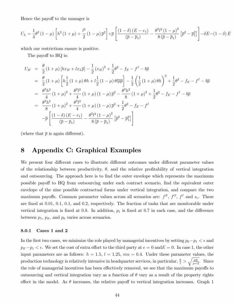
The payo¤ to HQ is:

UH =�

2(1 + �) [hxH + lxLp]�

1

2(xH)

2 +1

2�2 � fE � f I � bp

=�

2(1 + �)

�h1

2(1 + �) �h+ l

1

2(1� �) �lpp

�� 12

�1

2(1 + �) �h

�2+1

2�2 � fE � f I � bp

=�2h2

4(1 + �)2 +

�2l2

4(1 + �) (1� �) p2 � �

2h2

8(1 + �)2 +

1

2�2 � fE � f I � bp

=�2h2

8(1 + �)2 +

�2l2

4(1 + �) (1� �) p2 + 1

2�2 � fE � f I � p

"(1� �) e1(p� p0)

� �2l2 (1� �)2

8 (p� p0)�p2 � p20

�#

(note that p is again di¤erent).

c) iii) The contract is structured so that em = E and en = E. In this case, pm = pE and

pn = pE. Let p = (�pE + (1� �) pE). xH = 12(1 + �) �h, xL = 1

2(1� �) �lp and xH = �. The payo¤

to the manager if he doesn�t deviate is:

UL =1

4�2 (1� �)

�h2 (1 + �) +

l2

2(1� �) p2

�+ bp� �E � (1� �)E

If the manager were to deviate to en = 0, let p0 = (�p1 + (1� �) p0):

UL =1

4�2 (1� �)

�h2 (1 + �) +

l2

2(1� �) p20

�� �E + bp0

Hence we need:

1

4�2 (1� �)

�l2

2(1� �) p2

�+ bp� �E � (1� �)E � 1

4�2 (1� �)

�l2

2(1� �) p20

�+ bp0 � �E

b (p� p0) � (1� �)E � 18�2l2 (1� �)2

�p2 � p20

�b � (1� �)E

(p� p0)� �

2l2 (1� �)2

8 (p� p0)�p2 � p20

�For the manager to not deviate to e1, we need an equivalent condition on the bonus, where p1 =

(�pE + (1� �) p1):

b � (1� �) (E � e1)(p� p1)

� �2l2 (1� �)2

8 (p� p1)�p2 � p21

�Under our assumptions, these conditions put lower bounds on the bonus required (also need to

ensure expected manager payo¤ is non-negative), which mean that the deviation to e1 is �rst to

bind, so HQ sets:

b =(1� �) (E � e1)

(p� p1)� �

2l2 (1� �)2

8 (p� p1)�p2 � p21

�

43

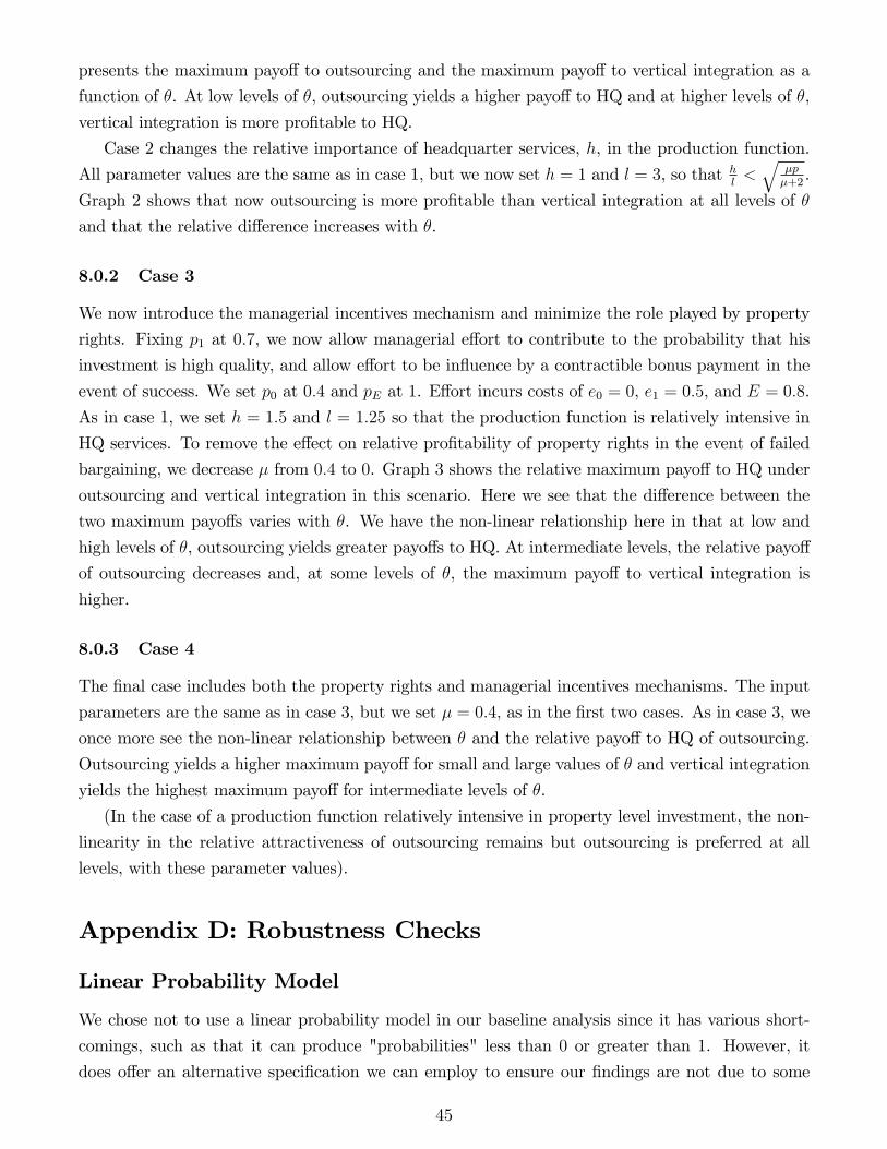
Hence the payo¤ to the manager is

UL =1

4�2 (1� �)

�h2 (1 + �) +

l2

2(1� �) p2

�+p

"(1� �) (E � e1)

(p� p1)� �

2l2 (1� �)2

8 (p� p1)�p2 � p21

�#��E�(1� �)E

which our restrictions ensure is positive.

The payo¤ to HQ is:

UH =�

2(1 + �) [hxH + lxLp]�

1

2(xH)

2 +1

2�2 � fE � f I � bp

=�

2(1 + �)

�h1

2(1 + �) �h+ l

1

2(1� �) �lpp

�� 12

�1

2(1 + �) �h

�2+1

2�2 � fE � f I � bp

=�2h2

4(1 + �)2 +

�2l2

4(1 + �) (1� �) p2 � �

2h2

8(1 + �)2 +

1

2�2 � fE � f I � bp

=�2h2

8(1 + �)2 +

�2l2

4(1 + �) (1� �) p2 + 1

2�2 � fE � f I

�p"(1� �) (E � e1)

(p� p1)� �

2l2 (1� �)2

8 (p� p1)�p2 � p21

�#

(where that p is again di¤erent).

8 Appendix C: Graphical Examples

We present four di¤erent cases to illustrate di¤erent outcomes under di¤erent parameter values

of the relationship between productivity, �, and the relative pro�tability of vertical integration

and outsourcing. The approach here is to �nd the outer envelope which represents the maximum

possible payo¤ to HQ from outsourcing under each contract scenario, �nd the equivalent outer

envelope of the nine possible contractual forms under vertical integration, and compare the two

maximum payo¤s. Common parameter values across all scenarios are: fE, fO, f I and sc. These

are �xed at 0:01, 0:1, 0:1, and 0:2, respectively. The fraction of tasks that are monitorable under

vertical integration is �xed at 0:8. In addition, p1 is �xed at 0:7 in each case, and the di¤erence

between p1, pE, and p0 varies across scenarios.

8.0.1 Cases 1 and 2

In the �rst two cases, we minimize the role played by managerial incentives by setting p0�p1 < � andpE�p1 < �. We set the cost of extra e¤ort to the third party at e = 0 andE = 0. In case 1, the otherinput parameters are as follows: h = 1:5, l = 1:25, mu = 0:4. Under these parameter values, the

production technology is relatively intensive in headquarter services, in particular, hl>q

�p�+2. Since

the role of managerial incentives has been e¤ectively removed, we see that the maximum payo¤s to

outsourcing and vertical integration vary as a function of � vary as a result of the property rights

e¤ect in the model. As � increases, the relative payo¤ to vertical integration increases. Graph 1

44

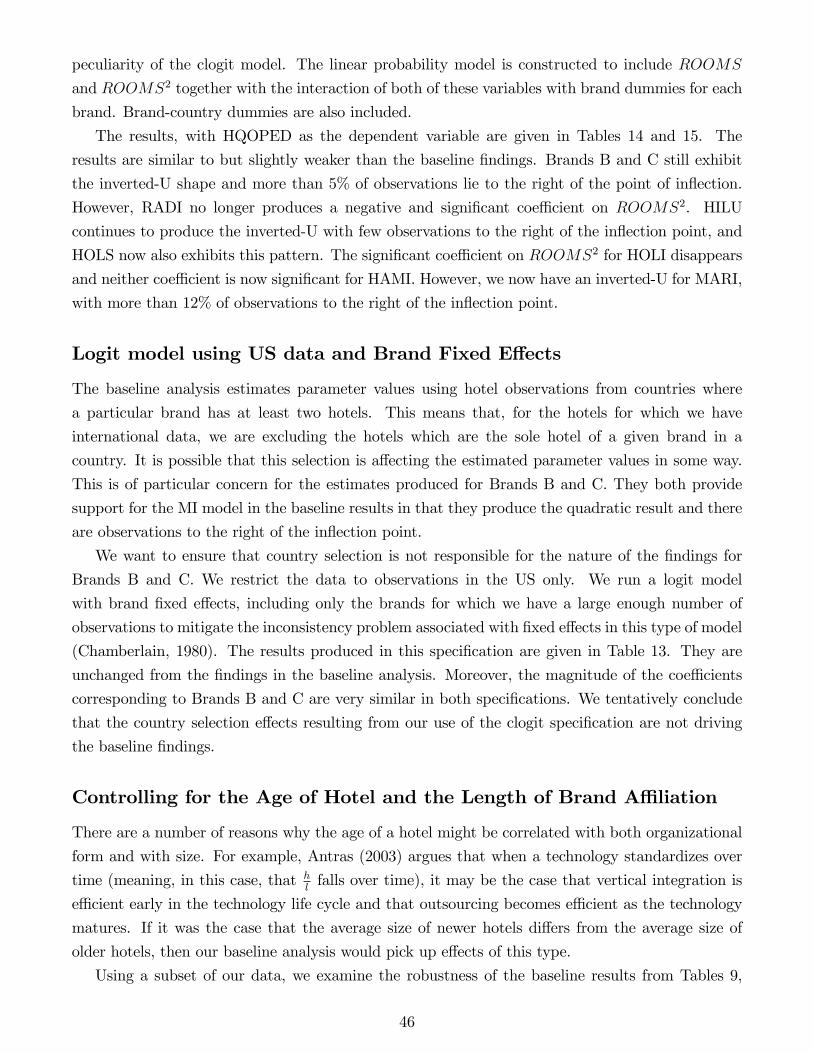
presents the maximum payo¤ to outsourcing and the maximum payo¤ to vertical integration as a

function of �. At low levels of �, outsourcing yields a higher payo¤ to HQ and at higher levels of �,

vertical integration is more pro�table to HQ.

Case 2 changes the relative importance of headquarter services, h, in the production function.

All parameter values are the same as in case 1, but we now set h = 1 and l = 3, so that hl<q

�p�+2.

Graph 2 shows that now outsourcing is more pro�table than vertical integration at all levels of �

and that the relative di¤erence increases with �.

8.0.2 Case 3

We now introduce the managerial incentives mechanism and minimize the role played by property

rights. Fixing p1 at 0:7, we now allow managerial e¤ort to contribute to the probability that his

investment is high quality, and allow e¤ort to be in�uence by a contractible bonus payment in the

event of success. We set p0 at 0:4 and pE at 1. E¤ort incurs costs of e0 = 0, e1 = 0:5, and E = 0:8.

As in case 1, we set h = 1:5 and l = 1:25 so that the production function is relatively intensive in

HQ services. To remove the e¤ect on relative pro�tability of property rights in the event of failed

bargaining, we decrease � from 0:4 to 0. Graph 3 shows the relative maximum payo¤ to HQ under

outsourcing and vertical integration in this scenario. Here we see that the di¤erence between the

two maximum payo¤s varies with �. We have the non-linear relationship here in that at low and

high levels of �, outsourcing yields greater payo¤s to HQ. At intermediate levels, the relative payo¤

of outsourcing decreases and, at some levels of �, the maximum payo¤ to vertical integration is

higher.

8.0.3 Case 4

The �nal case includes both the property rights and managerial incentives mechanisms. The input

parameters are the same as in case 3, but we set � = 0:4; as in the �rst two cases. As in case 3, we

once more see the non-linear relationship between � and the relative payo¤ to HQ of outsourcing.

Outsourcing yields a higher maximum payo¤ for small and large values of � and vertical integration

yields the highest maximum payo¤ for intermediate levels of �.

(In the case of a production function relatively intensive in property level investment, the non-

linearity in the relative attractiveness of outsourcing remains but outsourcing is preferred at all

levels, with these parameter values).

Appendix D: Robustness Checks

Linear Probability Model

We chose not to use a linear probability model in our baseline analysis since it has various short-

comings, such as that it can produce "probabilities" less than 0 or greater than 1. However, it

does o¤er an alternative speci�cation we can employ to ensure our �ndings are not due to some

45

peculiarity of the clogit model. The linear probability model is constructed to include ROOMS

and ROOMS2 together with the interaction of both of these variables with brand dummies for each

brand. Brand-country dummies are also included.

The results, with HQOPED as the dependent variable are given in Tables 14 and 15. The

results are similar to but slightly weaker than the baseline �ndings. Brands B and C still exhibit

the inverted-U shape and more than 5% of observations lie to the right of the point of in�ection.

However, RADI no longer produces a negative and signi�cant coe¢ cient on ROOMS2. HILU

continues to produce the inverted-U with few observations to the right of the in�ection point, and

HOLS now also exhibits this pattern. The signi�cant coe¢ cient on ROOMS2 for HOLI disappears

and neither coe¢ cient is now signi�cant for HAMI. However, we now have an inverted-U for MARI,

with more than 12% of observations to the right of the in�ection point.

Logit model using US data and Brand Fixed E¤ects

The baseline analysis estimates parameter values using hotel observations from countries where

a particular brand has at least two hotels. This means that, for the hotels for which we have

international data, we are excluding the hotels which are the sole hotel of a given brand in a

country. It is possible that this selection is a¤ecting the estimated parameter values in some way.

This is of particular concern for the estimates produced for Brands B and C. They both provide

support for the MI model in the baseline results in that they produce the quadratic result and there

are observations to the right of the in�ection point.

We want to ensure that country selection is not responsible for the nature of the �ndings for

Brands B and C. We restrict the data to observations in the US only. We run a logit model

with brand �xed e¤ects, including only the brands for which we have a large enough number of

observations to mitigate the inconsistency problem associated with �xed e¤ects in this type of model

(Chamberlain, 1980). The results produced in this speci�cation are given in Table 13. They are

unchanged from the �ndings in the baseline analysis. Moreover, the magnitude of the coe¢ cients

corresponding to Brands B and C are very similar in both speci�cations. We tentatively conclude

that the country selection e¤ects resulting from our use of the clogit speci�cation are not driving

the baseline �ndings.

Controlling for the Age of Hotel and the Length of Brand A¢ liation

There are a number of reasons why the age of a hotel might be correlated with both organizational

form and with size. For example, Antras (2003) argues that when a technology standardizes over

time (meaning, in this case, that hlfalls over time), it may be the case that vertical integration is

e¢ cient early in the technology life cycle and that outsourcing becomes e¢ cient as the technology

matures. If it was the case that the average size of newer hotels di¤ers from the average size of

older hotels, then our baseline analysis would pick up e¤ects of this type.

Using a subset of our data, we examine the robustness of the baseline results from Tables 9,

46

10, and 11 to the inclusion of controls for the age of each hotel. In particular, we make use of

the property-level age data in the secondary data. We estimate the following model of the latent

variable:

y0cbl = �cb + �11ROOMScbl +

BXz=2

[I(z = b)] �1zROOMScbl (10)

+�21 (ROOMScbl)2 +

BXz=2

[I(z = b)] �2z (ROOMScbl)2 (11)

+�3OPEN_MONTHScbl + �4AFFIL_MONTHScbl (12)

where �cb measures the e¤ect common to observations in the country c-brand b group, OPEN_MONTHScbl is

the number of months for which the l�th hotel property of the country c-brand b group has been

open, AFFIL_MONTHScbl is the equivalent number of months for which the hotel property has

been a¢ liated with the brand. All other variables and coe¢ cients are de�ned as before.

The results suggest that time since a¢ liation with current brand is strongly and positively cor-

related with the probability of HQ operational control. Column 2 of Table 14 shows estimates

of the full model (10). When OPEN_MONTHS and AFFIL_MONTHS are entered simul-

taneously, the coe¢ cient on OPEN_MONTHS is positive but insigni�cant, and the coe¢ cient

on AFFIL_MONTHS is positive and signi�cant at the 1 percent level.18 In general, the op-

eration of more recently a¢ liated properties are more likely to be outsourced. At the same time,

the estimates in Column 2 indicate that the key baseline results are robust to inclusion of con-

trols for hotel age. Table 15 shows the corresponding brand-speci�c coe¢ cients on ROOMS and

ROOMS2. The brand which produced the quadratic result with observations to the right of the

in�ection point in the baseline results - RADI - still does so once we include the controls for age

of hotel and length of brand a¢ liation. Of the three brands which produced the quadratic result

in the baseline analysis, but had very few observations to the right of the brand-speci�c in�ection

point, two continue to demonstrate these �ndings. These are HILU and HOLI. The linear result for

MARI in the baseline analysis remains unchanged. The baseline results change for only one brand,

HAMI. It exhibited the quadratic relationship in the baseline analysis but ceases to do so once the

age controls are included. The coe¢ cient on ROOMS2 is negative but not signi�cant. With these

estimates, the test for a within-sample inverted-U produces results similar to those in the baseline

analysis. Unfortunately, we are unable to test the robustness to age controls of the strongest results

�those for Brands B and C �because we do not at present have property-level age data for these

brand. However, as Table 16 indicates, for the 3 brands that exhibit a quadratic relationship, the

implied thresholds and distributions of observations around the thresholds change very little from

their baseline values.18We are unable at present to distinguish between age and time e¤ects, because we do not have observations for

the same hotels at di¤erent points in time. Older (as measured by a¢ liation dates) hotels may be more likely tobe operated by the HQ because technology de-standardizes as any given hotel ages. Alternatively, this correlationcould arise due to a secular shift towards outsourcing for newly built hotels.

47

Controlling for City Level Incidental Parameters

Our baseline speci�cation assumes that all error terms �cbl are independent and identically distrib-

uted. This will not be the case if there is a signi�cant city-level component in the parameters of

the underlying model. For example, if the headquarters�ability to monitor its managers varies from

city to city, even within brand-country groups, then the error terms for observations located in the

same city will have a common component. If this common component is correlated with hotel size,

we have a potential omitted variable bias. In order to mitigate the potential bias, we re-specify the

model and allow for city and brand e¤ects. In our �rst pass, we enter these group e¤ects separately

rather than interacting them; we group by city in a conditional logit framework and include brand

�xed e¤ects.

The results for HQOPED as the dependent variable are similar to the baseline estimates, with

one notable exception. Column 1 of Table 17 presents estimates of equation (8); it indicates

that the model predictions of a positive and signi�cant coe¢ cient on rooms and a negative and

signi�cant coe¢ cient on the square of the number of rooms do hold on average in the sample.

Column 2 presents estimates of equation (9), and Table 18 shows the corresponding brand-speci�c

coe¢ cients, standard errors, and p-values. Table 19 shows the proportion of observations included

in the analysis that fall to the left and to the right of the point of in�ection implied by the estimated

coe¢ cients on ROOMS and ROOMS2. Three important results obtain. First, of the 3 brands

that exhibited a signi�cant quadratic relationship in the baseline results and had more than 5% of

the observations included to the right of the in�ection point, 2 continue to do so once we control

for city e¤ects. These brands are Brand C and RADI. Brand B continues to exhibit the quadratic

relationship and has a large share of observations to the right of the calculated in�ection point,

but in this robustness check, the coe¢ cients on ROOMS and ROOMS2 interacted with the brand

dummy cease to be signi�cant. Data selection could be a contributing factor to the di¤erence in

the results for Brand B. Secondly, HAMI, HOLI and MARI continue to produce results consistent

with either theory in this robustness check. HAMI and HOLI continue to produce a quadratic

relationship with few observations to the right of the in�ection point. Third, HILU demonstrates

the quadratic relationship with both coe¢ cients signi�cant and around 4% of observations to the

right of the point of in�ection. MARI data yields a positive and signi�cant coe¢ cient on ROOMS

and an insigni�cant coe¢ cient on ROOMS2.

The broad similarity of these �ndings to our baseline results suggests that, while there are

city level factors in�uencing the estimated coe¢ cients, the qualitative baseline results are not a

spurious result of omitted variables that di¤er only across cities, nor are they driven by selection of

a particular subset of the sample. The results provide a small amount of evidence that is consistent

with the model only in the presence of managerial incentives, some evidence that is consistent with

either theory, and a small amount of evidence that is inconsistent with both theories.

Our next step is to carry out clogit estimation grouping the data by the interaction of brand

and city. This is the most conservative way of controlling for incidental parameters at the city level

since it allows the parameters to vary by brand. Unfortunately, this places severe restrictions on the

48

amount of data we can use. There are very few cities with more than one hotel of a given brand,

where organizational form varies for each hotel. This estimation is done using very few groups

and there tends to be few observations per group. Column 3 of Table 17 presents estimates of

equation (8). It shows that the model predictions of a positive and signi�cant coe¢ cient on rooms

and a negative and signi�cant coe¢ cient on the square of the number of rooms continue to hold in

the overall sample when controlling for brand-city group e¤ects. The estimation algorithm did not

converge when brand level interaction terms were included, most likely due to the lack of variation

in the data.

In the case that the error term component common to all observations in a given city is inde-

pendent of hotel size, we do not have a bias attributable to the city speci�c e¤ect. However, we

are required to cluster the data at the city level to allow for the non-independence of error terms.

The presence of city level factors, within country, would lead to the understatement of the standard

errors in our baseline clogit analysis and may cause us to falsely infer signi�cance. To ascertain

whether or not this is happening, we conduct an indicative test. Using only data from the US, we

compare the output of a pooled logit with that of a random e¤ects logit, where the data is grouped

at the city level. Very di¤erent results would suggest that city level factors are at work in the data.

The output of each estimation is given in Table 20. The random e¤ects logit output estimates

rho - the share of total variance explained by the city level component - to be around 10% in the

HQOPED case. Likelihood ratio tests suggested that this value of rho is signi�cantly di¤erent from

zero. Nonetheless, the overall results are unchanged in the random e¤ects speci�cation. Hypothesis

tests on the signi�cant of brand speci�c coe¢ cient estimates are given in Table 21. Table 22 presents

the share of observations lying to the right of the respective points of in�ection. The results are

very similar. We conclude that while there is a city level component to the error terms, it is not

large enough to lead us to draw false inference about the e¤ect of hotel size on organizational form

in our baseline analysis.

49

Table 21: Comparison of Pooled and RE Logit. US data only, brand fixed effects. Brand Specific Coefficients on Rooms and Rooms-Squared.

Coefficient Std Error p value Coefficient Std Error p valueBrand A Rooms 0.001420 0.002443 0.561000 0.002103 0.002624 0.423000

Rooms Squared 0.000001 0.000002 0.764000 0.000000 0.000002 0.885000

Brand B Rooms 0.073597 0.029199 0.012000 0.074135 0.031841 0.020000Rooms Squared -0.000144 0.000066 0.029000 -0.000147 0.000073 0.042000

HAMI Rooms 0.047074 0.014899 0.002000 0.060852 0.172918 0.000000Rooms Squared -0.000102 0.000052 0.048000 -0.000138 0.000058 0.017000

HAMS Rooms 0.289567 0.258307 0.262000 0.268649 0.254921 0.292000Rooms Squared -0.001267 0.001179 0.283000 -0.001184 0.001168 0.310000

HILU Rooms 0.014471 0.002616 0.000000 0.018631 0.003820 0.000000Rooms Squared -0.000004 0.000002 0.014000 -0.000007 0.000003 0.015000

HOLI Rooms 0.025184 0.005815 0.000000 0.024197 0.006327 0.000000Rooms Squared -0.000025 0.000008 0.004000 -0.000023 0.000009 0.013000

HOLS Rooms 0.334624 0.232125 0.149000 0.391204 0.257805 0.129000Rooms Squared -0.000604 0.000448 0.178000 -0.000703 0.000491 0.152000

HYAR Rooms 0.003212 0.008034 0.689000 0.003146 0.007027 0.654000Rooms Squared 0.000000 0.000006 0.948000 0.000000 0.000005 0.924000

HYAT Rooms 0.000374 0.011624 0.974000 -0.000187 0.011935 0.987000Rooms Squared 0.000003 0.000015 0.848000 0.000002 0.000012 0.888000

BRAND D Rooms -0.057168 0.084551 0.499000 0.000153 449.559700 1.000000Rooms Squared 0.000179 0.000257 0.486000 0.000000 0.616323 1.000000

MARI Rooms 0.006194 0.002124 0.004000 0.007802 0.002222 0.000000Rooms Squared -0.000002 0.000002 0.286000 -0.000003 0.000002 0.090000

RADI Rooms 0.031625 0.010959 0.004000 0.031373 0.012009 0.009000Rooms Squared -0.000031 0.000013 0.020000 -0.000030 0.000014 0.035000

BRAND C Rooms 0.025279 0.007295 0.001000 0.025611 0.007523 0.001000Rooms Squared -0.000017 0.000005 0.001000 -0.000017 0.000005 0.001000

Table 22: Comparison of Pooled and RE Logit. US data only, with brand fixed effects. Threshold Value of Rooms (Rooms*)

Panel A: Pooled Logit SpecificationDependent variable: HQOPED

Number of hotels with rooms: Share of observations with rooms:Brand Rooms* <Rooms* >=Rooms* Total <Rooms* >=Rooms*Brand B 256 134 17 151 88.7% 11.3%HAMI 230 1067 4 1071 99.6% 0.4%HAMS 114 96 61 157 61.1% 38.9%HILU 1936 213 2 215 99.1% 0.9%HOLI 511 819 9 828 98.9% 1.1%HOLS 277 54 4 58 93.1% 6.9%HYAR 4106 68 0 68 100.0% 0.0%MARI 1770 241 52 293 82.3% 17.7%RADI 509 222 11 233 95.3% 4.7%WEST 758 113 9 122 92.6% 7.4%

Panel B: Pooled Logit SpecificationDependent variable: HQOPED

Number of hotels with rooms: Share of observations with rooms:Brand Rooms* <Rooms* >=Rooms* Total <Rooms* >=Rooms*Brand B 252 133 18 151 88.1% 11.9%HAMI 221 1066 5 1071 99.5% 0.5%HAMS 113 96 61 157 61.1% 38.9%HILU 1378 207 8 215 96.3% 3.7%HOLI 527 820 8 828 99.0% 1.0%HOLS 278 54 4 58 93.1% 6.9%HYAR 3288 68 0 68 100.0% 0.0%MARI 1538 246 47 293 84.0% 16.0%RADI 522 223 10 233 95.7% 4.3%WEST 761 115 7 122 94.3% 5.7%

HQOPED - POOLED LOGIT HQOPED - RE Logit, grouping by city

Table 23: Analyis of HQOPED with "Gravity-Type" variables and brand fixed effectsPanel A: BRAND ANALYSIS: HQOPED, PRIMARY DATA

hqoped hqoped hqoped hqoped hqoped hqoped hqoped hqoped hqoped hqoped hqopeddistance_HQ 0.0003 0.0002 0.0002 0.0002 0.0002 0.0002 0.0003 0.0003 0.0002 0.0002

[0.0000393]*** [0.0000474]*** [0.0000469]*** [0.0000810]* [0.0000470]*** [0.0000654]*** [0.0000608]*** [0.0000600]*** [0.0001086]** [0.0000969]**1 is share legal family with HQ country -0.2021 -0.2497 -0.2349 -0.3153 -0.3103 -0.6183 -0.8668 -0.6832 -0.7677

[0.2514849] [0.2504382] [0.2498981] [0.2512152] [0.2512324] [0.3141185]** [0.2894805]*** [0.3201051]** [0.3387116]**density_group_city 0.1329 0.1043 0.1387

[0.0378762]*** [0.0487651]** [0.1392906]dist_group_density 0.0000 0.0000

[0.0000257] [0.0000399]density_brand_city 0.2211 0.1160 0.2274 0.2632

[0.0966731]** [0.1217297] [0.1543210] [0.2632519]dist_brand_density 0.0001 0.0000

[0.0000538] [0.0000744]Observations 990 990 990 990 990 990 653 653 654 653 653Standard errors in brackets* significant at 10%; ** significant at 5%; *** significant at 1%

Panel B:BRAND ANALYSIS: HQOPED, SECONDARY DATA

distance_HQ 0.0001 0.0002 0.0004 0.0002 0.0002 0.0003 0.0002[0.0001182] [0.0001190] [0.0002012]** [0.0001219]* [0.0001191] [0.0001756] [0.0001221]*

density_brand_city 0.2492 0.3545 0.2560[0.0439359]*** [0.0794576]*** [0.0453355]***

dist_brand_density -0.0001[0.0000951]

density_group_city 0.1216 0.1508 0.1263[0.0256824]*** [0.0481876]*** [0.0261598]***

dist_group_density 0.0000[0.0000645]

affil_months 0.0043 0.0043[0.0006295]*** [0.0006252]***

Observations 2478 2478 2478 2478 2478 2478 2478Standard errors in brackets* significant at 10%; ** significant at 5%; *** significant at 1%

US Hotels

Non-US HotelsAll Hotels

Table 24: Hotel Portfolio Characteristics, by Brand.

Panel A: Primary Data, Large Brands Only

BrandNumber of

Hotels Hotels in

USNon-US Hotels

Share HQOPED

overall

Share HQOPED

in US

Share HQOPED non-US

Number of Countries

Number of Countries with >1 Hotel

Average City Level Density

Average City

Density in US

Average City

Density Non US

Average City Level Density

Average City

Density in US

Average City

Density Non US

Average distance to HQ

%Common Legal Origin

%English speaking

Brand A 393 185 208 60% 42% 76% 68 30 1.58 1.66 1.51 2.41 2.84 1.99 3233 63% 58%Brand B 151 104 47 23% 20% 30% 18 8 1.17 1.17 1.14 2.31 2.25 2.46 1541 83% 83%Brand C 122 65 57 71% 80% 61% 25 11 1.37 1.50 1.20 3.46 4.34 2.33 2448 68% 70%Brand D 47 9 38 78% 78% 78% 21 6 1.29 1.00 1.35 2.32 2.43 2.29 4269 26% 26%Brand J 251 2 249 99% 100% 99% 43 20 2.63 1.00 2.65 2.84 4.00 2.83 2272 43% 42%Brand K 138 0 138 95% - 95% 9 7 3.59 - 3.59 3.92 - 3.92 818 0% 0%

Panel B: Secondary DataBrand Group

BrandNumber of

Hotels

Share HQOPED

overall

Average City Level Density

Average City Level Density

Average distance to HQ

Average Months Open

Average Affiliation

HAMI 1071 6% 1.76 2.29 626 111 102HAMS 157 3% 1.16 2.83 746 45 42HILU 215 31% 1.72 3.73 901 267 203HOLI 828 6% 1.68 1.75 741 336 267HOLS 58 7% 1.12 2.08 725 221 150HYAR 68 91% 1.17 1.49 886 250 234HYAT 47 89% 1.40 1.88 1050 271 168MARI 293 59% 1.99 1.99 990 214 163RADI 233 6% 1.56 1.56 957 289 104

Within Brand Within Group

Figure 1: Organizational form categories

Leased8 (primary)

Franchised300 (primary)2494 (secondary)

Owned179 (primary)

Managed/Rented552(primary)

HQOPED

HQOWND0 1

1

0

Chain Management

476 (secondary)

Figure 2: Pr(HQOWND) for US Hotels

0

0.2

0.4

0.6

0.8

1

1.2

0 to 50 51 to100

101 to150

151 to200

201 to250

251 to300

301 to350

351 to400

401 to450

451 to500

501 to550

551 to600

Morethan 600

Rooms Size Category

Brand ABrand BBrand C

Figure 3: Pr(HQOPED) for US Hotels

0

0.1

0.2

0.3

0.4

0.5

0.6

0.7

0.8

0.9

1

0 to 50 51 to100

101 to150

151 to200

201 to250

251 to300

301 to350

351 to400

401 to450

451 to500

501 to550

551 to600

Morethan 600

Rooms Size Category

HILURADIBrand BHOLIHOLS

Figure 4: Maximum Payoffs to VI and Outsourcing under Case 1

-1

0

1

2

3

4

5

6

7

8

9

1 11 21 31 41 51 61 71 81 91 101 111 121 131 141 151 161 171 181 191 201 211 221 231 241 251

Max payoff from VIMax payoff from Outsourcing

Figure 5: Maximum Payoffs to VI and Outsourcing under Case 2

-5

0

5

10

15

20

1 11 21 31 41 51 61 71 81 91 101 111 121 131 141 151 161 171 181 191 201 211 221 231 241 251

Max payoff from VIMax payoff from Outsourcing

Figure 6: Maximum Payoffs to VI and Outsourcing under Case 3

-1

0

1

2

3

4

5

6

7

8

9

10

1 11 21 31 41 51 61 71 81 91 101 111 121 131 141 151 161 171 181 191 201 211 221 231 241 251

Max payoff from VIMax payoff from Outsourcing

Figure 7: Maximum Payoffs to VI and Outsourcing under Case 4

-1

0

1

2

3

4

5

6

7

8

9

10

1 11 21 31 41 51 61 71 81 91 101 111 121 131 141 151 161 171 181 191 201 211 221 231 241 251

Max payoff from VIMax payoff from Outsourcing