Embed Size (px)
Citation preview
When are scale-free graphs ultra-small?
Julia Komjathy
joint with Remco van der HofstadEindhoven University of Technology
Probability Seminar in Bristol,Nov 4, 2016
Julia Komjathy 1 / 34
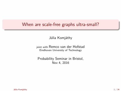
Complex networks 1.
IP level internet network, 2003from the OPTE project, opte.org
Julia Komjathy 2 / 34
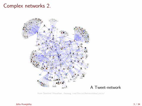
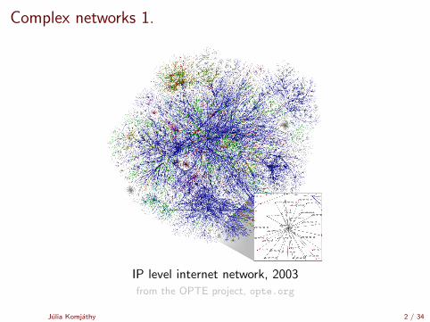
Complex networks 2.
A Tweet-networkfrom Sentinel Visualiser, fmsasg.com/SocialNetworkAnalysis/
Julia Komjathy 3 / 34

Degree plots
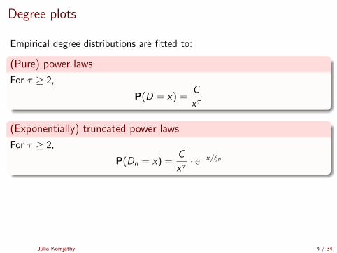
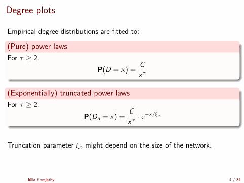
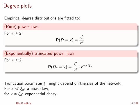
Empirical degree distributions are fitted to:
(Pure) power laws
For τ ≥ 2,
P(D = x) =C
xτ
(Exponentially) truncated power laws
For τ ≥ 2,
P(Dn = x) =C
xτ· e−x/ξn
Truncation parameter ξn might depend on the size of the network.For x � ξn: a power law,for x ≈ ξn: exponential decay.
Julia Komjathy 4 / 34

Degree plots
Empirical degree distributions are fitted to:
(Pure) power laws
For τ ≥ 2,
P(D = x) =C
xτ
(Exponentially) truncated power laws
For τ ≥ 2,
P(Dn = x) =C
xτ· e−x/ξn
Truncation parameter ξn might depend on the size of the network.For x � ξn: a power law,for x ≈ ξn: exponential decay.
Julia Komjathy 4 / 34
Degree plots
Empirical degree distributions are fitted to:
(Pure) power laws
For τ ≥ 2,
P(D = x) =C
xτ
(Exponentially) truncated power laws
For τ ≥ 2,
P(Dn = x) =C
xτ· e−x/ξn
Truncation parameter ξn might depend on the size of the network.
For x � ξn: a power law,for x ≈ ξn: exponential decay.
Julia Komjathy 4 / 34
Degree plots
Empirical degree distributions are fitted to:
(Pure) power laws
For τ ≥ 2,
P(D = x) =C
xτ
(Exponentially) truncated power laws
For τ ≥ 2,
P(Dn = x) =C
xτ· e−x/ξn
Truncation parameter ξn might depend on the size of the network.For x � ξn: a power law,for x ≈ ξn: exponential decay.
Julia Komjathy 4 / 34
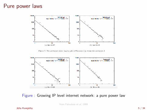
Pure power laws
Figure : Growing IP level internet network: a pure power law
from Faloutsos et al, 1999
Julia Komjathy 5 / 34
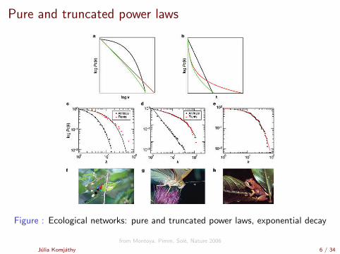
Pure and truncated power laws
Figure : Ecological networks: pure and truncated power laws, exponential decay
from Montoya, Pimm, Sole, Nature 2006
Julia Komjathy 6 / 34

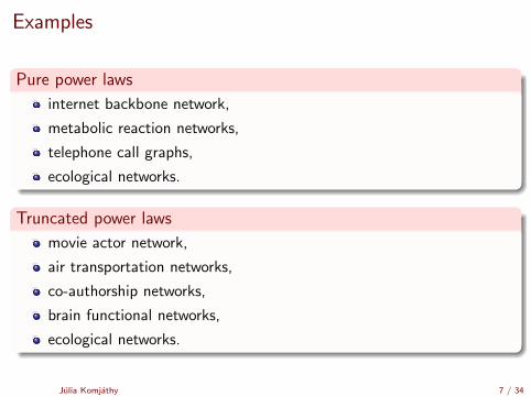
Examples
Pure power laws
internet backbone network,
metabolic reaction networks,
telephone call graphs,
ecological networks.
Truncated power laws
movie actor network,
air transportation networks,
co-authorship networks,
brain functional networks,
ecological networks.
Julia Komjathy 7 / 34

Examples
Pure power laws
internet backbone network,
metabolic reaction networks,
telephone call graphs,
ecological networks.
Truncated power laws
movie actor network,
air transportation networks,
co-authorship networks,
brain functional networks,
ecological networks.
Julia Komjathy 7 / 34
Examples
Pure power laws
internet backbone network,
metabolic reaction networks,
telephone call graphs,
ecological networks.
Truncated power laws
movie actor network,
air transportation networks,
co-authorship networks,
brain functional networks,
ecological networks.
Julia Komjathy 7 / 34
Scale free vs ultra small
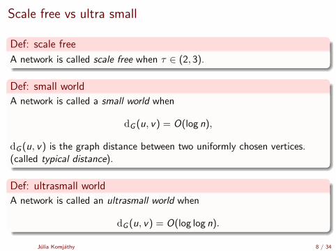
Def: scale free
A network is called scale free when τ ∈ (2, 3).
Def: small world
A network is called a small world when
dG (u, v) = O(log n),
dG (u, v) is the graph distance between two uniformly chosen vertices.(called typical distance).
Def: ultrasmall world
A network is called an ultrasmall world when
dG (u, v) = O(log log n).
Julia Komjathy 8 / 34
Scale free vs ultra small
Def: scale free
A network is called scale free when τ ∈ (2, 3).
Def: small world
A network is called a small world when
dG (u, v) = O(log n),
dG (u, v) is the graph distance between two uniformly chosen vertices.(called typical distance).
Def: ultrasmall world
A network is called an ultrasmall world when
dG (u, v) = O(log log n).
Julia Komjathy 8 / 34

Scale free?= ultra small
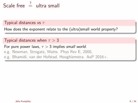
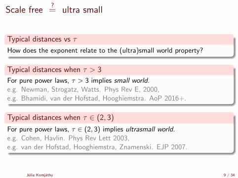
Typical distances vs τ
How does the exponent relate to the (ultra)small world property?
Typical distances when τ > 3
For pure power laws, τ > 3 implies small world.e.g. Newman, Strogatz, Watts. Phys Rev E, 2000,e.g. Bhamidi, van der Hofstad, Hooghiemstra. AoP 2016+.
Typical distances when τ ∈ (2, 3)
For pure power laws, τ ∈ (2, 3) implies ultrasmall world.e.g. Cohen, Havlin. Phys Rev Lett 2003,e.g. van der Hofstad, Hooghiemstra, Znamenski. EJP 2007.
Julia Komjathy 9 / 34
Scale free?= ultra small
Typical distances vs τ
How does the exponent relate to the (ultra)small world property?
Typical distances when τ > 3
For pure power laws, τ > 3 implies small world.e.g. Newman, Strogatz, Watts. Phys Rev E, 2000,e.g. Bhamidi, van der Hofstad, Hooghiemstra. AoP 2016+.
Typical distances when τ ∈ (2, 3)
For pure power laws, τ ∈ (2, 3) implies ultrasmall world.e.g. Cohen, Havlin. Phys Rev Lett 2003,e.g. van der Hofstad, Hooghiemstra, Znamenski. EJP 2007.
Julia Komjathy 9 / 34

Truncated scale free?= ultrasmall world
Goal of this talk
How does the truncation point ξn affect the ultrasmall world property?
Julia Komjathy 10 / 34

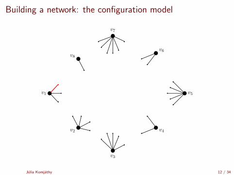
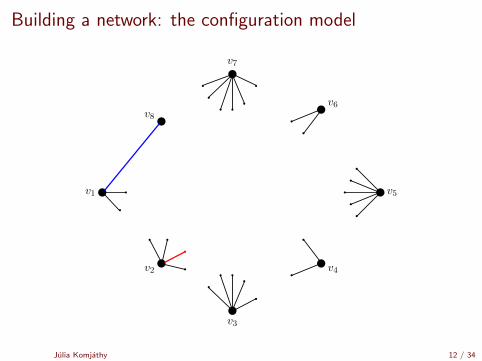
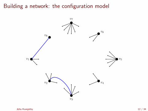
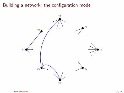
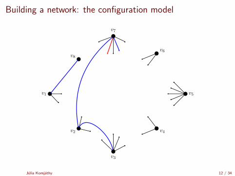
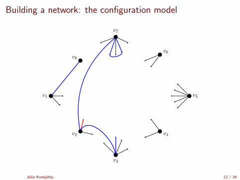
Building a network: the configuration model
[Uniform matching simulator by Robert Fitzner][Configuration model simulator by Robert Fitzner]
Julia Komjathy 11 / 34

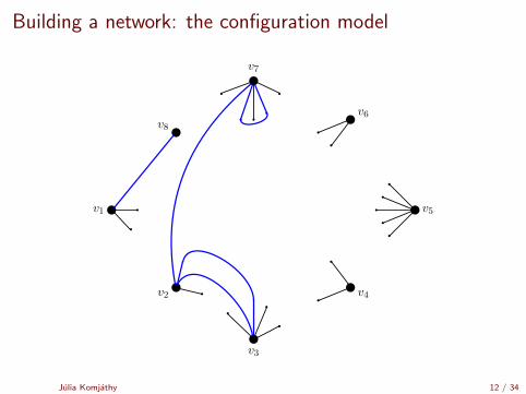
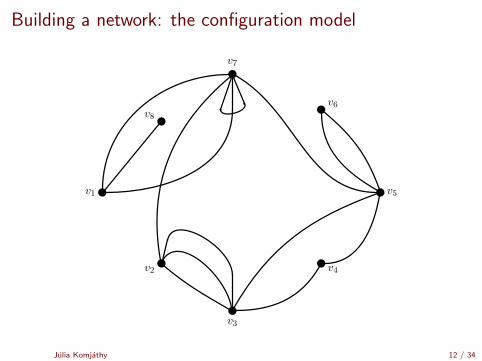
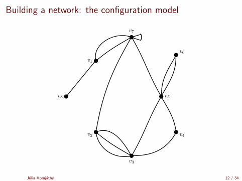
Building a network: the configuration model
v1
v2
v3
v4
v5
v8
v7
v6
Julia Komjathy 12 / 34
Building a network: the configuration model
v1
v2
v3
v4
v5
v8
v7
v6
Julia Komjathy 12 / 34

Building a network: the configuration model
v1
v2
v3
v4
v5
v8
v7
v6
Julia Komjathy 12 / 34

Building a network: the configuration model
v1
v2
v3
v4
v5
v8
v7
v6
Julia Komjathy 12 / 34
Building a network: the configuration model
v1
v2
v3
v4
v5
v8
v7
v6
Julia Komjathy 12 / 34

Building a network: the configuration model
v1
v2
v3
v4
v5
v8
v7
v6
Julia Komjathy 12 / 34
Building a network: the configuration model
v1
v2
v3
v4
v5
v8
v7
v6
Julia Komjathy 12 / 34

Building a network: the configuration model
v1
v2
v3
v4
v5
v8
v7
v6
Julia Komjathy 12 / 34

Building a network: the configuration model
v1
v2
v3
v4
v5
v8
v7
v6
Julia Komjathy 12 / 34
Building a network: the configuration model
v1
v2
v3
v4
v5
v8
v7
v6
Julia Komjathy 12 / 34

Building a network: the configuration model
v1
v2
v3
v4
v5
v8
v7
v6
Julia Komjathy 12 / 34
Building a network: the configuration model
v1
v2
v3
v4
v5
v8
v7
v6
Julia Komjathy 12 / 34

Building a network: the configuration model
v1
v2
v3
v4
v5
v8
v7
v6
Julia Komjathy 12 / 34

Building a network: the configuration model
v1
v2
v3
v4
v5
v8
v7
v6
Julia Komjathy 12 / 34
Building a network: the configuration model
v1
v2
v3
v4
v5
v8
v7
v6
Julia Komjathy 12 / 34
Building a network: the configuration model
v1
v2
v3
v4
v5
v8
v7
v6
Julia Komjathy 12 / 34
Building a network: the configuration model
v1
v2
v3
v4
v5
v8
v7
v6
Julia Komjathy 12 / 34
Building a network: the configuration model
v1
v2
v3
v4
v5v8
v7
v6
Julia Komjathy 12 / 34
Degree assumptions
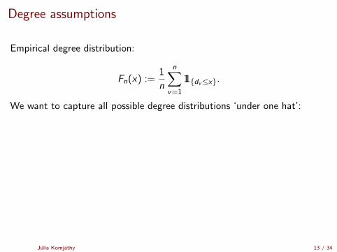
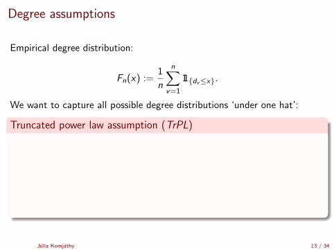
Empirical degree distribution:
Fn(x) :=1
n
n∑v=1
11{dv≤x}.
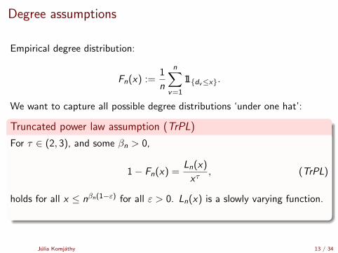
We want to capture all possible degree distributions ‘under one hat’:
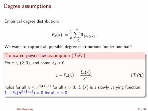
Truncated power law assumption (TrPL)
For τ ∈ (2, 3), and some βn > 0,
1− Fn(x) =Ln(x)
xτ, (TrPL)
holds for all x ≤ nβn(1−ε) for all ε > 0. Ln(x) is a slowly varying function.1− Fn(nβn(1+ε)) = 0 for all ε > 0.
Julia Komjathy 13 / 34
Degree assumptions
Empirical degree distribution:
Fn(x) :=1
n
n∑v=1
11{dv≤x}.
We want to capture all possible degree distributions ‘under one hat’:
Truncated power law assumption (TrPL)
For τ ∈ (2, 3), and some βn > 0,
1− Fn(x) =Ln(x)
xτ, (TrPL)
holds for all x ≤ nβn(1−ε) for all ε > 0. Ln(x) is a slowly varying function.
1− Fn(nβn(1+ε)) = 0 for all ε > 0.
Julia Komjathy 13 / 34
Degree assumptions
Empirical degree distribution:
Fn(x) :=1
n
n∑v=1
11{dv≤x}.
We want to capture all possible degree distributions ‘under one hat’:
Truncated power law assumption (TrPL)
For τ ∈ (2, 3), and some βn > 0,
1− Fn(x) =Ln(x)
xτ, (TrPL)
holds for all x ≤ nβn(1−ε) for all ε > 0. Ln(x) is a slowly varying function.1− Fn(nβn(1+ε)) = 0 for all ε > 0.
Julia Komjathy 13 / 34

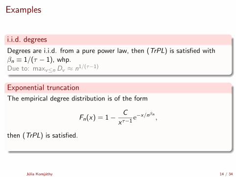
Examples
i.i.d. degrees
Degrees are i.i.d. from a pure power law, then (TrPL) is satisfied withβn ≡ 1/(τ − 1), whp.
Due to: maxv≤n Dv ≈ n1/(τ−1)
Exponential truncation
The empirical degree distribution is of the form
Fn(x) = 1− C
xτ−1e−x/n
βn,
then (TrPL) is satisfied.
Ex: dv := min{Dv ,Gv}, Dv ∼ D i.i.d. power law, Gv ∼ Geo(e−nβ
) i.i.d.
Julia Komjathy 14 / 34

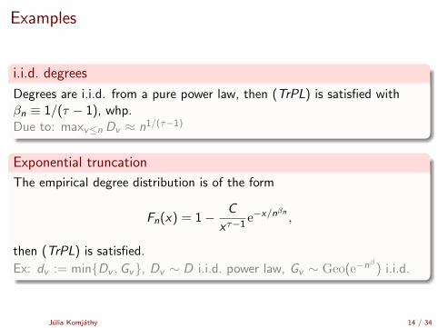
Examples
i.i.d. degrees
Degrees are i.i.d. from a pure power law, then (TrPL) is satisfied withβn ≡ 1/(τ − 1), whp.Due to: maxv≤n Dv ≈ n1/(τ−1)
Exponential truncation
The empirical degree distribution is of the form
Fn(x) = 1− C
xτ−1e−x/n
βn,
then (TrPL) is satisfied.
Ex: dv := min{Dv ,Gv}, Dv ∼ D i.i.d. power law, Gv ∼ Geo(e−nβ
) i.i.d.
Julia Komjathy 14 / 34

Examples 2.
Hard truncation
The empirical degree distribution is of the form
Fn(x) = 1− C
xτ−111x≤nβn ,
then (TrPL) is satisfied.
Ex: dv := min{Dv , nβn}, Dv ∼ D i.i.d. power law
Julia Komjathy 15 / 34

Examples 2.
Hard truncation
The empirical degree distribution is of the form
Fn(x) = 1− C
xτ−111x≤nβn ,
then (TrPL) is satisfied.Ex: dv := min{Dv , n
βn}, Dv ∼ D i.i.d. power law
Julia Komjathy 15 / 34
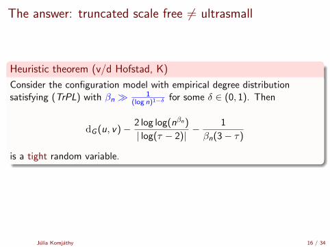
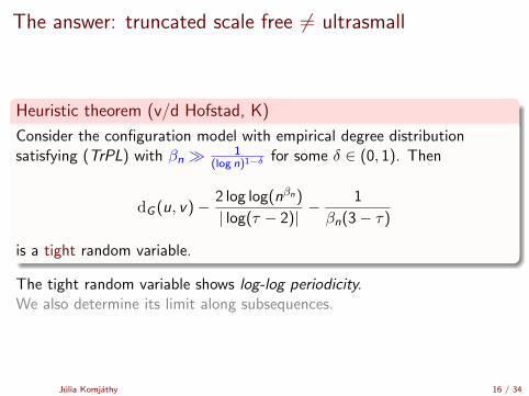
The answer: truncated scale free 6= ultrasmall
Heuristic theorem (v/d Hofstad, K)
Consider the configuration model with empirical degree distributionsatisfying (TrPL) with βn � 1
(log n)1−δ for some δ ∈ (0, 1). Then
dG (u, v)− 2 log log(nβn)
| log(τ − 2)|− 1
βn(3− τ)
is a tight random variable.
The tight random variable shows log-log periodicity.We also determine its limit along subsequences.
Julia Komjathy 16 / 34
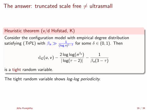
The answer: truncated scale free 6= ultrasmall
Heuristic theorem (v/d Hofstad, K)
Consider the configuration model with empirical degree distributionsatisfying (TrPL) with βn � 1
(log n)1−δ for some δ ∈ (0, 1). Then
dG (u, v)− 2 log log(nβn)
| log(τ − 2)|− 1
βn(3− τ)
is a tight random variable.
The tight random variable shows log-log periodicity.
We also determine its limit along subsequences.
Julia Komjathy 16 / 34
The answer: truncated scale free 6= ultrasmall
Heuristic theorem (v/d Hofstad, K)
Consider the configuration model with empirical degree distributionsatisfying (TrPL) with βn � 1
(log n)1−δ for some δ ∈ (0, 1). Then
dG (u, v)− 2 log log(nβn)
| log(τ − 2)|− 1
βn(3− τ)
is a tight random variable.
The tight random variable shows log-log periodicity.We also determine its limit along subsequences.
Julia Komjathy 16 / 34
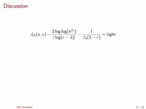
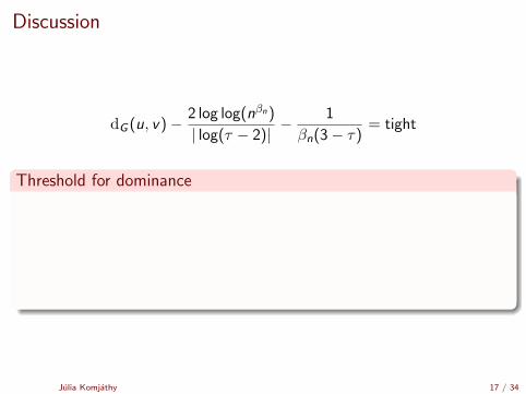
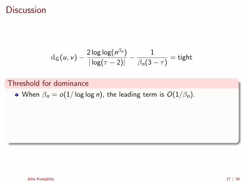
Discussion
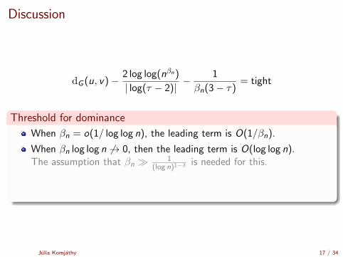
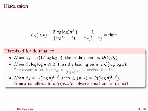
dG (u, v)− 2 log log(nβn)
| log(τ − 2)|− 1
βn(3− τ)= tight
Threshold for dominance
When βn = o(1/ log log n), the leading term is O(1/βn).
When βn log log n 6→ 0, then the leading term is O(log log n).The assumption that βn � 1
(log n)1−δ is needed for this.
When βn = 1/(log n)1−δ, then dG (u, v) = O((log n)1−δ),Truncation allows to interpolate between small and ultrasmall.
Julia Komjathy 17 / 34
Discussion
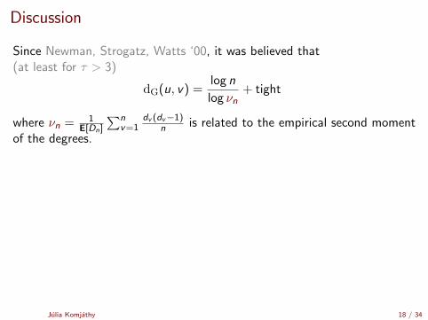
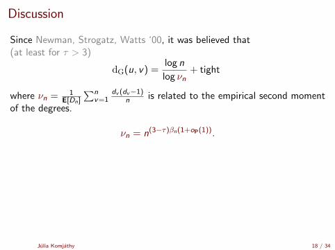
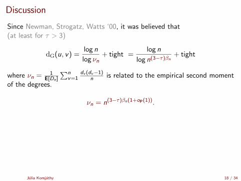
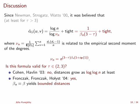
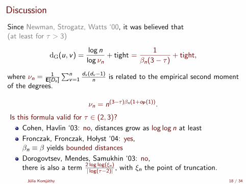
Since Newman, Strogatz, Watts ‘00, it was believed that(at least for τ > 3)
dG(u, v) =log n
log νn+ tight
where νn = 1E[Dn]
∑nv=1
dv (dv−1)n is related to the empirical second moment
of the degrees.
νn = n(3−τ)βn(1+oP(1)).
Is this formula valid for τ ∈ (2, 3)?
Cohen, Havlin ‘03: no, distances grow as log log n at least
Fronczak, Fronczak, Ho lyst ‘04: yes,βn ≡ β yields bounded distances
Dorogovtsev, Mendes, Samukhin ‘03: no,there is also a term 2 log log(ξn)
| log(τ−2)| , with ξn the point of truncation.
Julia Komjathy 18 / 34
Discussion
Since Newman, Strogatz, Watts ‘00, it was believed that(at least for τ > 3)
dG(u, v) =log n
log νn+ tight =
log n
log n(3−τ)βn+ tight
where νn = 1E[Dn]
∑nv=1
dv (dv−1)n is related to the empirical second moment
of the degrees.
νn = n(3−τ)βn(1+oP(1)).
Is this formula valid for τ ∈ (2, 3)?
Cohen, Havlin ‘03: no, distances grow as log log n at least
Fronczak, Fronczak, Ho lyst ‘04: yes,βn ≡ β yields bounded distances
Dorogovtsev, Mendes, Samukhin ‘03: no,there is also a term 2 log log(ξn)
| log(τ−2)| , with ξn the point of truncation.
Julia Komjathy 18 / 34
Discussion
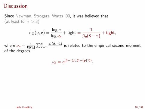
Since Newman, Strogatz, Watts ‘00, it was believed that(at least for τ > 3)
dG(u, v) =log n
log νn+ tight =
1
βn(3− τ)+ tight,
where νn = 1E[Dn]
∑nv=1
dv (dv−1)n is related to the empirical second moment
of the degrees.
νn = n(3−τ)βn(1+oP(1)).
Is this formula valid for τ ∈ (2, 3)?
Cohen, Havlin ‘03: no, distances grow as log log n at least
Fronczak, Fronczak, Ho lyst ‘04: yes,βn ≡ β yields bounded distances
Dorogovtsev, Mendes, Samukhin ‘03: no,there is also a term 2 log log(ξn)
| log(τ−2)| , with ξn the point of truncation.
Julia Komjathy 18 / 34
Discussion
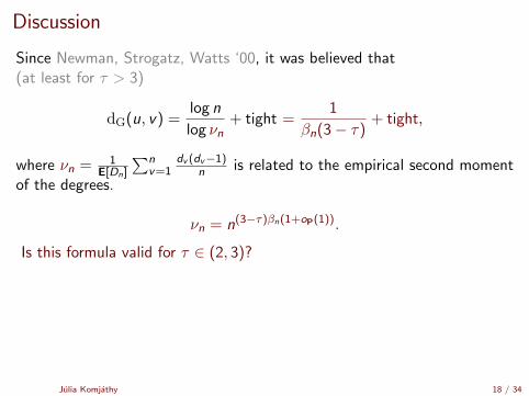
Since Newman, Strogatz, Watts ‘00, it was believed that(at least for τ > 3)
dG(u, v) =log n
log νn+ tight =
1
βn(3− τ)+ tight,
where νn = 1E[Dn]
∑nv=1
dv (dv−1)n is related to the empirical second moment
of the degrees.
νn = n(3−τ)βn(1+oP(1)).
Is this formula valid for τ ∈ (2, 3)?
Cohen, Havlin ‘03: no, distances grow as log log n at least
Fronczak, Fronczak, Ho lyst ‘04: yes,βn ≡ β yields bounded distances
Dorogovtsev, Mendes, Samukhin ‘03: no,there is also a term 2 log log(ξn)
| log(τ−2)| , with ξn the point of truncation.
Julia Komjathy 18 / 34
Discussion
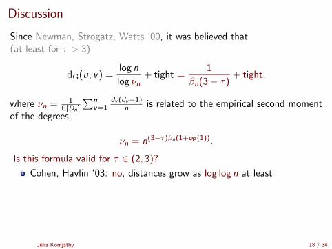
Since Newman, Strogatz, Watts ‘00, it was believed that(at least for τ > 3)
dG(u, v) =log n
log νn+ tight =
1
βn(3− τ)+ tight,
where νn = 1E[Dn]
∑nv=1
dv (dv−1)n is related to the empirical second moment
of the degrees.
νn = n(3−τ)βn(1+oP(1)).
Is this formula valid for τ ∈ (2, 3)?
Cohen, Havlin ‘03: no, distances grow as log log n at least
Fronczak, Fronczak, Ho lyst ‘04: yes,βn ≡ β yields bounded distances
Dorogovtsev, Mendes, Samukhin ‘03: no,there is also a term 2 log log(ξn)
| log(τ−2)| , with ξn the point of truncation.
Julia Komjathy 18 / 34
Discussion
Since Newman, Strogatz, Watts ‘00, it was believed that(at least for τ > 3)
dG(u, v) =log n
log νn+ tight =
1
βn(3− τ)+ tight,
where νn = 1E[Dn]
∑nv=1
dv (dv−1)n is related to the empirical second moment
of the degrees.
νn = n(3−τ)βn(1+oP(1)).
Is this formula valid for τ ∈ (2, 3)?
Cohen, Havlin ‘03: no, distances grow as log log n at least
Fronczak, Fronczak, Ho lyst ‘04: yes,βn ≡ β yields bounded distances
Dorogovtsev, Mendes, Samukhin ‘03: no,there is also a term 2 log log(ξn)
| log(τ−2)| , with ξn the point of truncation.
Julia Komjathy 18 / 34

Proof idea
Julia Komjathy 19 / 34

Distance between hubs
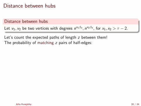
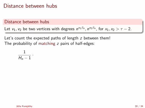
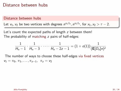
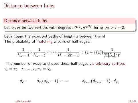
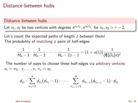
Distance between hubs
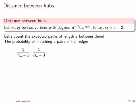
Let v1, v2 be two vertices with degrees nx1βn , nx2βn , for x1, x2 > τ − 2.
Let’s count the expected paths of length z between them!
The probability of matching z pairs of half-edges:
1
Hn − 1· 1
Hn − 3· · · · · 1
Hn − 2z − 1= (1 + o(1))
1
(E[Dn]n)z
The number of ways to choose these half-edges via verticesv1 = π0, πz = v2
dv1 ·
n∑π1=1
dπ1(dπ1 − 1) · · · · ·
n∑πz−1=1
dπz−1(dπz−1 − 1) · dv2
Julia Komjathy 20 / 34
Distance between hubs
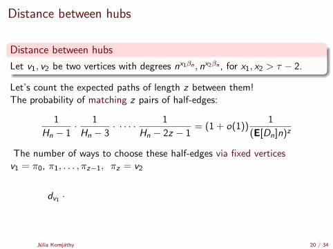
Distance between hubs
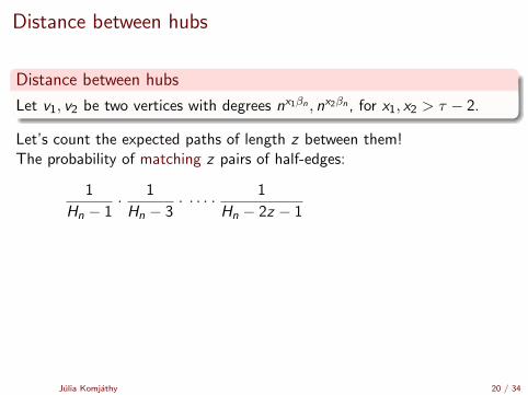
Let v1, v2 be two vertices with degrees nx1βn , nx2βn , for x1, x2 > τ − 2.
Let’s count the expected paths of length z between them!The probability of matching z pairs of half-edges:
1
Hn − 1· 1
Hn − 3· · · · · 1
Hn − 2z − 1= (1 + o(1))
1
(E[Dn]n)z
The number of ways to choose these half-edges via verticesv1 = π0, πz = v2
dv1 ·
n∑π1=1
dπ1(dπ1 − 1) · · · · ·
n∑πz−1=1
dπz−1(dπz−1 − 1) · dv2
Julia Komjathy 20 / 34
Distance between hubs
Distance between hubs
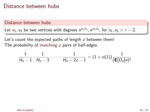
Let v1, v2 be two vertices with degrees nx1βn , nx2βn , for x1, x2 > τ − 2.
Let’s count the expected paths of length z between them!The probability of matching z pairs of half-edges:
1
Hn − 1·
1
Hn − 3· · · · · 1
Hn − 2z − 1= (1 + o(1))
1
(E[Dn]n)z
The number of ways to choose these half-edges via verticesv1 = π0, πz = v2
dv1 ·
n∑π1=1
dπ1(dπ1 − 1) · · · · ·
n∑πz−1=1
dπz−1(dπz−1 − 1) · dv2
Julia Komjathy 20 / 34
Distance between hubs
Distance between hubs
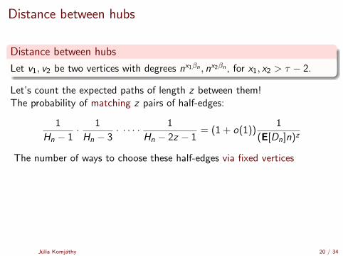
Let v1, v2 be two vertices with degrees nx1βn , nx2βn , for x1, x2 > τ − 2.
Let’s count the expected paths of length z between them!The probability of matching z pairs of half-edges:
1
Hn − 1· 1
Hn − 3·
· · · · 1
Hn − 2z − 1= (1 + o(1))
1
(E[Dn]n)z
The number of ways to choose these half-edges via verticesv1 = π0, πz = v2
dv1 ·
n∑π1=1
dπ1(dπ1 − 1) · · · · ·
n∑πz−1=1
dπz−1(dπz−1 − 1) · dv2
Julia Komjathy 20 / 34
Distance between hubs
Distance between hubs
Let v1, v2 be two vertices with degrees nx1βn , nx2βn , for x1, x2 > τ − 2.
Let’s count the expected paths of length z between them!The probability of matching z pairs of half-edges:
1
Hn − 1· 1
Hn − 3· · · · · 1
Hn − 2z − 1
= (1 + o(1))1
(E[Dn]n)z
The number of ways to choose these half-edges via verticesv1 = π0, πz = v2
dv1 ·
n∑π1=1
dπ1(dπ1 − 1) · · · · ·
n∑πz−1=1
dπz−1(dπz−1 − 1) · dv2
Julia Komjathy 20 / 34
Distance between hubs
Distance between hubs
Let v1, v2 be two vertices with degrees nx1βn , nx2βn , for x1, x2 > τ − 2.
Let’s count the expected paths of length z between them!The probability of matching z pairs of half-edges:
1
Hn − 1· 1
Hn − 3· · · · · 1
Hn − 2z − 1= (1 + o(1))
1
(E[Dn]n)z
The number of ways to choose these half-edges via verticesv1 = π0, πz = v2
dv1 ·
n∑π1=1
dπ1(dπ1 − 1) · · · · ·
n∑πz−1=1
dπz−1(dπz−1 − 1) · dv2
Julia Komjathy 20 / 34
Distance between hubs
Distance between hubs
Let v1, v2 be two vertices with degrees nx1βn , nx2βn , for x1, x2 > τ − 2.
Let’s count the expected paths of length z between them!The probability of matching z pairs of half-edges:
1
Hn − 1· 1
Hn − 3· · · · · 1
Hn − 2z − 1= (1 + o(1))
1
(E[Dn]n)z
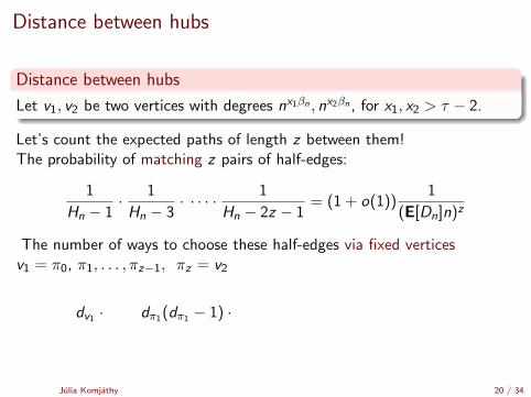
The number of ways to choose these half-edges via fixed vertices
v1 = π0, πz = v2
dv1 ·
n∑π1=1
dπ1(dπ1 − 1) · · · · ·
n∑πz−1=1
dπz−1(dπz−1 − 1) · dv2
Julia Komjathy 20 / 34
Distance between hubs
Distance between hubs
Let v1, v2 be two vertices with degrees nx1βn , nx2βn , for x1, x2 > τ − 2.
Let’s count the expected paths of length z between them!The probability of matching z pairs of half-edges:
1
Hn − 1· 1
Hn − 3· · · · · 1
Hn − 2z − 1= (1 + o(1))
1
(E[Dn]n)z
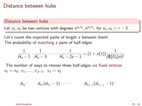
The number of ways to choose these half-edges via fixed verticesv1 = π0, π1, . . . , πz−1, πz = v2
dv1 ·
n∑π1=1
dπ1(dπ1 − 1) · · · · ·
n∑πz−1=1
dπz−1(dπz−1 − 1) · dv2
Julia Komjathy 20 / 34
Distance between hubs
Distance between hubs
Let v1, v2 be two vertices with degrees nx1βn , nx2βn , for x1, x2 > τ − 2.
Let’s count the expected paths of length z between them!The probability of matching z pairs of half-edges:
1
Hn − 1· 1
Hn − 3· · · · · 1
Hn − 2z − 1= (1 + o(1))
1
(E[Dn]n)z
The number of ways to choose these half-edges via fixed verticesv1 = π0, π1, . . . , πz−1, πz = v2
dv1 ·
n∑π1=1
dπ1(dπ1 − 1) ·
· · · ·
n∑πz−1=1
dπz−1(dπz−1 − 1) · dv2
Julia Komjathy 20 / 34
Distance between hubs
Distance between hubs
Let v1, v2 be two vertices with degrees nx1βn , nx2βn , for x1, x2 > τ − 2.
Let’s count the expected paths of length z between them!The probability of matching z pairs of half-edges:
1
Hn − 1· 1
Hn − 3· · · · · 1
Hn − 2z − 1= (1 + o(1))
1
(E[Dn]n)z
The number of ways to choose these half-edges via fixed verticesv1 = π0, π1, . . . , πz−1, πz = v2
dv1 ·
n∑π1=1
dπ1(dπ1 − 1) · · · · ·
n∑πz−1=1
dπz−1(dπz−1 − 1) ·
dv2
Julia Komjathy 20 / 34

Distance between hubs
Distance between hubs
Let v1, v2 be two vertices with degrees nx1βn , nx2βn , for x1, x2 > τ − 2.
Let’s count the expected paths of length z between them!The probability of matching z pairs of half-edges:
1
Hn − 1· 1
Hn − 3· · · · · 1
Hn − 2z − 1= (1 + o(1))
1
(E[Dn]n)z
The number of ways to choose these half-edges via fixed verticesv1 = π0, π1, . . . , πz−1, πz = v2
dv1 ·
n∑π1=1
dπ1(dπ1 − 1) · · · · ·
n∑πz−1=1
dπz−1(dπz−1 − 1) · dv2
Julia Komjathy 20 / 34
Distance between hubs
Distance between hubs
Let v1, v2 be two vertices with degrees nx1βn , nx2βn , for x1, x2 > τ − 2.
Let’s count the expected paths of length z between them!The probability of matching z pairs of half-edges:
1
Hn − 1· 1
Hn − 3· · · · · 1
Hn − 2z − 1= (1 + o(1))
1
(E[Dn]n)z
The number of ways to choose these half-edges via arbitrary verticesv1 = π0, ?, . . . , ?, πz = v2
dv1 ·n∑
π1=1
dπ1(dπ1 − 1) · · · · ·n∑
πz−1=1
dπz−1(dπz−1 − 1) · dv2
Julia Komjathy 20 / 34
Distance between hubs
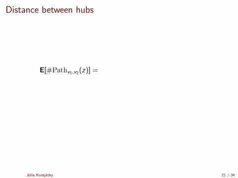
E[#Pathv1,v2(z)] =
(1 + o(1))1 · dv1 ·
(n∑
v=1
)z−1
dv2
= C · 1
n· dv1 · dv2 · n(z−1)(3−τ)βn
= C · 1
n· nx1βn · nx2βn · n(z−1)(3−τ)βn
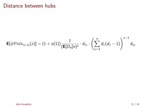
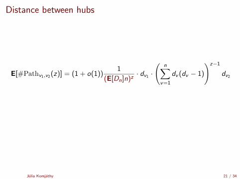
What is the smallest z so that this does not tend to 0?
Julia Komjathy 21 / 34
Distance between hubs
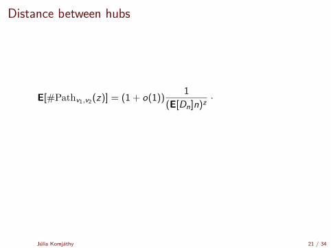
E[#Pathv1,v2(z)] = (1 + o(1))1
(E[Dn]n)z·
dv1 ·
(n∑
v=1
)z−1
dv2
= C · 1
n· dv1 · dv2 · n(z−1)(3−τ)βn
= C · 1
n· nx1βn · nx2βn · n(z−1)(3−τ)βn
What is the smallest z so that this does not tend to 0?
Julia Komjathy 21 / 34
Distance between hubs
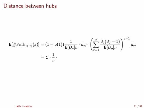
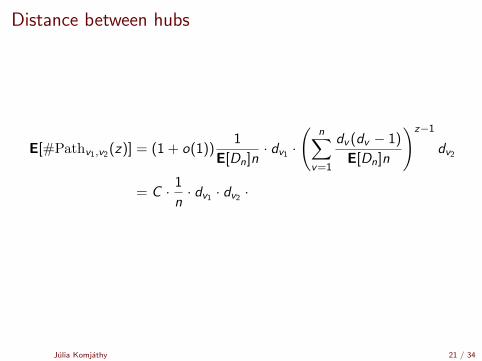
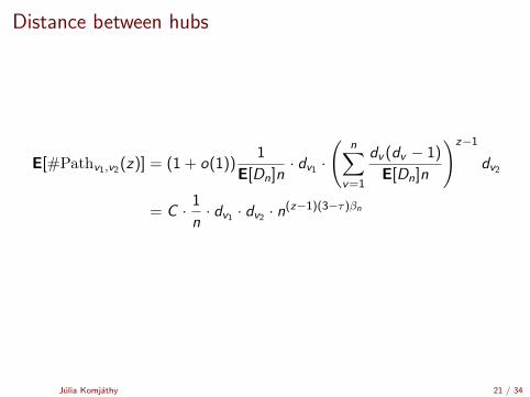
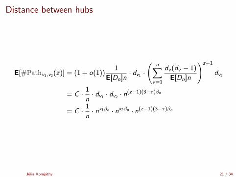
E[#Pathv1,v2(z)] = (1 + o(1))1
(E[Dn]n)z· dv1 ·
(n∑
v=1
dv (dv − 1)
)z−1
dv2
= C · 1
n· dv1 · dv2 · n(z−1)(3−τ)βn
= C · 1
n· nx1βn · nx2βn · n(z−1)(3−τ)βn
What is the smallest z so that this does not tend to 0?
Julia Komjathy 21 / 34
Distance between hubs
E[#Pathv1,v2(z)] = (1 + o(1))1
(E[Dn]n)z· dv1 ·
(n∑
v=1
dv (dv − 1)
)z−1
dv2
= C · 1
n· dv1 · dv2 · n(z−1)(3−τ)βn
= C · 1
n· nx1βn · nx2βn · n(z−1)(3−τ)βn
What is the smallest z so that this does not tend to 0?
Julia Komjathy 21 / 34
Distance between hubs
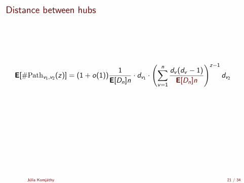
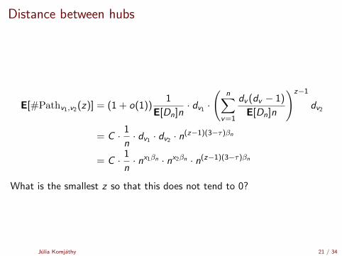
E[#Pathv1,v2(z)] = (1 + o(1))1
E[Dn]n· dv1 ·
(n∑
v=1
dv (dv − 1)
E[Dn]n
)z−1
dv2
= C · 1
n· dv1 · dv2 · n(z−1)(3−τ)βn
= C · 1
n· nx1βn · nx2βn · n(z−1)(3−τ)βn
What is the smallest z so that this does not tend to 0?
Julia Komjathy 21 / 34
Distance between hubs
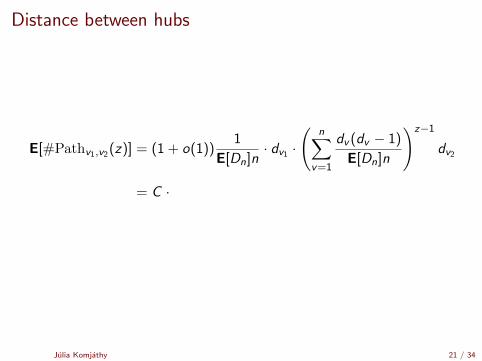
E[#Pathv1,v2(z)] = (1 + o(1))1
E[Dn]n· dv1 ·
(n∑
v=1
dv (dv − 1)
E[Dn]n
)z−1
dv2
= C ·
1
n· dv1 · dv2 · n(z−1)(3−τ)βn
= C · 1
n· nx1βn · nx2βn · n(z−1)(3−τ)βn
What is the smallest z so that this does not tend to 0?
Julia Komjathy 21 / 34
Distance between hubs
E[#Pathv1,v2(z)] = (1 + o(1))1
E[Dn]n· dv1 ·
(n∑
v=1
dv (dv − 1)
E[Dn]n
)z−1
dv2
= C · 1
n·
dv1 · dv2 · n(z−1)(3−τ)βn
= C · 1
n· nx1βn · nx2βn · n(z−1)(3−τ)βn
What is the smallest z so that this does not tend to 0?
Julia Komjathy 21 / 34
Distance between hubs
E[#Pathv1,v2(z)] = (1 + o(1))1
E[Dn]n· dv1 ·
(n∑
v=1
dv (dv − 1)
E[Dn]n
)z−1
dv2
= C · 1
n· dv1 · dv2 ·
n(z−1)(3−τ)βn
= C · 1
n· nx1βn · nx2βn · n(z−1)(3−τ)βn
What is the smallest z so that this does not tend to 0?
Julia Komjathy 21 / 34
Distance between hubs
E[#Pathv1,v2(z)] = (1 + o(1))1
E[Dn]n· dv1 ·
(n∑
v=1
dv (dv − 1)
E[Dn]n
)z−1
dv2
= C · 1
n· dv1 · dv2 · n(z−1)(3−τ)βn
= C · 1
n· nx1βn · nx2βn · n(z−1)(3−τ)βn
What is the smallest z so that this does not tend to 0?
Julia Komjathy 21 / 34
Distance between hubs
E[#Pathv1,v2(z)] = (1 + o(1))1
E[Dn]n· dv1 ·
(n∑
v=1
dv (dv − 1)
E[Dn]n
)z−1
dv2
= C · 1
n· dv1 · dv2 · n(z−1)(3−τ)βn
= C · 1
n· nx1βn · nx2βn · n(z−1)(3−τ)βn
What is the smallest z so that this does not tend to 0?
Julia Komjathy 21 / 34
Distance between hubs
E[#Pathv1,v2(z)] = (1 + o(1))1
E[Dn]n· dv1 ·
(n∑
v=1
dv (dv − 1)
E[Dn]n
)z−1
dv2
= C · 1
n· dv1 · dv2 · n(z−1)(3−τ)βn
= C · 1
n· nx1βn · nx2βn · n(z−1)(3−τ)βn
What is the smallest z so that this does not tend to 0?
Julia Komjathy 21 / 34
Distance between hubs
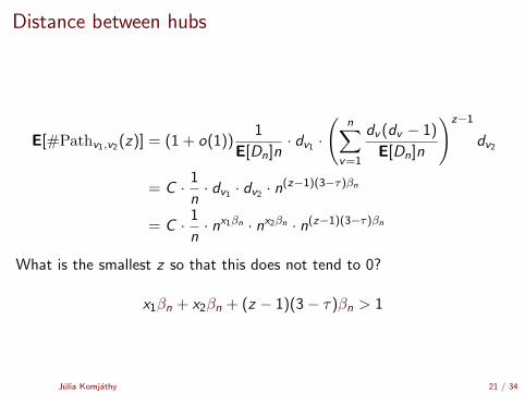
E[#Pathv1,v2(z)] = (1 + o(1))1
E[Dn]n· dv1 ·
(n∑
v=1
dv (dv − 1)
E[Dn]n
)z−1
dv2
= C · 1
n· dv1 · dv2 · n(z−1)(3−τ)βn
= C · 1
n· nx1βn · nx2βn · n(z−1)(3−τ)βn
What is the smallest z so that this does not tend to 0?
x1βn + x2βn + (z − 1)(3− τ)βn > 1
Julia Komjathy 21 / 34
Distance between hubs
E[#Pathv1,v2(z)] = (1 + o(1))1
E[Dn]n· dv1 ·
(n∑
v=1
dv (dv − 1)
E[Dn]n
)z−1
dv2
= C · 1
n· dv1 · dv2 · n(z−1)(3−τ)βn
= C · 1
n· nx1βn · nx2βn · n(z−1)(3−τ)βn
What is the smallest z so that this does not tend to 0?
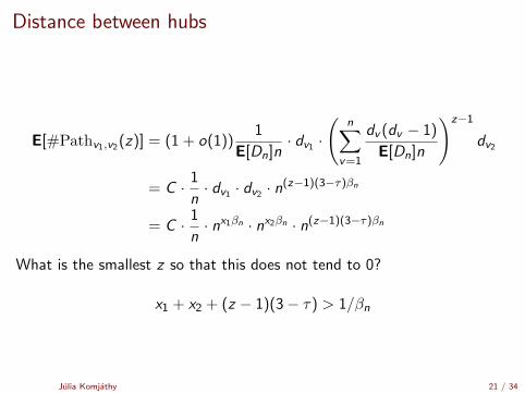
x1 + x2 + (z − 1)(3− τ) > 1/βn
Julia Komjathy 21 / 34

Distance between hubs
E[#Pathv1,v2(z)] = (1 + o(1))1
E[Dn]n· dv1 ·
(n∑
v=1
dv (dv − 1)
E[Dn]n
)z−1
dv2
= C · 1
n· dv1 · dv2 · n(z−1)(3−τ)βn
= C · 1
n· nx1βn · nx2βn · n(z−1)(3−τ)βn
What is the smallest z so that this does not tend to 0?
(z − 1)(3− τ) > 1/βn − x1 − x2
Julia Komjathy 21 / 34
Distance between hubs
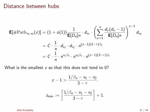
E[#Pathv1,v2(z)] = (1 + o(1))1
E[Dn]n· dv1 ·
(n∑
v=1
dv (dv − 1)
E[Dn]n
)z−1
dv2
= C · 1
n· dv1 · dv2 · n(z−1)(3−τ)βn
= C · 1
n· nx1βn · nx2βn · n(z−1)(3−τ)βn
What is the smallest z so that this does not tend to 0?
z − 1 >1/βn − x1 − x2
3− τ.
zmin :=
⌈1/βn − x1 − x2
3− τ
⌉+ 1.
Julia Komjathy 21 / 34
Distance between hubs
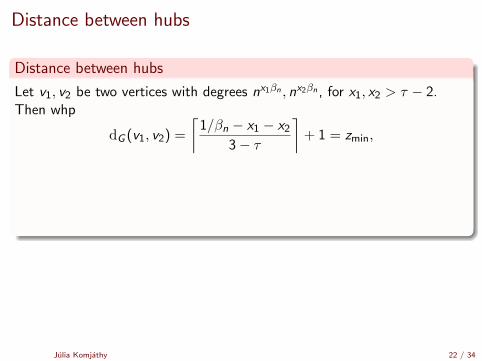
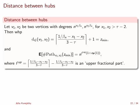
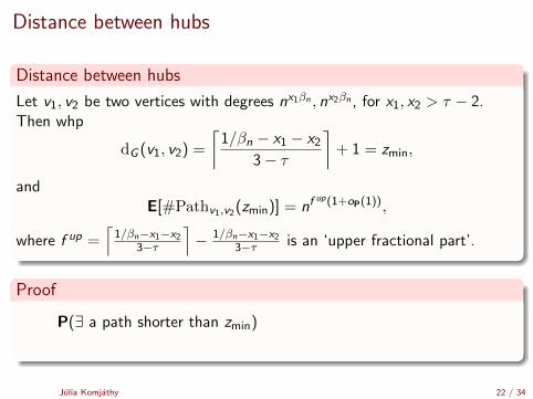
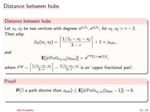
Distance between hubs
Let v1, v2 be two vertices with degrees nx1βn , nx2βn , for x1, x2 > τ − 2.Then whp
dG (v1, v2) =
⌈1/βn − x1 − x2
3− τ
⌉+ 1 = zmin,
andE[#Pathv1,v2(zmin)] = nf
up(1+oP(1)),
where f up =⌈
1/βn−x1−x2
3−τ
⌉− 1/βn−x1−x2
3−τ is an ‘upper fractional part’.
Proof
P(∃ a path shorter than zmin)
≤ E[#Pathv1,v2(zmin − 1)]→ 0.
Julia Komjathy 22 / 34
Distance between hubs
Distance between hubs
Let v1, v2 be two vertices with degrees nx1βn , nx2βn , for x1, x2 > τ − 2.Then whp
dG (v1, v2) =
⌈1/βn − x1 − x2
3− τ
⌉+ 1 = zmin,
andE[#Pathv1,v2(zmin)] = nf
up(1+oP(1)),
where f up =⌈
1/βn−x1−x2
3−τ
⌉− 1/βn−x1−x2
3−τ is an ‘upper fractional part’.
Proof
P(∃ a path shorter than zmin) ≤ E[#Pathv1,v2(zmin − 1)]→ 0.
Julia Komjathy 22 / 34
The other direction
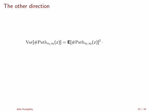
Var[#Pathv1,v2(z)] = E[#Pathv1,v2(z)]2 ·
n(τ−2)βn ·
This tends to zero if and only if min{x1, x2} > τ − 2.
From here, Chebyshev’s inequality finishes the proof.
Julia Komjathy 23 / 34
The other direction
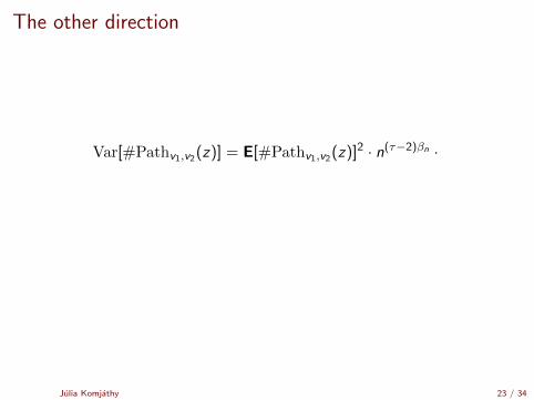
Var[#Pathv1,v2(z)] = E[#Pathv1,v2(z)]2 · n(τ−2)βn ·
This tends to zero if and only if min{x1, x2} > τ − 2.
From here, Chebyshev’s inequality finishes the proof.
Julia Komjathy 23 / 34
The other direction
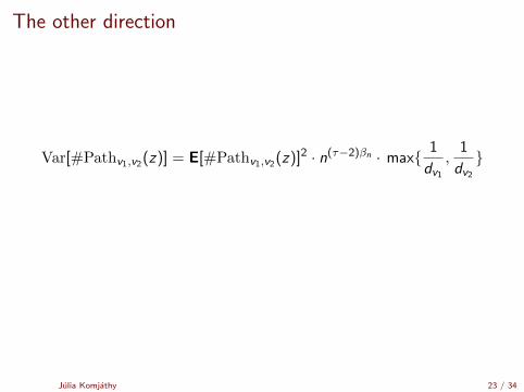
Var[#Pathv1,v2(z)] = E[#Pathv1,v2(z)]2 · n(τ−2)βn · max{ 1
dv1
,1
dv2
}
This tends to zero if and only if min{x1, x2} > τ − 2.
From here, Chebyshev’s inequality finishes the proof.
Julia Komjathy 23 / 34
The other direction
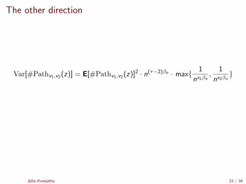
Var[#Pathv1,v2(z)] = E[#Pathv1,v2(z)]2 · n(τ−2)βn · max{ 1
nx1βn,
1
nx2βn}
This tends to zero if and only if min{x1, x2} > τ − 2.
From here, Chebyshev’s inequality finishes the proof.
Julia Komjathy 23 / 34
The other direction
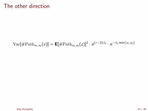
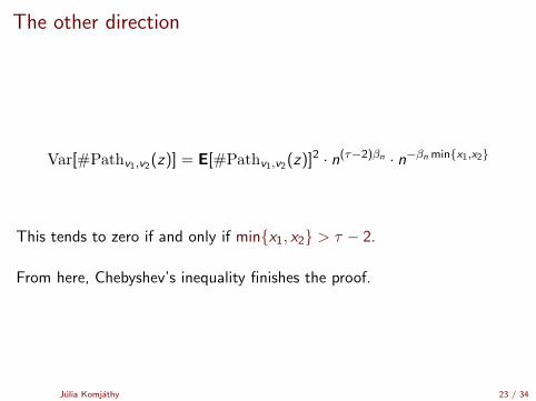
Var[#Pathv1,v2(z)] = E[#Pathv1,v2(z)]2 · n(τ−2)βn · n−βn min{x1,x2}
This tends to zero if and only if min{x1, x2} > τ − 2.
From here, Chebyshev’s inequality finishes the proof.
Julia Komjathy 23 / 34
The other direction
Var[#Pathv1,v2(z)] = E[#Pathv1,v2(z)]2 · n(τ−2)βn · n−βn min{x1,x2}
This tends to zero if and only if min{x1, x2} > τ − 2.
From here, Chebyshev’s inequality finishes the proof.
Julia Komjathy 23 / 34
Comment
Distance between hubs
Let v1, v2 be two vertices with degrees nx1βn , nx2βn , for x1, x2 > τ − 2.Then whp
dG (v1, v2) =
⌈1/βn − x1 − x2
3− τ
⌉+ 1 =
1
βn(3− τ)+ tight,
so the formula from physics is valid only between hubs!
Julia Komjathy 24 / 34
Comment
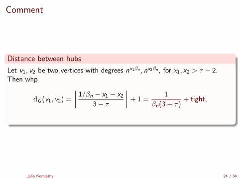
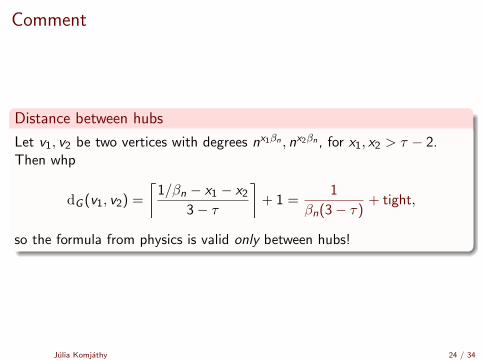
Distance between hubs
Let v1, v2 be two vertices with degrees nx1βn , nx2βn , for x1, x2 > τ − 2.Then whp
dG (v1, v2) =
⌈1/βn − x1 − x2
3− τ
⌉+ 1 =
1
βn(3− τ)+ tight,
so the formula from physics is valid only between hubs!
Julia Komjathy 24 / 34

How to get to the hubs?
When constructing the shortest path, how long does it take to get to thehubs?
Julia Komjathy 25 / 34

Neighborhood growth
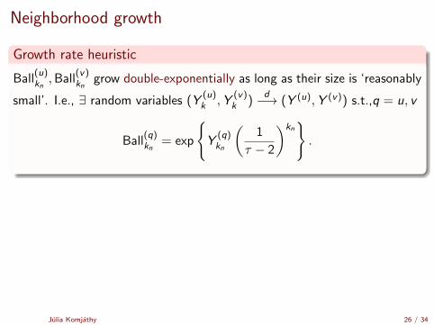
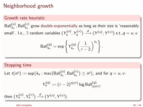
Growth rate heuristic
Ball(u)kn,Ball
(v)kn
grow double-exponentially as long as their size is ‘reasonably
small’.
I.e., ∃ random variables (Y(u)k ,Y
(v)k )
d−→ (Y (u),Y (v)) s.t.,q = u, v
Ball(q)kn
= exp
{Y
(q)kn
(1
τ − 2
)kn}.
Stopping time
Let t(n%) := sup{kn : max{Ball(u)kn,Ball
(v)kn} ≤ n%}, and for q = u, v :
Y(q)n := (τ − 2)t(n%) log Ball
(q)t(n%),
then (Y(u)n ,Y
(v)n )
d−→ (Y (u),Y (v)).
Julia Komjathy 26 / 34

Neighborhood growth
Growth rate heuristic
Ball(u)kn,Ball
(v)kn
grow double-exponentially as long as their size is ‘reasonably
small’.
I.e., ∃ random variables (Y(u)k ,Y
(v)k )
d−→ (Y (u),Y (v)) s.t.,q = u, v
Ball(q)kn
= exp
{Y
(q)kn
(1
τ − 2
)kn}.
Stopping time
Let t(n%) := sup{kn : max{Ball(u)kn,Ball
(v)kn} ≤ n%}, and for q = u, v :
Y(q)n := (τ − 2)t(n%) log Ball
(q)t(n%),
then (Y(u)n ,Y
(v)n )
d−→ (Y (u),Y (v)).
Julia Komjathy 26 / 34
Neighborhood growth
Growth rate heuristic
Ball(u)kn,Ball
(v)kn
grow double-exponentially as long as their size is ‘reasonably
small’. I.e., ∃ random variables (Y(u)k ,Y
(v)k )
d−→ (Y (u),Y (v)) s.t.,q = u, v
Ball(q)kn
= exp
{Y
(q)kn
(1
τ − 2
)kn}.
Stopping time
Let t(n%) := sup{kn : max{Ball(u)kn,Ball
(v)kn} ≤ n%}, and for q = u, v :
Y(q)n := (τ − 2)t(n%) log Ball
(q)t(n%),
then (Y(u)n ,Y
(v)n )
d−→ (Y (u),Y (v)).
Julia Komjathy 26 / 34
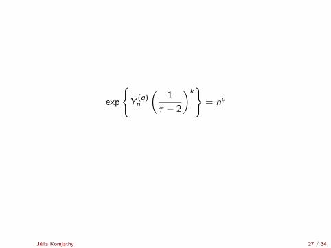
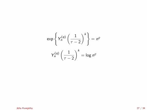
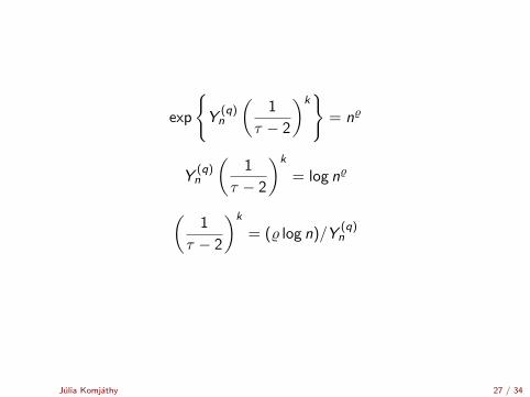
exp
{Y
(q)n
(1
τ − 2
)k}
= n%
Julia Komjathy 27 / 34
exp
{Y
(q)n
(1
τ − 2
)k}
= n%
Y(q)n
(1
τ − 2
)k
= log n%
Julia Komjathy 27 / 34
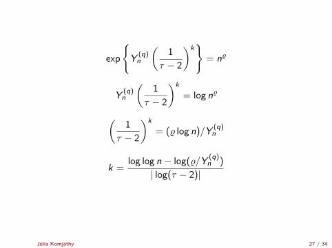
exp
{Y
(q)n
(1
τ − 2
)k}
= n%
Y(q)n
(1
τ − 2
)k
= log n%
(1
τ − 2
)k
= (% log n)/Y(q)n
Julia Komjathy 27 / 34
exp
{Y
(q)n
(1
τ − 2
)k}
= n%
Y(q)n
(1
τ − 2
)k
= log n%
(1
τ − 2
)k
= (% log n)/Y(q)n
k =log log n − log(%/Y
(q)n )
| log(τ − 2)|
Julia Komjathy 27 / 34
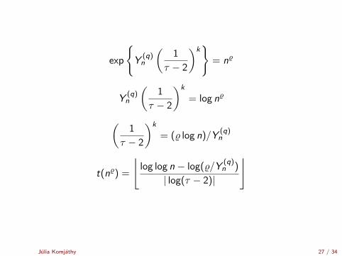
exp
{Y
(q)n
(1
τ − 2
)k}
= n%
Y(q)n
(1
τ − 2
)k
= log n%
(1
τ − 2
)k
= (% log n)/Y(q)n
t(n%) =
⌊log log n − log(%/Y
(q)n )
| log(τ − 2)|
⌋
Julia Komjathy 27 / 34

Shell structure
Step 1
One can find a vertex of degree ≈ Ball(q)t(n%) in the balls.
Step 2
Structure the high-degree part of the graph in layers of roughly equaldegree (on a log log scale).
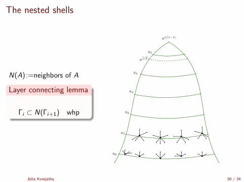
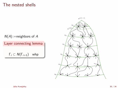
Shell i :
Γi = {v : dv ≥ n%(τ−2)−i(1 + o(1))}
Like shells of an onion, to get to the core of the graph.
Julia Komjathy 28 / 34

Shell structure
Step 1
One can find a vertex of degree ≈ Ball(q)t(n%) in the balls.
Step 2
Structure the high-degree part of the graph in layers of roughly equaldegree (on a log log scale).
Shell i :
Γi = {v : dv ≥ n%(τ−2)−i(1 + o(1))}
Like shells of an onion, to get to the core of the graph.
Julia Komjathy 28 / 34
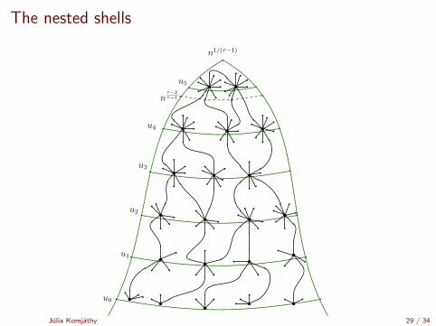
The nested shells
j j
n1/(τ−1)
u0
u1
u2
u3
u4
u5
nτ−2τ−1
Julia Komjathy 29 / 34
The nested shells
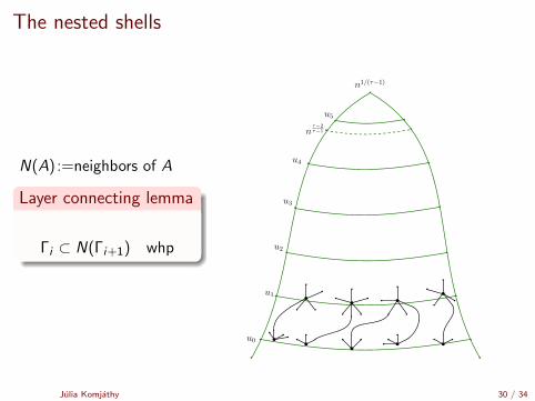
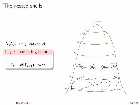
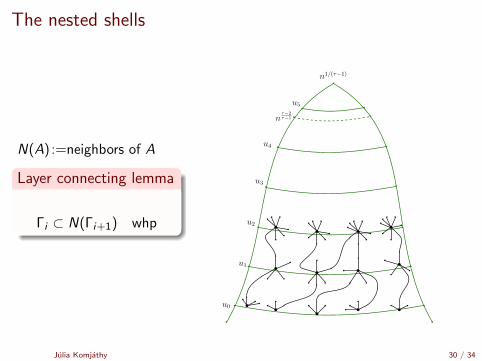
N(A) :=neighbors of A
Layer connecting lemma
Γi ⊂ N(Γi+1) whp
j j
n1/(τ−1)
u0
u1
u2
u3
u4
u5
nτ−2τ−1
Julia Komjathy 30 / 34
The nested shells
N(A) :=neighbors of A
Layer connecting lemma
Γi ⊂ N(Γi+1) whp
j j
n1/(τ−1)
u0
u1
u2
u3
u4
u5
nτ−2τ−1
Julia Komjathy 30 / 34
The nested shells
N(A) :=neighbors of A
Layer connecting lemma
Γi ⊂ N(Γi+1) whp
j j
n1/(τ−1)
u0
u1
u2
u3
u4
u5
nτ−2τ−1
Julia Komjathy 30 / 34
The nested shells
N(A) :=neighbors of A
Layer connecting lemma
Γi ⊂ N(Γi+1) whp
j j
n1/(τ−1)
u0
u1
u2
u3
u4
u5
nτ−2τ−1
Julia Komjathy 30 / 34
The nested shells
N(A) :=neighbors of A
Layer connecting lemma
Γi ⊂ N(Γi+1) whp
j j
n1/(τ−1)
u0
u1
u2
u3
u4
u5
nτ−2τ−1
Julia Komjathy 30 / 34
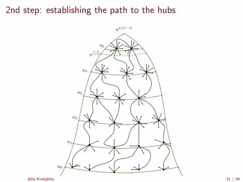
2nd step: establishing the path to the hubs
j j
n1/(τ−1)
u0
u1
u2
u3
u4
u5
nτ−2τ−1
Julia Komjathy 31 / 34
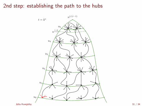
2nd step: establishing the path to the hubs
t = k?
j j
n1/(τ−1)
u0
u1
u2
u3
u4
u5
nτ−2τ−1
Julia Komjathy 31 / 34
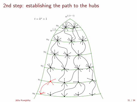
2nd step: establishing the path to the hubs
t = k? + 1
j j
n1/(τ−1)
u0
u1
u2
u3
u4
u5
nτ−2τ−1
Julia Komjathy 31 / 34
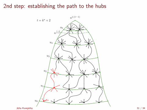
2nd step: establishing the path to the hubs
t = k? + 2
j j
n1/(τ−1)
u0
u1
u2
u3
u4
u5
nτ−2τ−1
Julia Komjathy 31 / 34
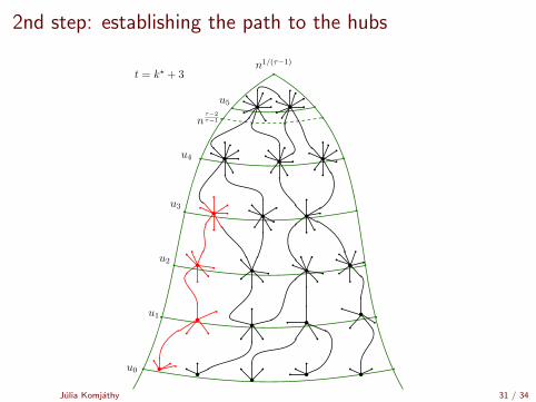
2nd step: establishing the path to the hubs
t = k? + 3
j j
n1/(τ−1)
u0
u1
u2
u3
u4
u5
nτ−2τ−1
Julia Komjathy 31 / 34
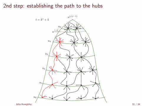
2nd step: establishing the path to the hubs
t = k? + 4
j j
n1/(τ−1)
u0
u1
u2
u3
u4
u5
nτ−2τ−1
Julia Komjathy 31 / 34
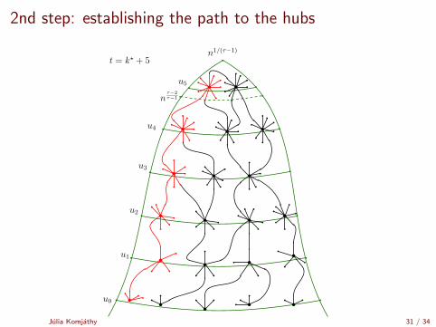
2nd step: establishing the path to the hubs
t = k? + 5
j j
n1/(τ−1)
u0
u1
u2
u3
u4
u5
nτ−2τ−1
Julia Komjathy 31 / 34
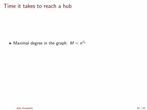
Time it takes to reach a hub
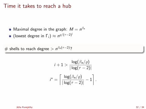
Maximal degree in the graph: M = nβn
(lowest degree in Γi ) ≈ n%/(τ−2)i
# shells to reach degree > nβn(τ−2)?
Julia Komjathy 32 / 34
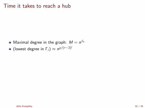
Time it takes to reach a hub
Maximal degree in the graph: M = nβn
(lowest degree in Γi ) ≈ n%/(τ−2)i
# shells to reach degree > nβn(τ−2)?
Julia Komjathy 32 / 34

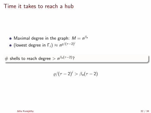
Time it takes to reach a hub
Maximal degree in the graph: M = nβn
(lowest degree in Γi ) ≈ n%/(τ−2)i
# shells to reach degree > nβn(τ−2)?
Julia Komjathy 32 / 34

Time it takes to reach a hub
Maximal degree in the graph: M = nβn
(lowest degree in Γi ) ≈ n%/(τ−2)i
# shells to reach degree > nβn(τ−2)?
n%/(τ−2)i > nβn(τ−2)
Julia Komjathy 32 / 34
Time it takes to reach a hub
Maximal degree in the graph: M = nβn
(lowest degree in Γi ) ≈ n%/(τ−2)i
# shells to reach degree > nβn(τ−2)?
%/(τ − 2)i > βn(τ − 2)
Julia Komjathy 32 / 34

Time it takes to reach a hub
Maximal degree in the graph: M = nβn
(lowest degree in Γi ) ≈ n%/(τ−2)i
# shells to reach degree > nβn(τ−2)?
1/(τ − 2)i+1 > βn/%
Julia Komjathy 32 / 34
Time it takes to reach a hub
Maximal degree in the graph: M = nβn
(lowest degree in Γi ) ≈ n%/(τ−2)i
# shells to reach degree > nβn(τ−2)?
i + 1 >log(βn/%)
| log(τ − 2)|
Julia Komjathy 32 / 34
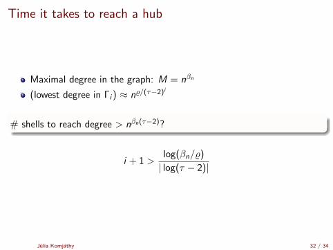
Time it takes to reach a hub
Maximal degree in the graph: M = nβn
(lowest degree in Γi ) ≈ n%/(τ−2)i
# shells to reach degree > nβn(τ−2)?
i + 1 >log(βn/%)
| log(τ − 2)|
i? =
⌈log(βn/%)
| log(τ − 2)|− 1
⌉.
Julia Komjathy 32 / 34

Time to reach the top
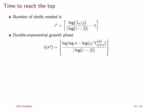
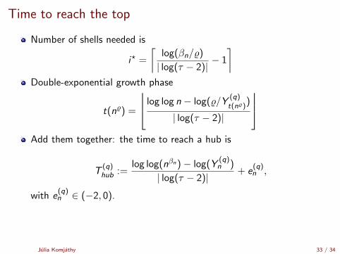
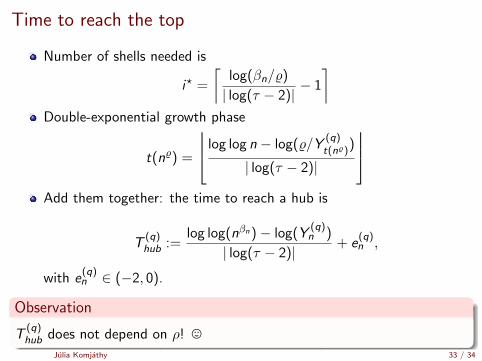
Number of shells needed is
i? =
⌈log(βn/%)
| log(τ − 2)|− 1
⌉
Double-exponential growth phase
t(n%) =
log log n − log(%/Y(q)t(n%))
| log(τ − 2)|
Add them together: the time to reach a hub is
T(q)hub :=
log log(nβn)− log(Y(q)n )
| log(τ − 2)|+ e
(q)n ,
with e(q)n ∈ (−2, 0).
Observation
T(q)hub does not depend on ρ! ,
Julia Komjathy 33 / 34
Time to reach the top
Number of shells needed is
i? =
⌈log(βn/%)
| log(τ − 2)|− 1
⌉Double-exponential growth phase
t(n%) =
log log n − log(%/Y(q)t(n%))
| log(τ − 2)|
Add them together: the time to reach a hub is
T(q)hub :=
log log(nβn)− log(Y(q)n )
| log(τ − 2)|+ e
(q)n ,
with e(q)n ∈ (−2, 0).
Observation
T(q)hub does not depend on ρ! ,
Julia Komjathy 33 / 34
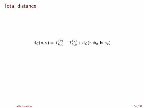
Total distance
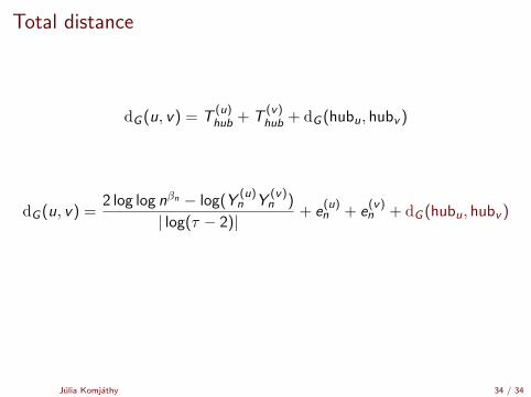
dG (u, v) = T(u)hub + T
(v)hub + dG (hubu, hubv )
,,,
Julia Komjathy 34 / 34
Total distance
dG (u, v) = T(u)hub + T
(v)hub + dG (hubu, hubv )
,,,
Julia Komjathy 34 / 34
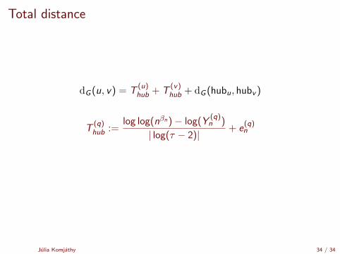
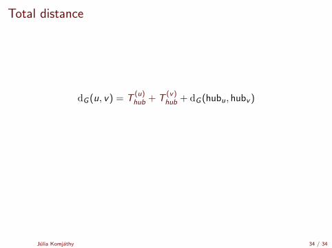
Total distance
dG (u, v) = T(u)hub + T
(v)hub + dG (hubu, hubv )
T(q)hub :=
log log(nβn)− log(Y(q)n )
| log(τ − 2)|+ e
(q)n
,,,
Julia Komjathy 34 / 34
Total distance
dG (u, v) = T(u)hub + T
(v)hub + dG (hubu, hubv )
T(q)hub :=
log log(nβn)− log(Y(q)n )
| log(τ − 2)|+ e
(q)n
dG (u, v) =2 log log nβn − log(Y
(u)n Y
(v)n )
| log(τ − 2)|+ e
(u)n + e
(v)n + dG (hubu, hubv )
,,,
Julia Komjathy 34 / 34
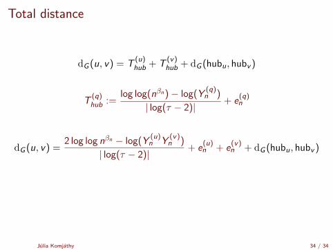
Total distance
dG (u, v) = T(u)hub + T
(v)hub + dG (hubu, hubv )
dG (u, v) =2 log log nβn − log(Y
(u)n Y
(v)n )
| log(τ − 2)|+ e
(u)n + e
(v)n + dG (hubu, hubv )
,,,
Julia Komjathy 34 / 34
Total distance
dG (u, v) = T(u)hub + T
(v)hub + dG (hubu, hubv )
dG (u, v) =2 log log nβn − log(Y
(u)n Y
(v)n )
| log(τ − 2)|+ e
(u)n + e
(v)n + dG (hubu, hubv )
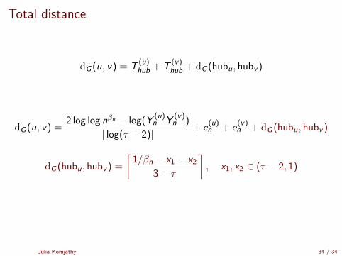
dG (hubu, hubv ) =
⌈1/βn − x1 − x2
3− τ
⌉, x1, x2 ∈ (τ − 2, 1)
,,,
Julia Komjathy 34 / 34
Total distance
dG (u, v) = T(u)hub + T
(v)hub + dG (hubu, hubv )
dG (u, v) =2 log log nβn − log(Y
(u)n Y
(v)n )
| log(τ − 2)|+ e
(u)n + e
(v)n
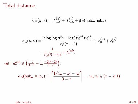
+1
βn(3− τ)+ ehubn ,
with ehubn ∈(−2
3−τ − 1, −2(τ−2)3−τ
).
dG (hubu, hubv ) =
⌈1/βn − x1 − x2
3− τ
⌉, x1, x2 ∈ (τ − 2, 1)
,,,
Julia Komjathy 34 / 34
Total distance
dG (u, v) = T(u)hub + T
(v)hub + dG (hubu, hubv )
dG (u, v) =2 log log nβn − log(Y
(u)n Y
(v)n )
| log(τ − 2)|
+1
βn(3− τ)
+ tight.
,,,
Julia Komjathy 34 / 34
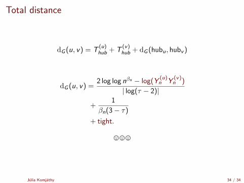
Total distance
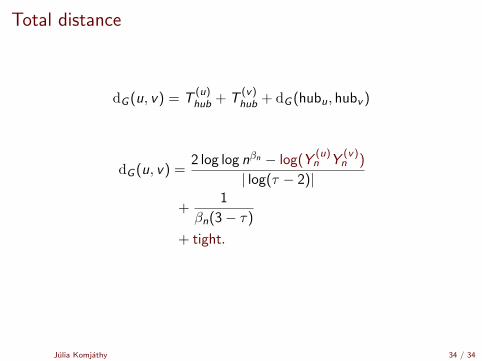
dG (u, v) = T(u)hub + T
(v)hub + dG (hubu, hubv )
dG (u, v) =2 log log nβn − log(Y
(u)n Y
(v)n )
| log(τ − 2)|
+1
βn(3− τ)
+ tight.
,,,
Julia Komjathy 34 / 34

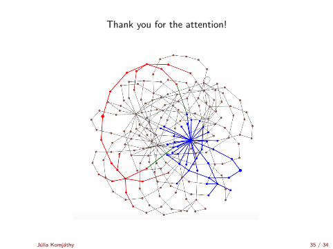
Thank you for the attention!
Julia Komjathy 35 / 34
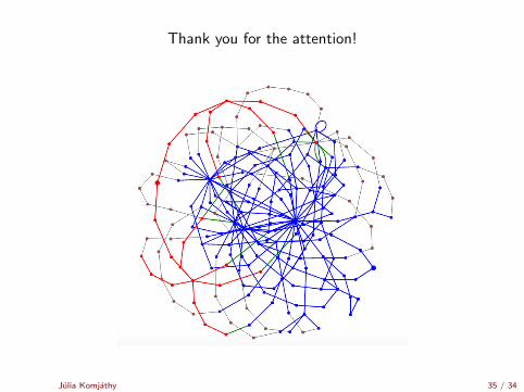
Thank you for the attention!
Julia Komjathy 35 / 34
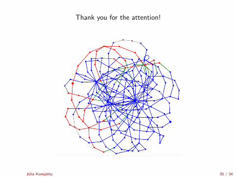
Thank you for the attention!
Julia Komjathy 35 / 34
Thank you for the attention!
Julia Komjathy 35 / 34