What’s

Your

Function?

Convolution jct.

Jeff Swanson

John Rivera

Ben Rougier

Justin Malaise

Craig Rykal

The Team:

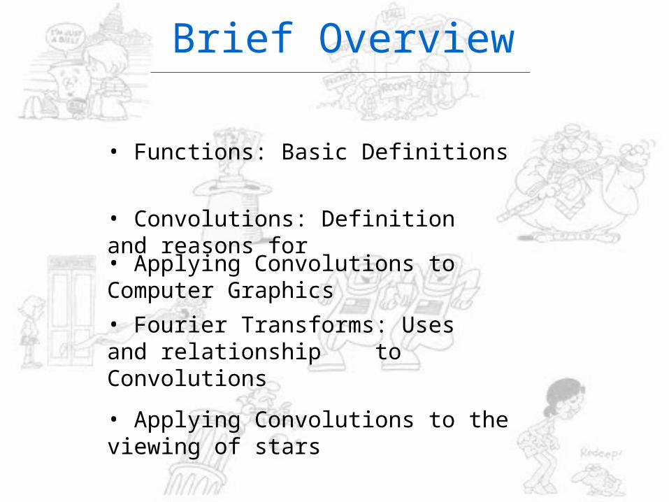
Brief Overview

• Functions: Basic Definitions

• Fourier Transforms: Uses and relationship to Convolutions

• Convolutions: Definition and reasons for

• Applying Convolutions to Computer Graphics

• Applying Convolutions to the viewing of stars

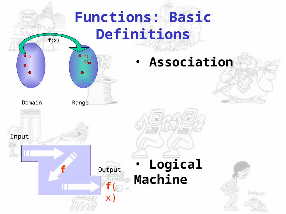
x

Input

Domain Range

f(x)

x f(x) • Association

f • Logical Machine

f(x)

Output

Functions: Basic Definitions

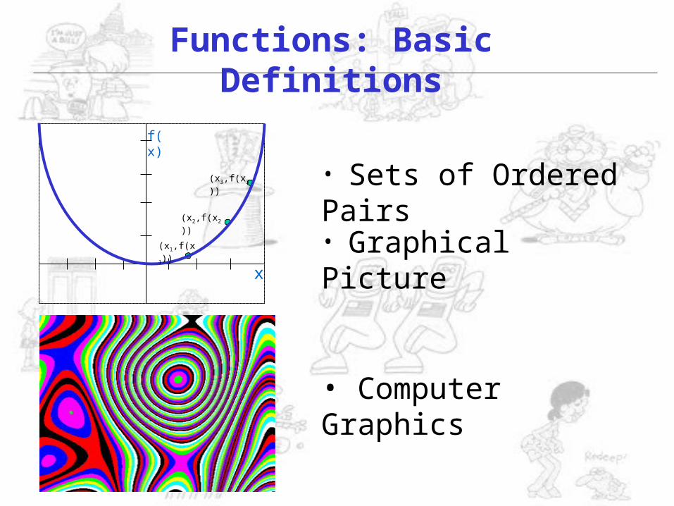
(x1,f(x1))

(x2,f(x2))

(x3,f(x3))

• Graphical Picture

• Sets of Ordered Pairs

f(x)

x

Functions: Basic Definitions

• Computer Graphics

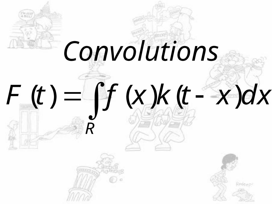
Convolutions

R

dxxtkxftF )()()(

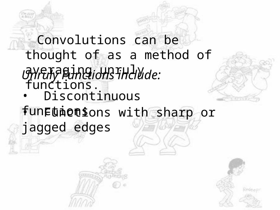
Convolutions can be thought of as a method of averaging unruly functions.

Unruly Functions include:

• Discontinuous functions• Functions with sharp or jagged edges

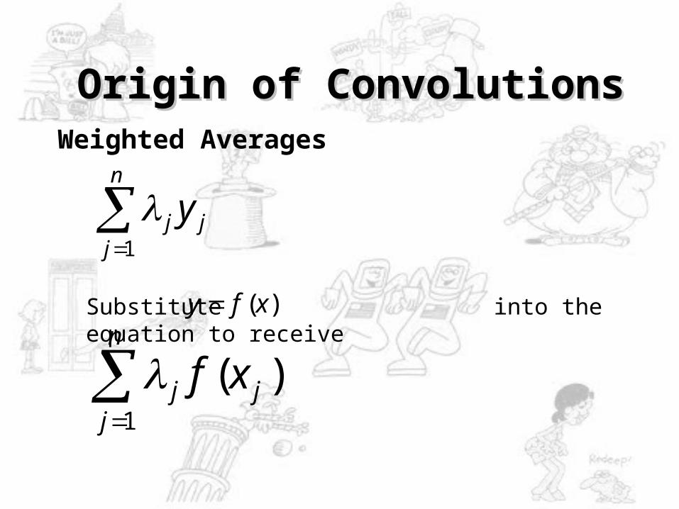
Weighted Averages

n

jjj y

1

Origin of ConvolutionsOrigin of Convolutions

Substitute into the equation to receive)(xfy

n

jjj xf

1

)(

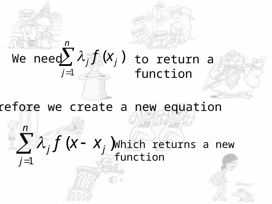
We need

n

jjj xf

1

)(

Therefore we create a new equation

to return a function

Which returns a new function

n

jjj xxf

1

)(

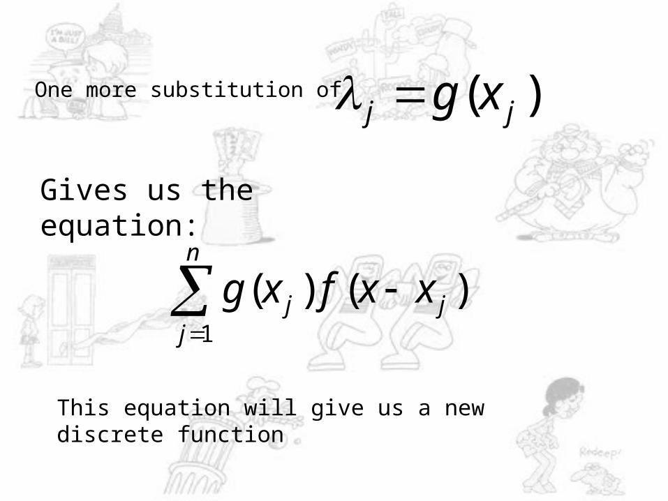
One more substitution of )( jj xg

Gives us the equation:

n

jjj xxfxg

1

)()(

This equation will give us a new discrete function

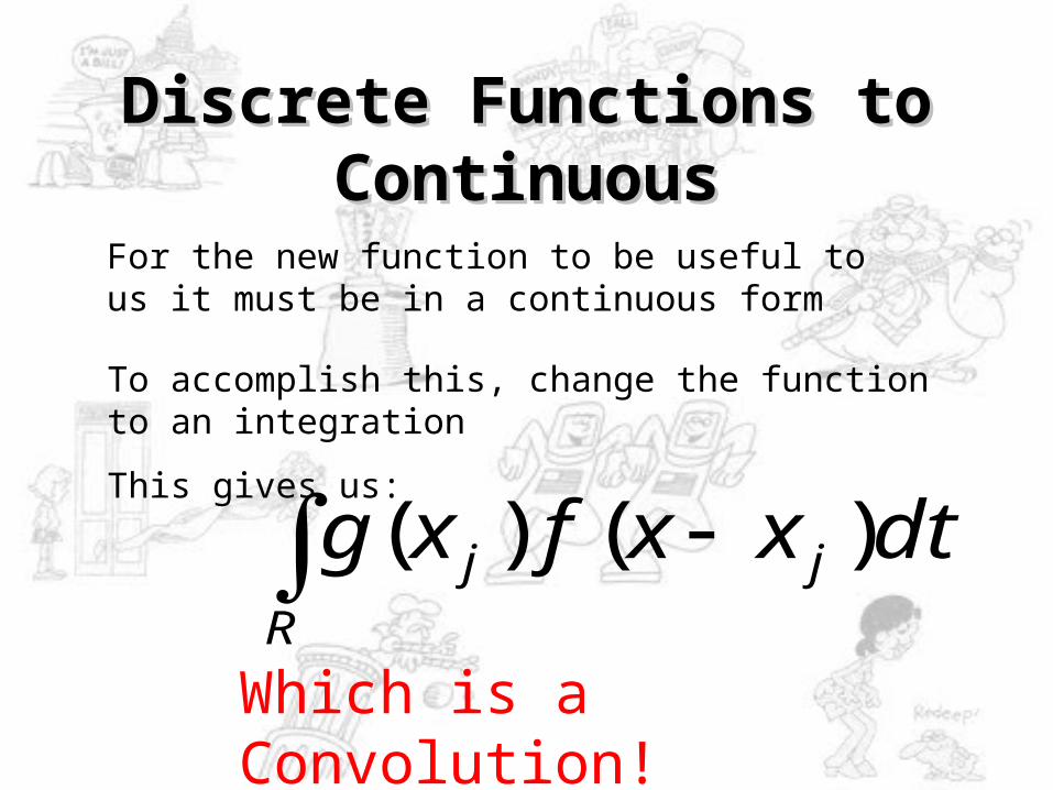
Discrete Functions to Discrete Functions to ContinuousContinuous

For the new function to be useful to us it must be in a continuous form

To accomplish this, change the function to an integration

This gives us:

R

jj dtxxfxg )()(

Which is a Convolution!

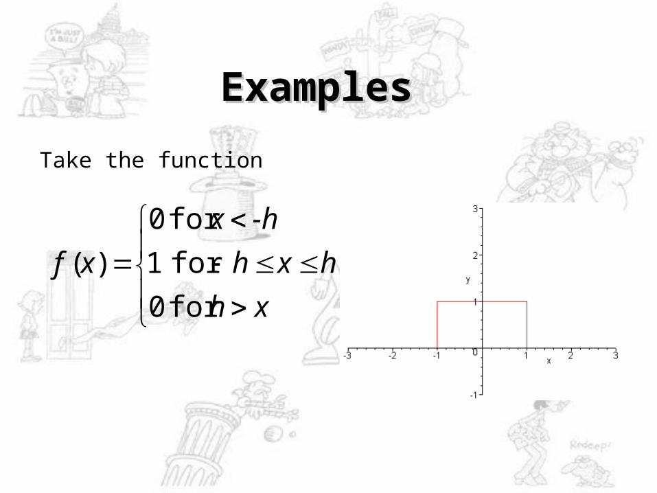
Examples Examples

Take the function

xh

hxh

-hx

xf

for 0

for 1

for 0

)(

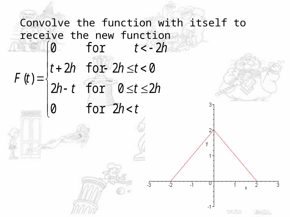
Convolve the function with itself to receive the new function

th

htth

thht

ht

tF

2for 0

20for 2

02for 2

2 for 0

)(

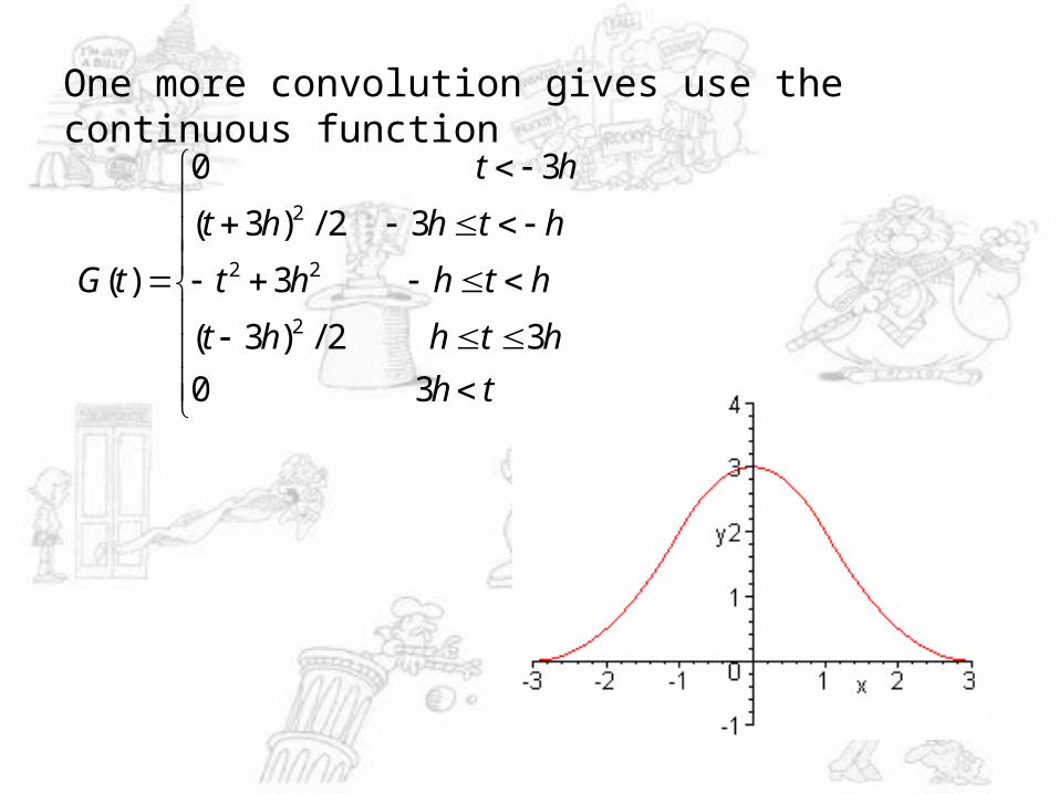
One more convolution gives use the continuous function

th

hthht

hthht

hthht

ht

tG

3 0

3 2/)3(

3

3 2/)3(

3 0

)(2

22

2

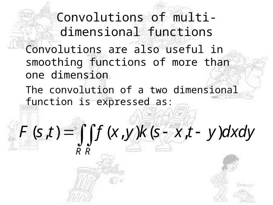
Convolutions of multi-dimensional functions

R R

dxdyytxskyxftsF ),(),(),(

Convolutions are also useful in smoothing functions of more than one dimension

The convolution of a two dimensional function is expressed as:

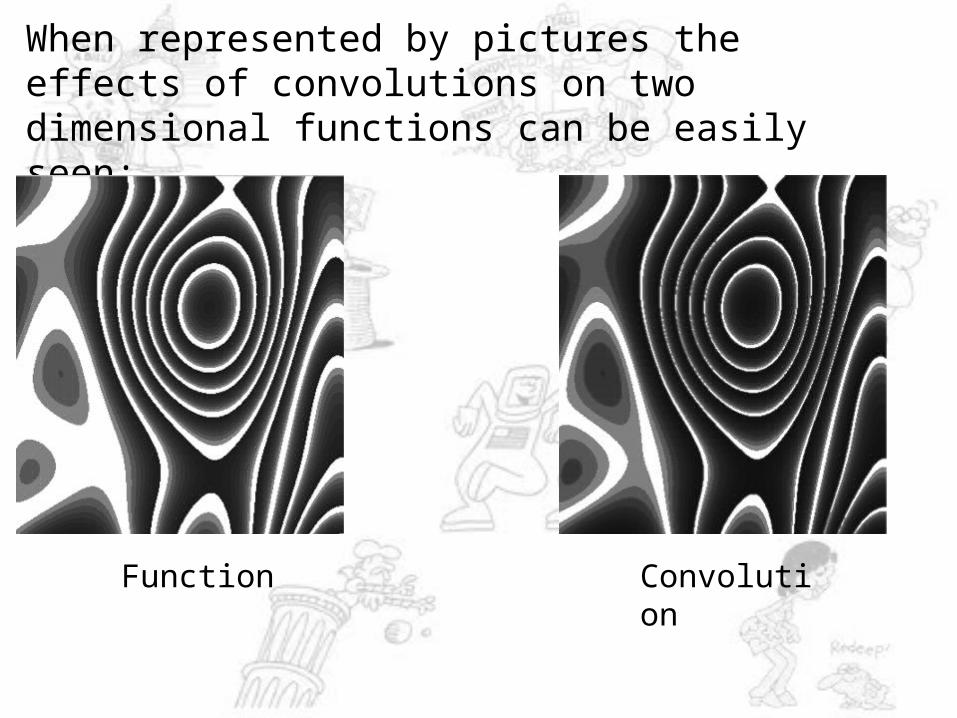
When represented by pictures the effects of convolutions on two dimensional functions can be easily seen:

Function Convolution

Applying Convolutions to Computer Graphics

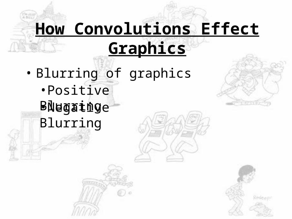
How Convolutions Effect Graphics

• Blurring of graphics•Positive Blurring•Negative Blurring

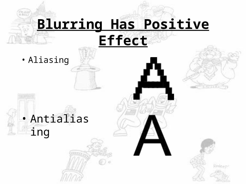
Blurring Has Positive Effect

• Aliasing

• Antialiasing

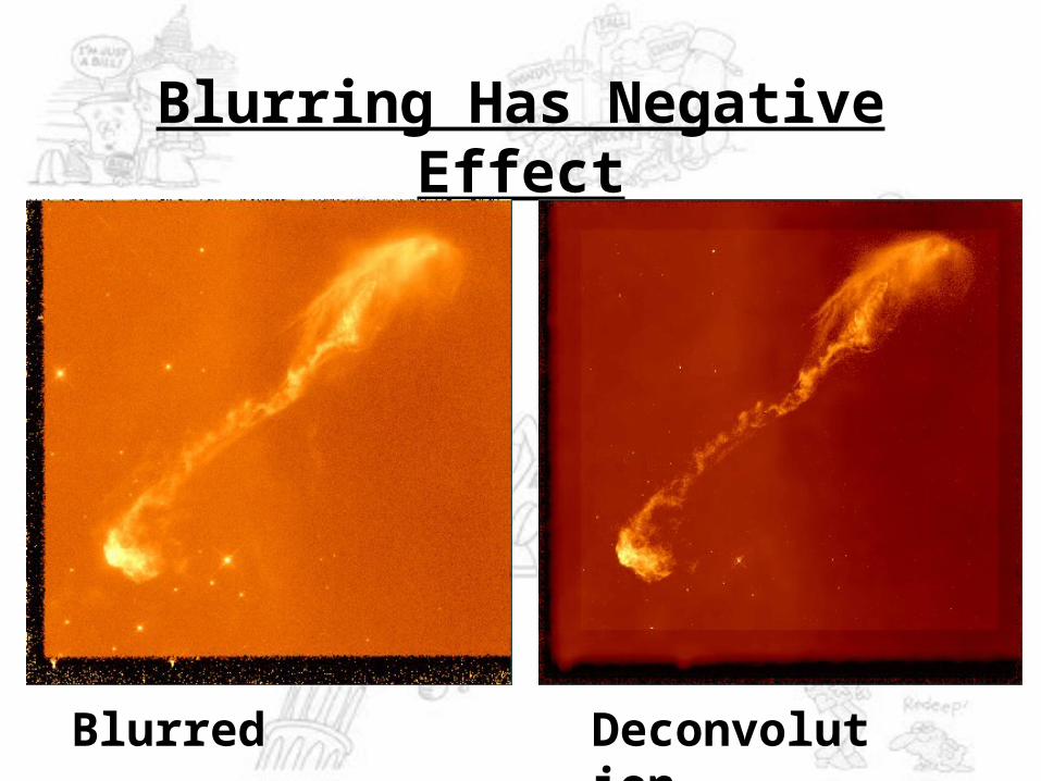
Blurring Has Negative Effect

Blurred Deconvolution

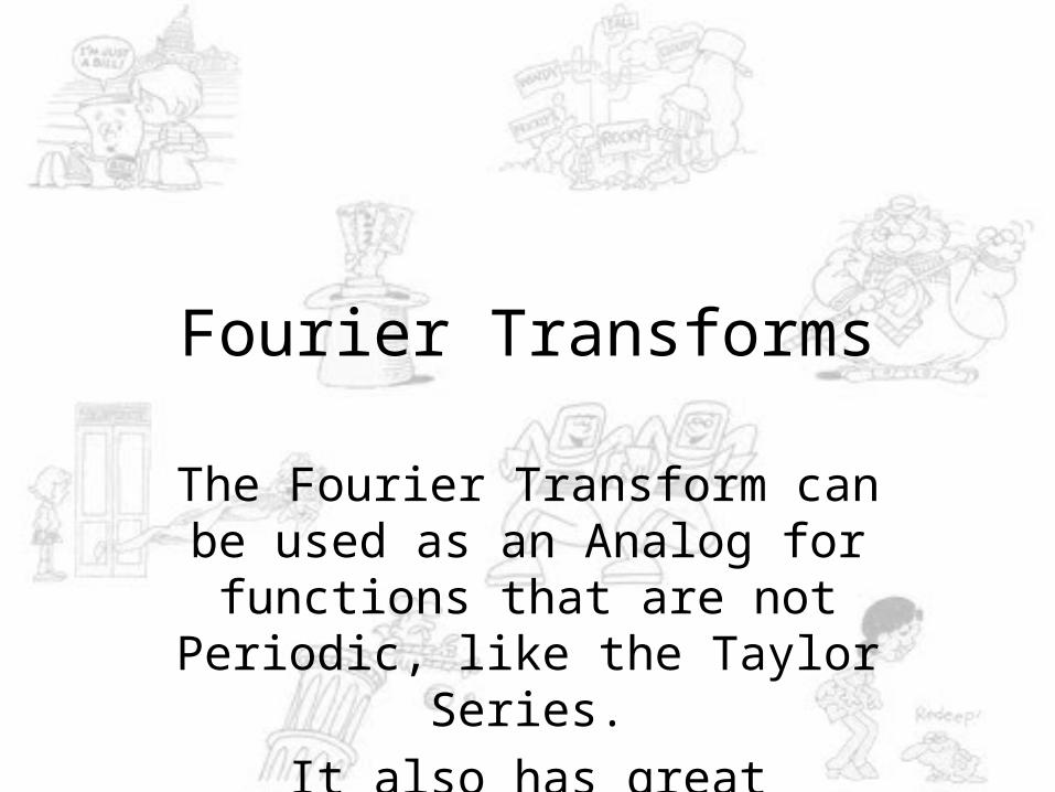
Fourier Transforms

The Fourier Transform can be used as an Analog for functions that are not

Periodic, like the Taylor Series.

It also has great importance in its relation to Convolutions.

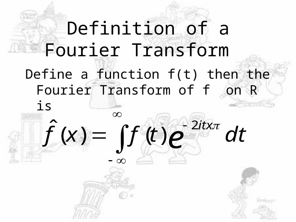
Definition of a Fourier Transform

Define a function f(t) then the Fourier Transform of f on R is

dttfxf eitx2

)()(ˆ

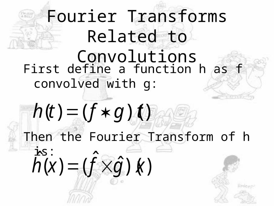
Fourier Transforms Related to Convolutions

First define a function h as f convolved with g:

Then the Fourier Transform of h is:

))(ˆˆ()(ˆ xgfxh

))(()( tgfth

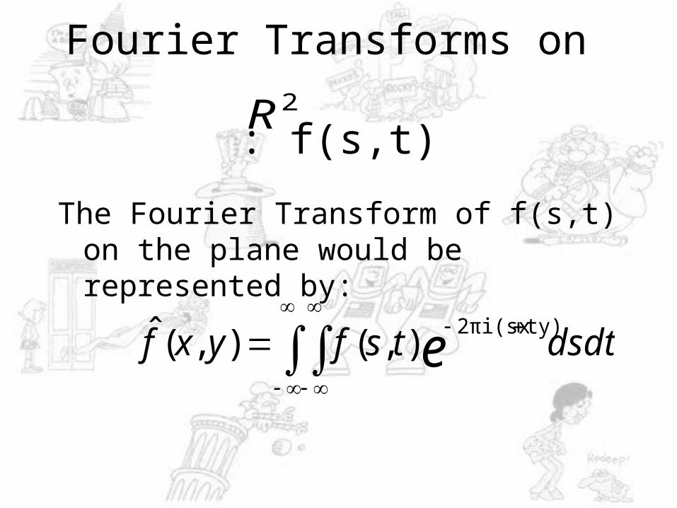
Fourier Transforms on : f(s,t)

The Fourier Transform of f(s,t) on the plane would be represented by:

2R

dsdttsfyxf e

ty)πi(sx2),(),(ˆ

The Diameter of a Star

How can we find it using Convolutions?

Application:

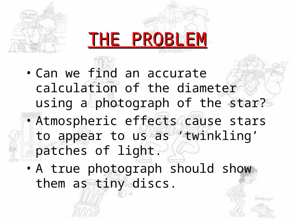
THE PROBLEMTHE PROBLEM

• Can we find an accurate calculation of the diameter using a photograph of the star?

• Atmospheric effects cause stars to appear to us as ‘twinkling’ patches of light.

• A true photograph should show them as tiny discs.

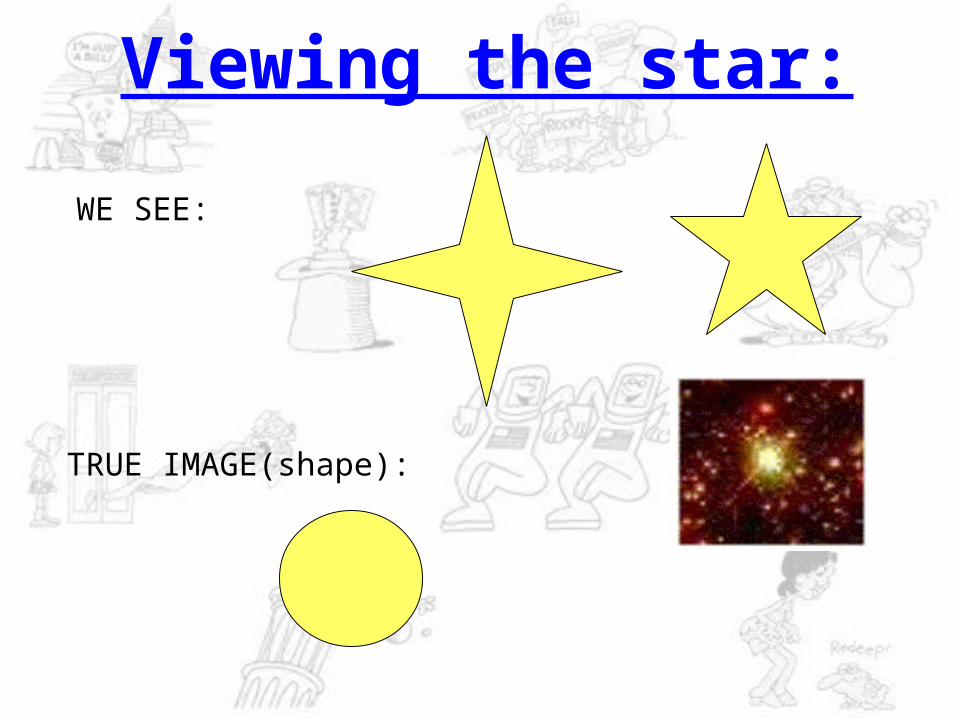
WE SEE:

TRUE IMAGE(shape):

Viewing the star:

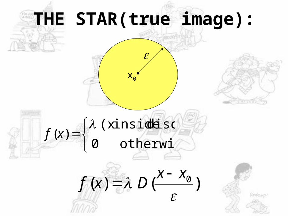
THE STAR(true image):

)()( 0

xx

Dxf

x0

otherwise. 0

disc) inside(x )(

xf

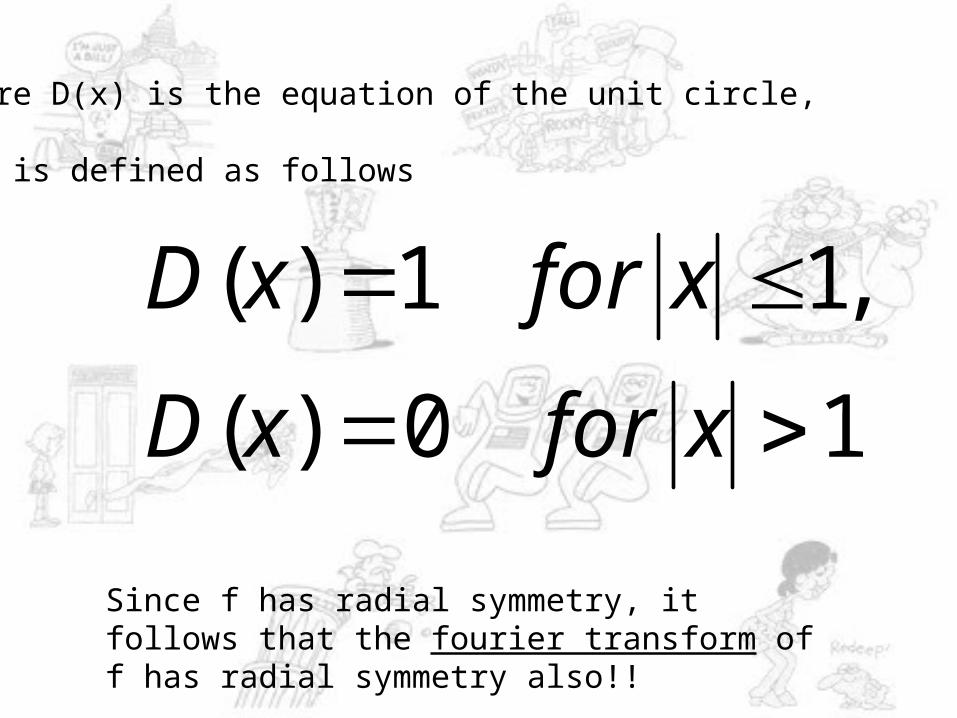
Where D(x) is the equation of the unit circle,

And is defined as follows

10)(

,11)(

xforxD

xforxD

Since f has radial symmetry, it follows that the fourier transform of f has radial symmetry also!!

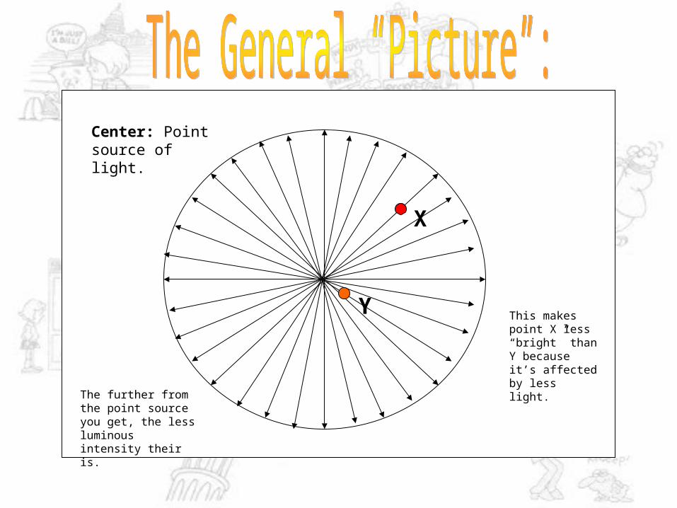
X

The further from the point source you get, the less luminous intensity their is.

This makes point X less “bright” than Y because it’s affected by less light.

Center: Point source of light.

Y

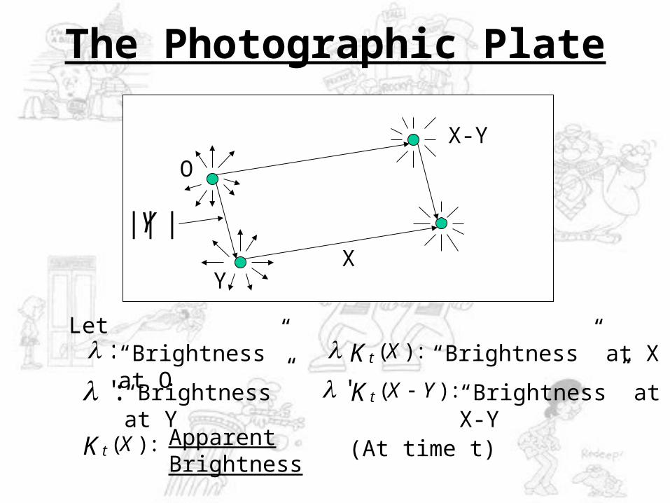
The Photographic Plate

O

XY

X-Y

Let: “Brightness” at O

:' “Brightness” at Y

:)(XK t “Brightness” at X

|||| Y

:)(' YXK t “Brightness” at X-Y

:)(XK tApparent Brightness

True Brightness

(At time t)

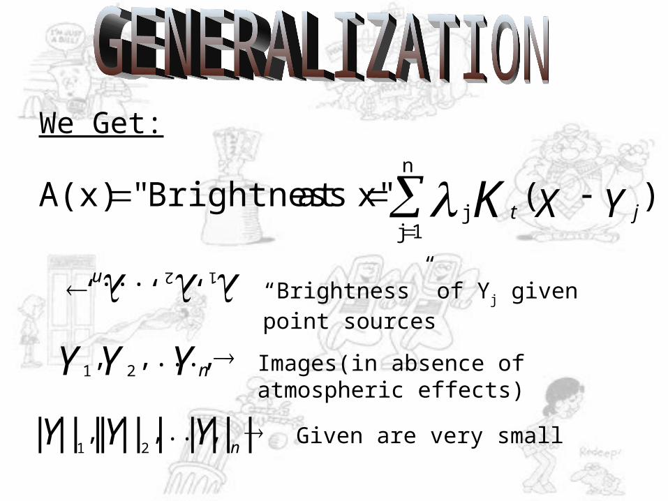
n ,..., ,2 1

YYY n,...,,

21

|||||||||||| ,...,,21

YYY n

“Brightness” of Yj given point sources

Images(in absence of atmospheric effects)

Given are very small

)( at x" Brightness" A(x)n

1jj YX jtK

We Get:

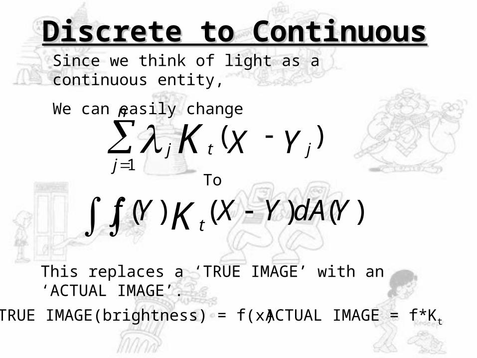
Discrete to ContinuousDiscrete to ContinuousSince we think of light as a continuous entity,

We can easily change

)(1

YX jt

n

jj K

)()()( YdAYXYf K t

To

This replaces a ‘TRUE IMAGE’ with an ‘ACTUAL IMAGE’.

TRUE IMAGE(brightness) = f(x) ACTUAL IMAGE = f*Kt

Continuous form in Detail

)()()( YdAYXYf K t

:)(Yf

:)( YXK t

:)(YdA

Brightness at point Y

Blurring effect(kernel) of the atmosphere at time t.

Integrate with respect to Y

The Convolution:

K tf * =

Where

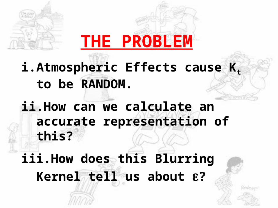
THE PROBLEM

i. Atmospheric Effects cause Kt to be RANDOM.

ii. How can we calculate an accurate representation of this?

iii. How does this Blurring Kernel tell us

about ?

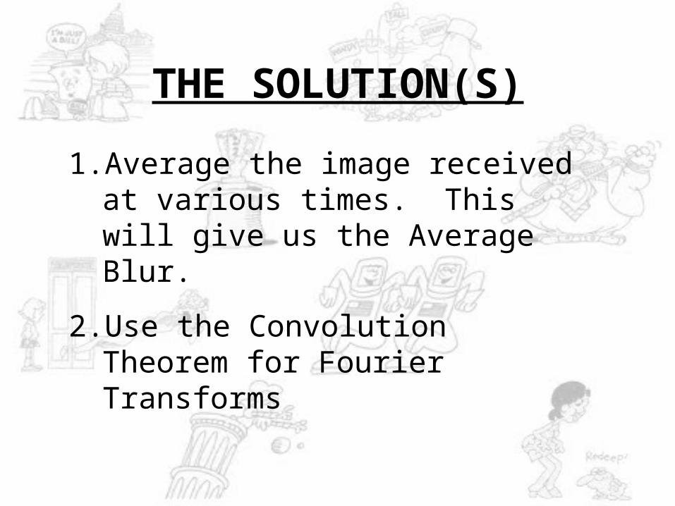
THE SOLUTION(S)

1. Average the image received at various times. This will give us the Average Blur.

2. Use the Convolution Theorem for Fourier Transforms

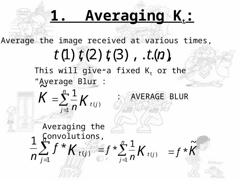
1. Averaging Kt:

Average the image received at various times,

)(),...,3(),2(),1( nttttThis will give a fixed Kt or the “Average Blur”:

KKjt

n

j n )(1

1~

: AVERAGE BLUR

Averaging the Convolutions,

n

jjtKf

n 1)(

*1

K jt

n

j nf

)(1

1*

~

* Kf

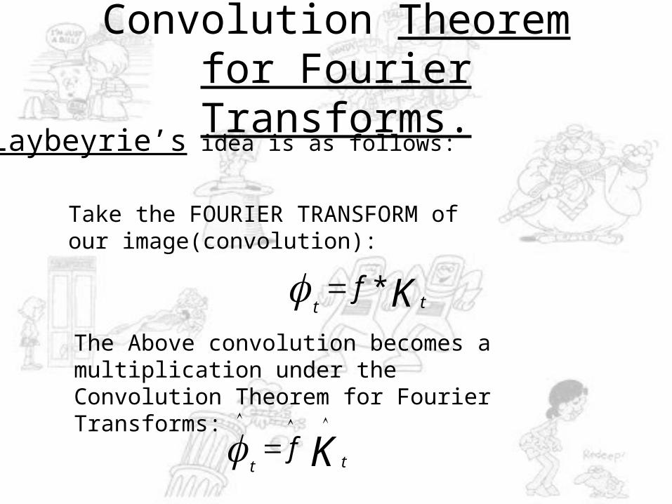
2. Using the Convolution Theorem for Fourier Transforms.

Take the FOURIER TRANSFORM of our image(convolution):

K ttf *

The Above convolution becomes a multiplication under the Convolution Theorem for Fourier Transforms:

K ttf

Laybeyrie’s idea is as follows:

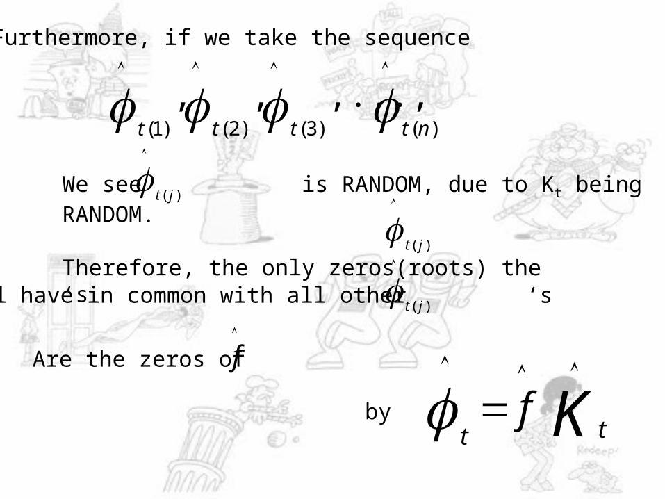
Furthermore, if we take the sequence

)()3()2()1(

,...,,,ntttt

fAre the zeros of

K ttfby

We see is RANDOM, due to Kt being RANDOM.

Therefore, the only zeros(roots) the ‘s

)( jt

)( jt

Will have in common with all other ‘s

)( jt

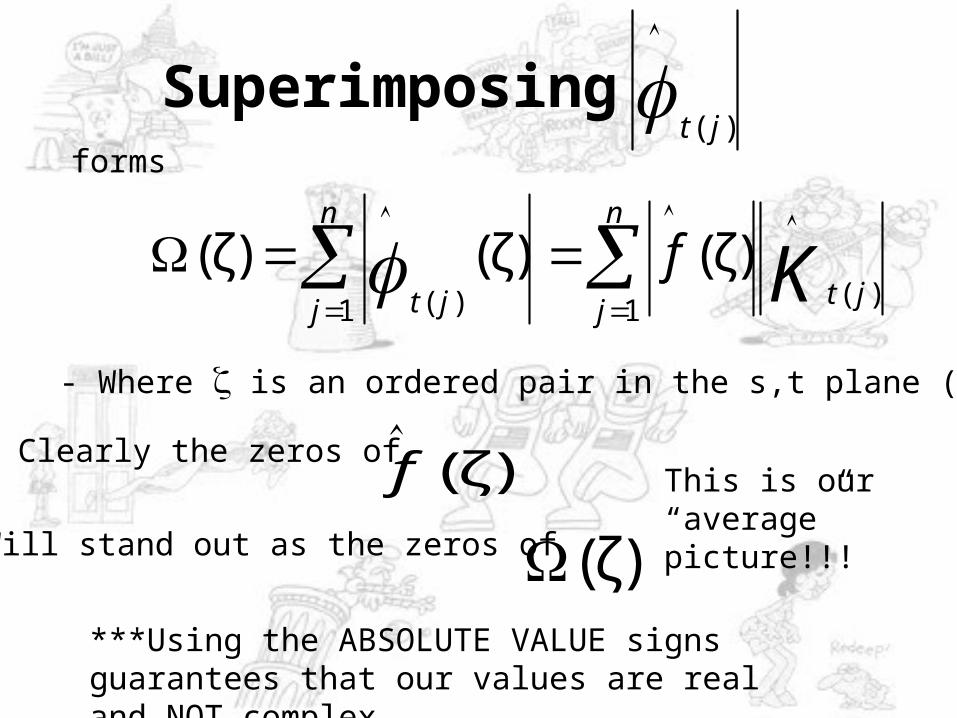
Superimposing

)( jt

forms

K jt

n

j

n

j jtf

)(11 )(

)ζ()ζ()ζ(

Clearly the zeros of )ζ(f

Will stand out as the zeros of )ζ(This is our “average” picture!!!

***Using the ABSOLUTE VALUE signs guarantees that our values are real and NOT complex.

- Where is an ordered pair in the s,t plane (s,t)

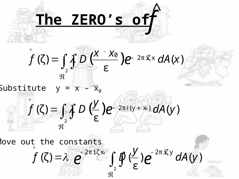
The ZERO’s of f^

)(ε

)ζ(2

xiζπ20)( xdAxx

Df e

Substitute y = x – x0

)(ε

)ζ(2

)xy(π2 0)( ydAy

Df e i

Move out the constants

)()ε

()ζ(2

yiζπ2xζiπ2 0

ydAy

Df ee

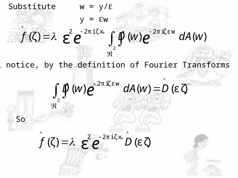
)()()ζ(2

wεiζπ2xζiπ22 0

ε wdAwDf ee

Substitute w = y/ y = w

You’ll notice, by the definition of Fourier Transforms

)εζ()()(2

wεiζπ2

DwdAwD e

So

)εζ()ζ(0xζiπ22

ε

Df e

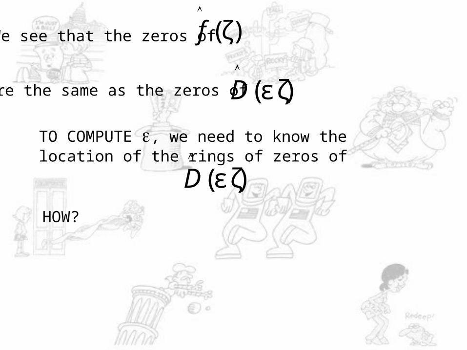
We see that the zeros of )ζ(f

Are the same as the zeros of )εζ(D

TO COMPUTE , we need to know the location of the rings of zeros of

)εζ(D

HOW?

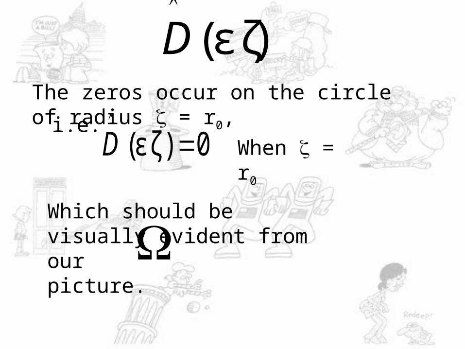
)εζ(D

The zeros occur on the circle of radius = r0,

Which should be visually evident from our picture.

i.e. 0)εζ(

D When = r0

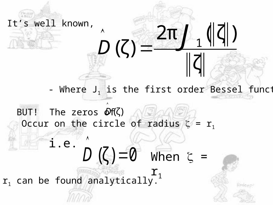
It’s well known,

ζ

)ζ(π2)ζ( 1JD

- Where J1 is the first order Bessel function

BUT! The zeros of )ζ(D

Occur on the circle of radius = r1

i.e. 0)ζ(

D When = r1

r1 can be found analytically.

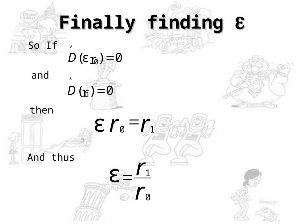
Finally finding Finally finding So If

0)rε( 0 D

and

0)r( 1

D

then

rr 10ε

rr

0

1ε And thus

Thank you for your cooperation.

References

• “Fourier Analysis” by T.W. Korner, Cambridge University Press, 1988

• “Convolutions and Computer Graphics” by Anne M. Burns,

• Dr. Steve Deckelman