“What’s New in Econometrics”

Lecture 5

Instrumental Variables with Treatment Effect

Heterogeneity: Local Average Treatment Effects

Guido Imbens

NBER Summer Institute, 2007

Outline

1. Introduction

2. Basics

3. Local Average Treatment Effects

4. Extrapolation to the Population

5. Covariates

6. Multivalued Instruments

7. Multivalued Endogenous Regressors

1

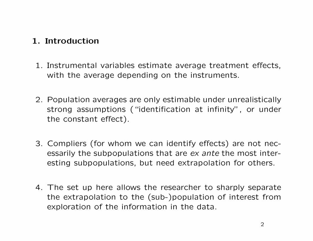
1. Introduction

1. Instrumental variables estimate average treatment effects,with the average depending on the instruments.

2. Population averages are only estimable under unrealisticallystrong assumptions (“identification at infinity”, or underthe constant effect).

3. Compliers (for whom we can identify effects) are not nec-essarily the subpopulations that are ex ante the most inter-esting subpopulations, but need extrapolation for others.

4. The set up here allows the researcher to sharply separatethe extrapolation to the (sub-)population of interest fromexploration of the information in the data.

2

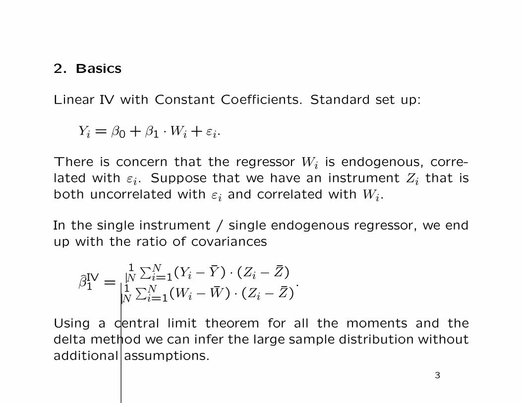
2. Basics

Linear IV with Constant Coefficients. Standard set up:

Yi = β0 + β1 · Wi + εi.

There is concern that the regressor Wi is endogenous, corre-lated with εi. Suppose that we have an instrument Zi that isboth uncorrelated with εi and correlated with Wi.

In the single instrument / single endogenous regressor, we endup with the ratio of covariances

βIV1 =

1N

∑Ni=1(Yi − Y ) · (Zi − Z)

1N

∑Ni=1(Wi − W ) · (Zi − Z)

.

Using a central limit theorem for all the moments and thedelta method we can infer the large sample distribution withoutadditional assumptions.

3

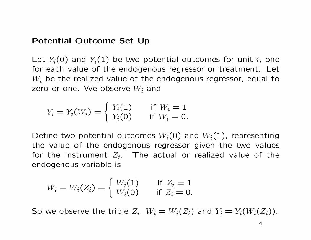
Potential Outcome Set Up

Let Yi(0) and Yi(1) be two potential outcomes for unit i, onefor each value of the endogenous regressor or treatment. LetWi be the realized value of the endogenous regressor, equal tozero or one. We observe Wi and

Yi = Yi(Wi) =

{Yi(1) if Wi = 1Yi(0) if Wi = 0.

Define two potential outcomes Wi(0) and Wi(1), representingthe value of the endogenous regressor given the two valuesfor the instrument Zi. The actual or realized value of theendogenous variable is

Wi = Wi(Zi) =

{Wi(1) if Zi = 1Wi(0) if Zi = 0.

So we observe the triple Zi, Wi = Wi(Zi) and Yi = Yi(Wi(Zi)).

4

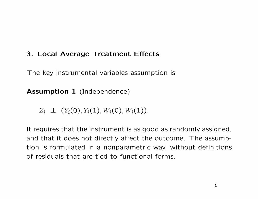
3. Local Average Treatment Effects

The key instrumental variables assumption is

Assumption 1 (Independence)

Zi ⊥⊥ (Yi(0), Yi(1), Wi(0), Wi(1)).

It requires that the instrument is as good as randomly assigned,

and that it does not directly affect the outcome. The assump-

tion is formulated in a nonparametric way, without definitions

of residuals that are tied to functional forms.

5

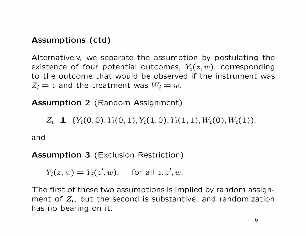
Assumptions (ctd)

Alternatively, we separate the assumption by postulating theexistence of four potential outcomes, Yi(z, w), correspondingto the outcome that would be observed if the instrument wasZi = z and the treatment was Wi = w.

Assumption 2 (Random Assignment)

Zi ⊥⊥ (Yi(0,0), Yi(0,1), Yi(1,0), Yi(1,1), Wi(0), Wi(1)).

and

Assumption 3 (Exclusion Restriction)

Yi(z, w) = Yi(z′, w), for all z, z′, w.

The first of these two assumptions is implied by random assign-ment of Zi, but the second is substantive, and randomizationhas no bearing on it.

6

Compliance Types

It is useful for our approach to think about the compliance

behavior of the different units

Wi(0)0 1

0 never-taker defierWi(1)

1 complier always-taker

7

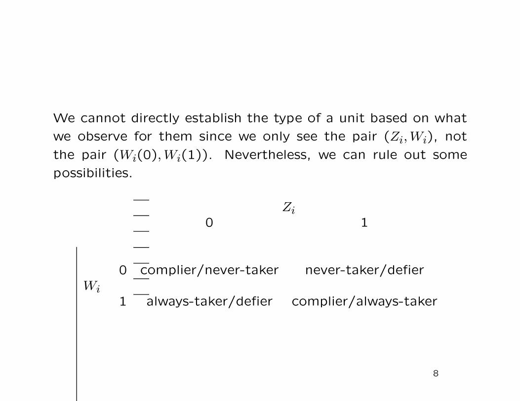
We cannot directly establish the type of a unit based on what

we observe for them since we only see the pair (Zi, Wi), not

the pair (Wi(0), Wi(1)). Nevertheless, we can rule out some

possibilities.

Zi0 1

0 complier/never-taker never-taker/defierWi

1 always-taker/defier complier/always-taker

8

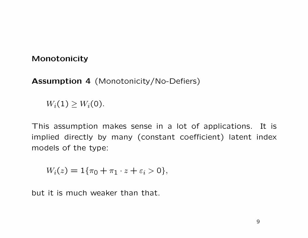
Monotonicity

Assumption 4 (Monotonicity/No-Defiers)

Wi(1) ≥ Wi(0).

This assumption makes sense in a lot of applications. It is

implied directly by many (constant coefficient) latent index

models of the type:

Wi(z) = 1{π0 + π1 · z + εi > 0},

but it is much weaker than that.

9

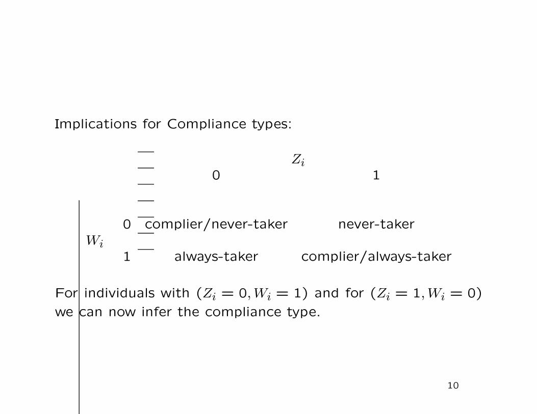
Implications for Compliance types:

Zi0 1

0 complier/never-taker never-takerWi

1 always-taker complier/always-taker

For individuals with (Zi = 0, Wi = 1) and for (Zi = 1, Wi = 0)

we can now infer the compliance type.

10

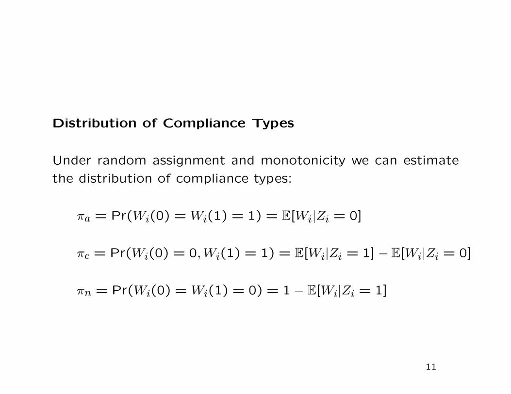
Distribution of Compliance Types

Under random assignment and monotonicity we can estimate

the distribution of compliance types:

πa = Pr(Wi(0) = Wi(1) = 1) = E[Wi|Zi = 0]

πc = Pr(Wi(0) = 0, Wi(1) = 1) = E[Wi|Zi = 1] − E[Wi|Zi = 0]

πn = Pr(Wi(0) = Wi(1) = 0) = 1 − E[Wi|Zi = 1]

11

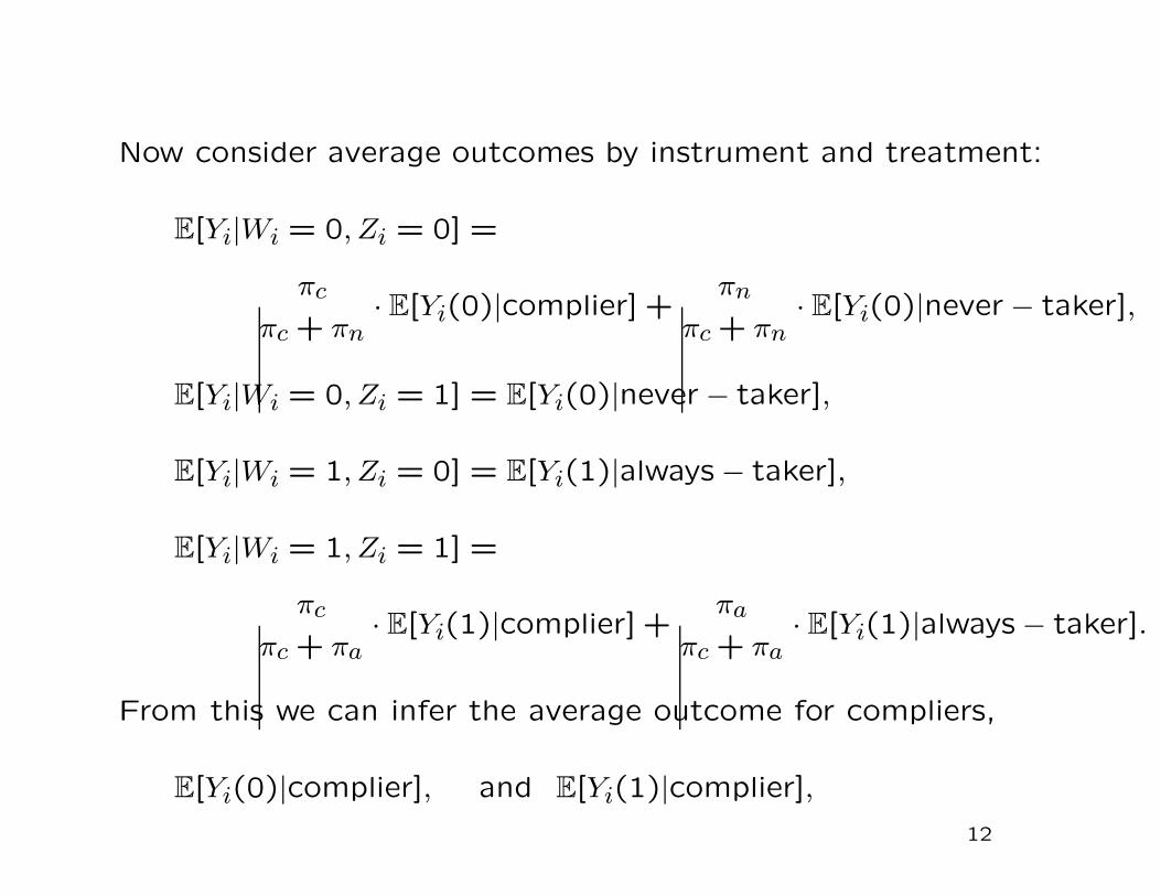
Now consider average outcomes by instrument and treatment:

E[Yi|Wi = 0, Zi = 0] =

πc

πc + πn· E[Yi(0)|complier] +

πn

πc + πn· E[Yi(0)|never − taker],

E[Yi|Wi = 0, Zi = 1] = E[Yi(0)|never − taker],

E[Yi|Wi = 1, Zi = 0] = E[Yi(1)|always − taker],

E[Yi|Wi = 1, Zi = 1] =

πc

πc + πa· E[Yi(1)|complier] +

πa

πc + πa· E[Yi(1)|always − taker].

From this we can infer the average outcome for compliers,

E[Yi(0)|complier], and E[Yi(1)|complier],

12

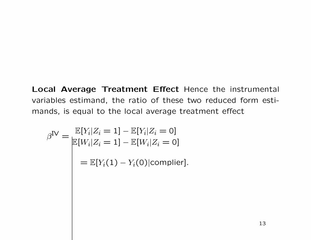
Local Average Treatment Effect Hence the instrumental

variables estimand, the ratio of these two reduced form esti-

mands, is equal to the local average treatment effect

βIV =E[Yi|Zi = 1]− E[Yi|Zi = 0]

E[Wi|Zi = 1]− E[Wi|Zi = 0]

= E[Yi(1)− Yi(0)|complier].

13

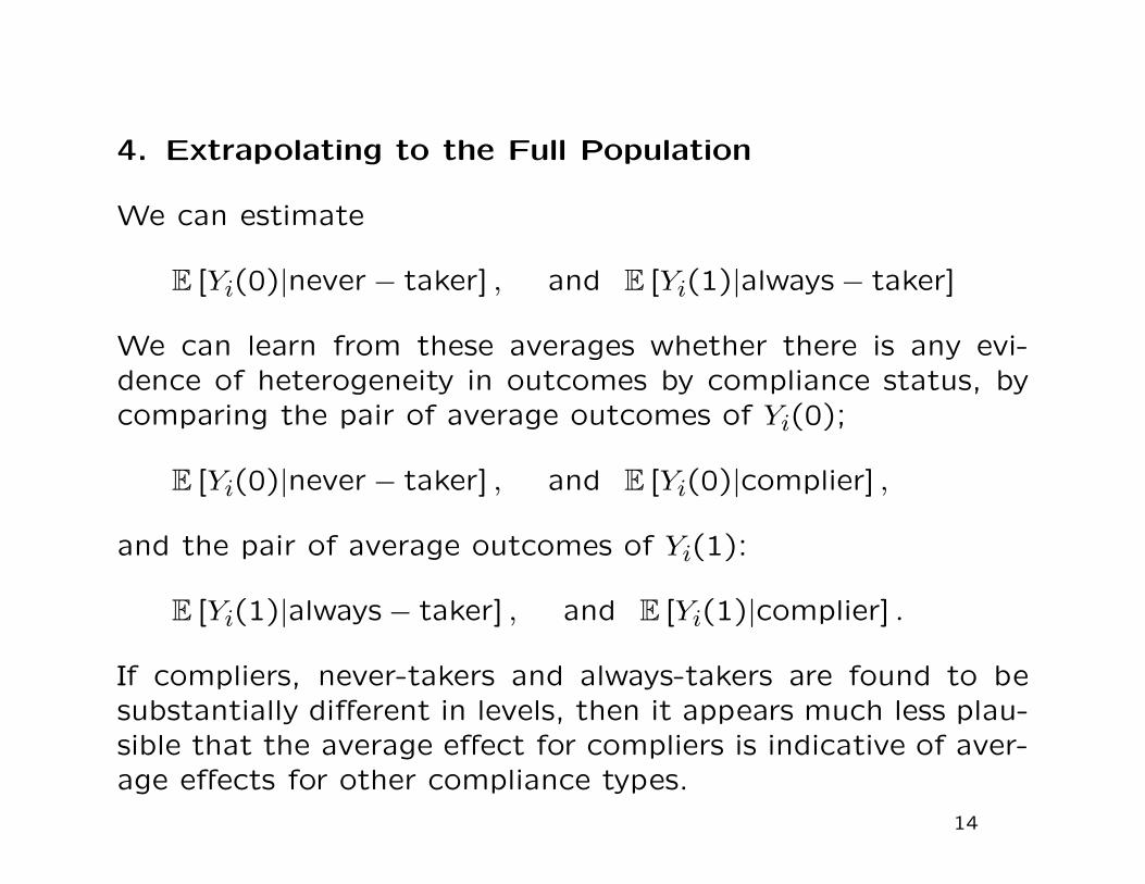
4. Extrapolating to the Full Population

We can estimate

E [Yi(0)|never − taker] , and E [Yi(1)|always − taker]

We can learn from these averages whether there is any evi-dence of heterogeneity in outcomes by compliance status, bycomparing the pair of average outcomes of Yi(0);

E [Yi(0)|never − taker] , and E [Yi(0)|complier] ,

and the pair of average outcomes of Yi(1):

E [Yi(1)|always − taker] , and E [Yi(1)|complier] .

If compliers, never-takers and always-takers are found to besubstantially different in levels, then it appears much less plau-sible that the average effect for compliers is indicative of aver-age effects for other compliance types.

14

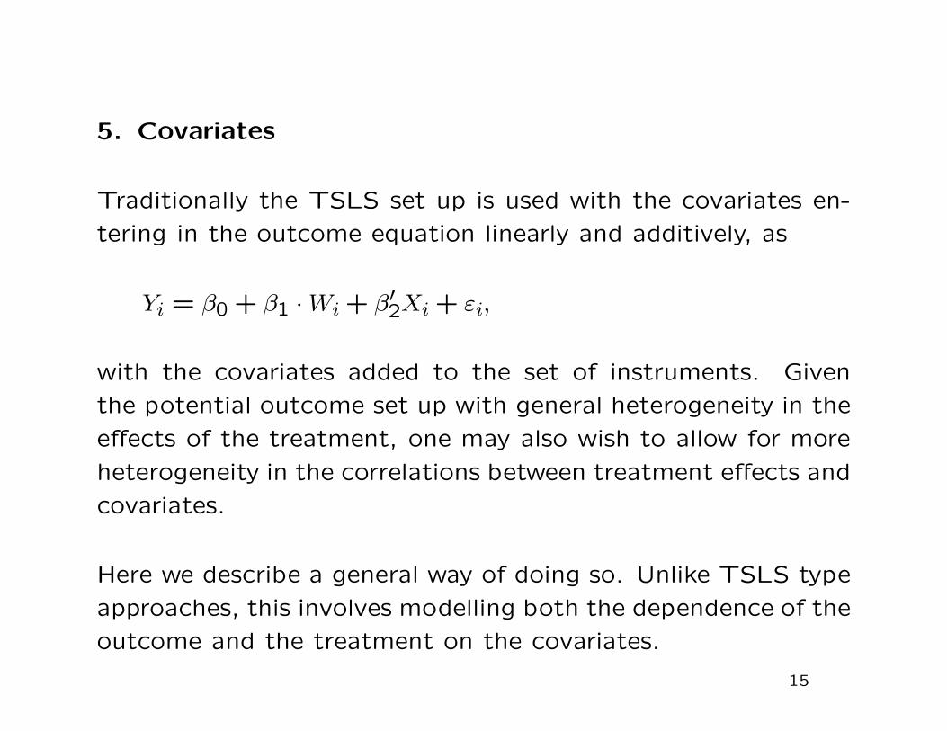
5. Covariates

Traditionally the TSLS set up is used with the covariates en-

tering in the outcome equation linearly and additively, as

Yi = β0 + β1 · Wi + β′2Xi + εi,

with the covariates added to the set of instruments. Given

the potential outcome set up with general heterogeneity in the

effects of the treatment, one may also wish to allow for more

heterogeneity in the correlations between treatment effects and

covariates.

Here we describe a general way of doing so. Unlike TSLS type

approaches, this involves modelling both the dependence of the

outcome and the treatment on the covariates.

15

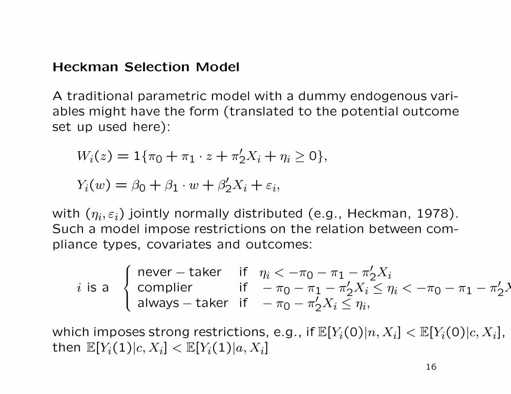
Heckman Selection Model

A traditional parametric model with a dummy endogenous vari-ables might have the form (translated to the potential outcomeset up used here):

Wi(z) = 1{π0 + π1 · z + π′2Xi + ηi ≥ 0},

Yi(w) = β0 + β1 · w + β′2Xi + εi,

with (ηi, εi) jointly normally distributed (e.g., Heckman, 1978).Such a model impose restrictions on the relation between com-pliance types, covariates and outcomes:

i is a

⎧⎪⎨⎪⎩never − taker if ηi < −π0 − π1 − π′

2Xicomplier if − π0 − π1 − π′

2Xi ≤ ηi < −π0 − π1 − π′2X

always− taker if − π0 − π′2Xi ≤ ηi,

which imposes strong restrictions, e.g., if E[Yi(0)|n, Xi] < E[Yi(0)|c, Xi],then E[Yi(1)|c, Xi] < E[Yi(1)|a, Xi]

16

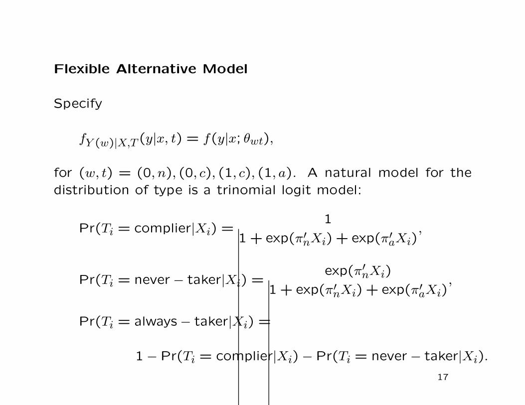
Flexible Alternative Model

Specify

fY (w)|X,T (y|x, t) = f(y|x; θwt),

for (w, t) = (0, n), (0, c), (1, c), (1, a). A natural model for thedistribution of type is a trinomial logit model:

Pr(Ti = complier|Xi) =1

1 + exp(π′nXi) + exp(π′

aXi),

Pr(Ti = never − taker|Xi) =exp(π′

nXi)

1 + exp(π′nXi) + exp(π′

aXi),

Pr(Ti = always − taker|Xi) =

1 − Pr(Ti = complier|Xi) − Pr(Ti = never − taker|Xi).

17

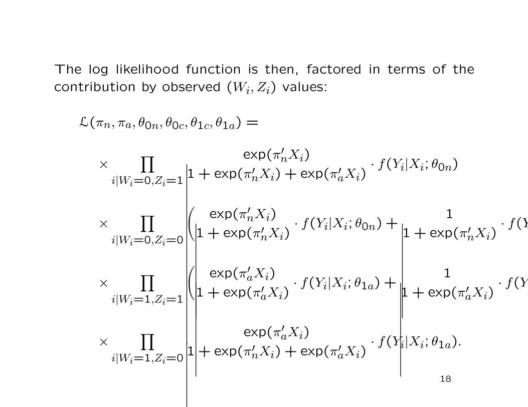
The log likelihood function is then, factored in terms of thecontribution by observed (Wi, Zi) values:

L(πn, πa, θ0n, θ0c, θ1c, θ1a) =

× ∏i|Wi=0,Zi=1

exp(π′nXi)

1 + exp(π′nXi) + exp(π′

aXi)· f(Yi|Xi; θ0n)

× ∏i|Wi=0,Zi=0

(exp(π′

nXi)

1 + exp(π′nXi)

· f(Yi|Xi; θ0n) +1

1 + exp(π′nXi)

· f(Y

× ∏i|Wi=1,Zi=1

(exp(π′

aXi)

1 + exp(π′aXi)

· f(Yi|Xi; θ1a) +1

1 + exp(π′aXi)

· f(Y

× ∏i|Wi=1,Zi=0

exp(π′aXi)

1 + exp(π′nXi) + exp(π′

aXi)· f(Yi|Xi; θ1a).

18

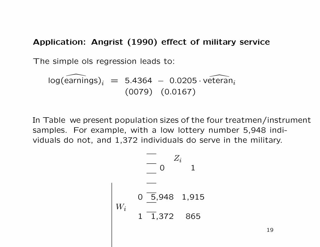
Application: Angrist (1990) effect of military service

The simple ols regression leads to:

log(earnings)i = 5.4364 − 0.0205 · veterani

(0079) (0.0167)

In Table we present population sizes of the four treatmen/instrumentsamples. For example, with a low lottery number 5,948 indi-viduals do not, and 1,372 individuals do serve in the military.

Zi0 1

0 5,948 1,915Wi

1 1,372 865

19

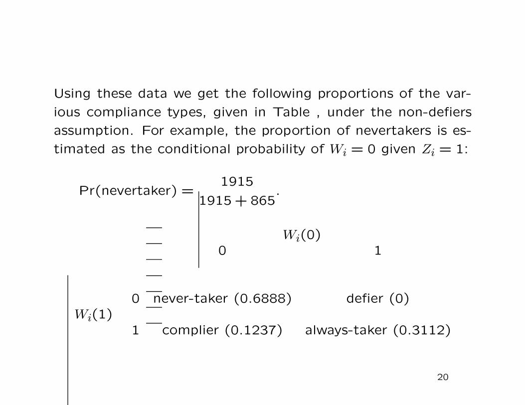
Using these data we get the following proportions of the var-

ious compliance types, given in Table , under the non-defiers

assumption. For example, the proportion of nevertakers is es-

timated as the conditional probability of Wi = 0 given Zi = 1:

Pr(nevertaker) =1915

1915 + 865.

Wi(0)0 1

0 never-taker (0.6888) defier (0)Wi(1)

1 complier (0.1237) always-taker (0.3112)

20

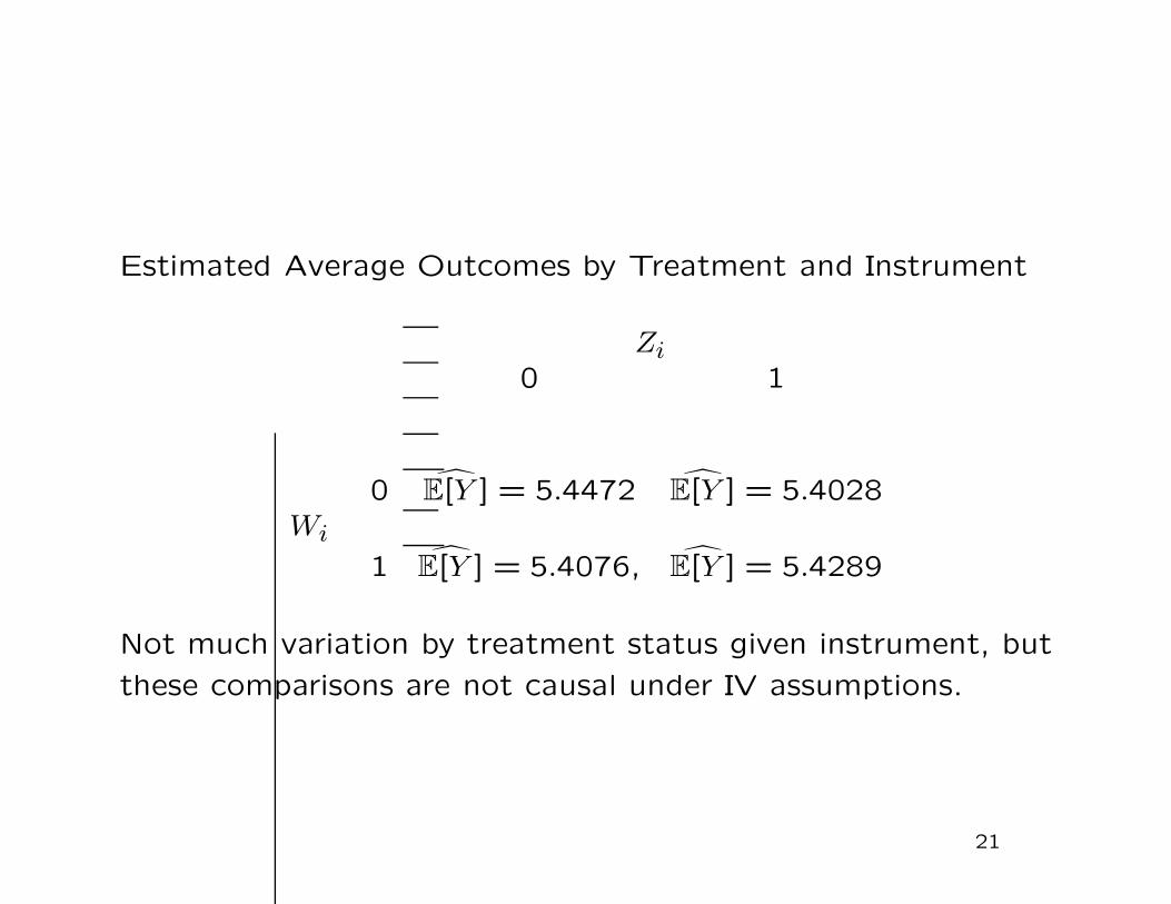
Estimated Average Outcomes by Treatment and Instrument

Zi0 1

0 E[Y ] = 5.4472 E[Y ] = 5.4028Wi

1 E[Y ] = 5.4076, E[Y ] = 5.4289

Not much variation by treatment status given instrument, but

these comparisons are not causal under IV assumptions.

21

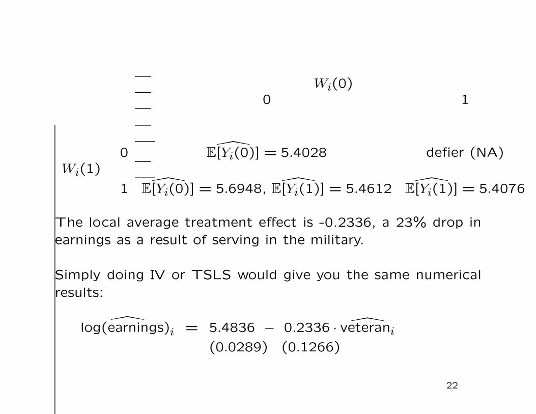
Wi(0)0 1

0 E[Yi(0)] = 5.4028 defier (NA)Wi(1)

1 E[Yi(0)] = 5.6948, E[Yi(1)] = 5.4612 E[Yi(1)] = 5.4076

The local average treatment effect is -0.2336, a 23% drop inearnings as a result of serving in the military.

Simply doing IV or TSLS would give you the same numericalresults:

log(earnings)i = 5.4836 − 0.2336 · veterani

(0.0289) (0.1266)

22

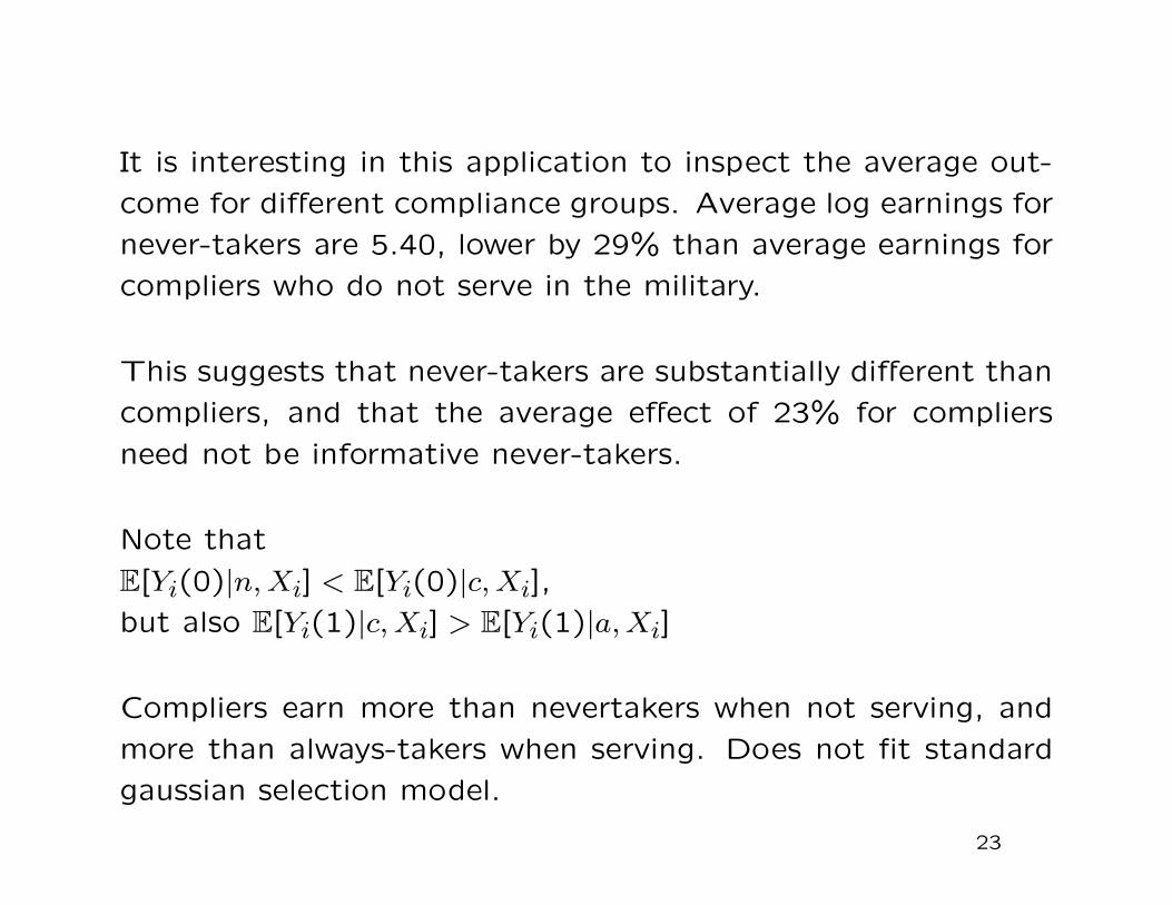
It is interesting in this application to inspect the average out-

come for different compliance groups. Average log earnings for

never-takers are 5.40, lower by 29% than average earnings for

compliers who do not serve in the military.

This suggests that never-takers are substantially different than

compliers, and that the average effect of 23% for compliers

need not be informative never-takers.

Note that

E[Yi(0)|n, Xi] < E[Yi(0)|c, Xi],

but also E[Yi(1)|c, Xi] > E[Yi(1)|a, Xi]

Compliers earn more than nevertakers when not serving, and

more than always-takers when serving. Does not fit standard

gaussian selection model.

23

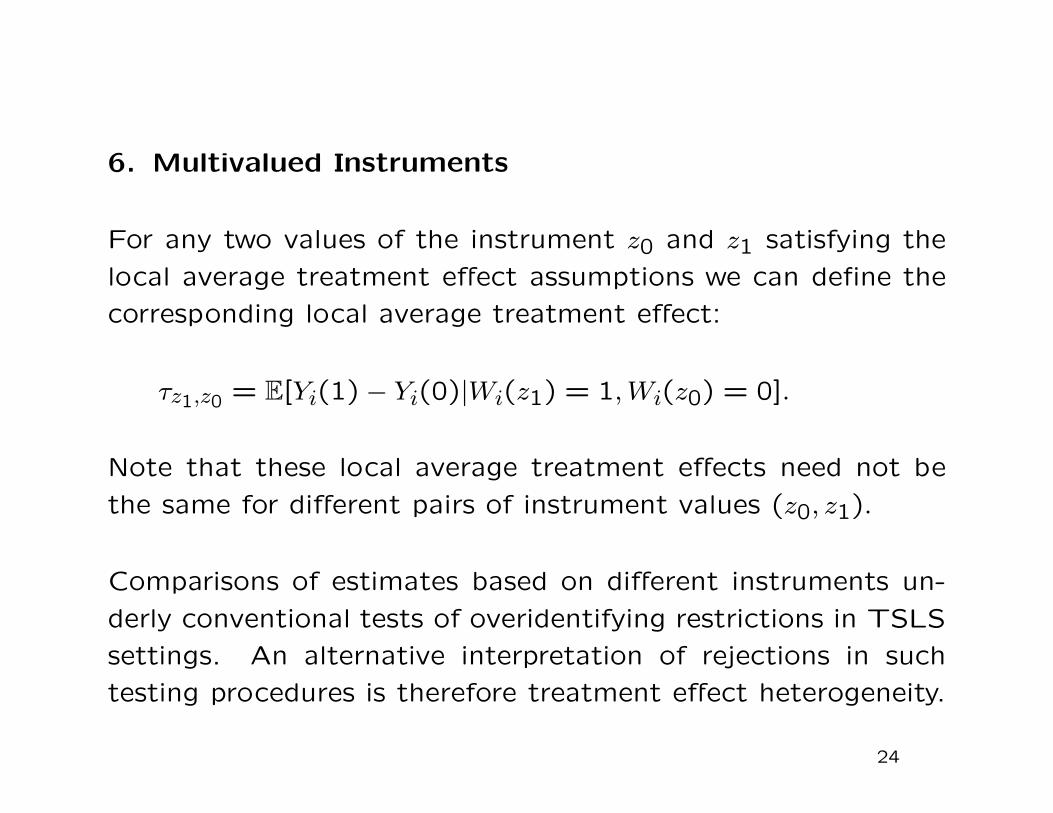
6. Multivalued Instruments

For any two values of the instrument z0 and z1 satisfying the

local average treatment effect assumptions we can define the

corresponding local average treatment effect:

τz1,z0 = E[Yi(1) − Yi(0)|Wi(z1) = 1, Wi(z0) = 0].

Note that these local average treatment effects need not be

the same for different pairs of instrument values (z0, z1).

Comparisons of estimates based on different instruments un-

derly conventional tests of overidentifying restrictions in TSLS

settings. An alternative interpretation of rejections in such

testing procedures is therefore treatment effect heterogeneity.

24

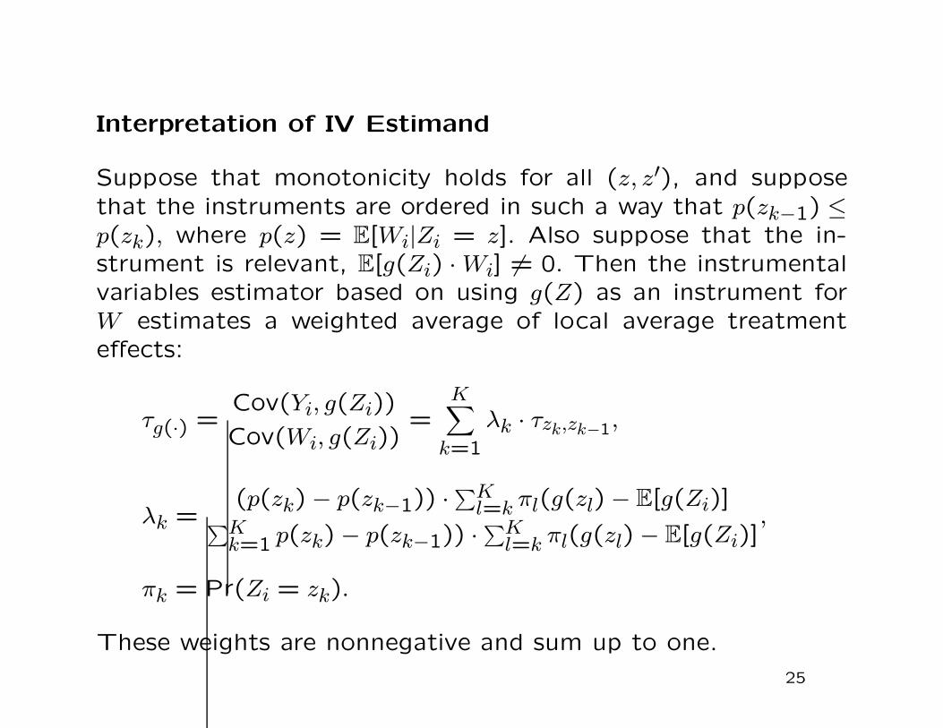
Interpretation of IV Estimand

Suppose that monotonicity holds for all (z, z′), and supposethat the instruments are ordered in such a way that p(zk−1) ≤p(zk), where p(z) = E[Wi|Zi = z]. Also suppose that the in-strument is relevant, E[g(Zi) · Wi] �= 0. Then the instrumentalvariables estimator based on using g(Z) as an instrument forW estimates a weighted average of local average treatmenteffects:

τg(·) =Cov(Yi, g(Zi))

Cov(Wi, g(Zi))=

K∑k=1

λk · τzk,zk−1,

λk =(p(zk) − p(zk−1)) ·

∑Kl=k πl(g(zl) − E[g(Zi)]∑K

k=1 p(zk) − p(zk−1)) ·∑K

l=k πl(g(zl) − E[g(Zi)],

πk = Pr(Zi = zk).

These weights are nonnegative and sum up to one.

25

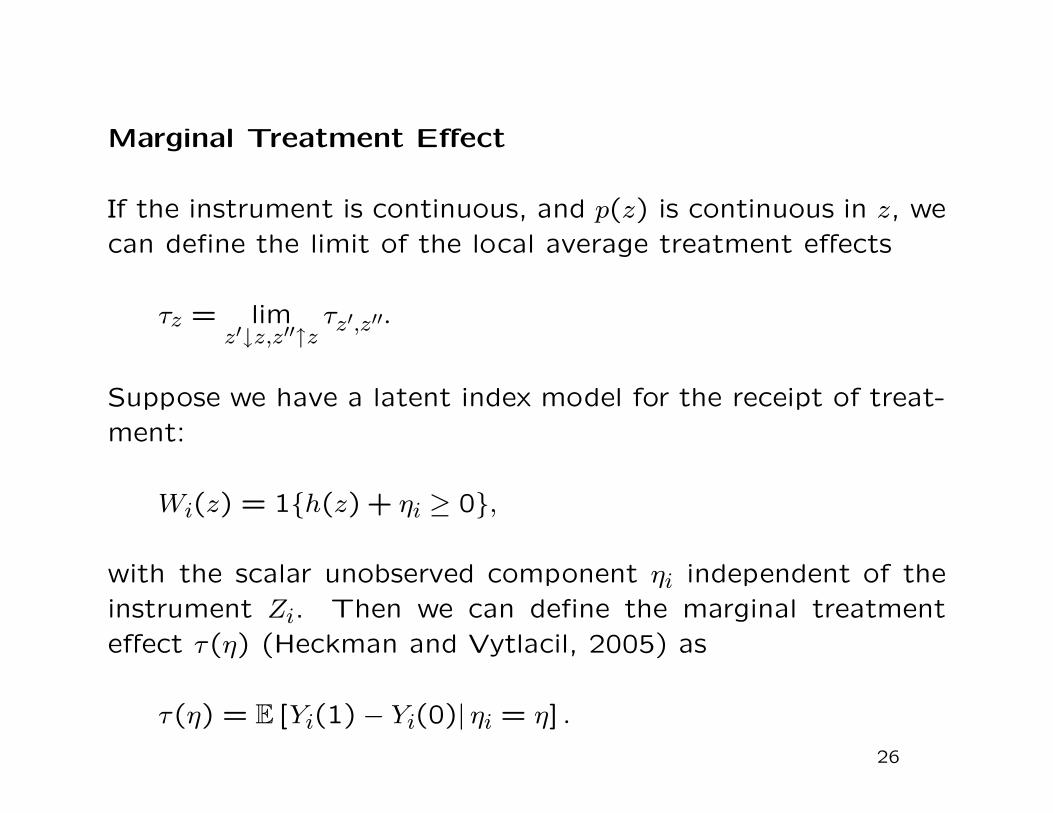
Marginal Treatment Effect

If the instrument is continuous, and p(z) is continuous in z, wecan define the limit of the local average treatment effects

τz = limz′↓z,z′′↑z

τz′,z′′.

Suppose we have a latent index model for the receipt of treat-ment:

Wi(z) = 1{h(z) + ηi ≥ 0},

with the scalar unobserved component ηi independent of theinstrument Zi. Then we can define the marginal treatmenteffect τ(η) (Heckman and Vytlacil, 2005) as

τ(η) = E [Yi(1) − Yi(0)| ηi = η] .

26

This marginal treatment effect relates directly to the limit of

the local average treatment effects

τ(η) = τz, with η = −h(z)).

Note that we can only define this for values of η for which there

is a z such that τ = −h(z).

Normalizing the marginal distribution of η to be uniform on

[0,1], this restricts η to be in the interval [infz p(z), supz p(z)],

where p(z) = Pr(Wi = 1|Zi = z).

Now we can characterize various average treatment effects in

terms of this limit. E.g.:

τ =∫η

τ(η)dFη(η).

27

7. Multivalued Endogenous Variables

τ =Cov(Yi, Zi)

Cov(Wi, Zi)=

E[Yi|Zi = 1]− E[Yi|Zi = 0]

E[Wi|Zi = 1]− E[Wi|Zi = 0].

Exclusion restriction and monotonicity:

Yi(w) Wi(z) ⊥⊥ Zi, Wi(1) ≥ Wi(0),

Then

τ =J∑

j=1

λj · E[Yi(j)− Yi(j − 1)|Wi(1) ≥ j > Wi(0)],

λj =Pr(Wi(1) ≥ j > Wi(0)∑J

i=1 Pr(Wi(1) ≥ i > Wi(0).

with the weights λj estimable.

28

Illustration: Angrist-Krueger (1991) Returns to Educ.

educi = 12.797 − 0.109 · qobi

(0.006) (0.013)

log(earnings)i = 5.903 − 0.011 · qobi

(0.001) (0.003)

The instrumental variables estimate is the ratio

βIV =−0.1019

−0.011= 0.1020.

Weights γj = Pr(Wi(1) ≥ j > Wi(0) can be estimated as

γj =1

N1

∑i|Zi=1

1{Wi ≥ j} − 1

N0

∑i|Zi=0

1{Wi ≥ j}.

29

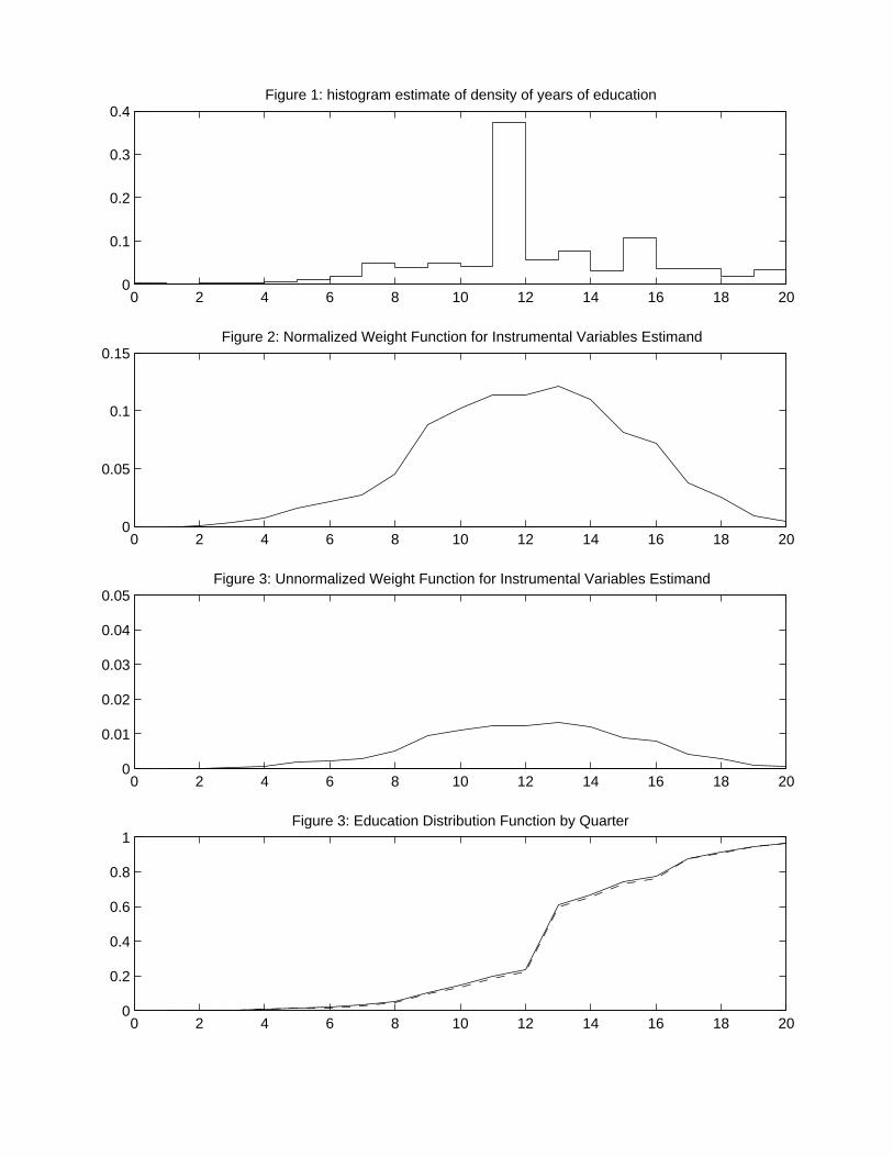
0 2 4 6 8 10 12 14 16 18 200

0.05

0.1

0.15Figure 2: Normalized Weight Function for Instrumental Variables Estimand

0 2 4 6 8 10 12 14 16 18 200

0.01

0.02

0.03

0.04

0.05Figure 3: Unnormalized Weight Function for Instrumental Variables Estimand

0 2 4 6 8 10 12 14 16 18 200

0.2

0.4

0.6

0.8

1Figure 3: Education Distribution Function by Quarter

0 2 4 6 8 10 12 14 16 18 200

0.1

0.2

0.3

0.4Figure 1: histogram estimate of density of years of education