Embed Size (px)
Citation preview

What to Aim for? The Choice of an Inflation Objective when Openness
Matters
March 8, 2016
Richard T. Froyen Alfred V. Guender
Department of Economics Department of Economics and Finance
University of North Carolina University of Canterbury
Chapel Hill, NC 27599-3305 Christchurch
USA New Zealand
Key Words: CPI, Domestic, REX Inflation Targeting, Openness, Inflation-Output Trade-
off.
JEL Code: E3, E5, F3
Abstract:
Inflation targeting countries generally define the inflation objective in terms of the consumer
price index. Studies in the academic literature, however, reach conflicting conclusions
concerning which measure of inflation a central bank should target in a small open economy.
This paper examines the properties of domestic, CPI, and real-exchange- rate-adjusted
(REX) inflation targeting. In one class of open economy New Keynesian models there is an
isomorphism between optimal policy in an open versus closed economy. In the type of
model we consider, where the real exchange rate appears in the Phillips curve, this
isomorphism breaks down; openness matters. REX inflation targeting restores the
isomorphism but this may not be desirable. Instead, under domestic and CPI inflation
targeting the exchange rate channel can be exploited to enhance the effects of monetary
policy. Our results indicate that CPI inflation targeting delivers price stability across the
three inflation objectives and will be desirable to a central bank with a high aversion to
inflation instability. CPI inflation targeting also does a better job of stabilizing the real
exchange rate and interest rate which is an advantage from the standpoint of financial
stability. REX inflation targeting does well in achieving output stability and has an
advantage if demand shocks are predominant. In general, the choice of the inflation objective
affects the trade-offs between policy goals and thus policy choices and outcomes.
E-mail: [email protected]; [email protected]
Corresponding Author: Richard Froyen, Department of Economics, CB 3305, University of North Carolina,
Chapel Hill, NC 27599.
2
By 2006 twenty-five countries mostly small or mid-size open economies had adopted
inflation targeting as a monetary policy strategy. In the wake of the 2007-09 financial crisis
and deep recession, as Svennson (2011) has noted, “no country has so far abandoned inflation
targeting … or even expressed regrets.” Inflation targeting requires the choice of a specific
inflation objective. Inflation targeting countries define the objective in terms of the headline
consumer price index or a modified “core” consumer price index [Svensson (2011)]. This
choice is not surprising as inflation targeting countries tend to be economies where import
inflation is a concern. Performance is typically measured by the central bank’s ability to keep
CPI inflation within a target band or close to a numerical target.1
The academic literature on monetary policy acknowledges that the choice of which
measure of inflation to target is important (Woodford (2011)). Existing studies, however,
even abstracting from the experience of the post-2007 financial and general economic
instability, reached conflicting conclusions about the appropriate target criterion for inflation
in a small open economy. Allsopp, Kara, and Nelson (2006) favor CPI inflation targeting in a
New Keynesian model where exchange rate changes act like supply shocks. In contrast, a
number of influential contributions to the New Keynesian literature (Aoki (2001), Clarida,
Gali, and Gertler (1999, 2001, 2002), Gali and Monacelli (2005), Kirsanova, Leith, and
Wren-Lewis (KLWL) (2006), De Paoli (2009) and others) advocate the stabilization of
domestic rather than CPI inflation.
Models such as Clarida, Gali, and Gertler (1999, 2001, 2002) and Gali and Monacelli
(2005) have the strong implication that optimal policy in an open economy is isomorphic to
policy in a closed economy. This view is reflected in a target rule in an open economy which
is the same as in a closed economy except that the weight on domestic inflation is now
affected by the degree of openness. This isomorphism is a distinctive feature of models where
the output gap is the sole conduit through which monetary policy affects the Phillips curve.
The isomorphism result in an open economy New Keynesian framework has not gone
unchallenged. KLWL (2006) add a terms of trade gap to the objective function of the central
bank after allowing for a wider range of plausible values for the intertemporal elasticity of
consumption and the elasticity of demand. Exchange rate related frictions and an imported
input in production also result in the failure of the isomorphism result. Monacelli (2005)
describes how incomplete-exchange rate pass-through alters the Phillips curve in an open
economy. Domestic inflation is affected by the wedge between the world price (in domestic
1 For a survey, see Walsh (2009).

3
currency) and the home currency price set by importers of the consumption good. In
Monacelli (2013) the existence of an imported intermediate input calls for both real marginal
cost (the inverse of the mark-up) and the terms of trade to be variable.2 Corsetti, Dedola and
Leduc (2011), Engel (2010), Benigno and Benigno (2006), and Clarida, Gali and Gertler
(2002) analyze target rules in a two-country framework where the definition of the central
bank’s objective function depends on factors such as: the values of deep parameters, local
versus producer currency pricing, and cooperative versus non-cooperative policymakers.3
While, as noted above, no central bank has abandoned inflation targeting in the wake of
the financial crisis, there has been an extensive re-examination of the strategy in the academic
literature. One issue is whether consideration of financial stability calls for adding new
objectives to the central bank’s objective function in a flexible inflation targeting regime.4 In
small open economies there is now broader awareness of the threat sudden capital flow
reversals – triggered by external events such as the “lift-off” of US interest rates - pose for
the exchange rate and domestic interest rates. Financial stability in open economies depends
in large degree, though not exclusively, on the volatility of the real exchange rate and interest
rates. An important additional factor that weighs on financial stability is the choice of the
inflation target proper. This is because the inflation objective influences directly the extent to
which the central bank takes account of exchange rate movements and use of its instrument in
implementing monetary policy.
This paper examines the implications of a central bank’s choice of a specific inflation
objective within a flexible inflation targeting strategy. We show that the breakdown or
survival of the isomorphism result hinges on the choice of the inflation objective in the
central bank’s targeting strategy. The choice of the inflation objective affects the form of the
optimal target rule and thus trade-offs between policy goals that confront the policymaker.
Our analysis is conducted within a model with a foundation for an exchange rate channel
in the Phillips curve which does not rely on a particular currency misalignment such as
incomplete exchange rate pass-through or on imports of intermediate inputs. Our Phillips
curve is derived from a setting where domestic firms produce goods for the home market and
exports. Its theoretical basis is an optimizing framework where domestic firms are concerned,
amongst other things, about their competitiveness vis-à-vis foreign firms. As a result, prices
2 Monacelli (2013) argues that consumption openness (under perfect exchange rate pass-through) also accounts
for the breakdown of the isomorphism result.
3 Using a symmetric two-country framework, Bodenstein, Guerrieri, and Kilian (2012) analyze optimal interest
rate responses to headline versus core inflation with endogenous energy prices.
4 See, for examples: Woodford (2012), Smets (2014), Vredin (2015) and Leeper and Nason (2015).
4
set by domestic firms respond to exchange rate fluctuations and changes in the prices charged
by competing foreign firms. If, at the firm level, the pricing is sensitive to movements in the
exchange rate and competitive price pressure from abroad, then, at the aggregate level, such
behavior results in a Phillips curve which features a direct real exchange rate channel. The
standard inflation expectations and the output gap channels are complemented by this real
exchange rate channel.
Following Ball (1999) and Svensson (2000), we trace the implications for monetary
policy of the existence of a real exchange rate channel in the Phillips curve, albeit in a
different modeling framework.5 Our approach to investigate inflation targeting in open
economies is similar in spirit to Svensson. Yet, the current paper emphasizes different aspects
of policymaking in open economies, offering a broader discussion of the factors which affect
the choice of potential inflation targets and giving greater attention to financial stability
concerns. A novel feature of our paper is that it presents tractable optimal target rules that
clearly pin down the role and underscore the importance (relative to the rate of inflation and
the output gap) of the real exchange rate in setting monetary policy. In addition, we analyze
the output-inflation tradeoff under different flexible inflation targeting strategies. Lastly,
there is a more expanded discussion of flexible inflation targeting strategies and the extent to
which their performance is influenced by the central bank’s relative aversion to inflation
variability and the sources of uncertainty.
We examine three flexible inflation targeting strategies: domestic inflation targeting, CPI
inflation targeting, and real-exchange rate-adjusted (REX) inflation targeting. REX inflation
is defined as domestic inflation purged of the effects of real exchange rate changes.6 For each
of these strategies we derive the optimal target rule and analyze the ways in which the rule
differs from the rule in the canonical closed-economy New Keynesian model.
For CPI or domestic inflation targeting, our analysis leads to several conclusions. First,
the real exchange rate plays a much more important role in the design of target rules than in
5 Ball’s model is completely backward-looking while Svensson’s features both backward-and forward-looking
elements. In Svensson’s framework domestic inflation in the Phillips curve is pre-determined so as to allow for
a two-period lag of the effect of monetary policy on domestic inflation. This lag pattern is absent in our
modelling framework. The real exchange rate channel in Svensson’s Phillips curve is more subdued than in our
version of the Phillips curve. Domestic inflation in period t+2 is affected by the expected change in the real
exchange rate from period t+1 to period t+2. This expectation is formed in period t.
6 The definition of REX inflation differs from Ball’s definition of long-run inflation in one important respect.
Ball’s measure relates the level of the lagged real exchange rate to overall inflation while our definition of REX
inflation represents domestic inflation adjusted for the degree of supply openness and the change in the real
exchange rate. Unlike Ball’s, our definition thus has the natural advantage of being able to distinguish between
the REX price level ( ) and the REX inflation rate (
). Froyen and Guender
(2014) provides a discussion of the importance of choosing a REX price level target in delegating the conduct
of monetary policy to a conservative central banker in an open economy.

5
most previous frameworks. Second, the isomorphism result in the earlier literature breaks
down if there is a separate exchange rate channel in the Phillips curve. Third, the exchange
rate channel for policy improves the inflation- output tradeoff in the presence of cost-push
shocks. As a consequence of this improved trade-off, more weight is put on inflation
stabilization in the target rule.
REX inflation targeting restores the isomorphism to policy in the closed economy. It
becomes more desirable as the consequences of openness just set out become undesirable. As
the incidence of demand-side shocks increases relative to cost push shocks, for example, the
ease with which these shocks are offset in the closed economy favors REX inflation
targeting. REX inflation targeting also becomes more desirable if the central bank puts more
weight on output stabilization in the objective function; openness, by improving the inflation-
output-trade-off, raises the opportunity cost of gains in output stability.
A central bank’s innate aversion to inflation relative to output variability plays a decisive
role in the choice of which inflation rate to target. Even if demand-side shocks are
substantially more volatile than cost-push shocks, an optimizing central bank that places
greater emphasis on price stability chooses CPI inflation targeting over domestic or REX
inflation targeting. One attractive feature of CPI inflation targeting is that it also ensures
stability of domestic and REX inflation while the reverse does not hold. Additionally, CPI
inflation targeting is superior from the standpoint of stabilizing the real exchange rate and
domestic interest rate, an advantage for the maintenance of financial stability.
The paper is organized as follows. In Section 2 we derive an open-economy Phillips
curve and incorporate it into a small open-economy New Keynesian model. Section 3
discusses the three flexible inflation targeting strategies. A performance analysis is carried
out and commented on in Section 4. Section 5 concludes.
2. The Building Blocks of the Model
A. An Open Economy Phillips Curve
The central building block for our open economy Phillips curve is the firm’s pricing
equation. Recent evidence from surveys [Greenslade and Parker (2012) and Parker (2012)] as
well as from micro data [Bunn and Ellis (2012a), (2012b)] indicates wide divergence in
pricing behavior within and across sectors of the economy. These studies cast doubt on
whether any one theory can adequately capture all the important features of firm pricing. In
particular the popular specification of Calvo (1983) pricing supplemented by “rule of thumb”

6
indexation appears to describe actual pricing behavior of only a small minority of firms.
Given the heterogeneity of firm pricing behavior, any aggregate price setting equation will be
an approximation aimed at capturing some central features of the process.
The pricing framework here emphasizes three elements, each of which receives support
from this survey evidence for the United Kingdom [Greenslade and Parker (2012)] and for
New Zealand {Parker (2012)]. First, we assume firms follow mark-up pricing influenced by
the benchmark prices of competing domestic firms. Second, we assume that there is price
stickiness due to menu costs. Menu costs include not just the physical costs of price changes
but are also the result of implicit and explicit contracts as well as coordination problems.
Finally, in the open economy the firm is concerned with competitiveness at home and abroad.
Thus the firm responds to exchange rate induced changes in the terms of trade.7
We model these elements of optimal price setting within an extension of Rotemberg’s
(1982) quadratic cost adjustment model of monopolistically competitive firms. In our open-
economy version of the model an optimizing firm sets the price of output so that the overall
cost function which consists of three separate components is minimized. The objective
function of the typical firm j is:
∑ [
]
(1)
where:
( )tjΩ = the total cost of firm j at time t
( )tp j = the price of the good produced by firm j at time t
= the optimal mark-up price for firm j
( ) ( ) ft t t tq j p s p j = firm-specific terms of trade
= the price of the foreign good in foreign currency
= the nominal exchange rate (units of domestic currency per unit of foreign
currency)
= the constant discount factor
7 In New Zealand, competitors’ price changes—both increases and decreases-- were deemed to be the most
important factor in an exporting firm’s decision to change price. Exchange rate changes were found to be an
important or very important factor in determining price changes by more than 70 percent of exporters among the
survey respondents in the United Kingdom. Support for the importance of exchange rate changes as an influence
on price setting in the United Kingdom is also provided by Bunn and Ellis (2012a, 2012b).

7
c = the parameter that measures the costs of changing prices relative to the costs of
deviating from the optimal mark-up price
= the parameter that measures the costs of changes in the firm’s terms of trade
relative to the costs of deviating from the optimal mark-up price
tE = the expectations operator conditional on information available at time t.
The first term within the brackets is the cost of being away from the optimal mark-up
on cost, the price that the firm would charge in the absence of menu costs and foreign
competition. This price, the specification of which is explained below, is denoted p(j)*. Menu
costs are represented by the second term in brackets.
In an open economy, as explained previously, firms are concerned about
competitiveness abroad as well as at home. Define the terms of trade (or real exchange rate)
as the domestic currency price of foreign output relative to the price of domestic output. The
firm-specific terms of trade measure a representative firm’s price competitiveness vis-à-vis
foreign competition. To avoid changes in its terms of trade caused by sudden exchange rate
movements or foreign price movements both of which are beyond its control, the firm is
required to alter its price. Menu costs make this costly.
The firm sets the price of its output in domestic currency. Taking the first-order
condition and running the expectations operator through it, we can characterize the
relationship between past, current, and future prices as well as the current and expected
change in the terms of trade as:8
)
(2)
From equation (2) it is evident that the current and the expected change in the firm-specific
terms of trade matter in setting the price at time t. The greater a - the relative weight on the
change in the terms of trade in the total cost function - compared to c, the relative weight on
costly price changes, the more current and expected changes in the terms of trade factor in the
decision to change the price in the current period.
Next, consider the formation of the firm’s optimal mark-up price:
8 From the definition of the firm-specific terms of trade and the fact that the firm cannot influence the price set
by foreign competitors or the nominal exchange rate it follows that

8
+ (3)
where all variables are as previously defined. In addition:
tp = the price charged by competing firms at time t
ty( j ) = output produced (relative to potential) by firm j
t( j ) = a stochastic disturbance.
Under imperfect competition, is a mark-up over marginal cost. But marginal
cost and real output are positively related.9
Therefore we replace marginal cost with the
output gap in (3). To capture the idea of a time-varying mark-up factor, we model it as a
random element that enters into the process of setting the optimal mark-up price. The
other factor that influences the firm’s optimal mark-up price is the benchmark price set by
competing firms. This price, denoted by tp , equals the aggregate domestic price level tp .
Substituting equation (3) into (2) and aggregating over all firms yields equation (4),
an open-economy Phillips curve where, in addition to the output gap and expected domestic
inflation, the current and expected change in the real exchange rate affect current domestic
inflation.10
(4)
where
Compared to the standard closed-economy Phillips curve, the open-economy
representation features a more expansive expectations channel that operates through expected
changes in the real exchange rate. In addition, the current period change in the real exchange
rate exerts a direct effect on domestic inflation.
9 Equation (3) is the same as the one proposed by Roberts (1995). Within a general equilibrium framework, the
co-movement between marginal cost and economic activity can be established by combining the labor supply
and demand relations with the market clearing condition in the goods market. On this point see Clarida, Gali,
and Gertler (2001, 2002) or Gali and Monacelli (2005).
10 For simplicity there is no distinction between the terms of trade and the real exchange rate.

9
B. Model for a Small Open Economy
The complete model for a small open economy consists of four equations:
t t t 1 t t t 1 t t 1 t tπ βE π κy b(q q ) βb(E q q ) u
(4)
CPI f ft t t 1 1 t t t 1 2 t t t 1 3 t t t 1 ty E y a (R E π ) a (q E q ) a ( y E y ) v
(5)
t
f ft t t 1 t t 1 t t 1 t tR E π R E π E q q ε
(6)
CPIt t tπ π γΔq
(7)
t the rate of domestic inflation
CPI
1ttE the expected rate of CPI inflation
tq the real exchange rate
ty = the output gap
tR the nominal rate of interest (policy instrument)
f
tR the foreign nominal rate of interest
f
1ttE the expected foreign rate of inflation
f
ty = the foreign output gap
Lower case variables represent logarithms. All parameters are positive. The discount factor
is less than or equal to one.
Equation (4) is the open-economy Phillips curve. Equation (5) is the open economy
IS relation that features a real interest rate and real exchange rate channel. A foreign output
shock and an idiosyncratic shock affect demand for domestic output.11
Equation (6) is the
linearized uncovered interest rate parity (UIP) condition: apart from a stochastic risk
premium ( ) agents are assumed to trade in a frictionless international bond market. More
formally, the stochastic disturbances are modeled as follows: 12
We treat all foreign variables as exogenous random variables that are independent of each
other. Finally, equation (7) describes the relationship between the CPI inflation rate, the
11 The derivation of the forward-looking IS relation from microeconomic foundations is explained in Guender
(2006). A separate appendix, available from the authors, shows how the shocks that appear in the IS relation can
be motivated.
12 The property that all shocks are white noise follows Woodford (1999a). Its purpose is to show that gradual
adjustment of the output gap, the rate of inflation, etc. are not exclusively tied to the presence of autocorrelated
disturbances in the model.

10
domestic inflation rate, the real exchange rate, and consumption openness (γ) under perfect
exchange rate pass-through.
3. Targeting Different Measures of Inflation
Woodford (2011, p.802) recognizes that “the question as to which measure of
inflation should be targeted by a central bank is an important practical question for the theory
of monetary policy.” We conceive of this question of a particular inflation target being
confronted by the central bank (or government) of an open economy such as Australia, New
Zealand or Switzerland. What criteria should guide this choice and, more generally, that of an
inflation targeting regime? The literature distinguishes two approaches. One emphasizes a
welfare-theoretic approach to determine the central bank’s target criterion while the other is a
“simple representation of conventional central bank objectives (Woodford (2011, p.728).”
Under the welfare-theoretic target criterion, the central bank minimizes a loss
(objective) function given by an approximation to a representative household’s utility
function. A welfare-based criterion has a strong claim to legitimacy in the optimal policy
literature. Such a loss function is, however, model-specific and depends critically on the
specification of the consumer’s utility function and the values chosen for the elasticity of
substitution, elasticity of demand, and other factors.13,14
We adopt the less formal approach in which the central bank decides on (or is
assigned) a menu of flexible inflation targeting strategies, each containing the output gap as
well as an inflation measure to target. Within the model we have set out, the central bank
traces out the implications of adopting the alternative inflation targets. This approach allows
us to focus on the implications of the choice of an inflation target for: the optimal target rule,
the output-inflation variability trade-off, and the effects of various shocks in the model.
How far does this take us away from a welfare-based measure? Woodford (2011,
p.776) concludes “in a broad range of models” maximizing the expected utility of a
representative household is consistent with a central bank’s objective of minimizing
fluctuations in some measure of inflation and the output gap. Thus the welfare theoretic
approach and the more pragmatic representation of conventional central bank objectives are
broadly consistent in many contexts. Also relevant is Woodford’s view that “[a]s a practical
13 Kirsanova et al (2006) show that relaxing the assumptions of unitary elasticity of demand and intertemporal
substitution results in a far more complex welfare criterion than proposed by Gali and Monacelli (2005).
14 Exclusive reliance on utility-based welfare metrics has drawn some criticism. Clarida, Gali and Gertler
(1999, p.1688) conclude that the micro-founded DSGE New Keynesian approach "could be misleading as a
guide to welfare analysis because of its highly stylized microeconomic underpinnings." Sims (2012) echoes
their concerns citing the implausibility of the microeconomic foundations of these DSGE models.

11
matter, then, it is important to formulate recommendations for relatively simple target
criteria, that while not expected to be fully optimal, it is nonetheless an approximate optimal
policy to a reasonable extent (2011, p. 822).”
A final point to consider before proceeding to the policy regimes we examine is
whether in light of the financial crisis a financial stability objective should be included in the
central bank objective function. There are different views on the question as explained, for
example, in Smets (2014). Woodford (2012) argues that a flexible inflation targeting regime
should be expanded to include a financial stability objective which is then included in the
optimal target rule for monetary policy. Curdia and Woodford (2011) develop a model that
supports such an expansion based on the presence of frictions in the financial intermediation
process. Smets (2014, p. 263) argues for a less direct linkage where the objective function is
not modified but where the “monetary policy authorities should also keep an eye on financial
stability.”
As noted in the introduction, for small open economies the real exchange rate and the
interest rate are important transmission channels for financial instability. Thus the question of
expanding an inflation targeting framework to incorporate financial instability brings us to
the question of whether these variables should enter the central bank loss function and
targeting rules. Blanchard et. al. (2010), for example, suggest that “central banks in small
open economies should openly recognize that exchange rate stability is part of their objective
function.” The question addressed here is the choice of an inflation target. Rather than
specify a weight for exchange rate stability in the loss function, we take the approach
suggested by Smets (2014) and assume that while the targeting regime consists of only
squared deviations of the inflation measure and the output gap, the policymaker monitors the
behavior of the real exchange rate and interest rate. The volatility of these variables is shown
to depend on the choice of the inflation measure to target. It will also be seen that even if the
real exchange rate is not incorporated into the central bank loss function, it will appear in the
optimal target rule for two of our inflation measures.
Thus, in what follows we consider three flexible targeting regimes. As just explained,
in the simple version used here flexible inflation targeting is where the objective function
consists of squared deviations of the output gap and the rate of inflation the central bank
targets. The three inflation targets are: domestic inflation, exchange-rate adjusted inflation,
and CPI inflation. At the core of each regime is a tractable optimal target rule that prescribes
how the target variables and other relevant endogenous variables interact to ensure that the
objective function is minimized. The central bank uses discretion in setting optimal policy.

12
A. Targeting Domestic Inflation
In the first strategy inflation is defined in terms of changes in the level of domestic
prices. The explicit objective function that the central bank minimizes is given by:
∑
(8)
is the discount rate and represents the relative weight the policymaker attaches to the
squared deviations of the rate of domestic inflation from target.15
To illustrate how optimal policy in the open economy is determined, it is helpful at the
outset to reduce the dimension of the problem to one involving only two constraints. Two
steps need to be taken. First, substitute for the rate of CPI inflation in equation (5). Second,
substitute the UIP condition into the IS equation. The problem can then be expressed as:
∑
s. t
t t t t t t t t t t
π βE π κy b q q βb E q q u1 1 1
( ) ( )
(9)
and
(
)
(
)
The resulting target rule under flexible domestic inflation targeting is:16
(
)
(10)
( ) ( )
The open economy target rule is more complex than in the canonical closed-economy
New Keynesian model. First, even though it does not appear in the objective function, the
real exchange rate appears in the target rule alongside the target variables and The real
exchange rate provides essential information. Second, both Phillips curve and IS parameters
as well as the discount factor determine the relative weights on the rate of domestic inflation
15 The target for the output gap and the rate of inflation is zero, respectively.
16 A step-by-step derivation of all target rules and an explanation of the solution technique employed to
determine the forward-looking expectations of inflation, output, and the real exchange rate appear in the
appendix which is available upon request from the authors. The coefficients are the respective
coefficient on the lagged real exchange rate in the putative solution for and

13
and the real exchange rate. The size of these weights depends on the strength of the
(expected) real interest rate and exchange rate channel on the demand side and the sensitivity
of domestic inflation to the output gap and changes in the real exchange rate on the supply
side. The difference between the target rule in a closed economy and the target rule in an
open economy is due to the existence of the exchange rate channel in the Phillips curve. If b
= 0, then and the open-economy target rule reverts to its closed-economy
counterpart. Equation (10) can be combined with the Phillips curve, the IS relation and the
UIP condition to generate solutions for the endogenous variables and their variances.
B. Targeting “R(eal)-EX(change)-Rate-Adjusted” Inflation
As mentioned in the introduction, several contributions to the literature argue that
optimal policy in an open economy is isomorphic to policy in a closed economy. Our aim in
this section is to show that by choosing an alternative target variable for inflation an open-
economy target rule can be made to look exactly like its closed-economy counterpart. This
alternative target variable is domestic inflation stripped of the effects of changes in the real
exchange rate.
The preceding section showed that the existence of a real exchange rate channel in the
Phillips curve is instrumental in shaping the target rule for an open economy. Both the
current and expected change in the real exchange rate appear on the right-hand side of the
Phillips curve, which is shown again for convenience below.
t t t 1 t t t 1 t t 1 t tπ βE π κy b(q q ) βb(E q q ) u
(4)
The Phillips curve can be rewritten as
t t t t t t t t t tπ b(q q ) β(E π b(E q q )) κy u
1 1 1
Defining
REXt t t tπ π b(q q )
1 (11)
as the domestic rate of inflation purged of the real exchange rate effect allows us to rewrite
the original open-economy Phillips curve as
REX REXt t t t tπ βE π κy u
1 (12)
Written in this form, equation (12) looks like the original Phillips curve. The only difference
between equation (4) and equation (12) pertains to the definition of the rate inflation.

14
The remaining two equations of the model can be rewritten in terms of the real-
exchange-rate-adjusted rate of inflation:
REX f ft t t 1 1 t t t 1 1 2 t t 1 t 3 t t t 1 ty E y a (R E π ) (a (b γ ) a )(E q q ) a ( y E y ) v
(13)
REX f
t t t 1 t t 1 t t 1 t t
ftR E π R E π (1 b)(E q q ) ε
(14)
The last change is a modification of the objective function of the policymaker. The
target variable for inflation is now the real-exchange-rate-adjusted rate of inflation.
After substitution of equation (14) into equation (13) to eliminate the real exchange
rate, the optimization problem of the policymaker can be stated as:
2 2
0
1
2
REXt t t
i REXt t i t i
y ,π ,Ri
min E [ β [ y μπ ]] (15)
s. t.
REX REXt t t t tπ βE π κy u
1
and
REX REX f f f f1 2t t t 1 1 t t t 1 t t t 1 t t t 1 t 3 t t t 1 t
(a (b γ ) a )y E y a (R E π ) (R E π R E π ε ) a ( y E y ) v
1 b
Solving the optimization problem yields the target rule under REX inflation targeting:
REX
t ty μκπ 0 (16)
As in the closed-economy model, only the Phillips curve parameter κ appears in the target
rule. Demand-side parameters have no role to play. Combining equation (16) with equations
(12) – (14) yields the solutions for the endogenous variables and the policy instrument.
C. Targeting CPI Inflation
If the focus of policy rests on CPI inflation, then the policymaker minimizes
i 2 CPI 2
t t i t i
i 0
1E [ [ y ]]
2
(17)
subject to the constraint represented by the model economy. After rewriting the structure of
the economy in terms of the CPI inflation rate, we can restate the policy objective as:
CPIt t t
i CPIt t i t i
y ,π ,qi
min E [ β [ y μπ ]]
2 2
0
1
2
subject to (18)
CPI CPIt t t 1 t t t 1 t t 1 tπ βE π κy (1 β)(γ b)q (γ b)q β(γ b)E q u

15
and
f f f ft t t 1 1 t t t 1 t 1 2 t t 1 t 3 t t t 1 ty E y a (R E π ε ) (a (1 γ ) a )(E q q ) a ( y E y ) v
(19)
Combining the first-order conditions of the optimization problem leads to the following target
rule:17
(
)
(20)
( ) ( )
As with the target rule under domestic inflation targeting, the real exchange rate appears in
the target rule in addition to the target variables proper. Again, the level of the real exchange
rate provides essential information that is contained neither in the rate of CPI inflation nor the
output gap. Although the target rule under CPI inflation targeting looks similar to the target
rule under domestic inflation targeting, there is one fundamental difference between the two
rules. Even if the real exchange rate channel in the Phillips curve is shut off, i.e. b = 0, the
target rule under CPI inflation targeting does not revert to the closed-economy target rule in
the canonical New Keynesian model. Setting b = 0 results neither in nor in reducing
the coefficient on the real exchange rate to zero. The relative weight on the CPI inflation rate
and the real exchange rate, respectively, merely decreases in size. By definition, the CPI
inflation rate depends in part on the degree of openness multiplied by a change in the real
exchange rate. Thus, if the policymaker changes the policy instrument in response to a
demand-side shock, the real exchange rate changes, which in turn filters through to the CPI
inflation rate. Attempting to prevent the output gap from changing does not work in the
present case because the rate of CPI inflation is directly affected by changes in the real
exchange rate.
Solutions for the endogenous variables and the policy instrument and their variances
are obtained by combining equation (20) with equations (18) and (19).
4. Assessing the Performance of the Flexible Inflation Targeting Strategies
The previous section establishes that, depending on the choice of an inflation objective,
optimal monetary policy in an open economy can but need not be isomorphic to that of a
closed economy. While informative, the isomorphism result by itself says very little about the
17 The coefficients are the respective coefficient on the lagged real exchange rate in the putative
solution for and
16
relative merits of flexible domestic, CPI, and REX inflation targeting. This section therefore
carries out two tests to evaluate the performance of the three monetary policy strategies. The
first test assesses the role of a central bank’s innate aversion to inflation variability in ranking
the flexible inflation targeting regimes by loss score. It further compares the variability of the
output gap across the different inflation targeting regimes and examines the extent to which a
particular choice for the inflation objective achieves price stability across the board.18
Consideration is also given to the behavior of the real exchange rate and the policy
instrument. The second test assesses the inflation-output gap tradeoffs under each of the three
flexible inflation targeting regimes. Prior to these assessments we examine the target rules
underlying the three inflation targeting strategies. A comparison of the target rules allows us
to make conjectures about the extent to which the output gap and the real exchange rate
fluctuate across the flexible inflation targeting regimes, conjectures that receive strong
support in the numerical assessments that follow.
A. The Three Target Rules
A central focus of the current paper is to highlight the differences among regime-
specific target rules. Table 1A presents the target rule for each of the three flexible inflation
targeting strategies. Consider the weights the central bank attaches to the inflation rate and
the real exchange rate relative to the output gap under domestic and CPI inflation targeting.
The coefficients and play an important role in determining the size of these
weights. The four coefficients describe the potency of the monetary transmission channels in
the Phillips curve ( and the IS relation ( under the two monetary policy strategies.
Both consumption openness ( ) and supply-side openness ( ) matter for the size of
while only the latter directly affects the size of . As a result > the real exchange rate
channel in the Phillips curve is more potent under CPI than under domestic inflation
targeting. At the same time = , which suggests that the choice of inflation objective has
no implications for the strength of the monetary transmission channels on the demand side.19
18 Arguably, price stability goes beyond keeping a given measure of inflation low and stable. In New Zealand,
for instance, price stability is defined not solely in terms of CPI inflation but in terms of changes in the general
level of prices. This clearly indicates that changes in other price indices figure in the overall assessment of
flexible CPI inflation targeting (Monetary Policy and the New Zealand Financial System (1992), p. 35).
19 As analytical solutions do not exist under domestic and CPI inflation targeting these results are established
by solving the models numerically. The numerical solutions establish, for instance, that | | | |. The effect
of the current real exchange rate on expected CPI inflation is greater than on expected domestic inflation. More
details on the numerical solution procedure are given in the appendix.
17
With > the relative weight on inflation under CPI inflation targeting is greater
than the relative weight on inflation under domestic inflation targeting. Also, the relative
weight on the real exchange rate in the CPI inflation target rule is greater than its counterpart
in the domestic inflation target rule. Both consumption and supply openness affect the size of
the numerator of the coefficient on in the CPI inflation target rule but not in the domestic
inflation target rule where only supply openness matters.
In general, the size of the relative weight on inflation and the real exchange rate in the
respective target rule reflects the importance of these two variables vis-à-vis the output gap in
the setting of policy under the three regimes. In the case of flexible inflation targeting where
both the inflation and the output gap objective are deemed important, the size of the relative
weights in the target rules should convey information about the variability of those variables
that explicitly or implicitly figure in all three target rules.20
According to Table 1A, the
relative weights on inflation and the real exchange rate are largest under CPI inflation
targeting but smallest under REX inflation targeting. This suggests the following conjectures:
Conjecture 1:
The output gap is most stable under REX inflation targeting.
Conjecture 2:
Fluctuations in the real exchange rate should be lowest under CPI inflation targeting but most
pronounced under REX inflation targeting where the relative weight on the real exchange rate
is zero.
To assess the plausibility of these conjectures, we use a numerical solution procedure
with the following plausible parameter values:
The choice of parameter values is explained in the note below Table 1.
For the computation of the variances of endogenous variables in Section B we assume that all
disturbances are independent white noise processes with unit variance.
Using the above parameter values, we calculate the relative weights on the respective
rate of inflation and the real exchange rate in the three target rules. These relative weights
appear in Table 1B. Each horizontal line is based on a different value of the relative inflation
aversion parameter .The entries confirm that the relative weight on inflation is largest under
CPI inflation targeting and smallest under REX inflation targeting. One feature of flexible
CPI inflation targeting is that the relative weight the central bank attaches to the CPI inflation
rate in the target rule roughly corresponds to its relative aversion to inflation variability in the
20 To give precise meaning to the concept of “importance”, we let µ take on values 1, 4, and 8.

18
objective function. Also, under flexible CPI inflation targeting, the relative weight on the real
exchange rate is considerably higher than under domestic inflation targeting.
B. Variability of the Model Variables Across the Three Regimes
The results of the comparison of the three targeting strategies are presented in Tables 2,
3, and 4. Table 2 shows the results for the case when the policymaker is equally concerned
about inflation variability and output gap variability while Tables 3 and 4 report the
results for the case where the policymaker’s concern about inflation variability increasingly
outweighs the concern about output gap variability, i.e. and , respectively.
Let us begin by considering the information contained in section A of Tables 2 and 3.
The loss scores for the three inflation targeting regimes appear in bold-face as diagonal
entries. Off-diagonal entries show how losses change if the variance of one of the two
alternative measures of inflation takes the place of the variance of the inflation rate being
targeted in the loss function. Inspection of the diagonal elements of the two tables reveals a
striking contrast. The ranking of the three inflation targeting strategies by loss score is
reversed as the central bank’s emphasis shifts from equal concern about inflation and output
gap variability towards greater concern about inflation stability. Placing greater emphasis on
inflation stability clearly favors CPI targeting over domestic and particularly REX inflation
targeting which dominates the other two strategies for Losses under CPI inflation
targeting are also fairly compact but far less so for domestic and REX inflation targeting as
the variance of CPI inflation increases markedly under both regimes.
A second result is that a CPI inflation target produces the lowest variance for all three
inflation measures. Indeed the variance of REX inflation is smaller than the variance of CPI
inflation itself if and the central bank chooses a CPI inflation objective; the variability
of domestic inflation is only slightly above that of CPI inflation. In contrast, domestic and
especially REX inflation targeting results in substantial variability of CPI inflation. Putting
greater emphasis on inflation control in the objective function ( ) leads to a massive
drop in the variance of CPI inflation under CPI inflation targeting – more than threefold- but
only moderate (domestic inflation targeting) or slight (REX inflation) decreases in the
variance of the chosen target under the alternative targeting strategies.
CPI inflation targeting has the drawback that it leads to pronounced fluctuations in the
output gap compared to the other two strategies. This is evidenced by the low variability of
the output gap under domestic inflation targeting (0.064) and particularly under REX

19
inflation targeting (0.0098) relative to CPI inflation targeting (0.6149) in the case where
(Confirmation of conjecture 1). With a relatively low relative weight on the inflation
rate (µ=1), the central bank’s concern with stabilization of the output gap makes REX
inflation targeting the preferred strategy. Moreover, REX inflation targeting has the
advantage that the output gap and REX inflation are sensitive only to cost-push disturbances.
Demand-side disturbances can be completely offset by manipulating the policy instrument.
Financial stability concerns are important in assessing the stance of monetary policy.
Central banks wish to avoid contributing to erratic swings in asset prices that have the
potential to cause upheaval in financial markets and the wider economy. How do the three
inflation targeting regimes affect the variability of the real exchange rate and the policy
instrument? Inspection of the lower right half of Tables 2 and 3 confirms conjecture 2: CPI
inflation targeting stabilizes the real exchange rate much better than the alternative targeting
strategies. CPI inflation targeting also makes for less variation of the nominal interest rate.
The results described above do not change markedly if the central bank places even
greater relative emphasis on inflation stability . According to Table 4, only two minor
modifications must be made to our assessment of the targeting strategies. Both changes
concern the relative standing of domestic inflation targeting: of the three strategies it is now
best at controlling the variability of domestic inflation but worst at managing the variability
of the real exchange rate.21
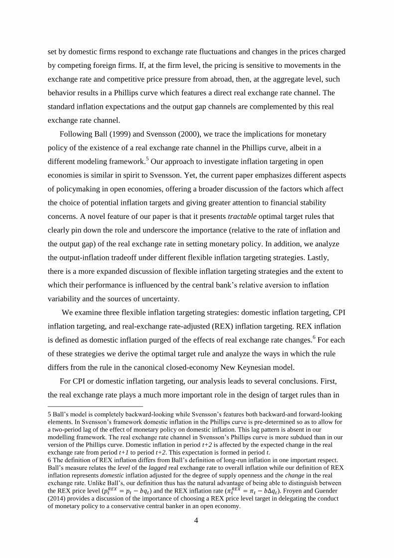
C. Policy Frontiers and Inflation-Output Variability Tradeoffs
Additional evidence on the performance of the three flexible inflation targeting
strategies can be gleaned by considering the shape and location of policy frontiers which
describe the inflation-output variability tradeoffs under each regime. Figure 1 shows the
policy frontiers under CPI inflation, domestic, and REX inflation targeting.22
In addition to
the policy frontier for the targeted inflation measure, each segment of the figure shows the
frontier for the non-targeted inflation measures. This reflects our interest in the degree to
which each strategy provides general price stability.
It is apparent that the three targeting strategies produce vastly different inflation-
output variability tradeoffs. In Figure 1C, under REX inflation targeting, the inflation-output
21 The ranking of policy regimes under discretion is not altered by considering optimal policy under
commitment from a timeless perspective as in Woodford (1999a). In general, the output gap becomes more
variable and each rate of inflation less variable under commitment.
22 For each strategy, the inflation-output variability frontier is constructed by varying the relative weight on the
rate of inflation in the objective function. μ takes on values 1, 4, and 8.

20
variability tradeoffs are compact. There is not much variation in fluctuations of the output
gap and the rate of inflation (no matter how inflation is measured). There are, however,
dramatic differences in the loci of the variability tradeoffs. The policy frontier along which
CPI inflation variability is traded off for output gap variability under REX inflation targeting
is a considerable distance to the right of (and hence inferior to) the policy frontiers that
govern the tradeoff between output gap and REX inflation variability and the tradeoff
between output gap and domestic inflation variability. Figures 1A and 1B illustrate that CPI
inflation and especially domestic inflation targeting give rise to far wider inflation-output
variability tradeoffs. These observations admit a simple interpretation: the central bank’s
relative aversion to inflation variability is of less consequence for the variability of the
output gap and all three measures of inflation if it targets REX inflation.
In two of the three cases considered the inflation rate targeted traces out the most
preferred policy frontier, i.e. the one closest to the origin. Figure 1A depicts the three policy
frontiers under CPI targeting. The one which describes the tradeoff between the variability of
CPI inflation and the output gap lies to the left of those based on REX or domestic inflation.
In Figure 1B we find a similar result: under domestic inflation targeting, the tradeoff between
domestic inflation variability and output gap variability occurs to the left of the policy
frontiers based on REX inflation or CPI inflation. Figure 1C illustrates a contrary example.
When price stability is of great or medium concern, REX inflation targeting produces a
variability tradeoff between itself and the output gap that lies above the variability tradeoff
between domestic inflation and the output gap.
A striking feature that can be seen from comparing the three segments of Figure 1 is
that CPI inflation targeting provides relatively low inflation variability across all three
inflation measures. Each of the other strategies produces relatively poor performance for CPI
inflation. This results from the fact that these other strategies produce very high variance in
the real exchange rate with adverse effects on the variance of CPI inflation.
Figure 1D provides more information on the behavior of the real exchange rate as
well as that of the policy instrument under the three targeting strategies. In general, greater
emphasis on inflation leads to greater variability in both the real exchange rate and the policy
instrument as optimal policy becomes more aggressive. From the standpoint of financial
stability, however, it can be seen from the figure that both are least volatile under CPI
inflation targeting for all levels of inflation aversion.

21
D. How Sensitive is the Ranking to the Sources of Shocks?
A central result of Clarida, Gali and Gertler’s (1999) analysis of monetary policy in the
closed economy is that “[t]he optimal policy calls for adjusting the interest rate to perfectly
offset demand shocks ….Demand shocks do not force a short-run trade-off between output
and inflation.” This result does not necessarily carry over to the type of open-economy
model considered here but depends on the central bank’s inflation objective. As in Poole
(1970), the ranking of alternative strategies in the model will depend on the relative
variability of the shocks faced by the policymaker. Under domestic or CPI inflation
targeting, the policymaker confronted with demand-side shocks faces a tradeoff between
stabilizing inflation and the output gap. The isomorphism between optimal monetary policy
in the open and closed economy breaks down. REX inflation targeting restores the
isomorphism. The Clarida, Gali and Gertler (1999) result for demand-side shocks holds
under this targeting procedure.
To see how the origin and variability of shocks affects the ranking of the three
targeting procedures, we modify the original set-up by increasing the variance of each
demand-side disturbance from one to four while the variance of the cost-push shock is kept at
one. Table 5 presents the findings with this modification when the central bank is equally
concerned about inflation and output gap variability (μ=1). Table 6 shows findings for
substantially greater aversion to inflation variability (μ=8).
First, compare the loss scores in the top panels of Tables 5 and 6 to those in Tables 2
and 4. From a loss minimizing perspective, a central bank with a relatively low aversion to
inflation variability (μ=1) does best under REX inflation targeting. The advantage of this
strategy increases if shocks to the demand side of the economy are far more variable than the
cost-push shock (Table 5 compared to Table 2). As the demand-side shocks become more
variable, the loss score for REX inflation targeting is unchanged while the loss score for the
other two strategies rises. Comparison of Tables 4 and 6 shows, however, that a highly
inflation-averse central bank (μ=8) would still choose CPI inflation targeting with highly
variable demand-side shocks albeit by a smaller margin.
Thus, as expected, more variability of demand-side shocks favors REX inflation
targeting; under this strategy these shocks are perfectly offset by adjusting the interest rate.
CPI inflation targeting is still attractive as can be seen from the rankings of the three
strategies if performance is measured by minimizing the variances of each of the inflation
measures we consider. Moreover, while the variance of the real exchange rate and nominal

22
interest rate increase for all strategies as demand shocks become more variable, CPI inflation
targeting still produces the lowest variance for both. These results hold for either µ=1 or µ=8.
To summarize, an increase in the variability of demand-side shocks relative to cost-
push shocks increases the desirability of REX inflation targeting relative to the other two
strategies. Even so, CPI inflation targeting retains its advantage in providing low inflation
variability by all measures and results in lower variability of the real exchange rate and policy
instrument.23
5. Conclusion
This paper considers the choice of an inflation objective in a New Keynesian open
economy model which has a direct exchange rate channel in the Phillips curve. In the model
this channel results from the fact that producers care about the real exchange rate in setting
prices. There are other rationales for such a real exchange rate channel in models such as
those of Ball (1999), Svensson (2000) and Froyen and Guender (2007). With a direct
exchange rate channel in the Phillips curve the transmission mechanism of monetary policy
no longer works exclusively through the output gap. Instead it relies as well on the real
exchange rate to bring about changes in the rate of inflation.
A more expansive transmission mechanism affects optimal central bank policy. If the
CPI or domestic rate of inflation is the inflation objective, the current framework has policy
implications that differ sharply from models such as those of Clarida, Gali and Gertler (2001,
2002) and Gali and Monacelli (2005) which do not provide for a direct exchange rate
channel in the Phillips curve. In their open-economy models optimal monetary policy is
isomorphic to that in the closed-economy counterpart. With a direct exchange rate channel,
the isomorphism breaks down. The difference in optimal policies is most easily seen in the
specification of the target rules (Table1). With a direct exchange rate channel in the Phillips
curve, the real exchange rate appears as an essential element in the target rule. In addition,
characteristics of the demand-side of the economy influence the relative weights the central
bank places on the components of the target rule. Demand-side disturbances can no longer be
offset by a mere adjustment of the policy instrument; the response to all disturbances
depends on the central bank’s relative aversion to inflation variability.
23 We have also checked the sensitivity of the results reported to a change in the size of b, a key parameter. If
supply side openness increases from 0.1 to 0.25, domestic and CPI inflation targeting achieve lower inflation
variability at the expense of higher output gap variability. Losses increase somewhat under domestic and CPI
inflation targeting but remain invariant under REX inflation targeting. The inflation-output gap variability trade-
off frontiers shift up and to the left but the general shape of the frontiers remains similar to those in Figure 1.

23
We consider a real-exchange-rate-adjusted (REX) inflation targeting regime that
restores the isomorphism with policy in a closed economy. This strategy closes down the
real exchange rate channel in the (redefined) Phillips curve. The resulting target rule contains
only REX inflation and the output gap. Its parameters do not depend on characteristics of the
demand-side of the model and demand-side disturbances can again be offset without cost by
adjustments in the policy instrument.
So what to aim for? With CPI or domestic inflation as the inflation objective, the real
exchange rate channel enhances the inflation-output tradeoff. The direct effect of the
exchange rate on the inflation rate in the Phillips curve complements the indirect effect
through the output gap as the policymaker adjusts the interest rate. This is more pronounced
for CPI inflation than domestic inflation because import prices are included in the CPI. Thus
we find that a higher degree of aversion to inflation variability in general favors CPI inflation
targeting (See Tables 4 and 6.)
Among the three strategies REX inflation targeting gives the highest weight to the
output gap in the target rule for a given inflation aversion. For all cases we consider, this
results in REX inflation targeting producing the lowest variability of the output gap, often by
a large margin. For a central bank with a relatively high weight on the output gap in the loss
function, this makes REX inflation attractive (Tables 2 and 5).
In countries such as New Zealand and the United Kingdom where the central bank’s
agreement with the government stipulates that monetary policy be implemented with price
stability as the primary goal, CPI inflation targeting is likely to be dominant. CPI inflation
targeting provides low variability of all three inflation measures, often the lowest for all
three. Concern for financial stability strengthens the case for CPI inflation targeting which
provides the lowest variability of the real exchange rate and interest rate.
24
References:
Allsopp, C., Kara, A., and Nelson, E. (2006). “United Kingdom Inflation Targeting and the
Exchange Rate,” Economic Journal, vol. 116, F232-F244.
Aoki, K. (2001). “Optimal Monetary Responses to Relative Price Changes,” Journal of
Monetary Economics, 48, 55-80.
Ball, L. (1999). “Policy Rules for Open Economies,” In: Taylor J. B. (Ed.): Monetary Policy
Rules, The University of Chicago Press, Chicago, 129-156.
Benigno, G., and Benigno P. (2006). “Designing Targeting Rules for International Monetary
Policy Cooperation,” Journal of Monetary Economics, vol. 53, 473-506.
Blanchard ,O., Dell’Ariccia, G., and Mauro, P. (2010). “Rethinking Macroeconomic
Policy,” IMF Staff Position Note No. 10/03.
Bodenstein, M., Guerrieri, L., and Kilian L. (2012). “Monetary Responses to Oil Price
Fluctuations,” unpublished manuscript, University of Michigan.
Bunn, P. and Ellis C. (2012a). “How Do Individual UK Producer Prices Behave?” Economic
Journal, vol. 122, F16-F34.
Bunn, P. and Ellis C. (2012b). “Examining the Behavior of Individual UK Consumer
Prices,” Economic Journal, vol. 122, F35-F55.
Clarida, R., Gali, J., and Gertler, M. (1999). ‘The Science of Monetary Policy: a New
Keynesian Perspective,’ Journal of Economic Literature, vol. 37, 1661-1707.
Clarida, R., Gali, J., and Gertler, M. (2001). ‘Optimal Monetary Policy in Open vs. Closed
Economies: An Integrated Approach,’ American Economic Review, vol. 91, 248-252.
Clarida, R., Gali, J., and Gertler, M. (2002). ‘A Simple Framework for International
Monetary Policy Analysis,’ Journal of Monetary Economics, vol. 49, 879-904.
Corsetti, G., Dedola, L. and Leduc, S. (2011). "Optimal Monetary Policy in Open
Economies," in: Benjamin M. Friedman & Michael Woodford (ed.), Handbook of
Monetary Economics, edition 1, vol. 3, chapter 16, pages 861-933, Elsevier,
Amsterdam.
Curdia, V. and Woodford, M. (2011). “The Central-Bank Balance Sheet as an Instrument of
Monetary Policy,” Journal of Monetary Economics, vol.58 (1), 54-79.
De Paoli, B. (2009). ‘Monetary Policy and Welfare in a Small Open Economy,’ Journal of
International Economics, vol. 77, 11-22.
Dennis, R. (2001). ‘Optimal Policy in Rational Expectations Models: New Solution
Algorithms,’mimeo, Federal Reserve Bank of San Francisco.

25
Engel, C. (2010). “Currency Misalignments and Optimal Monetary Policy: A Re-
examination”, American Economic Review, vol. 101, 2796-2822.
Froyen, R. and A. Guender. (2007). Optimal Monetary Policy under Uncertainty, Edward
Elgar, Cheltingham.
Froyen, R. and A. Guender. (2014). “Price Level Targeting and the Delegation Issue in an
Open Economy”, Economics Letters, vol. 122, 12-15.
Gali, J. and Monacelli, T. (2005). ‘Optimal Monetary Policy and Exchange Rate Volatility in
a Small Open Economy,’ Review of Economic Studies, vol. 72, 707-734.
Greenslade, J. and Parker, M. (2012). “New Insights into Price-Setting Behaviour in the
United Kingdom: Introduction and Survey Results,” Economic Journal, vol. 122, F1-
F15.
Guender, A. (2006). “Stabilizing Properties of Discretionary Monetary Policies in a Small
Open Economy,” Economic Journal, vol. 116, 309-326.
Kirsanova, T., Leith, C., and Wren-Lewis, S. (2006). “Should Central Banks Target
Consumer Prices or the Exchange Rate?” Economic Journal, vol. 116, F208-F231.
Leeper, E. and Nason, J. (2015). “Bringing Financial Stability into Monetary Policy,”
Sveriges Riksbank Working Paper, 305.
Monacelli, T. (2005). “Monetary Policy in a Low Pass-Through Environment,” Journal of
Money, Credit, and Banking, vol. 37 (6), 1047-1066.
Monacelli, T. (2013). “Is Monetary Policy Fundamentally Different in an Open Economy,”
IMF Economic Review, vol. 61, 6-21.
Parker, M. (2013). “Price-Setting Behaviour in New Zealand,” unpublished manuscript.
Poole, W. (1970). “Optimal Choice of Monetary Policy Instrument in a Simple Stochastic
Macro Model,” Quarterly Journal of Economics, vol. 84 (2), 197-216.
Reserve Bank of New Zealand. (1992). Monetary Policy and the New Zealand Financial
System, 3rd
edition, Wellington, New Zealand.
Roberts, J. M. (1995). ‘New Keynesian Economics and the Phillips Curve,’ Journal of
Money, Credit, and Banking, vol. 27, 975-84.
Rotemberg, J. (1982). “Sticky Prices in the United States,” Journal of Political Economy,
vol. 90, 1187-1211.
Sims, C. (2012). “Statistical Modeling of Monetary Policy and Its Effects,” American
Economic Review, vol. 102, 1187-1206.
Smets, F. (2014). “Financial Stability and Monetary Policy: How Closely Interlinked?”
European Central Bank Note
26
Svensson, L. (2000). ‘Open Economy Inflation Targeting,’ Journal of International
Economics, vol. 50, 117-53.
Svensson, L. (2011). “Inflation Targeting,” in: Benjamin M. Friedman & Michael Woodford
(ed.), Handbook of Monetary Economics, edition 1, vol. 3, chapter 22, 1237-1302,
Elsevier, Amsterdam.
Vredin, A. (2015). “Inflation Targeting and Financial Stability: Providing Policymakers with
Relevant Information,” BIS Working Paper, No 503, Bank of International
Settlements.
Walsh, C. (2009). “Inflation Targeting: What Have We Learned?” International Finance,
vol. 12 (2), 195-233.
Woodford, M. (1999a). “Commentary: How Should Monetary Policy Be Conducted in an
Era of Price Stability?” in New Challenges for Monetary Policy: A Symposium
Sponsored by the Federal Reserve Bank of Kansas City. Federal Reserve Bank of
Kansas City, 277-316.
Woodford, M. (1999b). “Optimal Policy Inertia”, Manchester School, vol. 67 (Supplement),
1-35.
Woodford, M. (2003). Interest & Prices, Princeton University Press, Princeton, NJ.
Woodford, M. (2011). “Optimal Monetary Stabilization Policy” in: Benjamin M. Friedman
& Michael Woodford (ed.), Handbook of Monetary Economics, edition 1, vol. 3,
chapter 14, 723-828, Elsevier, Amsterdam.
Woodford, M. (2012).”Inflation Targeting and Financial Stability,” Economic Review
2012:1, Sveriges Riksbank, 7-32.

Table 1: The Target Rules Underlying Domestic, CPI, and REX Inflation Targeting
___________________________________________________________________________________________________________________
A. The Target Rules Compared
Rule under Domestic Inflation Targeting Rule under CPI Inflation Targeting Rule under REX Inflation Targeting
(
)
(
)
___________________________________________________________________________________________________________________
( ( )) ( )
( ) ( )
B. The Relative Weights in the Target Rules Based on Parameter Values:
Domestic Inflation Targeting CPI Inflation Targeting REX Inflation Targeting
0.30 0.018 0.93 0.195 0.1 0
1.27 0.057 3.97 0.395 0.4 0
2.65 0.089 8.28 0.464 0.8 0 The parameter values for and depend on deep parameters such as the elasticity of demand, elasticity of substitution, etc. We are not aware of any reliable empirical
estimates of b. A conservative value for b is chosen so as to not overemphasize the importance of a real exchange rate channel in the Phillips curve. Empirical estimates of κ
typically fall within the [0.05, 0.4] range. See also the notes to Table 2.

28
Table 2: The Variances of the Endogenous Variables and the Policy Instrument under Different Inflation Targeting Strategies: Policymaker is
Equally Concerned about Inflation Variability and Output Gap Variability (Discretion with µ=1)
Note: i. All disturbances are distributed independently with a mean of zero and unit variance. The parameters of the IS relation are The
parameters of the Phillips curve are .
ii. The IS parameters depend on structural parameters:
where degree of consumption openness = 0.3 intertemporal elasticity of substitution = elasticity of substitution between domestic and foreign good = 0.765 = foreign elasticity of substitution between foreign and domestic good = 0.77.
= degree of openness of foreign economy = 0.15 = share of foreign consumption in foreign output = 0.9.
For further details, see Guender (2006).
iii. The numerical results are based on an adapted GAUSS algorithm originally developed by Dennis (2001). Under domestic and CPI inflation targeting, the
numerical solution procedure experienced problems achieving convergence. This problem is often encountered in the literature and is typically solved by adding an
interest smoothing term to the objective function (See Svensson (2000). To achieve convergence, we instead adjusted by a factor of 0.005 two terms under domestic
inflation and CPI inflation targeting, respectively: iv. CPIT = CPI Inflation Targeting, DOMIT = Domestic Inflation Targeting, REXIT = Real-Exchange-Rate-Adjusted Inflation Targeting.
A. The Loss Functions
E(L) CPIT DOMIT REXIT μ V(πCPI )+ V(y) 1.32 2.13 2.67
μ V(π) + V(y) 1.38 1.02 1.07
μ V(πREX) + V(y) 1.28 1.88 0.99 B. Variances of Endogenous Variables
Target Variables CPIT DOMIT REXIT Other Variables CPIT DOMIT REXIT
V(y) 0.6149 0.0864 0.0098 V(q) 2.26 5.0416 5.7197
V(πCPI) 0.7073 2.0465 2.6568 V(R) 1.9274 4.0915 5.0385
V(π) 0.757 0.933 1.0563
V(πREX) 0.6673 0.944 0.9803

29
Table 3: The Variances of the Endogenous Variables and the Policy Instrument under Different Inflation Targeting Strategies: Policymaker is
More Concerned about Inflation Variability Than Output Gap Variability (Discretion with µ=4)
Notes: see Table 2.
A. The Loss Functions
E(L) CPIT DOMIT REXIT μ V(πCPI )+ V(y) 2.29 5.54 9.53
μ V(π) + V(y) 3.67 3.23 3.77
μ V(πREX) + V(y) 3.31 4.07 3.85 B. Variances of Endogenous Variables
Target Variables CPIT DOMIT REXIT Other Variables CPIT DOMIT REXIT
V(y) 1.57 0.8416 0.1479 V(q) 3.1608 5.9996 6.2508
V(πCPI) 0.179 1.1739 2.3447 V(R) 2.234 4.5738 5.681
V(π) 0.5253 0.5982 0.9045
V(πREX) 0.4346 0.8074 0.9246
30
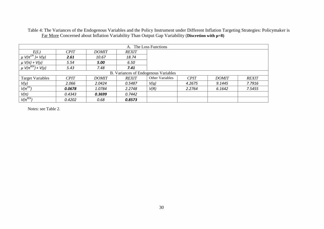
Table 4: The Variances of the Endogenous Variables and the Policy Instrument under Different Inflation Targeting Strategies: Policymaker is
Far More Concerned about Inflation Variability Than Output Gap Variability (Discretion with µ=8)
Notes: see Table 2.
A. The Loss Functions
E(L) CPIT DOMIT REXIT μ V(πCPI )+ V(y) 2.61 10.67 18.74
μ V(π) + V(y) 5.54 5.00 6.50
μ V(πREX) + V(y) 5.43 7.48 7.41 B. Variances of Endogenous Variables
Target Variables CPIT DOMIT REXIT Other Variables CPIT DOMIT REXIT
V(y) 2.066 2.0424 0.5487 V(q) 4.2675 9.1445 7.7916
V(πCPI) 0.0678 1.0784 2.2748 V(R) 2.2764 6.1642 7.5455
V(π) 0.4343 0.3699 0.7442
V(πREX) 0.4202 0.68 0.8573

31
Table 5: The Variances of the Endogenous Variables and the Policy Instrument under Different Inflation Targeting Strategies: Demand-Side
Variances are Four Times as Large as the Variance of Cost-Push Shock (Discretion, μ=1, =4, and
).
Notes: The off-diagonal scores in part A of the table have been omitted as they do not provide additional useful information not already contained in Table 2.
See also Table 2.
A. The Loss Functions
E(L) CPIT DOMIT REXIT μ V(πCPI )+ V(y) 3.42 NA NA
μ V(π) + V(y) NA 1.32 NA
μ V(πREX) + V(y) NA NA 0.99 B. Variances of Endogenous Variables
Target Variables CPIT DOMIT REXIT Other Variables CPIT DOMIT REXIT
V(y) 1.8893 0.1291 0.0098 V(q) 6.8465 19.334 22.766
V(πCPI) 1.5350 6.3300 8.1116 V(R) 6.5663 15.467 20.018
V(π) 0.7834 1.1915 1.3972
V(πREX) 0.8123 0.9441 0.9803

32
Table 6: The Variances of the Endogenous Variables and the Policy Instrument under Different Inflation Targeting Strategies: Policymaker is
Far More Concerned about Inflation Variability than Output Gap Variability and Variances of Demand-Side Shocks are Fourfold the
Variance of Cost-Push Shock (Discretion, μ=8, =4, and
).
Notes: see Tables 2 and 5.
A. The Loss Functions
E(L) CPIT DOMIT REXIT μ V(πCPI )+ V(y) 5.97 NA NA
μ V(π) + V(y) NA 6.34 NA
μ V(πREX) + V(y) NA NA 7.41 B. Variances of Endogenous Variables
Target Variables CPIT DOMIT REXIT Other Variables CPIT DOMIT REXIT
V(y) 5.1601 2.8186 0.5487 V(q) 5.1372 16.0047 24.8377
V(πCPI) 0.1015 2.5808 7.7295 V(R) 7.7441 11.3731 22.5243
V(π) 0.4379 0.4407 1.0851
V(πREX) 0.4559 0.6833 0.8573
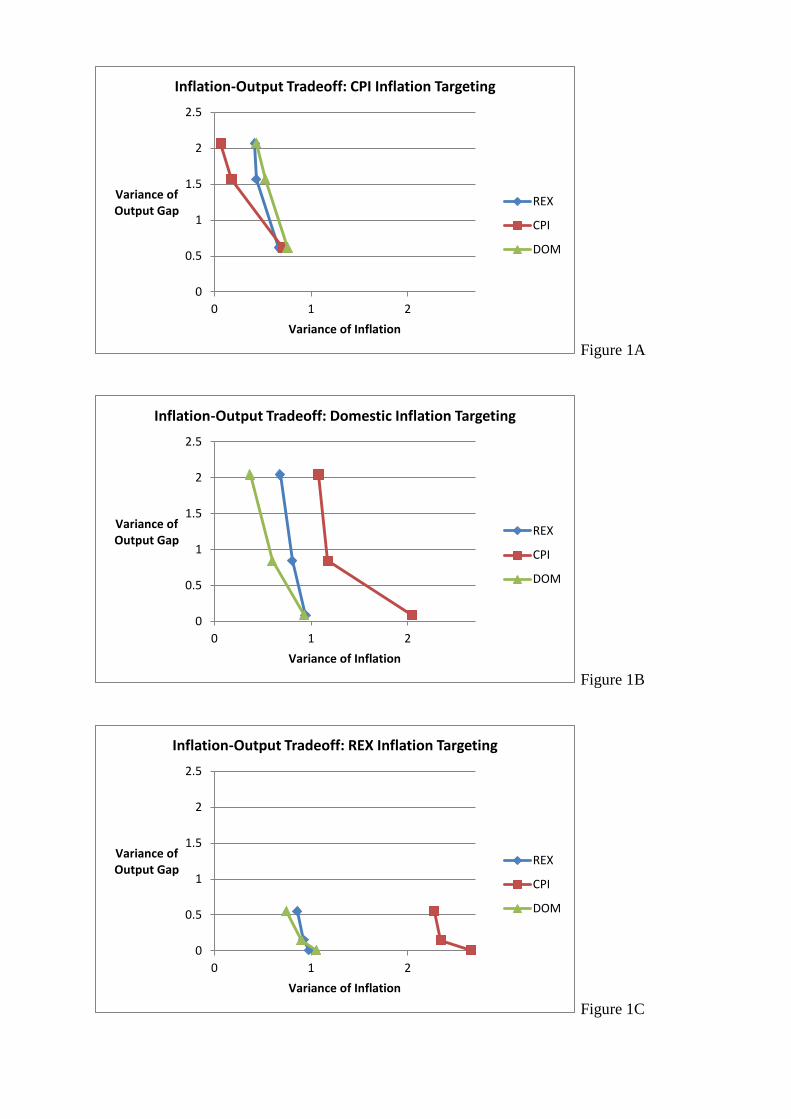
Figure 1A
Figure 1B
Figure 1C
0
0.5
1
1.5
2
2.5
0 1 2
Variance of Output Gap
Variance of Inflation
Inflation-Output Tradeoff: CPI Inflation Targeting
REX
CPI
DOM
0
0.5
1
1.5
2
2.5
0 1 2
Variance of Output Gap
Variance of Inflation
Inflation-Output Tradeoff: Domestic Inflation Targeting
REX
CPI
DOM
0
0.5
1
1.5
2
2.5
0 1 2
Variance of Output Gap
Variance of Inflation
Inflation-Output Tradeoff: REX Inflation Targeting
REX
CPI
DOM

34
Figure 1D
0
1
2
3
4
5
6
7
8
9
0 2 4 6 8
Variance of Interest Rate
Variance of Real Exchange Rate
Variances of RealExchange and Interest Rate
REX
CPI
DOM
45 ° Line