This paper presents preliminary findings and is being distributed to economists

and other interested readers solely to stimulate discussion and elicit comments.

The views expressed in this paper are those of the authors and do not necessarily

reflect the position of the Federal Reserve Bank of New York or the Federal

Reserve System. Any errors or omissions are the responsibility of the authors.

Federal Reserve Bank of New York

Staff Reports

What Predicts U.S. Recessions?

Weiling Liu

Emanuel Moench

Staff Report No. 691

September 2014

What Predicts U.S. Recessions? Weiling Liu and Emanuel Moench

Federal Reserve Bank of New York Staff Reports, no. 691

September 2014

JEL classification: C52, C53, E32, E37

Abstract

We reassess the predictability of U.S. recessions at horizons from three months to

two years ahead for a large number of previously proposed leading-indicator variables.

We employ an efficient probit estimator for partially missing data and assess relative

model performance based on the receiver operating characteristic (ROC) curve. While

the Treasury term spread has the highest predictive power at horizons four to six

quarters ahead, adding lagged observations of the term spread significantly improves the

predictability of recessions at shorter horizons. Moreover, balances in broker-dealer

margin accounts significantly improve the precision of recession predictions, especially

at horizons further out than one year.

Key words: recession predictability, ROC, term spread, leading indicators, efficient probit

estimator

_________________

Liu: Harvard Business School (e-mail: wliu@hbs.edu). Moench: Federal Reserve Bank of New

York (e-mail: Emanuel.moench@ny.frb.org). The views expressed in this paper are those of the

authors and do not necessarily reflect the position of the Federal Reserve Bank of New York or

the Federal Reserve System.

1 Introduction

Accurately predicting business cycle turning points, and in particular impending economic

recessions, is of great importance to households, businesses, investors and policy makers alike.

Prior research has documented that a variety of economic and financial variables contain pre-

dictive information about future recessions in the United States. Most prominently, Estrella

and Hardouvelis (1991) and Estrella and Mishkin (1998) have documented that the slope of

the term structure of Treasury yields has strong predictive power for US output growth and

US recessions at horizons up to eight quarters into the future. Other variables that have

been considered as leading recession indicators include stock prices (Estrella and Mishkin

(1998)), the index of Leading Economic Indicators (Stock and Watson (1989), Berge and

Jorda (2011)), credit market activity (Levanon, Manini, Ozyildirim, Schaitkin, and Tanchua

(2011)), as well as various employment and interest rate measures (Ng (2014)).

In this paper, we reassess the predictability of US recessions since 1959 using a wide variety

of leading indicator variables that have been considered in the academic and practitioner

literature. Consistent with most of the prior literature, we use the business cycle dating

chronology provided by the National Bureau of Economic Research (NBER) as the bench-

mark series of business cycle turning points. While the NBER recession indicator is a binary

variable, most leading indicators have continuous distributions. Thus, much of the empirical

literature has used the nonlinear probit model to map changes in predictor variables into

recession forecasts, and we follow this tradition.

The probability of a recession implied by the probit model is rarely exactly zero or one. Thus,

a cutoff is usually adopted such that a predicted probability above the cutoff is classified

as a recession. In order to objectively evaluate the model’s ability to categorize future time

periods into recessions versus expansions over an entire spectrum of different cutoffs, one

needs to complement the probit model with a classification scheme. A classification scheme

that has long been used in the statistics literature but has only recently found its way into

economic research is the receiver operating characteristic (ROC) curve (see, for example,

1

Khandani, Kim, and Lo (2010), Jorda and Taylor (2011), Jorda and Taylor (2012)). The

ROC curve is computed in several steps. First, for a given grid of cutoff values of the im-

plied recession probability, one calculates the percentage of true positives and false positives

for classifying all periods in the sample. One then plots the percentage of true and false

positives against one another for the entire grid to create the receiver operating curve. One

method of comparing the predictive ability of classifiers across a spectrum of cutoff values is

to integrate the area under the ROC curve, creating the AUROC. A model which delivers a

perfect classification of all time periods into recession and expansion would only have true

positives and no false positives and an AUROC equal to one. In contrast, a model which is

the equivalent of a random guess would have on average an equal number of true and false

positives, which corresponds to an AUROC equal to 0.5. Hanley and McNeil (1983) derive

a t-test for the hypothesis that the predictive ability of two different classifiers are equal

by using their AUROC’s. We use their test in order to discriminate between the predictive

ability of different recession indicators considered in the literature.

Our main findings can be summarized as follows. The Treasury term spread predicts best

at horizons of one year and more. That said, some indicators add to the predictive ability of

the term spread at these horizons. In particular, margin debit at NYSE brokers and deal-

ers, a measure of leverage in the financial sector, significantly improves the in-sample and

out-of-sample predictive power of the probit model when considered jointly with the term

spread at these longer horizons. This highlights the importance of financial intermediary

balance sheet conditions in the transmission of economic shocks (see, for example, Adrian

and Shin (2010) and Adrian, Moench, and Shin (2010)). While the importance of financial

intermediary leverage for the pricing of risk has been empirically documented by Adrian,

Etula, and Muir (2012) and Adrian, Moench, and Shin (2013), to the best of our knowledge,

its usefulness for the predictability of recessions has not previously been studied.

At horizons shorter than one year ahead, we find that adding six-month lagged observations

of the Treasury term spread significantly improves the predictive power of the probit model

2

to predict recessions. This suggests that at these shorter horizons there is predictive infor-

mation not only in the contemporaneous steepness of the Treasury yield curve, but also in

the lagged term structure slope. The negative sign on the coefficient of lagged spread has

two implications: persistence and change. First, if spreads were negative six-months ago,

then there is a higher probability of recession in the future. Second, given the same starting

value of spread six-months ago, a sharper drop in the spread since then leads to a higher

probability of recession in the future. In addition to the contemporaneous and lagged Trea-

sury term spreads, a number of other variables also contain predictive information about

future recessions at horizons less than one year ahead. In particular, the annual return on

the S&P500 stock market index, the Michigan survey of consumer expectations, and again

the margin debit at NYSE brokers and dealers significantly increase the predictive power of

the probit model when added to the Treasury term spread.

Our paper is related to a large literature on predicting real output growth and recessions

using financial and macroeconomic leading indicators. Estrella and Hardouvelis (1991) first

popularized the Treasury term spread as a predictor of future output growth and recessions.

They found that it has greater predictive power than the Leading Indicator Index and outper-

forms survey forecasts both in- and out-of-sample. Estrella and Mishkin (1996) and Estrella

and Mishkin (1998) considered the out-of-sample performance of a range of macroeconomic

and financial variables both one-at-a-time and in combination. Their findings suggest that

in the short run, stock returns are a valuable leading indicator. However, at horizons of one

year ahead or more, the Treasury term spread is still the single best performing predictor.

Dueker (1997) revisited the term spread as a leading indicator within the context of the

probit model studied in our paper. Confirming earlier results, he found the term spread to

be the single best recession predictor when compared to other leading economic indicators

and financial variables, and showed that this finding is robust to augmentation of the probit

model with lagged dependent variables and Markov switching. Chauvet and Potter (2005)

examine further extensions of the yield curve probit model, including a business cycle de-

3

pendent model, a model with autocorrelated errors, and combinations of these extensions.

They conclude that the more sophisticated models capture the predictive instability of the

yield curve better by allowing for breakpoints.

While all of the above cited papers have studied the predictive power of the term spread for

output growth and recessions in the U.S., some authors have documented similarly strong

predictive power of government bond yield spreads in other countries. For example, Duarte,

Venetis, and Paya (2005) find that yield spreads predict recessions in the European Mon-

etary Union. Moreover, examining both the U.S. and Germany, Nyberg (2010) concludes

that the domestic term spread remains the best recession predictor.

Recently, Rudebusch and Williams (2009) have found that the term spread consistently

outperforms even professional forecastors in predicting recessions. This is surprising as

these forecasters have a wealth of information and many other indicators available to them.

Croushore and Marsten (2014) confirm that Rudebusch and Williams’ findings are robust

across several dimensions including the sample choice, the use of rolling regression windows,

and various measures of real output. Moreover, Lahiri, Monokroussos, and Zhao (2013)

report that the result remains valid even after further augmenting the model with factors

extracted from a large macroeconomic dataset. These papers’ findings highlight the singular

importance of the Treasury term spread as a predictor of recessions and justify our use of

this indicator as the benchmark predictor variable.

Methodologically, our paper borrows from Berge and Jorda (2011), who use the AUROC

to both validate the NBER’s business cycle chronology as well as investigate which leading

indices work best as a classification mechanism for recessions. They find no support for sta-

tistically significant improvements of the parametric models over the NBER dates. Hence,

their results also support our use of the NBER business cycle chronology as reference for the

recession classification ability of the various probit models that we consider.

Our paper is organized as follows. Section 2 discusses the empirical methodology used to

predict recession probabilities and evaluate the classification of future recession and expan-

4

sion periods. Section 3 provides a description of the various recession indicators used in our

analysis. Section 4 summarizes the in-sample and out-of-sample recession prediction results.

Finally, Section 5 provides a discussion of the empirical findings.

2 Methodology

In this section, we briefly describe the empirical methods used in the paper. We start by

revisiting the standard probit model which we use to estimate the recession probabilities

as functions of observable predictor variables. We then briefly discuss an extension which

allows for the inclusion of partially unobserved predictor variables. Finally, we describe

the AUROC measure and related statistical tests which we employ to discriminate between

models.

2.1 Predicting Recessions

The state of the business cycle is a binary variable, taking on the value of one during a

recession and zero during an expansion. On the other hand, most leading indicators are

continuous variables. In order to account for this, a common tool to predict recessions is the

probit model (see Estrella and Hardouvelis (1991), Estrella and Mishkin (1996), Estrella and

Trubin (2006),Wright (2006)) which allows a mapping from a set of continuous explanatory

variables into a binary dependent variable. While other methods are available for predicting

binary response variables, we restrict ourselves to this popular class of models for its sim-

plicity and ease of use.

The model is characterized by the simple equation

P (RECt+k = 1) = Φ (α0 + α′1Xt) , (1)

5

where REC is a binary variable which takes on values of one in recessions and zero in

expansions, Xt is a n × 1 vector of predictor variables observed in period t, and Φ denotes

the cumulative density function of the standard normal distribution. Letting α = (α0, α′1)′ ,

the probit model maximizes the log likelihood function

ln ` (α) =T∑t=1

[RECt+k ln Φ (α0 + α′1Xt) + (1−RECt+k) ln (1− Φ (α0 + α′1Xt))] (2)

Hence, given time series observations for the predictor variables X and the response

variable REC, one can numerically solve for the maximum likelihood estimates α.

Some of the predictor variables we will consider in our empirical analysis are not observed

over the full sample period. We therefore need to adjust the probit model to allow for missing

observations. One commonly used method of handling missing data is to disregard the dates

on which any variables are missing, but this method inefficiently discards potentially useful

data. Instead, we employ the efficient “probitmiss” estimator, recently proposed by Conniffe

and O’Neill (2011), which allows us to incorporate all relevant data.

Building off of Chesher (1984), Conniffe and O’Neill’s model assumes that there exists one

underlying unobservable, continuous latent variable Yi and an observed binary variable Zi

which follows the relationship:

Zi = 1 if Yi > 0

Zi = 0 if Yi < 0.

The regressors are grouped into two categories, denoted in vector form: Xi (complete) and

Wi (incomplete). There are k number of X’s, and l number of W ’s. We observe the complete

sample of observations {Xi,Wi, Zi} for i =1,2,. . . r. This leaves (n−r) observations on which

{Xi, Zi} alone are measured. They follow the relationship:

Yi = X′

iBx +W′

iBw + εi. (3)

6

To make use of the n− r non-missing observations, assume:

W′

i = X′

iC + u′

i, (4)

where C is a (k x l) matrix of parameters and ui ∼MVN(0,Σ). Then, combining (3) and

(4), one obtains:

Yi = X′

i(Bx + CBw) + eyi , (5)

where, conditional on Xi, (eyi ,Wi) are multivariate normally distributed. The assumption

of conditional joint normality is analytically convenient and allows for efficient estimation.

Conniffe and O’Neill (2011) show that their proposed estimator is robust to various depar-

tures from the parametric assumptions in (4).

Rather than explicitly restating the estimator and its asymptotic variance derived by Con-

niffe and O’Neill (2011), we simply summarize the various estimation steps:1

1. Run an OLS regression of X on W for the sample with r complete observations.

2. Run a standard probit of Y on X and W for the sample with r complete observations.

3. Run a probit of Y on X for just the sample with n− r missing observations

4. Calculate the coefficients and standard errors for the probitmiss estimator using as

inputs the estimation outputs from steps(1)-(3).

It is important to point out that in addition to the assumption of conditional multinor-

mality, the efficient probit estimator requires that the missing data for W are missing at

random (MAR). In other words, the reason for the data’s absence should not be related to

an omitted variable that is correlated with recessions, such as the state of the business cycle.

Since our missing data are only missing at the beginning of the dataset due to limitations

of our database, the MAR assumption is naturally satisfied.

1For further details, we refer the interested reader to the paper by Conniffe and O’Neill (2011).

7

2.2 Model Selection

Previous research has used various different metrics to evaluate the fit of recession prediction

models. For example, Moore and Shiskin (1967) present an explicit scoring system for busi-

ness cycle indicators, focusing on the length of lead before business cycles turns, smoothness

of the series, clarity of cyclical movements, and relationship to general business activity,

among other criterion. Estrella and Mishkin (1996) and Estrella and Mishkin (1998) use

the pseudo R-squared to evaluate the fits of probit models. Finally, Wright (2006) employs

the BIC criterion to measure the fit of his model in-sample and root mean squared forecast

errors to evaluate the fit of his out-of-sample forecasts.

However, all of these evaluation measures focus on model fit and not specifically classifi-

cation ability, which is the object of interest in our application. Berge and Jorda (2011)

have recently used the Receiver Operating Characteristic (ROC) curve to assess the reces-

sion classification ability of various leading indicators. The ROC curve is a useful measure,

because it precisely captures the ability of each model to accurately categorize recessions

and expansions. In particular, by using the area under the ROC curve (AUROC), one can

evaluate the categorization ability of the model over an entire spectrum of different cut-

offs for determining a recession, instead of evaluating predictive power at any one arbitrary

threshold.

In a seminal paper, Peterson and Birdsall (1953) first developed the basic ROC method-

ology. The procedure has been widely used in statistics and other fields, but it has only

recently found its way into the economics literature (see, for example, Khandani, Kim, and

Lo (2010), Jorda and Taylor (2011), and Jorda and Taylor (2012)). Applied to the context

of predicting recessions, it can be summarized as follows:

1. Let

Xt =

1, if in recession

0, otherwise(6)

denote the true, observed state of the economy. Let Pt be the prediction of Xt, or the

8

probability of recession, given by the probit model, where 0 ≤ Pt ≤ 1.

2. Define evenly spaced thresholds (denoted C∗) along the interval [0,1]. A larger num-

ber of thresholds leads to a smoother ROC curve with more points. For example, a

potential set with 50 thresholds would be: C∗i ={0,0.05,. . . 0.95,1}.

3. For each given threshold, C∗i , record the model’s predicted categories. More specifi-

cally, define the predicted categorization of Xt,or Xt, in the following way:

Xt =

1, if Pt ≥ C∗i

0, if Pt < C∗i

(7)

4. Comparing the true Xt to predicted categorizations Xt, calculate the percentage of

true positives (PTP) and percentage of false positives (PFP). More specifically, they

can be defined using the sum of two indicator variables:

PTP =1

nR

N∑t=1

I tpt ; where I tpt =

1, if Xt = 1 and Xt = 1

0, otherwise(8)

PFP =1

nE

N∑t=1

Ifpt ; where Ifpt =

1, if Xt = 0 and Xt = 1

0, otherwise(9)

and where nR is the number of times the true Xt was in a recession and nE is the

number of times the true Xt was not in a recession, such that nR+nE=N , where N is

the total number of observations in our sample.

5. For each C∗i , create a set of coordinates: (PFPi,PTPi).

9

6. After a coordinate is created for each threshold, plot the coordinates across all thresh-

olds where the false positive rate is on the x-axis and the true positive rate is on the

y-axis. Connect these coordinates to trace out the ROC curve.

In summary, the ROC curve pinpoints the percent of false negatives one would have to

trade for one additional percent of true positives. A model with 100% accuracy would draw

a ROC curve hugging the top left corner. A model which is the equivalent of a random

guess would follow a 45% diagonal that runs from the bottom-left corner to the top-right

corner. By construction, if we defined Xt in terms of expansions (i.e. let Xt equal one during

expansions and zero otherwise) instead of recessions, the new curve would look symmetric

to the old curve about a 45 degree line from the bottom-right corner to the top-left corner.

The area under the curve, by geometry, would then remain exactly the same as before.

Due to its ease of application and intuitive visual interpretation, the area under the ROC

curve (AUROC) is a popular measure of classification ability for a given model. In our

empirical analysis in Section 4, we will therefore compare the recession classification ability

of various different probit models using their implied AUROC’s. As discussed in Berge and

Jorda (2011), a simple nonparametric estimate of the AUROC is given by

AUROC =1

nRnE

nE∑i=1

nR∑j=1

{I(Zi > Xj) +

1

2I(Zi = Xj)

}, (10)

where I(·) is the indicator function, X are the observations classified to be a recessionary

period and Z are the observations classified to be an expansionary period. nR and nE are

the true numbers of recessionary and expansionary periods, respectively.

We can assess the statistical significance of a model-implied AUROC using the asymptotic

standard error derived by Hanley and McNeil (1982). The variance is given by:

σ2 =1

nRnE

[AUROC(1−AUROC)+(nR−1)(Q1−AUROC2) + (nE−1)(Q2−AUROC2)

]1/2,

10

where Q1 = AUROC(2−AUROC)

, and Q2 = 2AUROC2

(1+AUROC), see again Hanley and McNeil (1982).

Hanley and McNeil (1983) extend this estimator further by developing a t-statistic for com-

paring AUROCs across multiple models, taking into account the correlation between the two

areas being compared. The t-statistic is given by:

t =AUROC1 − AUROC2√

σ21 + σ2

2 − 2rσ1σ2. (11)

Here, AUROC1 and AUROC2 are the areas under the curve for models 1 and 2 which are

being compared. Similarly, σ21 and σ2

2 refer to the variances of the AUROCs for model 1 and

model 2, respectively. Finally, r is the correlation between the two AUROCs. To obtain r,

one needs to compute two intermediate parameters rE and rR, which are the correlations

for the expansionary observations and recessionary observations, respectively, across the

two models. These correlations can be calculated using either Pearson product-moment

correlation or the Kendall tau rank correlation coefficient. In our paper, we choose to use

the latter. See Hanley and McNeil (1983) and Jorda and Taylor (2011) for more details on

the test statistic and its implementation.

3 Data

We use monthly U.S. data for the sample period January 1959 to December 2011. The

dependent variable is a binary recession indicator which takes on the value of one during a

recession and zero during an expansion, both as defined by the NBER business cycle dating

committee. The committee meets periodically to judge whether a peak or trough in eco-

nomic activity has occurred, taking into account a variety of economic activity indicators,

including real GDP measured on the product and income sides, economy-wide employment,

real income, as well as indicators covering real parts of the economy, such as retail sales and

industrial production.2 The NBER’s dating rules are widely regarded as the benchmark for

2See http://www.nber.org/cycles/recessions.html.

11

US business cycles. Moreover, as discussed in the introduction, Berge and Jorda (2011) find

no improvement of a number of sophisticated parametric models over the recession classifi-

cation ability of the NBER.

For in-sample recession prediction, our sample runs from 1959 to 2011 and covers a total of

seven recessions, which range in duration from six to 18 months. We also conduct out-of-

sample forecasts, using the period of January 1959 to August 1985 (which covers a total of

four recessions) as our training sample, and the period from September 1985 through Decem-

ber 2011 (covering three recessions) as our forecasting sample. Our explanatory variables are

taken from Haver Analytics, with the exception of real-time macroeconmic indicators, which

come from the ArchivaL Federal Reserve Economic Database (ALFRED). Following Estrella

and Hardouvelis (1991), Estrella and Mishkin (1998), and others, we use the term spread,

precisely defined as the difference between the ten-year and the three-month Treasury yield

(“10y- 3m spd ”), as our benchmark predictor variable. We then assess whether additional

lags of the term spread as well as other candidate predictor variables add predictive power

to the benchmark model.

Based on prior research, we consider the following list of additional predictor variables. First,

following Estrella and Mishkin (1998), we add several financial indicators including returns on

the S&P500 common stock price index (“S&P 500, 1y% change”, “S&P 500, 3y % change”)

and the interest rates of the 3-month (“3m rate”) and 10-year Treasuries (“10y rate”). Sec-

ond, we include each component of the Conference Board’s Leading Economic Index (LEI)

(see Levanon, Manini, Ozyildirim, Schaitkin, and Tanchua (2011)). These indicators have

been selected for their ability to signal peaks and troughs in the business cycle, and the

aggregate index has been shown to drop ahead of recessions and rise before expansions.

The individual factors consist of: average weekly hours of manufacturing (“Avg wkly hrs

(manufacturing)”); average weekly initial claims for unemployment insurance (“Avg initial

claims”); manufacturer’s new orders, goods, and materials (“New orders, goods, materials”);

the ISM index of new orders (“ISM new orders index”); manufacturers’ new orders, nonde-

12

fense capital goods excluding aircraft (“New orders, non-defense”); building permits, new

private housing units (“Building permits”); the rate of the 10-year Treasury note less federal

funds (“10yr-FF spread”); average consumer expectations (“Michigan consumer survey”);

and the Leading Credit Index.

The latter was introduced by the Conference Board to supplement the Leading Economic

Index and reflect potential structural changes in the changing credit and financial markets.

Its components were selected in the spirit of financial intermediation models as laid out

by Adrian and Shin (2010) and are tested for their ability to signal business cycle changes

using a Markov Switching model (see Levanon, Manini, Ozyildirim, Schaitkin, and Tanchua

(2011)). We include each of the LCI’s components offered at a monthly frequency or greater

going back to at least 1985: the LIBOR 3-month less 3-month Treasury bill yield spread

(“LIBOR 3 month”), balances in Broker-Dealer margin accounts (“Debit margins (BD)”),

and the AAII Sentiment Survey’s Market Survey of the spread between bearish and bullish

sentiments (“Bear less bull”).

Finally, we add a number of predictor variables following the recent findings of Ng (2014).

In her paper, Ng examines a comprehensive list of 132 different real and financial indica-

tors and assesses their relevance for predicting recessions. We include all of the 14 unique

variables found to be most important using cross-validation boosting techniques as well as

the 4 additional unique variables found through a rolling window exercise. This list includes

the spreads between the yields of several constant maturity Treasuries with the fed funds

(FF) rate (“3m/6m/1yr/2yr/5yr/30yr- FF spread”); employment hours for total non-farm,

government, manufacturing, and mining (“Emp: total/govt/mfg/mining”); NAMP index of

consumer commodity prices (“NAPM com price”); NAPM vendor deliveries (“NAPM ven-

dor del”); NAPM inventories index (“NAPM invent”); and the US$-Yen exchange rate (“Ex

rate: Japan”).

Table 1 provides a list of all the predictor variables that we consider, their available time

span, the database from which they originate, and the transformations that we used to ren-

13

der the series stationary. These transformations directly follow those used in the papers

cited above. Since macroeconomic variables are often revised after their release dates and

these revisions are not available to the economist for out-of-sample forecasting, we use real-

time, or the first-release, indicators whenever possible. When available, the real-time data is

collected from the ALFRED database. For several macroeconomic variables, real-time data

do not exist before 1985. These variables are marked with an asterisk in Table 1 and are

excluded from our out-of-sample analysis.

4 Results

In this section, we describe our results from comparing various probit model specifications at

different horizons. We divide our analysis into in-sample versus out-of-sample forecasts. In-

sample forecasts are estimated over the entire sample from January 1959 to December 2011.

Out-of-sample forecasts are estimated using the first half of the sample, from January 1959

to August 1985, and then evaluated using the second half of the sample, from September

1985 to December 2011. In both exercises, we consider forecasts at the 3-, 6-, 12-, 18-, and

24-months ahead horizons. At each horizon, we begin by estimating a baseline probit model

using just the term spread as explanatory variable (Estrella and Hardouvelis (1991)). Then,

we augment the benchmark model with the six-month lagged term spread as an additional

explanatory variable. We do so in order to assess whether it is the contemporaneous level or

the change in the spread that is important for predicting recessions. Moreover, this allows us

to test whether the added leading indicators contain predictive information over and above

that captured in the term spread.

Finally, one at a time, we add each of the variables shown in Table 1 to the spread and

lagged spread models. We use the AUROC to evaluate the performance of each model and

also to compare their forecasting abilities to the two baseline models using the t-statistic

presented in Section 2.

14

4.1 In-sample Analysis

The results of our in-sample probit regressions are summarized in Table 2. The table is bro-

ken down into panels A through E, corresponding to 3-, 6-, 12-, 18-, and 24-months ahead

forecast horizons, respectively. Each panel reports results from the spread-only model, a

spread and six-month lagged spread model, and three additional models. These three addi-

tional models use the term spread, the lagged term spread, and one of three best-performing

additional indicators as determined by the AUROC metric. For each model, we report its

AUROC as well as its t-statistic when compared to the two baseline models: spread-only

and spread augmented with six-month lagged spread.

Figures 1 - 3 summarize the findings in Table 2 visually. In these figures, the plots are paired

by forecast horizon. The top graph shows the predicted probability of recession over time,

with actual recessions shown as shaded grey areas. The second graph shows the correspond-

ing ROC curves calculated as described in Section 2. In each graph, the three lines shown

represent the estimates from the spread-only model (blue line), the spread and lagged spread

model (green line), and one additional model with best performance as determined by the

AUROC (red line).

At the three-months ahead horizon, we find that we can significantly improve the spread-only

model by simply adding a six-month lag of the term spread. In fact, doing so increases the

AUROC from 0.67, which is only slightly better than a random guess, to 0.85, which is quite

accurate. The two AUROC’s are significantly different at the 1% level, with a t-statistic of

5.5. Furthermore, we can improve the spread and lagged-spread model by including one of

many additional indicators. The best one is the annual return on the S&P 500 index, which

has a near-perfect AUROC of 0.95 and a t-statistic of 4.1 when compared to the spread and

lagged spread model. The other two best-performing additional indicators are the Michigan

consumer confidence survey and debit balances at margin accounts at broker dealers, which

have AUROC’s of 0.929 and 0.927 respectively.

At the six-months ahead horizon, we again see that adding a six-month lagged spread signif-

15

icantly improves the recession classification ability of the probit model, raising the AUROC

from 0.78 to 0.87. In addition, the Michigan consumer survey continues to be one of the top

additional indicators. The other two are the 5-year Treasury yield - fed funds rate spread

and building permits. Again, we find that one can significantly improve upon a model with

spread and lagged spread by adding any of these three additional indicators. Hence, there is

predictive information in these other variables beyond that captured by the Treasury term

spread.

At the twelve-months ahead horizon, the spread-only model performs remarkably better than

at the shorter horizons with an AUROC of 0.87. While adding the lagged spread improves

the predictive ability somewhat, it does not do so significantly. Similar to the six-months

horizon, we find that the model with the 5-year Treasury-FF spread performs the best, im-

proving upon the spread-only model with an AUROC of 0.90 and a only a t-statistic of 2.08.

The two next best models use the 1-year Treasury-FF spread and the NAPM commodity

price index, respectively.

Turning to the 18-months ahead forecast horizon, we see that the predictive ability of the

spread-only model with an AUROC of 0.81 is slightly worse than at the twelve-months ahead

horizon but better than the three- and six-months ahead horizons. Given these results we

find that, not surprisingly, adding a six-month lagged spread actually marginally hurts the

predictive ability of the model instead of improving it. Similar to the twelve-months ahead

horizon, the NAPM commodity price index is among the top three additional predictor

variables. It is outperformed only by the model using margin debit at broker-dealers as

an additional predictor. In fact, broker dealer margin debit is the only predictor variable

that significantly increases the AUROC when added to the two baseline models. This is

intriguing given that the previous literature is generally in consensus that at the twelve- and

eighteen-months ahead horizon, the spread-only model performs the best.

Finally, at the 24-months ahead horizon, we see that predictive ability is generally much

lower for all models although still quite a bit better than a simple random guess model. The

16

spread-only model has an AUROC of 0.69, which makes it comparable to its counterpart at

the three-months ahead horizon (0.67). Adding the lagged spread improves the prediction

ability but only marginally so. On the other hand, we also find that the addition of mar-

gin debit at broker-dealers, new non-defense orders, or the NAPM commodity price index

significantly improves the two baseline models. All three perform about equally well with

AUROC’s ranging from 0.79 to 0.77. While these are not strong predictive abilities, they are

higher than similar models estimated just using components of the LEI, which are considered

the benchmark leading indicators (see Berge and Jorda (2011)).

Importantly, the probitmiss estimator by Conniffe and O’Neill (2011) allows us to find strong

and significant forecasting value in variables which have missing observations and which may

have been excluded from our analysis otherwise. More specifically, the broker-dealer margin

debit variable and the Michigan survey of consumer expectations both start later than Jan-

uary 1959 which marks the beginning of our sample, yet we find that they are often useful

in improving the in-sample recession forecasting ability.

4.2 Out-of-sample Analysis

The results of our baseline and best performing out-of-sample probit regressions are sum-

marized in Table 3. As before, the table is organized in five panels corresponding to the

five different forecast horizons. Each panel shows the AUROC for the spread-only model,

the spread and lagged-spread model, and the three best models obtained by adding a third

predictor variable to the spread and lagged spread baseline model. For each model, we report

its AUROC as well as its t-statistic when compared to both baseline models.

Figures 1-3 summarize the findings in Table 3 visually. Again, the plots are grouped by pairs

depending on the forecast horizon, where the first graph shows the predicted probability of

recession over time and the second graph shows the corresponding ROC graphs calculated

by comparing the predicted probability with the NBER business cycle chronology. In each

of the latter graphs, the three lines represent the estimates from the spread-only model (blue

17

line), the spread and lagged spread model (green line), and the best performing model which

augments the spread and lagged spread model with an additional predictor variable (red

line).

At the three-months ahead horizon, we see that the spread-only model is little better than

a random guess, with an AUROC of only 0.56. This performance is notably worse than the

in-sample model, which has an AUROC of 0.67. One possible interpretation of this finding

is a shift in the predictive power of the term spread for recessions around the end of our

training sample in 1985. This is consistent with prior evidence for structural change in the

predictive relationship between the term spread and future output growth (see, for example,

Schrimpf and Wang (2010)). That said, adding a six-month lag of the term spread improves

the AUROC dramatically to 0.77 with an accompanying t-statistic of 4.34. In line with the

in-sample analysis, we find that the annual return on the S&P 500 index, the Michigan sur-

vey of consumer sentiment, and margin debit at broker-dealers are the three best performing

additional variables. They also significantly improve upon the spread and lagged spread

model. The best model, using the annual return on the S&P 500 index, has a near-perfect

predictive ability and an AUROC of 0.96.

Next, at the six-months ahead horizon, we find that the spread-only model performs worse

than its in-sample counterpart with an AUROC of 0.67. Again, adding the six-months lagged

spread significantly improves the model’s predictive ability, raising its AUROC to 0.79. Sim-

ilar to the three-months ahead horizon, we find that the annual return on the S&P 500 index

and margin debit at broker-dealers are useful leading indicators. Moreover, in line with the

in-sample analysis at this horizon, the remaining selected indicator is the 5-year Treasury

yield-fed funds rate spread. While the best additional indicator is the annual return on the

S&P 500 index, with a sizable AUROC of 0.90, all of the top three models with additional

indicators significantly outperform the spread and lagged spread model.

At the 12-months ahead horizon, the spread-only model has an AUROC of 0.86. This is

very similar to its in-sample counterpart, which has an AUROC of 0.87. Adding a six-month

18

lag of the term spread slightly increases the AUROC to 0.88 but the difference is not found

to be statistically significant. Consistent with the in-sample analysis, we find that the best

three additional indicators ranked by decreasing importance are the 5-year Treasury yield

- fed funds rate spread, the 1-year Treasury yield - fed funds rate spread, and the NAPM

commodity price index. These models’ AUROC’s are also very similar to their in-sample

counterparts, and, again, we find that we can significantly improve upon the spread-only

model by adding the 5- or 1-year Treasury yield - fed funds rate spreads.

At the 18-months ahead horizon, the spread-only model performs quite well with an AUROC

of 0.91, even better than at the 12-months ahead horizon. This is also remarkably better

than its in-sample counterpart, which only has an AUROC of 0.81. While other models

perform better than the spread-only model, we find their improvement to be statistically

insignificant at conventional levels. Unlike the shorter forecast horizons, we find that adding

the lagged spread actually decreases the AUROC to 0.88. However, adding margin debit

at broker-dealers, the ISM new orders index, or average initial claims slightly improves the

AUROC to 0.93, 0.91, and 0.90 respectively. That said, only the broker-dealer variable is

found to significantly improve the predictive power of the model with respect to the spread

and lagged spread model. However, when compared to the spread-only model the improve-

ment is statistically insignificant.

Finally, at the 24-months ahead horizon, we find that the spread-only model has an impres-

sive AUROC of 0.85. In fact, no other model performs better. Adding the lagged spread

decreases the AUROC to 0.81. The best model with an additional predictor is the NAPM

inventories index, which delivers an AUROC of 0.85. Comparing to the in-sample analysis,

we find that the out-of-sample forecasts perform even better than their in-sample counter-

parts at the 24-months ahead horizon. In fact, the best model in the in-sample analysis has

an AUROC of 0.79, which is lower than the corresponding out-of-sample estimation.

19

5 Summary of Findings and Concluding Remarks

In sum, our results imply the following main takeaways. First, consistent with the past

literature, we find that our ability to improve upon the spread-only model drops at longer

horizons of twelve months or greater. However, adding the 5-year Treasury - fed funds rate

spread significantly improves both the in- and out-of-sample forecasts at the twelve-months

ahead horizon. Moreover, our results indicate that adding the lagged term spread and mar-

gin debits at broker-dealers significantly improve both 18- and 24-months ahead in-sample

forecasts.

Second, there is valuable information not only in the contemporaneous Treasury term spread

but also in its dynamics. More specifically, one can drastically increase the recession predic-

tion ability for out-of-sample forecasts by adding lagged observations of the Treasury term

spread at short forecast horizons. In fact, adding six-months lagged observations of the Trea-

sury term spread essentially moves the model from one that is little better than a random

guess to a very accurate one. At longer horizons, the forecasting ability is generally worse

across model specifications. For instance, in the out-of-sample forecast analyses at horizons

longer than twelve months, the predictive ability decreases when the lagged spread is added

to the probit model.

Third, we find that margin debit at broker-dealers is a useful leading indicator. To the best

of our knowledge, this has not been appreciated in the previous academic literature. Models

which add the margin debit variable consistently rank among the top three models for the

three-, 18-, and 24-months ahead in-sample estimations, always significantly outperforming

the spread-only model. In addition, we find that models with this variable rank among the

top three for the thee-, six-, and 18-month ahead horizons for the out-of-sample estimations.

As margin debit at broker-dealers is typically considered to be a measure of leverage in

the financial system, its importance in predicting recessions highlights the role of financial

intermediary balance sheet management in the transmission of economic shocks.

20

Table 1: Summary of Key Variables This table reports all of the predictor variablesconsidered in our analysis. For each indicator, we report the series’ name, the transformationwe performed before using it in our analyses, the data source, and the time span for whichthe series is available. Transformation codes 1-6 correspond to levels, monthly log difference,annual log difference, annual difference, 6-months moving average smoother, and 12-monthsmoving average smoother, respectively. The data sources USECON, BCI, and ALFRED referto the U.S. Economics Statistics database in Haver Analytics, the Business Cycle Indicatorsdatabase in Haver Analytics, and the online ArchivaL Federal Reserve Economic Databaseat the St. Louis Fed, respectively. * denotes macroeconomic indicators for which we real-time data extending past 1985 are not available and which are thus excluded from ourout-of-sample analysis.

Series Name Code Source Time Span

10y- 3m spd 1 USECON Jan 1959-Dec 201110y rate 1 USECON Jan 1959-Dec 20113m rate 1 USECON Jan 1959-Dec 2011S&P 500, 1y % change 1 USECON Jan 1959-Dec 2011S&P 500, 3y % change 1 USECON Jan 1959-Dec 2011Leading credit index 1 BCI Jan 1959-Dec 2011Michigan consumer survey 1 BCI Jan 1978-Dec 2011Debit margins (BD) 1 BCI Jan 1960-Dec 2011Bear less bull 4 BCI Jul 1987-Dec 2011LIBOR 3 month 1 USECON Jan 1963-Dec 2011Baa-Aaa spread 1 USECON Jan 1959-Dec 2011Aaa-FF spread 1 USECON Jan 1959-Dec 2011Baa-FF spread 1 USECON Jan 1959-Dec 20113mo-FF spread 1 USECON Jan 1959-Dec 20116m-FF spread 1 USECON Jan 1959-Dec 20111yr-FF spread 1 USECON Jan 1959-Dec 20112yr-FF spread 1 USECON Jun 1976-Dec 20115yr-FF spread 1 USECON Jan 1959-Dec 201110yr-FF spread 1 USECON Jan 1959-Dec 201130yr-FF spread 1 USECON Mar 1977-Dec 2011Ex rate: Japan 2 USECON Jan 1959-Dec 2011Avg wkly hrs (manufacturing) 1 ALFRED Jan 1959-Dec 2011Avg initial claims * 3 BCI Jan 1959-Dec 2011New orders, goods, materials * 3 BCI Jan 1959-Dec 2011New orders, non-defense * 3 BCI Jan 1959-Dec 2011ISM new order index * 1 BCI Jan 1959-Dec 2011Building permits * 3 BCI Jan 1959-Dec 2011Emp: total 5 ALFRED Jan 1959-Sep 2010Emp: govt 5 ALFRED Jan 1959-Dec 2011Emp: mfg 6 ALFRED Jan 1959-Dec 2011Emp: mining 5 ALFRED Jan 1959-Dec 2011NAPM com price 1 ALFRED Jan 1959-Dec 2011NAPM vendor del * 1 USECON Jan 1959-Dec 2011NAPM invent * 1 USECON Jan 1959-Dec 201121

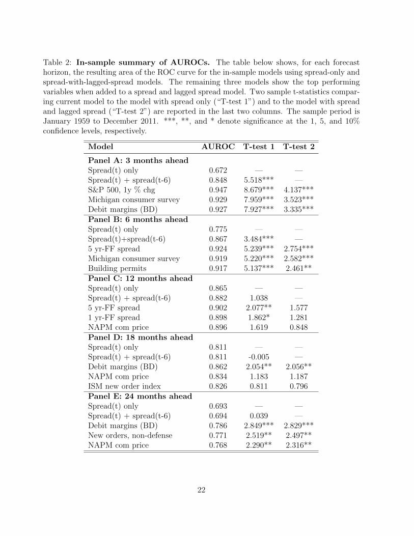
Table 2: In-sample summary of AUROCs. The table below shows, for each forecasthorizon, the resulting area of the ROC curve for the in-sample models using spread-only andspread-with-lagged-spread models. The remaining three models show the top performingvariables when added to a spread and lagged spread model. Two sample t-statistics compar-ing current model to the model with spread only (“T-test 1”) and to the model with spreadand lagged spread (“T-test 2”) are reported in the last two columns. The sample period isJanuary 1959 to December 2011. ***, **, and * denote significance at the 1, 5, and 10%confidence levels, respectively.

Model AUROC T-test 1 T-test 2

Panel A: 3 months aheadSpread(t) only 0.672 — —Spread(t) + spread(t-6) 0.848 5.518*** —S&P 500, 1y % chg 0.947 8.679*** 4.137***Michigan consumer survey 0.929 7.959*** 3.523***Debit margins (BD) 0.927 7.927*** 3.335***Panel B: 6 months aheadSpread(t) only 0.775 — —Spread(t)+spread(t-6) 0.867 3.484*** —5 yr-FF spread 0.924 5.239*** 2.754***Michigan consumer survey 0.919 5.220*** 2.582***Building permits 0.917 5.137*** 2.461**Panel C: 12 months aheadSpread(t) only 0.865 — —Spread(t) + spread(t-6) 0.882 1.038 —5 yr-FF spread 0.902 2.077** 1.5771 yr-FF spread 0.898 1.862* 1.281NAPM com price 0.896 1.619 0.848Panel D: 18 months aheadSpread(t) only 0.811 — —Spread(t) + spread(t-6) 0.811 -0.005 —Debit margins (BD) 0.862 2.054** 2.056**NAPM com price 0.834 1.183 1.187ISM new order index 0.826 0.811 0.796Panel E: 24 months aheadSpread(t) only 0.693 — —Spread(t) + spread(t-6) 0.694 0.039 —Debit margins (BD) 0.786 2.849*** 2.829***New orders, non-defense 0.771 2.519** 2.497**NAPM com price 0.768 2.290** 2.316**

22

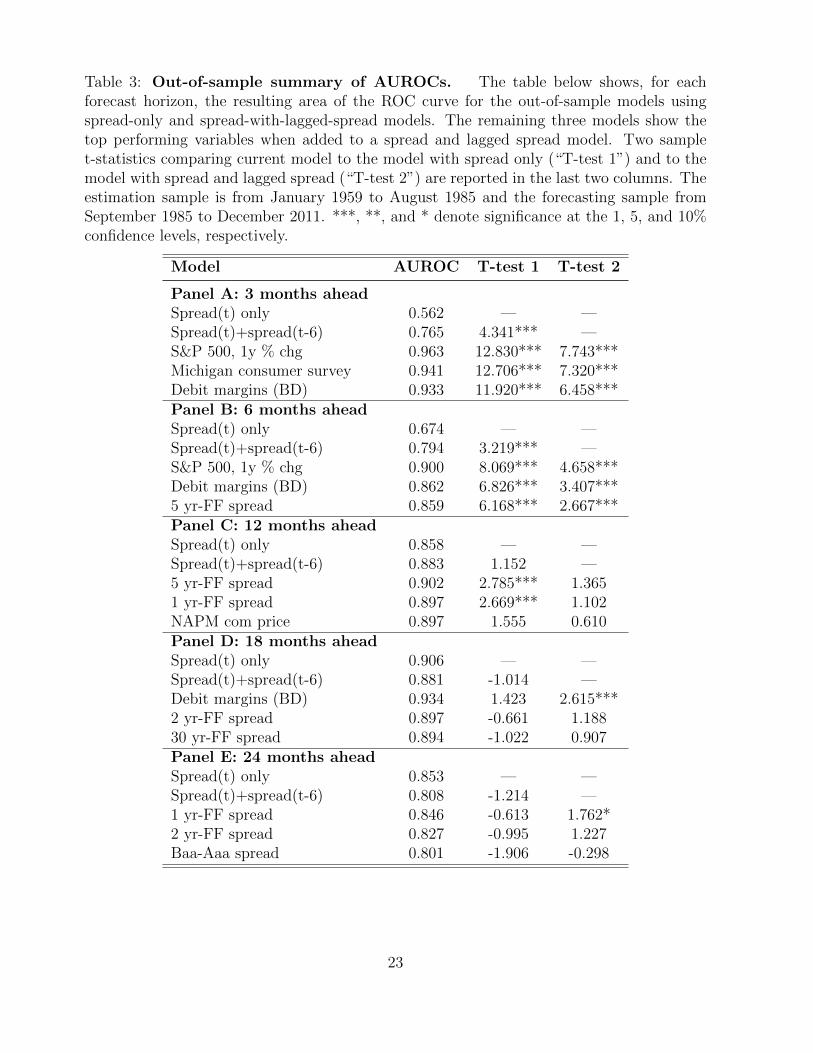
Table 3: Out-of-sample summary of AUROCs. The table below shows, for eachforecast horizon, the resulting area of the ROC curve for the out-of-sample models usingspread-only and spread-with-lagged-spread models. The remaining three models show thetop performing variables when added to a spread and lagged spread model. Two samplet-statistics comparing current model to the model with spread only (“T-test 1”) and to themodel with spread and lagged spread (“T-test 2”) are reported in the last two columns. Theestimation sample is from January 1959 to August 1985 and the forecasting sample fromSeptember 1985 to December 2011. ***, **, and * denote significance at the 1, 5, and 10%confidence levels, respectively.

Model AUROC T-test 1 T-test 2

Panel A: 3 months aheadSpread(t) only 0.562 — —Spread(t)+spread(t-6) 0.765 4.341*** —S&P 500, 1y % chg 0.963 12.830*** 7.743***Michigan consumer survey 0.941 12.706*** 7.320***Debit margins (BD) 0.933 11.920*** 6.458***Panel B: 6 months aheadSpread(t) only 0.674 — —Spread(t)+spread(t-6) 0.794 3.219*** —S&P 500, 1y % chg 0.900 8.069*** 4.658***Debit margins (BD) 0.862 6.826*** 3.407***5 yr-FF spread 0.859 6.168*** 2.667***Panel C: 12 months aheadSpread(t) only 0.858 — —Spread(t)+spread(t-6) 0.883 1.152 —5 yr-FF spread 0.902 2.785*** 1.3651 yr-FF spread 0.897 2.669*** 1.102NAPM com price 0.897 1.555 0.610Panel D: 18 months aheadSpread(t) only 0.906 — —Spread(t)+spread(t-6) 0.881 -1.014 —Debit margins (BD) 0.934 1.423 2.615***2 yr-FF spread 0.897 -0.661 1.18830 yr-FF spread 0.894 -1.022 0.907Panel E: 24 months aheadSpread(t) only 0.853 — —Spread(t)+spread(t-6) 0.808 -1.214 —1 yr-FF spread 0.846 -0.613 1.762*2 yr-FF spread 0.827 -0.995 1.227Baa-Aaa spread 0.801 -1.906 -0.298

23

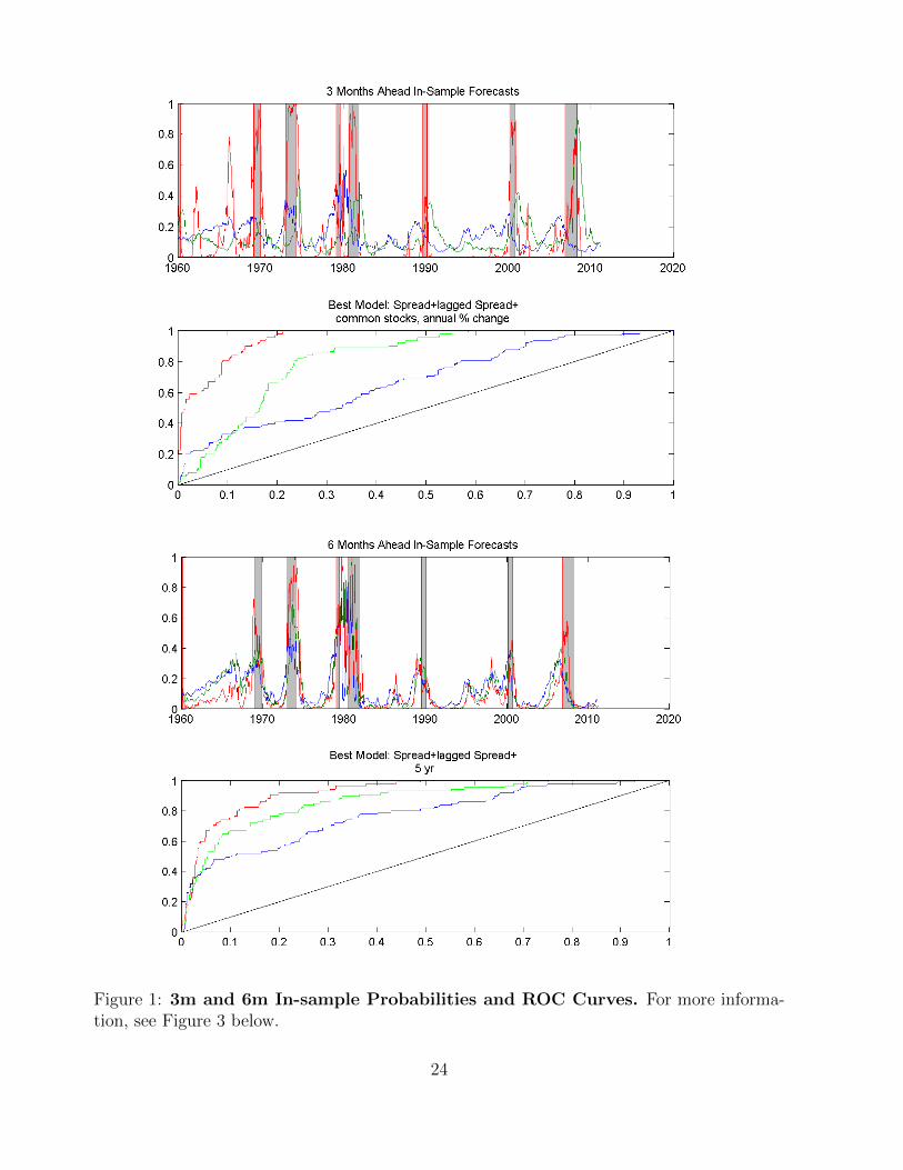
Figure 1: 3m and 6m In-sample Probabilities and ROC Curves. For more informa-tion, see Figure 3 below.

24

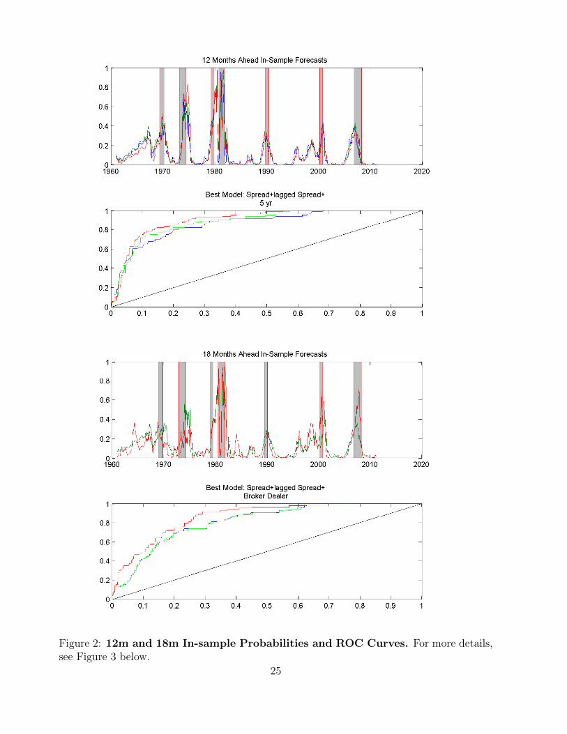
Figure 2: 12m and 18m In-sample Probabilities and ROC Curves. For more details,see Figure 3 below.

25

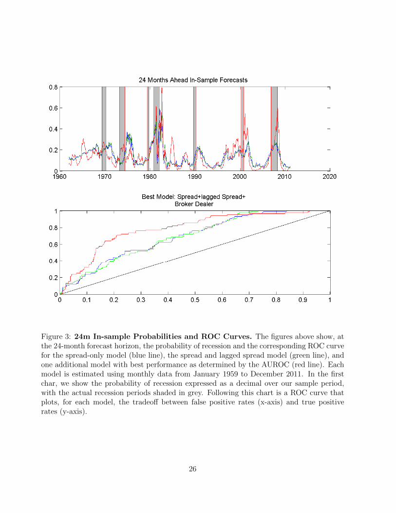
Figure 3: 24m In-sample Probabilities and ROC Curves. The figures above show, atthe 24-month forecast horizon, the probability of recession and the corresponding ROC curvefor the spread-only model (blue line), the spread and lagged spread model (green line), andone additional model with best performance as determined by the AUROC (red line). Eachmodel is estimated using monthly data from January 1959 to December 2011. In the firstchar, we show the probability of recession expressed as a decimal over our sample period,with the actual recession periods shaded in grey. Following this chart is a ROC curve thatplots, for each model, the tradeoff between false positive rates (x-axis) and true positiverates (y-axis).

26

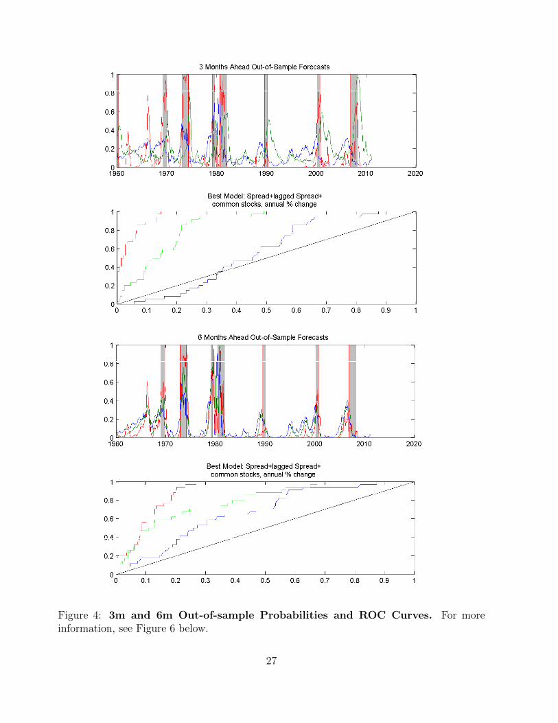
Figure 4: 3m and 6m Out-of-sample Probabilities and ROC Curves. For moreinformation, see Figure 6 below.

27

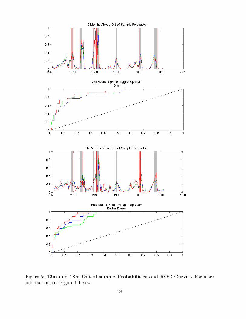
Figure 5: 12m and 18m Out-of-sample Probabilities and ROC Curves. For moreinformation, see Figure 6 below.

28

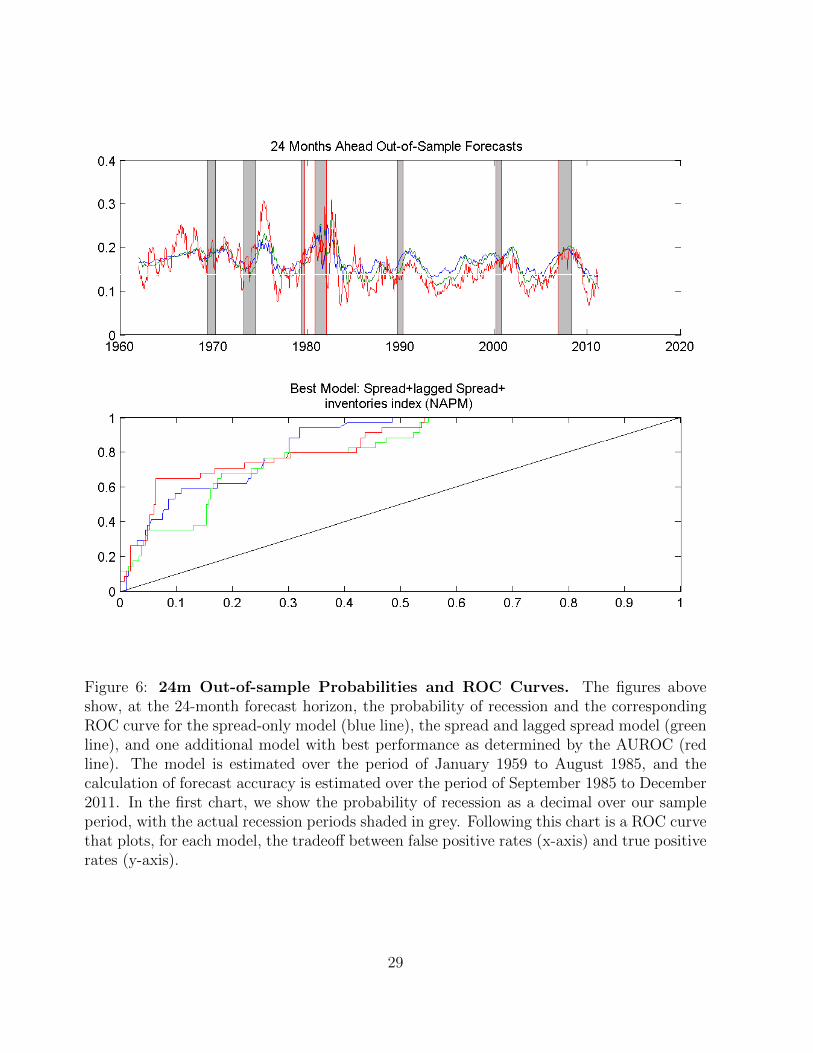
Figure 6: 24m Out-of-sample Probabilities and ROC Curves. The figures aboveshow, at the 24-month forecast horizon, the probability of recession and the correspondingROC curve for the spread-only model (blue line), the spread and lagged spread model (greenline), and one additional model with best performance as determined by the AUROC (redline). The model is estimated over the period of January 1959 to August 1985, and thecalculation of forecast accuracy is estimated over the period of September 1985 to December2011. In the first chart, we show the probability of recession as a decimal over our sampleperiod, with the actual recession periods shaded in grey. Following this chart is a ROC curvethat plots, for each model, the tradeoff between false positive rates (x-axis) and true positiverates (y-axis).

29

References

Adrian, T., E. Etula, and T. Muir (2012): “Financial intermediaries and the cross-

section of asset returns,” Journal of Finance, forthcoming.

Adrian, T., E. Moench, and H. S. Shin (2010): “Macro risk premium and intermediary

balance sheet quantities,” IMF Economic Review, 58(1), 179–207.

(2013): “Leverage asset pricing,” Staff Reports 625, Federal Reserve Bank of New

York.

Adrian, T., and H. S. Shin (2010): “Liquidity and leverage,” Journal of Financial In-

termediation, 19(3), 418–437.

Berge, T. J., and O. Jorda (2011): “Evaluating the classification of economic activity

into recessions and expansions,” American Economic Journal: Macroeconomics, 3(2), 246–

277.

Chauvet, M., and S. Potter (2005): “Forecasting recessions using the yield curve,”

Journal of Forecasting, 24(2), 77–103.

Chesher, A. (1984): “Improving the efficiency of probit estimators,” The Review of Eco-

nomics and Statistics, 66, 523–527.

Conniffe, D., and D. O’Neill (2011): “Efficient Probit Estimation with Partially Miss-

ing Covariates,” Advances in Econometrics, 27, 209–245.

Croushore, D., and K. Marsten (2014): “The continuing power of the yield spread in

forecasting recessions,” Working Papers 14-5, Federal Reserve Bank of Philadelphia.

Duarte, A., I. A. Venetis, and I. Paya (2005): “Predicting real growth and the prob-

ability of recession in the Euro area using the yield spread,” International Journal of

Forecasting, 21(2), 261–277.

30

Dueker, M. J. (1997): “Strengthening the case for the yield curve as a predictor of U.S.

recessions,” St. Louis Fed Review, (Mar), 41–51.

Estrella, A., and G. A. Hardouvelis (1991): “The term structure as a predictor of

real economic activity,” The Journal of Finance, 46(2), 555–576.

Estrella, A., and F. S. Mishkin (1996): “The yield curve as a predictor of U.S. reces-

sions,” Current Issues in Economics and Finance, 2(7), 1–6.

(1998): “Predicting U.S. recessions: Financial variables as leading indicators,” The

Review of Economics and Statistics, 80(1), 45–61.

Estrella, A., and M. R. Trubin (2006): “The yield curve as a leading indicator: Some

practical issues,” Current Issues in Economics and Finance, 12(5), 1–7.

Hanley, J. A., and B. J. McNeil (1982): “The meaning and use of the area under a

receiver operating characteristic (ROC) curve,” Radiology, 143(1), 29–36.

(1983): “A method of comparing the areas under receiver operating characteristic

curves derived from the same cases,” Radiology, 148(3), 839–843.

Jorda, O., and A. M. Taylor (2011): “Performance evaluation of zero net-investment

strategies,” Discussion paper, National Bureau of Economic Research.

(2012): “The carry trade and fundamentals: Nothing to fear but FEER itself,”

Journal of International Economics, 88(1), 74–90.

Khandani, A. E., A. J. Kim, and A. W. Lo (2010): “Consumer credit risk models via

machine-learning algorithms,” Journal of Banking & Finance, 34(11), 2767–2787.

Lahiri, K., G. Monokroussos, and Y. Zhao (2013): “The yield spread puzzle and the

information content of SPF forecasts,” Economics Letters, 118(1), 219–221.

31

Levanon, G., J.-C. Manini, A. Ozyildirim, B. Schaitkin, and J. Tanchua (2011):

“Using a leading credit index to predict turning points in the U.S. business cycle,” Eco-

nomics Program Working Papers 11-05, The Conference Board, Economics Program.

Moore, G. H., and J. Shiskin (1967): Indicators of Business Expansions and Contrac-

tions, NBER Books. National Bureau of Economic Research.

Ng, S. (2014): “Viewpoint: Boosting recessions,” Canadian Journal of Economics, 47(1),

1–34.

Nyberg, H. (2010): “Dynamic probit models and financial variables in recession forecast-

ing,” Journal of Forecasting, 29(1-2), 215–230.

Peterson, W. W., and T. G. Birdsall (1953): “The Theory of Signal Detectability:

Part I. The General Theory,” Technical Report 13, Electronic Defense Group.

Rudebusch, G. D., and J. C. Williams (2009): “Forecasting recessions: The puzzle of

the enduring power of the yield curve,” Journal of Business & Economic Statistics, 27(4),

492–503.

Schrimpf, A., and Q. Wang (2010): “A reappraisal of the leading indicator properties of

the yield curve under structural instability,” International Journal of Forecasting, 26(4),

836–857.

Stock, J. H., and M. W. Watson (1989): “New indexes of coincident and leading

economic indicators,” in NBER Macroeconomics Annual 1989, Volume 4, NBER Chapters,

pp. 351–409. National Bureau of Economic Research, Inc.

Wright, J. H. (2006): “The yield curve and predicting recessions,” Discussion paper,

Board of Governors of the Federal Reserve System.

32