What makes an artist? The evolution and clustering of

What makes an artist? The evolution and

clustering of creative activity in the US since 1850

by

Karol Jan Borowiecki and Christian Møller Dahl

Discussion Papers on Business and Economics

No. 1/2021

FURTHER INFORMATION

Department of Business and Economics

Faculty of Business and Social Sciences

University of Southern Denmark

Campusvej 55, DK-5230 Odense M

Denmark

ISSN 2596-8157 E-mail: [email protected] / http://www.sdu.dk/ivoe

What makes an artist? The evolution andclustering of creative activity in the US since 1850

Karol Jan Borowiecki∗1 and Christian Møller Dahl2

1Historical Economics and Development Group (HEDG),Department of Business and Economics, University of Southern

Denmark2Department of Business and Economics, University of Southern

Denmark

January 20, 2021

Abstract: This research illuminates the historical development and clustering ofcreative activity in the United States. Census data is used to identify creative occu-pations (i.e., artists, musicians, authors, actors) and data on prominent creatives, aslisted in a comprehensive biographical compendium. The analysis first sheds lighton the socio-economic background of creative people and how it has changed since1850. The results indicate that the proportion of female creatives is relatively high,time constraints can be a hindrance for taking up a creative occupation, racial in-equality is present and tends to change only slowly, and access to financial resourceswithin a family facilitates the uptake of an artistic occupation. Second, the studysystematically documents and quantifies the geography of creative clusters in theUnited States and explains how these have evolved over time and across creativedomains.

Keywords: Creativity, artists, geographic clustering, agglomeration economies, ur-ban history.

JEL Classification Numbers: R1, N33, Z11.

∗Corresponding author Karol J. Borowiecki: [email protected]. This paper has been disseminatedpreviously under the title ”The Origins of Creativity: The Case of the Arts in the United Statessince 1850”. The authors wish to thank Philipp Ager, David de la Croix, Walker Hanlon, NathanNunn, Casper Worm Hansen, and participants at the World Economic History Congress (Kyoto),Interdisciplinary Conference on Art Markets (Amsterdam), Workshop on Growth, History andDevelopment (Odense), Economic History and Economic Policy Conference (Paris), FRESH Meet-ing (Odense), European Workshop on Applied Cultural Economics (Vienna), SOUND EconomicHistory Workshop (Lund) and invited seminar at Syddansk Universitet Sønderborg for helpfulconsultations and insightful comments. Outstanding research assistance was provided by MartinHørlyk Kristensen. This research has been co-funded by the Danish Research Council under theproject ”Origins of Creativity”.

1

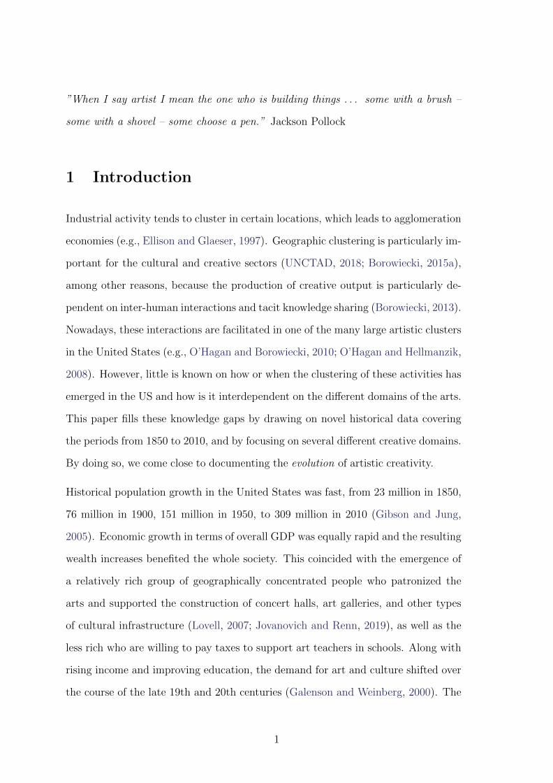
”When I say artist I mean the one who is building things . . . some with a brush –

some with a shovel – some choose a pen.” Jackson Pollock

1 Introduction

Industrial activity tends to cluster in certain locations, which leads to agglomeration

economies (e.g., Ellison and Glaeser, 1997). Geographic clustering is particularly im-

portant for the cultural and creative sectors (UNCTAD, 2018; Borowiecki, 2015a),

among other reasons, because the production of creative output is particularly de-

pendent on inter-human interactions and tacit knowledge sharing (Borowiecki, 2013).

Nowadays, these interactions are facilitated in one of the many large artistic clusters

in the United States (e.g., O’Hagan and Borowiecki, 2010; O’Hagan and Hellmanzik,

2008). However, little is known on how or when the clustering of these activities has

emerged in the US and how is it interdependent on the different domains of the arts.

This paper fills these knowledge gaps by drawing on novel historical data covering

the periods from 1850 to 2010, and by focusing on several different creative domains.

By doing so, we come close to documenting the evolution of artistic creativity.

Historical population growth in the United States was fast, from 23 million in 1850,

76 million in 1900, 151 million in 1950, to 309 million in 2010 (Gibson and Jung,

2005). Economic growth in terms of overall GDP was equally rapid and the resulting

wealth increases benefited the whole society. This coincided with the emergence of

a relatively rich group of geographically concentrated people who patronized the

arts and supported the construction of concert halls, art galleries, and other types

of cultural infrastructure (Lovell, 2007; Jovanovich and Renn, 2019), as well as the

less rich who are willing to pay taxes to support art teachers in schools. Along with

rising income and improving education, the demand for art and culture shifted over

the course of the late 19th and 20th centuries (Galenson and Weinberg, 2000). The

1

change has been visible in numerous dimensions and in the exploration that follows

we will document in particular a rapid increase in the number of artists and the rise

in the diversity of artistic occupations.

High skilled people generate ideas (Glaeser, 2003) and their presence is correlated

with city growth (e.g., Glaeser, 1994; Gergaud et al., 2016). Urban development

comes from being an attractive “consumer city” for high skill people (Glaeser et al.,

2001) and the presence of creative people, in particular of artists, may enhance this

attractiveness (e.g., Florida, 2002). Creative and arts sectors are seen as ”the key

ingredient for job creation, innovation and trade” (UNCTAD, 2010) and are believed

to constitute opportunities for developing countries to leapfrog into emerging high-

growth areas of the world economy. Creativity is potentially ”driving the economy,

reshaping entire industries and stimulating inclusive growth” (OECD, 2014). As can

be seen in Figure 1, the correlation between the density of creative people and startup

activity in US cities is surprisingly strong, also in the long run.1 Finally, artistic

creativity is needed to produce cultural goods and services, and the advantages

of having a wealthy cultural supply and a meaningful cultural heritage nowadays

are vast and non-negligible, ranging from economic gains from tourism inflows to

non-monetary gains arising from a common identity.

Despite the remarkable importance of artistic creativity, economists have largely

refrained from studying it. Creativity in the arts is explored even less by economic

historians, especially since creativity is not a characteristic that has been priced

highly on labor markets throughout most of history. In the past, employers have

valued disciplined and hard-working workers (Crafts, 1985), as opposed to creative

ones. Our focus is directed on the arts, which incorporate some of the earliest

1Even if simple scatter plots are subject to biases due to unobservable factors (e.g., educationalattainment), the strength of the disclosed correlation is rather striking. Causal claims cannot bemade, but improved opportunities to consume cultural goods such as theater (Glaeser et al., 2001)or the presence of cultural amenities (Falck et al., 2018) are an important factor in the locationdecision of high-skilled workers - and are likely related with the density of creatives. See alsoGlaeser et al. (2010) for a summary of the local causes and consequences of entrepreneurship.

2

Atlanta, GA

Austin, TX

Baltimore, MD

Boston, MA

Charlotte, NC

Chicago, IL

Cincinnati, OHCleveland, OH

Columbus, OH

Denver, CO

Detroit, MI

Houston, TX

Indianapolis, IN

Jacksonville, FLKansas City, MO-KS

Las Vegas, NV

Los Angeles, CA

Miami, FL

Milwaukee, WI

Minneapolis, MN

Nashville, TN

New York, NY

Orlando, FL

Philadelphia, PA

Phoenix, AZ

Pittsburgh, PA

Portland, OR

Providence, RI

Riverside, CA Sacramento, CASan Antonio, TX

San Diego, CA

San Francisco, CA

San Jose, CA

Seattle, WA

St. Louis, MO

Virginia Beach, VA

Washington, DC

510

1520

Cre

ativ

es D

ensi

ty, 1

850-

2010

1 1.5 2 2.5 3Startup Density, 1980-2010

Figure 1. Creatives and Startup Densities (per 1000 people). Sources: IPUMS(2015), Fairlie et al. (2015). Note: Creatives include artists, musicians, authors,and actors.

creative occupations. Therefore, this study may provide some unique insights on the

long-term development, geographic spread, and individual motivations to engage in

creative activity.2

This research is mostly descriptive and does not support any causal claims. Nonethe-

less, it makes three main contributions. First, we shed light on the determinants of a

person engaging in an artistic occupation by using individual-level data. These anal-

yses illuminate how the socio-economic profiles of artists have changed since 1850,

thereby delivering unique insights into long-term patterns of artistic occupational

choices. The focus is directed on individuals representing the visual arts, literary

arts and performing arts, and music. The chosen categories are in line with the

definition of traditional high art by Heilbrun and Gray (2001). Furthermore, by

2In the remainder of the paper by referring to creativity or creative people, what is meant isartistic creativity and artists, albeit artistic creativity is likely correlated with the same variables asis the sort of creativity that leads to innovation in production and economic growth. For example,within psychology, artistic, scientific or entrepreneurial creativity is studied along side each other(e.g., Ludwig, 1995), albeit in different contexts.

3

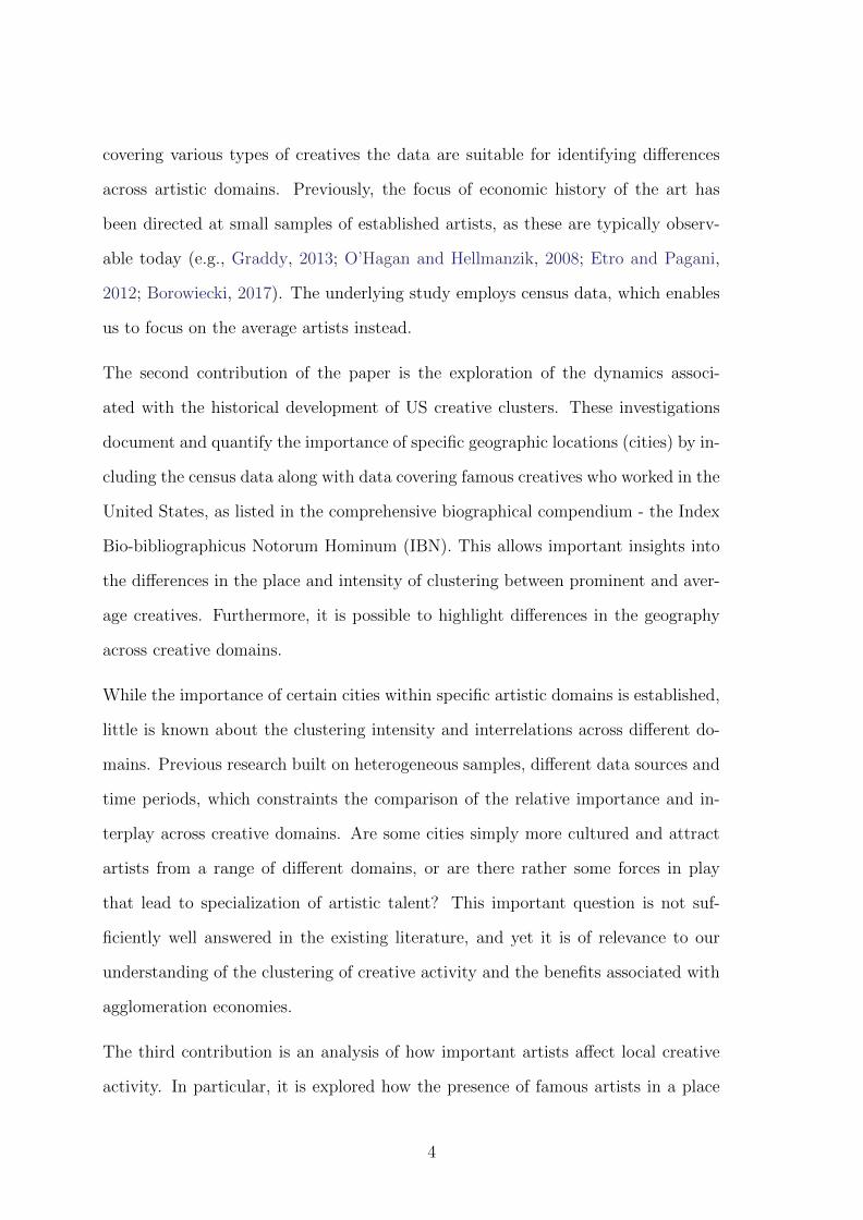
covering various types of creatives the data are suitable for identifying differences

across artistic domains. Previously, the focus of economic history of the art has

been directed at small samples of established artists, as these are typically observ-

able today (e.g., Graddy, 2013; O’Hagan and Hellmanzik, 2008; Etro and Pagani,

2012; Borowiecki, 2017). The underlying study employs census data, which enables

us to focus on the average artists instead.

The second contribution of the paper is the exploration of the dynamics associ-

ated with the historical development of US creative clusters. These investigations

document and quantify the importance of specific geographic locations (cities) by in-

cluding the census data along with data covering famous creatives who worked in the

United States, as listed in the comprehensive biographical compendium - the Index

Bio-bibliographicus Notorum Hominum (IBN). This allows important insights into

the differences in the place and intensity of clustering between prominent and aver-

age creatives. Furthermore, it is possible to highlight differences in the geography

across creative domains.

While the importance of certain cities within specific artistic domains is established,

little is known about the clustering intensity and interrelations across different do-

mains. Previous research built on heterogeneous samples, different data sources and

time periods, which constraints the comparison of the relative importance and in-

terplay across creative domains. Are some cities simply more cultured and attract

artists from a range of different domains, or are there rather some forces in play

that lead to specialization of artistic talent? This important question is not suf-

ficiently well answered in the existing literature, and yet it is of relevance to our

understanding of the clustering of creative activity and the benefits associated with

agglomeration economies.

The third contribution is an analysis of how important artists affect local creative

activity. In particular, it is explored how the presence of famous artists in a place

4

are related to the probability of an individual becoming involved in a creative oc-

cupation. By making use of census data that reflect the creative involvement of

average individuals, as opposed to prominent ones, it is possible to overcome the

extreme non-random sample selection biases encountered in the fast growing related

literature (e.g., O’Hagan and Borowiecki, 2010).

2 Literature Review

This research primarily relates to four strands of the literature. First, this paper

builds on literature on human capital theory of city growth by analysing how human

capital accumulates across cities and over time. The focus on creative people only

comes close to what Florida (2002) describes as the creative class, but the paper

in its essence is about human capital formation in agglomerations (Glaeser, 2004).

Natural advantage plays a role in the formation of agglomerations and firms show a

higher clustering intensity than they would be if they were randomly located (Ellison

and Glaeser, 1997; Duranton and Overman, 2005). New economic geography models

suggest that transportation costs induce people and firms to cluster in cities (Fujita

et al., 1999). Cities and industries that cluster are associated with higher wages

and prices (Rosenthal and Strange, 2004; Puga, 2010), and hence clusters must

experience some kind of advantages to be competitive (Ellison and Glaeser, 1999).

These advantages take different forms in different times. For example, at the turn of

the 20th century it may have mattered to be close to a coal mine or the harbor, but

is not anymore nowadays. Similarly, advantageous climatic conditions have likely

influenced the location for the movie industry in Hollywood, but possibly play a

smaller role nowadays.

The second related strand focuses on the geographic concentration of artistic activity.

Artists exhibit remarkable clustering patterns, both in terms of birth and migration.

5

The predominant location for visual artists born in the first half of the 20th century

is New York City, with all prominent American artists clustering there (O’Hagan

and Hellmanzik, 2008). New York is also a major work location for music composers:

It is the fifth most important city for composers born in the 19th century and, after

Paris, the second most popular destination for 20th century composers (O’Hagan

and Borowiecki, 2010; Borowiecki and O’Hagan, 2012). Globally, Paris was the

predominant music center over a remarkably long period of around four centuries

and this was due to its large size (Borowiecki, 2015a). However, the incidence of the

second World War caused a significant negative shock that led to massive relocations

from the French capital to New York City. Borowiecki and Graddy (2018) find that

US cities that experience larger immigrant artist inflows also see a greater inflow of

native artists. In a more contemporary setting, Andersen (2014) show that location

choices of artists are driven by access to other artists and by consumer demand.

Geographic clustering of creative activity is also associated with strong productivity

gains (e.g., Tao, 2019). It has been shown that literary artists born between 1750

and 1925 experienced significant productivity gains when working in London, the

predominant cluster within literary arts (Mitchell, 2019). Visual artists born 1850 to

1945 peaked earlier in the geographic clusters of Paris and New York (Hellmanzik,

2010). Music composers born in the late 18th and 19th centuries were more produc-

tive in the main hubs for music (Borowiecki, 2013) and the benefits increased with

the peer group size at a decreasing rate (Borowiecki, 2015a). The focus in these

studies is, however, on selected, specific artistic domains, and while interdisciplinary

spillovers are sometimes acknowledged (e.g., Borowiecki, 2013, describes how com-

posers in Paris have been in contact with literary and visual artists), little is known

about how these domains interrelate or interlocate.

Third, this research relates to the literature on the attractiveness of cities. Urban

development takes particularly place in cities that facilitate consumption for high

6

skill people, and hence a “consumer city” is thriving more (Glaeser et al., 2001). The

presence of cultural amenities facilitates such consumption and hence attracts high-

skilled workers (e.g., Falck et al., 2018), which then in turn leads to various positive

spillovers. Clustering of creative activity in cities may also have long-term effects

on economic development, including increased innovation activity in certain areas

(Knudsen et al., 2008) or persistent income differences across regions Maloney and

Caicedo (2014). The underlying research does not explicitly address the question

of the consequences of cultural activity. Nonetheless, it outlines the dynamics and

geography of emerging or established creative clusters, and hence provides important

insights into the attractiveness of cities. These insights may have some relevance

considering how cultural developments are correlated with start-up activity (see

Figure 1) and the need for further research on the local causes and consequences of

entrepreneurship (Glaeser et al., 2010).

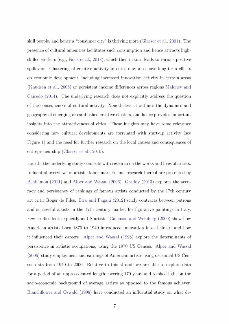
Fourth, the underlying study connects with research on the works and lives of artists.

Influential overviews of artists’ labor markets and research thereof are presented by

Benhamou (2011) and Alper and Wassal (2006). Graddy (2013) explores the accu-

racy and persistency of rankings of famous artists conducted by the 17th century

art critic Roger de Piles. Etro and Pagani (2012) study contracts between patrons

and successful artists in the 17th century market for figurative paintings in Italy.

Few studies look explicitly at US artists. Galenson and Weinberg (2000) show how

American artists born 1870 to 1940 introduced innovation into their art and how

it influenced their careers. Alper and Wassal (1998) explore the determinants of

persistence in artistic occupations, using the 1970 US Census. Alper and Wassal

(2006) study employment and earnings of American artists using decennial US Cen-

sus data from 1940 to 2000. Relative to this strand, we are able to explore data

for a period of an unprecedented length covering 170 years and to shed light on the

socio-economic background of average artists as opposed to the famous achiever.

Blanchflower and Oswald (1998) have conducted an influential study on what de-

7

terminants enhance people to become entrepreneurs, viewed contemporaneously as

”popular hereos” (Blanchflower and Oswald, 1998, opening quote). About 20 years

later the creative artist is increasingly often regarded as the new champion and even

though the traits required by entrepreneurs and artists are in many regards similar,

a study of what makes an artist becomes particularly meaningful.

3 Data

There are two main databases used here. First, we use US census data from the

Integrated Public Use Microdata Series database IPUMS (2015). This comprehen-

sive decennial population census was first undertaken in 1790, but only provides

information from 1850 on occupational status (OCC1950 ), along with a wide array

of background variables. The occupation variable is used in order to identify the

following creatives: Artists and art teachers, authors, musicians and music teachers,

and actors and actresses.3 The occupation categories of artists and musicians also

include the teachers within these domains. This is not necessarily a shortcoming,

since also the presence of art teachers (be it in music or visual arts) serves as a proxy

for creative activity. In places with more art teachers, more artists are educated and

a higher population of artists can be expected, which in consequence leads to greater

artistic activity and creativity (Ateca-Amestoy et al., 2017). The possible overrepre-

sentation of teachers is nonetheless addressed econometrically in the results section,

where we also control for the geographic spread of teachers.

The social setting or technical content of artistic occupations has likely changed over

a period of one and a half centuries. Nonetheless, larger occupational groupings are

3The records also make it possible to identify architects, dancers and dancing teachers, andeditors and reporters. However, these occupations are very rare and deliver an insufficiently lownumber of observations, especially in the earlier periods. In analogy to creative occupations,we will refer to non-creative occupations when writing about occupations other than those ofartists, musicians, authors, and actors. This is done merely for convenience, as opposed to thecategorization of occupations into those that require or do not require creative talent.

8

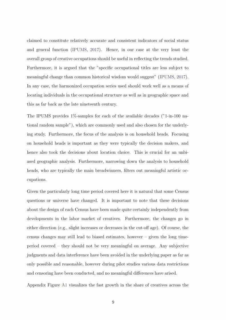
claimed to constitute relatively accurate and consistent indicators of social status

and general function (IPUMS, 2017). Hence, in our case at the very least the

overall group of creative occupations should be useful in reflecting the trends studied.

Furthermore, it is argued that the ”specific occupational titles are less subject to

meaningful change than common historical wisdom would suggest” (IPUMS, 2017).

In any case, the harmonized occupation series used should work well as a means of

locating individuals in the occupational structure as well as in geographic space and

this as far back as the late nineteenth century.

The IPUMS provides 1%-samples for each of the available decades (”1-in-100 na-

tional random sample”), which are commonly used and also chosen for the underly-

ing study. Furthermore, the focus of the analysis is on household heads. Focusing

on household heads is important as they were typically the decision makers, and

hence also took the decisions about location choice. This is crucial for an unbi-

ased geographic analysis. Furthermore, narrowing down the analysis to household

heads, who are typically the main breadwinners, filters out meaningful artistic oc-

cupations.

Given the particularly long time period covered here it is natural that some Census

questions or universe have changed. It is important to note that these decisions

about the design of each Census have been made quite certainly independently from

developments in the labor market of creatives. Furthermore, the changes go in

either direction (e.g., slight increases or decreases in the cut-off age). Of course, the

census changes may still lead to biased estimates, however – given the long time-

period covered – they should not be very meaningful on average. Any subjective

judgments and data interference have been avoided in the underlying paper as far as

only possible and reasonable, however during pilot studies various data restrictions

and censoring have been conducted, and no meaningful differences have arised.

Appendix Figure A1 visualizes the fast growth in the share of creatives across the

9

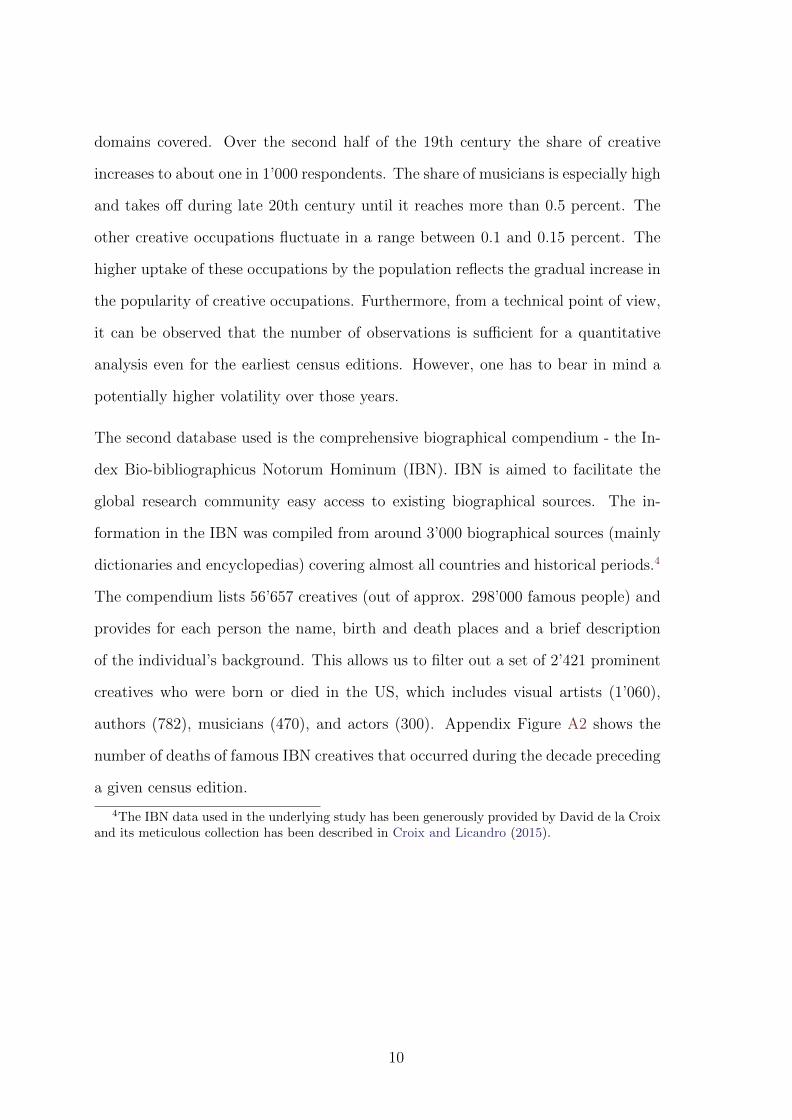
domains covered. Over the second half of the 19th century the share of creative

increases to about one in 1’000 respondents. The share of musicians is especially high

and takes off during late 20th century until it reaches more than 0.5 percent. The

other creative occupations fluctuate in a range between 0.1 and 0.15 percent. The

higher uptake of these occupations by the population reflects the gradual increase in

the popularity of creative occupations. Furthermore, from a technical point of view,

it can be observed that the number of observations is sufficient for a quantitative

analysis even for the earliest census editions. However, one has to bear in mind a

potentially higher volatility over those years.

The second database used is the comprehensive biographical compendium - the In-

dex Bio-bibliographicus Notorum Hominum (IBN). IBN is aimed to facilitate the

global research community easy access to existing biographical sources. The in-

formation in the IBN was compiled from around 3’000 biographical sources (mainly

dictionaries and encyclopedias) covering almost all countries and historical periods.4

The compendium lists 56’657 creatives (out of approx. 298’000 famous people) and

provides for each person the name, birth and death places and a brief description

of the individual’s background. This allows us to filter out a set of 2’421 prominent

creatives who were born or died in the US, which includes visual artists (1’060),

authors (782), musicians (470), and actors (300). Appendix Figure A2 shows the

number of deaths of famous IBN creatives that occurred during the decade preceding

a given census edition.

4The IBN data used in the underlying study has been generously provided by David de la Croixand its meticulous collection has been described in Croix and Licandro (2015).

10

4 Results

4.1 The socio-economic background of creatives since 1850

This section presents the socio-economic background of the creatives covered by

applying a simple regression model as summarized by Equation 1. In particular, a

linear probability model (LPM) is estimated to explore how being involved in any of

the four creative occupations covered is related to the background of an individual.

The LPM is specified as follows:

yit = α +Xitβ +∑year

fyear,i +∑state

fstate,i + uit, (1)

for t = 1, . . . , T and i = 1, . . . , N . The dependent variable in Equation (1) given

by yit is a binary variable indicating if individual i was in a creative occupation

in census year t. Note that our data is unbalanced in the sense that individuals

are only observed for a limited number of census years. The explanatory variables,

summarized by Xit include a dummy for gender, a quadratic age polynomial, a set of

indicator variables that identify the marital status (single is the baseline category),

the number of own family members in household, the number of own children in the

household and a set of dummy variables that identify the race (white is the baseline

category). Finally, the model accounts for census year fixed effects and state fixed

effects by inclusion of the terms∑

year fyear,i and∑

state fstate,i, respectively. Finally,

uit denotes an idiosyncratic error term.

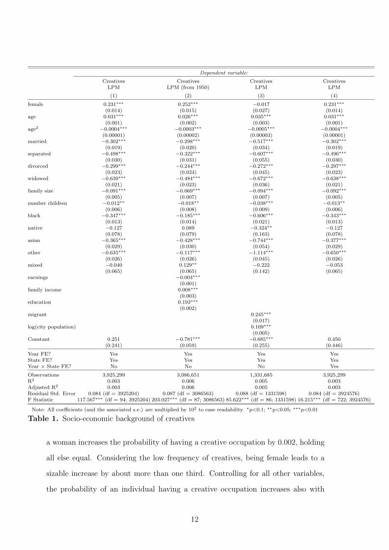
The regression results are reported in Table 1. Most coefficients turn out to be

statistically significant, but since this is co-driven by the high number of observa-

tions, the following interpretation will focus on the direction of the effects. The

magnitudes of the coefficients are in general small, because the average proportion

of people having one of the creative occupations is very low (about 0.0054). Being

11

Dependent variable:

Creatives Creatives Creatives CreativesLPM LPM (from 1950) LPM LPM

(1) (2) (3) (4)

female 0.231∗∗∗ 0.252∗∗∗ −0.017 0.231∗∗∗

(0.014) (0.015) (0.027) (0.014)age 0.031∗∗∗ 0.026∗∗∗ 0.035∗∗∗ 0.031∗∗∗

(0.001) (0.002) (0.003) (0.001)age2 −0.0004∗∗∗ −0.0003∗∗∗ −0.0005∗∗∗ −0.0004∗∗∗

(0.00001) (0.00002) (0.00003) (0.00001)married −0.302∗∗∗ −0.298∗∗∗ −0.517∗∗∗ −0.302∗∗∗

(0.019) (0.020) (0.034) (0.019)separated −0.498∗∗∗ −0.322∗∗∗ −0.607∗∗∗ −0.496∗∗∗

(0.030) (0.031) (0.055) (0.030)divorced −0.299∗∗∗ −0.244∗∗∗ −0.272∗∗∗ −0.297∗∗∗

(0.023) (0.024) (0.045) (0.023)widowed −0.639∗∗∗ −0.484∗∗∗ −0.672∗∗∗ −0.638∗∗∗

(0.021) (0.023) (0.036) (0.021)family size −0.091∗∗∗ −0.069∗∗∗ −0.094∗∗∗ −0.092∗∗∗

(0.005) (0.007) (0.007) (0.005)number children −0.012∗∗ −0.018∗∗ −0.038∗∗∗ −0.013∗∗

(0.006) (0.008) (0.009) (0.006)black −0.347∗∗∗ −0.185∗∗∗ −0.606∗∗∗ −0.343∗∗∗

(0.013) (0.014) (0.021) (0.013)native −0.127 0.089 −0.324∗∗ −0.127

(0.078) (0.079) (0.163) (0.078)asian −0.365∗∗∗ −0.428∗∗∗ −0.744∗∗∗ −0.377∗∗∗

(0.029) (0.030) (0.054) (0.029)other −0.635∗∗∗ −0.117∗∗∗ −1.114∗∗∗ −0.650∗∗∗

(0.026) (0.026) (0.045) (0.026)mixed −0.040 0.129∗∗ −0.222 −0.053

(0.065) (0.065) (0.142) (0.065)earnings −0.004∗∗∗

(0.001)family income 0.008∗∗∗

(0.003)education 0.193∗∗∗

(0.002)migrant 0.245∗∗∗

(0.017)log(city population) 0.109∗∗∗

(0.005)Constant 0.251 −0.781∗∗∗ −0.685∗∗∗ 0.450

(0.241) (0.059) (0.255) (0.446)

Year FE? Yes Yes Yes YesState FE? Yes Yes Yes YesYear × State FE? No No No Yes

Observations 3,925,299 3,086,651 1,331,685 3,925,299R2 0.003 0.006 0.005 0.003Adjusted R2 0.003 0.006 0.005 0.003Residual Std. Error 0.084 (df = 3925204) 0.087 (df = 3086563) 0.088 (df = 1331598) 0.084 (df = 3924576)F Statistic 117.567∗∗∗ (df = 94; 3925204) 203.027∗∗∗ (df = 87; 3086563) 85.622∗∗∗ (df = 86; 1331598) 16.215∗∗∗ (df = 722; 3924576)

Note: All coefficients (and the associated s.e.) are multiplied by 102 to ease readability. ∗p<0.1; ∗∗p<0.05; ∗∗∗p<0.01

Table 1. Socio-economic background of creatives

a woman increases the probability of having a creative occupation by 0.002, holding

all else equal. Considering the low frequency of creatives, being female leads to a

sizable increase by about more than one third. Controlling for all other variables,

the probability of an individual having a creative occupation increases also with

12

age, but at a decreasing rate. The results show also that those who are married,

separated, divorced or widowed are less likely to take up a creative occupation than

singles. Personal commitment, approximated by family size and number of children,

are also negatively related with having an artistic occupation. On average, the black

and Asian groups are less likely to engage in creative work than whites.

The baseline model (Equation 1) is then extended by education and income variables.

Educational attainment, which is available from 1940, is measured on an ordinal scale

between zero and 11, as described previously. Income is measured in two ways. First,

the model includes labor only income (earnings), which is measured as the total pre-

tax wage and salary income for the previous year and is available from 1940. This

variable captures the effects of an artists’ remuneration and hence is directly related

to the financial incentives of choosing a creative occupation. Second, the model takes

account of total family income, which is measured as the total pre-tax money income

earned by one’s family from all sources for the previous year, including non-labor

income. This variable is available from 1950 and its inclusion is motivated by the

fact that the participation decision depends likely not only on one’s own earnings,

but on the total income of the family. Both income variables have been adjusted for

inflation and are logged.

Column (2) of Table 1 summarizes the results. It can be observed that better ed-

ucation increases the probability of a person having a creative occupation. On the

other hand, earnings are negatively related with creative occupations — an associa-

tion that is often found for creative workers, who typically earn less than the average

(e.g., Alper and Wassal, 2006). Or from another perspective: The low earnings of

artists are detrimental to taking up of an artistic occupations. Interestingly, total

family income exhibits a positive relation with the uptake of a creative occupation.

This is in line with the notion that potential access to family’s financial support is a

factor conducive in the participation decision. Having access to financial resources

13

facilitates the uptake of a creative occupation and the associated lower earnings and

potentially higher uncertainties.

The baseline model is further extended by the inclusion of controls for migrants

and logged city population. In column (3) it can be observed that these additional

controls decrease the number of observations to about 1.3 million (from the initially

almost 4 million observations). The newly added variables indicate that migrants

are more likely to have a creative occupation, as are those who locate in larger

agglomerations. The other previously presented results remain robust.

The background of creatives over time

The regression approach can be complemented with and is supported by a sim-

ple graphical analysis depicting how creatives’ background change over time and

differ across domains. Figure 2 shows the share of females for the four groups of

creatives studied, along with the share of females engaged in any other occupation

(labeled non-creative occupations). The share of women in non-creative occupations

is around 10% at the beginning of the observation window and gradually increases

to around 40% by 2010. This corresponds with the overall labor force participation

of women (e.g., Goldin, 2006, Figure 1). During most of the second half of the 19th

century relatively fewer female are involved in creative occupations than in other

occupations. However, this changes from around 1890 when the share of females

increases sharply and remains clearly above non-creative occupations before the two

trends converge around 1980 for most domains.

These results challenge the conventional wisdom that the arts are predominantly a

male only domain. For example, previous research - which is based on prominent

creatives - shows that women are practically unobservable among famous artists

(e.g., O’Hagan and Borowiecki, 2010; Hellmanzik, 2010). In contrast, by looking

at the average artist, as recorded by the census data, it can be seen that women

14

0.2

.4.6

Fem

ale

shar

e by

occ

upat

ion

1850 1900 1950 2000Census year

Artist MusicianAuthor ActorNon-creatives

Figure 2. Female share by occupation. Note: The ”Non-creatives” categoryprovides the average for all occupations other than the four creative occupationslisted here.

have often been involved in creative occupations and that their share in these oc-

cupations - relative to males - has typically been higher than in non-creative ones.

The observed patterns are also reflected anecdotally in various events that occurred

in the American arts education landscape. For example, the Art Students League,

founded in 1875 in New York City, saw an increasing number of women artists from

the early 1890s (Weber, 2012).

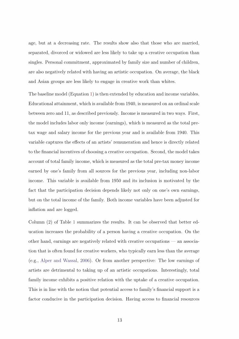
Turning next to age differences, we can observe in Figure 3 that creative occupations

are typically exercised by younger cohorts. One possible explanation for this is that

older cohorts drop out from artistic occupations; however, the cross-section data used

do not permit the investigation of the reasons behind this result in more depth. The

exception is authors, who until the 1930s are on average up to ten years older than

the average household head. The higher age of literary artists is possibly explained

by their need to acquire a particular stock of cultural capital, before producing a

literary artwork. These writers could also have been experimental innovators, who

15

3540

4550

55Ag

e by

occ

upat

ion

1850 1900 1950 2000Census year


Figure 3. Age by occupation. Note: See Figure 2

achieve success gradually and typically later in their careers (Galenson, 2007).

The results presented in Figure 4 address family background and disclose how the

share of singles in the American population gradually increases from levels below

5% up to about 18% by 2010. The rise in the share of single respondents among

those involved in creative occupations is considerably steeper, and by the end of our

observation window about one in four creatives is single, with actors reaching the

highest proportion of 40%. The opposite is true for the respondents’ family sizes in

Figure A3. Over the last one and a half centuries, a steady decrease from about five

family members to just above 2.5 can be observed. The family size of creatives is

typically by at least one person smaller; however, this difference has decreased over

the most recent 2-3 decades.

The observed overall higher share of singles and smaller family sizes among creatives

is perhaps no surprise. Both variables are related to personal or time constraints

and likely limit the individual’s involvement in creative activities. These results are

in line with the research on cultural participation, which finds very similar patterns

16

0.1

.2.3

.4Si

ngle

sha

re b

y oc

cupa

tion

1850 1900 1950 2000Census year


Figure 4. Being single by occupation. Note: See Figure 2

and attributes them to the time constraints of a person (e.g., Ateca-Amestoy, 2008).

Furthermore, as we will see later, creative occupations are also usually lower paid

than non-creative ones, and hence perhaps their ability to afford to get married or

have a family is limited.

Figure 5 explores racial differences and shows that the share of whites decreases from

98% to around 80% over the time period covered. The figure indicates also that it

takes almost a whole century before the first non-whites appear among artists or

authors. Actors are somewhat less dominated by whites in the early 20th century

and since 1980 the proportion of whites drops dramatically. Musicians are the most

racially mixed group of creatives. This does not come perhaps as a surprise if one

considers genres such as jazz, blues, or funk, all invented, mastered, and typically

performed by blacks. These observations come though with a few shortcomings.

First of all, the earliest two census editions do not include slaves, which means that

the picture provided for 1850 and 1860 is incomplete. Second, non-whites who were

involved in creative artistic activity over the earlier part of the period studied may

17

.8.8

5.9

.95

1Sh

are

of w

hite

by

occu

patio

n

1850 1900 1950 2000Census year


Figure 5. White by occupation. Note: See Figure 2

not have been counted as ”artists” by historical census enumerators. This could be

why it looks like there are no black artists or authors until the mid-20th century.

Given the fact that some of the most important American art forms were created

by African Americans, one needs to be careful in the interpretation of the census

data.

Figure 6 provides insights into the educational attainment of the creatives covered.

The censuses until 1930 provide only a dummy indicator for literacy, as presented

in the left panel of the figure. It can be observed that the vast majority of creatives

are literate and clearly more so than those involved in non-creative occupations.

From 1940 the census data provide a more sophisticated measure of educational

attainment by indicating the level of school accomplishment or the number of college

years completed. Based on this information an ordinal scale between zero and 11

has been compiled and is used in the right panel. The educational attainment is

sharply increasing until about the 1990s when the increase becomes less marked.

As in the pre-1940 period, the creatives have obtained significantly more education

18

.8.8

5.9

.95

1Li

tera

cy b

y oc

cupa

tion

1840 1860 1880 1900 1920 1940Census year


24

68

10Ed

ucat

iona

l atta

inm

ent b

y oc

cupa

tion

1940 1960 1980 2000 2020Census year


Figure 6. Educational attainment by occupation. Note: See Figure 2

than the average non-creative worker. There are also interesting differences across

the creative domains, with authors being the best educated, whereas actors are at

the lower end of education attainment.

Disaggregating by the creative domain

Table 2 provides the baseline results disaggregated by the creative domain. Males are

less likely to be authors or musicians, but somewhat more likely to work as actors.

The other meaningful difference is that the probability of being an actor decreases

with age. This supports the notion that actors, especially in the movie industry,

are predominantly male and typically young. The online appendix presents further

results disaggregated by creative domain for a model with education and income

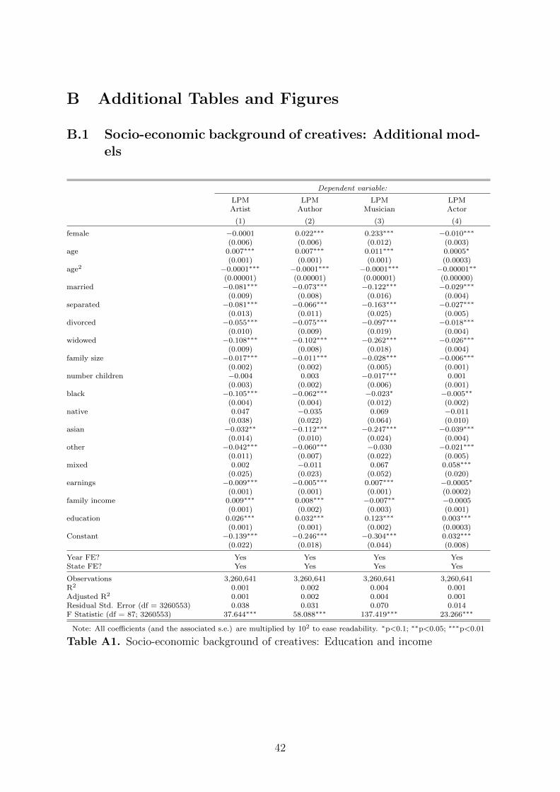
controls (Table A1) and with migrant and city size controls (Table A2).

19

Dependent variable:

LPM LPM LPM LPMArtist Author Musician Actor

(1) (2) (3) (4)

female −0.001 0.021∗∗∗ 0.218∗∗∗ −0.007∗∗∗

(0.006) (0.005) (0.011) (0.003)age 0.007∗∗∗ 0.007∗∗∗ 0.017∗∗∗ 0.0001

(0.001) (0.0005) (0.001) (0.0003)age2 −0.0001∗∗∗ −0.0001∗∗∗ −0.0002∗∗∗ −0.00001∗∗

(0.00001) (0.00000) (0.00001) (0.00000)married −0.080∗∗∗ −0.059∗∗∗ −0.138∗∗∗ −0.025∗∗∗

(0.008) (0.007) (0.015) (0.004)separated −0.101∗∗∗ −0.084∗∗∗ −0.286∗∗∗ −0.026∗∗∗

(0.013) (0.011) (0.025) (0.005)divorced −0.062∗∗∗ −0.076∗∗∗ −0.150∗∗∗ −0.011∗∗

(0.010) (0.008) (0.018) (0.005)widowed −0.131∗∗∗ −0.113∗∗∗ −0.371∗∗∗ −0.025∗∗∗

(0.009) (0.007) (0.017) (0.004)family size −0.020∗∗∗ −0.018∗∗∗ −0.049∗∗∗ −0.005∗∗∗

(0.002) (0.001) (0.004) (0.001)number children −0.004 0.006∗∗∗ −0.011∗∗ −0.004∗∗∗

(0.003) (0.002) (0.005) (0.001)black −0.125∗∗∗ −0.081∗∗∗ −0.131∗∗∗ −0.009∗∗∗

(0.004) (0.004) (0.011) (0.002)native 0.020 −0.067∗∗∗ −0.063 −0.017∗

(0.037) (0.022) (0.064) (0.010)asian −0.025∗ −0.099∗∗∗ −0.199∗∗∗ −0.042∗∗∗

(0.014) (0.009) (0.023) (0.004)other −0.110∗∗∗ −0.139∗∗∗ −0.352∗∗∗ −0.033∗∗∗

(0.011) (0.007) (0.022) (0.005)mixed −0.020 −0.035 −0.037 0.052∗∗∗

(0.025) (0.023) (0.052) (0.020)Constant 0.117 −0.121∗∗ 0.231 0.023∗∗∗

(0.113) (0.057) (0.206) (0.007)

Year FE? Yes Yes Yes YesState FE? Yes Yes Yes Yes

Observations 3,925,299 3,925,299 3,925,299 3,925,299R2 0.001 0.001 0.002 0.001Adjusted R2 0.001 0.001 0.002 0.001Residual Std. Error (df = 3925204) 0.038 0.029 0.067 0.016F Statistic (df = 94; 3925204) 26.045∗∗∗ 36.416∗∗∗ 74.964∗∗∗ 27.504∗∗∗


Table 2. Socio-economic background of creatives by domain

4.2 The historical development of artistic clusters

This section provides historical insights into the geographic clustering patterns of

creative activity in the United States. In the following depictions, the total number

of creatives, as opposed to the share per population, is shown, and there are three

reasons for this. First, it is established that the total number of artists (not the

density) matters for benefits associated with peer effects: Whether artists are based

in a small or large city, the experienced benefits are related to the size of the artist

population (Borowiecki, 2015a). Second, it is more likely that the total number

20

matters more for the attraction of high-skilled workers and possibly for spillover

effects of creativity from the arts to the economic sectors. This is also supported by

the observation that larger cities typically have cultural infrastructures that allow

artists to reach greater audiences (e.g., a larger concert hall). Third, artists usually

cluster in certain districts of a city, and hence considering the population size of a

whole city as a denumerator would be misleading, and an intra-city approach is not

feasible in this research.

Initially, we analyze the geography of artistic talent by looking at the birthplaces and

deathplaces of famous IBN creatives. Even though artists are highly mobile, there

exists a very high correlation between their workplace and birthplace or deathplace.

Furthermore, it is fairly established that the births of famous creatives typically

occur in places where a given artistic domain has already been developed (for evi-

dence and discussion see, for example, O’Hagan and Borowiecki, 2010; Borowiecki

and O’Hagan, 2012).

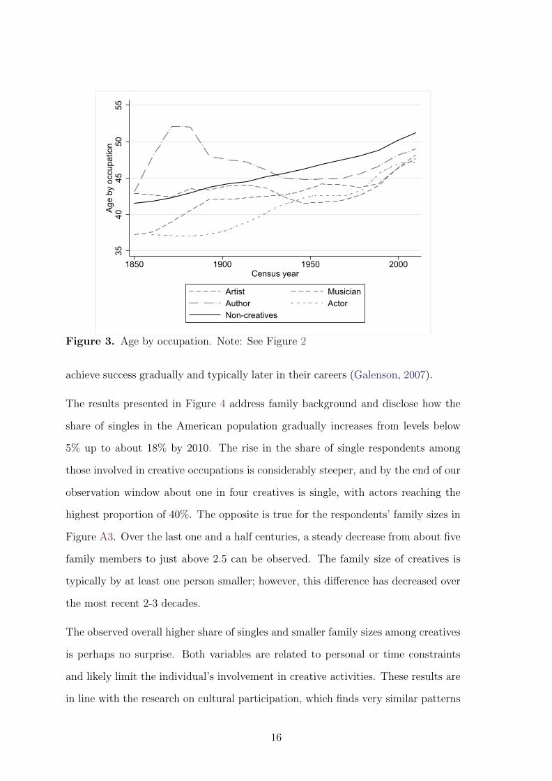
The maps depicting the birthplaces or deathplaces of IBN creatives are presented in

Figures 7 and 8, respectively. Each map indicates by a scaled point the importance of

a city as a birthplace for a certain group of creatives and by shades the importance of

a state.5 Creative activity is primarily located in the Mid Atlantic, North Eastern,

and a part of Mid Western regions, and along the West Coast. The geographic

concentration is more intense for the deathplaces - this supports the previously

posited high migration intensity (both internal migration and immigration). Across

all creative domains studied, New York City emerges as the consistently largest

cluster city, followed by Boston, Chicago, Los Angeles, and San Francisco.6

There are, however, also clear differences across the domains. For example, New

Orleans is found to be a place with a very high concentration of births of musicians.

5For some few observations the exact city was not available, and only information on the countyor state was provided.

6Miami also receives some prominence when it comes to deaths, but this is possibly more relatedto the fact that it is a popular destination for retirement.

21

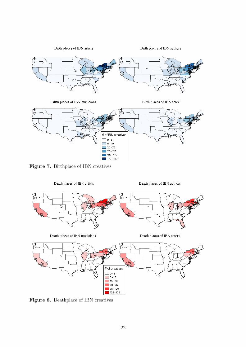
Figure 7. Birthplace of IBN creatives

Figure 8. Deathplace of IBN creatives

22

In New Orleans funk was supposedly played for the first time ever but more impor-

tantly, it is the city where jazz originated. The insight that a significant number

of famous musicians were born here lends support to the colloquial label assigned

to the city as the birthplace of jazz. Another example is St. Louis, a city strongly

associated with blues, but also jazz and ragtime. Interestingly though, while these

two cities emerge as unusually important birthplaces, markedly fewer deaths are ob-

served there. This indicates that many of the famous individuals born here migrated

away. Perhaps the most famous example is Louis Armstrong, who was born in New

Orleans, but died in New York City, where he also spent a significant part of his

career.

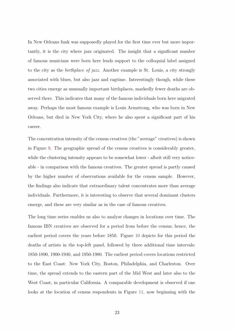
The concentration intensity of the census creatives (the ”average” creatives) is shown

in Figure 9. The geographic spread of the census creatives is considerably greater,

while the clustering intensity appears to be somewhat lower - albeit still very notice-

able - in comparison with the famous creatives. The greater spread is partly caused

by the higher number of observations available for the census sample. However,

the findings also indicate that extraordinary talent concentrates more than average

individuals. Furthermore, it is interesting to observe that several dominant clusters

emerge, and these are very similar as in the case of famous creatives.

The long time series enables us also to analyse changes in locations over time. The

famous IBN creatives are observed for a period from before the census; hence, the

earliest period covers the years before 1850. Figure 10 depicts for this period the

deaths of artists in the top-left panel, followed by three additional time intervals:

1850-1890, 1900-1940, and 1950-1980. The earliest period covers locations restricted

to the East Coast: New York City, Boston, Philadelphia, and Charleston. Over

time, the spread extends to the eastern part of the Mid West and later also to the

West Coast, in particular California. A comparable development is observed if one

looks at the location of census respondents in Figure 11, now beginning with the

23

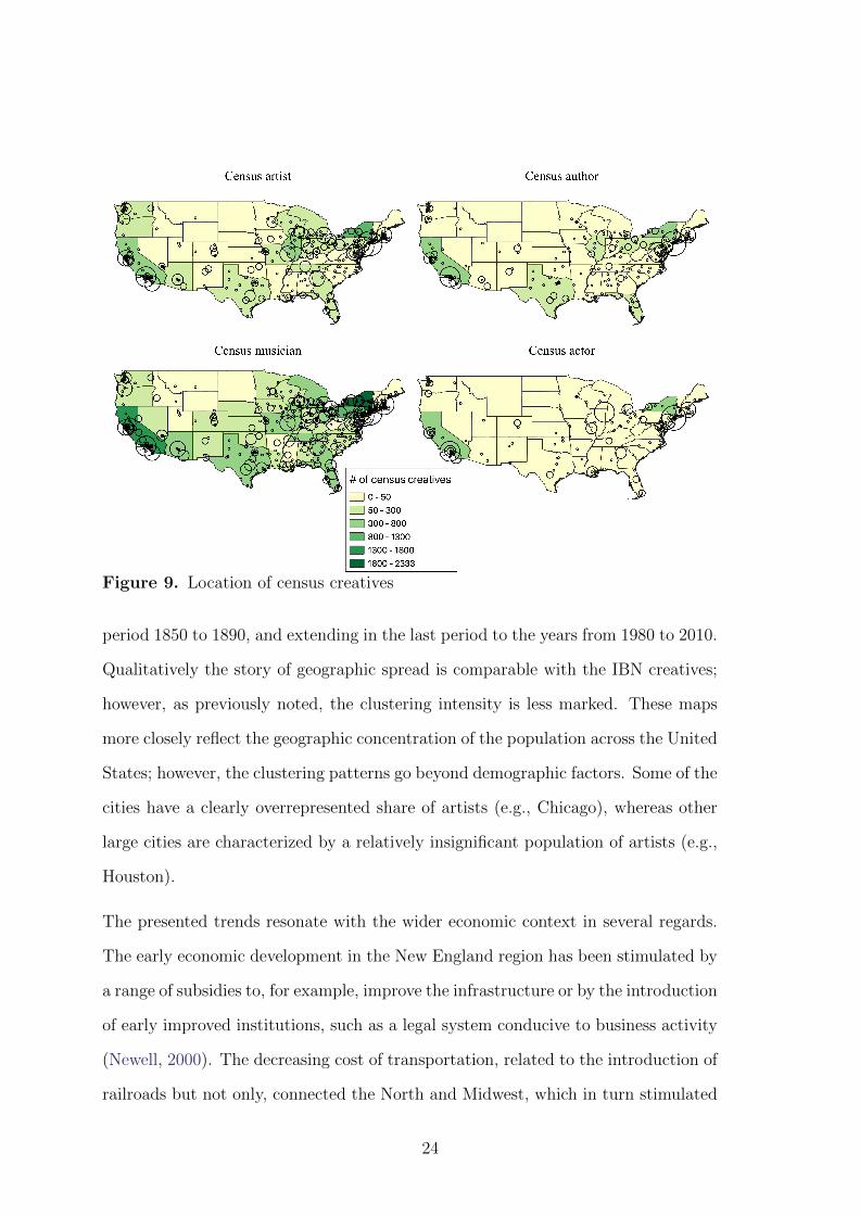
Figure 9. Location of census creatives

period 1850 to 1890, and extending in the last period to the years from 1980 to 2010.

Qualitatively the story of geographic spread is comparable with the IBN creatives;

however, as previously noted, the clustering intensity is less marked. These maps

more closely reflect the geographic concentration of the population across the United

States; however, the clustering patterns go beyond demographic factors. Some of the

cities have a clearly overrepresented share of artists (e.g., Chicago), whereas other

large cities are characterized by a relatively insignificant population of artists (e.g.,

Houston).

The presented trends resonate with the wider economic context in several regards.

The early economic development in the New England region has been stimulated by

a range of subsidies to, for example, improve the infrastructure or by the introduction

of early improved institutions, such as a legal system conducive to business activity

(Newell, 2000). The decreasing cost of transportation, related to the introduction of

railroads but not only, connected the North and Midwest, which in turn stimulated

24

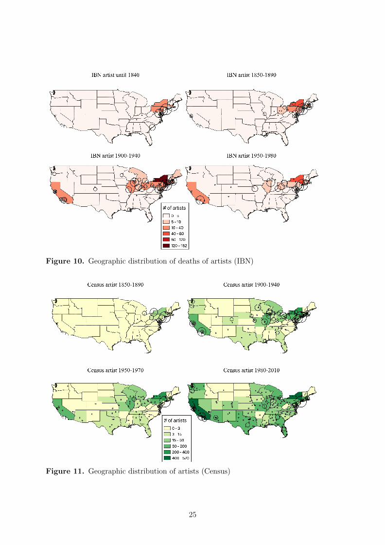
Figure 10. Geographic distribution of deaths of artists (IBN)

Figure 11. Geographic distribution of artists (Census)

25

not only migration, but also economic growth (Fogel, 1965). The rapid expansion

of settlements to the West opened up vast frontier lands, which became connected

by rail already in 1869, and with the advent of the automobile decreased further

the travel cost. Improved connectivity and the resulting high inflow of workers

contributed to the spread of people, goods, and also ideas.

Figure 12 depicts the clustering patterns of actors, which are particularly fascinating.

The deaths of all famous IBN actors before 1840 occurred in New York City, later

also in other cities of the Mid West, and eventually on the West Coast, quite as for

artists. However, the period after 1950 shows a remarkable concentration in just

two cities: New York and Los Angeles. The dominance of Los Angeles is related to

the rapid growth of Hollywood and is in line with other economic history accounts

of the development and dominance of the US movie industry (e.g., Bakker, 2005;

Sedgwick and Pokorny, 2010).7 The forces that have created this geographic cluster

include California’s natural advantages (Ellison and Glaeser, 1997) in the form of

sunlight, climate and the variety of landscape, which are particularly important for

film-making. Similar results emerge if one looks at the more numerous observations

from the census data in Figure 13: The states of New York and California remarkable

dominate the landscape.

Measuring the geographic concentration of creatives

In an attempt to introduce a measure of the extent of geographic concentration,

we compile Gini concentration indices for each of the creative occupations since

1850. The series are shown in Figure 14, along with the Gini concentration index

for teachers to provide some context. As one would expect, teachers are the most

evenly distributed group of workers. The Gini index for teachers is almost constant

and below 0.1 since the 1960s, which is the result of overall access to education

7Changes over time in clustering patterns for IBN and census musicians are depicted in AppendixFigures A6 and A7, and for authors in Figures A8 and A9.

26

Figure 12. Geographic distribution of deaths of actors (IBN)

Figure 13. Geographic distribution of actors (Census)

27

(Goldin and Katz, 2010). At the other extreme are actors, who exhibit the greatest

concentration. This is in line with the previously observed and discussed extraor-

dinary clustering of actors (see Figure 9). Authors and artists exhibit a very high

concentration in the earliest decades, which is followed by a gradual decrease in

concentration from about the 1940s. The Gini coefficient for authors and artists

converges at the value of about 0.6. The patterns and extent of concentration seem

very similar for authors and artists, which is likely a result of analogies in how

the two groups produce and disseminate their output: the production can occur

remotely, whether writing a book or painting, but both require important access

to supply-related infrastructure (publishers or gallerists and art museums). More-

over, the spillovers from interaction with other creatives are typically centered in

specialized locations (e.g., Borowiecki, 2013). In some contrast to this, musicians

concentrate less than artists and authors, albeit much higher than teachers. This

could be due to the necessity to locate close to one audiences, especially consider-

ing live performances, but also appearances on the radio, which were initially more

localized.

It is also interesting to observe the long-term decreases in the concentration of artists,

authors and musicians over the course of the second half of the 20th century. These

trends relate possibly to the various improvements in the transport infrastructure

and communication technologies, which have decentred some of the creative activity

away from artistic clusters towards the individual consumers (Borowiecki et al.,

2016).

Interdependencies across creative clusters

The data allows us also to explore cluster interdependencies and how cluster sizes

of various domains relate to each other. These relationships are shown for census

creatives in Table 3, using OLS-models (uneven columns) and Poisson-models (even

28

0.2

.4.6

.81

Gin

i con

cent

ratio

n in

dex

1850 1900 1950 2000Census year

Artist MusicianAuthor ActorTeacher

Figure 14. Gini concentration index across creative occupations

columns). The regressions now include year fixed effects to account for unobservable

differences across time. To account for differences in city size, all models include

further controls for the logged population of a city. Since two of the creative occu-

pations include teachers (i.e., artists and musicians), we further include controls for

the number of teachers, as recorded by the census.8

The correlations are positive and typically estimated with high statistical precision.

For example, in column (1) we can observe that a one percent increase in the num-

ber of authors is associated with a 0.33% increase in the population of artists. The

relationships are in general in the range between 0.06% and 0.33%, and also quali-

tatively consistent when estimated with Poisson-models. The overwhelming insight

is that creatives mix: cities that are the domicile for a certain type of creatives (e.g.,

visual artists) are typically also more popular among individuals from other creative

domains (e.g., authors or musicians).

8The results would remain qualitatively the same, if the teacher control variable was not in-cluded. Appendix Table A3 estimates how creative clusters interrelate for case of famous IBNcreatives.

29

Dependent variable:

log(Artist) Artist log(Author) Author log(Musician) MusicianOLS Poisson OLS Poisson OLS Poisson

(1) (2) (3) (4) (5) (6)

log(author) 0.33∗∗∗ 9.90∗∗∗ 0.13∗∗∗ 24.68∗∗∗

(0.03) (1.49) (0.02) (2.89)log(artist) 0.21∗∗∗ 11.47∗∗∗ 0.23∗∗∗ 31.22∗∗∗

(0.02) (2.55) (0.02) (3.22)log(actor) 0.21∗∗∗ 2.56∗∗ 0.24∗∗∗ 1.48 0.19∗∗∗ 10.09∗∗∗

(0.04) (1.21) (0.04) (1.79) (0.03) (3.21)log(musician) 0.17∗∗∗ 15.49∗∗∗ 0.06∗∗∗ 25.55∗∗∗

(0.02) (2.82) (0.01) (9.59)log(teacher) 0.09∗∗∗ 24.43∗∗∗ 0.02∗∗∗ 13.01 0.16∗∗∗ 115.58∗∗∗

(0.01) (3.98) (0.01) (9.05) (0.02) (9.17)log(city population) 0.16∗∗∗ 58.69∗∗∗ 0.02∗ 16.91∗ 0.34∗∗∗ 101.22∗∗∗

(0.02) (5.46) (0.01) (9.04) (0.03) (13.50)

Year FE? Yes Yes Yes Yes Yes Yes

Observations 3,506 3,506 3,506 3,506 3,506 3,506R2 0.54 0.51 0.63Adjusted R2 0.54 0.50 0.62Log Likelihood −110,523.70 −77,481.23 −185,492.60Akaike Inf. Crit. 221,085.30 155,000.50 371,023.20Residual Std. Error (df = 3487) 1.46 1.16 1.70F Statistic (df = 18; 3487) 228.88∗∗∗ 198.02∗∗∗ 323.31∗∗∗

Note: ∗p<0.1; ∗∗p<0.05; ∗∗∗p<0.01

Table 3. Interrelation of clusters across artistic domains

The role of famous artists

Finally, we investigate the interplay between famous and average creatives. Here we

explore the probability of a census respondent reporting a creative occupation and

how this relates to the presence of famous creatives in the same city in the past.

The estimated model is basically the same as reported previously in Equation 1,

but now in addition accounts for the history of significant artistic activity, measured

as the number of deaths of famous IBN creatives that occurred in the decade prior

to the given census. The identification of deaths measured at residence of census

respondent during ten years prior to the given census enables a certain time lag for

the person inspired by a famous IBN creative to become a creative herself.

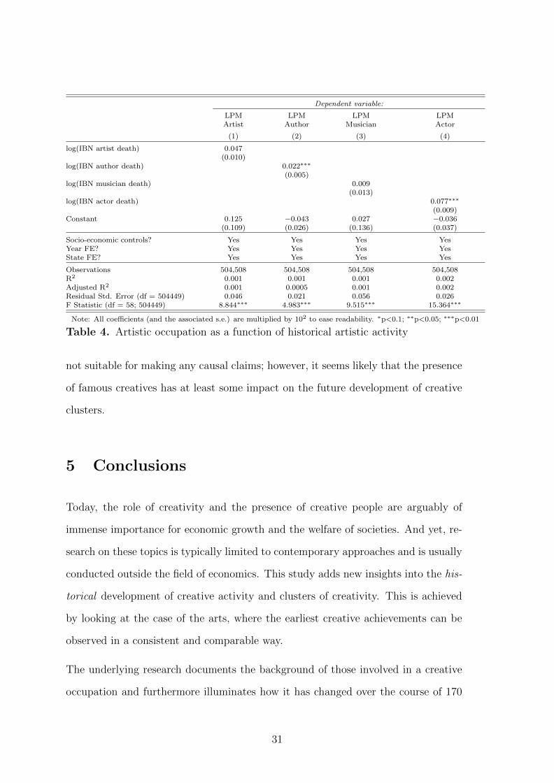
The results are summarized in Table 4 and imply that places with greater artistic

activity (i.e., where more creatives within a domain have died) tend to have more

people involved in creative occupations within the same domain, albeit the results

are statistically significant only for the case of authors and actors. This model is

30

Dependent variable:


(1) (2) (3) (4)

log(IBN artist death) 0.047(0.010)

log(IBN author death) 0.022∗∗∗

(0.005)log(IBN musician death) 0.009

(0.013)log(IBN actor death) 0.077∗∗∗

(0.009)Constant 0.125 −0.043 0.027 −0.036

(0.109) (0.026) (0.136) (0.037)

Socio-economic controls? Yes Yes Yes YesYear FE? Yes Yes Yes YesState FE? Yes Yes Yes Yes

Observations 504,508 504,508 504,508 504,508R2 0.001 0.001 0.001 0.002Adjusted R2 0.001 0.0005 0.001 0.002Residual Std. Error (df = 504449) 0.046 0.021 0.056 0.026F Statistic (df = 58; 504449) 8.844∗∗∗ 4.983∗∗∗ 9.515∗∗∗ 15.364∗∗∗


Table 4. Artistic occupation as a function of historical artistic activity

not suitable for making any causal claims; however, it seems likely that the presence

of famous creatives has at least some impact on the future development of creative

clusters.

5 Conclusions

Today, the role of creativity and the presence of creative people are arguably of

immense importance for economic growth and the welfare of societies. And yet, re-

search on these topics is typically limited to contemporary approaches and is usually

conducted outside the field of economics. This study adds new insights into the his-

torical development of creative activity and clusters of creativity. This is achieved

by looking at the case of the arts, where the earliest creative achievements can be

observed in a consistent and comparable way.

The underlying research documents the background of those involved in a creative

occupation and furthermore illuminates how it has changed over the course of 170

31

years. Some of the disclosed patterns echo the overall socio-demographic trends

of the period covered, but there are several novel and interesting insights: The

proportion of female creatives is relatively high, time constraints can be a hindrance

for taking up a creative occupation, racial inequality is present and tends to change

only slowly, and access to financial resources within a family facilitates the uptake

of an artistic occupation.

Furthermore, we shed light on the geography of creative clusters in the United

States and explain how these have evolved over time and across various domains.

Even though it may seem that some of the patterns are already known — for ex-

ample, that New York City is a very significant center for the arts — the extent of

the dominance has not yet been quantified before, nor has it been compared across

creative domains. Finally, by linking the census records with data on famous IBN

creatives, the role of famous individuals for the growth of local clusters and creative

employment is explored. Famous creatives have some influence on people taking

up creative occupations and are related to the size of creative centers. Typically,

superstar economies (Rosen, 1981) are criticized by the public mainly due to the

extreme earnings received by a small group of individuals at the very top of the

income scale. The insights presented here suggest the possibility of a positive ex-

ternality of superstars in the form of a potentially long-lasting heritage that some

famous creatives leave behind.

This research gives rise to several new questions. In particular, the question of how

the presence of a famous creative impacts others: Does she introduce new knowledge,

practices, networks, or infrastructure, or a multiple of these factors, which then

potentially persist over time? Or is it perhaps the case that her presence stimulates

the demand within a creative domain due to factors related to local identity and

heritage (for a related discussion, see Borowiecki, 2015b)?

Of interest for contemporary policy makers and the public is also whether and how

32

the historical development of creative activity is nowadays related to creativity.

Anecdotally, there seems to be a very high overlap between the creative clusters

historically and the startup landscape in the United States these days. We have

motivated this research by disclosing a strong and long-term correlation between

artistic activity and entrepreneurial outcomes. According to Compass (2015), six

US cities are listed among the global top-10 startup ecosystems, and the list begins

with San Francisco (Silicon Valley), New York City, Los Angeles and Boston; that

is, cities that have been identified in the underlying research as significant creative

clusters in history. These cities are obviously also centers of higher education with

some of the top universities in the country. Certainly the role of education cannot

be overlooked, as it is likely at least as important as artistic activity in explaining

why these areas are and have been centers of entrepreneurial outcomes (for a more

detailed discussion see Goldin and Katz, 2010). However, while it is beyond the

scope of this study to contribute to the debate on how artistic creativity is related to

startup activity, it becomes clear that these concepts are related and very persistent

over time, perhaps even more so than previously thought.

33

References

Alper, Neil O. and Gregory H. Wassal, “Artists’ Labor Market Experiences:

A Preliminary Analysis Using Longitudinal Data,” in M. Heikkinen and T. Koshi-

nen, eds., Economics of Artists and Arts Policy: A Selection of Papers, Helsinki:

The Arts Council of Finland, 1998.

and , “Artists’ Careers and Their Labor Markets,” in V. Ginsburgh and

D. Throsby, eds., Handbook of the Economics of Art and Culture, Amsterdam:

Elsevier, 2006.

Andersen, “Location and spatial clustering of artists,” Regional Science and Urban

Economics, 2014, 47, 128 – 137.

Ateca-Amestoy, Victoria, “Determining heterogeneous behavior for theater at-

tendance,” Journal of Cultural Economics, 2008, 32 (2), 127–151.

Ateca-Amestoy, Victoria Maria, Victor Ginsburgh, Isidoro Mazza, John

O’Hagan, and Juan Prieto-Rodriguez, Enhancing Participation in the Arts

in the EU, Mannheim: Springer, 2017.

Bakker, Gerben, “The decline and fall of the European film industry: sunk costs,

market size, and market structure, 1890–1927,” Economic History Review, 2005,

58 (2), 310–351.

Benhamou, Francoise, “Artist’s labour markets,” in Ruth Towse, ed., A Handbook

of Cultural Economics, Cheltenham: Edward Elgar Publishing, 2011, chapter 7,

pp. 53–58.

Blanchflower, David G. and Andrew J. Oswald, “What Makes an En-

trepreneur?,” Journal of Labor Economics, 1998, 16 (1), 26–60.

Borowiecki, Karol Jan, “Geographic clustering and productivity: An instrumen-

tal variable approach for classical composers,” Journal of Urban Economics, 2013,

34

73 (1), 94–110.

, “Agglomeration Economies in Classical Music,” Papers in Regional Science,

2015a, 94 (3), 443–68.

, “Historical origins of cultural supply in Italy,” Oxford Economic Papers, 2015b,

67 (3), 781–805.

, “How Are You, My Dearest Mozart? Well-being and Creativity of Three Famous

Composers Based on their Letters,” Review of Economics and Statistics, 2017, 99

(4), 591–605.

and John W. O’Hagan, “Historical Patterns Based on Automatically Ex-

tracted Data: The Case of Classical Composers,” Historical Social Research (Sec-

tion ‘Cliometrics’), 2012, 37 (2), 298–314.

and Kathryn Graddy, “Immigrant Artists: Enrichment or Displacement?,”

CEPR Discussion Papers 13070, C.E.P.R. Discussion Papers July 2018.

, Neil Forbes, and Antonella Fresa, Cultural Heritage in a Changing World,

Springer, 2016.

Burger-Helmchen, Thierry, The Economics of Creativity: Ideas, Firms and Mar-

kets, London: Routledge, 2013.

Compass, “The Global Startup Ecosystem Ranking 2015,” The Startup Ecosystem

Report Series, 2015.

Crafts, Nicholas, British Economic Growth during the Industrial Revolution, Ox-

ford: Clarendon Press, 1985.

de la Croix, David and Omar Licandro, “The longevity of famous people from

Hammurabi to Einstein,” Journal of Economic Growth, 2015, 20 (3), 263–303.

35

Duranton, Gilles and Henry G. Overman, “Testing for Localization Using

Micro-Geographic Data,” The Review of Economic Studies, 2005, 72 (4), 1077–

1106.

Ellison, Glenn and Edward L. Glaeser, “Geographic Concentration in U.S.

Manufacturing Industries: A Dartboard Approach,” Journal of Political Economy,

1997, 105 (5), 889–927.

and , “The Geographic Concentration of Industry: Does Natural Advantage

Explain Agglomeration?,” American Economic Review, May 1999, 89 (2), 311–

316.

Etro, Federico and Laura Pagani, “The Market for Paintings in Italy During

the Seventeenth Century,” Journal of Economic History, 2012, 72, 423–447.

Fairlie, Robert W., Arnobio Morelix, E.J. Reedy, and Joshua Russell, The

Kauffman Index 2015: Startup Activity. National Trends, Kansas City: Kauffman

Foundation, 2015.

Falck, Oliver, Michael Fritsch, Stephan Heblich, and Anne Otto, “Music in

the Air: Estimating the Social Return to Cultural Amenities,” Journal of Cultural

Economics, 2018, 42, 365–391.

Florida, Richard, The rise of the creative class: And how it’s transforming work,

leisure, community, and everyday life, New York: Basic Books, 2002.

Fogel, Robert William, Railroads and American Economic Growth: Essays in

Economic History, Baltimore: Johns Hopkin Press, 1965.

Fujita, Masahisa, Paul R. Krugman, and Anthony Venables, The Spatial

Economy: Cities, Regions, and International Trade, Boston: MIT Press, 1999.

Galenson, David W., Old Masters and Young Geniuses: The Two Life Cycles of

Artistic Creativity, Princeton: Princeton University Press, 2007.

36

and Bruce A. Weinberg, “Age and the Quality of Work: The Case of Modern

American Painters,” Journal of Political Economy, August 2000, 108 (4), 761–777.

and , “Creating Modern Art: The Changing Careers of Painters in France from

Impressionism to Cubism,” American Economic Review, 2001, 91 (4), 1063–1071.

Gergaud, Olivier, Morgane Laouenan, and Etienne Wasmer, “A Brief His-

tory of Human Time: Exploring a database of ’notable people’,” Sciences Po

Economics Discussion Papers No 2016-03, 2016.

Gibson, Campbell and Kay Jung, “Historical Census Statistics On Population

Totals By Race, 1790 to 1990, and By Hispanic Origin, 1970 to 1990, For Large

Cities And Other Urban Places In The United States,” U.S. Census Bureau Pop-

ulation Division Working Paper No. 76, 2005.

Glaeser, Edward L., “Cities, Information and Economic Growth,” Cityscape,

1994, 1 (1), 9–47.

, “The New Economics of Urban and Regional Growth,” in M. Feldman G. Clark

and M. Gertler, eds., The Oxford Handbook of Economic Geography, Oxford: Ox-

ford University Press, 2003, pp. 83–98.

, “Book Review of Richard Florida’s ”The Rise of the Creative Class”,” 2004.

, Jed Kolko, and Albert Saiz, “Consumer city,” Journal of Economic Geog-

raphy, 2001, 1 (1), 27–50.

, Stuart S. Rosenthal, and William C. Strange, “Urban economics and

entrepreneurship,” Journal of Urban Economics, 2010, 67 (1), 1 – 14.

Goldin, Claudia, “The Quiet Revolution That Transformed Women’s Employ-

ment, Education, and Family,” American Economic Review, 2006, 96 (2), 1–21.

and Lawrence F. Katz, The Race between Education and Technology, Boston:

Harvard University Press, 2010.

37

Graddy, Kathryn, “Taste Endures! The Rankings of Roger de Piles and Three

Centures of Art Prices,” Journal of Economic History, 2013, 73, 765–790.

Grove Music Online, Oxford Music Online, Oxford University Press, 2013.

Heilbrun, James and Charles M. Gray, The Economics of Art and Culture,

Cambridge University Press, 2001.

Hellmanzik, Christiane, “Location matters: Estimating cluster premiums for

prominent modern artists,” European Economic Review, February 2010, 54 (2),

199–218.

IPUMS, “Integrated Public Use Microdata Series,” https://usa.ipums.org/

2015. Accessed: Spring 2015.

, “Integrated Occupation and Industry Codes and Occupational Standing Vari-

ables in the IPUMS,” https://usa.ipums.org/usa/chapter4/chapter4.shtml

2017. Accessed: 2017-04-18.

Jovanovich, Monica E. and Melissa Renn, Corporate Patronage of Art and

Architecture in the United States, Late 19th Century to the Present, Bloomsbury:

Bloomsbury Visual Arts, 2019.

Knudsen, Brian, Richard Florida, Kevin Stolarick, and Gary Gates, “Den-

sity and Creativity in U.S. Regions,” Annals of the Association of American Ge-

ographers, 2008, 98 (2), 461–478.

Lovell, Margaretta M., Art in a Season of Revolution: Painters, Artisans, and

Patrons in Early America, Philadelphia: University of Pennsylvania Press, 2007.

Ludwig, Arnold M., The Price of Greatness: Resolving the Creativity and Mad-

ness Controversy, New York: The Guilford Press, 1995.

Maloney, William F. and Felipe Valencia Caicedo, “Engineers, Innovative

Capacity and Development in the Americas,” IZA Discussion Paper No. 8271,

38

https://usa.ipums.org/

https://usa.ipums.org/usa/chapter4/chapter4.shtml

2014.

Menger, Pierre-Michel, The Economics of Creativity: Art and Achievement un-

der Uncertainty, Boston: Harvard University Press, 2014.

Mitchell, Sara, “London Calling? Agglomeration Economies in Literature since

1700,” Journal of Urban Economics, 2019, 112, 16–32.

Newell, Margaret Alan, “The Birth of New England in the Atlantic Economy:

From its Beginning to 1770,” in Peter Temin, ed., Engines of Enterprise: An Eco-

nomic History of New England, Boston: Harvard University Press, 2000, p. 11–68.

OECD, Resilient Economies for Inclusive Societies, Paris: OECD, 2014.

O’Hagan, John W. and Christiane Hellmanzik, “Clustering and Migration

of Important Visual Artist: Broad Historical Evidence,” Historical Methods: A

Journal of Quantitative and Interdisciplinary History, 2008, 40 (3), 121–36.

and Karol Jan Borowiecki, “Birth Location, Migration and Clustering of

Important Composers: Historical Patterns,” Historical Methods: A Journal of

Quantitative and Interdisciplinary History, 2010, 43 (2), 81–91.

O’Hagan, John and Karol Jan Borowiecki, “Birth Location, Migration, and

Clustering of Important Composers,” Historical Methods: A Journal of Quanti-

tative and Interdisciplinary History, 2010, 43 (2), 81–90.

Puga, Diego, “The magnitude and causes of agglomeration economies,” Journal

of Regional Science, 2010, 50 (1), 203–219.

Rosen, Sherwin, “The Economics of Superstars,” American Economic Review,

1981, 71 (5), 845–858.

Rosenthal, S. and W. Strange, “Evidence on the Nature and Sources of Ag-

glomeration Economies,” in J.V. Henderson and J.F. Thisse, eds., Handbook of

Regional and Urban Economics, Amsterdam: Elsevier, 2004.

39

Sedgwick, John and Michael Pokorny, “Profitability trends in Hollywood, 1929

to 1999: Somebody must know something,” Economic History Review, 2010, 63

(1), 56–84.

Tao, “Agglomeration economies in creative industries,” Regional Science and Urban

Economics, 2019, 77, 141 – 154.

Throsby, David, Economics and Culture, Cambridge: Cambridge University Press,

2001.

Towse, Ruth, “Creativity, Copyright and the Creative Industries Paradigm,” Kyk-

los, 2010, 63 (3).

UNCTAD, Creative Economy: A Feasible Development Option, Geneva: UNC-

TAD, 2010.

, Creative Economy Outlook: Trends in international trade in creative industries,

Geneva: UNCTAD, 2018.

Weber, Clint B., The Treasured Collection of Golden Heart Farm: A Biography of

Wilhelmina Weber Furlong, New York: The Weber Furlong Publishing Company,

2012.

40

Online Appendix

A Additional robustness tests

The novel long-term approach pursued in the underlying paper comes at a cost– the measurement of some of the variables has (usually slightly) changed acrossthe 16 decades covered, while other variables are available only over limited timeperiods.

It is important to note that that the changes across the Census waves in the definitionor measurement of some of the variables covered, have been made quite certainlyindependently from changes in the labor market of creatives. Furthermore, thechanges go sometimes in either direction (for example, we observe both, increasesand decreases in the cut-off point of age). Therefore, while the census changes maystill lead to biased estimates, these biases – given the long time-period covered –should not be very meaningful on average. Nonetheless, a series of robustness testshas been conducted to check on the consistency of the models estimated.

One particular change in the cut-off of a variable concerns the occupation variable(occ1950 ), which has been obtained in the earliest two census waves covered indi-viduals aged 15+, but in later editions also respondents aged 14+ and 16+ havebeen surveyed. The volatility of the cut-off point regarding age is rather small, andconcerns primarily individuals who – in many cases - have not reached yet the ageto become involved in a creative occupation (or perhaps even in most occupations).Nonetheless, in an attempt to check on this potential bias, one may want to dropall individuals below the age of 16 to ensure that the same age cohort is coveredthroughout the time period. This has been done and the results are indistinguishablefrom the baseline specification, which is encouraging.

41

B Additional Tables and Figures

B.1 Socio-economic background of creatives: Additional mod-els

Dependent variable:


(1) (2) (3) (4)

female −0.0001 0.022∗∗∗ 0.233∗∗∗ −0.010∗∗∗

(0.006) (0.006) (0.012) (0.003)age 0.007∗∗∗ 0.007∗∗∗ 0.011∗∗∗ 0.0005∗

(0.001) (0.001) (0.001) (0.0003)age2 −0.0001∗∗∗ −0.0001∗∗∗ −0.0001∗∗∗ −0.00001∗∗

(0.00001) (0.00001) (0.00001) (0.00000)married −0.081∗∗∗ −0.073∗∗∗ −0.122∗∗∗ −0.029∗∗∗

(0.009) (0.008) (0.016) (0.004)separated −0.081∗∗∗ −0.066∗∗∗ −0.163∗∗∗ −0.027∗∗∗

(0.013) (0.011) (0.025) (0.005)divorced −0.055∗∗∗ −0.075∗∗∗ −0.097∗∗∗ −0.018∗∗∗

(0.010) (0.009) (0.019) (0.004)widowed −0.108∗∗∗ −0.102∗∗∗ −0.262∗∗∗ −0.026∗∗∗

(0.009) (0.008) (0.018) (0.004)family size −0.017∗∗∗ −0.011∗∗∗ −0.028∗∗∗ −0.006∗∗∗

(0.002) (0.002) (0.005) (0.001)number children −0.004 0.003 −0.017∗∗∗ 0.001

(0.003) (0.002) (0.006) (0.001)black −0.105∗∗∗ −0.062∗∗∗ −0.023∗ −0.005∗∗

(0.004) (0.004) (0.012) (0.002)native 0.047 −0.035 0.069 −0.011

(0.038) (0.022) (0.064) (0.010)asian −0.032∗∗ −0.112∗∗∗ −0.247∗∗∗ −0.039∗∗∗

(0.014) (0.010) (0.024) (0.004)other −0.042∗∗∗ −0.060∗∗∗ −0.030 −0.021∗∗∗

(0.011) (0.007) (0.022) (0.005)mixed 0.002 −0.011 0.067 0.058∗∗∗

(0.025) (0.023) (0.052) (0.020)earnings −0.009∗∗∗ −0.005∗∗∗ 0.007∗∗∗ −0.0005∗

(0.001) (0.001) (0.001) (0.0002)family income 0.009∗∗∗ 0.008∗∗∗ −0.007∗∗ −0.0005

(0.001) (0.002) (0.003) (0.001)education 0.026∗∗∗ 0.032∗∗∗ 0.123∗∗∗ 0.003∗∗∗

(0.001) (0.001) (0.002) (0.0003)Constant −0.139∗∗∗ −0.246∗∗∗ −0.304∗∗∗ 0.032∗∗∗

(0.022) (0.018) (0.044) (0.008)




Table A1. Socio-economic background of creatives: Education and income

42

Dependent variable:


(1) (2) (3) (4)

female −0.038∗∗∗ −0.003 0.047∗∗ −0.022∗∗∗

(0.012) (0.011) (0.021) (0.006)age 0.007∗∗∗ 0.010∗∗∗ 0.018∗∗∗ −0.0002

(0.001) (0.001) (0.002) (0.001)age2 −0.0001∗∗∗ −0.0001∗∗∗ −0.0002∗∗∗ −0.00001

(0.00001) (0.00001) (0.00002) (0.00001)married −0.146∗∗∗ −0.085∗∗∗ −0.240∗∗∗ −0.047∗∗∗

(0.016) (0.013) (0.026) (0.009)separated −0.155∗∗∗ −0.121∗∗∗ −0.287∗∗∗ −0.045∗∗∗

(0.024) (0.020) (0.045) (0.010)divorced −0.073∗∗∗ −0.086∗∗∗ −0.108∗∗∗ −0.004

(0.021) (0.017) (0.035) (0.011)widowed −0.163∗∗∗ −0.114∗∗∗ −0.365∗∗∗ −0.030∗∗∗

(0.017) (0.013) (0.028) (0.009)family size −0.023∗∗∗ −0.021∗∗∗ −0.044∗∗∗ −0.006∗∗∗

(0.004) (0.002) (0.006) (0.002)number children −0.009∗∗ 0.001 −0.022∗∗∗ −0.008∗∗∗

(0.004) (0.002) (0.007) (0.003)black −0.199∗∗∗ −0.150∗∗∗ −0.227∗∗∗ −0.030∗∗∗

(0.008) (0.007) (0.018) (0.005)native −0.094 −0.129∗∗∗ −0.060 −0.040

(0.066) (0.047) (0.138) (0.027)asian −0.078∗∗∗ −0.170∗∗∗ −0.386∗∗∗ −0.110∗∗∗

(0.027) (0.022) (0.040) (0.010)other −0.219∗∗∗ −0.270∗∗∗ −0.520∗∗∗ −0.105∗∗∗

(0.020) (0.013) (0.037) (0.009)mixed −0.048 −0.194∗∗∗ −0.074 0.094∗

(0.059) (0.044) (0.109) (0.056)migrant 0.039∗∗∗ 0.051∗∗∗ 0.131∗∗∗ 0.023∗∗∗

(0.008) (0.006) (0.013) (0.004)log(city population) 0.029∗∗∗ 0.019∗∗∗ 0.038∗∗∗ 0.023∗∗∗

(0.002) (0.002) (0.004) (0.002)Constant −0.089 −0.366∗∗∗ −0.138 −0.093∗∗∗

(0.121) (0.062) (0.215) (0.018)




Table A2. Socio-economic background of creatives: City size and migrants

43

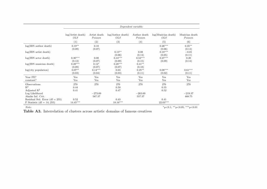
Dependent variable:

log(Artist death) Artist death log(Author death) Author death log(Musician death) Musician deathOLS Poisson OLS Poisson OLS Poisson

(1) (2) (3) (4) (5) (6)

log(IBN author death) 0.19∗∗ 0.10 0.26∗∗∗ 0.35∗∗

(0.09) (0.07) (0.06) (0.14)log(IBN artist death) 0.13∗∗ 0.08 0.18∗∗∗ −0.01

(0.06) (0.14) (0.05) (0.11)log(IBN actor death) 0.30∗∗∗ 0.08 0.44∗∗∗ 0.52∗∗∗ 0.27∗∗∗ 0.20

(0.12) (0.07) (0.09) (0.15) (0.09) (0.14)log(IBN musician death) 0.28∗∗∗ 0.12∗ 0.28∗∗∗ 0.41∗∗

(0.09) (0.07) (0.07) (0.18)log(city population) 0.07∗∗ 0.14∗∗∗ 0.03 0.25∗∗ 0.08∗∗∗ 0.61∗∗∗

(0.03) (0.04) (0.03) (0.11) (0.02) (0.11)

Year FE? Yes Yes Yes Yes Yes Yesconstant? Yes Yes Yes Yes Yes Yes

Observations 270 270 270 270 270 270R2 0.44 0.50 0.55Adjusted R2 0.41 0.47 0.52Log Likelihood −273.69 −263.69 −219.37Akaike Inf. Crit. 567.37 557.37 468.75Residual Std. Error (df = 255) 0.52 0.43 0.41F Statistic (df = 14; 255) 14.45∗∗∗ 18.16∗∗∗ 22.03∗∗∗

Note: ∗p<0.1; ∗∗p<0.05; ∗∗∗p<0.01

Table A3. Interrelation of clusters across artistic domains of famous creatives

02

46

8C

reat

ives

per

100

0 po

pula

tion

1850 1900 1950 2000Census year

Artist MusicianAuthor Actor

Figure A1. Share of household heads with artistic occupations

050

100

150

Dea

ths

of fa

mou

s cr

eativ

es

1800 1850 1900 1950Decade

Artist MusicianAuthor Actor

Figure A2. Deaths of famous creatives (IBN) by occupation

45

12

34

5F

amily

siz

e by

occ

upat

ion

1850 1900 1950 2000Census year


Figure A3. Family size by occupationNote: See Figure 2

46

Figure A4. Socio-economic background of creativesNote: This figure shows the point estimates (dots) and 95 per cent confidence bands based on robust s.e. (intervals) for the models presented in Table 1.

47

Figure A5. Socio-economic background of creatives by domainNote: This figure shows the point estimates (dots) and 95 per cent confidence bands based on robust s.e. (intervals) for the models presented in Table 2.

48

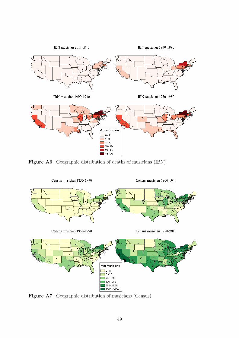
Figure A6. Geographic distribution of deaths of musicians (IBN)

Figure A7. Geographic distribution of musicians (Census)

49

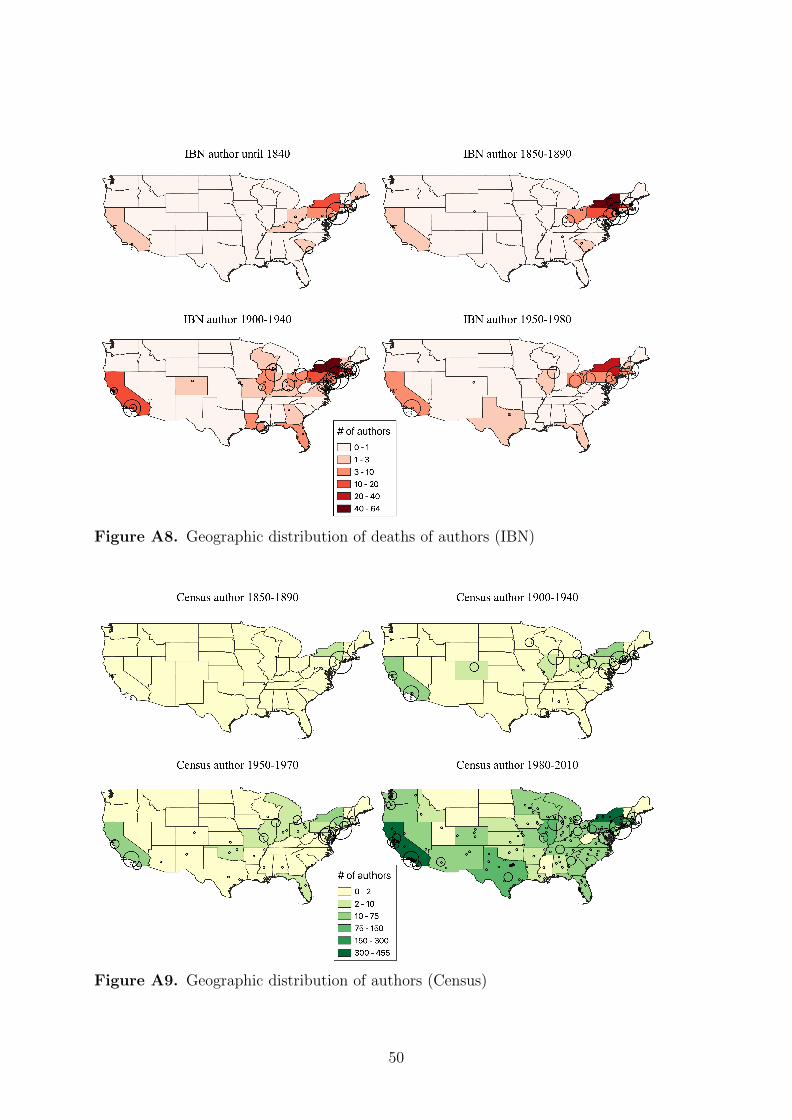
Figure A8. Geographic distribution of deaths of authors (IBN)

Figure A9. Geographic distribution of authors (Census)

50

Documents

What makes an artist? The evolution and clustering of