What is Quantum Thermodynamics?

Gian Paolo BerettaUniversita di Brescia, via Branze 38, 25123 Brescia, Italy

What is the physical significance of entropy? What is the physical origin of irreversibility? Doentropy and irreversibility exist only for complex and macroscopic systems?

For everyday laboratory physics, the mathematical formalism of Statistical Mechanics (canonicaland grand-canonical, Boltzmann, Bose-Einstein and Fermi-Dirac distributions) allows a successfuldescription of the thermodynamic equilibrium properties of matter, including entropy values. How-ever, as already recognized by Schrodinger in 1936, Statistical Mechanics is impaired by conceptualambiguities and logical inconsistencies, both in its explanation of the meaning of entropy and in itsimplications on the concept of state of a system.

An alternative theory has been developed by Gyftopoulos, Hatsopoulos and the present authorto eliminate these stumbling conceptual blocks while maintaining the mathematical formalism ofordinary quantum theory, so successful in applications. To resolve both the problem of the meaningof entropy and that of the origin of irreversibility, we have built entropy and irreversibility into thelaws of microscopic physics. The result is a theory that has all the necessary features to combineMechanics and Thermodynamics uniting all the successful results of both theories, eliminating thelogical inconsistencies of Statistical Mechanics and the paradoxes on irreversibility, and providing anentirely new perspective on the microscopic origin of irreversibility, nonlinearity (therefore includingchaotic behavior) and maximal-entropy-generation non-equilibrium dynamics.

In this long introductory paper we discuss the background and formalism of Quantum Thermo-dynamics including its nonlinear equation of motion and the main general results regarding thenonequilibrium irreversible dynamics it entails. Our objective is to discuss and motivate the form ofthe generator of a nonlinear quantum dynamical group “designed” so as to accomplish a unificationof quantum mechanics (QM) and thermodynamics, the nonrelativistic theory that we call QuantumThermodynamics (QT). Its conceptual foundations differ from those of (von Neumann) quantumstatistical mechanics (QSM) and (Jaynes) quantum information theory (QIT), but for thermody-

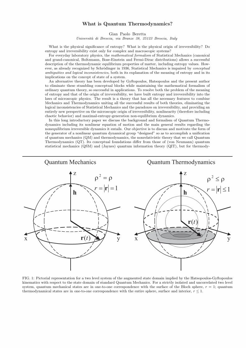
FIG. 1: Pictorial representation for a two level system of the augmented state domain implied by the Hatsopoulos-Gyftopouloskinematics with respect to the state domain of standard Quantum Mechanics. For a strictly isolated and uncorrelated two levelsystem, quantum mechanical states are in one-to-one correspondence with the surface of the Bloch sphere, r = 1; quantumthermodynamical states are in one-to-one correspondence with the entire sphere, surface and interior, r ≤ 1.

2

namic equilibrium (TE) states it reduces to the same mathematics, and for zero entropy states itreduces to standard unitary QM. By restricting the discussion to a strictly isolated system (non-interacting, disentangled and uncorrelated) we show how the theory departs from the conventionalQSM/QIT rationalization of the second law of thermodynamics.

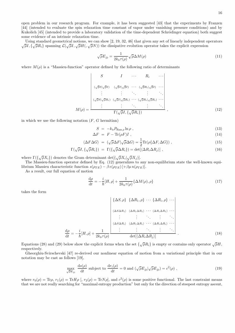
The nonlinear dynamical group of QT is construed so that the second law emerges as a theorem ofexistence and uniqueness of a stable equilibrium state for each set of mean values of the energy andthe number of constituents. To achieve this, QT assumes −kBTrρ ln ρ for the physical entropy andis designed to implement two fundamental ansatzs. The first is that in addition to the standard QMstates described by idempotent density operators (zero entropy), a strictly isolated system admitsalso states that must be described by non-idempotent density operators (nonzero entropy). Thesecond is that for such additional states the law of causal evolution is determined by the simultane-ous action of a Schroedinger-von Neumann-type Hamiltonian generator and a nonlinear dissipativegenerator which conserves the mean values of the energy and the number of constituents, and (in for-ward time) drives the density operator in the ’direction’ of steepest entropy ascent (maximal entropyincrease). The resulting positive nonlinear dynamical group (not just a semi-group) is well-definedfor all nonequilibrium states, no matter how far from TE. Existence and uniqueness of solutionsof the (Cauchy) initial state problem for all density operators, implies that the equation of motioncan be solved not only in forward time, to describe relaxation towards TE, but also backwards intime, to reconstruct the ’ancestral’ or primordial lowest entropy state or limit cycle from which thesystem originates.

I. INTRODUCTION

There is no dispute about the results, the mathematical formalism, and the practical consequences of the theories ofMechanics and Equilibrium Thermodynamics, even though their presentations and derivations still differ essentiallyfrom author to author in logical structure and emphasis. Both Mechanics (Classical and Quantum) and EquilibriumThermodynamics have been developed independently of one another for different applications, and have enjoyedinnumerable great successes. There are no doubts that the results of these theories will remain as milestones of thedevelopment of Science.

But as soon as they are confronted, Mechanics and Equilibrium Thermodynamics give rise to an apparent incom-patibility of results: a dilemma, a paradox that has concerned generations of scientists during the last century andstill remains unresolved. The problem arises when the general features of kinematics and dynamics in Mechanics areconfronted with the general features of kinematics and dynamics implied by Equilibrium Thermodynamics. Thesefeatures are in striking conflict in the two theories. The conflict concerns the notions of reversibility, availability ofenergy to adiabatic extraction, and existence of stable equilibrium states [1, 2]. Though perhaps presented with em-phasis on other related conflicting aspects, the apparent incompatibility of the theories of Mechanics and EquilibriumThermodynamics is universally recognized by all scientists that have tackled the problem [3]. What is not universallyrecognized is how to rationalize the unconfortable paradoxical situation [1].

The rationalization attempt better accepted within the physical community is offered by the theory of StatisticalMechanics. Like several other minor attempts of rationalization [1], Statistical Mechanics stems from the premise thatMechanics and Equilibrium Thermodynamics occupy different levels in the hierarchy of physical theories: they bothdescribe the same physical reality, but Mechanics (Quantum) is concerned with the true fundamental description,whereas Equilibrium Thermodynamics copes with the phenomenological description – in terms of a limited set ofstate variables – of systems with so many degrees of freedom that the fundamental quantum mechanical descriptionwould be overwhelmingly complicated and hardly reproducible.

When scrutinized in depth, this almost universally accepted premise and, therefore, the conceptual foundations ofStatistical Mechanics are found to be shaky and unsound. For example, they seem to require that we abandon theconcept of state of a system [4], a keystone of traditional physical thought. In spite of the lack of a sound conceptualframework, the mathematical formalism and the results of Statistical Mechanics have enjoyed such great successes thatthe power of its methods have deeply convinced almost the entire physical community that the conceptual problemscan be safely ignored.

The formalism of Statistical Mechanics has also provided mathematical tools to attempt the extension of theresults beyond the realm of thermodynamic equilibrium. In this area, the results have been successful in a varietyof specific nonequilibrium problems. The many attempts to synthetize and generalize the results have generatedimportant conclusions such as the Boltzmann equation, the Onsager reciprocity relations, the fluctuation- dissipationrelations, and the Master equations. But, again, the weakness of the conceptual foundations has forbidden so far thedevelopment of a sound unified theory of nonequilibrium.

The situation can be summarized as follows. On the one hand, the successes of Mechanics, Equilibrium Ther-modynamics, and the formalism of Statistical Mechanics for both equilibrium and nonequilibrium leave no doubts

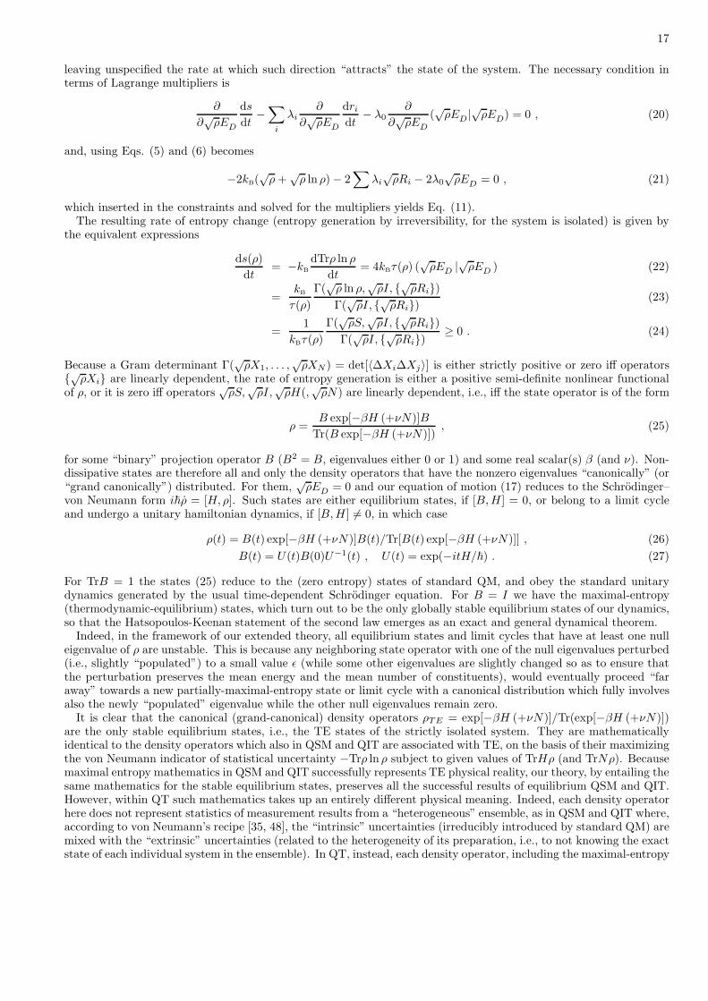
3

on the validity of their end results. On the other hand, the need remains of a coherent physical theory capable ofencompassing these same results within a sound unified unambiguous conceptual framework.

Of course, the vast majority of physicists would argue that there is no such need because there is no experimentalobservation that Statistical Mechanics cannot rationalize. But the problem at hand is not that there is a bodyof experimental evidence that cannot be regularized by current theories. Rather, it is that current theories havebeen developed and can be used only as ad-hoc working tools, successful to regularize the experimental evidence,but incapable to resolve conclusively the century-old fundamental questions on the physical roots of entropy andirreversibility, and on the general description of nonequilibrium. These fundamental questions have kept the scientificcommunity in a state of tension for longer than a century and cannot be safely ignored.

In short, the irreversibility paradox, the dilemma on the meaning of entropy, and the questions on the natureof nonequilibrium phenomena remain by and large unresolved problems. The resolution of each of these problemsrequires consideration of all of them at once, because they are all intimately interrelated.

The notion of stability of equilibrium has played and will play a central role in the efforts to fill the gap. Ofthe two main schools of thought that during the past few decades have attacked the problem, the Brussels schoolhas emphasized the role of instability and bifurcations in self-organization of chemical and biological systems, andthe Keenan school at MIT has emphasized that the essence of the second law of Thermodynamics is a statement ofexistence and uniqueness of the stable equilibrium states of a system.

The recognition of the central role that stability plays in Thermodynamics [5] is perhaps one of the most fundamentaldiscoveries of the physics of the last four decades, for it has provided the key to a coherent resolution of the entropy-irreversibility-nonequilibrium dilemma. In this article: first, we review the conceptual and mathematical frameworkof the problem; then, we discuss the role played by stability in guiding towards a coherent resolution; and, finally, wediscuss the resolution offered by the new theory – Quantum Thermodynamics – proposed by the Keenan school atMIT about twenty years ago (and, short of a definitive experimental proof or disproof, still only marginally recognizedby the orthodox physical community [6]).

Even though Quantum Thermodynamics is based on conceptual premises that are indeed quite revolutionary andentirely different from those of Statistical Mechanics, we emphasize the following:

• In terms of mathematical formalism, Quantum Thermodynamics differs from Statistical Mechanics mainly inthe equation of motion which is nonlinear, even though it reduces to the Schrodinger equation for all the statesof Quantum Mechanics, i.e., all zero-entropy states.

• In terms of physical meaning, instead, the differences are drastic. The significance of the state operator ofQuantum Thermodynamics is entirely different from that of the density operator of Statistical Mechanics, eventhough the two are mathematically equivalent, and not only because they obey different equations of motion.Quantum Thermodynamics postulates that the set of true quantum states of a system is much broader thanthe set contemplated in Quantum Mechanics.

• Conceptually, the augmented set of true quantum states is a revolutionary postulate with respect to traditionalquantum physics, although from the point of view of statistical mechanics practitioners, the new theory is notas traumatic as it seems.

• Paradoxically, the engineering thermodynamics community has already implicitly accepted the fact that entropy,exactly like energy, is a true physical property of matter and, therefore, the range of ’true states’ of a systemis much broader than that of Mechanics (zero entropy), for it must include the whole set of nonzero-entropystates.

• The new theory retains the whole mathematical formalism of Statistical Mechanics as regards thermodynamic(stable) equilibrium states – the formalism used by physics practitioners every day – but reinterprets it withina unified conceptual and mathematical structure in an entirely new way which resolves the open conceptualquestions on the nature of quantum states and on irreversibility paradox, and by proposing the steepest-entropy-ascent dynamical principle opens new vistas on the fundamental description of non-equilibrium states, offeringa powerful general equation for irreversible dynamics valid no matter how far from thermodynamic equilibrium.

II. THE COMMON BASIC CONCEPTUAL FRAMEWORK OF MECHANICS ANDTHERMODYNAMICS

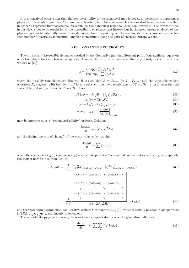
In this section, we establish the basic conceptual framework in which both Mechanics and Equilibrium Thermo-dynamics are embedded. To this end, we define the basic terms that are traditional keystones of the kinematic anddynamic description in all physical theories, and are essential in the discussion that follows. Specifically, we review the

4

concepts of constituent, system, property, state, equation of motion, process, reversibility, equilibrium, and stabilityof equilibrium [7].

The idea of a constituent of matter denotes a specific molecule, atom, ion, elementary particle, or field, that for agiven description is considered as indivisible. Within a given level of description, the constituents are the elementarybuilding blocks. Clearly, a specific molecule may be a constituent for the description of a certain class of phenomena,but not for other phenomena in which its internal structure may not be ignored and, therefore, a different level ofdescription must be chosen.

The kind of physical laws we are concerned with here are the most fundamental, i.e., those equally applicable atevery level of description, such as the great conservation principles of Mechanics.

A. Kinematics

A system is a (separable) collection of constituents defined by the following specifications: (a) the type and the rangeof values of the amount of each constituent; (b) the type and the range of values of each of the parameters which fullycharacterize the external forces exerted on the constituents by bodies other than the constituents, for example, theparameters that describe the geometrical shape of a container; and (c) the internal forces between constituents suchas the forces between molecules, the forces that promote or inhibit a chemical reaction, the partitions that separateconstituents in one region of space from constituents in another region, or the interconnections between separatedparts. Everything that is not included in the system is called the environment or the surroundings of the system.

At any instant in time, the values of the amounts of each type of constituent and the parameters of each externalforce do not suffice to characterize completely the condition of the system at that time. We need, in addition, thevalues of all the properties at the same instant in time. A property is an attribute that can be evaluated by meansof a set of measurements and operations which are performed on the system with reference to one instant in timeand result in a value – the value of the property – independent of the measuring devices, of other systems in theenvironment, and of other instants in time. For example, the instantaneous position of a particular constituent is aproperty.

Some properties in a given set are independent if the value of each such property can be varied without affectingthe value of any other property in the set. Other properties are not independent. For example, speed and kineticenergy of a molecule are not independent properties.

The values of the amounts of all the constituents, the values of all the parameters, and the values of a completeset of independent properties encompass all that can be said at an instant in time about a system and about theresults of any measurement or observation that may be performed on the system at that instant in time. As such, thecollection of all these values constitutes a complete characterization of the system at that instant in time: the stateof the system.

B. Dynamics

The state of a system may change with time either spontaneously due to its internal dynamics or as a result ofinteractions with other systems, or both. Systems that cannot induce any effects on each other’s state are calledisolated. Systems that are not isolated can influence each other in a number of different ways.

The relation that describes the evolution of the state of a system as a function of time is called the equation ofmotion.

In classical thermodynamics, the complete equation of motion is not known. For this reason, the description of achange of state is done in terms of the end states, i.e., the initial and the final states of the system, and the effectsof the interactions that are active during the change of state. Each mode of interaction is characterized by means ofwell-specified effects, such as the net exchanges of some additive properties across the boundaries of the interactingsystems. Even though the complete equation of motion is not known, we know that it must entail some importantconclusions traditionally stated as the laws of thermodynamics. These laws reflect some general and important facetsof the equation of motion such as the conditions that energy is conserved and entropy cannot be destroyed.

The end states and the effects of the interactions associated with a change of state of a system are said to specify aprocess. Processes may be classified on the basis of the modes of interaction they involve. For example, a process thatinvolves no influence from other systems is called a spontaneous process. Again, a process that involves interactionsresulting in no external effects other than the change in elevation of a weight (or an equivalent mechanical effect) iscalled a weight process.

Processes may also be classified on the basis of whether it is physically possible to annul all their effects. A process iseither reversible or irreversible. A process is reversible if there is a way to restore both the system and its environment

5

to their respective initial states, i.e., if all the effects of the process can be annulled. A process is irreversible if thereis no way to restore both the system and its environment to their respective initial states.

C. Types of states

Because the number of independent properties of a system is very large even for a system consisting of a singleparticle, and because most properties can vary over a large range of values, the number of possible states of a systemis very large. To facilitate the discussion, we classify the states of a system on the basis of their time evolution,i.e., according to the way they change as a function of time. We classify states into four types: unsteady, steady,nonequilibrium, and equilibrium. We further classify equilibrium states into three types: unstable, metastable, andstable.

Unsteady is a state that changes with time as a result of influences of other systems in its environment. Steady is astate that does not change with time despite the influences of other systems in the environment. Nonequilibrium is astate that changes spontaneously as a function of time, i.e., a state that evolves as time goes on even when the systemis isolated from its environment. Equilibrium is a state that does not change as a function of time if the system isisolated, i.e., a state that does not change spontaneously. Unstable equilibrium is an equilibrium state which, uponexperiencing a minute and short lived influence by a system in the environment, proceeds from then on spontaneouslyto a sequence of entirely different states. Metastable equilibrium is an equilibrium state that may be changed to anentirely different state without leaving net effects in the environment of the system, but this can be done only bymeans of interactions which have a finite temporary effect on the state of the environment. Stable equilibrium is anequilibrium state that can be altered to a different state only by interactions that leave net effects in the environmentof the system.

Starting either from a nonequilibrium or from an equilibrium state that is not stable, a system can be made tocause in its environment a change of state consisting solely in the raise of a weight. In contrast, if we start from astable equilibrium state such a raise of a weight is impossible. This impossibility is one of the consequences of thefirst law and the second law of thermodynamics [7].

III. THE BASIC MATHEMATICAL FRAMEWORK OF QUANTUM THEORY

The traditional structure of a physical theory is in terms of mathematical entities associated with each basic concept,and interrelations among such mathematical entities. In general, with the concept of system is associated a metricspace, and with the concept of state an element of a subset of the metric space called the state domain. The differentelements of the state domain represent all the different possible states of the system. With the concept of propertyis associated a real functional defined on the state domain. Different properties are represented by different realfunctionals, and the value of each property at a given state is given by the value of the corresponding functionalevaluated at the element in the state domain representing the state. Some of the functionals representing propertiesof the system may depend also on the amounts of constituents of the system and the parameters characterizing theexternal forces.

A. Quantum mechanics

In Quantum Mechanics, the metric space is a Hilbert space H (dimH ≤ ∞), the states are the elements ψ of H,the properties are the real linear functionals of the form 〈ψ,Aψ〉 where 〈·, ·〉 is the scalar product on H and A somelinear operator on H. The composition of the system is embedded in the structure of the Hilbert space. Specifically,

H = H1 ⊗H2 ⊗ · · · ⊗ HM (1)

means that the system is composed of M distinguishable subsystems which may, for example, correspond to thedifferent constituents. If the system is composed of a type of particle with amount that varies over a range, then afunctional on the Hilbert space represents the number of particles of that kind. The parameters characterizing theexternal forces may appear as external parameters in some property functionals. For example, the shape of a containeris embedded in the position functionals as the contour outside which the functionals are identically null. The internalforces among constituents are embedded in the explicit form of the Hamiltonian operator H which gives rise to theenergy functional 〈ψ,Hψ〉 and determines the dynamics of the system by means of the Schrodinger equation of motion

dψ

dt= − i

�Hψ . (2)

6

Because the solution of the Schrodinger equation can be written as

ψ(t) = U(t)ψ(0) , (3)

where U(t) is the unitary operator

U(t) = exp(−itH/�) , (4)

it is standard jargon to say that the dynamics in Quantum Mechanics is unitary.

B. Statistical mechanics

The formalism of Statistical Mechanics requires as metric space the space of all self-adjoint linear operators on H,where H is the same Hilbert space that Quantum Mechanics associates with the system. The “states” are the elementsρ in this metric space that are nonnegative-definite and unit-trace. We use quotation marks because in StatisticalMechanics these elements ρ, called density operators or statistical operators, are interpreted as statistical indicators.Each density operator is associated with a statistical mixture of different “pure states” (read “true states”) each ofwhich is represented by an idempotent density operator ρ (ρ2 = ρ) so that ρ is a projection operator, ρ = Pψ, ontothe one-dimensional linear span of some element ψ in H and, as such, identifies a precise (true) state of QuantumMechanics.

The interpretation of density operators as statistical indicators associated with statistical mixtures of differentquantum mechanical states, summarizes the almost universally accepted interpretation of Statistical Mechanics [8],but is fraught with conceptual inconsistencies. For example, it stems from the premise that a system is always in one(possibly unknown) state, but implies as a logical consequence that a system may be at once in two or even more states[4]. This self-inconsistency mines the very essence of a keystone of traditional physical thought: the notion of stateof a system. A most vivid discussion of this point is found in Ref. [4]. For lack of better, the inconsistency is almostuniversally ignored, probably with the implicit motivation that “perhaps the interpretation has some fundamentalfaults but the formalism is undoubtedly successful” at regularizing physical phenomena. So, let us summarize a fewmore points of the successful mathematical formalism.

The “states”, “mixed” (ρ2 �= ρ) or “pure” (ρ2 = ρ), are the self-adjoint, nonnegative-definite, unit-trace linearoperators on H. The “properties” are the real functionals defined on the “state” domain, for example, the functionalsof the form TrAρ where A is some linear operator on H and Tr denotes the trace over H.

The density operators that are so successful in modeling the stable equilibrium states of Thermodynamics havea mathematical expression that depends on the structure of the system. For a system with no structure such as asingle-particle system, the expression is

ρ =exp(−βH)

Tr exp(−βH), (5)

where H is the Hamiltonian operator giving rise to the energy functional TrHρ and β is a positive scalar. For asystem with a variable amount of a single type of particle, the expression is

ρ =exp(−βH + νN)

Tr exp(−βH + νN), (6)

where N is the number operator giving rise to the number-of-particle functional TrNρ and ν is a scalar. For a systemwith n types of particles each with variable amount, the expression is

ρ =exp(−βH +

∑ni=1 νiNi)

Tr exp(−βH +∑n

i=1 νiNi). (7)

If the system is composed of M distinguishable subsystems, each consisting of n types of particles with variableamounts, the structure is embedded in that of the Hilbert space (Equation 1) and in that of the Hamiltonian and thenumber operators,

H =M∑J=1

H(J) ⊗ I(J) + V , (8)

7

Ni =M∑J=1

Ni(J) ⊗ I(J) , (9)

where H(J) denotes the Hamiltonian of the J-th subsystem when isolated, V denotes the interaction Hamiltonianamong the M subsystems, Ni(J) denotes the number-of-particles-of-i-th-type operator of the J-th subsystem, fori = 1, 2, . . . , n and I(J) denotes the identity operator on the Hilbert space HJ composed by the direct product of theHilbert spaces of all subsystems except the J-th one, so that the Hilbert space of the overall system H = HJ ⊗ HJ

and the identity operator I = I(J) ⊗ I(J).Of course the richness of this mathematical formalism goes well beyond the brief summary just reported. The

results of Equilibrium Thermodynamics are all recovered with success and much greater detail if the thermodynamicentropy is represented by the functional

−kB Trρ lnρ , (10)

where k is Boltzmann’s constant. The arguments that lead to this expression and its interpretation within StatisticalMechanics will not be reported because they obviously suffer the same incurable conceptual desease as the wholeaccepted interpretation of Statistical Mechanics. But the formalism works, and this is what counts to address ourproblem.

C. Unitary dynamics

The conceptual framework of Statistical Mechanics becomes even more unsound when the question of dynamicsis brought in. Given that a density operator ρ represents the “state” or rather the “statistical description” at oneinstant in time, how does it evolve in time? Starting with the (faulty) statistical interpretation, all books invariablyreport the “derivation” of the quantum equivalent of the Liouville equation, i.e., the von Neumann equation

dρ

dt= − i

�[H, ρ] , (11)

where [H, ρ] = Hρ − ρH . The argument starts from the equation induced by theSchrodinger equation (Equation 2) on the projector Pψ = |ψ〉〈ψ|, i.e.,

dPψdt

= − i

�[H,Pψ ] . (12)

Then, the argument follows the interpretation of ρ as a statistical superposition of one-dimensional projectors such asρ =

∑i wiPψi . The projectors Pψi represent the endogenous description of the true but unknown state of the system

and the statistical weights wi represent the exogenous input of the statistical description. Thus, if each term Pψi ofthe endogenous part of the description follows Equation 12 and the exogenous part is not changed, i.e., the wi’s aretime invariant, then the resulting overall descriptor ρ follows Equation 11.

Because the solutions of the von Neumann equation are just superpositions of solutions of the Schrodinger equationwritten in terms of the projectors, i.e.,

Pψ(t) = |ψ(t)〉〈ψ(t)| = |U(t)ψ(0)〉〈U(t)ψ(0)|

= U(t)|ψ(0)〉〈ψ(0)|U †(t) = U(t)Pψ(0)U−1(t) ,

we have

ρ(t) = U(t)ρ(0)U−1(t) , (13)

where U †(t) = U−1(t) is the adjoint of the unitary operator in Equation 4 which generates the endogenous quantumdynamics. It is again standard jargon to say that the dynamics of density operators is unitary.

The von Neumann equation or, equivalently, Equation 13, is a result almost universally accepted as an indispensabledogma. But we should recall that it is fraught with the same conceptual inconsistencies as the whole intepretation ofStatistical Mechanics because its derivation hinges on such interpretation.

Based on the conclusion that the density operators evolve according to the von Neumann equation, the functional−kB Trρ ln ρ and, therefore, the “entropy” is an invariant of the endogenous dynamics.

8

Here the problem becomes delicate. On the one hand, the “entropy” functional−kB Trρ ln ρ is the key to the successful regularization of the results of Equilibrium Thermodynamics withinthe Statistical Mechanics formalism. Therefore, any proposal to represent the entropy by means of some otherfunctional [9] that increases with time under unitary dynamics is not acceptable unless it is also shown what relationthe new functional bears with the entropy of Equilibrium Thermodynamics. On the other hand, the empirical factthat the thermodynamic entropy can increase spontaneously as a result of an irreversible process, is confronted withthe invariance of the “entropy” functional −kB Trρ lnρ under unitary dynamics. This leads to the conclusion (withinStatistical Mechanics) that entropy generation by irreversibility cannot be a result of the endogenous dynamicsand, hence, can only result from changes in time of the exogenous statistical description. We are left with theunconfortable conclusion that entropy generation by irreversibility is only a kind of statistical illusion.

IV. TOWARDS A BETTER THEORY

For a variety of ad-hoc reasons – statistical, phenomenological, information- theoretic, quantum-theoretic, concep-tual – many investigators have concluded that the von Neumann equation of motion (Equation 11) is incomplete, anda number of modification have been attempted [10]. The attempts have resulted in ad-hoc tools valid only for thedescription of specific problems such as, e.g., the nonequilibrium dynamics of lasers. However, because the underlyingconceptual framework has invariably been that of Statistical Mechanics, none of these attempts has removed theconceptual inconsistencies. Indeed, within the framework of Statistical Mechanics a modification of the von Neumannequation could be justified only as a way to describe the exogenous dynamics of the statistical weights, but this doesnot remove the conceptual inconsistencies.

The Brussels school has tried a seemingly different approach [9]: that of constructing a functional for the entropy,different from −kB Trρ ln ρ, that would be increasing in time under the unitary dynamics generated by the vonNeumann equation. The way this is done is by introducing a new “state” ρ obtained from the usual density operatorρ by means of a transformation, ρ = Λ−1(L)ρ, where Λ−1ρ is a superoperator on the Hilbert space H of the systemdefined as a function of the Liouville superoperator L· = [H, ·]/� and such that the von Neumann equation for ρ,dρ/dt = −iLρ, induces an equation of motion for ρ, dρ/dt = −iΛ−1(L)LΛ(L)ρ, as a result of which the new “entropy”functional −kB Trρ ln ρ increases with time. Formally, once the old “state” ρ is substituted with the new “state” ρ, thisapproach seems tantamount to an attempt to modify the von Neumann equation, capable therefore only to describethe exogenous dynamics of the statistical description but not to unify Mechanics and Equilibrium Thermodynamicsany better than done by Statistical Mechanics.

However, the language used by the Brussels school in presenting this approach during the last decades has graduallyadopted a new important element with growing conviction: the idea that entropy is a microscopic quantity and thatirreversibility should be incorporated in the microscopic description. However, credit for this new and revolutionaryidea, as well as its first adoption and coherent implementation, must be given to the pioneers of the Keenan schoolat MIT [11], even though the Brussels school might have reached this conclusion through an independent line ofthought. This is shown by the quite different developments the idea has produced in the two schools. Within therecent discussion on quantum entaglement and separability, relevant to understanding and predicting decoherence inimportant future applications involving nanometric devices, fast switching times, clock synchronization, superdensecoding, quantum computation, teleportation, quantum cryptography, etc, the question of the existence of “spontaneousdecoherence” at the microscopic level is emerging as a fundamental test of standard Quantum Mechanics [6].

As we will see, the implementation proposed by the Keenan school at MIT has provided for the first time analternative to Statistical Mechanics capable of retaining all the successful aspects of its formalism within a soundconceptual framework free of inconsistencies and drastic departures from the traditional structure of a physical theory,in particular, with no need to abandon such keystones of traditional physical thought as the concept of trajectory andthe principle of causality.

V. A BROADER QUANTUM KINEMATICS

In their effort to implement the idea that entropy is a microscopic nonstatistical property of matter in the samesense as energy is a microscopic nonstatistical property, Hatsopoulos and Gyftopoulos [11] concluded that the statedomain of Quantum Mechanics is too small to include all the states that a physical system can assume [12]. Indeed,the entire body of results of Quantum Mechanics has been so successful in describing empirical data that it must beretained as a whole. A theory that includes also the results of Equilibrium Thermodynamics and the successful partof the formalism of Statistical Mechanics must necessarily be an augmentation of Quantum Mechanics, a theory inwhich Quantum Mechanics is only a subcase.

9

Next came the observation that all the successes of the formalism of Statistical Mechanics based on the densityoperators ρ are indeed independent of their statistical interpretation. In other words, all that matters is to retain themathematical formalism, freeing it from its troublesome statistical interpretation.

The great discovery was that all this can be achieved if we admit that physical systems have access to manymore states than those described by Quantum Mechanics and that the set of states is in one-to-one correspondencewith the set of self-adjoint, nonnegative-definite, unit-trace linear operators ρ on the same Hilbert space H thatQuantum Mechanics associates with the system (mathematically, this set coincides with the set of density operatorsof Statistical Mechanics). Figure 1 gives a pictorial idea of the augmentation of the state domain implied by theHatsopoulos-Gyftopoulos kinematics. The states considered in Quantum Mechanics are only the extreme points ofthe set of states a system really admits.

In terms of interpretation, the conceptual inconsistencies inherent in Statistical Mechanics are removed. The stateoperators ρ are mathematically identical to the density operators of Statistical Mechanics, but now they represent truestates, in exactly the same way as a state vector ψ represents a true state in Quantum Mechanics. Statistics plays nomore role, and a linear decomposition of an operator ρ has no more physical meaning than a linear decomposition of avector ψ in Quantum Mechanics or a Fourier expansion of a function. “Monsters” [4] that are at once in two differentstates are removed together with the exogenous statistics. The traditional concept of state of a system is saved.

Of course, one of the most revolutionary ideas introduced by Quantum Mechanics has been the existence, within theindividual state of any system, of an indeterminacy resulting in irreducible dispersions of measurement results. Thisindeterminacy (usually expressed as the Heisenberg uncertainty principle) is embedded in the mathematical structureof Quantum Mechanics and is fully contained in the description of states by means of vectors ψ in a Hilbert space. Theindeterminacy is not removed by the augmentation of the state domain to include all the state operators ρ. Rather,a second level of indeterminacy is added for states that are not mechanical, i.e., states such that ρ2 �= ρ. Entropy,represented by the functional −kB Trρ ln ρ, can now be interpreted as a measure of the breadth of this additionalindeterminacy, which is exactly as fundamental and irreducible as the Heisenberg indeterminacy.

VI. ENTROPY AND THE SECOND LAW WITHOUT STATISTICS

The richness of the new augmented kinematics guarantees enough room for the resolution of the many questions thatmust be addressed in order to complete the theory and accomplish the necessary unification. Among the questions,the first is whether the second law of thermodynamics can be part of the new theory without having to resort tostatistical, phenomenological or information- theoretic arguments.

The second law is a statement of existence and uniqueness of the stable equilibrium states for each set of values ofthe energy functional, the number-of-particle functionals and the parameters [5, 7]. Adjoining this statement to thestructure of the new kinematics leads to identify explicitly the state operators that represent stable equilibrium states,and to prove that only the functional −kB Trρ lnρ can represent the thermodynamic entropy [11]. Mathematically,the states of Equilibrium Thermodynamics are represented by exactly the same operators as in Statistical Mechanics(Equations 5 to 7). Thus, the theory bridges the gap between Mechanics and Equilibrium Thermodynamics.

Among all the states that a system can access, those of Mechanics are represented by the idempotent state operatorsand those of Equilibrium Thermodynamics by operators of the form of Equations 5 to 7 depending on the structureof the system. Thus, the state domain of Mechanics and the state domain of Equilibrium Thermodynamics are onlytwo very small subsets of the entire state domain of the system.

The role of stability goes far beyond the very important result just cited, namely, the unification of Mechanicsand Thermodynamics within a single uncontradictory structure that retains without modification all the successfulmathematical results of Mechanics, Equilibrium Thermodynamics, and Statistical Mechanics. It provides further keyguidance in addressing the question of dynamics.

The question is as follows. According to the new kinematics a system can access many more states than contemplatedby Quantum Mechanics. The states of Quantum Mechanics (ρ2 = ρ) evolve in time according to the Schrodingerequation of motion, which can be written either as Equation 2 or as Equation 12. But how do all the other states(ρ2 �= ρ) evolve in time? Such states are beyond the realm of Quantum Mechanics and, therefore, we cannot expectto derive their time evolution from that of Mechanics. We have to find a dynamical law for these states. At firstglance, in view of the breadth of the set of states in the augmented kinematics, the problem might seem extremelyopen to a variety of different approaches. On the contrary, instead, a careful analysis shows that the problem is verymuch constrained by a number of restrictions imposed by the many conditions that such a general dynamical lawmust satisfy. Among these conditions, we will see that the most restrictive are those related to the stability of thestates of Equilibrium Thermodynamics as required by the second law.

10

VII. CAUSALITY AND CRITERIA FOR A GENERAL DYNAMICAL LAW

An underlying premise of our approach is that a new theory must retain as much as possible the traditionalconceptual keystones of physical thought. So far we have saved the concept of state of a system. Here we intend tosave the principle of causality. By this principle, future states of an isolated system should unfold deterministicallyfrom initial states along smooth unique trajectories in the state domain. Given the state at one instant in timeand complete description of the interactions, the future as well as the past should always be predictable, at least inprinciple.

We see no reason to conclude that [13]: “the deterministic laws of physics, which were at one point the onlyacceptable laws, today seem like gross simplifications, nearly a caricature of evolution.” The observation that [14]:“for any dynamical system we never know the exact initial conditions and therefore the trajectory” is not sufficientreason to discard the concept of trajectory. The principle of causality and the concept of trajectory can coexist verywell with all the interesting observations by the Brussels school on the relation between organization and coherentstructures in chemical, biological, and fluid systems, and bifurcations born of singularities and nonlinearities of thedynamical laws. A clear example is given by the dynamical laws of fluid mechanics, which are deterministic, obey theprinciple of causality, and yet give rise to beautifully organized and coherent vortex structures.

Coming back to the conditions that must be satisfied by a general dynamical law, we list below the most important.

Condition 1 – Causality, forward and backward in time, and compatibility with standard Quantum Mechanics

The states of Quantum Mechanics must evolve according to the Schrodinger equation of motion. Therefore, thetrajectories passing through any state ρ such that ρ2 = ρ must be entirely contained in the state domain of QuantumMechanics, i.e., the condition ρ2 = ρ must be satisfied along the entire trajectory. This also means that no trajectorycan enter or leave the state domain of Quantum Mechanics. In view of the fact that the states of Quantum Mechanicsare the extreme points of our augmented state domain, the trajectories of Quantum Mechanics must be boundarysolutions of the dynamical law. By continuity, there must be trajectories that approach indefinitely these boundarysolutions either as t→ −∞ or as t→ +∞. Therefore, the periodic trajectories of Quantum Mechanics should emergeas boundary limit cycles of the complete dynamics.

Condition 2 – Conservation of energy and number of particles

If the system is isolated, the value of the energy functional TrHρ must remain invariant along every trajectory. Ifthe isolated system consists of a variable amount of a single type of particle with a number operator N that commuteswith the Hamiltonian operatorH , then also the value of the number-of-particle functional TrNρmust remain invariantalong every trajectory. If the isolated system consists of n types of particles each with variable amount and each with anumber operator Ni that commutes with the Hamiltonian H , then also the value of each number-of-particle functionalTrNiρ must remain invariant along every trajectory.

Condition 3 – Separate energy conservation for noninteracting subsystems

For an isolated system composed of two subsystems A and B with associated Hilbert spaces HA and HB, so thatthe Hilbert space of the system is H = HA ⊗ HB, if the two subsystems are noninteracting, i.e., the Hamiltonianoperator H = HA ⊗ IB + IA ⊗HB, then the functionals Tr(HA ⊗ IB)ρ and Tr(IA ⊗HB)ρ represent the energies ofthe two subsystems and must remain invariant along every trajectory.

Condition 4 – Conservation of independence for uncorrelated and noninteracting subsystems

Two subsystems A and B are in independent states if the state operator ρ = ρA⊗ρB, where ρA = TrBρ, ρB = TrAρ,TrB denotes the partial trace over HB and TrA the partial trace over HA. For noninteracting subsystems, everytrajectory passing through a state in which the subsystems are in independent states must maintain the subsystemsin independent states along the entire trajectory. This condition guarantees that when two uncorrelated systems donot interact with each other, each evolves in time independently of the other.

11

Condition 5 – Stability and uniqueness of the thermodynamic equilibrium states. Second law

A state operator ρ represents an equilibrium state if dρ/dt = 0. For each given set of feasible values of theenergy functional TrHρ and the number-of-particle functionals TrNiρ (i.e.,the functionals that must remain invariantaccording to Condition 2 above), among all the equilibrium states that the dynamical law may admit there mustbe one and only one which is globally stable (definition below). This stable equilibrium state must represent thecorresponding state of Equilibrium Thermodynamics and, therefore, must be of the form given by Equations 5 to 7.All the other equilibrium states that the dynamical law may admit must not be globally stable.

Condition 6 – Entropy nondecrease. Irreversibility

The principle of nondecrease of entropy must be satisfied, i.e., the rate of change of the entropy functional−kB Trρ ln ρ along every trajectory must be nonnegative.

It is clear that with all these conditions [15] the problem of finding the complete dynamical law is not at all opento much arbitrariness.

The condition concerning the stability of the thermodynamic equilibrium states is extremely restrictive and requiresfurther discussion.

VIII. LYAPUNOV STABILITY AND THERMODYNAMIC STABILITY

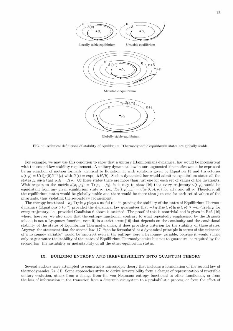
In order to implement Condition 5 above, we need to establish the relation between the notion of stability impliedby the second law of Thermodynamics [5, 11] (and reviewed in Section 2) and the mathematical concept of stability.An equilibrium state is stable, in the sense required by the second law, if it can be altered to a different state only byinteractions that leave net effects in the state of the enviromment. We call this notion of stability global stability. Thenotion of stability according to Lyapunov is called local stability. In this Section we review the technical definitions.

We denote the trajectories generated by the dynamical law on our state domain by u(t, ρ), i.e., u(t, ρ) denotes thestate at time t along the trajectory that at time t = 0 passes through state ρ. A state ρe is an equilibrium state ifand only if u(t, ρe) = ρe for all times t. As sketched in Figure 2, an equilibrium state ρe is locally stable (according toLyapunov) if and only if for every ε > 0 there is a δ(ε) > 0 such that d(ρ, ρe) < δ(ε) implies d(u(t, ρ), ρe) < ε for allt > 0 and every ρ, i.e., such that every trajectory that passes within the distance δ(ε) from state ρe proceeds in timewithout ever exceeding the distance ε from ρe. Conversely, an equilibrium state ρe is unstable if and only if it is notlocally stable, i.e., there is an ε > 0 such that for every δ > 0 there is a trajectory passing within distance δ from ρeand reaching at some later time farther than the distance ε from ρe.

The Lyapunov concept of instability of equilibrium is clearly equivalent to that of instability stated in Thermody-namics according to which an equilibrium state is unstable if, upon experiencing a minute and short lived influenceby some system in the environment (i.e., just enough to take it from state ρe to a neighboring state at infinitesimaldistance δ), proceeds from then on spontaneously to a sequence of entirely different states (i.e., farther than somefinite distance ε).

It follows that the concept of stability in Thermodynamics implies that of Lyapunov local stability. However, it isstronger because it also excludes the concept of metastability. Namely, the states of Equilibrium Thermodynamicsare global stable equilibrium states in the sense that not only they are locally stable but they cannot be altered toentirely different states even by means of interactions which leave temporary but finite effects in the environment.Mathematically, the concept of metastability can be defined as follows. An equilibrium state ρe is metastable if andonly if it is locally stable but there is an η > 0 and an ε > 0 such that for every δ > 0 there is a trajectory u(t, ρ)passing at t = 0 between distance η and η + δ from ρe, η < d(u(0, ρ), ρe) < η + δ, and reaching at some later timet > 0 a distance farther than η + ε, d(u(t, ρ), ρe) ≥ η + ε. Thus, the concept of global stability implied by the secondlaw is as follows. An equilibrium state ρe is globally stable if for every η > 0 and every ε > 0 there is a δ(ε, η) > 0such that every trajectory u(t, ρ) with η < d(u(0, ρ), ρe) < η + δ(ε, η), i.e., passing at time t = 0 between distance ηand η + δ from ρe, remains with d(u(t, ρ), ρe) > η + ε for every t > 0, i.e., proceeds in time without ever exceedingthe distance η + ε.

The second law requires that for each set of values of the invariants TrHρ and TrNiρ (as many as required by thestructure of the system), and of the parameters describing the external forces (such as the size of a container), thereis one and only one globally stable equilibrium state. Thus, the dynamical law may admit many equilibrium statesthat all share the same values of the invariants and the parameters, but among all these only one is globally stable,i.e., all the other equilibrium states are either unstable or metastable.

12

�e

�����

Locally stable equilibrium

�e

��

Unstable equilibrium

�e

�’��’�

Metastable equilibrium

������

�e

Globally stable equilibrium

�

�’ �

�����������

FIG. 2: Technical definitions of stability of equilibrium. Thermodynamic equilibrium states are globally stable.

For example, we may use this condition to show that a unitary (Hamiltonian) dynamical law would be inconsistentwith the second-law stability requirement. A unitary dynamical law in our augmented kinematics would be expressedby an equation of motion formally identical to Equation 11 with solutions given by Equation 13 and trajectoriesu(t, ρ) = U(t)ρ(0)U−1(t) with U(t) = exp(−itH/�). Such a dynamical law would admit as equilibrium states all thestates ρe such that ρeH = Hρe. Of these states there are more than just one for each set of values of the invariants.With respect to the metric d(ρ1, ρ2) = Tr|ρ1 − ρ2|, it is easy to show [16] that every trajectory u(t, ρ) would beequidistant from any given equilibrium state ρe, i.e., d(u(t, ρ), ρe) = d(u(0, ρ), ρe) for all t and all ρ. Therefore, allthe equilibrium states would be globally stable and there would be more than just one for each set of values of theinvariants, thus violating the second-law requirement.

The entropy functional −kB Trρ ln ρ plays a useful role in proving the stability of the states of Equilibrium Thermo-dynamics (Equations 5 to 7) provided the dynamical law guarantees that −kB Tru(t, ρ) lnu(t, ρ) ≥ −kB Trρ ln ρ forevery trajectory, i.e., provided Condition 6 above is satisfied. The proof of this is nontrivial and is given in Ref. [16]where, however, we also show that the entropy functional, contrary to what repeatedly emphasized by the Brusselsschool, is not a Lyapunov function, even if, in a strict sense [16] that depends on the continuity and the conditionalstability of the states of Equilibrium Thermodynamics, it does provide a criterion for the stability of these states.Anyway, the statement that the second law [17] “can be formulated as a dynamical principle in terms of the existenceof a Lyapunov variable” would be incorrect even if the entropy were a Lyapunov variable, because it would sufficeonly to guarantee the stability of the states of Equilibrium Thermodynamics but not to guarantee, as required by thesecond law, the instability or metastability of all the other equilibrium states.

IX. BUILDING ENTROPY AND IRREVERSIBILITY INTO QUANTUM THEORY

Several authors have attempted to construct a microscopic theory that includes a formulation of the second law ofthermodynamics [24–31]. Some approaches strive to derive irreversibility from a change of representation of reversibleunitary evolution, others from a change from the von Neumann entropy functional to other functionals, or fromthe loss of information in the transition from a deterministic system to a probabilistic process, or from the effect of

13

coupling with one or more heat baths.We discuss the key elements and features of a different non-standard theory which introduces de facto an ansatz of

“intrinsic entropy and instrinsic irreversibility” at the fundamental level [2, 32], and an additional ansatz of “steepestentropy ascent” which entails an explicit well-behaved dynamical principle and the second law of thermodynamics.To present it, we first discuss an essential fundamental concept.

X. STATES OF A STRICTLY ISOLATED INDIVIDUAL SYSTEM

Let us consider a system A and denote by R the rest of the universe, so that the Hilbert space of the universe isHAR = HA⊗HR. We restrict our attention to a “strictly isolated” system A, by which we mean that at all times,−∞ < t < ∞, A is uncorrelated (and hence disentangled) from R, i.e., ρAR = ρA⊗ρR, and non-interacting, i.e.,HAR = HA⊗IR + IA⊗HR.

Many would object at this point that with this premise the following discussion should be dismissed as uselessand unnecessary, because no “real” system is ever strictly isolated. We reject this argument as counterproductive,misleading and irrelevant, for we recall that Physics is a conceptual edifice by which we attempt to model and unifyour perceptions of the empirical world (physical reality [33]). Abstract concepts such as that of a strictly isolatedsystem and that of a state of an individual system not only are well-defined and conceivable, but have been keystonesof scientific thinking, indispensable for example to structure the principle of causality. In what other framework couldwe introduce, say, the time-dependent Schrodinger equation?

Because the dominant theme of quantum theory is the necessity to accept that the notion of state involves prob-abilistic concepts in an essential way [34], established practices of experimental science impose that the construct“probability” be linked to the relative frequency in an “ensemble”. Thus, the purpose of a quantum theory is to reg-ularize purely probabilistic information about the measurement results from a “real ensemble” of identically preparedidentical systems. An important scheme for the classification of ensembles, especially emphasized by von Neumann[35], hinges upon the concept of ensemble “homogeneity”. Given an ensemble it is always possible to conceive of itas subdivided into many sub-ensembles. An ensemble is homogeneous iff every conceivable subdivision results intosub-ensembles all identical to the original (two sub-ensembles are identical iff upon measurement on both of the samephysical observable at the same time instant, the outcomes yield the same arithmetic mean, and this holds for allconceivable physical observables). It follows that each individual member system of a homogeneous ensemble hasexactly the same intrinsic characteristics as any other member, which therefore define the “state” of the individualsystem. In other words, the empirical correspondent of the abstract concept of “state of an individual system” is thehomogeneous ensemble (sometimes also called “pure” [36–38] or “proper” [39, 40]).

We restrict our attention to the states of a strictly isolated individual system. By this we rule out from ourpresent discussion all heterogeneous preparations, such as those considered in QSM and QIT, which are obtained bystatistical composition of different homogeneous component preparations. Therefore, we concentrate on the intrinsiccharacteristics of each individual system and their irreducible, non-statistical probabilistic nature.

XI. BROADER QUANTUM KINEMATICS ANSATZ

According to standard QM the states of a strictly isolated individual system are in one-to-one correspondence withthe one-dimensional orthogonal projection operators on the Hilbert space of the system. We denote such projectorsby the symbol P . If |ψ〉 is an eigenvector of P such that P |ψ〉 = |ψ〉 and 〈ψ|ψ〉 = 1 then P = |ψ〉〈ψ|. It is well knownthat differently from classical states, quantum states are characterized by irreducible intrinsic probabilities. We neednot elaborate further on this point. We only recall that −TrP lnP = 0.

Instead, we adhere to the ansatz [11] that the set of states in which a strictly isolated individual system may befound is broader than conceived in QM, specifically that it is in one-to-one correspondence with the set of linearoperators ρ on H, with ρ† = ρ, ρ > 0, Trρ = 1, without the restriction ρ2 = ρ. We call these the “state operators”to emphasize that they play the same role that in QM is played by the projectors P , and that they are associatedwith the homogeneous preparation schemes. This fundamental ansatz has been first proposed by Hatsopoulos andGyftopoulos [11]. It allows an implementation of the second law of thermodynamics at the fundamental level in whichthe physical entropy, given by s(ρ) = −kBTrρ lnρ, emerges as an intrinsic microscopic and non-statistical property ofmatter, in the same sense as the (mean) energy e(ρ) = TrρH is an intrinsic property.

We first assume that our isolated system is an indivisible constituent of matter, i.e., one of the following:

• A single strictly isolated d-level particle, in which case H = Hd = ⊕dk=0Hekwhere ek is the k-th eigenvalue of

the (one-particle) Hamiltonian H1 and Hekthe corresponding eigenspace). Even if the system is isolated, we

14

do not rule out fluctuations in energy measurement results and hence we do not assume a “microcanonical”Hamiltonian (i.e., H = ekPHe

kfor some k) but we assume a full “canonical” HamiltonianH = H1 =

∑k ekPHek

.

• A strictly isolated ideal Boltzmann gas of non-interacting identical indistinguishable d-level particles, in whichcase H is a Fock space, H = Fd = ⊕∞

n=0H⊗nd . Again, we do not rule out fluctuations in energy nor in the number

of particles, and hence we do not assume a canonical number operator (i.e., N = zPH⊗zd

for some z) but weassume a full grand canonical number operator N =

∑∞n=0 nPH⊗n

dand a full Hamiltonian H =

∑∞n=0HnPH⊗n

d

where Hn =∑nJ=1(H1)J⊗IJ is the n-particle Hamiltonian on H⊗n

d , (H1)J denotes the one-particle Hamiltonianon the J-th particle space (Hd)J and IJ the identity operator on the direct product space ⊗nK=1,K �=J(Hd)K ofall other particles. Note that [H,N ] = 0.

• A strictly isolated ideal Fermi-Dirac or Bose-Einstein gas of non-interacting identical indistinguishable d-levelparticles, in which case H is the antisymmetric or symmetric subspace, respectively, of the Boltzmann Fockspace just defined.

We further fix ideas by considering the simplest quantum system, a 2-level particle, a qubit. It is well known [21]that using the 3-vector σ = (σ1, σ2, σ3) of Pauli spin operators, [σj , σk] = εjk�σ�, we can represent the Hamiltonianoperator as H = �ω( 1

2I + h ·σ) where h is a unit-norm 3-vector of real scalars (h1, h2, h3), and the density operatorsas ρ = 1

2I + r · σ where r is a 3-vector of real scalars (r1, r2, r3) with norm r = |r| ≤ 1, and r = 1 iff ρ is idempotent,ρ2 = ρ.

If the 2-level particle is strictly isolated, its states in standard QM are one-to-one with the unit-norm vectorsψ in H or, equivalently, the unit-trace one-dimensional projection operators on H, Pψ = |ψ〉〈ψ|ψ〉−1〈ψ|, i.e., theidempotent density operators ρ2 = ρ. Hence, in the 3-dimensional euclidean space (r1, r2, r3), states map one-to-onewith points on the unit radius 2-dimensional spherical surface, r = 1, the “Bloch sphere”. The mean value of theenergy is e(ρ) = TrρH = 1

2 (1 + h · r) and is clearly bounded by 0 ≤ e(ρ) ≤ �ω. The set of states that share a givenmean value of the energy are represented by the 1-dimensional circular intersection between the Bloch sphere and theconstant mean energy plane orthogonal to h defined by the h · r = const condition. The time evolution accordingto the Schrodinger equation ψ = −iHψ/� or, equivalently, Pψ = −i[H,Pψ]/� or [21] r = ωh × r yields a periodicprecession of r around h along such 1-dimensional circular path on the surface of the Bloch sphere. At the end ofevery (Poincar) cycle the strictly isolated system passes again through its initial state: a clear pictorial manifestationof the reversibility of Hamiltonian dynamics.

At the level of a strictly isolated qubit, the Hatsopoulos-Gyftopoulos ansatz amounts to accepting that the two-levelsystem admits also states that must be described by points inside the Bloch sphere, not just on its surface, even ifthe qubit is noninteracting and uncorrelated. The eigenvalues of ρ are (1± r)/2, therefore the isoentropic surfaces areconcentric spheres,

s(ρ) = s(r) = −kB

(1 + r

2ln

1 + r

2+

1 − r

2ln

1 − r

2

). (1)

The highest entropy state with given mean energy is at the center of the disk obtained by intersecting the Blochsphere with the corresponding constant energy plane. Such states all lie on the diameter along the direction of theHamiltonian vector h and are thermodynamic equilibrium (maximum entropy principle [7]).

Next, we construct our extension of the Schrodinger equation of motion valid inside the Bloch sphere. By assumingsuch law of causal evolution, the second law will emerge as a theorem of the dynamics.

XII. STEEPEST-ENTROPY-ASCENT ANSATZ

Let us return to the general formalism for a strictly isolated system. We go back to the qubit example at the endof the section.

As a first step to force positivity and hermiticity of the state operator ρ we assume an equation of motion of theform

dρdt

= ρE(ρ) + E†(ρ) ρ =√ρ

(√ρE(ρ)

)+

(√ρE(ρ)

)†√ρ , (2)

where E(ρ) is a (non-hermitian) operator-valued (nonlinear) function of ρ that we call the “evolution” operator.Without loss of generality, we write E = E+ + iE− where E+ = (E + E†)/2 and E− = (E − E†)/2i are hermitianoperators, so that Eq. (2) takes the form

dρdt

= −i[E−(ρ), ρ] + {E+(ρ), ρ} , (3)

15

with [ · , · ] and { · , · } the usual commutator and anti-commutator, respectively.We consider the real space of linear (not necessarily hermitian) operators on H equipped with the real scalar product

(F |G) = Tr(F †G+G†F )/2 , (4)

so that for any time-independent hermitian observable X on H, the rate of change of the mean value x(ρ) = Tr(ρX) =(√ρ|√ρX) can be written as

dr(ρ)dt

= Tr(dρdtX) = 2 (

√ρE| √ρX) , (5)

from which it follows that a set of xi(ρ)’s is time invariant iff√ρE is orthogonal to the (real) linear span of the set

of operators√ρXi, that we denote by L{√ρXi}.

For an isolated system, we therefore require that, for every ρ, operator√ρE be orthogonal [in the sense of scalar

product (4)] to the linear manifold L(√ρI, {√ρRi}) where the set

√ρI, {√ρRi} always includes

√ρI, to preserve

Trρ = 1, and√ρH , to conserve the mean energy e(ρ) = TrρH . For a field of indistinguishable particles we also

include√ρN to conserve the mean number of particles n(ρ) = TrρN . For a free particle we would include

√ρPx,√

ρPy,√ρPz to conserve the mean momentum vector p(ρ) = TrρP, but here we omit this case for simplicity [47].

Similarly, the rate of change of the entropy functional can be written as

ds(ρ)dt

= (√ρE |−2kB [

√ρ+

√ρ ln ρ] ) , (6)

where the operator −2kB

[√ρ+

√ρ ln ρ

]may be interpreted as the gradient (in the sense of the functional derivative)

of the entropy functional s(ρ) = −kBTrρ ln ρ with respect to operator√ρ (for the reasons why in our theory the

physical entropy is represented by the von Neumann functional, see Refs. [11, 41]).It is noteworthy that the Hamiltonian evolution operator

EH = iH/� , (7)

is such that√ρEH is orthogonal to L(

√ρI,

√ρH(,

√ρN)) as well as to the entropy gradient operator

−2kB

[√ρ+

√ρ ln ρ

]. It yields a Schrodinger-Liouville-von Neumann unitary dynamics

dρdt

= ρEH + E†Hρ = − i

�[H, ρ] , (8)

which maintains time-invariant all the eigenvalues of ρ. Because of this feature, all time-invariant (equilibrium) densityoperators according to Eq. (8) (those that commute with H) are globally stable [16] with respect to perturbationsthat do not alter the mean energy (and the mean number of particles). As a result, for given values of the meanenergy e(ρ) and the mean number of particles n(ρ) such a dynamics would in general imply many stable equilibriumstates, contrary to the second law requirement that there must be only one (this is the well-known Hatsopoulos-Keenan statement of the second law [42], which entails [7] the other well-known statements by Clausius, Kelvin, andCaratheodory).

Therefore, we assume that in addition to the Hamiltonian term EH , the evolution operator E has an additionalcomponent ED,

E = EH + ED , (9)

that we will take so that√ρED is at any ρ orthogonal both to

√ρEH and to the intersection of the linear manifold

L(√ρI, {√ρRi}) with the isoentropic hypersurface to which ρ belongs (for a two level system, such intersection is a

one-dimensional planar circle inside the Bloch sphere). In other words, we assume that√ρED is proportional to the

component of the entropy gradient operator −2kB

[√ρ+

√ρ ln ρ

]orthogonal to L(

√ρI, {√ρRi}),

√ρED = − 1

2τ(ρ)[√ρ ln ρ]⊥L(

√ρI,

√ρH(,

√ρN)) , (10)

where we denote the “constant” of proportionality by 1/2τ(ρ) and use the fact that√ρ has no component orthogonal

to L(√ρI,

√ρH(,

√ρN)).

It is important to note that the “intrinsic dissipation” or “intrinsic relaxation” characteristic time τ(ρ) is leftunspecified in our construction and need not be a constant. All our results hold as well if τ(ρ) is some reasonably wellbehaved positive definite functional of ρ. The empirical and/or theoretical determination of τ(ρ) is a most challenging

16

open problem in our research program. For example, it has been suggested [43] that the experiments by Franzen[44] (intended to evaluate the spin relaxation time constant of vapor under vanishing pressure conditions) and byKukolich [45] (intended to provide a laboratory validation of the time-dependent Schrodinger equation) both suggestsome evidence of an intrinsic relaxation time.

Using standard geometrical notions, we can show [2, 19, 32, 46] that given any set of linearly independent operators√ρI, {√ρRi} spanning L(

√ρI,

√ρH(,

√ρN)) the dissipative evolution operator takes the explicit expression

√ρED =

12kBτ(ρ)

√ρ∆M(ρ) (11)

where M(ρ) is a “Massieu-function” operator defined by the following ratio of determinants

M(ρ) =

∣∣∣∣∣∣∣∣∣∣∣∣∣∣∣

S I · · · Ri · · ·

(√ρS|√ρI) (

√ρI|√ρI) · · · (

√ρRi|√ρI) · · ·

......

. . ....

. . .(√ρS|√ρRi) (

√ρI|√ρRi) · · · (

√ρRi|√ρRi) · · ·

......

. . ....

. . .

∣∣∣∣∣∣∣∣∣∣∣∣∣∣∣Γ(

√ρI, {√ρRi}) , (12)

in which we use the following notation (F , G hermitian)

S = −kBPRan ρ ln ρ , (13)∆F = F − Tr(ρF )I , (14)

〈∆F∆G〉 = (√ρ∆F |√ρ∆G) =

12Tr(ρ{∆F,∆G}) , (15)

Γ(√ρI, {√ρRi}) = Γ({√ρ∆Ri}) = det[〈∆Ri∆Rj〉] , (16)

where Γ({√ρXi}) denotes the Gram determinant det[(√ρXi|√ρXj)].

The Massieu-function operator defined by Eq. (12) generalizes to any non-equilibrium state the well-known equi-librium Massieu characteristic function s(ρTE) − β e(ρTE) [+βµn(ρTE)].

As a result, our full equation of motion

dρdt

= − i

�[H, ρ] +

12kBτ(ρ)

{∆M(ρ), ρ} (17)

takes the form

dρdt

= − i

�[H, ρ] +

12kBτ(ρ)

∣∣∣∣∣∣∣∣∣∣∣∣∣∣∣

{∆S, ρ} {∆R1, ρ} · · · {∆Ri, ρ} · · ·

〈∆S∆R1〉 〈∆R1∆R1〉 · · · 〈∆Ri∆R1〉 · · ·...

.... . .

.... . .

〈∆S∆Ri〉 〈∆R1∆Ri〉 · · · 〈∆Ri∆Ri〉 · · ·...

.... . .

.... . .

∣∣∣∣∣∣∣∣∣∣∣∣∣∣∣det[〈∆Ri∆Rj〉] . (18)

Equations (28) and (29) below show the explicit forms when the set {√ρRi} is empty or contains only operator√ρH ,

respectively.Gheorghiu-Svirschevski [47] re-derived our nonlinear equation of motion from a variational principle that in our

notation may be cast as follows [19],

max√ρED

ds(ρ)dt

subject todri(ρ)

dt= 0 and (

√ρED|

√ρED) = c2(ρ) , (19)

where r0(ρ) = Trρ, r1(ρ) = TrHρ [, r2(ρ) = TrNρ], and c2(ρ) is some positive functional. The last constraint meansthat we are not really searching for “maximal entropy production” but only for the direction of steepest entropy ascent,

17

leaving unspecified the rate at which such direction “attracts” the state of the system. The necessary condition interms of Lagrange multipliers is

∂

∂√ρED

dsdt

−∑i

λi∂

∂√ρED

dridt

− λ0∂

∂√ρED

(√ρED|

√ρED) = 0 , (20)

and, using Eqs. (5) and (6) becomes

−2kB(√ρ+

√ρ ln ρ) − 2

∑λi√ρRi − 2λ0

√ρED = 0 , (21)

which inserted in the constraints and solved for the multipliers yields Eq. (11).The resulting rate of entropy change (entropy generation by irreversibility, for the system is isolated) is given by

the equivalent expressions

ds(ρ)dt

= −kB

dTrρ ln ρdt

= 4kBτ(ρ) (√ρED |√ρED ) (22)

=kB

τ(ρ)Γ(

√ρ ln ρ,

√ρI, {√ρRi})

Γ(√ρI, {√ρRi}) (23)

=1

kBτ(ρ)Γ(

√ρS,

√ρI, {√ρRi})

Γ(√ρI, {√ρRi}) ≥ 0 . (24)

Because a Gram determinant Γ(√ρX1, . . . ,

√ρXN ) = det[〈∆Xi∆Xj〉] is either strictly positive or zero iff operators

{√ρXi} are linearly dependent, the rate of entropy generation is either a positive semi-definite nonlinear functionalof ρ, or it is zero iff operators

√ρS,

√ρI,

√ρH(,

√ρN) are linearly dependent, i.e., iff the state operator is of the form

ρ =B exp[−βH (+νN)]B

Tr(B exp[−βH (+νN)]), (25)

for some “binary” projection operator B (B2 = B, eigenvalues either 0 or 1) and some real scalar(s) β (and ν). Non-dissipative states are therefore all and only the density operators that have the nonzero eigenvalues “canonically” (or“grand canonically”) distributed. For them,

√ρED = 0 and our equation of motion (17) reduces to the Schrodinger–

von Neumann form i�ρ = [H, ρ]. Such states are either equilibrium states, if [B,H ] = 0, or belong to a limit cycleand undergo a unitary hamiltonian dynamics, if [B,H ] �= 0, in which case

ρ(t) = B(t) exp[−βH (+νN)]B(t)/Tr[B(t) exp[−βH (+νN)]] , (26)B(t) = U(t)B(0)U−1(t) , U(t) = exp(−itH/�) . (27)

For TrB = 1 the states (25) reduce to the (zero entropy) states of standard QM, and obey the standard unitarydynamics generated by the usual time-dependent Schrodinger equation. For B = I we have the maximal-entropy(thermodynamic-equilibrium) states, which turn out to be the only globally stable equilibrium states of our dynamics,so that the Hatsopoulos-Keenan statement of the second law emerges as an exact and general dynamical theorem.

Indeed, in the framework of our extended theory, all equilibrium states and limit cycles that have at least one nulleigenvalue of ρ are unstable. This is because any neighboring state operator with one of the null eigenvalues perturbed(i.e., slightly “populated”) to a small value ε (while some other eigenvalues are slightly changed so as to ensure thatthe perturbation preserves the mean energy and the mean number of constituents), would eventually proceed “faraway” towards a new partially-maximal-entropy state or limit cycle with a canonical distribution which fully involvesalso the newly “populated” eigenvalue while the other null eigenvalues remain zero.

It is clear that the canonical (grand-canonical) density operators ρTE = exp[−βH (+νN)]/Tr(exp[−βH (+νN)])are the only stable equilibrium states, i.e., the TE states of the strictly isolated system. They are mathematicallyidentical to the density operators which also in QSM and QIT are associated with TE, on the basis of their maximizingthe von Neumann indicator of statistical uncertainty −Trρ ln ρ subject to given values of TrHρ (and TrNρ). Becausemaximal entropy mathematics in QSM and QIT successfully represents TE physical reality, our theory, by entailing thesame mathematics for the stable equilibrium states, preserves all the successful results of equilibrium QSM and QIT.However, within QT such mathematics takes up an entirely different physical meaning. Indeed, each density operatorhere does not represent statistics of measurement results from a “heterogeneous” ensemble, as in QSM and QIT where,according to von Neumann’s recipe [35, 48], the “intrinsic” uncertainties (irreducibly introduced by standard QM) aremixed with the “extrinsic” uncertainties (related to the heterogeneity of its preparation, i.e., to not knowing the exactstate of each individual system in the ensemble). In QT, instead, each density operator, including the maximal-entropy

18

stable TE ones, represents “intrinsic” uncertainties only, because it is associated with a homogeneous preparation and,therefore, it represents the state of each and every individual system of the homogeneous ensemble.

We noted elsewhere [49] that the fact that our nonlinear equation of motion preserves the null eigenvalues of ρ, i.e.,conserves the cardinality dim Ker(ρ) of the set of zero eigenvalues, is an important physical feature consistent withrecent experimental tests (see the discussion of this point in Ref. [47] and references therein) that rule out, for pure(zero entropy) states, deviations from linear and unitary dynamics and confirm that initially unoccupied eigenstatescannot spontaneously become occupied. This fact, however, adds nontrivial experimental and conceptual difficultiesto the problem of designing fundamental tests capable, for example, of ascertaining whether decoherence originatesfrom uncontrolled interactions with the environment due to the practical impossibility of obtaining strict isolation, orelse it is a more fundamental intrinsic feature of microscopic dynamics requiring an extension of QM like the one wepropose.

For a confined, strictly isolated d-level system, our equation of motion for non-zero entropy states (ρ2 �= ρ) takesthe following forms [21, 50]. If the Hamiltonian is fully degenerate [H = eI, e(ρ) = e for every ρ],

dρdt

= − i

�[H, ρ] − 1

τ(ρ lnρ− ρTrρ ln ρ) , (28)

while if the Hamiltonian is nondegenerate,

dρdt

= − i

�[H, ρ] − 1

τ

∣∣∣∣∣∣∣∣∣∣

ρ lnρ ρ 12{H, ρ}

Trρ ln ρ 1 TrρH

TrρH ln ρ TrρH TrρH2

∣∣∣∣∣∣∣∣∣∣TrρH2 − (TrρH)2

.

In particular, for a non-degenerate two-level system, it may be expressed in terms of the Bloch sphere representation(for 0 < r < 1) as [21]

r = ωh× r − 1τ

(1 − r2

2rln

1 − r

1 + r

)h × r × h1 − (h · r)2 (29)

from which it is clear that the dissipative term lies in the constant mean energy plane and is directed towards theaxis of the Bloch sphere identified by the Hamiltonian vector h. The nonlinearity of the equation does not allow ageneral explicit solution, but on the central constant-energy plane, i.e., for initial states with r · h = 0, the equationimplies [21]

ddt

ln1 − r

1 + r= −1

τln

1 − r

1 + r(30)

which, if τ is constant, has the solution

r(t) = tanh[− exp

(− t

τ

)ln

1 − r(0)1 + r(0)

]. (31)

This, superposed with the precession around the hamiltonian vector, results in a spiraling approach to the maximalentropy state (with entropy kB ln 2). Notice, that the spiraling trajectory is well-defined and within the Bloch spherefor all times −∞ < t < +∞, and if we follow it backwards in time it approaches as t → −∞ the limit cycle whichrepresents the standard QM (zero entropy) states evolving according to the Schrodinger equation.

This example shows quite explicitly a general feature of our nonlinear equation of motion which follows from theexistence and uniqueness of its solutions for any initial density operator both in forward and backward time. Thisfeature is a consequence of two facts: (1) that zero eigenvalues of ρ remain zero and therefore no eigenvalue cancross zero and become negative, and (2) that Trρ is preserved and therefore if initially one it remains one. Thus, theeigenvalues of ρ remain positive and less than unity. On the conceptual side, it is also clear that our theory implementsa strong causality principle by which all future as well as all past states are fully determined by the present stateof the isolated system, and yet the dynamics is physically (thermodynamically) irreversible. Said differently, if weformally represent the general solution of the Cauchy problem by ρ(t) = Λtρ(0) the nonlinear map Λt is a group, i.e.,Λt+u = ΛtΛu for all t and u, positive and negative. The map is therefore “invertible”, in the sense that Λ−t = Λ−1

t ,where the inverse map is defined by ρ(0) = Λ−1

t ρ(t).

19

It is a nontrivial observation that the non-invertibility of the dynamical map is not at all necessary to represent aphysically irreversible dynamics. Yet, innumerable attempts to build irreversible theories start from the assertion thatin order to represent thermodynamic irreversibility the dynamical map should be non-invertible. The arrow of timein our view is not to be sought for in the impossibility to retrace past history, but in the spontaneous tendency of anyphysical system to internally redistribute its energy (and, depending on the system, its other conserved propertiessuch number of particles, momentum, angular momentum) along the path of steepest entropy ascent.

XIII. ONSAGER RECIPROCITY

The intrinsically irreversible dynamics entailed by the dissipative (non-hamiltonian) part of our nonlinear equationof motion also entails an Onsager reciprocity theorem. To see this, we first note that any density operator ρ can bewritten as [20]

ρ =B exp(−∑

j fjXj)BTrB exp(−∑

j fjXj), (32)

where the possibly time-dependent Boolean B is such that B = PRanρ (= I − PKerρ) and the time-independentoperators Xj together with the identity I form a set such that their restrictions to H′ = BH, {I ′, X ′

j} span the realspace of hermitian operators on H′ = BH. Hence,

√ρ ln ρ = −f0√ρ−

∑j fj

√ρXj , (33)

xj(ρ) = Tr(ρXj) , (34)s(ρ) = kBf0 + kB

∑j fj xj(ρ) , (35)

where kBfj =∂s(ρ)∂xj(ρ)

∣∣∣∣xi�=j(ρ)

(36)

may be interpreted as a “generalized affinity” or force. Defining

Dxi(ρ)Dt

= 2(ED|√ρXi) . (37)

as “the dissipative rate of change” of the mean value xj(ρ), we find

Dxi(ρ)Dt

=∑j

fj Lij(ρ) , (38)

where the coefficients Lij(ρ) (nonlinear in ρ) may be interpreted as “generalized conductivities” and are given explicitly(no matter how far ρ is from TE) by

Lij(ρ) =1

τ(ρ)([√ρXi]⊥L(

√ρI,{√ρRi})

∣∣ [√ρXj ]⊥L(

√ρI,{√ρRi})

)(39)

=1

τ(ρ)

∣∣∣∣∣∣∣∣∣∣∣∣∣∣∣

〈∆Xi∆Xj〉 〈∆R1∆Xj〉 · · · 〈∆Rk∆Xj〉 · · ·

〈∆Xi∆R1〉 〈∆R1∆R1〉 · · · 〈∆Rk∆R1〉 · · ·...

.... . .

.... . .

〈∆Xi∆Rk〉 〈∆R1∆Rk〉 · · · 〈∆Rk∆Rk〉 · · ·...

.... . .

.... . .

∣∣∣∣∣∣∣∣∣∣∣∣∣∣∣det[〈∆Rk∆R�〉] = Lji(ρ) , (40)

and therefore form a symmetric, non-negative definite Gram matrix [Lij(ρ)], which is strictly positive iff all operators[√ρXi]⊥L(

√ρI,{√ρRi}) are linearly independent.

The rate of entropy generation may be rewritten as a quadratic form of the generalized affinities,

ds(ρ)dt

= kB

∑i

∑j

fifjLij(ρ) . (41)

20

If all operators [√ρXi]⊥L(

√ρI,{√ρRi}) are linearly independent, det[Lij(ρ)] �= 0 and Eq. (38) may be solved to yield

fj =∑i

L−1ij (ρ)

Dxi(ρ)Dt

, (42)

and the rate of entropy generation can be written also as a quadratic form of the dissipative rates

ds(ρ)dt

= kB

∑i

∑j

L−1ij (ρ)

Dxi(ρ)Dt

Dxj(ρ)Dt

. (43)

XIV. COMPOSITE SYSTEMS AND REDUCED DYNAMICS

The composition of the system is embedded in the structure of the Hilbert space as a direct product of the subspacesassociated with the individual elementary constituent subsystems, as well as in the form of the Hamiltonian operator.In this section, we consider a system composed of distinguishable and indivisible elementary constituent subsystems.For example:

• A strictly isolated composite of r distinguishable d-level particles, in which case H = ⊗rJ=1HdJ and H =∑rJ=1(H1)J ⊗ IJ + V where V is some interaction operator over H.

• A strictly isolated ideal mixture of r types of Boltzmann, Fermi-Dirac or Bose-Einstein gases of non-interactingidentical indistinguishable dJ -level particles, J = 1, . . . , r, in which case H is a composite of Fock spacesH = ⊗rJ=1FdJ = ⊕∞

n1=0 · · ·⊕∞nr=0H⊗n1

d1⊗· · ·⊗H⊗nr

drwhere the factor Fock spaces belonging to Fermi-Dirac (Bose-

Einstein) components are restricted to their antisymmetric (symmetric) subspaces. Again, we assume full grand-canonical number operators NJ =

∑∞nJ=0 nJPH⊗nJ

dJ

and Hamiltonian H =∑r

J=1 IJ ⊗ ∑∞nJ=0HnJPH⊗nJ

dJ

+ V .

For compactness of notation we denote the subsystem Hilbert spaces as

H = H1⊗H2⊗ · · ·⊗Hr = HJ⊗HJ , (44)

where J denotes all subsystems except the J-th one. The overall system is strictly isolated in the sense alreadydefined, and the Hamiltonian operator

H =r∑

J=1

HJ⊗IJ + V , (45)

where HJ is the Hamiltonian on HJ associated with the J-th subsystem when isolated and V (on H) the interactionHamiltonian among the r subsystems.

The subdivision into elementary constituents, considered as indivisible, and reflected by the structure of the Hilbertspace H as a direct product of subspaces, is particularly important because it defines the level of description of thesystem and specifies its elementary structure. The system’s internal structure we just defined determines the form ofthe nonlinear dynamical law proposed by this author [18, 19, 46] to implement the steepest entropy ascent ansatz ina way compatible with the obvious self-consistency “separability” and “locality” requirements [49]. It is importantto note that, because our dynamical principle is nonlinear in the density operator, we cannot expect the form of theequation of motion to be independent of the system’s internal structure.

The equation of motion that we “designed” in [18, 46] so as to guarantee all the necessary features (that we list inRef. [49]), is

dρdt

= − i

�[H, ρ] +

r∑J=1

12kBτJ(ρ)

{(∆MJ(ρ))J , ρJ}⊗ρJ , (46)

where we use the notation [see Ref. [19] for interpretation of (S)J and (H)J ]

√ρJ (MJ(ρ))J =

[√ρJ (S)J

]⊥L(

√ρJ IJ ,

√ρJ (HJ )J (,

√ρJ (NkJ)J ))

, (47)

(FJ |GJ)J = TrJ(F †JGJ +G†

JFJ )/2 , (48)

(RiJ )J = TrJ [(IJ⊗ρJ)RiJ ] , (49)

(S)J = TrJ [(IJ⊗ρJ)S] , (50)

21

and the “internal redistribution characteristic times” τJ(ρ)’s are some positive constants or positive functionals of theoverall system’s density operator ρ.

All the results found for the single constituent extend in a natural way to the composite system. For example, therate of entropy change becomes

ds(ρ)dt

=r∑

J=1

1kBτJ (ρ)

Γ(√ρJ(S)J ,√ρJIJ , {√ρJ(RiJ )J})Γ(√ρJIJ , {

√ρJ(RiJ )J}) . (51)

The dynamics reduces to the Schrodinger-von Neumann unitary Hamiltonian dynamics when, for each J , there aremultipliers λiJ such that

√ρJ(S)J =

√ρJ

∑i

λiJ (RiJ )J . (52)

The equivalent variational formulation is

max{√ρJEDJ}

ds(ρ)dt

subject todri(ρ)

dt= 0 and (

√ρJEDJ |

√ρJEDJ )J = c2

J(ρ) , (53)

where r0(ρ) = Trρ, r1(ρ) = TrHρ [, r2(ρ) = TrNρ], and c2J(ρ) are some positive functionals of ρ. The last constraints,

one for each subsystem, mean that each subsystem contributes to the overall evolution (for the dissipative non-hamiltonian part) by pointing towards its “local perception” of the direction of steepest (overall) entropy ascent, eachwith an unspecified intensity (which depends on the values of the functionals cJ (ρ), that are inversely related to theinternal redistribution characteristic times τJ(ρ)).

If two subsystems A and B are non-interacting but in correlated states, the reduced state operators obey theequations

dρAdt

= − i

�[HA, ρA] +

1kB

r∑J=1J∈A

12τJ(ρ)

{(∆MJ(ρ))J , ρJ}⊗(ρA)J , (54)

dρBdt

= − i

�[HB, ρB] +

1kB

r∑J=1J∈B

12τJ (ρ)

{(∆MJ(ρ))J , ρJ}⊗(ρB)J , (55)

where (ρA)J = TrJ (ρA), (ρB)J = TrJ (ρB), and operators (∆MJ (ρ))J result independent of HB for every J ∈ Aand independent of HA for every J ∈ B. Therefore, all functionals of ρA (local observables) remain unaffected bywhatever change in B, i.e., locality problems are excluded.

XV. CONCLUDING REMARKS

According to QSM and QIT, the uncertainties that are measured by the physical entropy, are to be regarded aseither extrinsic features of the heterogeneity of an ensemble or as witnesses of correlations with other systems. Instead,we discuss an alternative theory, QT, based on the Hatsopoulos-Gyftopoulos fundamental ansatz [11, 48] that alsosuch uncertainties are irreducible (and hence, “physically real” and “objective” like standard QM uncertainties) inthat they belong to the state of the individual system, even if uncorrelated and even if a member of a homogeneousensemble.

According to QT, second law limitations emerge as manifestations of such additional physical and irreducibleuncertainties. The Hatsopoulos-Gyftopoulos ansatz not only makes a unified theory of QM and Thermodynamicspossible, but gives also a framework for a resolution of the century old “irreversibility paradox”, as well as of theconceptual paradox [48] about the QSM/QIT interpretation of density operators, which has preoccupied scientists andphilosophers since when Schrodinger surfaced it in Ref. [4]. This fundamental ansatz seems to respond to Schrodingerprescient conclusion in Ref. [4]: “. . . in a domain which the present theory (Quantum Mechanics) does not cover,there is room for new assumptions without necessarily contradicting the theory in that region where it is backed byexperiment.”

QT has been described as “an adventurous scheme” [52], and indeed it requires quite a few conceptual and inter-pretational jumps, but (1) it does not contradict any of the mathematics of either standard QM or TE QSM/QIT,which are both contained as extreme cases of the unified theory, and (2) for nonequilibrium states, no matter how

22

“far” from TE, it offers the structured, nonlinear equation of motion proposed by this author which models, determin-istically, irreversibility, relaxation and decoherence, and is based on the additional ansatz of steepest-entropy-ascentmicroscopic dynamics.

Many authors, in a variety of contexts [51], have observed in recent years that irreversible natural phenomena atall levels of description seem to obey a principle of general and unifying validity. It has been named [51] “maximumentropy production principle”, but we note in this paper that, at least at the quantum level, the weaker concept of“attraction towards the direction of steepest entropy ascent” [2, 32, 46] is sufficient to capture precisely the essenceof the second law.

We finally emphasize that the steepest-entropy-ascent, nonlinear law of motion we propose, and the dynamical groupit generates (not just a semi-group), is a potentially powerful modeling tool that should find immediate applicationalso outside of QT, namely, regardless of the dispute about the validity of the Hatsopoulos-Gyftopoulos ansatz onwhich QT hinges. Indeed, in view of its well-defined and well-behaved general mathematical features and solutions,our equation of motion may be used in phenomenological kinetic and dynamical theories where there is a need toguarantee full compatibility with the principle of entropy non-decrease and the second-law requirement of existence anduniqueness of stable equilibrium states (for each set of values of the mean energy, of boundary-condition parameters,and of the mean amount of constituents).

[1] J.L. Park and R.F. Simmons Jr., “The knots of Thermodynamics,” in Old and New Questions in Physics, Cosmology,Philosophy, and Theoretical Biology, A. van der Merwe, Editor, Plenum Press, N.Y., 1983.

[2] G.P. Beretta, in Frontiers of Nonequilibrium Statistical Physics, Proceedings of the NATO Advanced Study Institute,Santa Fe, 1984, edited by G.T. Moore and M.O. Scully, Series B: Physics (Plenum Press, New York, 1986), Vol. 135, p.205.

[3] I. Prigogine, From Being to Becoming. Time and Complexity in the Physical Sciences, W.H. Freeman & Co., N.Y., 1980.[4] E. Schrodinger, Proc. Cambridge Phil. Soc. 32, 446 (1936); J.L. Park, Am. J. Phys. 36, 211 (1968); J.L. Park, Found.

Phys. 18, 225 (1988). See also G.P. Beretta, Mod. Phys. Lett. A 21, 2799 (2006).[5] G.N. Hatsopoulos and J.H. Keenan, Principles of General Thermodynamics, Wiley & Sons, N.Y., 1965.[6] J. Maddox, “Uniting mechanics and statistics”, Editorial 4 July 1985, Nature, 316 11 (1985); H.J. Korsch and H. Steffen,

J. Phys. A 20, 3787 (1987); M. Hensel and H. J. Korsch, J. Phys. A 25, 2043 (1992); S. Gheorghiu-Svirschevski, Phys.Rev. A 63, 022105 and the Addendum 054102 (2001); R. Englman, Appendix in M. Lemanska and Z. Jaeger, Physica D170, 72 (2002); G.P. Beretta, Phys. Rev. E 73, 026113 (2006)

[7] E.P. Gyftopoulos and G.P. Beretta, Thermodynamics. Foundations and Applications, Dover Pu., Mineola, N.Y., 2005.[8] J. von Neumann, Mathematical Foundations of Quantum Mechanics, English Translation, Princeton University Press,

Princeton, N.J., 1955.[9] I. Prigogine, F. Mayne, C. George and M. De Haan, Proc. Natl. Acad. Sci. U.S. 74, 4152 (1977); M. Thoedosopulu, A.

Grecos and I. Prigogine, Proc. Natl. Acad. Sci. U.S. 75, 1632 (1978); B. Misra, I. Prigogine and M. Courbage, Proc. Natl.Acad. Sci. U.S. 76, 4768 (1979).

[10] W.H. Louisell, Quantum Statistical Properties of Radiation, Wiley & Sons, N.Y., 1973; E.B. Davies, Commun. Math. Phys.39, 91 (1974); P. Pearle, Phys. Rev. D 13, 857 (1976); I. Bialynicki-Birula and J. Mycielski, Ann. Phys. (N.Y.) 100, 62(1976); G. Lindblad, Commun. Math. Phys. 48, 119 (1976); V. Gorini, A. Frigerio, M. Verri, A. Kossakowski and E.C.G.Sudarshan, Rep. Math. Phys. 13, 149 (1978); R.F. Simmons jr. and J.L. Park, Found. Phys. 11, 297 (1981); N. Gisin andC. Piron, Lett. Math. Phys. 5, 379 (1981); P. Caldirola and L.A. Lugiato, Physica A 116, 248 (1982).

[11] G.N. Hatsopoulos and E.P. Gyftopoulos, Found. Phys. 6, 15, 127, 439, 561 (1976); G.N. Hatsopoulos and E.P. Gyftopoulos,in A Critical Review of Thermodynamics, E.B. Stuart, A.J. Brainard and B. Gal-Or, Editors, Mono Book Corp., 1970, p.77; E.P. Gyftopoulos and G.N. Hatsopoulos, Proc. Natl. Acad. Sci. U.S. 60, 786 (1968); E. P. Gyftopoulos and E. Cubukcu,Phys. Rev. E 55, 3851 (1997).

[12] Without loss of generality, we restrict our discussion to an uncorrelated and noninteracting system, i.e., a strictly isolatedsystem. The argument that “real” systems are not isolated is irrelevant to our discussion because here we are concernedwith what is conceivable within a physical theory, and there would be no ground for any physical theory if isolated systemswere not conceivable. See Section X for further discussion on this important conceptual point.

[13] Ref. [7], p. xvii.[14] Ref. [7], p. 165.[15] For a more detailed, technical and complete set of conditions, including those related to the more recent discussions on

strong separability and entanglement, see G.P. Beretta, Mod. Phys. Lett. A 20, 977 (2005).[16] G.P. Beretta, J. Math. Phys. 27, 305 (1986). The technical conjecture therein was later found proved in F. Hiai, M. Ohya,

and M. Tsukada, Pacific J. Math. 96, 99 (1981).[17] G. Nicolis and I. Prigogine, Proc. Natl. Acad. Sci. U.S., 76, 6060 (1979); P. Glansdorff and I. Prigogine, Structure, Stability

and Fluctuations, Wiley & Sons, N.Y., 1980, p. 63.[18] G.P. Beretta, E.P. Gyftopoulos, J.L. Park and G.N. Hatsopoulos, Nuovo Cimento B 82, 169 (1984); G.P. Beretta, E.P.

Gyftopoulos and J.L. Park, Nuovo Cimento B 87, 77 (1985).

23

[19] For a more detailed, technical and complete review of quantum thermodynamics, see G.P. Beretta, e-print: quant-ph/0112046 (2001) and references therein (all available online at www.quantumthermodynamics.org).

[20] G.P. Beretta, Found. Phys. 17, 365 (1987).[21] G.P. Beretta, Int. J. Theor. Phys. 24, 119 (1985).[22] G.P. Beretta, Int. J. Theor. Phys. 24, 1233 (1985).[23] L. Onsager, Phys. Rev. 37, 405; 38, 2265 (1931); H.B. G. Casimir, Rev. Mod. Phys. 17, 343 (1945); R. Kubo, J. Phys.

Soc. Jpn. 12, 570 (1957). See also, H.B. Callen, Ph.D. thesis, M.I.T., unpublished, 1947; H.B. Callen, M. L. Barasch, andJ. L. Jackson, Phys. Rev. 88, 1382 (1952); H.B. Callen and T. A. Welton, Phys. Rev. 83, 34 (1951); R. F. Greene and H.B.Callen, Phys. Rev. 83, 1231 (1951); 88, 1387 (1952); H.B. Callen and R.F. Greene, Phys. Rev. 86, 702 (1952); L. Onsagerand S. Machlup, Phys. Rev. 91, 1505 (1953).

[24] V. Gorini and E.C.G. Sudarshan, in Foundations of Quantum Mechanics and Ordered Linear Spaces (Advanced StudyInstitute, Marburg, 1973), Editors A. Hartkamper and H. Neumann, Lecture Notes in Physics, vol. 29, p.260-268.

[25] V. Gorini, A. Kossakowski and E.C.G. Sudarshan, J. Math. Phys. 17, 821 (1976).[26] G. Lindblad, Commun. Math. Phys. 48, 119 (1976).[27] E.B. Davies, Rep. Math. Phys. 11, 169 (1977).[28] H. Spohn and J. Lebowitz, Adv. Chem. Phys. 38, 109 (1978).[29] R. Alicki, J. Phys. A 12, L103 (1979).[30] B. Misra, I. Prigogine, and M. Courbage , Proc. Natl. Acad. Sci. USA, 76, 3607, 4768 (1979).[31] M. Courbage and I. Prigogine, Proc. Natl. Acad. Sci. USA, 80, 2412 (1983).[32] G.P. Beretta, in The Physics of Phase Space, edited by Y.S. Kim and W.W. Zachary (Lecture Notes in Physics 278,

Springer-Verlag, New York, 1986), p. 441.[33] H. Margenau, The Nature of Physical Reality, McGraw-Hill, 1950.[34] J.L. Park, Am. J. Phys. 36, 211 (1968).[35] J. von Neumann, Mathematical Foundations of Quantum Mechanics, Engl. transl. of the 1931 German edition by R.T.

Beyer, Princeton University Press, 1955, pp. 295-346.[36] D. Bohm and J. Bub, Rev. Mod. Phys. 38, 453 (1966).[37] J.L. Park, Philosophy of Science, 35 205, 389 (1968).[38] W. Band and J.L. Park, Found. Phys. 1, 133 (1970).[39] B. d’Espagnat, Conceptual Foundations of Quantum Mechanics, Addison-Wesley, second edition, 1976.[40] C.G. Timpson and H.R. Brown, Int. J. Quantum Inf. 3, 679 (2005).[41] E.P. Gyftopoulos and E. Cubukcu, Phys. Rev. E 55, 3851 (1997).[42] The stable-equilibrium formulation of the second law of thermodynamics is well known and must be traced to G.N.

Hatsopoulos and J.H. Keenan, Principles of General Thermodynamics, Wiley, New York, 1965. It has been further clarifiedin J. H. Keenan, G. N. Hatsopoulos, and E.P. Gyftopoulos, Principles of Thermodynamics, in Encyclopaedia Britannica,Chicago, 1972, and fully developed in Ref. [? ].

[43] E. Cubukcu, Sc.D. thesis, M.I.T., 1993, unpublished.[44] W. Franzen, Phys. Rev. 115, 850 (1959).[45] S.G. Kukolich, Am. J. Phys. 36, 420 (1967).[46] G.P. Beretta, Sc.D. thesis, M.I.T., 1981, unpublished, e-print quant-ph/0509116.[47] S. Gheorghiu-Svirschevski, Phys. Rev. A 63, 022105, 054102 (2001).[48] G.P. Beretta, Mod. Phys. Lett. A 21, 2799 (2006).[49] G.P. Beretta, Mod. Phys. Lett. A 20, 977 (2005).[50] G.P. Beretta, Phys. Rev. E 73, 026113 (2006).

[51] See, e.g., R.C. Dewar, J. Phys. A 38, L371 (2005); P. Zupanovic, D. Juretic, and S. Botric, Phys. Rev. E 70 056108 (2004);H. Ozawa, A. Ohmura, R.D. Lorentz, amd T. Pujol, Rev. Geophys. 41, 1018 (2003); H. Struchtrup and W. Weiss, Phys.Rev. Lett. 80, 5048 (1998); and Ref. [47].

[52] J. Maddox, Nature 316, 11 (1985).[53] References [2, 16, 18, 20, 21, 32, 34, 43, 46, 52] are available online at www.quantumthermodynamics.org.