10/15/2013

1

What is Predictive Analytics?

• Firstly, “Analytics” is the use of data, statistical analysis, and explanatory and predictive models to gain insights and act on complex issues.”

‐EDUCAUSE Center for Applied Research

• “Predictive Analytics” is simply predictive modeling, or creating a statistical model that best predicts the probability of an outcome.

• Examples include

• Enrollment forecasting• Classifying/scoring at‐risk students

• Predicting GainfulEmployment

10/15/2013

2

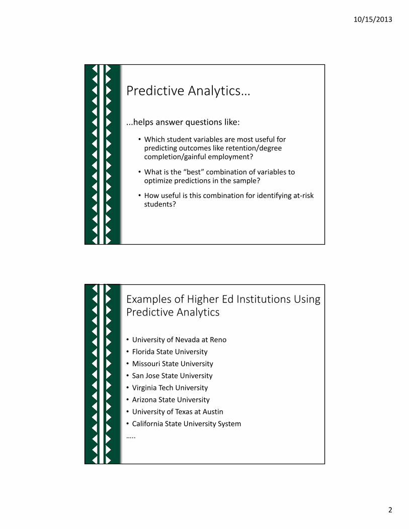
Predictive Analytics…

...helps answer questions like:

• Which student variables are most useful for predicting outcomes like retention/degree completion/gainful employment?

• What is the “best” combination of variables to optimize predictions in the sample?

• How useful is this combination for identifying at‐risk students?

Examples of Higher Ed Institutions Using Predictive Analytics

• University of Nevada at Reno

• Florida State University

• Missouri State University

• San Jose State University

• Virginia Tech University

• Arizona State University

• University of Texas at Austin

• California State University System

…..

10/15/2013

3

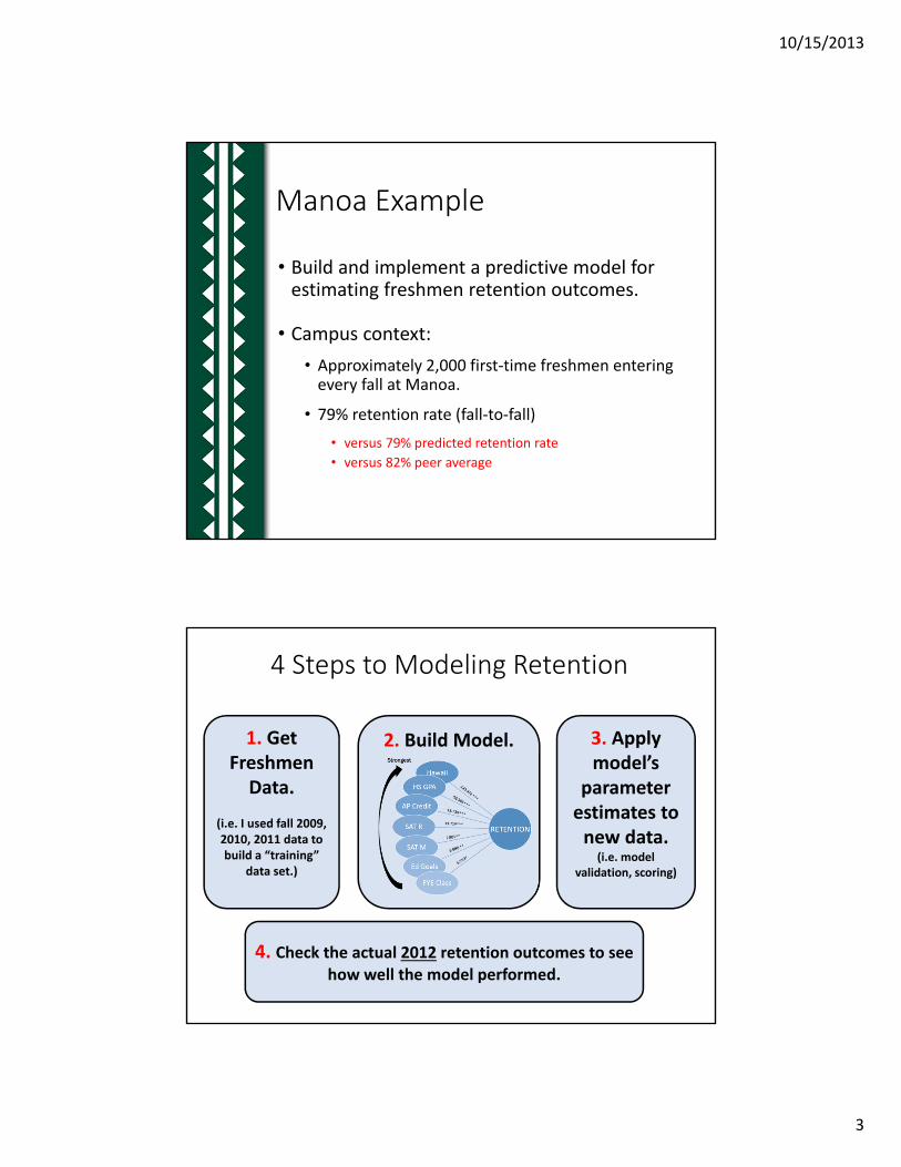
UH Manoa Example

• Build and implement a predictive model for estimating freshmen retention outcomes.

• Campus context:

• Approximately 2,000 first‐time freshmen entering every fall at Manoa.

• 79% retention rate (fall‐to‐fall)

• versus 79% predicted retention rate

• versus 82% peer average

4 Steps to Modeling Retention

1. Get Freshmen Data.

(i.e. I used fall 2009, 2010, 2011 data to build a “training” 

data set.)

4. Check the actual 2012 retention outcomes to see how well the model performed.

2. Build Model. 3. Apply model’s 

parameter estimates to new data.

(i.e. model validation, scoring)

10/15/2013

4

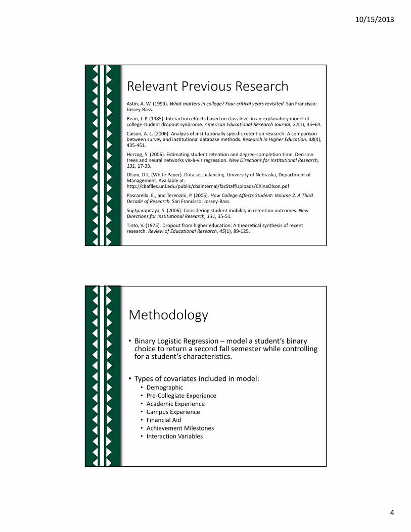
Relevant Previous ResearchAstin, A. W. (1993). What matters in college? Four critical years revisited. San Francisco: Jossey‐Bass.

Bean, J. P. (1985). Interaction effects based on class level in an explanatory model of college student dropout syndrome. American Educational Research Journal, 22(1), 35–64.

Caison, A. L. (2006). Analysis of institutionally specific retention research: A comparison between survey and institutional database methods. Research in Higher Education, 48(4), 435‐451.

Herzog, S. (2006). Estimating student retention and degree‐completion time. Decision trees and neural networks vis‐à‐vis regression. New Directions for Institutional Research,131, 17‐33.

Olson, D.L. (White Paper). Data set balancing. University of Nebraska, Department of Management. Available at: http://cbafiles.unl.edu/public/cbainternal/facStaffUploads/ChinaOlson.pdf

Pascarella, E., and Terenzini, P. (2005). How College Affects Student: Volume 2, A Third Decade of Research. San Francisco: Jossey‐Bass.

Sujitparapitaya, S. (2006). Considering student mobility in retention outcomes. New Directions for Institutional Research, 131, 35‐51.

Tinto, V. (1975). Dropout from higher education: A theoretical synthesis of recent research. Review of Educational Research, 45(1), 89‐125.

Methodology

• Binary Logistic Regression – model a student’s binary choice to return a second fall semester while controlling for a student’s characteristics.

• Types of covariates included in model:• Demographic• Pre‐Collegiate Experience• Academic Experience• Campus Experience• Financial Aid• Achievement Milestones• Interaction Variables

10/15/2013

5

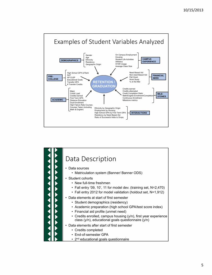
Examples of Student Variables Analyzed

GenderAgeEthnicityResidencyGeographic Origin

High School GPA & RankSATAP CLEPEducational GoalsTransfer GPA# Transfer Credits

MajorCredit LoadCredits Earned First Term GPADistance EducationDual EnrollmentHigh Failure Rate CoursesCourses Taken (including Math & English)

On Campus EmploymentHousingStudent Life ActivitiesAthleticsSTAR UsageAverage Class Size

Need Based AidNon-need Based AidPell GrantWork Study% of Aid Met

Ethnicity by Geographic OriginEmployment by HousingHigh School GPA by First Term GPAResidency by Need Based AidRatio of Successful Adds to Drops

RETENTION / GRADUATION

DEMOGRAPHICS

ACADEMIC

CAMPUS EXPERIENCE

FINANCIAL NEED

INTERACTIONS

Credits earnedCredits attemptedCredit Completion RatioMath/English Enrollment/CompletionContinuous EnrollmentMilestone metrics

MILE-STONES

PRE-COLLEGE

Data Description• Data sources

• Matriculation system (Banner/ Banner ODS)

• Student cohorts• New full-time freshmen• Fall entry ’09, 10’, 11 for model dev. (training set, N=2,470)• Fall entry 2012 for model validation (holdout set, N=1,912)

• Data elements at start of first semester• Student demographics (residency)• Academic preparation (high school GPA/test score index)• Financial aid profile (unmet need)• Credits enrolled, campus housing (y/n), first year experience

class (y/n), educational goals questionnaire (y/n)

• Data elements after start of first semester• Credits completed• End-of-semester GPA• 2nd educational goals questionnaire

10/15/2013

6

• Exploratory data analysis– Variable selection (bivariate regression on outcome

variable)– Variable coding (continuous/categorical/dummy in logit

model)– Missing data imputation, constant-$ conversion (fin. aid

data)– Composite variable(s) – not used in today’s model

• Acad prep index = (HSGPA*12.5)+(ACTM*.69)+(ACTE*.69)– Variables excluded: age, gender, ethnicty, college

remediation, ACT/SAT test date• Logistic regression model

– Maximize model fit (-2LL test/score, pseudo R2, HL sig.)– Create balanced sample in training dataset to optimize

correct classification rate (CCR) for enrollees vs. non-enrollees (i.e. model sensitivity vs. specificity): all non-enrollees plus random sample of enrollees of ~ equal N)

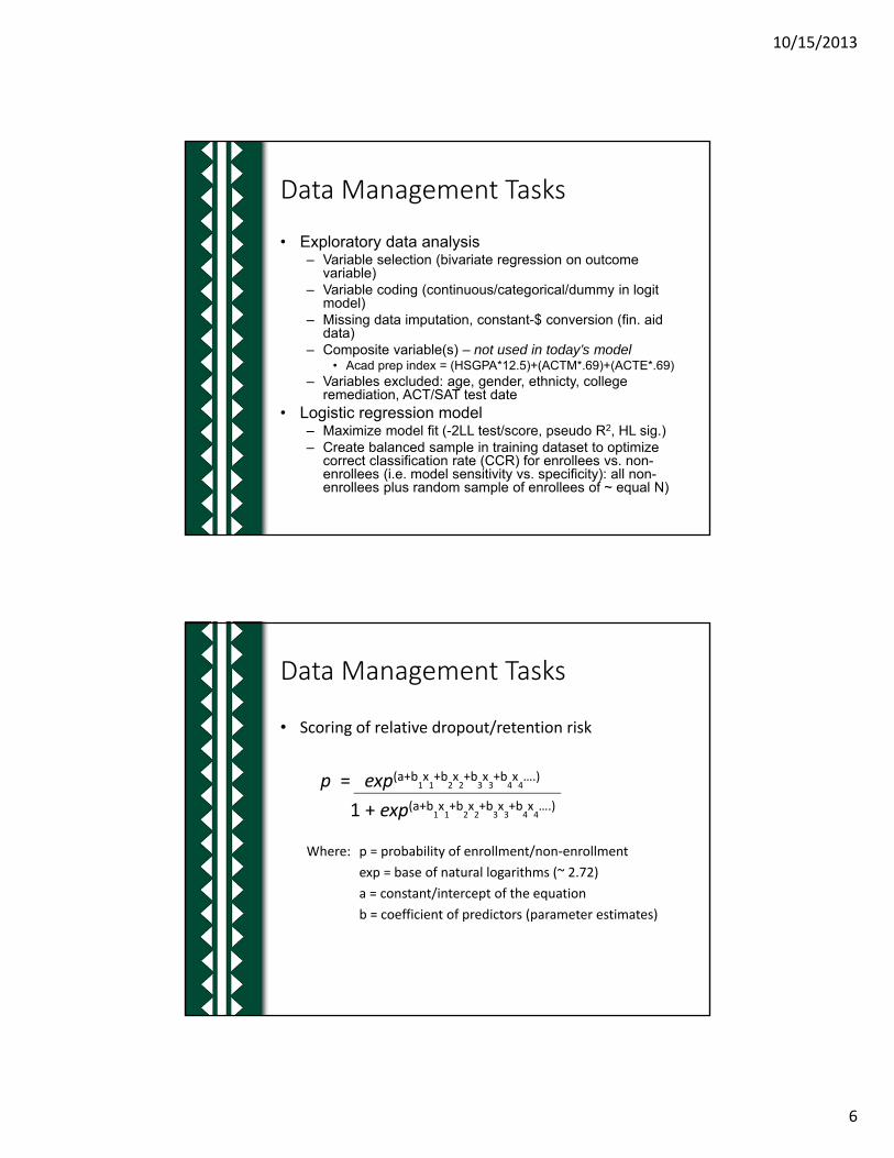
Data Management Tasks

• Scoring of relative dropout/retention risk

p  =   exp(a+b1x1+b2x2+b3x3+b4x4….)

1 + exp(a+b1x1+b2x2+b3x3+b4x4….)

Where: p = probability of enrollment/non‐enrollment

exp = base of natural logarithms (~ 2.72)

a = constant/intercept of the equation

b = coefficient of predictors (parameter estimates)

Data Management Tasks

10/15/2013

7

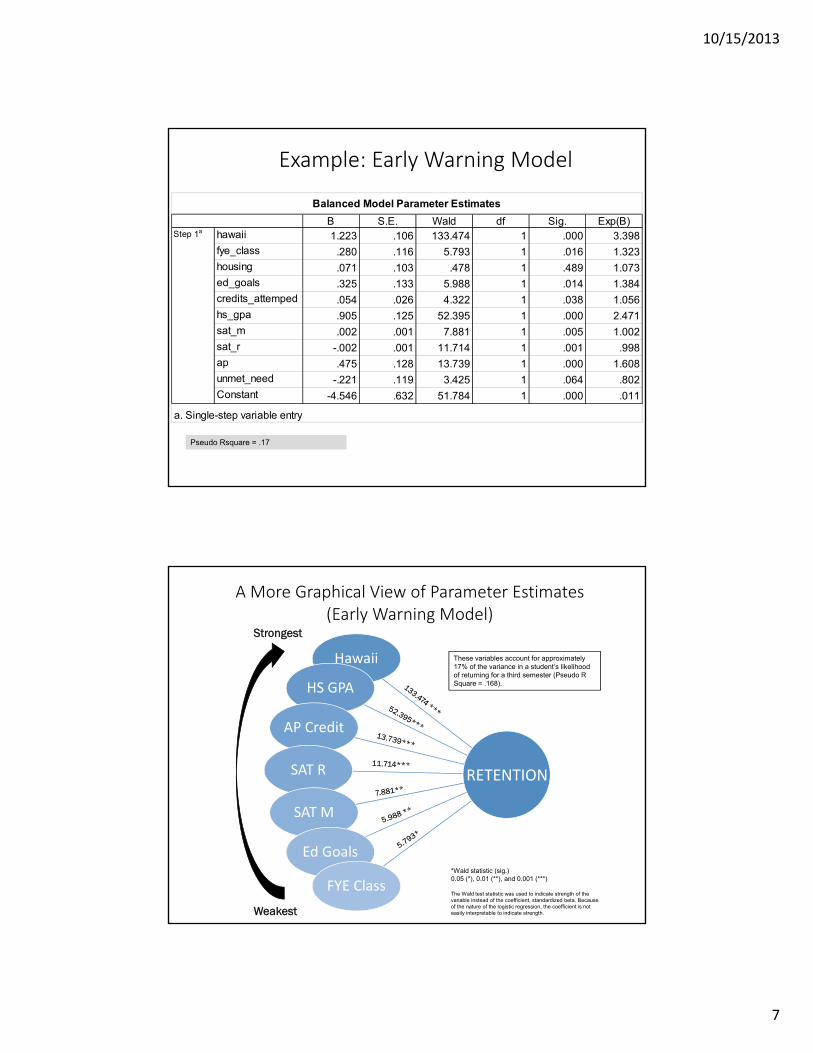
B S.E. Wald df Sig. Exp(B)hawaii 1.223 .106 133.474 1 .000 3.398fye_class .280 .116 5.793 1 .016 1.323housing .071 .103 .478 1 .489 1.073ed_goals .325 .133 5.988 1 .014 1.384credits_attemped .054 .026 4.322 1 .038 1.056hs_gpa .905 .125 52.395 1 .000 2.471sat_m .002 .001 7.881 1 .005 1.002sat_r -.002 .001 11.714 1 .001 .998ap .475 .128 13.739 1 .000 1.608unmet_need -.221 .119 3.425 1 .064 .802Constant -4.546 .632 51.784 1 .000 .011

Balanced Model Parameter Estimates

Step 1a

a. Single-step variable entry

Pseudo Rsquare = .17

Example: Early Warning Model

Strongest

Weakest

*Wald statistic (sig.)0.05 (*), 0.01 (**), and 0.001 (***)

The Wald test statistic was used to indicate strength of the variable instead of the coefficient, standardized beta. Because of the nature of the logistic regression, the coefficient is not easily interpretable to indicate strength.

A More Graphical View of Parameter Estimates (Early Warning Model)

Hawaii

HS GPA

AP Credit

SAT R

SAT M

Ed Goals

FYE Class

These variables account for approximately 17% of the variance in a student’s likelihood of returning for a third semester (Pseudo R Square = .168).

RETENTION

10/15/2013

8

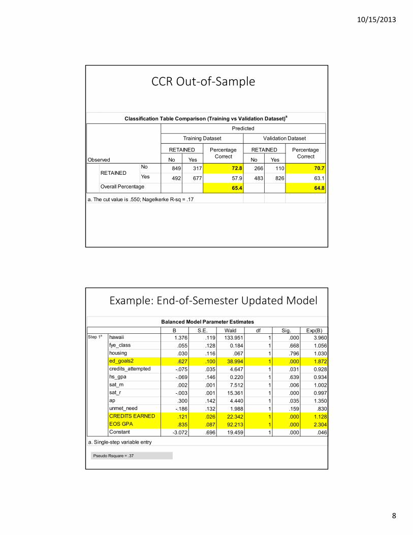
CCR Out‐of‐Sample

No Yes No YesNo 849 317 72.8 266 110 70.7

Yes 492 677 57.9 483 826 63.1

65.4 64.8

RETAINED

Overall Percentage

a. The cut value is .550; Nagelkerke R-sq = .17

Classification Table Comparison (Training vs Validation Dataset)a

Observed

Predicted

Training Dataset Validation Dataset

RETAINED Percentage Correct

RETAINED Percentage Correct

Example: End‐of‐Semester Updated Model

Pseudo Rsquare = .37

B S.E. Wald df Sig. Exp(B)hawaii 1.376 .119 133.951 1 .000 3.960fye_class .055 .128 0.184 1 .668 1.056housing .030 .116 .067 1 .796 1.030ed_goals2 .627 .100 38.994 1 .000 1.872credits_attempted -.075 .035 4.647 1 .031 0.928hs_gpa -.069 .146 0.220 1 .639 0.934sat_m .002 .001 7.512 1 .006 1.002sat_r -.003 .001 15.361 1 .000 0.997ap .300 .142 4.440 1 .035 1.350unmet_need -.186 .132 1.988 1 .159 .830CREDITS EARNED .121 .026 22.342 1 .000 1.128EOS GPA .835 .087 92.213 1 .000 2.304Constant -3.072 .696 19.459 1 .000 .046

Balanced Model Parameter Estimates

Step 1a

a. Single-step variable entry

10/15/2013

9

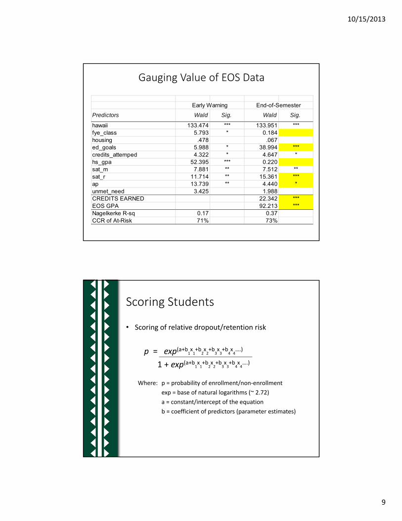
Gauging Value of EOS Data

Predictors Wald Sig. Wald Sig.

hawaii 133.474 *** 133.951 ***fye_class 5.793 * 0.184housing .478 .067ed_goals 5.988 * 38.994 ***credits_attemped 4.322 * 4.647 *hs_gpa 52.395 *** 0.220sat_m 7.881 ** 7.512 **sat_r 11.714 ** 15.361 ***ap 13.739 ** 4.440 *unmet_need 3.425 1.988CREDITS EARNED 22.342 ***EOS GPA 92.213 ***Nagelkerke R-sq 0.17 0.37CCR of At-Risk 71% 73%

Early Warning End-of-Semester

• Scoring of relative dropout/retention risk

p  =   exp(a+b1x1+b2x2+b3x3+b4x4….)

1 + exp(a+b1x1+b2x2+b3x3+b4x4….)

Where: p = probability of enrollment/non‐enrollment

exp = base of natural logarithms (~ 2.72)

a = constant/intercept of the equation

b = coefficient of predictors (parameter estimates)

Scoring Students

10/15/2013

10

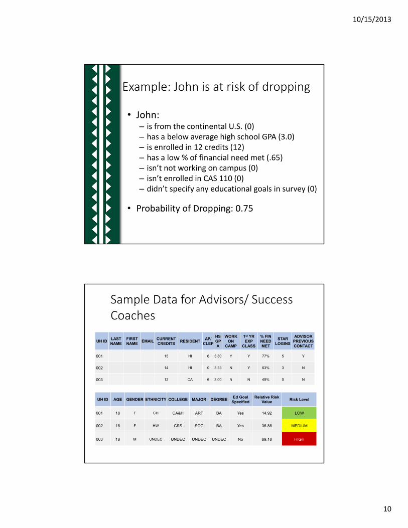
• John: – is from the continental U.S. (0)– has a below average high school GPA (3.0)– is enrolled in 12 credits (12)– has a low % of financial need met (.65)– isn’t not working on campus (0)– isn’t enrolled in CAS 110 (0)– didn’t specify any educational goals in survey (0)

• Probability of Dropping: 0.75

Example: John is at risk of dropping

Sample Data for Advisors/ Success Coaches

UH ID AGE GENDER ETHNICITY COLLEGE MAJOR DEGREEEd Goal

SpecifiedRelative Risk

ValueRisk Level

001 18 F CH CA&H ART BA Yes 14.92 LOW

002 18 F HW CSS SOC BA Yes 36.88 MEDIUM

003 18 M UNDEC UNDEC UNDEC UNDEC No 89.18 HIGH

UH IDLAST NAME

FIRST NAME

EMAILCURRENT CREDITS

RESIDENTAP/

CLEP

HS GPA

WORK ON

CAMP

1st YR EXP

CLASS

% FIN NEED MET

STAR LOGINS

ADVISOR PREVIOUS CONTACT

001 15 HI 6 3.80 Y Y 77% 5 Y

002 14 HI 0 3.33 N Y 63% 3 N

003 12 CA 6 3.00 N N 45% 0 N

10/15/2013

11

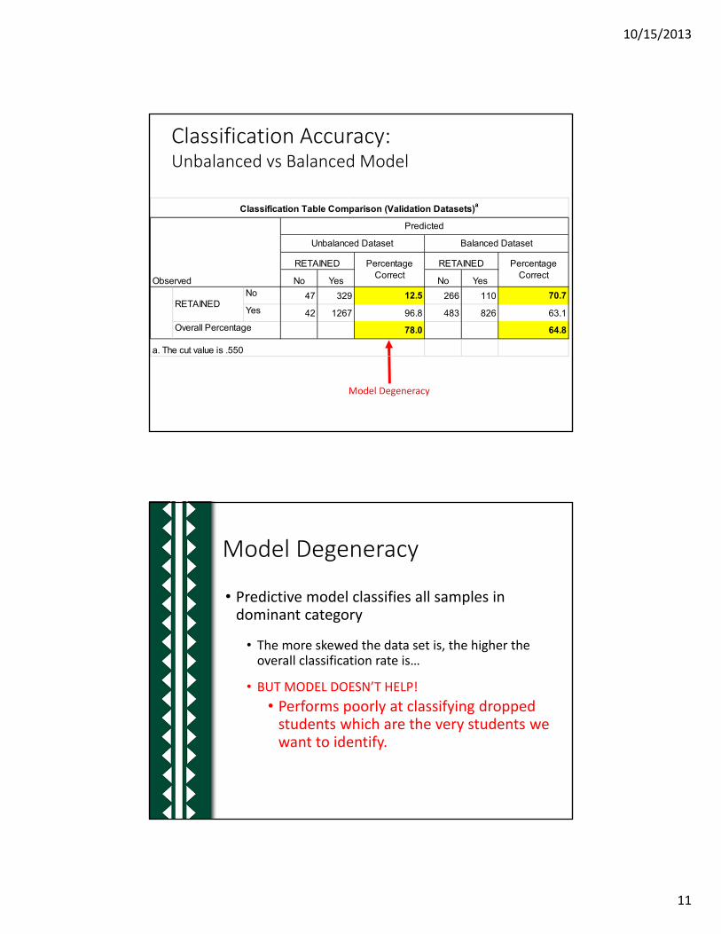
Model Degeneracy

No Yes No YesNo 47 329 12.5 266 110 70.7

Yes 42 1267 96.8 483 826 63.1

78.0 64.8

RETAINED

Overall Percentage

a. The cut value is .550

Observed

Unbalanced Dataset

RETAINED Percentage Correct

Predicted

Balanced Dataset

RETAINED Percentage Correct

Classification Table Comparison (Validation Datasets)a

Classification Accuracy: Unbalanced vs Balanced Model

Model Degeneracy

• Predictive model classifies all samples in dominant category

• The more skewed the data set is, the higher the overall classification rate is…

• BUT MODEL DOESN’T HELP!

• Performs poorly at classifying dropped students which are the very students we want to identify.

10/15/2013

12

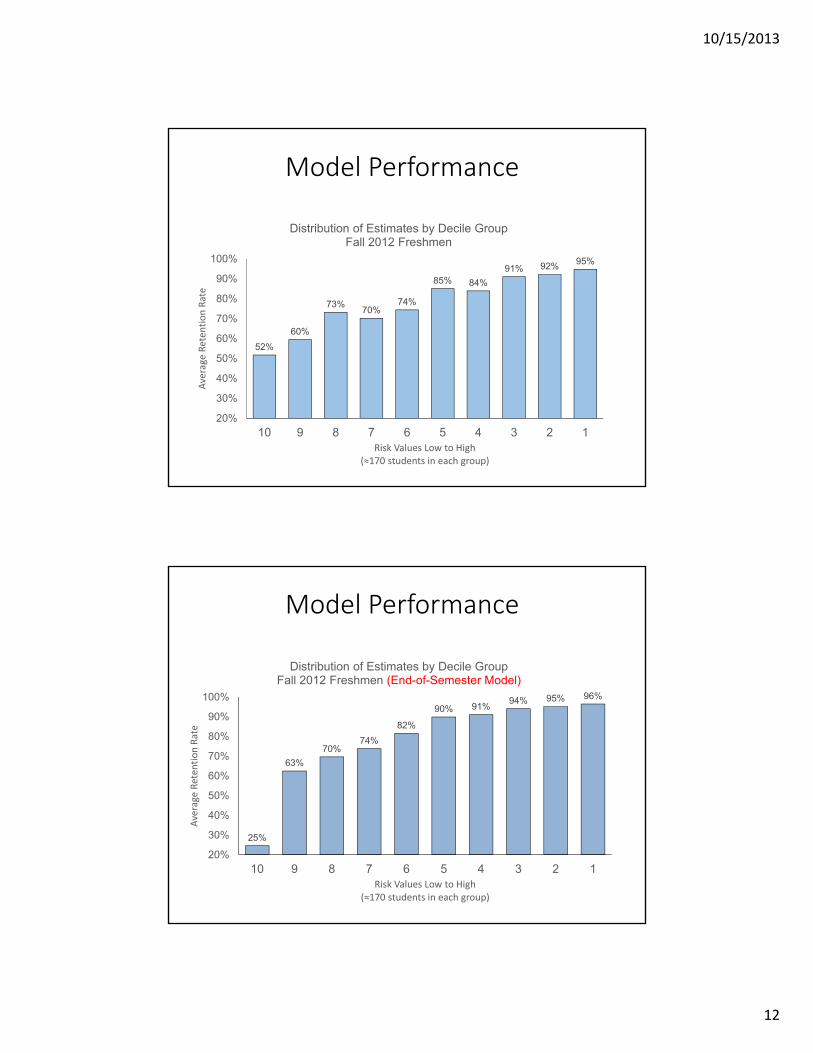
Model Performance

52%

60%

73%70%

74%

85% 84%

91% 92% 95%

20%

30%

40%

50%

60%

70%

80%

90%

100%

10 9 8 7 6 5 4 3 2 1

Average Reten

tion Rate

Risk Values Low to High(≈170 students in each group)

Distribution of Estimates by Decile GroupFall 2012 Freshmen

Model Performance

25%

63%

70%74%

82%

90% 91%94% 95% 96%

20%

30%

40%

50%

60%

70%

80%

90%

100%

10 9 8 7 6 5 4 3 2 1

Average Reten

tion Rate

Risk Values Low to High(≈170 students in each group)

Distribution of Estimates by Decile GroupFall 2012 Freshmen (End-of-Semester Model)

10/15/2013

13

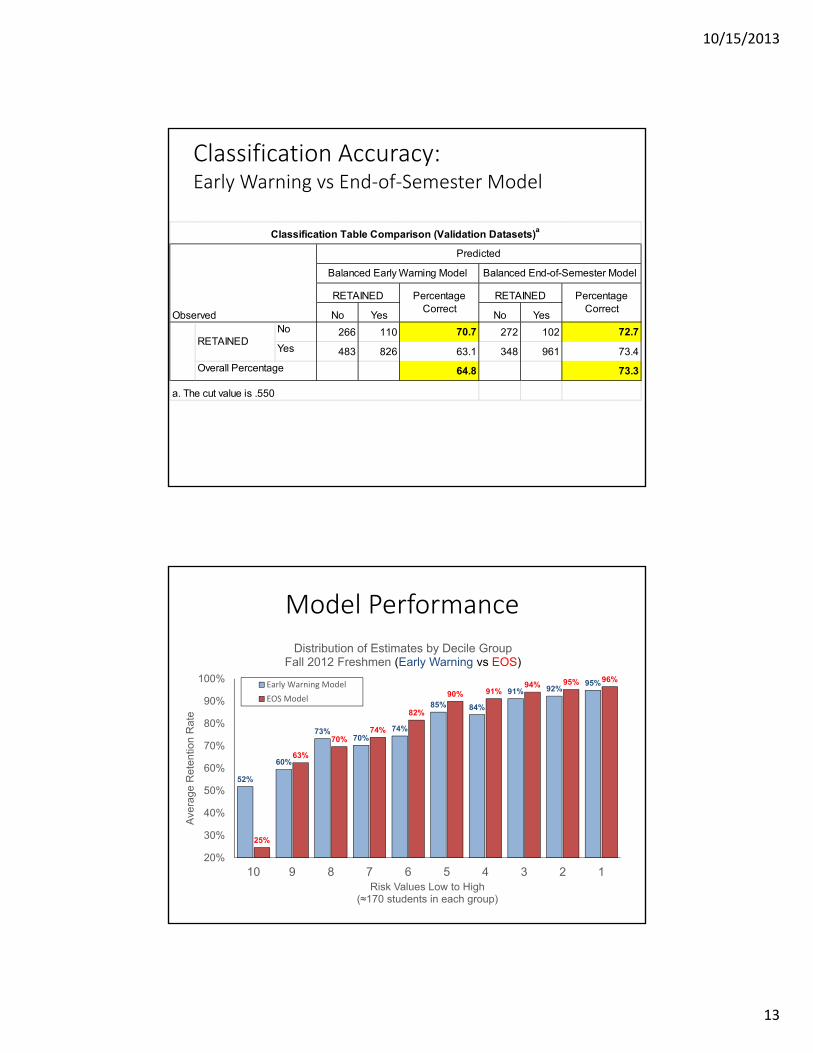
Classification Accuracy: Early Warning vs End‐of‐Semester Model

No Yes No YesNo 266 110 70.7 272 102 72.7

Yes 483 826 63.1 348 961 73.4

64.8 73.3

RETAINED

Overall Percentage

a. The cut value is .550

Predicted

Classification Table Comparison (Validation Datasets)a

Observed

Balanced Early Warning Model Balanced End-of-Semester Model

RETAINED Percentage Correct

RETAINED Percentage Correct

Model Performance

52%

60%

73%70%

74%

85% 84%

91% 92%95%

25%

63%

70%74%

82%

90% 91%94% 95% 96%

20%

30%

40%

50%

60%

70%

80%

90%

100%

10 9 8 7 6 5 4 3 2 1

Ave

rage

Ret

entio

n R

ate

Risk Values Low to High(≈170 students in each group)

Distribution of Estimates by Decile GroupFall 2012 Freshmen (Early Warning vs EOS)

Early Warning Model

EOS Model

10/15/2013

14

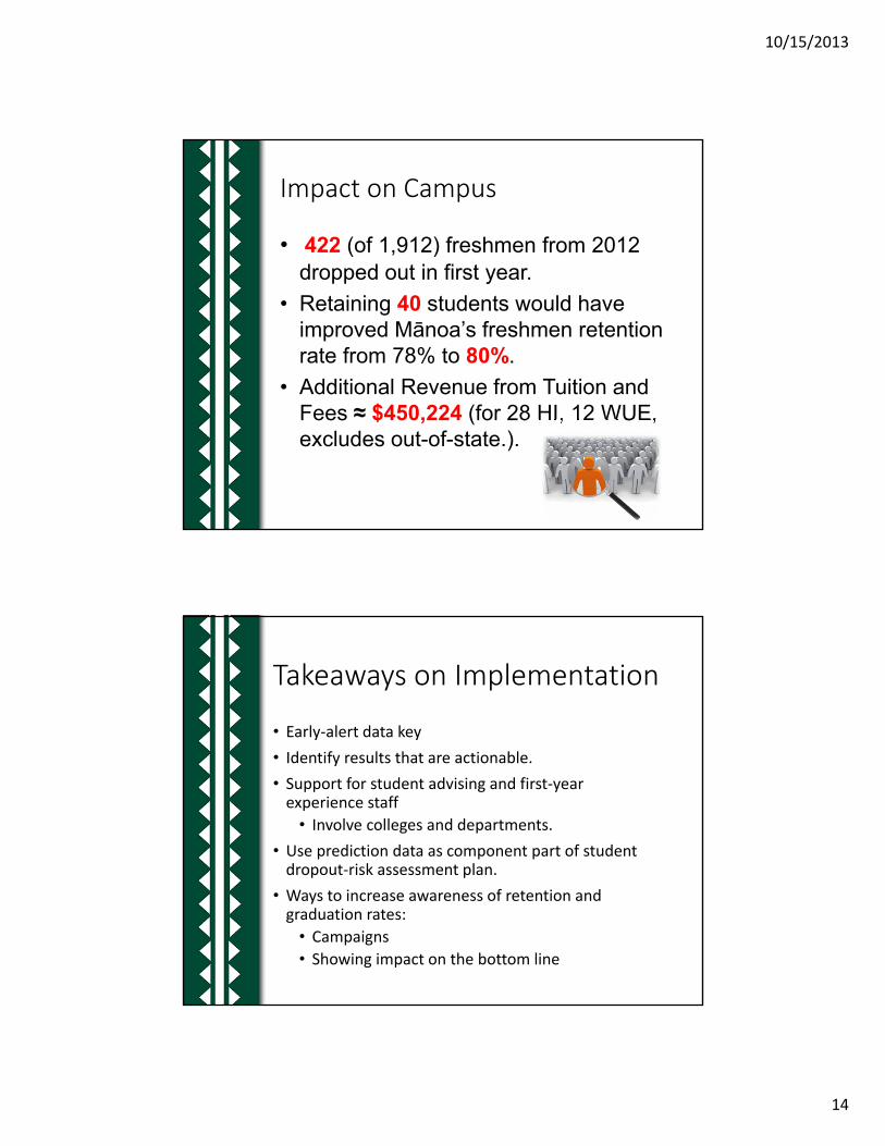
• 422 (of 1,912) freshmen from 2012 dropped out in first year.

• Retaining 40 students would have improved Mānoa’s freshmen retention rate from 78% to 80%.

• Additional Revenue from Tuition and Fees ≈ $450,224 (for 28 HI, 12 WUE, excludes out-of-state.).

Impact on Campus

Takeaways on Implementation

• Early‐alert data key

• Identify results that are actionable.

• Support for student advising and first‐year experience staff

• Involve colleges and departments.

• Use prediction data as component part of student dropout‐risk assessment plan.

• Ways to increase awareness of retention and graduation rates:

• Campaigns

• Showing impact on the bottom line

10/15/2013

15

Challenges to Implementation

• Culture change

• Wary of misuse of data

• Questions about data used in model to generate risk scores

• Students’ rights to access risk scores

• More accountability

• Faculty buy‐in

Summary• Predicting students at‐risk

• Keep prediction model parsimonious• Keep prediction data for student advising intuitive and simple (actionable)

• Triangulate prediction data with multiple sources of information• Use prediction data as component part of student dropout‐risk assessment

• Follow ‘best practices’ in predictive analytics and keep abreast of changes in analytical and data reporting tools

• Using prediction data• Embrace the use of available data• Ensure users conceptually understand what’s behind the data• Use data as a complementary piece of information when advising students

• Timing can be critical in terms of student intervention as well as maximizing advising resources

• Stay abreast of new research on predictive analytics: • E.g. “Analytics in Higher Education” by J. Bichsel, Educause, 2012

10/15/2013

16

John StanleyInstitutional Analyst

University of Hawaii at Manoa

Questions: jstanley@hawaii.edu

Link to this presentation:

http://manoa.hawaii.edu/ovcaa/mir/pdf/datasummit2013.pdf

Mahalo