What is it?SeaBED is an Autonomous Underwater

Vehicle (AUV) built under the sponsorship of

the Office of Naval Research, and the

National Science Foundation’s Censsis

Engineering Research Center.

The SeaBED AUVThe objective of the Seabed AUV is to serve as a readily available and operationally simple tool that allows rapidtesting of docking methodologies and imaging algorithms. We expect to actively pursue repeat surveys for changedetection and quantification in areas such as: sidescan sonar survey, photomosaicking, 3D image reconstructionfrom a single camera, image based navigation, and multi-sensor fusion of acoustic and optical data.

Seabed is a hover-capable vehicle that performs optical sensing with a 12bit 1280x1024 monochrome CCD cam-era. Acoustic high resolution mapping is achieved using an MST 300 kHz sidescan sonar with a swath width of 400m. A Seabird conductivity and temperature sensor, RDI ADCP and Acoustic Modem are also present.

The AUV is designed for operations from small vessels with minimal support equipment. It has an operational depthof 2000 meters and at 1 m/s can run for up to 10 hours and survey 36 km per mission.

Navigation is performed with standard long baseline (LBL) acoustic nets and a Doppler Velocity Log (DVL), whichalso performs water column current measurements. Update rates are in the order of 5 Hz, allowing closed loopcontrol of position. Depth is measured from a Paroscientific pressure sensor while altitude is obtained from theDVL. A Crossbow AHRS provides heading, pitch and roll readings. Current capabilities allow positioning accuracyon the order of 0.1 meters.

Why is it different and what have weaccomplished?From the start our goals were to design a small, but capable, AUV for imaging research and long term untendeddeployments in shallow water and the deep ocean.

Based on our design constraints some of the highlights of SeaBEDinclude• A mechanical design that is hover capable, and passively stable in pitch and roll. This makes it ideally suited for

imaging applications such as sidescan sonar surveys, bathymetric surveys and video transects.

• Our thrusters use permanent magnets for coupling thereby bypassing the shaft seal problem. Moreover, wemade a conscious decision not to use oil-filled thrusters so that we did not have to worry compensation oilvolumes over deployments lasting months.

• Our software uses standard C and Perl and runs on a PC-104 (Pentium 133 MHz with 64 Meg RAM) systemwith Redhat Linux version 6.2. We felt that we could easily achieve soft real-time performance under this oper-ating paradigm. We are currently running our control cycle at 10Hz with 20%-30% CPU utilization, i.e. have noreal concerns about current or future computational requirements.

What we have under our belts• We have an extremely reliable AUV (at least so far - we haven’t opened the electronics or battery housing in weeks!).

• We have demonstrated sidescan sonar (from Marine Sonics Technologies) deployments in shallow water inboth altitude following and constant depth mode, with transducers that are rated to full ocean depth (see ourinteresting story about finding a “wreck” in Buzzards’ Bay :-).

• We have demonstrated several missions that were hour long and beyond and see no problems with running tenhour missions associated with full battery capacity.

• We have completed seven (so far), sealed charge / discharge cycles of our Lithium Ion battery chemistry in asealed pressure vessel.

• We have demonstrated missions in very high current environments - we worked off of Muskeget Channel off ofVineyard Sound where the current was flowing at 3-4 knots. We decided to simply fly with the current whileholding heading and depth.

• We have demonstrated very precise navigation, trackline following, using our RD Instruments ADCP (see Figure1 below for an example).

• We can operate the entire vehicle with one person (of course two people means that we can check up on eachother) off of very small platforms such as the 40 foot R/V Asterias.

Here’s data from an example mission

The first “wreck” wediscovered...One of our initial sidescan sonar missions was in Buz-zards Bay where the bottom is flat mud with very fewfeatures. So we ran a mission and imagine our surprisewhen we saw this beautiful outline of a boat on thebottom (Figure 4) We had great nav and always knewwe could go back to it but I was more concerned aboutevaluating our sonar performance so we trundled off tothe Wee Peckets and ran a couple of missions there.Figures 1 through 3 were from one of the missions weran there. That night while reviewing all our navigationand sonar data I found

• That the time associated with finding the wreck wasright at the end of our mission when the vehicle wasdrifting on the surface.

• Also, we found what looked like the same boat (Fig-ure 5) at the very end of one of our Wee Pecket mis-sions. That it too turned up right at the end of ourmission, and more interestingly it had a wake associ-ated with it ;-), really got me thinking.

• Quick calculations showed we were imaging ourselves (the R/V Asterias!). While a sidescan sonar usually as-sumes that the ground is fixed and the towfish is moving, in this case we had a stationary fish, flat calm waters.

• (i.e. ideal conditions for surface reflections) and a moving object on the surface!!! The good news - our sidescan sonar has very good sensitivity.

What’s next...In March we’ve teamed up with our ERC partners Luis Jiminez and Fernando Gilbes at the University of Puerto Ricoat Mayagüez in a joint project aimed at the long term health assessment of coral reefs. We’ll be making yearly visitsto a coral reef site and constructing color photomosaics from the unstructured imagery collected with our 12-bitCCD camera. Temporal change detection and repeatable surveys will be key aspects of the problem.

In addition we will have a very full year next year with deployments off of Martha’s Vineyard to look at MCM andin the fall we’ll be teaming up with the University of Concepcion in Chile in a biological application to assess thehealth of lobster populations off the coast of Chile.

Acknowledgements:The vehicle core team is composed of Hanumant Singh, Ryan Eustice, Christopher Roman, Oscar Pizarro andNeil McPhee.

Steve Lerner, John Laplante, Frank Weyer, and Eric Gifford, did extremely crucial work at various stages.

We got lots of advice, significant bits of software and hardware, and encouragement from Al Bradley, Dana Yoerger,Rob Sohn, Lee Freitag, Louis Whitcomb, Steve Liberatore, Jack Zhang, and Jonathan Howland.

Contact InformationWe did a number of missions and have a lot of data that could not be packed into this document. I’d be happy toshow you more data and to talk about possible collaborations in the future. Feel free to contact me athanu@whoi.edu.

Table 1: SeaBED Vehicle Characteristics

Vehicle Depth Capability 2000 m

Size 2.0m(L), 1.5m(H),

Mass 200 kg in air

Speed Range (Typical) 0-1.5m/s (1.0m/s)

Batteries 2kWh rechargeable Li-ion Pack

Propulsion Four DC thrustersFore 100NLateral 50NVertical 50N

Navigation and Attitude Attitude & Heading Crossbow AHRSDepth Paroscientific pressure sensor, 0.01%Position LBL+ 300 kHz RDI navigator, 0.1-1 mAltitude RDI navigator, 0.1 m

Optical Imaging Electronic Camera Pixelfly 12bit 1280x1024 bw CCDLighting one 200 Watt-second strobeSeparation 1m from Camera to light

Acoustic Imaging Sidescan sonar MST 300 kHz (300 m depth capability)

Other Sensors CTD Seabird 37SBIADCP 300 kHz RDI navigator

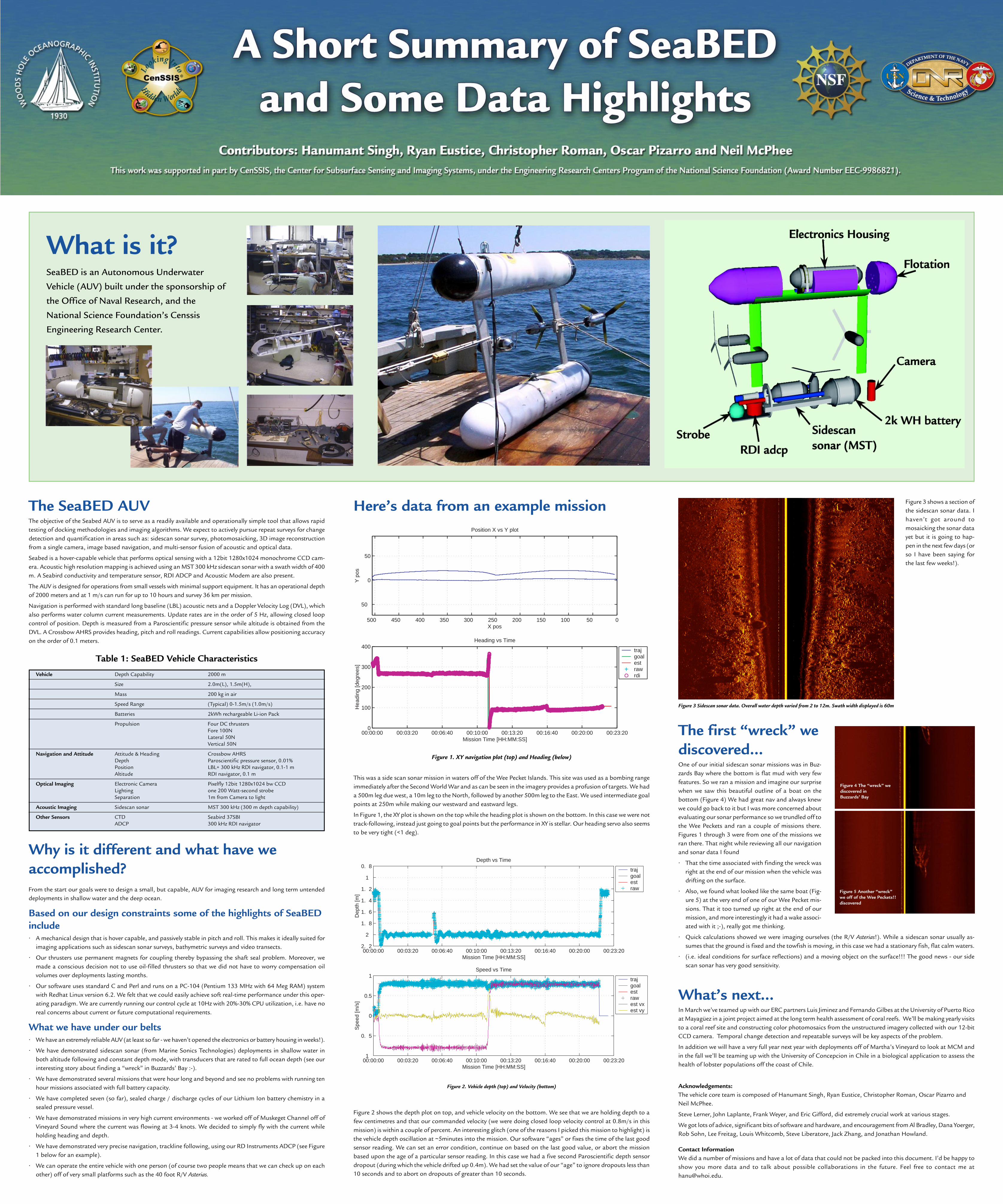
This was a side scan sonar mission in waters off of the Wee Pecket Islands. This site was used as a bombing rangeimmediately after the Second World War and as can be seen in the imagery provides a profusion of targets. We hada 500m leg due west, a 10m leg to the North, followed by another 500m leg to the East. We used intermediate goalpoints at 250m while making our westward and eastward legs.

In Figure 1, the XY plot is shown on the top while the heading plot is shown on the bottom. In this case we were nottrack-following, instead just going to goal points but the performance in XY is stellar. Our heading servo also seemsto be very tight (<1 deg).

Figure 2 shows the depth plot on top, and vehicle velocity on the bottom. We see that we are holding depth to afew centimetres and that our commanded velocity (we were doing closed loop velocity control at 0.8m/s in thismission) is within a couple of percent. An interesting glitch (one of the reasons I picked this mission to highlight) isthe vehicle depth oscillation at ~5minutes into the mission. Our software “ages” or fixes the time of the last goodsensor reading. We can set an error condition, continue on based on the last good value, or abort the missionbased upon the age of a particular sensor reading. In this case we had a five second Paroscientific depth sensordropout (during which the vehicle drifted up 0.4m). We had set the value of our “age” to ignore dropouts less than10 seconds and to abort on dropouts of greater than 10 seconds.

Figure 3 shows a section ofthe sidescan sonar data. Ihaven’t got around tomosaicking the sonar datayet but it is going to hap-pen in the next few days (orso I have been saying forthe last few weeks!).

Figure 3 Sidescan sonar data. Overall water depth varied from 2 to 12m. Swath width displayed is 60m

trajgoalest raw

traj goal est raw est vxest vy

00:00:00 00:03:20 00:06:40 00:10:00 00:13:20 00:16:40 00:20:00 00:23:201

0. 5

0

0.5

1

Spe

ed [m

/s]

Speed vs Time

Mission Time [HH:MM:SS]

00:00:00 00:03:20 00:06:40 00:10:00 00:13:20 00:16:40 00:20:00 00:23:202. 2

2

1. 8

1. 6

1. 4

1. 2

1

0. 8Depth vs Time

Dep

th [m

]

Mission Time [HH:MM:SS]

Figure 2. Vehicle depth (top) and Velocity (bottom)

trajgoalest raw rdi

00:00:00 00:03:20 00:06:40 00:10:00 00:13:20 00:16:40 00:20:00 00:23:200

100

200

300

400Heading vs Time

Hea

ding

[deg

rees

]

Mission Time [HH:MM:SS]

500 450 400 350 300 250 200 150 100 50 0

50

0

50

Position X vs Y plot

X pos

Y p

os

Figure 1. XY navigation plot (top) and Heading (below)

Figure 4 The “wreck” wediscovered inBuzzards’ Bay

Figure 5 Another “wreck”we off of the Wee Peckets!!discovered