What is behind the rise in long-term unemployment?;/media/publications/...What is behind the rise in long-term unemployment? Daniel Aaronson, Bhashkar Mazumder, and Shani Schechter

28 2Q/2010, Economic Perspectives

What is behind the rise in long-term unemployment?

Daniel Aaronson, Bhashkar Mazumder, and Shani Schechter

Daniel Aaronson is a vice president and economic advisor in the Economic Research Department at the Federal Reserve Bank of Chicago. Bhashkar Mazumder is a senior economist in the Economic Research Department and the executive director of the Chicago Census Research Data Center at the Federal Reserve Bank of Chicago. Shani Schechter is an associate economist in the Economic Research Department at the Federal Reserve Bank of Chicago. The authors thank Lisa Barrow, Bruce Meyer, and Dan Sullivan for helpful comments and Constantine Yannelis for excellent research assistance.

Introduction and summary

As we entered 2010, the average length of an ongoing spell of unemployment in the United States was more than 30 weeks—the longest recorded in the post-World War II era. Remarkably, more than 4 percent of the labor force (that is, over 40 percent of those unemployed) were out of work for more than 26 weeks—we consider these workers to be long-term unemployed. In contrast, the last time unemployment reached 10 percent in the United States, in the early 1980s, the share of the labor force that was long-term unemployed peaked at 2.6 per-cent. Although there has been a secular rise in long-term unemployment over the last few decades, the sharp increases that occurred during 2009 appear to be out-side of historical norms. Further, this trend may present important implications for the aggregate economy and for macroeconomic policy going forward.

The private cost of losing a job can be sizable. In the short run, lost income is only partly offset by unemployment insurance (UI), making it difficult for some households to manage their financial obligations during spells of unemployment (Gruber, 1997; and Chetty, 2008). In the long run, permanent earnings losses can be large, particularly for those workers who have invested time and resources in acquiring knowledge and skills that are specific to their old job or industry (Jacobson, LaLonde, and Sullivan, 1993; Neal, 1995; Fallick, 1996; and Couch and Placzek, 2010). Health consequences can be severe (Sullivan and von Wachter, 2009). Research even suggests that job loss can lead to negative outcomes among the children of the unemployed (Oreopoulos, Page, and Stevens, 2008) and to an increase in crime (Fougère, Kramarz, and Pouget, 2009).

All of these costs are likely exacerbated as un-employment spells lengthen. The probability of find-ing a job declines as the length of unemployment increases. Although there is some debate as to exactly

what this association reflects, it is certainly plausible that when individuals are out of work longer, their labor market prospects are diminished through lost job skills, depleted job networks, or stigma associated with a long spell of unemployment (Blanchard and Diamond, 1994).1 For risk-averse households that can-not insure completely against a fall in consumption as they deplete their precautionary savings, the welfare consequences of job loss rise as unemployment dura-tion increases. Welfare implications are particularly severe during periods of high unemployment for indi-viduals with little wealth (Krusell et al., 2008).

In this article, we analyze the factors behind the recent unprecedented rise in long-term unemployment and explain what this rise might imply for the economy going forward. Using individual-level data from the U.S. Bureau of Labor Statistics’ Current Population Survey (CPS), we show that all of the substantial rise in the average duration of unemployment between the mid-1980s and mid-2000s can be explained by demo-graphic changes in the labor force, namely, the aging of the population and the increased labor force attachment of women (Abraham and Shimer, 2002). But only one-half of the increase in average duration of unemploy-ment at the end of 2009 relative to that of the early 1980s may be due to demographic factors. This suggests that other factors have come into play more recently.

29Federal Reserve Bank of Chicago

In particular, we attribute the sharp increase in unem-ployment duration in 2009 to especially weak labor demand, as reflected in a low rate of transition out of unemployment into employment, and a smaller portion of this increase (perhaps 10 percent to 25 percent) to extensions in unemployment insurance benefits.2

We show that, in any given month, individuals with longer unemployment spells are less likely to be employed the following month. This suggests that the average ongoing spell of unemployment is likely to remain longer than usual well into the economic re-covery and expansion, plausibly keeping the unemploy-ment rate above levels observed in past recoveries. For example, we find that if the current distribution of unemployment duration resembled historical dis-tributions, the unemployment rate would be roughly 0.4 percentage points lower than it is today. Neverthe-less, we find no evidence that high levels of long-term unemployment will have a sizable impact on compen-sation growth going forward.

We begin by presenting some descriptive facts about trends and business cycle movements of unem-ployment duration. We then analyze how much of the increase in the recent average duration of unemploy-ment compared with that of the previous severe reces-sion and its aftermath (in 1982–83) can be explained by changes in the demographic, industrial, and occupa-tional composition of the labor force versus changes in the average duration of unemployment within the various groups. We next consider how much of the remaining increase can be attributed to weak labor demand and extensions of unemployment benefits. Finally, we examine how high levels of long-term unemployment may affect the unemployment rate and compensation growth going forward.

The rise of long-term unemployment

We begin by reviewing some facts about unemploy-ment spell length. Long-run estimates of unemploy-ment duration are available back to the late 1940s from the Current Population Survey, a monthly survey of 60,000 or more households. Respondents are 16 years and older and are asked to classify themselves as em-ployed, unemployed, or out of the labor force. Those unemployed are further asked how long, in weeks, their unemployment has lasted. As a result, the CPS duration measures are based on ongoing spells of unemploy-ment and are not measures of completed spell length.

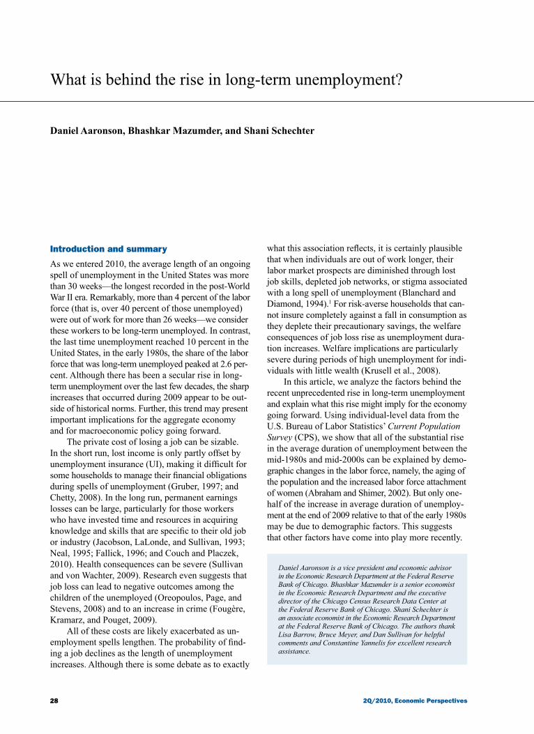
Figure 1 plots the average (and median) duration of unemployment from 1948 (and 1967) through the end of 2009. Over the past half century, the average length of spells of unemployment have increased, from 11.3 weeks in the 1960s to 11.8 weeks in the 1970s,

11.9 weeks in the 1980s, 15.0 weeks in the 1990s, and 17.4 weeks in the 2000s.3 Figure 2 plots the share of the unemployed that are short-term (fewer than five weeks) versus long-term (more than 26 weeks). There has been a pronounced shift over time in the composition of the unemployed by duration, with a particularly sharp change in 2009. Long-term unemployment accounted for 10 percent of the unemployed in the 1950s and 1960s; it reached 26 percent in the early 1980s; and it averaged roughly 20 percent between 2002 and 2007, but reached 40 percent as of December 2009.4 By the end of last year, over 4 percent of the labor force was long-term unemployed.

The average duration of unemployment is counter-cyclical—that is, it increases when the overall econo-my is shrinking, as figure 1 makes clear. Therefore, figure 3, panel A presents a scatter plot of average dura-tion of unemployment against the unemployment rate to provide a simple way of comparing durations con-ditional on the unemployment rate. Each blue or black box represents a month. The black line represents the re-lationship between the unemployment rate and average duration of unemployment over the period 1948–2007. Because the line is upward sloping, it illustrates that worse labor market conditions (higher unemployment rates) are associated with longer unemployment spells. In particular, through 2007, an extra 1 percentage point on the unemployment rate was associated with spells that lasted 1.2 weeks longer on average.

For the most recent period, we use black boxes to represent months between December 2007 (the start of the most recent recession) and December 2009 in figure 3, panel A. Note that all the black boxes lie near the top of the cloud of blue boxes, highlighting that the average unemployment spell tends to be much longer now for any given unemployment rate. As the economy weakened and the unemployment rate rose, the length of unemployment spells increased—and at a pace that was fairly typical for a recession. This is represented by the black boxes that lie roughly parallel to the black line. But, starting in June 2009 (the half dozen or so black boxes on the right side of panel A), unemployment spells began to lengthen to unprecedented levels. Much of this spike in average duration of unemployment is driven by the unmistakable increase in the share of the unem-ployed out of work for more than 26 weeks, highlighted by the black boxes in figure 3, panel B. For instance, the average length of unemployment during the last six months of 2009 was over seven weeks longer than that of the first six months of 1983, when unemploy-ment had peaked at 10.8 percent.

Looking forward, we should expect to see a his-torically long average duration of unemployment for


weeks

Average and median duration of unemployment, 1948–2009FIguRE 1

’53 ’58 ’63 ’68 ’73 ’78 ’83 ’88 ’93 ’98 2003 ’080

5

10

15

20

25

30

Average Median

1948

Note: The shaded areas indicate official periods of recession as identified by the National Bureau of Economic Research; the dashed vertical line indicates the most recent business cycle peak. Source: U.S. Bureau of Labor Statistics, Current Population Survey, from Haver Analytics.

percentage of unemployed

Short-term and long-term share of unemployment, 1948–2009FIguRE 2

Note: The shaded areas indicate official periods of recession as identified by the National Bureau of Economic Research; the dashed vertical line indicates the most recent business cycle peak.Source: U.S. Bureau of Labor Statistics, Current Population Survey, from Haver Analytics.

1948 ’53 ’58 ’63 ’68 ’73 ’78 ’83 ’88 ’93 ’98 2003 ’08

0

10

20

30

40

50

60

70

More than 26 weeks Fewer than five weeks


FIguRE 3

A. Average duration of unemployment versus unemployment rateaverage duration of unemployment in weeks

Unemployment rate, duration of unemployment, and long-term share of unemployment, 1948–2009

B. Long-term share of unemployment versus unemployment rate percentage of the unemployed who are long-term unemployed

Notes: In panel A, the black line represents the relationship between the unemployment rate and average duration of unemployment over the period January 1948–November 2007. In panel B, the black line represents the relationship between the unemployment rate and the share of the unemployed who are more than 26 weeks unemployed over the period January 1948–November 2007.Source: Authors’ calculations based on data from the U.S. Bureau of Labor Statistics, Current Population Survey, from Haver Analytics.

some time, since it is typical for average spell length to rise well past the business cycle trough. This is appar-ent in figure 4, which plots the cyclical pattern in the average duration of unemployment versus the unem-ployment rate for several selected cycles. In both the mid-1970s and the early 1980s (blue lines), average

duration stayed persistently high, even as the unem-ployment rate began to decline.5 As labor demand picks up early in a recovery, employers might turn to unemployed workers with shorter spells first, leaving the unemployment pool increasingly composed of those with relatively longer spells. Sequential hiring

0

5

10

15

20

25

30

35

0 2 4 6 8 10 12unemployment rate

0

5

10

15

20

25

30

35

40

45

0 2 4 6 8 10 12

January 1948–November 2007 December 2007–December 2009

unemployment rate


FIguRE 4

average duration of unemployment in weeks

Unemployment rate versus average duration of unemployment for selected business cycles

Source: U.S. Bureau of Labor Statistics, Current Population Survey, from Haver Analytics.

patterns like this may be due in part to a selection effect: Those who are less employable are the ones who are likely to remain unemployed longer and are less likely to be rehired. However, the lower reemployment probability of the long-term unemployed may also be due to diminished job skills, weakened social networks, and the assumption by some employers of poor worker quality that accompany those with longer spells. De-clines in job separations, which we discuss in more de-tail later, may also reduce the number of short spells of unemployment in the early stages of a recovery.

Unemployment duration versus other labor market measures

It is important to emphasize that the recent spike in the duration of unemployment not only is quite large by historical standards but also stands out relative to the recent deterioration in many other key labor market indi-cators, including three key measures used to gauge labor market slack: the unemployment rate, a broader unem-ployment rate (the U.S. Bureau of Labor Statistics’ U-6 rate),6 and total payroll employment. That observation can best be seen from a very simple statistical model that uses gross domestic product (GDP) growth to generate out-of-sample forecasts of these labor market

measures. This exercise when applied to the unem-ployment rate is the basis for what is often referred to as “Okun’s law.”7 We follow Aaronson, Brave and Schechter (2009) and use two samples to estimate these relationships: 1) all data from the first quarter of 1978 through the second quarter of 2007 and 2) data solely from the recessions during that period.

Figure 5 shows the results for four measures of the labor market—namely, the unemployment rate, the U-6 rate, total payroll employment, and the average duration of unemployment. Each panel of figure 5 con-tains three colored lines. The blue line represents the actual data, the black line is the forecast based on the data from our full sample, and the gray line is the forecast based on only recession periods in the full sample. Note that the recession sample forecasts use the recession-period coefficients to forecast through the end of 2009, even though the recession likely ended earlier.

Across all the measures in figure 5, the forecasts based on the full sample of data consistently under-predict the deterioration in labor market conditions. For example, the unemployment rate forecasted (panel A) at the end of 2009 lies roughly 2 percentage points below the actual unemployment rate, a finding noted by many commentators who worry that Okun’s law no

December 2007–December 2009

July 1981–December 1983

December 1973–November 1976

unemployment rate

0

5

10

15

20

25

30

35

0 2 4 6 8 10 12


longer applies and labor markets are not functioning as in the past. However, if we use the recession sample (gray line), this simple activity model does a remarkably good job at forecasting the cumulative rise in the stan-dard (panel A) and broader (panel B) unemployment rates and the fall in total payroll employment (panel C). That is, labor markets have mostly evolved about as we would expect given the severity of the recession.

But such a conclusion is not warranted for unem-ployment duration (panel D of figure 5).8 Forecasts based on both the full and recession samples fail to predict by up to over a month the dramatic rise in that series, starting in the fourth quarter of 2008. The remainder of this article is therefore focused on explaining the causes of the strikingly unusual increase in the length of unemployment spells.

Who are the long-term unemployed and how have they changed over time?

Figure 3 (p. 31) highlights the spike in average unemployment duration and long-term unemployment in 2009. It also illustrates that unemployment duration was already historically high going into the recent recession given the unemployment rate at the time. Relative to the black regression line that predicts dura-tion based on the contemporaneous unemployment rate (figure 3, panel A), the black boxes there suggest that unemployment spells were already about four to five weeks higher, on average, than those during 1948–2007. For that reason, at least part of the explanation for current lengths of unemployment happened years ago.

Accordingly, table 1 examines the background char-acteristics of the long-term unemployed, in particular

FIguRE 5

Out-of-sample forecasts of labor market variables, 2007–09

A. Unemployment rate percent

B. U-6 rate percent

C. Total payroll employmentmillions of jobs

D. Average duration of unemploymentweeks

Notes: Each panel is based on a simple statistical model that uses gross domestic product growth to generate out-of-sample forecasts of the labor market measure. All data from the first quarter of 1978 through the second quarter of 2007 are used to estimate the full sample forecasts, while data from just the recessions in this period are used to estimate the recession sample forecasts. The U-6 rate is a broader unemployment rate from the U.S. Bureau of Labor Statistics (see note 6 for details).Sources: Authors’ calculations based on data from the U.S. Bureau of Labor Statistics, Current Population Survey, basic monthly files; and Haver Analytics.

Q2 Q3 Q4 Q1 Q2 Q3 Q4 Q1 Q2 Q3 Q40

2

4

6

8

10

12

0

2

4

6

8

10

12

14

16

18

124

126

128

130

132

134

136

138

140

0

5

10

15

20

25

30

2007 2008 2009Q2 Q3 Q4 Q1 Q2 Q3 Q4 Q1 Q2 Q3 Q4 2007 2008 2009

Q2 Q3 Q4 Q1 Q2 Q3 Q4 Q1 Q2 Q3 Q4 2007 2008 2009

Q2 Q3 Q4 Q1 Q2 Q3 Q4 Q1 Q2 Q3 Q4 2007 2008 2009

Actual Predicted based on full sample Predicted based on recession sample


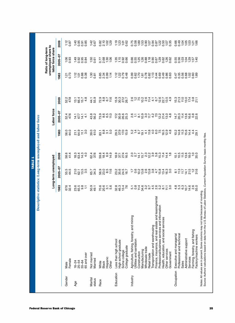
gender, age, marital status, race, education, industry, and occupational background in 2009, in 1983 (when unemployment rates last reached 10 percent—and for the sake of comparison in the aftermath of a similarly severe recession), and in 2005–07 (before the start of the recent downturn). We also compare the distributions of these characteristics to their distributions in the en-tire labor force in the second set of columns.9 In the third set of columns, we report the ratio of the share of the long-term unemployed to the share in the labor force for each group. A number above 1 would imply that long-term unemployment was unconditionally more common in that group than would be expected given their representation in the labor force.

In the early 1980s, long spells of unemployment tended to be concentrated among factory and machine workers, who made up 29 percent of the labor force but 55 percent of the long-term unemployed, or nearly twice their representation in the work force (final row of table 1). Consequently, the long-term unemployed also tended to be heavily male (first column, first row) and only one in five long spells were from individuals with at least some college education (first column, fifteenth and sixteenth rows).

In 2009, factory and machine workers (and con-struction and manufacturing workers in general), males, and those with no college education still represented a larger share of the long-term unemployed than they did of the labor force (third column versus sixth column).10 However, the long-term unemployed became sectorally more diverse.11 For example, in 2009, the long-term unemployed were more likely to come from professional and business services and finance, insurance, and real estate relative to 1983, while the share of manufactur-ing/factory workers went down. Generally, in 2009, long-term unemployment was more equally weighted across industry, occupation, education, gender, and age groups, and was therefore more representative of the labor force and the population than it had been two and a half decades ago.

Many important demographic shifts in the labor force have occurred concurrently with changes in the average length of unemployment. This has led several researchers (for example, Abraham and Shimer, 2002; Valletta, 2005; and Mukoyama and Şahin, 2009) to suggest a link between work force trends and unemploy-ment duration. These links can be caused by differences in the propensity to be rehired in a timely fashion after job loss for particular demographic groups. For example, increases in college experience, as well as the general skills that education provides, might en-able workers to be more adaptable and thus find job matches more quickly (of course, more job-specific

or industry-specific skills could potentially slow the process down).

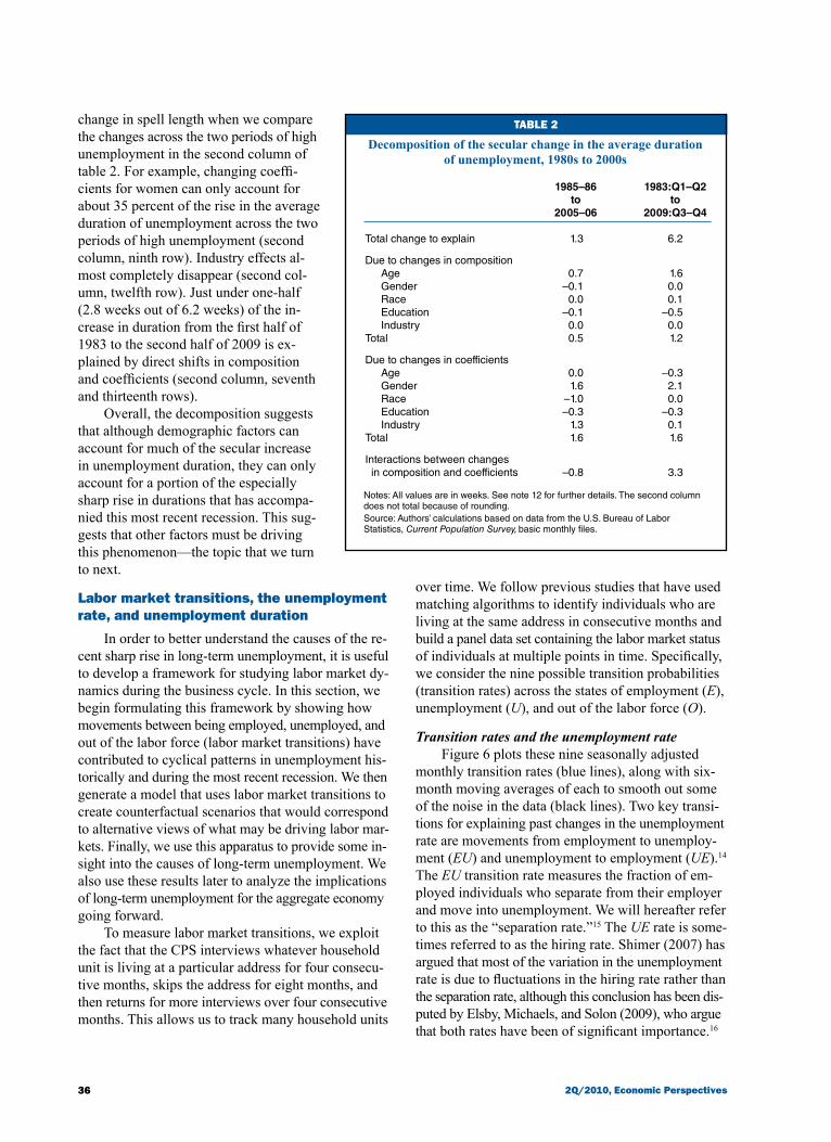
In table 2, we provide a simple breakdown of changes in average duration of unemployment, using an approach called a Blinder/Oaxaca decomposition.12 This decomposition enables us to estimate how much of the rise in unemployment duration is due to com-positional changes in the pool of unemployed workers (for example, age, gender, education, and industrial composition); how much is due to longer spell lengths within each group (for example, longer spells among women or construction workers), holding the compo-sition constant; and how much is due to interactions between changes in compositional effects and coeffi-cients. We calculate these changes over two time periods roughly 20 to 25 years apart. First, we compare 1985–86 to 2005–06, when the economy was in the midst of expansions. Second, we examine two periods in our sample where unemployment was 10 percent or higher—the first six months of 1983 and the last six months of 2009 (that is, 1983:Q1–Q2 and 2009:Q3–Q4).

We find that most changes in the composition of the work force account for little of the increase in aver-age duration of unemployment.13 The notable exception is the age structure of the population. Younger workers in the midst of a long unemployment spell tend to have shorter spells of unemployment than older workers in the same situation (Abraham and Shimer, 2002). There-fore, as the labor force has become older, average spells have tended to become longer. In table 2 (first column, second row), we show that changes in age can account for 0.7 weeks of the 1.3 increase in weeks from the mid-1980s to the mid-2000s, or about 53 percent. Yet, the changing age composition only accounts for about 25 percent of the rise in duration across the two periods of high unemployment (second column, second row). This suggests that as the baby boom generation con-tinues to transition out of the labor force over the next decade, we should expect the average duration of un-employment to slowly fall.

The results of the decomposition also suggest that rising length of unemployment among women (holding the share of women in the labor force fixed) can account for virtually the entire increase in the average duration from the mid-1980s to the mid-2000s (table 2, first col-umn, ninth row). This corresponds to the greater labor force attachment of women in recent decades and con-firms Abraham and Shimer (2002), whose findings have a similar pattern. Change in unemployment duration within industries (first column, twelfth row) can also account for some of the secular pattern across expansions.

However, both the female and industry effects can explain a notably smaller share of the total


TaB

lE 1

Des

crip

tive

stat

istic

s: L

ong-

term

une

mpl

oyed

and

labo

r fo

rce

R

atio

of

lon

g-t

erm

u

nem

plo

yed

sh

are

to

Lo

ng

-ter

m u

nem

plo

yed

L

abo

r fo

rce

lab

or

forc

e sh

are

19

83

2005

–07

2009

19

83

2005

–07

2009

19

83

2005

–07

2009

Gen

der

Mal

e 67

.6

55.5

58

.6

56.0

52

.4

52.2

1.

21

1.06

1.

12

Fem

ale

32.4

44

.5

41.4

44

.0

47.6

47

.8

0.73

0.

93

0.87

Age

16

–24

23.6

21

.0

18.3

21

.1

14.1

13

.1

1.12

1.

49

1.40

25

–54

65.5

62

.1

63.4

64

.9

67.7

66

.4

1.01

0.

92

0.95

55

–64

9.8

13.5

14

.3

11.1

14

.1

15.7

0.

88

0.95

0.

91

65 a

nd o

ver

1.1

3.5

4.0

3.0

4.1

4.8

0.38

0.

84

0.85

Mar

ital

Not

mar

ried

50.9

65

.7

62.4

39

.0

43.8

44

.1

1.30

1.

50

1.42

stat

us

Mar

ried

49.1

34

.3

37.6

61

.0

56.2

55

.9

0.81

0.

61

0.67

Rac

e W

hite

70

.6

56.9

59

.8

83.1

73

.9

72.9

0.

85

0.77

0.

82

Bla

ck

20.6

23

.0

18.4

8.

8 8.

6 8.

8 2.

34

2.68

2.

10

His

pani

c 3.

1 8.

5 6.

9 3.

1 6.

5 6.

7 0.

99

1.30

1.

02

Oth

er

5.6

11.6

14

.9

5.0

11.0

11

.6

1.14

1.

06

1.29

Edu

catio

n Le

ss th

an h

igh

scho

ol

32.8

23

.2

18.9

29

.3

17.2

15

.9

1.12

1.

35

1.19

H

igh

scho

ol g

radu

ate

46.3

35

.6

37.1

37

.9

30.9

30

.3

1.22

1.

15

1.23

S

ome

colle

ge

13.4

24

.5

27.4

17

.0

26.6

27

.2

0.79

0.

92

1.01

C

olle

ge g

radu

ate

7.6

16.7

16

.5

15.9

25

.3

26.7

0.

48

0.66

0.

62

Indu

stry

A

gric

ultu

re, f

ishi

ng, f

ores

try,

and

min

ing

5.1

1.7

2.0

5.2

2.6

2.6

0.99

0.

66

0.75

U

tiliti

es a

nd s

anita

tion

0.8

0.6

0.7

1.4

1.1

1.2

0.62

0.

55

0.58

C

onst

ruct

ion

11.4

10

.2

14.1

6.

7 8.

1 7.

5 1.

70

1.25

1.

89

Man

ufac

turin

g 34

.6

13.8

15

.7

19.1

10

.9

10.2

1.

81

1.26

1.

53

Who

lesa

le tr

ade

3.2

2.6

2.3

4.1

3.0

2.6

0.78

0.

88

0.90

R

etai

l tra

de

9.7

13.8

12

.2

11.8

11

.7

11.4

0.

82

1.18

1.

07

Tran

spor

tatio

n an

d w

areh

ousi

ng

4.5

3.8

3.9

4.0

4.2

4.1

1.13

0.

90

0.94

F

inan

ce, i

nsur

ance

, and

rea

l est

ate

and

leas

ing/

rent

al

2.6

4.7

5.8

6.0

7.0

6.7

0.44

0.

67

0.87

P

rofe

ssio

nal/b

usin

ess

serv

ices

and

info

rmat

ion

5.

2 15

.8

15.3

7.

5 12

.2

12.6

0.

69

1.29

1.

22

H

ealth

, edu

catio

n, a

nd s

ocia

l ser

vice

s 8.

1 13

.4

11.4

16

.5

21.4

22

.7

0.49

0.

62

0.50

O

ther

ser

vice

s 11

.1

16.3

14

.4

12.9

13

.0

13.5

0.

86

1.26

1.

07

Gov

ernm

ent

3.0

3.0

1.8

4.8

4.8

4.9

0.63

0.

62

0.35

Occ

upat

ion

Exe

cutiv

e an

d m

anag

eria

l 4.

8 8.

1 10

.1

10.2

14

.7

15.3

0.

47

0.55

0.

66

Pro

fess

iona

l and

tech

nica

l 5.

3 11

.3

10.5

14

.8

20.3

21

.3

0.35

0.

56

0.49

S

ales

6.

3 11

.7

11.5

11

.3

11.4

11

.0

0.56

1.

03

1.04

A

dmin

istr

ativ

e su

ppor

t 10

.7

14.1

13

.6

15.6

13

.6

13.0

0.

68

1.04

1.

05

Ser

vice

s 14

.6

21.5

18

.0

14.4

16

.6

17.4

1.

02

1.29

1.

03

Farm

ing,

fore

stry

, and

fish

ing

2.6

1.2

1.0

4.4

0.8

0.8

0.60

1.

57

1.21

Fa

ctor

y/m

achi

ne w

orke

rs

55.0

31

.6

35.0

29

.1

22.6

21

.1

1.89

1.

40

1.66

Not

es: A

ll va

lues

are

in p

erce

nt. S

ome

colu

mns

may

not

tota

l bec

ause

of r

ound

ing.

Sou

rce:

Aut

hors

’ cal

cula

tions

bas

ed o

n da

ta fr

om th

e U

.S. B

urea

u of

Lab

or S

tatis

tics,

Cur

rent

Pop

ulat

ion

Sur

vey,

bas

ic m

onth

ly fi

les.


TaBlE 2

Decomposition of the secular change in the average duration of unemployment, 1980s to 2000s

1985–86 1983:Q1–Q2 to to 2005–06 2009:Q3–Q4

Total change to explain 1.3 6.2

Due to changes in composition Age 0.7 1.6 Gender –0.1 0.0 Race 0.0 0.1 Education –0.1 –0.5 Industry 0.0 0.0Total 0.5 1.2 Due to changes in coefficients Age 0.0 –0.3 Gender 1.6 2.1 Race –1.0 0.0 Education –0.3 –0.3 Industry 1.3 0.1Total 1.6 1.6

Interactions between changes in composition and coefficients –0.8 3.3

Notes: All values are in weeks. See note 12 for further details. The second column does not total because of rounding.Source: Authors’ calculations based on data from the U.S. Bureau of Labor Statistics, Current Population Survey, basic monthly files.

change in spell length when we compare the changes across the two periods of high unemployment in the second column of table 2. For example, changing coeffi-cients for women can only account for about 35 percent of the rise in the average duration of unemployment across the two periods of high unemployment (second column, ninth row). Industry effects al-most completely disappear (second col-umn, twelfth row). Just under one-half (2.8 weeks out of 6.2 weeks) of the in-crease in duration from the first half of 1983 to the second half of 2009 is ex-plained by direct shifts in composition and coefficients (second column, seventh and thirteenth rows).

Overall, the decomposition suggests that although demographic factors can account for much of the secular increase in unemployment duration, they can only account for a portion of the especially sharp rise in durations that has accompa-nied this most recent recession. This sug-gests that other factors must be driving this phenomenon—the topic that we turn to next.

labor market transitions, the unemployment rate, and unemployment duration

In order to better understand the causes of the re-cent sharp rise in long-term unemployment, it is useful to develop a framework for studying labor market dy-namics during the business cycle. In this section, we begin formulating this framework by showing how movements between being employed, unemployed, and out of the labor force (labor market transitions) have contributed to cyclical patterns in unemployment his-torically and during the most recent recession. We then generate a model that uses labor market transitions to create counterfactual scenarios that would correspond to alternative views of what may be driving labor mar-kets. Finally, we use this apparatus to provide some in-sight into the causes of long-term unemployment. We also use these results later to analyze the implications of long-term unemployment for the aggregate economy going forward.

To measure labor market transitions, we exploit the fact that the CPS interviews whatever household unit is living at a particular address for four consecu-tive months, skips the address for eight months, and then returns for more interviews over four consecutive months. This allows us to track many household units

over time. We follow previous studies that have used matching algorithms to identify individuals who are living at the same address in consecutive months and build a panel data set containing the labor market status of individuals at multiple points in time. Specifically, we consider the nine possible transition probabilities (transition rates) across the states of employment (E), unemployment (U), and out of the labor force (O).

Transition rates and the unemployment rateFigure 6 plots these nine seasonally adjusted

monthly transition rates (blue lines), along with six-month moving averages of each to smooth out some of the noise in the data (black lines). Two key transi-tions for explaining past changes in the unemployment rate are movements from employment to unemploy-ment (EU) and unemployment to employment (UE).14 The EU transition rate measures the fraction of em-ployed individuals who separate from their employer and move into unemployment. We will hereafter refer to this as the “separation rate.”15 The UE rate is some-times referred to as the hiring rate. Shimer (2007) has argued that most of the variation in the unemployment rate is due to fluctuations in the hiring rate rather than the separation rate, although this conclusion has been dis-puted by Elsby, Michaels, and Solon (2009), who argue that both rates have been of significant importance.16


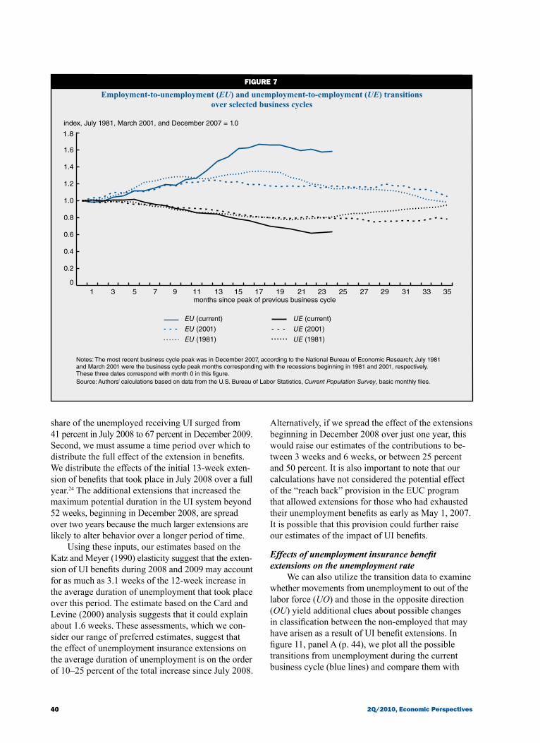
Movements in the EU have been particularly pro-nounced in this recession: The separation rate has risen by nearly 70 percent. This disproportionate hike is shown more clearly in figure 7 (p. 40), where we compare the proportional change in the EU and UE transition rates in the current business cycle with the recessionary periods in 1981–82 and 2001. The EU transition rate followed its historical pattern during 2008 but then began rising sharply early in 2009. Relative to the acceleration in the EU rate, the UE rate appears to have fallen more gradually, though proportionately more than in previous recessions.

To assess how important the transitions out of employment versus transitions out of unemployment have been in explaining the rise in the unemployment rate during the most recent downturn, we perform some simple simulations. We start with the actual levels of those who are employed, unemployed, and out of the labor force and the smoothed values of all nine of the labor market transition rates at the end of 2007. We then use the actual transition rates starting in January 2008 to simulate the new counts of individuals in each labor market state for each month going forward. This is described in greater detail in box 1 (p. 41). With some basic adjustments, we are able to match the actual monthly unemployment rates through the end of 2009 almost perfectly.

We then conduct the following two experiments. First, we hold all transition rates constant at their December 2007 values except for the three transitions that start with the employment state in the initial month (EE, EU, and EO).17 Those transition rates are allowed to vary according to what actually transpired in 2008 and 2009. In essence, this exercise, which is plotted as the dark blue line on figure 8 (p. 42), captures the effects of transitions out of employment into non- employment (being either unemployed or out of the labor force) on the aggregate unemployment rate.18 Analogously, we do a second experiment where only the transitions from the state of unemployment (UE, UU, and UO) are allowed to change. This captures the effects of the fall in the exit rate out of unemploy-ment into being either employed or out of the labor force. Those results are shown as the light blue line in figure 8. The black line is the actual unemployment rate, and the gray one is the actual unemployment rate in December 2007.

We find that the changes in the transition rates out of employment (all else being equal) would only raise the unemployment rate by 1 percentage point by the end of 2009. In contrast, changes in the transition rates out of unemployment would raise the unemploy-ment rate by 2.2 percentage points. Broadly speaking,

this suggests that the combined effects of moving out of unemployment (UE, UU, and UO)—including, prominently, the transition into a job—explain more of the actual increase in the unemployment rate over the past two years than the combined effects of mov-ing out of employment (EE, EU, and EO).19

Transition rates and unemployment durationWe next turn to using these exercises to explain

unemployment duration. The simulation is similar as before except that we now explicitly incorporate the distribution of unemployment duration into the analysis by using five-week “bins” of unemployment spells (that is, 0–4 weeks, 5–9 weeks, and so on). We start with the distribution of unemployment duration at the end of 2007 and use estimates of the actual transition rates into and out of unemployment for each bin, along with estimates for the other transition rates, to update the distribution of duration each month. We again find that the simulation does extremely well at replicating the sharp rise in the average duration of unemployment during 2009.20

In figure 9 (p. 42), we show that if only the EE, EU, and EO followed their actual paths and all the other transition rates stayed constant at their December 2007 values, the average duration of unemployment would have only increased slightly, to about 19 weeks by the end of 2009 (dark blue line). If, however, only UE, UU, and UO followed their actual paths and the other tran-sition rates stayed flat, unemployment duration would have increased to nearly 23 weeks (light blue line). So it appears that for both the unemployment rate and the average duration of unemployment, transition rates from the starting state of unemployment have been the im-portant driving influences.21

Simulated effects of federal unemployment insurance benefit extensions

As noted previously, the spike in the average dura-tion of unemployment starting in mid-2009 is hard to explain using demographics or the standard association with deteriorating GDP growth. One plausible explana-tion is the unprecedented extension of unemployment insurance benefits. The maximum number of weeks of eligibility rose from 26 weeks to 39 weeks in July 2008 with the passage and creation of the Emergency Unemployment Compensation (EUC) federal program. Since then, extensions have risen at varying rates, de-pending on the unemployment situation of individual states.22 Figure 10 (p. 43) plots the weighted national average of the maximum number of weeks of unem-ployment benefit receipt allowed (blue line); the weights for this average are based on the size of the unemployment pool in each state. As of January 2010,


A. E

mp

loym

ent

to e

mp

loym

ent

tran

sitio

n ra

te

Lab

or m

arke

t tra

nsiti

on r

ates

, 197

6–20

09FI

gu

RE 6

B. U

nem

plo

ymen

t to

em

plo

ymen

ttr

ansi

tion

rate

C. O

ut

of

the

lab

or

forc

e to

em

plo

ymen

ttr

ansi

tion

rate

D. E

mp

loym

ent

to u

nem

plo

ymen

ttr

ansi

tion

rate

E. U

nem

plo

ymen

t to

un

emp

loym

ent

tran

sitio

n ra

teF.

Ou

t o

f th

e la

bo

r fo

rce

to u

nem

plo

ymen

ttr

ansi

tion

rate

1976

’80

’84

’88

’92

’96

2000

’04

’08

1976

’80

’84

’88

’92

’96

2000

’04

’08

0.10

0.15

0.20

0.25

0.30

0.35

0.40

1976

’80

’84

’88

’92

’96

2000

’04

’08

0.02

0.03

0.04

0.05

0.06

0.07

1976

’80

’84

’88

’92

’96

2000

’04

’08

0.00

0

0.00

5

0.01

0

0.01

5

0.02

0

0.02

5

0.03

0

1976

’80

’84

’88

’92

’96

2000

’04

’08

1976

’80

’84

’88

’92

’96

2000

’04

’08

0.01

0.02

0.03

0.04

0.05

0.06

0.94

0

0.94

5

0.95

0

0.95

5

0.96

0

0.96

5

0.97

0

0.40

0.45

0.50

0.55

0.60

0.65

0.70


unemployed workers in 14 states were allowed the maximum of 99 weeks of UI benefits and the na-tional average was 90 weeks. By contrast, in 1983, the maximum potential duration of UI coverage in any state had reached 55 weeks.

In order to estimate the possible effect of UI benefit extensions on unemployment duration, we use previous studies of the effect of an additional week of maximum benefits on average duration. A prominent example in this literature is Katz and Meyer (1990), who use a rich statistical model and administrative data from the UI system to estimate the probability of leaving unemployment during the early 1980s recessions. They identify the impact of UI through variation in maximum benefits both within and across states that shift as a result of eli-gibility rules and legislative changes. They find that the average duration of unemployment rises by 0.16 weeks to 0.2 weeks for each additional week of benefits extended.

Katz and Meyer (1990) face the difficult prob-lem of disentangling the effects of UI benefit exten-sions from the effects of poor economic conditions that typically prompt benefit extensions in the first place. When the economy is in a recession, longer spells of unemployment are expected irrespective of the generosity of the unemployment insurance program. To get around this problem, Card and Levine (2000) use an increase in the maximum number of weeks of benefit eligibility in New Jersey in 1996; this increase was unrelated to the state of the economy at the time. In fact, this particular ex-tension, which was driven by political considerations, took place in the midst of an expansion and there-fore might be less susceptible to the bias of reces-sion-driven extensions. Indeed, they find a smaller effect than Katz and Meyer (1990) and much of the rest of the literature; mean duration rises by about 0.1 weeks for each additional week of bene-fits. In order to reflect our uncertainty over the true effect, we use both estimates.

We begin our analysis in June 2008, when maxi-mum UI eligibility was 26 weeks and unemploy-ment spells lasted about 17 weeks on average (the six-month mean from January through June 2008). We then calculate an estimated effect of the exten-sion in unemployment benefits for each subsequent month beginning with July 2008.23 For such a calcu-lation, two additional inputs are required. First, we need the share of the unemployed who are actually receiving benefits because they are the only ones who would be directly affected by policy changes. The black line in figure 10 (p. 43) shows that the

G. E

mp

loym

ent

to o

ut

of

the

lab

or

forc

etr

ansi

tion

rate

Lab

or m

arke

t tra

nsiti

on r

ates

, 197

6–20

09FI

gu

RE 6

(c

ontinued)

H. U

nem

plo

ymen

t to

ou

t o

f th

e la

bo

r fo

rce

tran

sitio

n ra

teI.

Ou

t o

f th

e la

bo

r fo

rce

to o

ut

of

the

lab

or

forc

etr

ansi

tion

rate

Not

es: A

ll tr

ansi

tion

rate

s ar

e se

ason

ally

adj

uste

d an

d pl

otte

d as

blu

e lin

es, a

nd th

eir

six-

mon

th m

ovin

g av

erag

es a

re p

lotte

d as

bla

ck li

nes.

Tra

nsiti

on r

ates

are

not

ava

ilabl

e fo

r so

me

mon

ths,

whe

n m

atch

ing

indi

vidu

als

was

not

pos

sibl

e be

caus

e of

sur

vey

rede

sign

s.S

ourc

e: A

utho

rs’ c

alcu

latio

ns b

ased

on

data

from

the

U.S

. Bur

eau

of L

abor

Sta

tistic

s, C

urre

nt P

opul

atio

n S

urve

y, b

asic

mon

thly

file

s.

1976

’80

’84

’88

’92

’96

2000

’04

’08

1976

’80

’84

’88

’92

’96

2000

’04

’08

0.10

0.15

0.20

0.25

0.30

0.35

0.40

0.02

0

0.02

5

0.03

0

0.03

5

0.04

0

0.04

5

0.05

0

0.90

0.91

0.92

0.93

0.94

0.95 19

76’8

0’8

4’8

8’9

2’9

620

00’0

4’0

8


index, July 1981, March 2001, and December 2007 = 1.0

Employment-to-unemployment (EU) and unemployment-to-employment (UE) transitions over selected business cycles

FIguRE 7

Notes: The most recent business cycle peak was in December 2007, according to the National Bureau of Economic Research; July 1981 and March 2001 were the business cycle peak months corresponding with the recessions beginning in 1981 and 2001, respectively. These three dates correspond with month 0 in this figure.Source: Authors’ calculations based on data from the U.S. Bureau of Labor Statistics, Current Population Survey, basic monthly files.

share of the unemployed receiving UI surged from 41 percent in July 2008 to 67 percent in December 2009. Second, we must assume a time period over which to distribute the full effect of the extension in benefits. We distribute the effects of the initial 13-week exten-sion of benefits that took place in July 2008 over a full year.24 The additional extensions that increased the maximum potential duration in the UI system beyond 52 weeks, beginning in December 2008, are spread over two years because the much larger extensions are likely to alter behavior over a longer period of time.

Using these inputs, our estimates based on the Katz and Meyer (1990) elasticity suggest that the exten-sion of UI benefits during 2008 and 2009 may account for as much as 3.1 weeks of the 12-week increase in the average duration of unemployment that took place over this period. The estimate based on the Card and Levine (2000) analysis suggests that it could explain about 1.6 weeks. These assessments, which we con-sider our range of preferred estimates, suggest that the effect of unemployment insurance extensions on the average duration of unemployment is on the order of 10–25 percent of the total increase since July 2008.

Alternatively, if we spread the effect of the extensions beginning in December 2008 over just one year, this would raise our estimates of the contributions to be-tween 3 weeks and 6 weeks, or between 25 percent and 50 percent. It is also important to note that our calculations have not considered the potential effect of the “reach back” provision in the EUC program that allowed extensions for those who had exhausted their unemployment benefits as early as May 1, 2007. It is possible that this provision could further raise our estimates of the impact of UI benefits.

Effects of unemployment insurance benefit extensions on the unemployment rate

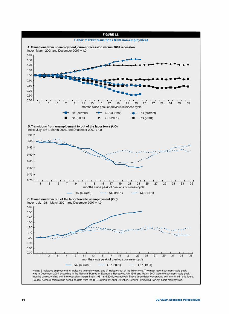
We can also utilize the transition data to examine whether movements from unemployment to out of the labor force (UO) and those in the opposite direction (OU) yield additional clues about possible changes in classification between the non-employed that may have arisen as a result of UI benefit extensions. In figure 11, panel A (p. 44), we plot all the possible transitions from unemployment during the current business cycle (blue lines) and compare them with

1 3 5 7 9 11 13 15 17 19 21 23 25 27 29 31 33 350

0.2

0.4

0.6

0.8

1.0

1.2

1.4

1.6

1.8

EU (current)

EU (2001)

EU (1981)

UE (current)

UE (2001)

UE (1981)

months since peak of previous business cycle


BOX 1

Methodology for simulating paths of the unemployment rate and unemployment durations

In this article, we use transitions across different labor market states as a tool for simulating the paths of the unemployment rate and unemployment dura-tions. This allows us to consider alternative scenarios for the path of the unemployment rate or durations either historically or going forward based on changing the paths of particular transitions. Using this approach, we can infer the relative importance of particular economic phenomena that are related to certain tran-sitions as described in the text. An important caveat is that this is a mechanical approach that may or may not correspond well to changes in the actual economy. For example, conditions that may change a particular transition rate may also affect other transition rates in ways that we may not consider.

If we consider time as discrete and denote it as t and let x stand for a particular labor market state, that is, employed, unemployed, or out of the labor force, (x = {E,U,O}), then each of the nine possible transitions are defined as the probability of being in a particular labor market state in t conditional on having been in the same or different labor market state in the prior period. For example, the EU transition is defined as:

EU = Prob (xt = U|xt–1 = E).

For each initial state in t – 1, the three possible transitions must sum to 1. For example, EE + EU + EO = 1. Each of the nine transitions for each month is estimated empirically using the matched Current Population Survey as described in the text. To imple-ment the simulation we start by inputting the levels of those who are employed, unemployed, and out of the labor force for a chosen base period. We then simulate the next period’s level of E, U, and O, using the assumed levels for the base period and an assumed path for the transition probabilities. For example, if we wish to simulate the actual path of the unemployment rate through 2008 and 2009, we define December 2007 as our base period and then use the actual estimated values of the transition probabilities for January 2008 through December 2009.1

For example:

EJan08 = EDec07 × EEJan08 + UDec07 × EUJan08 + ODec07 × EOJan08.

We use several methods to pose alternative tran-sition rates, depending on our question of interest. To address the relative importance of transitions from employment versus transitions from unemployment, we start with a baseline path where all of the transi-tion rates are constant. We then change the paths of all three transition rates from either employment or unemployment simultaneously. For example, we sim-ulate the effects arising only from changes from the employment state by changing the paths of EE, EU, and EO simultaneously.

A second approach is used when we wish to hold the UO and OU transition rates fixed at a particular rate. In this case, we allow the UE and OE rates to fol-low their actual paths and then adjust the UU and OO so that the probabilities from U and from O each sum to 1. Finally, for the simulation that attempts to repro-duce the forecast of the unemployment rate according to the Blue Chip Economic Indicators, we assume that the EU, EE, UU, and UE rates take five years to return to their historical average values. We then ad-just the EO and UO rates so that the three transitions from E and from U sum to 1.

1Rather than immediately going from the base period to the first period of the simulation, we first use the transition rates from the base period and run about ten iterations of the model so that the values of E, U, and O and the implied unemploy-ment rate reach a steady state, where they are unchanging. We then proceed to use the steady-state values for the simulation. The steady-state values may differ from the actual values in the base period. For example, the steady-state value of the unemploy-ment rate in December 2007 is about 80 percent of the actual value. We therefore scale the subsequent values of the simula-tion by a factor of 1.25. This discrepancy is likely due in part to the inability to account for month-to-month compositional changes that arise from the fact that individuals enter or exit the working age population. Measurement error and differences between the complete population and the matched sample may also play a role. This approach assumes that although we can-not match the level of unemployment, we can match changes over time.

those during the 2001 recession and its aftermath (black lines). The series with the boxes represent the UE transition rates and are identical to those shown in figure 7 (p. 40). To this we add UU transition rates (diamonds) and UO (circles) rates. It appears that the UU and UO rates in the current recession track the rates in 2001 reasonably well for the first 16 or so months of the downturn before beginning to diverge. In con-trast, the UE rates diverge earlier in the cycle. One

possible reason for this pattern is that individuals who would have normally dropped out of the labor force at this point in the cycle chose to remain unemployed—perhaps to continue to collect unemployment benefits.

In figure 11, panel B (p. 44), we focus only on the rate of UO transitions and add data from the 1981–82 recession (dotted). This panel shows that the UO path during the current recession resembles the UO path dur-ing the 1981–82 recession reasonably well, suggesting


percent

Counterfactual effects of changing labor market transition rates on the unemployment rate, 2008–09FIguRE 8

Note: E indicates employment, U indicates unemployment, and O indicates out of the labor force.Sources: Authors’ calculations based on data from the U.S. Bureau of Labor Statistics, Current Population Survey, basic monthly files; and Haver Analytics.

weeks

Counterfactual effects of changing labor market transition rates on the duration of unemployment, 2008–09FIguRE 9

Notes: E indicates employment, U indicates unemployment, and O indicates out of the labor force. The average duration of unemployment in December 2007 was about 17 weeks, so we use this duration as our baseline.Source: Authors’ calculations based on data from the U.S. Bureau of Labor Statistics, Current Population Survey, basic monthly files.

Jan Mar May Jul Sep Nov Jan Mar May Jul Sep Nov0

2

4

6

8

10

12

Actual unemployment rate

Unemployment rate if only EE, EU, and EO change

2008 2009

Unemployment rate if only UE, UU, and UO change

Unemployment rate in December 2007

0

5

10

15

20

25

30

35

Jan Mar May Jul Sep Nov Jan Mar May Jul Sep Nov

Actual average duration of unemployment

Average duration of unemployment if only EE, EU, and EO change

2008 2009

Average duration of unemployment if only UE, UU, and UO change

Baseline duration, 17 weeks


weeks

Maximum potential duration of unemployment insurance (UI) benefits and the share of unemployed receiving benefits, 2008–09

FIguRE 10

Notes: The weights for the national average duration are based on the size of the unemployment pool in each state. The share of unemployed receiving UI benefits is the number of individuals with continuing claims under federal and state unemployment insurance programs divided by the number of unemployed; this fraction is seasonally adjusted. Sources: Authors’ calculations based on data from the U.S. Department of Labor, the U.S. Bureau of Labor Statistics, and Haver Analytics.

share receiving benefits

that the departure from the 2001 pattern may simply reflect the greater severity of the current recession. That said, figure 11, panel C suggests that the rate of OU transitions in the current recession appears to move substantially higher in percentage terms than the patterns observed during the previous downturns.

We conduct a simulation motivated by figure 11 to ask how different the unemployment rate would be had the paths of the UO and OU transitions stayed con-stant at their values 16 months after the start of the recession (April 2009). In order to ensure that the proba-bilities from a particular state add up to 1, we allow the UE and OE rates to follow their actual paths and adjust the UU and OO rates so that the probabilities sum to 1. Figure 12 shows that under this counterfac-tual scenario the result of this exercise would be to lower the unemployment rate to 9.3 percent as of December 2009—about 0.7 percentage points below the actual unemployment rate that month. Although this is a relatively crude and mechanical approach, it nonetheless provides a magnitude for the possible effect of unemployment insurance benefit extensions on the unemployment rate.

Implications of long-term unemployment for the aggregate economy

In this section, we consider how the increase in long-term unemployment may affect the economy going forward. We consider the effects of the unemployment duration structure on the unemployment rate and then on compensation growth.

Effects of duration structure on the unemployment rate

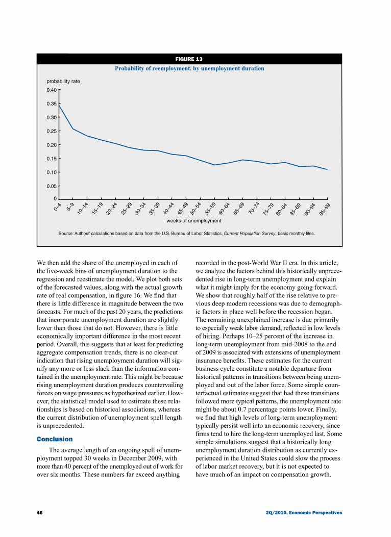
As unemployment spells lengthen, the probability of finding a job in a given time period declines—an association that is robust across time and demographic groups. The pattern is illustrated in figure 13 (p. 46), which plots the probability of being employed today for various lengths of unemployment duration in the previous month (horizontal axis). For example, at 0–4 weeks of unemployment, the average probability of finding a job in the following month is 34 percent, but at 25–29 weeks, it is only 19 percent.25 As much as this phenomenon is due to diminished job skills and weakened social networks, it could have a real impact on the labor market recovery while the broader economic recovery takes hold.

0

10

20

30

40

50

60

70

80

90

0

0.1

0.2

0.3

0.4

0.5

0.6

0.7


Maximum potential duration of UI benefits, weighted national average (left-hand scale)

Share of unemployed receiving UI benefits (right-hand scale)

2008 2009


A. Transitions from unemployment, current recession versus 2001 recessionindex, March 2001 and December 2007 = 1.0

Labor market transitions from non-employmentFIguRE 11

Notes: E indicates employment, U indicates unemployment, and O indicates out of the labor force. The most recent business cycle peak was in December 2007, according to the National Bureau of Economic Research; July 1981 and March 2001 were the business cycle peak months corresponding with the recessions beginning in 1981 and 2001, respectively. These three dates correspond with month 0 in this figure.Source: Authors’ calculations based on data from the U.S. Bureau of Labor Statistics, Current Population Survey, basic monthly files.

B. Transitions from unemployment to out of the labor force (UO)index, July 1981, March 2001, and December 2007 = 1.0

C. Transitions from out of the labor force to unemployment (OU)index, July 1981, March 2001, and December 2007 = 1.0

OU (current) OU (2001) OU (1981)

1.60

1.40

1.30

1.20

1.10

1.00

0.90

0.80

0.70

1.50

1 3 5 7 9 11 13 15 17 19 21 23 25 27 29 31 33 35months since peak of previous business cycle

UE (current) UU (current) UO (current)

UE (2001) UU (2001) UO (2001)

1.40

1.20

1.10

1.00

0.90

0.80

0.70

0.60

0.50

1.30


UO (current) UO (2001) UO (1981)

1.05

0.95

0.90

0.85

0.80

0.75

0.70

1.00



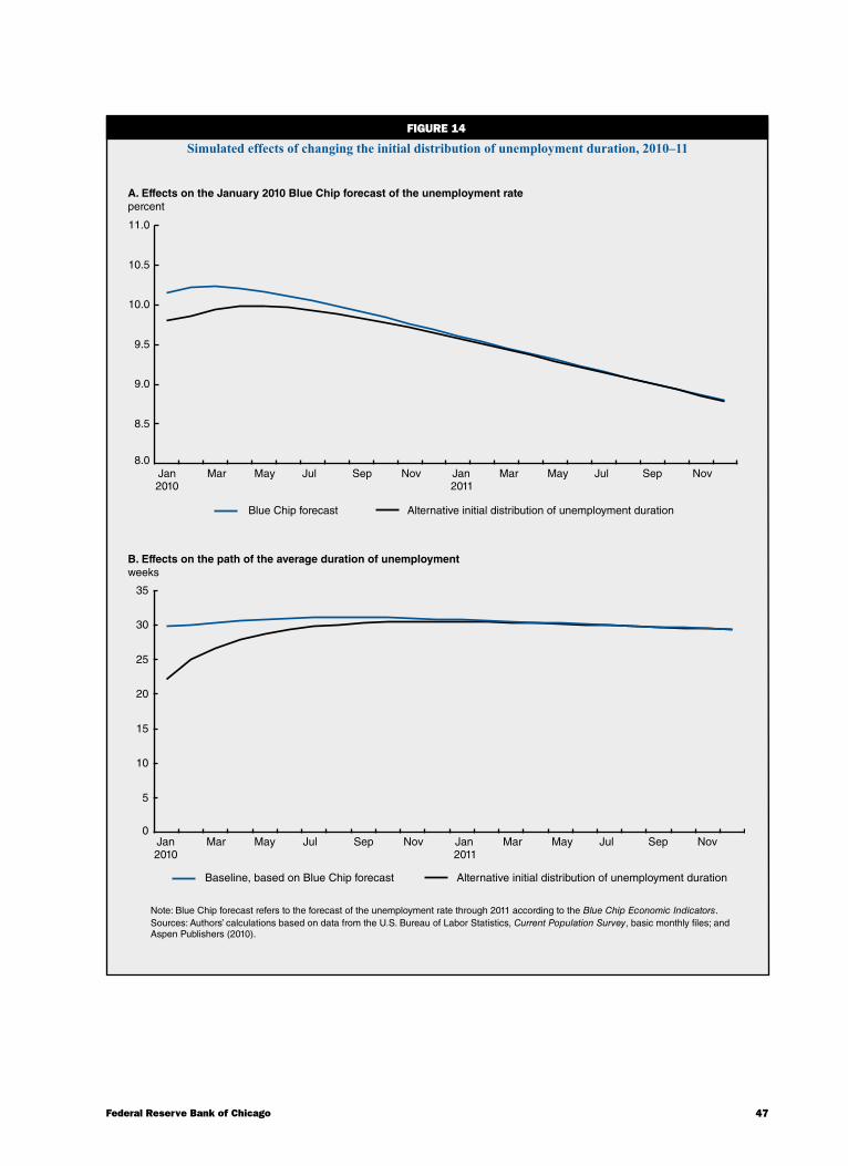
In order to investigate this possibility, we use our transition rate model but substitute aggregate transition rate probabilities for movement from unemployment (UE, UU, and UO) with analogous transition rate proba-bilities for each five-week bin of unemployment dura-tion. We start by simulating a baseline path that roughly matches the January 10, 2010, forecast of the unemploy-ment rate through 2011 according to the Blue Chip Economic Indicators (Blue Chip), a survey of America’s top business economists (Aspen Publishers, 2010). We then pose an alternative path where the only change is to make the share of the unemployed in each five-week bin at the beginning of the simulation (January 2010) match their mean historical values. In figure 14, panel A, we show that this alternative initial distribution of duration would immediately lower the unemployment rate by about 0.4 percentage points relative to the Blue Chip path. We find, however, that duration quickly re-verts back to high levels (figure 14, panel B) and that the unemployment rate path converges to what it would have been had the model started with the actual dis-tribution of duration. The main lesson we take from this exercise is that the unemployment rate is probably about half a point higher than it would be if unemploy-ment spell lengths were at more historical levels.

Effects of duration structure on compensation growthLastly, we consider the possible effects of higher

long-term unemployment rates on aggregate wage growth. It is not obvious a priori what the expected effects should be. If the long-term unemployed are readily employable and can fulfill vacancies, then there is a sense in which they may be more eager to return to work at the prevailing wage than individuals with short unemployment durations. In this case, the long-term unemployed may reduce wage pressures. If, how-ever, many of the long-term unemployed are more akin to individuals who have stopped searching for work and have left the labor force, perhaps because of a geographical or skills mismatch, then they may play little role in bidding down wages.

Since this is ultimately an empirical question, we undertake a simple exercise using Phillips curve style regressions to address this. We use data on year-over-year growth in real compensation per hour. Figure 15 (p. 48) shows that, as expected, there is a negative rela-tionship between compensation growth and the unem-ployment rate. The black boxes signify the values starting with 2008:Q1, when the recession began. We regress compensation growth on the unemployment rate for the post-1975 period and calculate the predicted values.

percent

Counterfactual effects of holding unemployment-to-out-of-the-labor-force (UO)and out-of-the-labor-force-to-unemployment (OU) transition rates fixed from April 2009 onward

on the unemployment rate, 2008–09

FIguRE 12

Sources: Authors’ calculations based on data from the U.S. Bureau of Labor Statistics, Current Population Survey, basic monthly files; and Haver Analytics.

4

5

6

7

8

9

10

11

Jan Mar May Jul Sep Nov Jan Mar May Jul Sep Nov2008 2009

Actual unemployment rate

Simulated unemployment rate, with UO and OU fixed


probability rate

Probability of reemployment, by unemployment durationFIguRE 13

Source: Authors’ calculations based on data from the U.S. Bureau of Labor Statistics, Current Population Survey, basic monthly files.

0–4

10–1

4

15–1

920

–24

25–2

930

–34

35–3

940

–44

45–4

950

–54

55–5

960

–64

65–6

9

70–7

475

–79

80–8

485

–89

90–9

4

95–9

9

0

0.05

0.10

0.15

0.20

0.25

0.30

0.35

0.40

5–9

weeks of unemployment

We then add the share of the unemployed in each of the five-week bins of unemployment duration to the regression and reestimate the model. We plot both sets of the forecasted values, along with the actual growth rate of real compensation, in figure 16. We find that there is little difference in magnitude between the two forecasts. For much of the past 20 years, the predictions that incorporate unemployment duration are slightly lower than those that do not. However, there is little economically important difference in the most recent period. Overall, this suggests that at least for predicting aggregate compensation trends, there is no clear-cut indication that rising unemployment duration will sig-nify any more or less slack than the information con-tained in the unemployment rate. This might be because rising unemployment duration produces countervailing forces on wage pressures as hypothesized earlier. How-ever, the statistical model used to estimate these rela-tionships is based on historical associations, whereas the current distribution of unemployment spell length is unprecedented.

Conclusion

The average length of an ongoing spell of unem-ployment topped 30 weeks in December 2009, with more than 40 percent of the unemployed out of work for over six months. These numbers far exceed anything

recorded in the post-World War II era. In this article, we analyze the factors behind this historically unprece-dented rise in long-term unemployment and explain what it might imply for the economy going forward. We show that roughly half of the rise relative to pre-vious deep modern recessions was due to demograph-ic factors in place well before the recession began. The remaining unexplained increase is due primarily to especially weak labor demand, reflected in low levels of hiring. Perhaps 10–25 percent of the increase in long-term unemployment from mid-2008 to the end of 2009 is associated with extensions of unemployment insurance benefits. These estimates for the current business cycle constitute a notable departure from historical patterns in transitions between being unem-ployed and out of the labor force. Some simple coun-terfactual estimates suggest that had these transitions followed more typical patterns, the unemployment rate might be about 0.7 percentage points lower. Finally, we find that high levels of long-term unemployment typically persist well into an economic recovery, since firms tend to hire the long-term unemployed last. Some simple simulations suggest that a historically long unemployment duration distribution as currently ex-perienced in the United States could slow the process of labor market recovery, but it is not expected to have much of an impact on compensation growth.


A. Effects on the January 2010 Blue Chip forecast of the unemployment ratepercent

Simulated effects of changing the initial distribution of unemployment duration, 2010–11FIguRE 14

Note: Blue Chip forecast refers to the forecast of the unemployment rate through 2011 according to the Blue Chip Economic Indicators.Sources: Authors’ calculations based on data from the U.S. Bureau of Labor Statistics, Current Population Survey, basic monthly files; and Aspen Publishers (2010).

B. Effects on the path of the average duration of unemploymentweeks

8.0

8.5

9.0

9.5

10.0

10.5

11.0


Blue Chip forecast Alternative initial distribution of unemployment duration

2010 2011

0

5

10

15

20

25

30

35


Baseline, based on Blue Chip forecast Alternative initial distribution of unemployment duration

2010 2011


real compensation, percent change from a year ago

Real compensation growth versus the unemployment rate, 1949–2009FIguRE 15

Note: The black line represents the relationship between the unemployment rate and the percent change of compensation from a year ago over the period 1949–2009.Source: Authors’ calculations based on data from the U.S. Bureau of Labor Statistics from Haver Analytics.

percent change from a year ago

Real compensation growth, actual versus predicted, 1949–2009FIguRE 16

Source: Authors’ calculations based on data from the U.S. Bureau of Labor Statistics from Haver Analytics.

1949 ’54 ’59 ’64 ’69 ’74 ’79 ’84 ’89 ’94 ’99 2004 ’09–8

–6

–4

–2

0

2

4

6

8

10

12

Actual

Predicted based on the unemployment rate only

Predicted based on the unemployment rate and unemployment duration

–10

–5

0

5

10

15

0 2 4 6 8 10 12unemployment rate

1949:Q1–2007:Q4 2008:Q1–2009:Q4


NOTES

1Alternatively, the relationship between the length of time out of work and the diminishment of work prospects could be picking up unobserved differences in worker quality between those who are unemployed for short and long spells (Ham and Rea, 1987; Kiefer, 1988; and Machin and Manning, 1999). In this case, longer spells in and of themselves do not lead to worse outcomes. It is very diffi-cult to convincingly identify which of these channels dominates without strong statistical assumptions.

2Based on transition patterns between being employed, unemployed, and out of the labor force altogether, we estimate that UI extensions increased the unemployment rate by roughly 0.7 percentage points during 2008–09.

3Long-term unemployment is a good deal less common in the United States than in much of the developed world (for example, Machin and Manning, 1999). As of 2008, the last year for which comparable data are available, the share of the unemployed out of work more than six months was two times, and in some cases four times, higher in Belgium, the Czech Republic, France, Germany, Greece, Hungary, Italy, Luxembourg, the Netherlands, Portugal, Switzerland, the United Kingdom, and Japan.

4The most recent numbers from the Current Population Survey are still well below the prevalence of long-term unemployment during the Great Depression. Unfortunately, national data on un-employment duration before World War II are not systematically available. Definitions of unemployment also varied across surveys and are different from the modern one. That said, Eichengreen and Hatton (1988) report that more than a third of males who were looking for work in 1930 had been unemployed for at least 14 weeks and 55 percent of ongoing unemployment spells had lasted at least six months in 1940. Eichengreen and Hatton also reproduce data from Woytinsky (1942), showing the year-to-year changes in un-employment duration in Philadelphia during the 1930s. In 1933, for example, over 80 percent of the unemployed had spells of at least six months. Chatterjee and Corbae (2007) describe a special January 1931 census of the unemployed in Boston, New York, Philadelphia, Chicago, and Los Angeles, which reported that 45 percent, 61 percent, 45 percent, 61 percent, and 33 percent were jobless for at least 18 weeks, respectively.

5As can also be seen in figures 1 and 2 (p. 30), it took particularly long for average and median unemployment duration and the share of the long-term unemployed to return to pre-recession levels fol-lowing the 1990–91 and 2001 recessions.

6The U-6 rate, available since 1994, includes marginally attached workers and part-time workers who want and are available for full-time work but had to settle for a part-time schedule for economic reasons. The U.S. Bureau of Labor Statistics classifies individuals as “marginally attached” if they “indicate that they want and are available for a job and have looked for work sometime in the re-cent past” but are not currently looking. We derived a simulated U-6 series from 1978 onward based on similar questions in the CPS. The simulated series replicates the actual reported series from 1994 onward.

7Okun’s law simply states a linear negative relationship exists between economic activity (that is, GDP growth) and the unem-ployment rate.

8To be clear, there are other series that are hard to forecast within this simple statistical model. We also underpredict the increase in those who are part-time workers for economic reasons and the frac-tion of the population outside of the labor force but not marginally attached. These results are not reported but available upon request.

9All of the inferences here are the same if the base of comparison is the full population rather than the labor force.

10This is true even when controlling simultaneously for all of the characteristics listed in table 1 (p. 35) in a regression framework

11See Aaronson and Sullivan (1998) for similar results on job displacement and job insecurity.

12To implement the Blinder/Oaxaca decomposition, a separate re-gression is run for each time period. The change in average duration of unemployment over the two periods is then decomposed into a portion due to changes in the levels of the explanatory variables (for example, the fraction of females and the fraction that has completed less than high school), a portion due to changes in the coefficients on these explanatory variables, and a residual term that captures the effects of the interactions (that is, simultaneously changing the levels and coefficients).

Specifically, let unemployment duration Dit be specific to an individual i and a time period t. To keep things simple, we use two time periods—the 1980s, which is indexed as t = 1, and the 2000s, which is indexed as t = 2. We show the results by comparing ex-pansions (1985–86 versus 2005–06 in the first column of table 2 on p. 36) and comparing periods of high unemployment (first half of 1983 versus second half of 2009 in table 2, second column). Duration is determined by characteristics Xit (for example, gender and age) that are also specific to individual i and time period t.

We can write this statistical model as Dit = Xitbt + eit , where eit is an error term. The decomposition is then D1 – D2 = (X1 – X2)b2 + X2(b1 – b2) + (X1 – X2)(b1 – b2). The first term after the equal sign is reported in the first set of rows in table 2 (“due to changes in com-position”). The second term is reported in the second set of rows (“due to changes in coefficients”), and the third term is the row labeled “interactions between changes in composition and coefficients.”

Running this decomposition on the share of the unemployed undergoing long-term spells of unemployment yields similar results. Those are available upon request.

13Notably, changes in industrial structure have little impact. See, for example, Rissman (2009), Valletta and Cleary (2008), and Aaronson, Rissman, and Sullivan (2004) on the role of sectoral reallocation on labor market conditions during recent recessions.

14Movements between being in and out of the labor force play a much smaller role in explaining shifts in the unemployment rate, so this discussion largely abstracts from these transitions for simplicity. But we return to transitions between being unemployed and out of the labor force (UO and OU) during the most recent recession later in the article.

15The term “separations,” however, is often used elsewhere to represent all transitions out of a particular job, including job-to-job transitions. The separation and hiring rates reported in the U.S. Bureau of Labor Statistics’ Job Openings and Labor Turnover Survey (JOLTS) and Business Employment Dynamics (BED) survey also include out of the labor force transitions.

16Mazumder (2008), using the U.S. Census Bureau’s Survey of Income and Program Participation (SIPP), also finds that the separation rate has been of somewhat greater importance in recent recessions than suggested by Shimer (2007).

17Typically, EE is a continuously employed person. However, it can also be someone who transitions from one job to another without a spell of non-employment.


REFERENCES

Aaronson, Daniel, Scott Brave, and Shani Schechter, 2009, “How does labor adjustment in this recession compare with the past?,” Chicago Fed Letter, Federal Reserve Bank of Chicago, No. 263, June.

Aaronson, Daniel, and Daniel G. Sullivan, 1998, “The decline of job security in the 1990s: Displace-ment, anxiety, and their effect on wage growth,” Economic Perspectives, Federal Reserve Bank of Chicago, Vol. 22, No. 1, First Quarter, pp. 17–43.

Aaronson, Daniel, Ellen R. Rissman, and Daniel G. Sullivan, 2004, “Can sectoral reallocation explain the jobless recovery?,” Economic Perspectives, Federal Reserve Bank of Chicago, Vol. 28, No. 2, Second Quarter, pp. 36–49.

Abraham, Katherine G., and Robert Shimer, 2002, “Changes in unemployment duration and labor force attachment,” in The Roaring Nineties: Can Full Employment Be Sustained?, Alan B. Krueger and Robert M. Solow (eds.), New York: Russell Sage Foundation and Century Foundation, pp. 367–420.

Aspen Publishers, 2010, “Quarterly Blue Chip forecasts,” Blue Chip Economic Indicators, Vol. 35, No. 1, January 10, p. 5.

Blanchard, Olivier Jean, and Peter Diamond, 1994, “Ranking, unemployment duration, and wages,” Review of Economic Studies, Vol. 61, No. 3, July, pp. 417–434.

Card, David, and Phillip B. Levine, 2000, “Extended benefits and the duration of UI spells: Evidence from the New Jersey extended benefit program,” Journal of Public Economics, Vol. 78, Nos. 1–2, October, pp. 107–138.

Chatterjee, Satyajit, and Dean Corbae, 2007, “On the aggregate welfare cost of Great Depression unemployment,” Journal of Monetary Economics, Vol. 54, No. 6, September, pp. 1529–1544.

Chetty, Raj, 2008, “Moral hazard versus liquidity and optimal unemployment insurance,” Journal of Political Economy, Vol. 116, No. 2, pp. 173–234.

Couch, Kenneth A., and Dana W. Placzek, 2010, “Earnings losses of displaced workers revisited,” American Economic Review, Vol. 100, No. 1, March, pp. 572–589.

Eichengreen, Barry, and T. J. Hatton (eds.), 1988, Interwar Unemployment in International Perspective, Dordrect, Netherlands: Kluwer Academic Publishers.

18It is important to note that there is an “adding up” constraint because the three probabilities must sum to 1. Therefore, it is not possible to vary the paths of all three variables simultaneously.

19It should be noted that this transition model is not additive. Allowing all of the transitions starting from E and all the transitions starting from U to follow their actual course (simultaneously) accounts for about 3.4 percentage points of the actual increase of 5 percentage points in the unemployment rate, leaving some significant share of the increase attributable to changes in transitions starting from O.

20We also match the rise in the share of the long-term unemployed quite well.

21While this result is unlikely to be surprising, it should be noted that it need not be the case. The length of unemployment can in-crease, with a lag, from a surge in job separations.

22Some of the variation in federal extensions occurs at the state level because of state-specific triggers for unemployment insurance ben-efit extensions that depend on the severity of unemployment at the state level.

23Specifically, for each month we multiply the difference in the maximum eligibility of UI benefits over and beyond 26 weeks by the elasticity of a one-week increase in extensions on average

duration of unemployment. This product is scaled by the fraction of the unemployed receiving UI benefits in that month. The resulting estimate represents the full effect of the extension over some period of time. We then divide this effect by 12 to effectively spread out the total effect over the next 12 months. Finally, we take a running sum of the effects over the previous 12 months. Starting in December 2008, when maximum UI eligibility exceeded one year, we began to spread the effect over the next two years. See note 24 for more details on the choice of how long to spread out the impact of the extension.

24The effect of an extension on the average duration of unemploy-ment is not instantaneous. For example, the elasticity of 0.2 from Katz and Meyer (1990) is based on simulating their model on indi-viduals over a two-year period. They found similar results from simulating the model over one year or three years. If we were to spread the effect of the initial increase in benefits over two years, this would lower the estimated contributions of the UI extensions only up until October 2009, but would have no effect on the total contributions as of December 2009.

25Note that there is no spike at 26 weeks, the typical maximum number of weeks of UI eligibility. Although the CPS does not show a spike, administrative unemployment insurance records typically do (see, for example, Ham and Rea, 1987; Katz and Meyer, 1990; and Meyer, 1990, 1995).


Elsby, Michael W. L., Ryan Michaels, and Gary Solon, 2009, “The ins and outs of cyclical unemploy-ment,” American Economic Journal: Macroeconomics, Vol. 1, No. 1, January, pp. 84–110.

Fallick, Bruce C., 1996, “A review of the recent empiri-cal literature on displaced workers,” Industrial and Labor Relations Review, Vol. 50, No. 1, October, pp. 5–16.

Fougère, Denis, Francis Kramarz, and Julien Pouget, 2009, “Youth unemployment and crime in France,” Journal of the European Economic Association, Vol. 7, No. 5, September, pp. 909–938.

Gruber, Jonathan, 1997, “The consumption smoothing benefits of unemployment insurance,” American Economic Review, Vol. 87, No. 1, March, pp. 192–205.

Ham, John C., and Samuel A. Rea, Jr., 1987, “Un-employment insurance and male unemployment dura-tion in Canada,” Journal of Labor Economics, Vol. 5, No. 3, July, pp. 325–353.

Jacobson, Louis S., Robert J. LaLonde, and Daniel G. Sullivan, 1993, “Earnings losses of dis-placed workers,” American Economic Review, Vol. 83, No. 4, September, pp. 685–709.

Katz, Lawrence F., and Bruce D. Meyer, 1990, “The impact of the potential duration of unemployment benefits on the duration of unemployment,” Journal of Public Economics, Vol. 41, No. 1, February, pp. 45–72.

Kiefer, Nicholas M., 1988, “Economic duration data and hazard functions,” Journal of Economic Literature, Vol. 26, No. 2, June, pp. 646–679.

Krusell, Per, Toshihiko Mukoyama, Ayşegül Şahin, and Anthony A. Smith, Jr., 2008, “Revisiting the welfare effects of eliminating business cycles,” Federal Reserve Bank of New York, working paper, December, available at www.newyorkfed.org/ research/economists/sahin/kmss.pdf.

Machin, Stephen, and Alan Manning, 1999, “The causes and consequences of long-term unemployment in Europe,” in Handbook of Labor Economics, Vol. 3C, Orley C. Ashenfelter and David Card (eds.), Amsterdam: Elsevier, North-Holland, pp. 3085–3139.

Mazumder, Bhashkar, 2008, “New evidence on labor market dynamics over the business cycle,” Economic Perspectives, Federal Reserve Bank of Chicago, Vol. 31, No. 1, First Quarter, pp. 36–46.

Meyer, Bruce D., 1995, “Lessons from the U.S. unemployment insurance experiments,” Journal of Economic Literature, Vol. 33, No. 1, March, pp. 91–131.

__________, 1990, “Unemployment insurance and unemployment spells,” Econometrica, Vol. 58, No. 4, July, pp. 757–782.

Mukoyama, Toshihiko, and Ayşegül Şahin, 2009, “Why did the average duration of unemployment become so much longer?,” Journal of Monetary Economics, Vol. 56, No. 2, March, pp. 200–209.

Neal, Derek, 1995, “Industry-specific human capital: Evidence from displaced workers,” Journal of Labor Economics, Vol. 13, No. 4, October, pp. 653–677.

Oreopoulos, Philip, Marianne Page, and Ann Huff Stevens, 2008, “The intergenerational effects of worker displacement,” Journal of Labor Economics, Vol. 26, No. 3, pp. 455–483.

Rissman, Ellen R., 2009, “Employment growth: Cyclical movements or structural change?,” Economic Perspectives, Federal Reserve Bank of Chicago, Vol. 33, No. 4, Fourth Quarter, pp. 40–57.

Shimer, Robert, 2007, “Reassessing the ins and outs of unemployment,” National Bureau of Economic Research, working paper, No. 13421, September.

Sullivan, Daniel G., and Till von Wachter, 2009, “Job displacement and mortality: An analysis using administrative data,” Quarterly Journal of Economics, Vol. 124, No. 3, August, pp. 1265–1306.

Valletta, Robert G., 2005, “Rising unemployment duration in the United States: Causes and consequences,” Federal Reserve Bank of San Francisco, working paper, May, available at www.frbsf.org/economics/economists/rvalletta/RV_duration_5-05_new.pdf.

Valletta, Robert G., and Aisling Cleary, 2008, “Sectoral reallocation and unemployment,” FRBSF Economic Letter, Federal Reserve Bank of San Francisco, No. 2008-32, October 17.

Woytinsky, W. S., 1942, Three Aspects of Labor Dynamics, Washington, DC: Social Science Research Council.

Documents

What is behind the rise in long-term unemployment?;/media/publications/...What is behind the rise in long-term unemployment? Daniel Aaronson, Bhashkar Mazumder, and Shani Schechter