What is a Sustainable Public Debt?∗

Pablo D’ErasmoFederal Reserve Bank of Philadelphia

Enrique G.MendozaUniversity of Pennsylvania, NBER & PIER

Jing ZhangFederal Reserve Bank of Chicago

January 6, 2016

Abstract

The question of what is a sustainable public debt is paramount in the macroeconomic analysis offiscal policy. This question is usually formulated as asking whether the outstanding public debt and itsprojected path are consistent with those of the government’s revenues and expenditures (i.e. whetherfiscal solvency conditions hold). We identify critical flaws in the traditional approach to evaluate debtsustainability, and examine three alternative approaches that provide useful econometric and model-simulation tools to analyze debt sustainability. The first approach is Bohn’s non-structural empiricalframework based on a fiscal reaction function that characterizes the dynamics of sustainable debt andprimary balances. The second is a structural approach based on a calibrated dynamic general equilibriumframework with a fully specified fiscal sector, which we use to quantify the positive and normative effectsof fiscal policies aimed at restoring fiscal solvency in response to changes in debt. The third approachdeviates from the others in assuming that governments cannot commit to repay their domestic debt,and can thus optimally decide to default even if debt is sustainable in terms of fiscal solvency. We usethese three approaches to analyze debt sustainability in the United States and Europe after the sharpincreases in public debt following the 2008 crisis, and find that all three raise serious questions about theprospects of fiscal adjustment and its consequences.

∗This paper was prepared for Volume 2 of the Handbook of Macroeconomics. We are grateful to Juan Hernandez, ChristianProbsting and Valentina Piamiotti for their valuable research assistance. We are also grateful to our discussant, Kinda Hachem,the Handbook editors, John Taylor and Harald Uhlig, and Henning Bohn for their valuable suggestions and comments. We alsoacknowledge comments by Jonathan Heathcote, Andy Neumeyer, Juan Pablo Nicolini, Martin Uribe, and Vivian Yue, and byparticipants attending presentations at the Bank for International Settlements, Emory University, the third RIDGE seminaron International Macroeconomics, and the April 2015 Handbook conference at the University of Chicago. The views expressedin this paper are those of the authors and do not necessarily reflect those of the Federal Reserve Bank of Chicago, the FederalReserve Bank of Philadelphia, or the Federal Reserve System.

1

1 Introduction

The question of what is a sustainable public debt has always been paramount in the macroeconomic analysisof fiscal policy, and the recent surge in the debt of many advanced and emerging economies has made itparticularly critical. This question is often understood as equivalent to asking whether the government issolvent. That is, whether the outstanding stock of public debt matches the projected present discountedvalue of the primary fiscal balance, measuring both at the general government level and including all formsof fiscal revenue as well as all current expenditures, transfers and entitlement payments. This Chapterrevisits the question of public debt sustainability, identifies critical flaws in traditional ways to approach it,and discusses three alternative approaches that provide useful econometric and model-simulation tools toevaluate debt sustainability.

The first approach is an empirical approach proposed in Bohn’s seminal work on fiscal solvency. Theadvantage of this approach is that it provides a straightforward and powerful method to conduct non-structural empirical tests. These tests require only data on the primary balance, outstanding debt and a fewcontrol variables. The data are then used to estimate linear and non-linear fiscal reaction functions (FRFs),which map the response of the primary balance to changes in outstanding debt, conditional on the controlvariables. A positive, statistically significant response coefficient is a sufficient condition for the debt to besustainable. A key lesson from Bohn’s work, however, is that using this or other time-series econometrictools just to test for fiscal solvency is futile, because the intertemporal government budget constraint holdsunder very weak time-series assumptions that are generally satisfied in the data. In particular, Bohn (2007)showed that the constraint holds if either the debt or revenues and expenditures (including debt service)are integrated of any finite order. In light of this result, he proposed shifting the focus to analyzing thecharacteristics of the FRFs in order to study the dynamics of fiscal adjustment that have maintained solvency.

We provide new FRF estimation results for historical data spanning the 1791-2014 period for the UnitedStates, and for a cross-country panel of advanced and emerging economies for the period 1951-2013. Theresults are largely in line with previous findings showing that the response coefficient of the primary balanceto outstanding debt is positive and statistically significant in most countries (i.e. the sufficiency conditionfor debt sustainability is supported by the data).1 On the other hand, the results provide clear evidence ofa large structural shift in the response coefficients since the 2008 crisis, which is reflected in large negativeresiduals in the FRFs since 2009. The primary balances predicted by the FRF of the United States forthe period 2008-2014 are much larger than the observed ones, and the debt and primary balance dynamicsthat FRFs predict after 2014 for both the U.S. and European economies yield higher primary surplusesand lower debt ratios than what official projections show. Moreover, in the case of the United States, thepattern of consistent primary deficits since 2009 and continuing until at least 2020 in official projections,is unprecedented. In all previous episodes of large increases in public debt of comparable magnitudes (theCivil War, the two World Wars and the Great Depression), the primary balance was in surplus five yearsafter the debt peaked.

Using the estimated FRFs, we illustrate that there are multiple parameterizations of a FRF that supportthe same expected present discounted value of primary balances, and thus all of them make the same initialpublic debt position sustainable. However, these multiple reaction functions yield different short- and long-run dynamics of debt and primary balances, and therefore differ in terms of social welfare and their macroeffects. At this point, this non-structural approach reaches its limits. The standard Lucas-critique argumentimplies that estimated FRFs cannot be used to study the implications of fiscal policy changes. Hence,comparing different patterns of fiscal adjustment requires a structural framework that models explicitlythe mechanisms and distortions by which tax and expenditure policies affect the economy, the structure offinancial markets the government can access, and the implications of the government’s inability to commit

1 Formally, the null hypothesis that the response coefficient is nonpositive is rejected at the standard confidence level.

2

to repay its obligations.

The second approach to study debt sustainability that we examine picks up at this point. We use acalibrated two-country dynamic general equilibrium framework with a fully specified fiscal sector to studythe effects of alternative fiscal strategies to restore fiscal solvency in the aftermath of large increases in debt,assuming that the government is committed to repay. The model is calibrated to data from the UnitedStates and Europe and used to quantify the positive and normative effects of fiscal policies that governmentsmay use seeking to increase the present value of the primary fiscal balance by enough to match the increasesin debt observed since 2008 (i.e. by enough to restore fiscal solvency). This framework has many of thestandard elements of the workhorse open-economy Neoclassical model with exogenous long-run balancedgrowth, but it includes modifications designed to make the model consistent with the observed elasticity oftax bases. As a result, the model captures more accurately the relevant tradeoffs between revenue-generatingcapacity and distortionary effects in the choice of fiscal instruments.

The results show that indeed alternative fiscal policy strategies that are equivalent in that they restorefiscal solvency, have very different effects on welfare and macro aggregates. Moreover, some fiscal policysetups fall short from producing the changes in the equilibrium present discounted value of primary balancesthat are necessary to match the observed increases in debt. This is particularly true for taxes on capital inthe United States and labor taxes in Europe. The dynamic Laffer curves for these taxes (i.e. Laffer curvesin terms of the present discounted value of the primary fiscal balance) peak below the level required to makethe higher post-2008 debts sustainable.

We also find that, in line with findings in the international macroeconomics literature, the fact that theU.S. and Europe are financially-integrated economies implies that the revenue-generating capacity of taxationon capital income is adversely affected by international externalities.2 At the prevailing tax structures,increases in U.S. capital income taxes (assuming European taxes are constant) generate significantly smallerincreases in the present value of U.S. primary balances than if the U.S. implemented the same taxes underfinancial autarky. The model also predicts that at its current capital tax rate, Europe is in the inefficient sideof its dynamic Laffer curve for the capital income tax. Hence, lowering its tax, assuming the U.S. keeps itscapital tax constant, induces externalities that enlarge European fiscal revenues, and thus the present valueof European primary balances rises significantly more than if Europe implemented the same taxes underfinancial autarky. This does not imply that debt is easier to sustain in Europe but that the incentives for taxcompetition are strong, and hence that the assumption that U.S. taxes would remain invariant is unlikely tohold.

The results from the empirical and structural approach suggest that public debt sustainability analysisneeds to be extended to consider the implications of the government’s lack of commitment to repay domesticobligations. In particular, the evidence of structural changes weakening the response of primary balances todebt post 2008, and the findings that tax increases may not be able to generate enough revenue to restorefiscal solvency and are hampered by international externalities, indicate that the risk of default on domesticpublic debt should be considered. In addition, the ongoing European debt crisis and the recurrent turmoilaround federal debt ceiling debates in the United States demonstrate that domestic public debt is not infact the risk-free asset that is generally taken to be. The first two approaches to study debt sustainabilitycovered in this chapter are not useful for addressing this issue, because they are built on the premise thatthe government is committed to repay. Note also that the risk here is not that of external sovereign default,which is the subject of a different Chapter in this Handbook and has been widely studied in the literature.Instead, the risk here is the one that Reinhart and Rogoff (2011) referred to as “the forgotten history ofdomestic debt:” Historically, there have been episodes in which governments have defaulted outright on their

2 There is a large empirical and theoretical literature on international taxation and tax competition examining the effects ofthese externalities. See for example, Frenkel, Razin, and Sadka (1991), Huizinga, Voget, and Wagner (2012), Klein, Quadrini,and Rios-Rull (2007), Mendoza and Tesar (1998, 2005), Persson and Tabellini (1995), and Sorensen (2003).

3

domestic public debt, and until very recently the macro literature had paid little attention to these episodes.Hence, the third approach we examine assumes that governments cannot commit to repay domestic debt, anddecide optimally to default even if standard solvency conditions hold, and even when domestic debt holdersenter in the payoff function of the sovereign making the default decision. Sustainable debt in this setup is thedebt that can be supported as a market equilibrium with positive quantity and price, exposed with positiveprobability to a government default, and with actual episodes in which default is the equilibrium outcome.

In this framework, the government maximizes a social welfare function that assigns positive weight to thewelfare of all domestic agents in the economy, including those who are holders of government debt. Defaultingon public debt is useful as a tool for redistributing resources across agents, but is also costly because debteffectively provides liquidity to credit-constrained agents and serves as a vehicle for tax-smoothing and self-insurance.3 If default is costless, debt is unsustainable for a utilitarian government because default is alwaysoptimal. Debt can be sustainable if default carries a cost or if the government’s social welfare function hasa bias in favor of bond holders. In addition, this second assumption can be an equilibrium outcome undermajority voting if the fraction of agents that do not own debt is sufficiently large, because these agents benefitfrom the consumption-smoothing ability that public debt issuance provides for them, and may thus choosea government biased in favor of bond holders over a utilitarian government. A quantitative application ofthis setup calibrated to data from Europe shows how the tradeoff between these costs and benefits of defaultdetermines sustainable debt. Domestic default occurs with low probability and returns on government debtcarry default premia, and in the setup with a government biased in favor of bondholders the sustainabledebt is large and rises with the concentration of debt ownership.

The rest of this Chapter is organized as follows: Section 2 discusses the classic and empirical approachesto evaluate debt sustainability, including the new FRF estimation results. Section 3 focuses on the structuralapproach. It examines the quantitative predictions of the two-country dynamic general equilibrium modelfor the positive and normative effects of fiscal policies aimed at restoring fiscal solvency in response to largeincreases in debt, including the application to the case of the United States and Europe. Section 4 coversthe domestic default approach, with the quantitative example based on European data. Section 5 providesa critical assessment of all three approaches and an outlook with directions for future research. Section 6summarizes the main conclusions.

2 Empirical Approach

Several articles and conference volumes survey the large literature on indicators of public debt sustainabilityand empirical tests of fiscal solvency (e.g. Buiter (1985); Blanchard (1990); Blanchard, Chouraqui, Hage-mann, and Sartor (1990); Chalk and Hemming (2000); IMF (2003); Afonso (2005); Bohn (2008); Neck andSturm (2008) and Escolano (2010)). These surveys generally start by formulating standard concepts of gov-ernment accounting, and then build around them the arguments to construct indicators of debt sustainabilityor tests of fiscal solvency. We proceed here in a similar way, but adopting a general formulation followingthe analysis of government debt in the textbook by Ljungqvist and Sargent (2012). The advantage of thisformulation is that it is explicit about the structure of asset markets, which as we show below turns out tobe critical for the design of empirical tests of fiscal solvency.

Consider a simple economy in which output and total government outlays (i.e. current expenditures

3 This view of default costs is motivated by the findings of Aiyagari and McGrattan (1998) on the social value of domesticpublic debt as the vehicle for self insurance in a model of heterogeneous agents assuming the government is committed torepay. Birkeland and Prescott (2006) show that public debt also has social value as a mechanism for tax smoothing whenpopulation growth declines, taxes distort labor, and intergenerational transfers fund retirement. Welfare when public debt isused to save for retirement is larger than in a tax-and-transfer system.

4

and transfer payments) are exogenous functions of a vector of random variables s denoted y(st) and g(st)respectively. The exogenous state vector follows a standard discrete Markov process with transition prob-ability matrix π(st+1, st). Taxes at date t depend on st and on the outstanding public debt, but since thelatter is the result of the history of values of s up to and including date t, denoted st, taxes can be expressedas τt(s

t). In terms of asset markets, this economy has a full set of state-contingent Arrow securities with aj-step ahead equilibrium pricing kernel given by Qj(st+j |st) = MRS(ct+j , ct)π

j(st+j , st).4

Public debt outstanding at the beginning of date t is denoted as bt−1(st|st−1), which is the amount ofdate-t goods that the government promised at t − 1 to deliver if the economy is in state st at date t withhistory st−1. The government’s budget constraint can then be written as follows:∑

st+1

Q1(st+1|st)bt(st+1|st)π(st+1, st)− bt−1(st|st−1) = g(st)− τt(st).

Notice that there are no restrictions on what type of financial instruments the government uses to borrow.In particular, the typical case in which the government issues only risk-free debt is not ruled out. In thiscase, the above budget constraint reduces to the familiar form: [bt(s

t)/R1(st)]− bt−1(st−1) = g(st)− τt(st),where R1(st) is the one-step-ahead risk-free real interest rate (which at equilibrium satisfies R1(st)

−1 =Et [MRS(ct+1, ct)]).

Imposing the no-Ponzi game condition lim infj→∞Et[MRS(ct+j , ct)bt+j ] = 0 on the above budget con-straint, and using the equilibrium asset pricing conditions, yields the following intertemporal governmentbudget constraint (IGBC):

bt−1 = pbt +

∞∑j=1

Et[MRS(ct+j , ct)pbt+j ], (1)

where pbt ≡ τt−gt is the primary fiscal balance. This IGBC condition is the familiar fiscal solvency conditionthat anchors the standard concept of debt sustainability: bt−1 is said to be sustainable if it matches theexpected present discounted value of the stream of future primary fiscal balances. Hence, the two maingoals of most of the empirical literature on public debt sustainability have been: (a) to construct simpleindicators that can be used to assess debt sustainability, and (b) to develop formal econometric tests thatcan determine whether the hypothesis that IGBC holds can be rejected by the data.

2.1 Classic Debt Sustainability Analysis

Classic public debt sustainability analysis focuses on the long-run implications of a deterministic version ofthe IGBC. This approach uses the government budget constraint evaluated at steady state as a conditionthat relates the long-run primary fiscal balance as a share of GDP and the debt-output ratio, and defines thelatter as the sustainable debt (see Buiter (1985), Blanchard (1990) and Blanchard, Chouraqui, Hagemann,and Sartor (1990)). To derive this condition from the setup described earlier, first remove uncertainty fromthe government budget constraint with non-state contingent debt to obtain: [bt/(1+rt)]−bt−1 = −pbt. Thenrewrite the equation with government bonds at face value instead of discount bonds: bt−(1+rt)bt−1 = −pbt.Finally, apply a change of variables so that debt and primary balances are measured as GDP ratios, whichimplies that the effective interest rate becomes rt ≡ (1+ irt )/(1+ γt)−1, where irt is the real interest rate andγt is the growth rate of GDP (or alternatively use the nominal interest rate and the growth rate of nominalGDP). Solving for the steady-state debt ratio yields:

bss =pbss

r≈ pbss

ir − γ . (2)

4MRS(ct+j , ct) ≡ βju′(c(st+j))/u′(c(st)) is the marginal rate of substitution in consumption between date t + j and date t.Note also that in this simple economy the resource constraint implies that consumption is exogenous and given by c(st+j) =y(st+j)− c(st+j).

5

Thus, the steady-state debt ratio bss is the annuity value of the steady state primary balance pbss, discountedat the long-run, growth-adjusted interest rate. In policy applications, this condition is used either as anindicator of the primary balance-output ratio needed to stabilize a given debt-output ratio (the so-called“debt stabilizing” primary balance), or as an indicator of the sustainable target debt-output ratio that agiven primary balance-output ratio can support. There are also variations of this approach that use theconstraint bt − (1 + rt)bt−1 = −pbt to construct estimates of primary balance targets needed to producedesired changes in debt at shorter horizons than the steady state. For instance, imposing the condition thatthe debt must decline (bt − bt−1 < 0), implies that the primary balance must yield a surplus that is at leastas large as the growth-adjusted debt service: pbt ≥ rtbt−1.

The Classic Approach was developed in the 1980s but it remains a tool widely used in policy assessmentsof sustainable debt. In particular, Annex VI of IMF (2013) instructs IMF economists to use a variation ofthe Blanchard ratio, called the Exceptional Fiscal Performance Approach, as one of three methodologies forestimating maximum sustainable public debt ranges (the other two methodologies introduce uncertainty andare discussed later in this Section). This variation determines a country’s maximum sustainable primarybalance and “appropriate” levels of ir and γ, and then applies them to the Blanchard ratio to estimate themaximum level of debt that the country can sustain.

The main flaw of the Classic Approach is that it only defines what long-run debt is for a given long-runprimary balance (or vice versa) if stationarity holds, or defines lower bounds on the short-run dynamics ofthe primary balance. It does not actually connect the outstanding initial debt of a particular period bt−1

with bss, where the latter should be limj→∞ bt+j starting from bt−1, and thus it cannot actually guaranteethat bt−1 is sustainable in the sense of satisfying the IGBC. In fact, as we show below, for a given bt−1 thereare multiple dynamic paths of the primary balance that satisfy IGBC. A subset of these paths converges tostationary debt positions, with different values of bss that vary widely depending on the primary balancedynamics, and there is even a subset of these paths for which the debt diverges to infinity but is still consistentwith IGBC!

A second important flaw of the Classic approach is the absence of uncertainty and considerations aboutthe asset market structure. Policy institutions have developed several methodologies that introduce un-certainty into debt sustainability analysis. For example, Barnhill, Theodore, and Kopits (2003) proposedincorporating uncertainty by adapting the value-at-risk (VaR) methodology of the financial industry to debtinstruments issued by governments. Their methodology aims to to quantify the probability of a negativenet worth position for the government. Other methodologies described in IMF (2013) use stochastic time-series simulation tools to examine debt dynamics, estimating models for the individual components of theprimary balance or non-structural vector-autoregression models that include these variables jointly with keymacroeconomic aggregates (e.g. output growth, inflation) and a set of exogenous variables. The goal is tocompute probability density functions of possible debt-output ratios based on forward simulations of thetime-series models. The distributions are then used to make assessments of sustainable debt in terms of theprobability that the simulated debt ratios are greater or equal than a critical value, or to construct “fancharts” summarizing the confidence intervals of the future evolution of debt. More recently, Ostry, David,Ghosh, and Espinoza (2015) use the fiscal reaction functions estimated by Ghosh, Kim, Mendoza, Ostryet al. (2013) and discussed later in this Section to construct measures of “fiscal space,” which are intendedto show the space a country has for increasing its debt ratio while still satisfying the IGBC.

IMF (2013) proposes two other stochastic tools as part of the framework for quantifying maximum sus-tainable debt (complementing the deterministic Exceptional Fiscal Performance estimates discussed earlier).The first is labeled the Early Warning Approach. This method computes a threshold debt ratio above whicha country is likely to experience a debt crisis. The threshold is optimized with respect to the type-1 (falsealarms of crises) and type-2 (missed warnings of crises) errors it produces, by minimizing the sum of theratio of missed crises to total crises periods and false alarms to total non-crises periods. The second tool,

6

labeled the Uncertainty Approach, is actually the same as the method proposed by Mendoza and Oviedo(2009), to which we turn next.5

The stochastic methods reviewed above have the significant shortcoming that, as with the Blanchardratio, they cannot guarantee that their sustainable debt estimates satisfy the IGBC. Moreover, they introduceuncertainty without taking into account the fact that typically government debt is in the form of non-state-contingent instruments. The setup proposed by Mendoza and Oviedo (2006, 2009) addresses these twoshortcomings. In this setup, the government issues non-state contingent debt facing stochastic Markovprocesses for government revenues and outlays (i.e asset markets are incomplete). The key assumption isthat the government is committed to repay, which imposes a constraint on public debt akin to Ayagari’sNatural Debt Limit for private debt in Bewley models of heterogeneous agents with incomplete markets.

Following the simple version of this framework presented in Mendoza and Oviedo (2009), assume thatoutput follows a deterministic trend, with an exogenous growth rate given by γ, and that the real interestrate is constant. Assume also that the government keeps its outlays smooth, unless it finds itself unable toborrow more, and when this happens it cuts its outlays to minimum tolerable levels.6 Since the governmentcannot have its outlays fall below this minimum level, it does not hold more debt than the amount it couldservice after a long history in which pb(st) remains at its worst possible realization (i.e. the primary balanceobtained with the worst realization of revenues, τmin, and public outlays cut to their tolerable minimumgmin), which can happen with positive probability. This situation is defined as a state of fiscal crisis andit sets and upper bound on debt denoted the “Natural Public Debt Limit” (NPDL), which is given by thegrowth-adjusted annuity value of the primary balance in the state of fiscal crisis:

bt ≤ NPDL ≡τmin − gmin

ir − γ . (3)

This result together with the government budget constraint yields a law of motion for debt that follows thissimple rule: bt = min[NPDL, (1 + rt)bt−1 − pbt] ≥ b, where b is an assumed lower bound for debt that canbe set to zero for simplicity (i.e. the government cannot become a net creditor).7

Notice that NPDL is lower for governments that have (a) higher variability in public revenues (i.e. lowerτmin in the support of the Markov process of revenues), (b) less flexibility to adjust public outlays (highergmin), or (c) lower growth rates and/or higher real interest rates. The stark differences between NPDL andbss from the classic debt sustainability analysis are also important to note. The expressions are similar,but the two methods yield sharply different implications for debt sustainability: The classic approach willalways identify as sustainable debt ratios that are unsustainable according to the NPDL, because in practicebss uses the average primary fiscal balance, instead of its worst realization, and as a result it yields a long-run debt ratio that violates the NPDL. Moreover, while bss cannot be related to the IGBC, the debt rulebt = max[NPDL, (1 + rt)bt−1 − pbt] ≥ b always satisfies the IGBC, because debt is bounded above at theNPDL, which guarantees that the no-Ponzi game condition cannot be violated. Note also, however, that theNPDL is a measure of the largest debt that a government can maintain, and not an estimate of the long-runaverage debt ratio or of the stationary debt ratio.

The NPDL can be turned into a policy indicator by characterizing the probabilistic processes of the

5 IMF (2013) refers to this approach as as “a derivative of the exceptional fiscal performance approach and relies on the sameunderlying concepts and equations.” As we explain, however, Blanchard ratios and their variations differ significantly fromthe debt limits and debt dynamics characterized by Mendoza and Oviedo (2009).

6 This is a useful assumption to keep the setup simple, but is not critical. Mendoza and Oviedo (2006) model governmentexpenditures entering a CRRA utility function as an optimal decision of the government, and here the curvature of the utilityfunction imposes the debt limit in the same way as in Bewley models.

7 This debt rule has an equivalent representation as a lower bound on the primary balance: pbt ≥ (1 + rt)bt−1 −NPDL. Onthe date of a fiscal crisis, bt hits NPDL. The next period, if the lowest realization of revenues is drawn again, pbt+1 hitsτmin − gmin. Debt and the primary balance remain unchanged until higher revenue realizations are drawn, and the largersurpluses reduce the debt. See Section III.3 of Mendoza and Oviedo (2009) for stochastic simulations of a numerical example.

7

components of the primary balance together with some simplifying assumptions. On the revenue side, theprobabilistic process of tax revenues reflects the uncertainty affecting tax rates and tax bases. This uncer-tainty includes domestic tax policy variability, the endogenous response of the economy to that variability,and other factors that can be largely exogenous to the domestic economy (e.g. the effects of fluctuations incommodity prices and commodity exports on government revenues). On the expenditure side, governmentexpenditures adjust partly in response to policy decisions, but the manner in which they respond varieswidely across countries, as the literature on procyclical fiscal policy in emerging economies has shown (e.g.see Alesina and Tabellini (2005), Kaminsky, Reinhart, and Vegh (2005), Talvi and Vegh (2005)).

The quantitative analysis in Mendoza and Oviedo (2009) treats the revenue and expenditures processesas exogenous, and calibrates them to 1990-2005 data from four Latin American economies.8 Since the valueof the expenditure cuts that each country can commit to is unobservable, they calculate instead the impliedcuts in government outlays, relative to each country’s average (i.e. gmin − E[g]), that would be needed sothat each country’s NPDL is consistent with the largest debt ratio observed in the sample. The largest debtratios are around 55 percent for all four countries (Brazil, Colombia, Costa Rica and Mexico), but the cutsin outlays that make these debt ratios consistent with the NPDL range from 3.8 percentage points of GDPfor Costa Rica to 6.2 percentage points for Brazil. This is the case largely because revenues in Brazil have acoefficient of variation of 12.8 percent, v. 7 percent in Costa Rica, and hence to support a similar NPDL ata much higher revenue volatility requires higher gmin. Mendoza and Oviedo also showed that the time-seriesdynamics of debt follow a random walk with boundaries at NPDL and b.

2.2 Bohn’s Debt Sustainability Framework

In a series of influential articles published between 1995 and 2011, Henning Bohn made four major contri-butions to the empirical literature on debt sustainability tests:

1. IGBC tests that discount future primary balances at the risk-free rates are mispecified, because thecorrect discount factors are determined by the state-contingent equilibriun pricing kernel (Bohn, 1995).9

Tests affected by this problem include those reported in several well-known empirical studies (e.g.Hamilton and Flavin (1986), Hansen, Roberds, and Sargent (1991), and Gali (1991)). FollowingLjungqvist and Sargent (2012), this mispecification error is easy to illutrate by using the equilibriumrisk-free rates (R−1

t+j = Et [MRS(ct+j , ct)]) to rewrite the IGBC as follows:

bt−1 = pbt +

∞∑j=1

[Et[pbt+j ]

Rt+j+ covt (MRS(ct+j , ct), pbt+j)

]. (4)

Hence, discounting the primary balances at the risk-free rates is only correct if

∞∑j=1

covt (MRS(ct+j , ct), pbt+j) = 0.

This would be true under one of the following assumptions: (a) perfect foresight, (b) risk-neutralprivate agents, or (c) primary fiscal balances that are uncorrelated with future marginal utilities ofconsumption. All of these assumptions are unrealistic, and (c) in particular runs contrary to the strongempirical evidence showing that primary balances are not only correlated with macro fluctuations, but

8 Mendoza and Oviedo (2006) endogenize the choice of government outlays and decentralize the private and public borrowingdecisions in a small open economy model with non-state-contingent assets.

9 Lucas (2012) raised a similar point in a different context. She argued that the relevant discount rate for government flowsshould not be the risk-free rate but a cost of capital that incorporates the market risk associated with government activities.

8

show a strikingly distinct pattern across industrial and developing countries: primary balances areprocyclical in industrial countries, and acyclical or countercyclical in developing countries. Moreover,Bohn (1995) also showed examples in which this mispecification error leads to incorrect inferencesthat reject fiscal solvency when it actually does hold. For instance, a rule that maintains g/y andb/y constant in a balanced-growth economy with i.i.d. output growth violates the mispeficied IGBC ifmean output growth is greater or equal than the interest rate, but it does satisfy condition (1).

2. Testing for debt sustainability is futile, because the IGBC holds under very weak assumptions about thetime-series processes of fiscal data that are generally satisfied. The IGBC holds if either debt or revenueand spending inclusive of debt service are integrated of finite but arbitrarily high order (Bohn, 2007).This invalidates several fiscal solvency tests based on specific stationarity and co-integration conditions(e.g. Hamilton and Flavin (1986), Trehan and Walsh (1988), Quintos (1995)), because neither aparticular order of integration of the debt data, nor the co-integration of revenues and governmentoutlays is necessary for debt sustainability. As Bohn explains in the proof of this result, the reasonis intuitive: In the forward conditional expectation that forms the no-Ponzi game condition, the jth

power of the discount factor asymptotically dominates the expectation Et(bt+j) as j →∞ if the debtis integrated of any finite order. This occurs because Et(bt+j) is at most a polynomial of order n if b isintegrated of order n, while the discount factor is exponential in j, and exponential growth dominatespolynomial growth. But perhaps of even more significance is the implication that, since integration offinite order is indeed a very weak condition, testing for fiscal solvency or debt sustainability per se isnot useful: The data are all but certain to reject the hypotheses that debt or revenue and spendinginclusive of debt service are non-stationary after differencing the data a finite number of times (usuallyonly once!). Bohn (2007) concluded that, in light of this result, using econometric tools to try andidentify in the data fiscal reaction functions that support fiscal solvency and studying their dynamicsis “more promising for understanding deficit problems.”

3. A linear fiscal reaction function (FRF) with a statistically significant, positive (conditional) responseof the primary balance to outstanding debt is sufficient for the IGBC to hold (Bohn, 1998, 2008).Proposition 1 in Bohn (2008) demonstrates that this linear FRF is sufficient to satisfy the IGBC:

pbt = µt + ρbt−1 + εt,

for all t, where ρ > 0 , µt is a set of additional determinants of the primary balance, which typicallyinclude an intercept and proxies for temporary fluctuations in output and government expenditures,and εt is i.i.d. The proof only requires that µt be bounded and that the present value of GDP befinite. Intuitively, the argument of the proof is that with pb changing by the positive factor ρ whendebt rises, the growth of the debt j periods ahead is lowered by (1−ρ)j . Formally, for any small ρ > 0,the following holds as j → ∞ : Et[MRS(ct+j , ct)bt+j ] ≈ (1 − ρ)jbt → 0, which in turn implies thatthe NPG condition and thus the IGBC hold. Note also that while debt sustainability holds for anyρ > 0, the long-run behavior of the debt ratio differs sharply depending on the relative values of themean r and ρ. To see why, combine the FRF and the government budget constraint to obtain the lawof motion of the debt ratio bt = −µt + (1 + rt − ρ)bt−1 + εt. Hence, debt is stationary only if ρ > r ,otherwise it explodes, but as long as ρ > 0 it does so at a slow enough pace to still satisfy IGBC.10 Inaddition, the IGBC holds for the same value of initial debt for any ρ > 0, but, if ρ > r, debt convergesto a higher long-run average as ρ falls.

The above results also show why the steady-state debt bss of the classic debt sustainability analysisis not useful for assessing debt sustainability: With the linear FRF, multiple well-defined long-runaverages of debt are consistent with debt sustainability, each determined by the particular value of theresponse coefficient in the range ρ > r, and even exploding debt is consistent with debt sustainability

10 Bohn (2007) shows that this result holds for any of the following three assumptions about the interest rate process: (i) rt = rfor all t, (ii) rt is a stochastic process that is serially uncorrelated with Et[rt+1] = r, or (iii) rt is any stochastic process withmean r subject only to implicit restrictions such that bt = 1

1+rEt[pbt+1 + bt+1 − (rt+1 − r)bt].

9

if 0 < ρ < r. Moreover, in the limit as r → 0, the Blanchard ratio of the classic analysis predictsthat debt diverges to infinity (bss → ∞ if pbss is finite), while the linear FRF predicts that both band pb are mean-reverting to well-defined long-run averages given by −µ/ρ and 0. Similarly, notionsof a “maximal sustainable interest rate” are meaningless from the perspective of assessing whether thedebt satisfies the IGBC, because ρ > 0 is sufficient for IGBC to hold regardless of the value of r.11

4. Empirical tests of the linear FRF based on historical U.S. data and various subsamples reject thehypothesis that ρ ≤ 0, so IGBC holds (Bohn, 1998, 2008). In his 2008 article, Bohn constructed adataset going back to 1791, the start of U.S. public debt after the Funding Act of 1790, and foundthat the response coefficient estimated with 1793-2003 data is positive and significant, ranging from0.1 to 0.12. Moreover, looking deeper into the fiscal dynamics he found that economic growth hasbeen sufficient to cover the entire servicing costs of U.S. public debt, but there are structural breaks inthe response coefficient. The 1793-2003 estimates are about twice as large as those obtained in Bohn(1998) using data for 1916-2005, which is a period that emphasizes the cold-war era of declining debtbut high military spending.

Bohn’s framework has been applied to cross-country datasets by Mendoza and Ostry (2008) and extendedto include a non-linear specification allowing for default risk by Ghosh, Kim, Mendoza, Ostry et al. (2013).12

Mendoza and Ostry found estimates of response coefficients for a panel of industrial countries that are similarto those Bohn (1998) obtained for the United States. In addition, they found that the solvency conditionholds for a panel that includes both industrial and developing countries, as well as in a sub-panel that includesonly the latter. They also found, however, that cross-sectional breaks are present in the data at particulardebt thresholds. In the combined panel and the sub-panels with only advanced or only developing economies,there are high-debt country groups for which the response coefficient is not statistically significantly differentfrom zero. Ghosh et al. found that the response coefficients fall sharply at high debt levels, and obtainedestimates of fiscal space that measure the distance between observed debt ratios and the largest debt ratiosthat can be supported given debt limits implied by the presence of default risk.

2.3 Estimated Fiscal Reaction Functions and their Implications

We provide below new estimation results for linear FRFs for the United States using historical data from1791 to 2014, and for a cross-country panel using data for the 1951-2013 period. Some of the results are inline with the findings of previous studies, but the key difference is that there is a significant break in theresponse of the primary balance to debt after 2008. We then use the estimation results and the historicaldata to put in perspective the current fiscal situation of the United States and Europe. In particular, weshow that: (a) primary balance adjustment in the United States is lagging significantly behind what hasbeen observed in the aftermath of previous episodes of large increases in debt, (b) observed primary deficitshave been much larger than what the FRFs predict, and (c) hypotethical scenarios with alternative responsecoefficients produce sharply different patterns of transitional dynamics and long-run debt ratios, but theyare all consistent with the same observed initial debt ratios (i.e. IGBC holds for all of them).

(a) FRF Estimation Results

11 This is not the case if the government cannot commit to repay its debt. In external sovereign default models in the veinof Eaton and Gersovitz (1981), for example, the interest rate is an increasing, convex function of the debt stock, and thereexists a debt level at which rationing occurs because future default on newly issued debt becomes a certain event.

12 The same approach has also been used to test for external solvency (i.e. whether the present discounted value of the balanceof trade matches the observed net foreign asset position). Durdu, Mendoza, and Terrones (2013) conducted cross-countryempirical tests using data for 50 countries over the 1970-2006 period and found that the data cannot reject the hypothesisof external solvency, which in this case is measured as a negative response of net exports to net foreign assets.

10

Table 1 shows estimation results for the FRF of the United States using historical data for the 1791-2014period. The Table shows results for five regression models similar to those estimated in Bohn (1998, 2008).Column (1) shows the base model, which uses as regressors the initial debt ratio, the cyclical componentof output, and temporary military expenditures as a measure of transitory fluctuations in government ex-penditures.13 Column (2) introduces a non-linear spline coefficient when the debt is higher than the mean.Column (3) introduces an AR(1) error term. Column (4) adds the squared mean deviation of the debt ratio.Column (5) includes a time trend. Columns (6) and (7) provide modifications that are important for showingthe structural instability of the FRF post-2008: Column (6) re-runs the base model truncating the samplein last year of the sample used in Bohn (2008) and Column (7) uses a sample that ends in 2008. The signsof the debt, output gap and military expenditures coefficients are the same as in Bohn’s regressions, and inparticular the response coefficient estimates are generally positive, which satisfies the sufficiency conditionfor debt sustainability.

In Columns (1)-(5), the point estimates of ρ range between 0.077 and 0.105, which are lower than Bohn’s(2008) estimates based on 1793-2003 data, but higher than his (1998) estimates based on 1916-1995 data.The ρ estimates are always statistically significant, although only at the 90-percent confidence level in thebase and squared-debt models.

Column (6) shows that if we run the linear FRF over the same sample period as in Bohn (2008), theresults are very similar to his (see in particular Column 1 of Table 7 in his paper).14 The point estimate ofρ is 0.105, compared with 0.121 in Bohn’s study (both statistically significant at the 99 percent confidencelevel). But in our base model of Column (1) we found that using the full sample that runs through 2014 thepoint estimate of ρ falls to 0.078. Moreover, excluding the post-2008-crisis data in Column (7), the resultsare very similar to those obtained with the same sample period as Bohn’s. Hence, these results suggest thatthe addition of the post-2008 data, a tumultous period in the fiscal stance of the United States, producesa structural shift in the FRF.15 Testing formally for this hypothesis, we found that Chow’s forecast testrejects strongly the null hypothesis of no structural change in the value of ρ when the post-2008 data areadded. Hence, the decline in the estimate of ρ from 0.102 to 0.078 is statistically significant. This change inthe response of the primary balance to higher debt ratios may seem small, but it implies that the primarybalance adjustment is about 25 percent smaller, and as we show later this results in large changes in theshort- and long-run dynamics of debt.

The regressions with nonlinear features (Column (2) with the debt spline at the mean debt ratio, andColumn (4) with the squared deviation from the mean debt ratio) are very different from Bohn’s estimates.In Bohn (1998), the FRF with the same spline term has a negative point estimate ρ = −0.015 and a large,positive spline coefficient of 0.105 when debt is above its mean, so that for above-average debt ratios theresponse of the primary balance is stronger than for below-average debt ratios, and becomes positive witha net effect of 0.09, which is consistent with debt sustainability. In contrast, Table 1 shows a ρ estimateof 0.09 with a spline coefficient of −0.14. Hence, these results suggest that the response of the primarybalance is weaker for above-average debt ratios, and the net effect is negative at −0.05, which violates thelinear FRF’s sufficiency condition for debt sustainability. The spline coefficient is not, however, statisticallysignificant. For the squared-debt regressions, Bohn (2008) estimated a positive coefficient of 0.02, while thecoefficient shown in Table 1 is only 0.003 (both not statistically significant). Thus, both the debt-splineand debt-squared regressions are also consistent with the possibility of a structural change in the FRF. Inparticular, the stronger primary balance response at higher debt ratios that Bohn identified in his 1998 and

13 We follow Bohn in measuring this temporary component as the residual of an AR(2) process for military expenditures.14 They only differ because we defined military expenditures as the sum of expenditures by the Department of Defense and the

Veterans Administration for the full sample, excluding international relations, while Bohn includes Veterans starting in 1940and adds international relations.

15 Bohn (2008) also found evidence of structural shifts when contrasting his results for 1784-2003 with his 1916-1995 results,with sharply lower response coefficients for the shorter sample, which he attributed to the larger weight of the cold-war era(in which debt declined while military spending remained high).

11

2008 studies changed to a much weaker response once the data up to 2014 are introduced. The rationalefor this is that the large debt increases since 2008 have been accompanied by adjustments in the primarybalance that differ sharply from what has been observed in previous episodes of large debt increases, as weillustrate below.

Tables 2–4 show the results of cross-country panel regressions similar to those reported by Mendoza andOstry (2008) and Ghosh, Kim, Mendoza, Ostry et al. (2013), but expanded to include data for the 1951-2013period for 25 advanced and 33 emerging economies. The first six columns of results in these tables showthree pairs of regression models. Each pair uses a different measure of government expenditures, since themeasure based on military expenditures used in the U.S. regressions is unavailable and/or less relevant as ameasure of the temporary component of government expenditures in the international dataset. Models (1)and (2) use total real government outlays (i.e. current expenditures plus all other non-interest expenditures,including transfer payments), models (3) and (4) use the cyclical component of total real outlays, and models(5) and (6) follow Mendoza and Ostry (2008) and use the cyclical component of real government absorptionfrom the national accounts (i.e. real current government expenditures). Models (1), (3) and (5) includecountry-specific AR(1) terms, which Mendoza and Ostry also found important to consider, while model (2),(4) and (6) do not.

Two caveats about the measures of government expenditures used in these regressions. First, they are lessrepresentative of unexpected increases in government expenditures, particularly the HP cyclical componentbecause of the double-sided nature of the HP filter. Second, since the primary balance is the differencebetween total revenues and expenditures, adding the latter as a regressor implies that revenues are the onlyendogenous component of the dependent variable that can respond to changes in debt. This is less true whenwe use only the cyclical component of expenditures and/or use only current expenditures instead of totaloutlays, but it remains a potential limitation. Interestingly, the coefficients on government expendituresdo have the same sign as in the U.S. regressions with temporary military expenditures (although they areabout half the size), and they are statistically significant at the 99 percent confidence level. These caveats doimply, however, that the coefficients on government expenditures cannot be interpreted as measuring onlythe response of the primary balance to unexpected increases in government expenditures, but can reflect alsodifferences in the cyclical stance of fiscal policies and in the degree of access to debt markets (see Mendozaand Ostry (2008) for a discussion of these issues).

Table 2 shows that, as in Mendoza and Ostry, considering the country-specific AR(1) terms in the cross-country panel is important. The advanced economies’ response coefficients are higher and with significantlysmaller standard errors when the autocorrelation of error terms is corrected. Hence, we focus the rest of thediscussion of the panel results on the results with AR(1) terms.

The advanced economies’ response coefficients of the primary balance on debt in the AR(1) models arepositive and statistically significant in general. The coefficients are smaller in the regressions that use cyclicalcomponents of either total outlays or current expenditures (models (3) and (5)) than in the one that usesthe level of government outlays (model (1)), but across the first two the ρ coefficients are similar (0.02 v.0.028). Following again Mendoza and Ostry, we focus on the regressions that use the cyclical components ofcurrent government expenditures.

Comparing the FRFs with country AR(1) terms and using the cyclical component of current governmentexpenditures across the three panel datasets, Tables 2–4 show that the estimates of ρ are 0.028 for advancedeconomies, 0.053 for emerging economies, and 0.047 for the combined panel. Mendoza and Ostry obtainedestimates of 0.02 for advanced economies and 0.036 for both emerging economies and the combined panel.The results are somewhat different, but the two are consistent in producing larger values of ρ for emergingeconomies and the combined panel than for advanced economies.

12

The difference in the response coefficients across advanced and emerging economies highlights importantfeatures of their debt dynamics. Condition (4) suggests that countries with procyclical fiscal policy (i.e.acyclical or countercyclical primary balances) can sustain higher debt ratios than countries with counter-cyclical fiscal policy (i.e. procyclical primary balances). Yet we observe the opposite in the data: Advancedeconomies conduct countercyclical fiscal policy and show higher average debt ratios than emerging economies,which display procyclical or acyclical fiscal policy (i.e. significantly lower primary balance-output gap cor-relations). Indeed, the higher ρ of the emerging economies implies that these countries converge to lowermean debt ratios in the long run. As Mendoza and Ostry (2008) concluded, this higher ρ is not an indicatorof “more sustainable” fiscal policies in emerging economies, but evidence of the fact that past increases indebt of a given magnitude in these countries require a stronger conditional response of the primary balance,and hence less reliance on debt markets, than in advanced economies.

(b) Implications for Europe and the United States

Public debt and fiscal deficits rose sharply in several advanced economies after the 2008 global financialcrisis, in response to both expansionary fiscal policies and policies aimed at stabilizing financial systems. Toput in perspective the magnitude of this recent surge in debt, it is useful to examine Bohn’s historical datasetof public debt and primary balances for the United States. Definining a public debt crisis as a year-on-yearincrease in the public debt ratio larger than twice the historical standard deviation, which is equivalent tomore than 8.15 percentage points in Bohn’s dataset, we identify five debt crisis events (see Figure 1): Thetwo world wars (World War I with an increase of 28.7 percentage points of GDP over 1918-1919 and WorldWar II with 59.3 percentage points over 1943-1945), the Civil War (19.7 percentage points over 1862-1863),the Great Depression (18.5 percentage points over 1932-1933), and the Great Recession (22.3 percentagepoints over 2009-2010). The Great Recession episode is the third largest, ahead of the Civil War and theGreat Depression episodes.

Figure 1: United States Government Debt as Percentage of GDP

Figure 2 illustrates the short-run dynamics of the U.S. primary fiscal balance after each of the five debtcrises. Each crisis started with large deficits, ranging from 4 percent of GDP for the Great Depressionto nearly 20 percent of GDP for World War II, but the Great Recession episode is unique in that theprimary balance remains in deficit four years after the crisis. In the three war-related crises, a large primarydeficit turned into a small surplus within three years. By contrast, the latest baseline scenario from theCongressional Budget Office (Updated Budget and Economic Outlook: 2015 to 2025, January 2015), projectsthat the U.S. primary balance will continue in deficit for the next 10 years. The primary deficit is projectedto shrink to 0.6 percent of GDP in 2018 and then hover near 1 percent through 2025. In addition, relative

13

to the Great Depression, the first three deficits of the Great Recession were nearly twice as large, and byfive years after the debt crisis of the Great Depression the United States had a primary surplus of nearly 1percent of GDP. In summary, the post-2008 increase in public debt has been of historic proportions, and theabsence of primary surpluses in both the four years after the surge in debt and the projections for 2015-2025is unprecedented in U.S. history.

Figure 2: U.S. Government Deficits after Debt Crises

-8%

-4%

0%

4%

8%

12%

16%

20%

t=peak t+1 t+2 t+3 t+4 t+5

Civil War

WWI

Great Depression

WWII

Great Recession

FY2016 Budget Forecast

Many advanced European economies have not fared much better. Weighted by GDP, the average publicdebt ratio of the 15 largest European economies rose from 38 perecent to 58 percent between 2007 and 2011.The increase was particularly large in the five countries at the center of the European debt crisis (Greece,Ireland, Italy, Portugal and Spain), where the debt ratio weighted by GDP rose from 75 to 105 percent, buteven in some of the largest European economies public debt rose sharply (by 33 and 27 percentage points inthe United Kingdom and France respectively).

Figure 3: Residuals for the US Fiscal Reaction Function

Note: This residuals correspond to the Base Model (1) in table 1. The dottedlines are at two s.d. above and below zero.

14

The estimated FRFs can be used to examine the implications of these rapid increases in public debtratios for debt sustainability and for the short- and long-run dynamics of debt and deficits. Consider firstthe regression residuals. Figure 3 shows the residuals of the U.S. fiscal reaction function estimated in thebase model (1) of Table 1, and Figure 4 shows rolling residuals from the same regression. These two plotsshow that the residuals for 2008-2014 are significantly negative, and much larger in absolute value than theresiduals in the rest of the sample period. In fact, the residuals for 2009-2011 are twice as large as thecorresponding minus-two-standard-error bound. Thus, the primary deficits observed during the post-2008years have been much larger than what the FRFs predicted, even after accounting for the larger deficits thatthe FRFs allow on account of the depth of the recession and expansionary government expenditures. Theselarge residuals are of course consistent with the results documented earlier showing evidence of structuralchange in the FRF when the post-2008 data are added.

Figure 4: Rolling residuals for the US Fiscal Reaction Function

Note: For each sample 1791-t the baseline specification, model (1) in table 1,is estimated and the residual at time t is reported together with the 2 standarddeviation band for the errors in that sample.

The structural change in the FRF can also be illustrated by comparing the actual primary balances from2009 to 2014 and the government-projected primary balances for 2015 to 2020 in the President’s Budget forFiscal Year 2016 with the out-of-sample forecast that the FRF estimated with data up to 2008 in Column(7) of Table 1 produces (see Figure 5). To construct this forecast, we use the observed realizations of thecyclical components of output and government expenditures from 2009 to 2014, and for 2015 to 2020 we useagain data from the projections in the President’s Budget.

As Figure 5 shows, for the period 2009-2014, the primary balance showed deficits siginficantly largerthan what the FRF predicted, and also much larger than the deficit at the minus-two-standard-error boundof the forecast band. The mean forecast of the FRF predicted a rising primary surplus from zero to about 4percent of GDP between 2009 and 2014, while the data showed deficits narrowing from 8 to about 2 percentof GDP. In addition, the primary deficits projected in the President’s Budget are also much larger thanpredicted by the mean forecast of the FRF, with the projections at or below the minus-two-standard errorband. Bohn (2011) warned that already by 2011 there were signs of a likely structural break, because hisestimated FRFs called for primary surpluses when the debt ratio surpassed 55-60 percent, while the 2012Budget projected large and persistent primary deficits at debt ratios much higher than those.

The estimated FRF results can also be used to study projected time-series paths for public debt and

15

Figure 5: US Primary Surplus Actual Value and 2008 Based Forecast

Note: The forecast is based on model (7) in table 1 which has the samplerestricted to 1791-2008. Given actual values of Debt-to-GDP ratio, GDP gapand Military Expenditure a forecast of the Primary Surplus to GDP ratiois generated for the sample 2009-2020. Actual variables from 2015 onwardscorrespond to estimates included in The President’s Budget for Fiscal Year2016. Chow’s forecast test rejects the null hypothesis of no structural changestarting in 2009 with 99.9% confidence.

the primary balance as of the latest actual observations (2014). To simulate the debt dynamics, we use thelaw of motion for public debt that results from combining the government budget constraint and the FRFmentioned earlier: bt = −µt+(1+ rt−ρ)bt−1 +εt. We consider baseline scenarios in which we use estimatedρ coefficients for Europe and the United States, and simulate forward starting from the 2014 observations.For the United States, we used model (3) in table 1. For Europe, we use model (5) from table 2 and takea simple cross-section average among European industrialized countries. Projections of the future values ofthe fluctuations in output and government expenditures are generated with simple univariate AR models.In addition, we compare these baseline projection scenarios with scenarios in which we lower the responsecoefficient to half of the regression estimates or lower the intercept of the FRFs. Recall from the earlierdiscussion that changing these parameters, as long as ρ > 0, generates the same present discounted value ofthe primary balance as the baseline scenarios, but as we show below the transitional dynamics and long-rundebt ratios they produce are very different. These simulations also require assumptions about the values ofthe real interest rate and the growth rate that determine 1 + r. For simplicity, we assume that r = 0, whichrules out the range in which debt can grown infinitely large but still be consistent with the IGBC (i.e. therange 0 < ρ < r), and it also implies that primary balances converge to zero in the long run.16

Figures 6 and 7 show the projected paths of debt ratios and primary balances for the baseline and thealternative scenarios, for both the United States and Europe. These plots show that under the baselinescenario the countries should be reporting primary surpluses that will decline monotonically over time, andshould therefore display a monotonically declining path for the debt ratio converging back to the averageobserved in the sample period of the FRF estimates. With lower ρ or lower intercept, the initial surplusescan be significantly smaller or even turned into deficits, but the long-run mean debt ratio would increasesignificantly. In the case of the United Sates, for example, the long-run average of the debt ratio would risefrom 29 percent in the baseline case to around 57 percent in the scenario with lower ρ.

16 Real interest rates on government debt and rates of output growth in large industrial countries are low but with expectationsof an eventual increase. Rather than taking a stance on the difference between the two, we just assumed here that they areequal.

16

Figure 6: Debt-to-GDP Actuals and Simulations since 2014

(a) US debt to GDP (b) Europe debt to GDP

Note: For the US: Model (3) in table 1 is used in conjunction with estimated AR(2) processes for the output gap and military

expenditure, plus the government budget constraint. For Europe: Model (5) in table 2 is used in conjunction with estimated

AR(1) processes for the output gap and government consumption gap in each country, and a simple average among advanced

European countries is taken.

Figure 7: Primary Balance to GDP Actuals and Simulations since 2014

(a) US Primary Balance to GDP (b) Europe Primary Balance to GDP

Note: For details on the construction of this simulations see note on figure 6.

All the debt and primary balance paths shown in Figures 6–7 satisfy the same IGBC, and therefore makethe same initial debt ratio sustainable, but clearly their macroeconomic implications cannot be the same.Unfortunately, at this point the FRF approach reaches its limits. To evaluate the positive and normativeimplications of alternative paths of fiscal adjustment, we need a structural framework that can be used toquantify the implications of particular revenue and expenditure policies for equilibrium allocations and pricesand for social welfare.

3 Structural Approach

This Section presents a two-country dynamic general equilibrium framework of fiscal adjustment, and uses itto quantify the positive and normative effects of alternative fiscal policy strategies to restore fiscal solvency(i.e. maintain debt sustainability) in the United States and Europe after the recent surge in public debtratios. The structure of the model is similar to the Neoclassical models widely studied in the large quantitativeliterature on optimal taxation, the effects of tax reforms, and international tax competition (see, for example,Lucas (1990), Chari, Christiano, and Kehoe (1994), Cooley and Hansen (1992), Mendoza and Tesar (1998,

17

2005), Prescott (2004), Trabandt and Uhlig (2011), etc.). In particular, we use the two-country modelproposed by Mendoza, Tesar, and Zhang (2014), which introduces modifications to the Neoclassical modelthat allow it to match empirical estimates of the elasticity of tax bases to change in tax rates. This is doneby introducing endogenous capacity utilization and by limiting the tax allowance for depreciation of physicalcapital to approximate the allowance reflected in the data.17

3.1 Dynamic Equilibrium Model

Consider a world economy that consists of two countries or regions: home (H) and foreign (F ). Each countryis inhabited by an infinitely-lived representative household, and has a representative firm that produces asingle tradable good using as inputs labor, l, and units of utilized capital, k = mk (where k is installedphysical capital and m is the utilization rate). Capital and labor are immobile across countries, but thecountries are perfectly integrated in goods and asset markets. Trade in assets is limited to one-perioddiscount bonds denoted b and sold at a price q. Assuming this simple asset-market structure is without lossof generality, because the model is deterministic.

Following King, Plosser, and Rebelo (1988), growth is exogenous and driven by labor-augmenting tech-nological change that occurs at a rate γ. Accordingly, stationarity of all variables (except labor and leisure)is induced by dividing them by the level of this technological factor.18 The stationarity-inducing transfor-mation of the model also requires discounting utility flows at the rate β = β(1 + γ)1−σ, where β is thestandard subjective discount factor and σ is the coefficient of relative risk aversion of CRRA preferences,and adjusting the laws of motion of k and b so that the date-t+ 1 stocks grow by the balanced-growth factor1 + γ.

We describe below the structure of preferences, technology and the government sector of the homecountry. The same structure applies to the foreign country, and when needed foreign country variables areidentified by an asterisk.

3.1.1 Households, Firms and Government

(a) Households

The preferences of the representative home household are standard:

∞∑t=0

βt(ct(1− lt)a)

1−σ

1− σ , σ > 1, a > 0, and 0 < β < 1. (5)

The period utility function is CRRA in terms of a CES composite good made of consumption, ct, and leisure,1− lt (assuming a unit time endowment). 1

σ is the intertemporal elasticity of substitution in consumption,and a governs both the Frisch and intertemporal elasticities of labor supply for a given value of σ.19

17 Dynamic models of taxation that consider endogenous capacity utilization include the theoretical analysis of optimal capitalincome taxes by Ferraro (2010) and the quantitative analysis of the effects of taxes in an RBC model by Greenwood andHuffman (1991).

18 The assumption that growth is exogenous implies that tax policies do not affect long-run growth, in line with the empiricalfindings of Mendoza, Milesi-Ferretti, and Asea (1997).

19 We are using the standard functional form of the utility function from the canonical exogenous balanced growth model asin King, Plosser, and Rebelo (1988) and many RBC applications. This function implies a constant Frisch elasticity forσ = 1. See Trabandt and Uhlig (2011) for a generalized formulation of the utility function that maintains the constant Frischelasticity when σ > 1, and a discussion of the role of the Frisch elasticity in the use of Neoclassical models to quantify themacroeconomic effects of tax changes.

18

The household takes as given proportional tax rates on consumption, labor income and capital income,denoted τC , τL, and τK , respectively, lump-sum government transfers or entitlement payments, denoted byet, the rental rates of labor wt and capital services rt, and the prices of domestic government bonds andinternational-traded bonds, qgt and qt.

20

The household rents k and l to firms, and makes the investment and capacity utilization decisions. As iscommon in models with endogenous utilization, the rate of depreciation of the capital stock increases withthe utilization rate, according to a convex function δ(m) = χ0m

χ1/χ1, with χ1 > 1 and χ0 > 0 so that0 ≤ δ(m) ≤ 1.

Investment incurs quadratic adjustment costs:

φ(kt+1, kt,mt) =η

2

((1 + γ)kt+1 − (1− δ(mt))kt

kt− z)2

kt,

where the coefficient η determines the speed of adjustment of the capital stock, while z is a constant setequal to the long-run investment-capital ratio, so that at steady state the capital adjustment cost is zero.

The household chooses intertemporal sequences of consumption, leisure, investment inclusive of adjust-ment costs x, international bonds, domestic government bonds d, and utilization to maximize (5) subject toa sequence of period budget constraints given by:

(1 + τc)ct + xt + (1 + γ)(qtbt+1 + qgt dt+1) = (1− τL)wtlt + (1− τK)rtmtkt + θτK δkt + bt + dt + et, (6)

and the following law of motion for the capital stock:

xt = (1 + γ)kt+1 − (1− δ(mt))kt + φ(kt+1, kt,mt),

for t = 0, ...,∞, given the initial conditions k0 > 0, b0, and d0.

The left-hand-side of equation (6) includes all the uses of household income, and the right-hand-sideincludes all the sources net of income taxes and adjustment costs. We impose a standard no-Ponzi-gamecondition on households, and hence the present value of total household expenditures equals the presentvalue of after-tax income plus initial asset holdings.

Notice that in calculating post-tax income in the above budget constraints, we consider a capital taxallowance θτK δkt for a fraction θ of depreciation costs. This formulation of the depreciation allowancereflects two assumptions about how the allowance works in actual tax codes: First, depreciation allowancesare usually set in terms of fixed depreciation rates applied to the book or tax value of capital, instead of thetrue physical depreciation rate that varies with utilization. Hence, we set the depreciation rate for the capitaltax allowance at a constant rate δ that differs from the actual physical depreciation rate δ(m). The secondassumption is that the depreciation allowance only applies to a fraction θ of the capital stock, because inpractice it generally applies only to the capital income of businesses and self-employed, and not to residentialcapital.21

We assume that capital income is taxed according to the residence principle, in line with features of thetax systems in the United States and Europe, but countries are allowed to tax capital income at differentrates.22 This also implies, however, that in order to support a competitive equilibrium with different capital

20 The gross yields in these bonds are simply the reciprocal of these prices.21 Using the standard 100-percent depreciation allowance also has two unrealistic implications. First, it renders m independent

of τk in the long-run. Second, in the short-run τk affects the utilization decision margin only to the extent that it reduces themarginal benefit of utilization when traded off against the marginal cost due to changes in the marginal cost of investment.

22 In principle, the choice of residence v. source based taxation can be viewed as part of the choices made along with the values

19

taxes across countries we must assume that physical capital is owned entirely by domestic residents. Withoutthis assumption, cross-country arbitrage of returns across capital and bonds at common world prices impliesequalization of pre- and post-tax returns on capital, which therefore requires identical capital income taxesacross countries. For the same reason, we must assume that international bond payments are taxed at acommon world rate, which we set to zero for simplicity. For more details, see Mendoza and Tesar (1998).Other forms of financial-market segmentation, such as trading costs or short-selling constraints, could beintroduced for the same purpose, but make the model less tractable.

(b) Firms

Firms hire labor and effective capital services to maximize profits, given by yt−wtlt−rtkt, taking factorrental rates as given. The production function is assumed to be Cobb-Douglas:

yt = F (kt, lt) = k1−αt lαt

where α is labor’s share of income and 0 < α < 1. Firms behave competitively and thus choose kt and ltaccording to standard conditions:

(1− α)k−αt lαt = rt,

αktlα−1t = wt.

Because of the linear homogeneity of the production technology, these factor demand conditions imply thatat equilibrium yt = wtlt + rtkt.

(c) Government

Fiscal policy has three components. First, government outlays, which include pre-determined sequencesof government purchases of goods, gt, and transfer/entitlement payments, et, for t = 0, ...,∞. In ourbaseline results, we assume that gt = g and et = e where g and e are the steady state levels of governmentpurchases and transfers before the post-2008 surge in publice debt. Because entitlements are lump-sumtransfer payments, they are always non-distortionary in this representative agent setup, but still a calibratedvalue of e creates the need for the government to raise distortionary tax revenue, since we do not allow forlump-sum taxation. Government purchases do not enter in household utility or the production function,and hence it would follow trivially that a strategy to restore fiscal solvency after an increase in debt shouldinclude setting gt = 0. We rule out this possibility because it is unrealistic, and also because if the modelis modified to allow government purchases to provide utility or production benefits, cuts in these purchaseswould be distortionary in a way analogous to raising taxes.

The second component of fiscal policy is the tax structure. This includes time invariant tax rates onconsumption τC , labor income τL, capital income τK , and the depreciation allowance limited to a fraction θof depreciation expenses.

The third component is government debt, dt. We assume the government is committed to repay its debt,and thus it must satisfy the following sequence of budget constraints for t = 0, ...,∞:

dt − (1 + γ)qgt dt+1 = τCct + τLwtlt + τK(rtmt − θδ)kt − (gt + et).

The right-hand-side of this equation is the primary fiscal balance, which is financed with the change in debtnet of debt service in the left-hand-side of the constraint.

of tax rates. Indeed, Huizinga (1995) shows that generally optimal taxation would call for a mix of source- and residence-based taxation. In practice, however, most tax systems are effectively residence-based, because widespread bilateral taxtreaties provide for source-based-determined tax payments of residents of one country to claim credits for taxes paid toforeign governments.

20

Public debt is sustainable in this setup in the same sense as we defined it in Section 2. The IGBCmust hold (or equivalently, the government must also satisfy a No-Ponzi-game condition): The presentvalue of the primary fiscal balance equals the initial public debt d0. Since we calibrate the model usingshares of GDP, it is useful to re-write the IGBC also in shares of GDP. Defining the primary balance aspbt ≡ τCct + τLwtlt + τK(rtmt − θδ)kt − (gt + et), the IGBC in shares of GDP is:

d0

y−1= ψ0

[pb0y0

+

∞∑t=1

([t−1∏i=0

υi

]pbtyt

)], (7)

where υi ≡ (1 + γ)ψiqgi and ψi ≡ yi+1/yi. In this expression, primary balances are discounted to account

for long-run growth at rate γ, transitional growth ψi as the economy converges to the long-run, and theequilibrium price of public debt qgi . Since y0 is endogenous (i.e. it responds to increases in d0 and thefiscal policy adjustments needed to offet them), we write the debt ratio in the left-hand-side as a share ofpre-debt-shock output y−1, which is pre-determined.

Combining the budget constraints of the household and the government, and the firm’s zero-profitcondition, we obtain the home resource constraint:

F (mtkt, lt)− ct − gt − xt = (1 + γ)qtbt+1 − bt.

3.1.2 Equilibrium, Tax Distortions & International Externalities

A competitive equilibrium for the model is a sequence of prices {rt, r∗t , qt, qgt , qg∗t , wt, w

∗t } and allocations

{kt+1, k∗t+1, mt+1, m∗t+1, bt+1, b∗t+1, xt, x∗t , lt, l

∗t , ct, c

∗t , dt+1, d∗t+1} for t = 0, ...,∞ such that: (a)

households in each region maximize utility subject to their corresponding budget constraints and no-Ponzigame constraints, taking as given all fiscal policy variables, pre-tax prices and factor rental rates, (b) firmsmaximize profits subject to the Cobb-Douglas technology taking as given pre-tax factor rental rates, (c) thegovernment budget constraints hold for given tax rates and exogenous sequences of government purchasesand entitlements, and (d) the following market-clearing conditions hold in the global markets of goods andbonds:

ω (yt − ct − xt − gt) + (1− ω) (y∗t − c∗t − x∗t − g∗t ) = 0,

ωbt + (1− ω)b∗t = 0,

where ω denotes the initial relative size of the two regions.

The model’s optimality conditions are useful for characterizing the model’s tax distortions and theirinternational externalities. Consider first the Euler equations for capital (excluding adjustment costs forsimplicity), international bonds and domestic government bonds. These equations yield the following arbi-trage conditions:

(1 + γ)u1(ct, 1− lt)βu1(ct+1, 1− lt+1)

= (1− τK)F1(mt+1kt+1, lt+1)mt+1 + 1− δ(mt+1) + τKθδ =1

qt=

1

qgt, (8)

(1 + γ)u1(c∗t , 1− l∗t )βu1(c∗t+1, 1− l∗t+1)

= (1− τ∗K)F1(m∗t+1k∗t+1, l

∗t+1)m∗t+1 + 1− δ(m∗t+1) + τ∗Kθδ =

1

qt=

1

qg∗t.

Fully integrated financial markets imply that intertemporal marginal rates of substitution in consumptionare equalized across regions, and are also equal to the rate of return on international bonds. Since physicalcapital is immobile across countries, and capital income taxes are residence-based, households in each regionface their own region’s tax on capital income. Arbitrage equalizes the after-tax returns on capital across

21

regions, but pre-tax returns differ, and hence differences in tax rates are reflected in differences in capitalstocks and output across regions. Arbitrage in asset markets also implies that bond prices are equalized.Hence, at equilibrium: qt = qgt = qg∗t .

As shown in Mendoza and Tesar (1998), unilateral changes in the capital income tax result in a permanentreallocation of physical capital, and ultimately a permanent shift in wealth, from a high-tax to a low-taxregion. Thus, even though physical capital is immobile across countries, perfect mobility of financial capitaland arbitrage of asset returns induces movements akin to international mobility of physical capital. In thestationary state with balanced growth, however, the global interest rate R (the inverse of the bond price,R ≡ 1/q) is a function of β, γ and σ:

R =(1 + γ)σ

β,

and thus is independent of tax rates. The interest rate does change along the transition path and altersthe paths of consumption, output and international asset holdings. In particular, as is standard in theinternational tax competition literature, each country would have an incentive to behave strategically bytilting the path of the world interest rate in its favor to attract more capital. When both countries attemptthis, the outcome is lower capital taxes but also lower welfare for both (which is the well-known race-to-the-bottom result of the tax competition literature).

Consider next the optimality condition for labor:

u2(ct, 1− lt)u1(ct, 1− lt)

=1− τL1 + τC

F2(kt, lt).

Labor and consumption taxes drive the standard wedge (1 − τW ) ≡ (1 − τL)/(1 + τC) between the leisure-consumption marginal rate of substitution and the pre-tax real wage (which is equal to the marginal productof labor). Since government outlays are kept constant and the consumption tax is constant, consumptiontaxation does not distort saving plans, and hence any (τC , τL) pair consistent with the same τW yieldsidentical allocations, prices and welfare.

Many Neoclassical and Neokeynesian dynamic equilibrium models feature tax distortions like the onesdiscussed above, but they also tend to underestimate the elasticity of the capital tax base to changes incapital taxes, because k is pre-determined at the beginning of each period, and changes gradually as itconverges to steady state. In the model we described, the elasticity of the capital tax base can be adjustedto match the data because capital income taxes have an additional distortion absent from the other models:They distort capacity utilization decisions. In particular, the optimality condition for the choice of mt is:

F1(mtkt, lt) =1 + Φt1− τK

δ′(mt), (9)

where Φt = η(

(1+γ)kt+1−(1−δ(mt))ktkt

− z)

is the marginal adjustment cost of investment. The capital tax

creates a wedge between the marginal benefit of utilization on the left-hand-side of this condition and themarginal cost of utilization on the right-hand-side. An increase in τk, everything else constant, reduces theutilization rate.23 Intuitively, a higher capital tax reduces the after-tax marginal benefit of utilization, andthus reduces the rate of utilization. Note also that the magnitude of this distortion depends on where thecapital stock is relative to its steady state, because the sign of Φt depends on Tobin’s Q, which is given byQt = 1 + Φt. If Qt > 1 (Φt > 0), the desired investment rate is higher than the steady-state investmentrate. In this case, Qt > 1 increases the marginal cost of utilization (because higher utilization means fasterdepreciation, which makes it harder to attain the higher target capital stock). The opposite happens if Q < 1(Φt < 0). In this case, the faster depreciation at higher utilization rates makes it easier to run down the

23 This follows from the concavity of the production function and the fact that δ(mt) is increasing and convex.

22

capital stock to reach its lower target level. Thus, an increase in τk induces a larger decline in the utilizationrate when the desired investment rate is higher than its long-run target (i.e. Φt > 0).

The interaction of endogenous utilization and the limited depreciation allowance plays an important rolein this setup. Endogenous utilization means that the government cannot treat the existing (pre-determined)k as an inelastic source of taxation, because effective capital services decline with the capital tax rate evenwhen the capital stock is already installed. This weakens the revenue-generating capacity of capital taxation,and it also makes capital taxes more distorting, since it gives agents an additional margin of adjustment inresponse to capital tax hikes (i.e. capital taxes increase the post-tax marginal cost of utilization, as shownin eq. 9). The limited depreciation allowance widens the base of the capital tax, but it also strengthens thedistortionary effect of τk by reducing the post-tax marginal return on capital (see eq. 8). As we show in thequantitative results, the two mechanisms result in a dynamic Laffer curve with a standard bell shape andconsistent with empirical estimates of the capital tax base elasticity, while removing them results in a Laffercurve that is nearly-linearly increasing for a wide range of capital taxes.

The cross-country externalities from tax changes work through three distinct transmission channelsthat result from the tax distortions discussed in the previous paragraphs. First, relative prices, becausenational tax changes alter the prices of financial assets (including internationally traded assets and publicdebt instruments) as well as the rental prices of effective capital units and labor. Second, the distributionof wealth across the regions, because efficiency effects of tax changes by one region affect the allocations ofcapital and net foreign assets across regions (even when physical capital is not directly mobile). Third, theerosion of tax revenues, because via the first two channels the tax policies of one region affect the ability ofthe other region to raise tax revenue. When one region responds to a debt shock by altering its tax rates,it generates external effects on the other region via these three channels. Given the high degree of financialand trade integration in the world economy today, abstracting from these considerations in quantitativeestimates of the effects of fiscal policy is a significant shortcoming.

3.2 Calibration to Europe and the United States

We use data from the United States and the 15 largest European countries to calibrate the model at aquarterly frequency.24 We calibrate the home region (US) to the United States, and the foreign region(EU15) to the aggregate of the 15 European countries. The EU15 aggregates are GDP-weighted averages.Table 5 presents key macroeconomic statistics and fiscal variables for the all the countries and the two regionaggregates in 2008.

The first three rows of Table 5 show estimates of effective tax rates on consumption, labor and capitalcalculated from revenue and national income accounts statistics using the methodology originally introducedby Mendoza, Razin, and Tesar (1994) (MRT). The US and EU15 have significantly different tax structures.Consumption and labor tax rates are much higher in EU15 than in US (0.17 v. 0.04 for τC and 0.41 v. 0.27for τL), while capital taxes are higher in US (0.37 v. 0.32). The labor and consumption tax rates imply aconsumption-leisure tax wedge τW of 0.298 for the United States v. and 0.496 in EU15. Thus, the EU15has much higher effective tax distortion on labor supply. Notice also that inside of EU15 there is also sometax heterogeneity, particularly with respect to Great Britain, which has higher capital tax and lower labortax than most of the other EU15 countries.

With regard to aggregate expenditure-GDP ratios, US has a much higher consumption share than EU15,by 11 percentage points. EU15 has a larger government expenditure share (current purchases of goods and

24 The European countries include Austria, Belgium, Denmark, Finland, Greece, France, Germany, Ireland, Italy, the Nether-lands, Poland, Portugal, Spain, Sweden, and the United Kingdom. These countries account for over 94 percent of theEuropean Union’s GDP.

23

services, excluding transfers) than US by 5 percentage points. Their investment shares are about the same,at 0.21. For net exports, the U.S. has a deficit of 5 percent while EU15 has a balanced trade (with the caveatthat the latter includes all trade the individual EU15 countries conduct with each other and with the restof the world). In light of this, we set the trade balance to zero in both countries for simplicity. In terms offiscal flows, both total tax revenues and government outlays (including expenditures and transfer payments)as shares of GDP are higher in EU15 than in US, by 13 and 8 percentage points, respectively. Thus, the tworegions differ sharply in all three fiscal instruments (taxes, current government expenditures, and transferpayments).

The bottom panel of Table 5 reports government debt to GDP ratios and their change between end–2007 (beginning of 2008) and end–2011. These changes are our estimate of the increases in debt (or “debtshocks”) that each country and region experienced, and hence they are the key exogenous impulse used inthe quantitative experiments. These debt ratios correspond to general government net financial liabilitiesas a share of GDP as reported in Eurostat. As the table shows, debt ratios between end–2007 and 2011rose sharply for all countries except Sweden, where the general government actually has a net asset position(i.e. negative net liabilities) that changed very little. The size of the debt shocks differs substantially acrossthe two regions. US entered the Great Recession with a higher government debt to output ratio than EU15(0.43 v. 0.38) and experienced a larger increase in the debt ratio (0.31 v. 0.20).

Table 6 lists the calibrated parameter values and the main source for each value. The calibration is setso as to represent the balanced-growth steady state that prevailed before the debt shocks occurred using2008 empirical observations for the corresponding allocations. The value of ω is set at 0.46 so as to matchthe observation that the United States accounts for about 46 percent of the combined GDP of US and EU15in 2008. Tax rates, government expenditure shares and debt ratios are calibrated to the values in the US andEU15 columns of Table 5 respectively. The limit on the depreciation allowance, θ, is set to capture the factsthat tax allowances for depreciation costs apply only to capital income taxation levied on businesses andself-employed, and do not apply to residential capital (which is included in k). Hence, the value of θ is setas θ = (REV corpK /REVK)(KNR/K), where (REV corpK /REVK) is the ratio of revenue from corporate capitalincome taxes to total capital income tax revenue, and (KNR/K) is the ratio of non-residential fixed capitalto total fixed capital. Using 2007 data from OECD Revenue Statistics for revenues, and from the EuropeanUnion’s EU KLEMS database for capital stocks for the ten countries with sufficient data coverage,25 theseratios range from 0.32 to 0.5 for (REV corpK /REVK) and from 27 to 52 percent for (KNR/K). Weighting byGDP, the aggregate value of θ is 0.20. Also the value for the U.S. is close to the weighted value for theEuropean countries.

The technology and preference parameters are set the same across the U.S. and the EU15, except theparameters χ0 and χ1 in the depreciation function. The common parameters are calibrated to target theweighted average statistics for all sample countries. The labor share of income, α, is set to 0.61, followingTrabandt and Uhlig (2011). The quarterly rate of labor-augmenting technological change, γ, is 0.0038,which corresponds to the 1.51 percent weighted average annual growth rate in real GDP per capita of all thecountries in our sample between 1995 and 2011, based on Eurostat data. We normalize the long-run capacityutilization rate to m = 1. Given γ at 0.0038, x/y at 0.19 and k/y at 2.62 from the data, we solve for thelong-run depreciation rate from the steady-state law of motion of the capital stock, x/y = (γ + δ(m))k/y.26

This yields δ(m) = 0.0163 per quarter. The constant depreciation rate for claiming the depreciation taxallowance, δ, is set equal to the steady state depreciation rate of 0.0163.

The value of χ0 follows then from the optimality condition for utilization at steady state, which yieldsχ0 = δ(m) + 1+γ−β

β − τK δ. Given this, the value of χ1 follows from evaluating the depreciation rate function

25 These countries are Austria, Denmark, Finland, Germany, Italy, Netherlands, Spain, Sweden, the United Kingdom, and theUnited States.

26 Investment rates are from the OECD National Income Accounts and capital-output ratios are from the AMECO databaseof the European Commission.

24

at steady state, which implies χ0mχ1/χ1 = δ(m). Given the different capital tax rates in the U.S. and the

EU15, the implied values for χ0 and χ1 are slightly different across countries: χ0 is 0.0233 in US and 0.0235in the EU15, and χ1 is 1.435 in US and 1.445 in the EU15.

The preference parameter, σ, is set at a commonly used value of 2. The exponent of leisure in utility isset at a = 2.675, which is taken from Mendoza and Tesar (1998). This value supports a labor allocation of18.2 hours, which is in the range of the 1993-1996 averages of hours worked per person aged 15 to 64 reportedby Prescott (2004). The value of β follows from the steady-state Euler equation for capital accumulation,using the values set above for the other parameters that appear in this equation:

γ

β= 1 + (1− τK) (1− α)

y

k− δ (m) + τKθδ.

This yields β = 0.995, and then since β = β(1 + γ)1−σ it follows that β = 0.998. The values of β, γ and σpin down the steady-state gross real interest rate, R = β−1(1 + γ)σ = 1.0093. This is equivalent to a netannual real interest rate of about 3.8 percent.

Once R is determined, the steady-state ratio of net foreign assets to GDP is pinned down by the netexports-GDP ratio. Since we set tb/y = 0, b/y = (tb/y)/

[(1 + γ)R−1 − 1

]= 0. In addition, the steady-

state government budget constraint yields an implied ratio of government entitlement payments to GDPe/y = Rev/y − g/y − (d/y)

[1− (1 + γ)R−1

]= 0.196. Under this calibration approach, both b/y and e/y

are obtained as residuals, given that the values of all the terms in the right-hand-side of the equations thatdetermine them have already been set. Hence, they generally will not match their empirical counterparts.In particular, for entitlement payments the model underestimates the 2008 observed ratio of entitlementpayments to GDP (0.196 in the model v. 0.26 in the data for All EU). Notice, however, that when themodel is used to evaluate tax policies to restore fiscal solvency, the fact that entitlement payments arelower than in the data strengthens our results, because lower entitlements means a lower required amount ofrevenue than what would be needed to support observed transfer payments, thus making it easier to restoresolvency. We show below that restoring fiscal solvency is difficult and implies non-trivial tax adjustmentswith sizable welfare costs and cross-country spillovers, all of which would be larger with higher governmentrevenue requirements due to higher entitlement payments.

The value of the investment-adjustment-cost parameter, η, cannot be set using steady-state conditions,because adjustment costs wash out at steady state. Hence, we set the value of η so that the model isconsistent with the mid-point of the empirical estimates of the short-run elasticity of the capital tax baseto changes in capital tax rates. The range of empirical estimates is 0.1–0.5, so the target midpoint is 0.3.27

Under the baseline symmetric calibration, the model matches this short-run elasticity with η = 2.0. This isalso in line with estimates in House and Shapiro (2008) of the response of investment in long-lived capitalgoods to relatively temporary changes in the cost of capital goods.28

Table 7 reports the 2008 GDP ratios of key macro-aggregates in the data and the model’s correspondingsteady-state allocations for the US-EU15 calibration. As noted earlier, this calibration captures the observeddifferences in the size of the regions, their fiscal policy parameters, and their public debt-GDP ratios. Noticein particular that the consumption-output ratios and the fiscal revenue-output ratios from the data were

27 The main estimate of the elasticity of the corporate tax base relative to corporate taxes in the United States obtained byGruber and Rauh (2007) is 0.2. Dwenger and Steiner (2012) obtained around 0.5 for Germany. Grubler and Rauh alsoreviewed the large literature estimating the elasticity of individual tax bases (which include both labor and capital incometaxes collected from individuals) to individual tax rates and noted this: “The broad consensus...is that the elasticity oftaxable income with respect to the tax rate is roughly 0.4. Moreover, the elasticity of actual income generation throughlabor supply/savings, as opposed to reported income, is much lower. And most of the response of taxable income to taxationappears to arise from higher income groups.”

28 They estimated an elasticity of substitution between capital and consumption goods in the 6-14 range. In the variant of ourmodel without utilization choice, this elasticity is equal to 1/(ηδ). Hence, for δ(m) = 0.0164, elasticities in that range implyvalues of η in the 1-2.5 range.

25

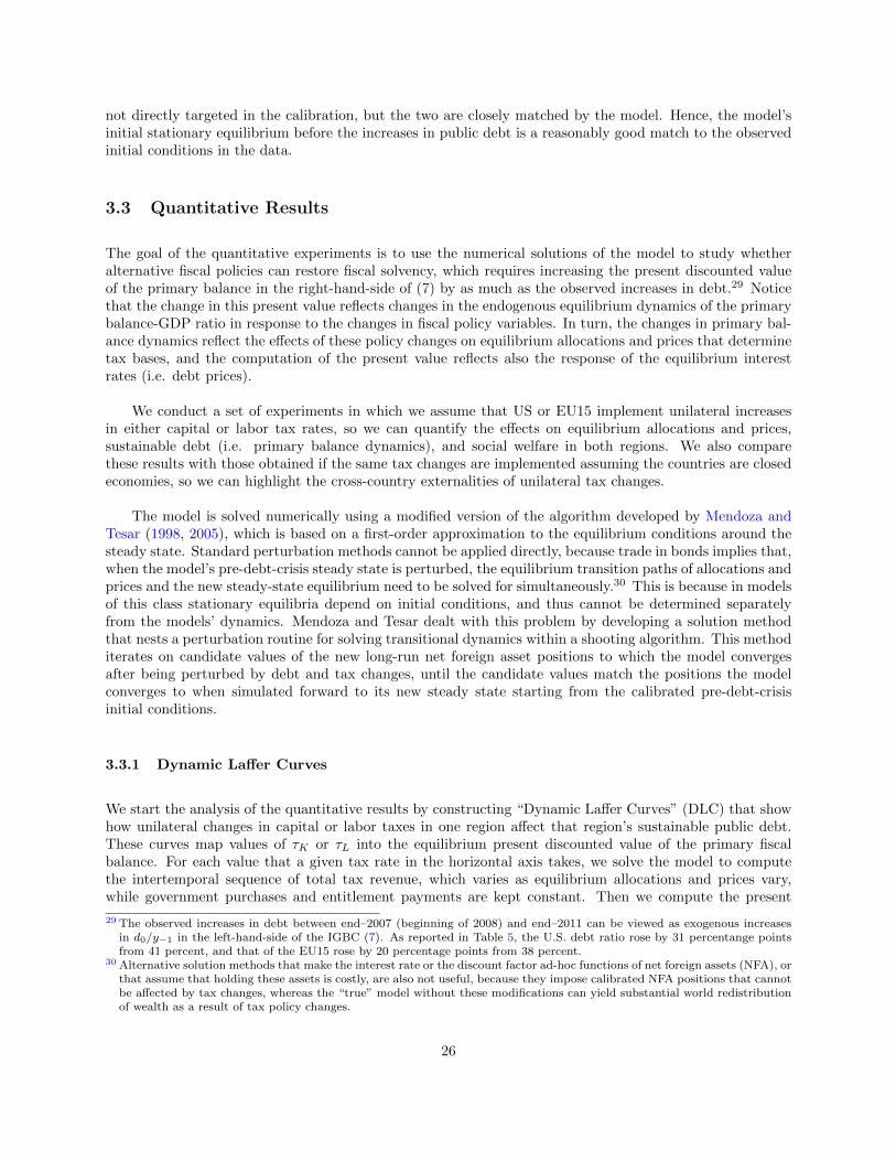
not directly targeted in the calibration, but the two are closely matched by the model. Hence, the model’sinitial stationary equilibrium before the increases in public debt is a reasonably good match to the observedinitial conditions in the data.

3.3 Quantitative Results

The goal of the quantitative experiments is to use the numerical solutions of the model to study whetheralternative fiscal policies can restore fiscal solvency, which requires increasing the present discounted valueof the primary balance in the right-hand-side of (7) by as much as the observed increases in debt.29 Noticethat the change in this present value reflects changes in the endogenous equilibrium dynamics of the primarybalance-GDP ratio in response to the changes in fiscal policy variables. In turn, the changes in primary bal-ance dynamics reflect the effects of these policy changes on equilibrium allocations and prices that determinetax bases, and the computation of the present value reflects also the response of the equilibrium interestrates (i.e. debt prices).

We conduct a set of experiments in which we assume that US or EU15 implement unilateral increasesin either capital or labor tax rates, so we can quantify the effects on equilibrium allocations and prices,sustainable debt (i.e. primary balance dynamics), and social welfare in both regions. We also comparethese results with those obtained if the same tax changes are implemented assuming the countries are closedeconomies, so we can highlight the cross-country externalities of unilateral tax changes.

The model is solved numerically using a modified version of the algorithm developed by Mendoza andTesar (1998, 2005), which is based on a first-order approximation to the equilibrium conditions around thesteady state. Standard perturbation methods cannot be applied directly, because trade in bonds implies that,when the model’s pre-debt-crisis steady state is perturbed, the equilibrium transition paths of allocations andprices and the new steady-state equilibrium need to be solved for simultaneously.30 This is because in modelsof this class stationary equilibria depend on initial conditions, and thus cannot be determined separatelyfrom the models’ dynamics. Mendoza and Tesar dealt with this problem by developing a solution methodthat nests a perturbation routine for solving transitional dynamics within a shooting algorithm. This methoditerates on candidate values of the new long-run net foreign asset positions to which the model convergesafter being perturbed by debt and tax changes, until the candidate values match the positions the modelconverges to when simulated forward to its new steady state starting from the calibrated pre-debt-crisisinitial conditions.

3.3.1 Dynamic Laffer Curves

We start the analysis of the quantitative results by constructing “Dynamic Laffer Curves” (DLC) that showhow unilateral changes in capital or labor taxes in one region affect that region’s sustainable public debt.These curves map values of τK or τL into the equilibrium present discounted value of the primary fiscalbalance. For each value that a given tax rate in the horizontal axis takes, we solve the model to computethe intertemporal sequence of total tax revenue, which varies as equilibrium allocations and prices vary,while government purchases and entitlement payments are kept constant. Then we compute the present

29 The observed increases in debt between end–2007 (beginning of 2008) and end–2011 can be viewed as exogenous increasesin d0/y−1 in the left-hand-side of the IGBC (7). As reported in Table 5, the U.S. debt ratio rose by 31 percentange pointsfrom 41 percent, and that of the EU15 rose by 20 percentage points from 38 percent.

30 Alternative solution methods that make the interest rate or the discount factor ad-hoc functions of net foreign assets (NFA), orthat assume that holding these assets is costly, are also not useful, because they impose calibrated NFA positions that cannotbe affected by tax changes, whereas the “true” model without these modifications can yield substantial world redistributionof wealth as a result of tax policy changes.

26

value of the primary balance, which therefore captures the effect of changes in the equilibrium sequence ofinterest rates. We take the ratio of this present value to the initial output y−1 (i.e. GDP in the steady statecalibrated to pre-2008 data) so that it corresponds to the term in the right-hand-side of the IGBC (7), andplot the result as a change relative to the 2007 public debt ratio. Hence, the values along the vertical axisof the DLCs show the change in d0/y−1 that particular values of τK or τL can support as sustainable debtat equilibrium (i.e. debt that satisfies the IGBC with equality). By construction, the curves cross the zeroline at the calibrated tax rates of the initial stationary equilibrium, because those tax rates yield exactlythe same present discounted value of the primary balance as the initial calibration. To make the observeddebt increases sustainable, there needs to be a value of the tax rate in the horizontal axis such that the DLCreturns a value in the vertical axis that matches the observed change in debt.

Since the “passive” region whose taxes are not being changed unilaterally is affected by spillovers of theother region’s tax changes, there needs be an adjustment in the passive region so that its IGBC is unchanged(i.e. it maintains the same present discounted value of primary fiscal balances). We refer to this adjustmentas maintaining “revenue neutrality” in the passive region. In principle this can be done by changing transfers,taxes or government purchases. However, since we have assumed already that government purchases are keptconstant in both regions, reducing distortionary tax rates in response to favorable tax spillovers would bemore desirable than increasing transfer payments, which are non-distortionary. Hence, we maintain revenueneutrality in the passive region by adjusting the labor tax rate.

Dynamic Laffer Curves for Capital Taxes

The DLCs for capital taxes are plotted in Figure 8. The left panel is for the US region, and the rightpanel is for EU15. The solid lines show the open-economy curves and the dotted lines are for when thecountries are in autarky. As explained above, the DLCs intersect the zero line at the initial tax rates ofτK = 0.37 and τ∗K = 0.32 by construction. We also show in the plots the increases in debt observed in eachregion, as shown in Table 5: The US net public debt ratio rose 31 percentage points and that of the EU15rose 20 percentage points. These increases are marked with the “Debt Shock” line in Figure 8.

Figure 8: Dynamic Laffer Curves of Capital Tax Rates

0.35 0.4 0.45 0.5

−0.2

−0.1

0

0.1

0.2

0.3

Capital Tax Rate

ΔPV

(Prim

ary

Bal

ance

)/y0

OpenClosed

Debt Shock

Pre−crisisTax Rate

Open Max

Closed Max

Debt Shock

Pre−crisisTax Rate

Open Max

Closed Max

(a) US

Capital Tax Rate0.15 0.2 0.25 0.3 0.35

ΔP

V(P

rimar

y B

alan

ce)/

y0

-0.3

-0.2

-0.1

0

0.1

0.2

0.3

0.4OpenClosed

Debt Shock

Pre-crisisTax Rate

Open Max

Closed Max

(b) EU15

Figure 8 shows that the DLCs of US and EU15 are very different, with those for EU15 seating higher,shifted to the left, and showing more curvature than those for US. Hence, unilateral changes in capital tax

27

rates show a capacity to sustain larger debt increases in EU15 than in US, and can do so at lower taxrates. These marked differences are the result of the heterogeneity in fiscal policies present in the dataand captured in the calibration, and in the open-economy scenario they are also partly explained by theinternational externalities of the unilateral tax changes assumed in constructing the DLCs. EU15 has higherrevenue-generating capacity because of higher labor and consumption taxes at identical labor income sharesand similar consumption shares, although in terms of primary balance the higher revenue is partly offset byhigher government purchases. On the other hand, US has a lower capital tax rate and by enough to makea significant difference in the inefficiencies created by capital taxes across the two regions, as we illustratein more detail below. Moreover, the magnitude of heterogeneity in the capital tax DLCs that results froma given magnitude of heterogeneity in fiscal variables depends on the model’s modifications made to matchthe observed elasticity of the capital base. We illustrate below that DLCs are very different if we removecapacity utilization and the limited depreciation allowance.

Beyond the difference in position and shape of the capital tax DLCs across US and EU15, these DLCsdeliver three striking results: First, unilateral changes in the US capital tax cannot restore fiscal solvencyand make the observed increase in debt unsustainable (the peaks of the DLCs of the US region either as aclosed or an open economy are significantly below the debt shock line). The maximum point of the open-economy DLC is attained at τK =0.402, which produces an increase in the present value of the primarybalance of only 2 percentage points of GDP, far short of the required 31. In contrast, the maximum point ofthe open-economy DLC for EU15 is attained around τ∗K =0.21, which rises the present value of the primarybalance by 22 percentage points of GDP, slightly more than the required 20. Under autarky, however, theEU15 DLC also peaks below the required level, and hence capital taxes also cannot restore fiscal solvencyfor EU15 as a closed economy. This result also reflects the strong cross-country externalities that we discussin more detail below (i.e. unilateral capital tax cuts yield significantly more sustainable debt for EU15 asan open economy than under autarky).

Second, capital income taxes in EU15 are highly inefficient. The current capital tax rate is on theincreasing segment of the DLC for US but on the decreasing segment for EU15. This has two importantimplications. One is that EU15 could have sustained the calibrated initial debt ratio of 38 percent at capitaltaxes below 15 percent, instead of the 32 percent tax rate obtained from the data. The second is that tomake the observed 20 percentage points increase in debt sustainable, EU15 can reduce its capital tax almostin half to about 17 percent in the open-economy DLC. In both cases, the sharply lower capital taxes wouldbe much less distortionary and thus would increase efficiency significantly.

Third, cross-country externalities of capital income taxes are very strong, and under our baseline cali-bration, they hurt (favor) the capacity to sustain debt of US (EU15). For US, the DLC under autarky issteeper than in the open-economy case, and it peaks at a higher tax rate of 43 percent and with a higherincrease in the present value of the primary balance of about 10 percentage points. Thus, US can alwayssustain more debt, or support higher debt increases relative to the calibrated baseline, for a given increasein τK under autarky than as an open economy. This occurs because by increasing its capital tax unilaterallyas an open economy the US not only suffers the efficiency losses in capital accumulation and utilization, butit also triggers reallocation of physical capital from US to EU15, which results in reductions (increases) inUS (EU15) factor payments and consumption, and thus lower (higher) tax bases in US (EU15). The samemechanism explains why reducing the capital tax in the EU15 unilaterally generates much less revenue underautarky than in the open-economy case. In the latter, cutting the EU15 capital tax unilaterally triggers thesame forces as a unilateral increase in the US capital tax.

This quantitative evidence of strong externalities of capital taxes across financially integrated economiesdemonstrates that evaluating “fiscal space,” or the capacity to sustain debt, using closed-economy modelsleads to seriously flawed estimates of the effectiveness of capital taxes as a tool to restore debt sustainability.The results also suggest that incentives for strategic interaction leading to capital income tax competition are

28

strong, and get stronger as higher debts need to be reconciled with fiscal solvency (as evidenced by the historyof corporate tax competition inside the EU since the 1980s). Mendoza, Tesar, and Zhang (2014) study thisissue using a calibration that splits the European Union into two regions, one including the countries mostaffected by the European debt crisis (Greece, Ireland, Italy, Portugal and Spain) and the second includingthe rest of the Eurozone members.

Dynamic Laffer Curves of Labor Tax Rates

Figure 9 shows the DLCs for the labor tax rate. Notice that the open-economy and autarky DLCs aresimilar within each region (although more similar for EU15 than for US), which indicates that internationalexternalities are much weaker in this case. This is natural, because labor is an immobile factor, and althoughit can still trigger cross-country spillovers via general-equilibrium effects, these are much weaker than thefirst-order effects created by unilateral changes of capital taxes via the condition that arbitrages after-taxreturns on all assets across countries.

The main result of the DLCs for labor taxes is that the DLCs for US are much higher than those for theEU15. Since the international externalities are weak for the labor tax, this result is only due to the differentinitial conditions resulting from the fiscal heterogeneity captured in our calibration, and in particular to thelarge differences in initial labor and consumption taxes (41 v. 27 percent for labor and 17 v. 4 percentfor consumption in the EU15 v. US respectively). Increasing the calibrated τL for the US region to theEU15 rate of 41 percent, keeping all other US parameters unchanged, shifts down its labor tax DLC almostuniformly by about 200 percentage points in the 0.25-0.55 interval of labor tax rates. This happens because,for an increase in the labor tax of a given size, the difference in initial conditions implies that the US regiongenerates a larger increase in the present value of total tax revenue than EU15, and since the present valueof government outlays is nearly unchanged in both, the larger present value of revenue is amplified into asignificantly larger increase in the present value of the primary balance.31

The US open-economy DLC for τL is considerably steeper than for τK , and it peaks at a tax rate of0.48, which would make sustainable an initial debt ratio larger than in the initial baseline by 200 percentagepoints of GDP, much more than the 31 percentage points required by the data. The labor tax rate thatUS as an open or closed economy needs to make the observed debt increase sustainable is about 29 percent,which is just a two-percentage-point increase relative to the initial tax rate. Hence, these results show that,from the perspective of macroeconomic efficiency that representative-agent models of financially-integratedeconomies like the one we are using emphasize, labor taxes are a significantly more effective tool for restoringfiscal solvency in the United States than capital taxes.

The DLC of the EU15 yields much less positive results. Since the initial consumption-labor wedge isalready much higher in this region than in US, the fiscal space of the labor tax rate is very limited. Ineither the closed- or open-economy cases, the DLC peaks at a labor tax rate of 46 percent and yields anincrease of only about 10 percentage points in the present value of the primary balance, which is half of the20-percentage-points increase EU15 needs make the observed debt increase sustainable.

It is interesting to note that the debt increase in the United States was about 10 percentage points largerthan in Europe, yet the model predicts that given the initial conditions in tax rates and government outlaysbefore the increases in debt, unilateral tax adjustments in Europe cannot generate a sufficient increase in

31 The percent change in the present value of the primary balance after a tax change of a given magnitude relative to before(assuming that the present value of government outlays does not change) can be expressed as z[1 + PDV (g + e)/PDV (pb)],where z is the percent change in the present value of tax revenues after the tax change relative to before, and PDV (g +e) and PDV (pb) are the pre-tax-change present values of total government outlays and the primary balance respectively.Hence, for z > 0 and since total outlays are much larger than the primary balance [PDV (g + e)/PDV (pb)] >> 1, a givendifference in z across US and EU15 translates into a much larger percent difference in the present value of the primarybalance.

29

Figure 9: Dynamic Laffer Curves of Labor Tax Rates

0.25 0.3 0.35 0.4 0.45 0.5 0.55 0.6−1.5

−1

−0.5

0

0.5

1

1.5

2

2.5

Labor Tax Rate

ΔPV

(Prim

ary

Bal

ance

)/y0

OpenClosedDebt Shock

Pre−crisisTax Rate

Open Max

Closed Max

(a) US

Labor Tax Rate0.3 0.35 0.4 0.45 0.5 0.55

ΔP

V(P

rimar

y B

alan

ce)/

y0

-1.5

-1

-0.5

0

0.5OpenClosed

Debt Shock

Pre-crisisTax Rate

Open Max

Closed Max

(b) EU15

the present value of the primary balance to make their higher debt sustainable. The exception is the capitaltax in the open-economy scenario, in which this is possible only because EU15 would benefit significantlyfrom a negative externality on the US region. In contrast, the results show that a modest increase in labortaxes (or consumption taxes since they are equivalent in this model) can restore fiscal solvency in the UnitedStates.

It is useful to compare the results we reported here with those of similar exercises in other existing studiesbased on Neoclassical models, particularly those by Trabandt and Uhlig (2011, 2012) and Auray, Eyquem,and Gomme (2013). Trabandt and Uhlig (2011, 2012) used a closed-economy model without endogenouscapacity utilization and focused mainly on steady-state Laffer curves (i.e. Laffer curves that map tax ratesinto steady state tax revenues), while the DLCs studied here are for present values taking into account bothtransitional dynamics and steady-state changes caused by tax changes relative to the calibrated tax rates.Qualitatively, the results in Trabandt and Uhlig (2011) are similar to the ones in this Chapter because theyfind that capital tax hikes generate much smaller increases in revenue than labor taxes. They find that themaximum increases in steady-state tax revenue obtained with capital (labor) taxes are 6 (30) percent for theUnited States and 1 (8) percent for Europe. Quantitatively, however, the results reported here differ not onlybecause both transitional dynamics and steady-states are included, but also because the two-country modelwith capacity utilization captures the cross-country externalities of tax policy and the observed elasticity ofthe capital tax base, and these two features undermine the revenue-generating capacity of tax hikes.

Trabandt and Uhlig (2012) extend their analysis to gauge the sustainability of observed debt levelsin response to hypothetical permanent increases in interest rates. Keeping government transfers, totaloutlays and debt constant at observed levels, they calculate the maximum real interest rate at which therevenue generated at the peak of steady-state Laffer curves would satisfy the steady-state government budgetconstraint. That is, effectively they compute the interest rate at which the Blanchard ratio of the previousSection holds with debt and spending set at observed levels and tax revenue set at the maxima of steady-state Laffer curves. They find that the maximum real interest rate for the United States is larger than forEuropean countries if labor taxes are moved to the peak of the Laffer curves. These calculations, however,inherit the limitations of the Blanchard ratios as measures of sustainable debt discussed in the previousSection, and imply unusually large primary fiscal surpluses. For instance, depending on the debt measure

30

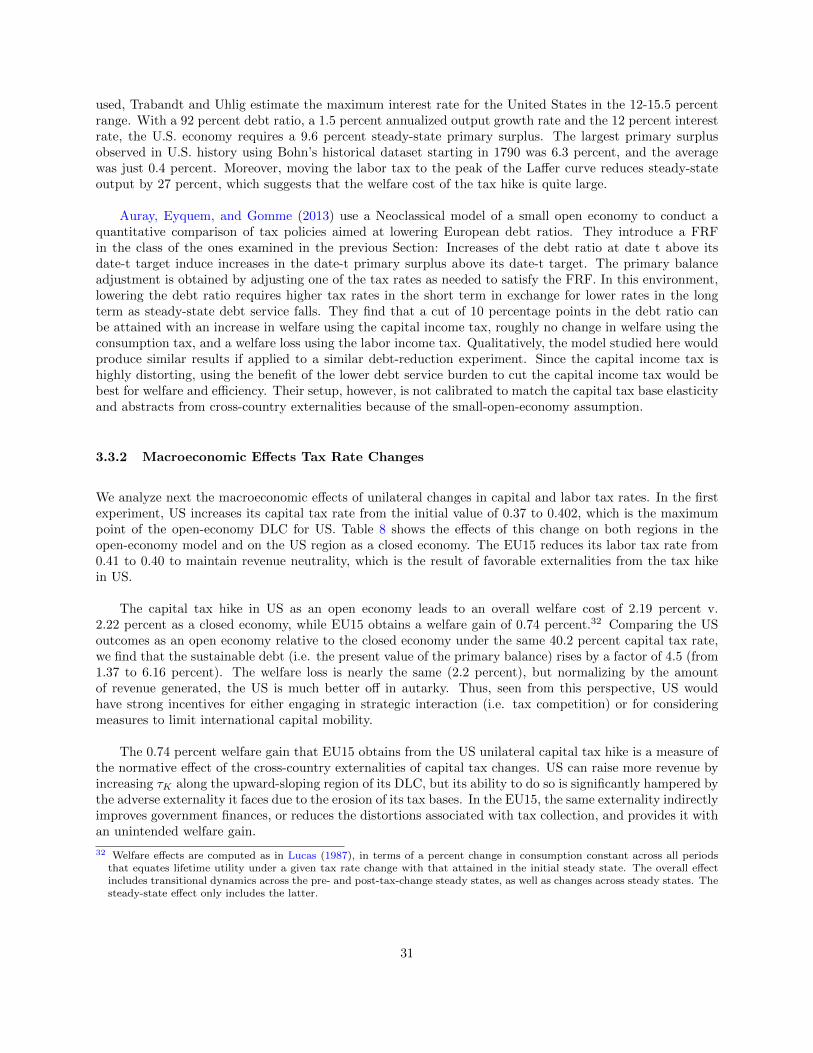
used, Trabandt and Uhlig estimate the maximum interest rate for the United States in the 12-15.5 percentrange. With a 92 percent debt ratio, a 1.5 percent annualized output growth rate and the 12 percent interestrate, the U.S. economy requires a 9.6 percent steady-state primary surplus. The largest primary surplusobserved in U.S. history using Bohn’s historical dataset starting in 1790 was 6.3 percent, and the averagewas just 0.4 percent. Moreover, moving the labor tax to the peak of the Laffer curve reduces steady-stateoutput by 27 percent, which suggests that the welfare cost of the tax hike is quite large.

Auray, Eyquem, and Gomme (2013) use a Neoclassical model of a small open economy to conduct aquantitative comparison of tax policies aimed at lowering European debt ratios. They introduce a FRFin the class of the ones examined in the previous Section: Increases of the debt ratio at date t above itsdate-t target induce increases in the date-t primary surplus above its date-t target. The primary balanceadjustment is obtained by adjusting one of the tax rates as needed to satisfy the FRF. In this environment,lowering the debt ratio requires higher tax rates in the short term in exchange for lower rates in the longterm as steady-state debt service falls. They find that a cut of 10 percentage points in the debt ratio canbe attained with an increase in welfare using the capital income tax, roughly no change in welfare using theconsumption tax, and a welfare loss using the labor income tax. Qualitatively, the model studied here wouldproduce similar results if applied to a similar debt-reduction experiment. Since the capital income tax ishighly distorting, using the benefit of the lower debt service burden to cut the capital income tax would bebest for welfare and efficiency. Their setup, however, is not calibrated to match the capital tax base elasticityand abstracts from cross-country externalities because of the small-open-economy assumption.

3.3.2 Macroeconomic Effects Tax Rate Changes

We analyze next the macroeconomic effects of unilateral changes in capital and labor tax rates. In the firstexperiment, US increases its capital tax rate from the initial value of 0.37 to 0.402, which is the maximumpoint of the open-economy DLC for US. Table 8 shows the effects of this change on both regions in theopen-economy model and on the US region as a closed economy. The EU15 reduces its labor tax rate from0.41 to 0.40 to maintain revenue neutrality, which is the result of favorable externalities from the tax hikein US.

The capital tax hike in US as an open economy leads to an overall welfare cost of 2.19 percent v.2.22 percent as a closed economy, while EU15 obtains a welfare gain of 0.74 percent.32 Comparing the USoutcomes as an open economy relative to the closed economy under the same 40.2 percent capital tax rate,we find that the sustainable debt (i.e. the present value of the primary balance) rises by a factor of 4.5 (from1.37 to 6.16 percent). The welfare loss is nearly the same (2.2 percent), but normalizing by the amountof revenue generated, the US is much better off in autarky. Thus, seen from this perspective, US wouldhave strong incentives for either engaging in strategic interaction (i.e. tax competition) or for consideringmeasures to limit international capital mobility.

The 0.74 percent welfare gain that EU15 obtains from the US unilateral capital tax hike is a measure ofthe normative effect of the cross-country externalities of capital tax changes. US can raise more revenue byincreasing τK along the upward-sloping region of its DLC, but its ability to do so is significantly hampered bythe adverse externality it faces due to the erosion of its tax bases. In the EU15, the same externality indirectlyimproves government finances, or reduces the distortions associated with tax collection, and provides it withan unintended welfare gain.

32 Welfare effects are computed as in Lucas (1987), in terms of a percent change in consumption constant across all periodsthat equates lifetime utility under a given tax rate change with that attained in the initial steady state. The overall effectincludes transitional dynamics across the pre- and post-tax-change steady states, as well as changes across steady states. Thesteady-state effect only includes the latter.

31

The impact and long-run effects on key macro-aggregates in both regions are shown in the bottom halfof Table 8. The corresponding transition paths of macroeconomic variables as the economies move from thepre-crisis steady state to the new steady state are illustrated in Figure 10. The increase in τK causes UScapital to fall over time to a level 7.6 percent below the pre-crisis level, while EU15’s capital rises to a level1.25 percent above the pre-tax-change level. Capacity utilization falls at home in both the short run andthe long run, which is a key component of the model capturing the reduced revenue-generating capacity ofcapital tax hikes when the endogeneity of capacity utilization is considered. We show later in this sectionthat this mechanism indeed drives the elasticity of the capital tax base in the model, which matches that ofthe data and is higher than what standard representative-agent models of taxation show.

Figure 10: Responses of Macro Variables to a US Capital Tax Rate Increase

0 50 100-5

0

5Consumption

US Open EU15 Open US Closed

0 20 40 60 80 100-4

-2

0

2Utility

0 50 100-5

0

5GDP

0 50 100-10

0

10Capital Stock

0 50 100-0.5

0

0.5Labor

0 50 100-10

-5

0Utilization

0 50 100-5

0

5TB over GDP

0 50 100

×10-4

-4

-2

0Interest Rate

On impact when US increases its capital tax, labor increases in US and falls slightly in EU15, butthis pattern reverses during the transition to steady state because of the lower (higher) capital stock inUS (EU15) region in the new steady state. Consequently, US output contracts by almost 4 percent in thelong-run, underscoring efficiency losses due to the capital tax increase and the costs of the fiscal adjustment.US increases its net foreign asset position (NFA) by running trade surpluses (tb/y) in the early stages oftransition, while EU15 decreases its NFA position by running trade deficits. The US trade surpluses reflectsaving to smooth out the cost of the efficiency losses, as output follows a monotonically decreasing path.Still, utility levels are lower than when US implements the same capital tax under autarky, because of thenegative cross-country spillovers.

We next look at the responses of fiscal variables when US increases its capital tax, plotted in Figure11. In the U.S., tax revenue from capital income increases almost immediately to a higher constant levelwhen τk rises, while the revenues from labor and consumption taxes decline both on impact and in thelong run. Labor and consumption tax rates are not changing, but both tax bases fall on impact and thendecline monotonically to their new, lower steady states. The primary fiscal balance and total revenue bothrise initially but then converge to about the same levels as in the pre-crisis stationary equilibrium. For theprimary balance, this pattern is implied by the pattern of the total revenue, since government expendituresand entitlements are held constant. For total revenue, the transitional increase indicates that the rise incapital tax revenue more than offsets the decline in the revenue from the other taxes in the transition, whilein the long-run they almost offset each other exactly. This is possible because the change in τK to 0.4 is on

32

the increasing side of the Laffer curve, and in fact it is the maximum point of the curve. Hence, this capitaltax hike does not reduce capital tax revenues.

Figure 11: Responses of Fiscal Variables to a US Capital Tax Rate Increase

0 50 100

×10-3

-5

0

5Total Revenue

US Open EU15 Open US Closed

0 50 100

×10-3

-5

0

5

10=

k Revenue

0 50 100

×10-3

-6

-4

-2

0=

n Revenue

0 50 100

×10-3

-1

0

1

2=

c Revenue

0 50 100

×10-3

-5

0

5Primary Fiscal Balance

0 50 100-0.1

0

0.1

0.2

Govt Debt over y0

The public debt dynamics in the bottom-right panel of Figure 11 shows that on impact, governmentdebt in the U.S. responds to the 40 percent tax rate by increasing 5 percentage points, reflecting the extrainitial debt that can be supported at the higher capital tax rate. Since the primary fiscal balance rises onimpact and then declines monotonically, the debt ratio also falls monotonically during the transition, andconverges to a ratio that is actually about 4 percentage points below the pre-crisis level. Hence, the initialdebt increase allowed by the capital tax hike is followed by a protracted decline in debt converging to adebt ratio even lower that in the pre-crisis steady state. If the U.S. implements the same tax hike underautarky, it generates significantly larger revenues and primary balances, and hence the debt ratio increasesmore initially and converges to a higher steady state of 1 percentage points above the pre-crisis level. This isagain a reflection of the cross-country externalities faced by the U.S. as an open economy, since equally-sizedtax hikes produce significantly higher revenues under autarky.

The cross-country externalities are also reflected in the fiscal dynamics of the EU15 shown in Figure 11.Maintaining revenue neutrality (in present value) still allows both its revenue and primary balance to fallinitially, while in the long run both converge to very similar levels as in the pre-crisis steady state. Removingthe labor tax adjustment in the EU15 that maintains revenue neutrality, the present value of its primarybalance as a share of GDP would increase by 10.1 percentage points relative to the pre-crisis ratio, and bothits revenue and primary balances would be higher than in the plots shown in Figure 11. The welfare gain,however, would be negligible instead of 0.74 percent in lifetime consumption.

The next experiment examines the effects of lowering the EU15 capital tax rate so as to move it out ofthe decreasing segment of the DLC. To make this change analogous to the one in the previous experiment,we change the EU15 capital tax to the value at the maximum point of the DLC for EU15, which is about21 percent. Table 9 summarizes the results. The cut in the EU15 capital tax rate generates an increase ofabout 22 percentage points in sustainable debt (just a notch above what is required to make the observeddebt increase sustainable), and a large welfare gain of 6.9 percent for this region. Its capital stock risesover time to a level 26 percent higher than in the pre-tax-change steady state. Output, consumption, labor

33

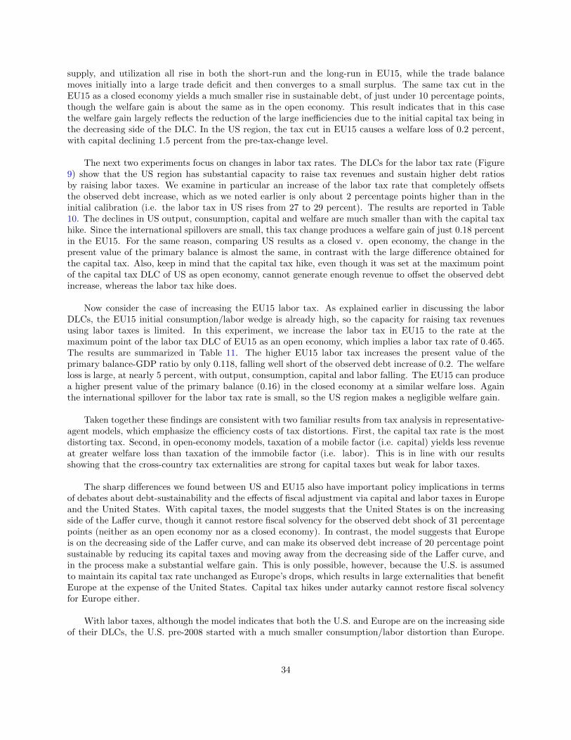
supply, and utilization all rise in both the short-run and the long-run in EU15, while the trade balancemoves initially into a large trade deficit and then converges to a small surplus. The same tax cut in theEU15 as a closed economy yields a much smaller rise in sustainable debt, of just under 10 percentage points,though the welfare gain is about the same as in the open economy. This result indicates that in this casethe welfare gain largely reflects the reduction of the large inefficiencies due to the initial capital tax being inthe decreasing side of the DLC. In the US region, the tax cut in EU15 causes a welfare loss of 0.2 percent,with capital declining 1.5 percent from the pre-tax-change level.

The next two experiments focus on changes in labor tax rates. The DLCs for the labor tax rate (Figure9) show that the US region has substantial capacity to raise tax revenues and sustain higher debt ratiosby raising labor taxes. We examine in particular an increase of the labor tax rate that completely offsetsthe observed debt increase, which as we noted earlier is only about 2 percentage points higher than in theinitial calibration (i.e. the labor tax in US rises from 27 to 29 percent). The results are reported in Table10. The declines in US output, consumption, capital and welfare are much smaller than with the capital taxhike. Since the international spillovers are small, this tax change produces a welfare gain of just 0.18 percentin the EU15. For the same reason, comparing US results as a closed v. open economy, the change in thepresent value of the primary balance is almost the same, in contrast with the large difference obtained forthe capital tax. Also, keep in mind that the capital tax hike, even though it was set at the maximum pointof the capital tax DLC of US as open economy, cannot generate enough revenue to offset the observed debtincrease, whereas the labor tax hike does.

Now consider the case of increasing the EU15 labor tax. As explained earlier in discussing the laborDLCs, the EU15 initial consumption/labor wedge is already high, so the capacity for raising tax revenuesusing labor taxes is limited. In this experiment, we increase the labor tax in EU15 to the rate at themaximum point of the labor tax DLC of EU15 as an open economy, which implies a labor tax rate of 0.465.The results are summarized in Table 11. The higher EU15 labor tax increases the present value of theprimary balance-GDP ratio by only 0.118, falling well short of the observed debt increase of 0.2. The welfareloss is large, at nearly 5 percent, with output, consumption, capital and labor falling. The EU15 can producea higher present value of the primary balance (0.16) in the closed economy at a similar welfare loss. Againthe international spillover for the labor tax rate is small, so the US region makes a negligible welfare gain.

Taken together these findings are consistent with two familiar results from tax analysis in representative-agent models, which emphasize the efficiency costs of tax distortions. First, the capital tax rate is the mostdistorting tax. Second, in open-economy models, taxation of a mobile factor (i.e. capital) yields less revenueat greater welfare loss than taxation of the immobile factor (i.e. labor). This is in line with our resultsshowing that the cross-country tax externalities are strong for capital taxes but weak for labor taxes.

The sharp differences we found between US and EU15 also have important policy implications in termsof debates about debt-sustainability and the effects of fiscal adjustment via capital and labor taxes in Europeand the United States. With capital taxes, the model suggests that the United States is on the increasingside of the Laffer curve, though it cannot restore fiscal solvency for the observed debt shock of 31 percentagepoints (neither as an open economy nor as a closed economy). In contrast, the model suggests that Europeis on the decreasing side of the Laffer curve, and can make its observed debt increase of 20 percentage pointsustainable by reducing its capital taxes and moving away from the decreasing side of the Laffer curve, andin the process make a substantial welfare gain. This is only possible, however, because the U.S. is assumedto maintain its capital tax rate unchanged as Europe’s drops, which results in large externalities that benefitEurope at the expense of the United States. Capital tax hikes under autarky cannot restore fiscal solvencyfor Europe either.

With labor taxes, although the model indicates that both the U.S. and Europe are on the increasing sideof their DLCs, the U.S. pre-2008 started with a much smaller consumption/labor distortion than Europe.

34

As a result, the U.S. has substantial fiscal space to easily offset the debt increase with a small labor tax hikeand a small welfare cost of 0.9 percent. In contrast, the model suggests that Europe cannot restore fiscalsolvency after the observed increase in debt using labor taxes.

3.3.3 Why are Utilization and Limited Depreciation Allowance Important?

As explained earlier, we borrowed from Mendoza, Tesar, and Zhang (2014) the idea of using endogenouscapacity utilization and a limited tax allowance for depreciation expenses to build into the model a mechanismthat produces capital tax base elasticities in line with empirical estimates. In contrast, standard dynamicequilibrium models without these features tend to have unrealistically low responses of the capital base toincreases in capital taxes. To illustrate this point, we follow again Mendoza et al. in comparing DLCs forcapital taxes in three scenarios (see Figure 12): (i) a standard Neoclassical model with exogenous utilizationand a full depreciation allowance (θ = 1), shown as a dashed-dotted line; (ii) the same model but with alimited depreciation allowance (θ = 0.2), shown as a dotted line; and (iii) the baseline calibration of ourmodel with both endogenous utilization and a limited depreciation allowance (using again θ = 0.2), shownas a solid line. All other parameter values are kept the same. We show the three cases for the US and EU15region in panels (a) and (b) of the Figure respectively.

Figure 12: Comparing Dynamic Laffer Curves for the Capital Tax Rate

0.35 0.4 0.45 0.5

−0.2

−0.1

0

0.1

0.2

0.3

Capital Tax Rate

ΔPV

(Prim

ary

Bal

ance

)/y0

Endog UtilExog UtilExog Util θ=1

(a) US

0.1 0.15 0.2 0.25 0.3 0.35

−0.2

−0.1

0

0.1

0.2

0.3

Capital Tax Rate

ΔPV

(Prim

ary

Bal

ance

)/y0

Endog UtilExog UtilExog Util θ=1

(b) EU15

The DLCs for the three cases intersect at the initial calibrated tax rates of 0.37 and 0.32 for the US andEU15 by construction. To the right of this point, the curves for case (i) are always above the other two,and the ones for case (ii) are always above the ones for case (iii). The opposite occurs to the left of theintersection points.

Consider the US plots. In case (i), the DLC has a positive, approximately linear slope in the 0.35–0.5domain of capital tax rates. This curve continues to be increasing even when we extend the capital tax rateto 0.9, which is in line with the results obtained by Trabandt and Uhlig (2011).33 This behavior of the DLCfor the capital tax follows from the fact that at any given date the capital stock is predetermined and has alow short-run elasticity. As a result, the government can raise substantial revenue over the transition period

33 They find that present-value Laffer curves of capital tax revenue peak at very high tax rates (discounting with the constantsteady state interest rate) or have a positive slope over the full range (discounting with equilibrium interest rates).

35

because the capital stock declines only gradually. The increased tax revenue during the transition dominatesthe fall in the steady-state, resulting in a non-decreasing DLC (recall the DLC is based on present valuecalculations).

Introducing limited depreciation allowance without endogenizing the utilization choice (case (ii)) has twoeffects that induce concavity in the DLC. First, it increases the effective rate of taxation on capital income,and thus weakens the incentive to accumulate capital and lowers the steady-state capital-output ratio andtax bases. On the other hand, it has a positive impact on revenue by widening the capital tax base. Thefirst effect dominates the latter when the capital tax rate rises relative to the initial tax of 0.37, resulting insharply lower DLC curve values than in case (i).

In case (iii) the tax allowance is again limited but now capacity utilization is endogenous. This introducesadditional effects that operate via the distortions on efficiency and the ability to raise revenue discussedearlier: On the side of tax distortions, equation (9) implies that endogenous utilization adds to the efficiencycosts of capital income taxation by introducing a wedge between the marginal cost and benefits of capitalutilization. On the revenue side, endogenous utilization allows agents to make adjustments in effectivecapital (reducing it when taxes rise and increasing it when it falls), and thus alters the amount of taxablecapital income. Hence, when utilization falls in response to increases in capital tax rates, it also weakensthe government’s ability to raise capital tax revenue. These effects lead to a bell-shaped DLC that has morecurvature and is significantly below those in cases (i) and (ii). Thus, endogenous utilization makes capitaltaxes more distorting and weakens significantly the revenue-generating capacity of capital taxes.34

Panel (b) of Figure 12 shows DLCs for the three cases in the EU15 region. The results are analogous toPanel (a) but emphasizing now the region to the left of the intersection point, which is at the initial tax of 32percent. In case (i), again the DLC has an increasing positive slope over a large range of the capital tax rate.Case (ii) shows that limiting the depreciation allowance again induces concavity in the DLC, with the EU15initial capital tax already in the decreasing segment of the curve. Comparing with case (iii), the exogenousutilization case generates much less revenue. As in the US results, this occurs because with endogenousutilization, reductions in capital taxes lead to higher utilization rates that result in higher levels of capitalincome and higher wages, thus widening the two income tax bases.

The effects of endogenous utilization and limited depreciation have significant implications for the elas-ticity of the capital income tax base with respect to the capital tax. In particular, as Mendoza, Tesar, andZhang (2014) showed, the model can be calibrated to match a short-run elasticity consistent with empiricalestimates because of the combined effects of those two features. As documented earlier, the empirical litera-ture finds estimates of the short-run elasticity of the capital tax base in the 0.1–0.5 range. Table 12 reportsthe model’s comparable elasticity estimates and the effects on output, labor and utilization one year after a1-percent increase in the capital tax (relative to the calibrated baseline values), again for cases (i), (ii) and(iii) and in both US and EU15 regions.

The US and EU15 results differ somewhat quantitatively, but qualitatively they make identical points:The neoclassical model with or without limited depreciation allowance (cases (i) and (ii)) yields short-runelasticities with the wrong sign (i.e. the capital tax base rises in the short run in response to capital taxrate increases). The reason is that capital income does not change much, since capital is pre-determined inthe period of the tax hike and changes little in the first period after because of investment adjustment costs,and labor supply rises due to a negative income shock from the tax hike. Since capital does not fall muchand labor rises, output rises on impact, and thus taxable labor and capital income both rise, producing anelasticity of the opposite sign than that found in the data. In contrast, the model with endogenous utilization(case (iii)), generates a decline in output on impact due to a substantial drop in the utilization rate, despite

34 Mendoza et al. also found that removing the limited depreciation allowance from case (iii) still results in a DLC below thoseof cases (i) and (ii), but it is also flatter and increasing for a wider range of capital taxes than case (iii).

36

the rise in labor supply. With the calibrated values of η, the model generates short-run elasticities of 0.29and 0.32 for US and EU15 respectivelye, which are both well inside the range of empirical estimates.

It is also worth noting that with exogenous utilization, the model can produce a capital tax base elasticityin line with empirical evidence only if we set η to an unrealistically low value. The short-run elasticity of thecapital tax base is negative for any η > 1, and it becomes positive and higher than 0.1 only for η < 0.1.35

This is significantly below the empirically relevant range of 1–2.5 documented in the calibration section.Moreover, at the value of η = 2 determined in our baseline calibration, the model without utilization choiceyields a capital tax base elasticity of −0.09.

3.3.4 Further Considerations

We close this Section with some important considerations and caveats of the structural analysis. In particular,we discuss the predictions of the structural framework for the case of Japan, which is challenging because ofits high debt ratio, and the implications of considering the possibility of taxes on wealth or the capital stock.

Japan had a very high public debt to GDP ratio already before the global financial crisis, at about 82percent by the end of 2007. By the end of 2011, its debt ratio had increased 46 percentage points to 128percent. Hence the level and the change of Japan’s debt ratio are both larger than what we saw in the U.S.and Europe.

What does the structural approach to debt sustainability tell us about the Japanese case? To answerthis question, we reset the model so that the foreign region is now a proxy for Japan instead of the EU15and recompute the DLCs. In particular, we calibrate the foreign tax rates to match Japan’s pre-crisis taxstructure, using the same Mendoza-Razin-Tesar method we used for the U.S. and Europe. In 2007, Japan’scapital tax rate was 39 percent, the labor tax rate was 31 percent and the consumption tax was 6 percent.This tax structure is similar to that of the United States. In fact, Japan’s consumption-leisure tax wedge τWis 0.35, which is much closer to the 0.3 estimate for the U.S. than 0.5 for Europe. We also reset the relativecountry size to match the fact that Japan’s GDP per capita is about 78 percent that of the United States.The rest of the structural parameters are kept the same as in our baseline analysis. The DLCs for Japan areshown in Figure (13). The left panel is the DLC for the capital tax and the right panel is for the labor tax.

In general, the DLC results for Japan are a more extreme version of those for the United States: Thecapital tax cannot restore fiscal solvency because Japan’s DLC for this tax peaks well below the requiredincrease, while there is a lot of room for labor (or consumption) taxes to do it. One important difference isthat the pre-crisis high capital tax rate in Japan is inefficient (i.e. in the decreasing segment of the DLC).Because of this, the tax externalities work in the opposite direction to those observed for the US DLC, andso cutting the capital tax in Japan relative to the pre-crisis rate as a closed economy yields a smaller increasein the present value of the primary balance than as an open economy.

One important caveat to the above results is that Japan has been stuck with slow growth and deflationfor about two decades. Although raising consumption and labor taxes helps balance government budgets,higher taxes still cause efficiency and welfare losses. Japan did increase its consumption tax from 5 to8 percent in April 2014, but after that the economy tipped back into recession and a further hike of theconsumption tax to 10 percent was postponed. Moreover, if we reduce the long-run growth rate in the modelto the 0.8 percent per-capita GDP growth rate observed on average in Japan between 2001 and 2014, thetwo DLCs shift downward sharply. The capital tax becomes effectively useless as it yields negligible amounts

35 The intuition is simple. As η approaches zero the marginal adjustment cost of investment approaches zero, and hence thecapital stock one year after the tax hike can respond with large declines.

37

Figure 13: Dynamic Laffer Curves for Japan

Capital Tax Rate0.3 0.35 0.4 0.45

∆PV

(Prim

ary

Bala

nce)

/y0

-0.5

-0.4

-0.3

-0.2

-0.1

0

0.1

0.2

0.3

0.4

0.5OpenClosed

Debt Shock

Pre-crisisTax Rate

Open Max

Closed Max

(a) Capital Tax

Labor Tax Rate0.3 0.35 0.4 0.45 0.5 0.55 0.6

∆PV

(Prim

ary

Bala

nce)

/y0

-1.5

-1

-0.5

0

0.5

1

1.5

2

2.5

3OpenClosed

Debt Shock

Pre-crisisTax Rate

Open Max

Closed Max

Debt Shock

Pre-crisisTax Rate

Open Max

Closed Max

Debt Shock

Pre-crisisTax Rate

Open Max

Closed Max

Debt Shock

Pre-crisisTax Rate

Open Max

Closed Max

Debt Shock

Pre-crisisTax Rate

Open Max

Closed Max

(b) Labor Tax

of extra revenue. The labor tax needed to make the debt sustainable is significantly higher, and thus theassociated efficiency and welfare losses are larger as well.

Another caveat is that our analysis abstracts from Japan’s aging demographics, rising pressures ongovernment finance from public pensions and medical expenses, etc. These considerations place heavyburdens on the sustainability of public debt. Imrohoroglu and Sudo (2011) and Hansen and Imrohoroglu(2013) use a Neoclassical growth model to quantify the implications of the projected low population growthrate and permanent increase in total government outlays on fiscal sustainability. Imrohoroglu and Sudo findthat even an increase in the consumption tax to 15 percent and an annual GDP growth of 3 percent over thenext 20 years is not sufficient to restore fiscal balance unless expenditures are also contained. Hansen andImrohoroglu find that fiscal sustainability requires the consumption tax rate be set to unprecedentedly highlevels of 40-60 percent. Moreover, Imrohoroglu, Kirao, and Yamada (2016) and Braun and Joines (2015) useoverlapping generation models and also find that current fiscal policies are not sustainable and large fiscaladjustments are needed.36

Another important consideration in assessing the results of the structural analysis is that we abstractedfrom the possibility of taxing wealth, in particular taxing the initial capital stock. The optimal taxation liter-ature has made the well-known argument that from an efficiency standpoint taxing the initial, pre-determinedcapital stock is optimal. However, the argument hinges on the assumption of government commitment, whichsets aside key issues of time consistency and the implications of lack of commitment.

In our model, a wealth tax would be equivalent to confiscation of a fraction of K0 unexpectedly. Sinceutilization is endogenous, this tax would also affect utilization as of date 0: The marginal product of utiliza-tion declines with lower capital, utilization falls, and thus capital income and capital income tax revenue fall.But more importantly, three arguments raise serious questions about the possibility of taxing wealth in thisway. First, the government would have to sell confiscated capital to raise revenue (in the realistic scenario inwhich confiscated capital and government outlays involve different goods and services), which would lowerthe price at which capital goods can be sold. Second, the expectation of future confiscation of capital wouldnot be zero, and to the extent that is positive it would act as a tax on future capital accumulation and

36 In the next Section we discuss the implications of unfunded pension and entitlement liabilities for debt sustainability whenthe government is not committed to repay and responds to distributional incentives to default.

38

capital income. Third, as an implication of the first two arguments, the wealth tax actually looks more likea government default that would seem to necessitate modeling government behavior without commitment(in fact, in a setup without utilization and capital as the only productive factor, the government confiscatingsome of K0 is equivalent to defaulting on a fraction of the date-0 debt repayment).

Perhaps because of the above arguments, the history of wealth taxes has not been a happy one. Wealthtaxes were discarded by Austria, Denmark and Germany in 1997, by Finland, Iceland and Luxembourgin 2006 and by Sweden in 2007. Interestingly, these countries claimed to ditch the wealth tax in effortsto get more revenue, not less. Moreover, implementing wealth taxation faces serious hurdles, particularlyfor the valuation of assets and for preventing tax evasion. Global financial integration also makes taxingwealth more difficult, because the expectation of potential future confiscation via wealth taxes mentionedabove discourages investment and encourages capital flight (see the discussion in Eichengreen (1989) and therecent experience with “tax inversions” in the United States).

To summarize where the Chapter is at this point, we first explored the question of public debt sustain-ability from the viewpoint of an empirical approach based on the estimation and analysis of fiscal reactionfunctions. We found that the sufficiency codition for public debt to be sustainable (i.e. for IGBC to hold),reflected in a positive conditional response of the primary balance to public debt, cannot be rejected by thedata. At the same time, however, there is clear evidence that the fiscal dynamics observed in the aftermathof the recent surge in debt in advanced economies represent a significant structural break in the reactionfunctions. In plain terms, primary deficits have been too large, and are projected to remain too large, to bein line with the path projected by the reaction functions, and also relative to the fiscal adjustment processobserved in previous episodes of large surges in debt.

The main limitation of the empirical approach is that it cannot say much about the macroeconomiceffects of multiple fiscal adjustment paths that can restore debt sustainability. To address this issue, thisSection explored a structural approach that takes a variation of the workhorse two-country Neoclassicaldynamic equilibrium model with an explicit fiscal sector. Capacity utilization and a limited tax allowance fordepreciation expenses were used to match the observed elasticity of the capital tax base to capital tax changes.Then we calibrated this model to U.S. and European data and used it to quantify the effects of unilateralchanges in capital and labor taxes aimed at altering the ability of countries to sustain debt. The resultssuggest striking differences across Europe and the United States. For the United States, the results suggestthat changes in capital taxes cannot make the observed increase in debt sustainable, while small increasesin labor taxes could. For Europe, the model predicts that the ability of the tax system to make higherdebt ratios sustainable is nearly fully exhausted. Capital taxation is highly inefficient and in the decreasingsegment of DLCs, so cuts in capital taxes would be needed to restore fiscal solvency. Labor taxes are nearthe peak of the DLC, and even if increased to the maximum point they fail to increase the present value ofthe primary balance to make the observed surge in debt sustainable. Moreover, international externalitiesof capital income taxes are quantitatively large, suggesting that incentives for strategic interaction, and theclassic race-to-the-bottom in capital income taxation are non-trivial.

In short, the results from the empirical and the structural approaches to evaluate debt sustainabilitycast doubt on the presumption that the high debt ratios reached by many advanced economies in the yearssince 2008 will be fully repaid. To examine debt sustainability allowing for the possibility of non-repayment,however, we must consider a third approach that relaxes the assumption that the government is committedto repay domesticd debt, which is central to the two approaches we have covered. In the next Section of thisChapter we turn our attention to this issue.

39

4 Domestic Default Approach

We now examine debt sustainability from the perspective of a framework that abandons the assumptionof a government committed to repay domestic debt. The emphasis is on the risk of de-jure, or outright,default on domestic public debt, not the far more studied issues of external sovereign default, which is thesubject of another Chapter in this Handbook, or de-facto default on domestic debt via inflation.Interest ondomestic sovereign default is motivated by the seminal empirical study of Reinhart and Rogoff (2011), whichdocuments episodes of outright default on domestic public debt in a cross-country historical dataset goingback to 1750.37 Hall and Sargent (2014) describe in detail a similar episode in the process by which the U.S.government handled the management of its debt in the aftermath of the Revolutionary War.

Reinhart and Rogoff noted that the literature has paid little attention to domestic sovereign default,and thus chose to title their paper The Forgotten History of Domestic Debt. As we document below, thesituation has changed somewhat recently, but relatively speaking the study of domestic government defaultsremains largely uncharted territory.

The ongoing European debt crisis also highlights the importance of studying domestic sovereign default,because four features of the crisis (thinking of Europe as a whole) make it resemble more a domestic defaultthan an external default.First, countries in the Eurozone are highly integrated, with the majority of theirpublic debt denominated in their common currency and held by European residents. Hence, a default means,to a large extent, a suspension of payments to “domestic” (i.e. European) agents instead of external creditors.Second, domestic public-debt-GDP ratios are high in the Eurozone in general, and very large in the countriesat the epicenter of the crisis (Greece, Ireland, Italy, Spain, and Portugal). Third, the Eurozones commoncurrency and common central bank rule out the possibility of individual governments resorting to inflationas a means to lighten their debt burden without an outright default. Fourth, and perhaps most importantfrom the standpoint of the theory proposed in this Section, European-wide institutions such as the EuropeanCentral Bank (ECB) and the European Commission are weighting the interests of both creditors and debtorsin assessing the pros and cons of sovereign defaults by individual countries, and creditors and debtors areaware of these institutions concern and of their key role in influencing expectations and default risk.

Table 14 shows that the Eurozone’s fiscal crisis has been characterized by rapid increases in publicdebt ratios and sovereign spreads that coincided with rising government expenditure ratios. The Table alsoshows that debt ownership, as proxied by Gini coefficients of wealth distributions, is unevenly distributedin the seven countries listed, with mean and median Gini coefficients of around two-thirds. The degree ofconcentration in the ownership of public debt plays a key role in the framework of optimal domestic defaultexamined in this Section. The framework also predicts that spreads and the probability of default at higherwhen government outlays are higher.

The model on which this Section is based follows the work of D’Erasmo and Mendoza (2013) andD’Erasmo and Mendoza (2014). The goal is to analyze the optimal default and borrowing decisions of a gov-ernment unable to commit to repay debt placed with domestic creditors in an environment with incompletemarkets. The key difference with standard external default models is in that the payoff of the governmentincludes the utility of agents who are government bondholders, as well as non-bondholders. As a result,the main incentive to default is to re-distribute resources across these two groups of agents.38 Default is

37 Reinhart and Rogoff identified 68 outright domestic default episodes, which occurred via mechanisms such as forcible con-versions, lower coupon rates, unilateral reductions of principal, and suspensions of payments.

38 The model should not be viewed as focusing necessarily on redistribution across the poor and rich, but across agents that holdpublic debt and those who do not. The two are correlated but need not be the same. For instance, Hall and Sargent (2014)describe how the domestic default after the U.S. Revolutionary War implied redistribution from bondholders in the South tonon-bondholders in the North, with both groups generally wealthy. Similarly, in the European debt crisis, a Greek defaultcan be viewed as redistributing from German tax payers to Greek households and not according to their overall wealth.

40

assumed to be non-discriminatory (i.e. the government cannot discriminate across any of its creditors whenit defaults). There is explicit aggregate risk in the form of shocks to government outlays, and also implicitin the form of default risk.

Government bondholders and non-bondholders are modeled with identical CRRA preferemces. Defaultis useful as a vehicle for redistribution across the two, but it also has costs. We explore the case in whichthere is an exogenous cost in terms of disposable income, similar to the exogenous income costs typical of theexternal default literature. But there can also be endogenous costs related to the reduced ability to smoothtaxation and provide liquidity, and, in long-horizon environments, to the loss of access to government bondsas the asset used for self-insurance.

In this framework, public debt is sustainable when it is supported as part of the equilibrium withoutcommitment. This implies that a particular price and stock of defaultable government bonds are sustainableonly if they are consistent with the optimal debt-issuance and default plans of the government, the optimalsavings plans of private agents, and the bond market-clearing condition. Sustainable debt thus factors inthe risk of default, which implies paying positive risk premia on current debt issuance when future default ispossible. Debt becomes unsustainable when default becomes the optimal choice ex post, or is unsustainableex ante for debt levels that cannot be issued at a positive price (i.e. when a given debt issued at t entails a100 percent probability of default at t+1).

This model is not necessarily limited to a situation in which private agents hold directly governmentdebt. It is also applicable to situations in which pension funds hold government bonds and retirementaccounts are structured as individual accounts, or where the financial sector holds domestic sovereign debtand households hold claims on the financial sector. Moreover, the general principle that domestic defaultis driven by government’s distributional incentives traded off against exogenous or endogenous default costsapplies to more complex environments that include implicit (or contingent) government liabilities due, forexample, to expected funding shortfalls in entitlement programs. Default in these cases can take the form ofreforms like increasing retirement eligibility ages or imposing income ceilings in eligibility for programs likemedicare. For simplicity, however, the quantitative analysis conducted later in this Section is calibrated todata that includes only explicit government debt (total general government net financial liabilities as definedin Eurostat).

We develop the argument using the two-period model proposed by D’Erasmo and Mendoza’s (2013),which highlights the importance of the distributional incentives of default at the expense of setting asideendogenous default costs due to the loss of access to self-insurance assets. D’Erasmo and Mendoza (2014)and Dovis, Golosov, and Shourideh (2014) study the role of distributional incentives to default on domesticdebt, and the use of public debt in infinite horizon models with domestic agent heterogeneity. The two differin that Dovis, Golosov, and Shourideh (2014) assume complete domestic asset markets, which removes therole of public debt as providing social insurance for domestic agents. In addition, they focus on the solutionto the Ramsey problem, in which default is not observed along the equilibrium path. D’Erasmo and Mendozastudy an economy with incomplete markets, which turns the loss of the vehicle for self-insurance, and theseverity of the associated liquidity constraints, into an endogenous cost of default that plays a central rolein their results. They also solve for Markov-perfect equilibria in which default is possible as an equilibriumoutcome.

The model discussed here is also related to the literature that analyzes the role of public debt as aself-insurance mechanism and a tool for altering consumption dispersion in heterogeneous-agents modelswithout default (e.g. Aiyagari and McGrattan (1998), Golosov and Sargent (2012), Azzimonti, de Francisco,and Quadrini (2014), Floden (2001) , Heathcote (2005) and Aiyagari, Marcet, Sargent, and Seppala (2002)).A recent article by Pouzo and Presno (2014) introduces the possibility of default into models in this class.They study optimal taxation and public debt dynamics in a representative-agent setup similar to Aiyagari,

41

Marcet, Sargent, and Seppala (2002) but allowing for default and renegotiation.

The recent interest in domestic sovereign default also includes a strand of literature focusing on theconsequences of default on domestic agents, its relation with secondary markets, discriminatory v. nondis-criminatory default, and the role of domestic debt in providing liquidity to the corporate sector (see Guembeland Sussman (2009), Broner, Martin, and Ventura (2010), Broner and Ventura (2011), Gennaioli, Martin,and Rossi (2014), Basu (2009), Brutti (2011), Mengus (2014) and Di Casola and Sichlimiris (2014)). Thereare also some recent studies motivated by the 2008 financial crisis that focus on the interaction betweensovereign debt and domestic financial institutions such as Sosa-Padilla (2012), Bocola (2014), Boz, D’Erasmo,and Durdu (2014) and Perez (2015).

4.1 Model Structure

Consider a two-period economy t = 0, 1 inhabited by a continuum of agents with aggregate unit measure.All agents have the same preferences, which are given by:

u(c0) + βE[u(c1)], u(c) =c1−σ

1− σwhere β ∈ (0, 1) is the discount factor and ct for t = 0, 1 is individual consumption. The utility function u(·)takes the standard CRRA form.

All agents receive a non-stochastic endowment y each period and pay lump-sum taxes τt, which areuniform across agents. Taxes and newly-issued government debt are used to pay for government consumptiongt and repayment of outstanding government debt. The (exogenous) initial supply of outstanding governmentbonds at t = 0 is denoted B0. Agents differ in their initial wealth position, which is characterized by theirholdings of government debt at the beginning of the first period.39 Given B0, the initial wealth distributionis defined by a fraction γ of households who are the L-type individuals with initial bond holdings bL0 , and

a fraction (1 − γ) who are the H-types and hold bH0 , where bH0 =B0−γbL0

1−γ ≥ bL0 ≥ 0. This value of bH0 isthe amount consistent with market-clearing in the government bond market at t = 0, since we are assumingthat the debt is entirely held by domestic agents. The initial distribution of wealth is exogenous, but thedistribution at the beginning of the second period is endogenously determined by the agents’ savings choicesof the first period.

The budget constraints of the two types of households in the first period are given by:

ci0 + q0bi1 = y + bi0 − τ0 for i = L,H. (10)

Agents collect the payout on their initial holdings of government debt (bi0), receive endowment income y,and pay lump-sum taxes τ0. These net-of-tax resources are used to pay for consumption and purchases ofnew government bonds bi1. Agents are not allowed to take short positions in government bonds, which isequivalent to assuming that bond purchases must satisfy the familiar no-borrowing condition often used inheterogeneous-agents models: bi1 ≥ 0.

The budget constraints in the second period differ depending on whether the government defaults ornot. If the government repays, the budget constraints take the standard form:

ci1 = y + bi1 − τ1 for i = L,H. (11)

39 Andreasen, Sandleris, and der Ghote (2011), Ferriere (2014) and Jeon and Kabukcuoglu (2014) study environments in whichdomestic income heterogeneity plays a central role in the determination of external defaults.

42

If the government defaults, there is no repayment on the outstanding debt, and the agents’ budget constraintsare:

ci1 = (1− φ(g1))y − τ1 for i = L,H. (12)

As is standard in the external sovereign default literature, we allow for default to impose an exogenous costthat reduces income by a fraction φ. This cost is often modeled as a function of the realization of a stochasticendowment income, but since income is constant in this setup, we model it as a function of the realizationof government expenditures in the second period g1. In particular, the cost is a non-increasing, step-wisefunction: φ(g1) ≥ 0, with φ′(g1) ≤ 0 for g1 ≤ g1, φ′(g1) = 0 otherwise, and φ′′(g1) = 0. Hence, g1 is athreshold high value of g1 above which the marginal cost of default is zero. This formulation is analogousto the step-wise default cost as a function of income proposed by Arellano (2008) and now widely usedin the external default literature, and it also captures the idea of asymmetric costs of tax collection (seeBarro (1979) and Calvo (1988)). Note, however, that for the model to support equilibria with debt undera utilitarian government all we need is φ(g1) > 0. The additional structure is useful for the quantitativeanalysis and for making it easier to compare the model with the standard external default models.40

At the beginning of t = 0, the government has outstanding debt B0 and can issue one-period, non-statecontingent discount bonds B1 ∈ B ≡ [0,∞) at the price q0 ≥ 0. Each period it collects lump-sum revenuesτt and pays for outlays gt. Since g0 is known at the beginning of the first period, the relevant uncertaintywith respect to government expenditures is for g1, which follows a log-normal distribution N((1 − ρg)µg +

ρg ln(g0),σ2g

(1−ρ2g) ).41 We do not restrict the sign of τt, so τt < 0 represents lump-sum transfers.42

At equilibrium, the price of debt issued in the first period must be such that the government bondmarket clears:

Bt = γbLt + (1− γ)bHt for t = 0, 1. (13)

This condition is satisfied by construction in period 0. In period 1, however, the price moves endogenouslyto clear the market.

The government has the option to default at t = 1. The default decision is denoted by d1 ∈ {0, 1} whered1 = 0 implies repayment. The government evaluates the values of repayment and default using welfareweight ω for L−type agents and 1−ω for H−type agents. This specification encompasses cases in which, forpolitical reasons for example, the welfare weights are biased toward a particular type so ω 6= γ or the casein which the government acts as a utilitarian social planner in which ω = γ.43 At the moment of default,the government evaluates welfare using the following function:

ωu(cL1 ) + (1− ω)u(cH1 ).

At t = 0, the government budget constraint is

τ0 = g0 +B0 − q0B1. (14)

40 In external default models, the non-linear cost makes default more costly in “good” states, which alters default incentives tomake default more frequent in “bad” states, and it also contributes to support higher debt levels.

41 This is similar to an AR(1) process and allows us to control the correlation between g0 and g1 via ρg , the mean of the shock

via µg and the variance of the unpredicted portion via σ2g . Note that if ln(g0) = µg , g1 ∼ N(µg ,

σ2g

(1−ρ2g)).

42 Some studies in the sovereign debt literature have examined models that include tax and expenditure policies, as well assettings with foreign and domestic lenders, but always maintaining the representative agent assumption (e.g. Cuadra, J.,and H. (2010)), Vasishtha (2010)). More recently Dias, Richmond, and Wright (2012) examined the benefits of debt relieffrom the perspective of a global social planner with utilitarian preferences. Also in this literature, Aguiar and Amador (2013)analyze the interaction between public debt, taxes and default risk and Lorenzoni and Werning (2013) study the dynamics ofdebt and interest rates in a model where default is driven by insolvency and debt issuance driven by a fiscal reaction function.

43 This relates to the literature on political economy and sovereign default, which largely focuses on external default (e.g.Amador (2003), Dixit and Londregan (2000), D’Erasmo (2011), Guembel and Sussman (2009), Hatchondo, Martinez, andSapriza (2009) and Tabellini (1991)), but includes studies like those of Alesina and Tabellini (1990) and Aghion and Bolton(1990) that focus on political economy aspects of government debt in a closed economy, and the work of Aguiar, Amador,Farhi, and Gopinath (2013) on optimal policy in a monetary union subject to self-fulfilling debt crises.

43

The level of taxes in period 1 is determined after the default decision. If the government repays, taxesare set to satisfy the following government budget constraint:

τd1=01 = g1 +B1. (15)

Notice that, since this is a two-period model, equilibrium requires that there are no outstanding assets atthe end of period 1 (i.e. bi2 = B2 = 0 and q1 = 0). If the government defaults, taxes are simply set to payfor government purchases:

τd1=11 = g1. (16)

The analysis of the model’s equilibrium proceeds in three stages. First, characterize the households’optimal savings problem and determine their payoff (or value) functions, taking as given the governmentdebt, taxes and default decision. Second, study how optimal government taxes and the default decision aredetermined. Third, examine the optimal choice of debt issuance that internalizes the outcomes of the firsttwo stages. We characterize these problems as functions of B1, g1, γ and ω, keeping the initial conditions(g0, B0, b

L0 ) as exogenous parameters. Hence, for given γ and ω, we can index the value of a household as

of t = 0, before g1 is realized, as a function of {B1}. Given this, the level of taxes τ0 is determined by thegovernment budget constraint once the equilibrium bond price q0 is set. Bond prices are forward lookingand depend on the default decision of the government in period 1,which will be given by the decision ruled(B1, g1, γ, ω).

4.2 Optimization Problems and Equilibrium

Given B1, γ, and ω a household with initial debt holdings bi0 for i = L,H chooses bi1 by solving thismaximization problem:

vi(B1, γ, ω) = maxbi1

{u(y + bi0 − q0b

i1 − τ0) + βEg1

[(1− d1)u(y + bi1 − τd1=0

1 )

+d1u(y(1− φ(g1))− τd1=11 )

]}, (17)

subject to bi1 ≥ 0. The term Eg1 [.] represents the expected payoff across the repayment and default statesin period 1. Notice in particular that the payoff in case of default does not depend on the level of individualdebt holdings (bi1), reflecting the fact that the government cannot discriminate across households when itdefaults.

A key feature of the above problem is that agents take into account the possibility of default in choosingtheir optimal bond holdings. The first-order condition, evaluated at the equilibrium level of taxes, yieldsthis Euler equation:

u′(ci0) ≥ β(1/q0)Eg1[u′(y − g1 + bi1 −B1)(1− d1(B1, g1, γ))

], = if bi1 > 0 (18)

In states in which, given (B1, γ, ω), the value of g1 is such that the government chooses to default (d1(B1, g1, γ, ω) =1), the marginal benefit of an extra unit of debt is zero.44 Thus, conditional on B1, a larger default set (i.e.a larger set of values of g1 such that the government defaults), implies that the expected marginal benefit ofan extra unit of savings decreases. As a result, everything else equal, a higher default probability results in alower demand for government bonds, a lower equilibrium bond price, and higher taxes. This has importantredistributive implications, because when choosing the optimal debt issuance, the government will internalizehow, by altering the bond supply, it affects the expected probability of default and the equilibrium bondprices. Note also that from the agents’ perspective, the default choice d1(B1, g1, γ, ω) is independent of bi1.

44 Utility in the case of default equals u(y(1− φ(g1))− g1), which is independent of bi1.

44

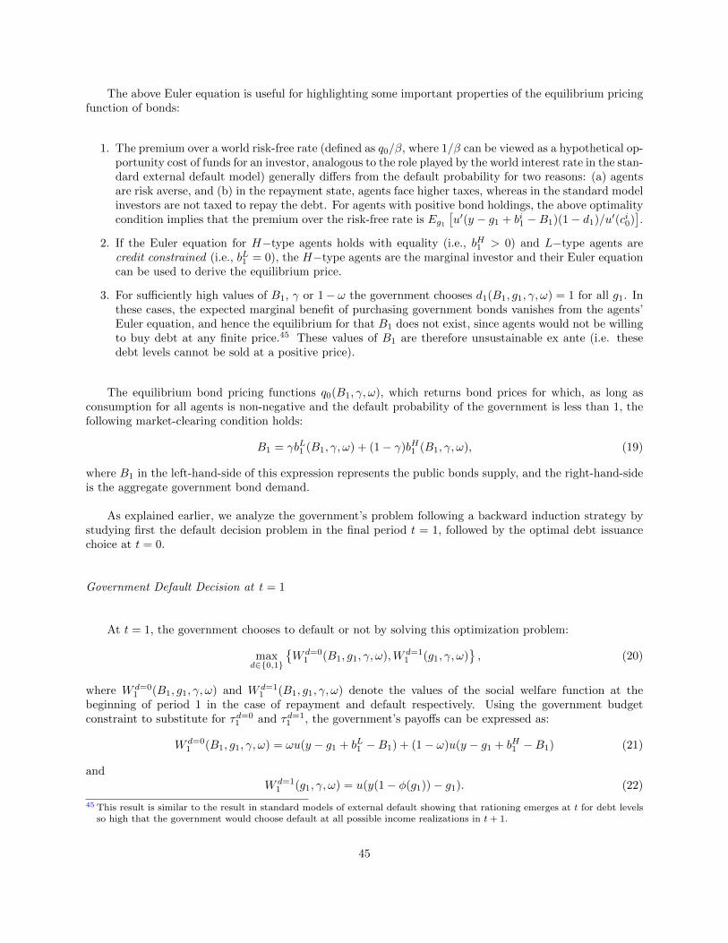
The above Euler equation is useful for highlighting some important properties of the equilibrium pricingfunction of bonds:

1. The premium over a world risk-free rate (defined as q0/β, where 1/β can be viewed as a hypothetical op-portunity cost of funds for an investor, analogous to the role played by the world interest rate in the stan-dard external default model) generally differs from the default probability for two reasons: (a) agentsare risk averse, and (b) in the repayment state, agents face higher taxes, whereas in the standard modelinvestors are not taxed to repay the debt. For agents with positive bond holdings, the above optimalitycondition implies that the premium over the risk-free rate is Eg1

[u′(y − g1 + bi1 −B1)(1− d1)/u′(ci0)

].

2. If the Euler equation for H−type agents holds with equality (i.e., bH1 > 0) and L−type agents arecredit constrained (i.e., bL1 = 0), the H−type agents are the marginal investor and their Euler equationcan be used to derive the equilibrium price.

3. For sufficiently high values of B1, γ or 1− ω the government chooses d1(B1, g1, γ, ω) = 1 for all g1. Inthese cases, the expected marginal benefit of purchasing government bonds vanishes from the agents’Euler equation, and hence the equilibrium for that B1 does not exist, since agents would not be willingto buy debt at any finite price.45 These values of B1 are therefore unsustainable ex ante (i.e. thesedebt levels cannot be sold at a positive price).

The equilibrium bond pricing functions q0(B1, γ, ω), which returns bond prices for which, as long asconsumption for all agents is non-negative and the default probability of the government is less than 1, thefollowing market-clearing condition holds:

B1 = γbL1 (B1, γ, ω) + (1− γ)bH1 (B1, γ, ω), (19)

where B1 in the left-hand-side of this expression represents the public bonds supply, and the right-hand-sideis the aggregate government bond demand.

As explained earlier, we analyze the government’s problem following a backward induction strategy bystudying first the default decision problem in the final period t = 1, followed by the optimal debt issuancechoice at t = 0.

Government Default Decision at t = 1

At t = 1, the government chooses to default or not by solving this optimization problem:

maxd∈{0,1}

{W d=0

1 (B1, g1, γ, ω),W d=11 (g1, γ, ω)

}, (20)

where W d=01 (B1, g1, γ, ω) and W d=1

1 (B1, g1, γ, ω) denote the values of the social welfare function at thebeginning of period 1 in the case of repayment and default respectively. Using the government budgetconstraint to substitute for τd=0

1 and τd=11 , the government’s payoffs can be expressed as:

W d=01 (B1, g1, γ, ω) = ωu(y − g1 + bL1 −B1) + (1− ω)u(y − g1 + bH1 −B1) (21)

andW d=1

1 (g1, γ, ω) = u(y(1− φ(g1))− g1). (22)

45 This result is similar to the result in standard models of external default showing that rationing emerges at t for debt levelsso high that the government would choose default at all possible income realizations in t+ 1.

45

Combining these payoff functions, if follows that the government defaults if this condition holds:

ω

u(y − g1 +

≤0︷ ︸︸ ︷(bL1 −B1))− u(y(1− φ(g1))− g1)

+ (23)

(1− ω)

u(y − g1 +

≥0︷ ︸︸ ︷(bH1 −B1))− u(y(1− φ(g1))− g1)

≤ 0

Notice that all agents forego g1 of their income to government absorption regardless of the default choice.Moreover, debt repayment reduces consumption and welfare of L types and rises them for H types, whereasdefault implies the same consumption and utility for both types of agents.

The distributional effects of a default are implicit in condition (23). Given that debt repayment affectsthe cash-in-hand for consumption of L and H types according to (bL1 −B1) ≤ 0 and (bH1 −B1) ≥ 0 respectively,it follows that, for a given B1, the payoff under repayment allocates (weakly) lower welfare to L agents andhigher to H agents, and that the gap between the two is larger the larger is B1. Moreover, since the defaultpayoffs are the same for both types of agents, this is also true of the difference in welfare under repayment v.default: It is higher for H agents than for L agents and it gets larger as B1 rises. To induce default, however,it is necessary not only that L agents have a smaller difference in the payoffs of repayment v. default, butthat the difference is negative (i.e. they must attain lower welfare under repayment than under default),which requires B1 > bL1 + yφ(g1). This also implies that taxes under repayment need to be necessarily largerthan under default, since τd=0

1 − τd=11 = B1.

We can illustrate the distributional mechanism driving the default decision by comparing the utilitylevels associated with the consumption allocations of the default and repayment states with those thatwould be socially efficient. To this end, it is helpful to express the values of hypothetical optimal privatedebt holdings in period 1 as bL1 = B1− ε and bH1 (γ) = B1 + γ

1−γ ε, for some ε ∈ [0, B1]. That is, ε represents a

given hypothetical decentralized allocation of debt holdings across agents.46 Consumption allocations underrepayment would therefore be cL1 (ε) = y − g1 − ε and cH1 (γ, ε) = y − g1 + γ

1−γ ε, so ε also determines thedecentralized consumption dispersion.

The government payoff under repayment can be rewritten as:

W d=0(ε, g1, γ, ω) = ωu(y − g1 + ε) + (1− ω)u

(y − g1 +

γ

1− γ ε).

The efficient dispersion of consumption that the social planner would choose is characterized by thevalue of εSP that maximizes social welfare under repayment. In the particular case of ω = γ (i.e., whenthe government is utilitarian and uses welfare weights that match the wealth distribution), εSP satisfies thisfirst-order condition:

u′(y − g1 +

γ

1− γ εSP

)= u′

(y − g1 − εSP

). (24)

Hence, the efficient allocations are characterized by zero consumption dispersion, because equal marginalutilities imply cL,SP=cH,SP = y − g1, which is attained with εSP = 0.

Continuing under the utilitarian government assumption (ω = γ), consider now the government’s defaultdecision when default is costless (φ(g1) = 0). Given that the only policy instruments the government can

46 We take ε as given at this point because it helps us explain the intuition behind the distributional default incentives of thegovernment, but ε is an equilibrium outcome solved for later on. Also, ε must be non-negative, otherwise H types would bethe non-bondholders.

46

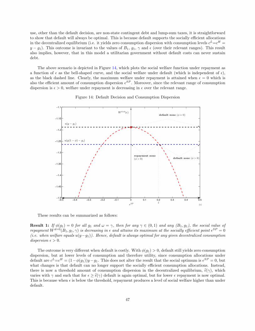
use, other than the default decision, are non-state contingent debt and lump-sum taxes, it is straightforwardto show that default will always be optimal. This is because default supports the socially efficient allocationsin the decentralized equilibrium (i.e. it yields zero consumption dispersion with consumption levels cL=cH =y − g1). This outcome is invariant to the values of B1, g1, γ and ε (over their relevant ranges). This resultalso implies, however, that in this model a utilitarian government without default costs can never sustaindebt.

The above scenario is depicted in Figure 14, which plots the social welfare function under repayment asa function of ε as the bell-shaped curve, and the social welfare under default (which is independent of ε),as the black dashed line. Clearly, the maximum welfare under repayment is attained when ε = 0 which isalso the efficient amount of consumption dispersion εSP . Moreover, since the relevant range of consumptiondispersion is ε > 0, welfare under repayment is decreasing in ε over the relevant range.

Figure 14: Default Decision and Consumption Dispersion

−0.5 −0.4 −0.3 −0.2 −0.1 0 0.1 0.2 0.3 0.4 0.5−1.5

−1.45

−1.4

−1.35

−1.3

−1.25

−1.2

−1.15

−1.1

(ǫ)

W d=0(ǫ)

ǫSP

u(y − g1)

u(y(1− φ)− g1)

ǫ

default zone (φ> 0)

default zone (φ= 0)

repayment zone

(φ> 0)

These results can be summarized as follows:

Result 1: If φ(g1) = 0 for all g1 and ω = γ, then for any γ ∈ (0, 1) and any (B1, g1), the social value ofrepayment W d=0(B1, g1, γ) is decreasing in ε and attains its maximum at the socially efficient point εSP = 0(i.e. when welfare equals u(y−g1)). Hence, default is always optimal for any given decentralized consumptiondispersion ε > 0.

The outcome is very different when default is costly. With φ(g1) > 0, default still yields zero consumptiondispersion, but at lower levels of consumption and therefore utility, since consumption allocations underdefault are cL=cH = (1−φ(g1))y−g1. This does not alter the result that the social optimum is εSP = 0, butwhat changes is that default can no longer support the socially efficient consumption allocations. Instead,there is now a threshold amount of consumption dispersion in the decentralized equilibrium, ε(γ), whichvaries with γ and such that for ε ≥ ε(γ) default is again optimal, but for lower ε repayment is now optimal.This is because when ε is below the threshold, repayment produces a level of social welfare higher than underdefault.

47

Figure 14 also illustrates this scenario. The default cost lowers the common level of utility of both typesof agents, and hence of social welfare, in the default state (shown in the Figure as the blue dashed line), andε(γ) is determined where social welfare under repayment and under default intersect. If the decentralizedconsumption dispersion with the debt market functioning (ε) is between 0 and less than ε(γ) then it is optimalfor the government to repay. Intuitively, if consumption dispersion is not too large, the government prefersto repay because the income cost imposed on agents to remove consumption dispersion under default is toolarge. Moreover, as γ rises the domain of W d=0

1 narrows, and thus ε(γ) falls and the interval of decentralizedconsumption dispersions that supports repayment narrows. This is natural because a higher γ causes theplanner to weight more L-types in the social welfare function, which are agents with weakly lower utility inthe repayment state.

These results can be summarized as follows:

Result 2: If φ(g1) > 0, then for any γ ∈ (0, 1) and any (B1, g1), there is a threshold value of consumptiondispersion ε(γ) such that the payoffs of repayment and default are equal: W d=0(B1, g1, γ) = u(y(1−φ(g1))−g1). The government repays if ε < ε(γ) and defaults otherwise. Moreover, ε(γ) is decreasing in γ.

Introducing a bias in the welfare function of the government (relative to utilitarian social welfare) canresult in repayment being optimal even without default costs, which provides for an alternative way tosustain debt subject to default risk. Assuming φ(g1) = 0, there are two possible scenarios depending onthe relative size of γ and ω. First, if ω > γ, the planner again always chooses default as in the setup withω = γ. This is because for any ε > 0, the decentralized consumption allocations feature cH > cL, while theplanner’s optimal consumption dispersion requires cH ≤ cL, and hence εSP cannot be implemented. Defaultbrings the planner the closest it can get to the payoff associated with εSP and hence it is always chosen.

In the second scenario ω < γ, which means that the government’s bias assigns more (less) weight to H(L) types than the fraction of each type of agents that actually exists. In this case, the model can supportequilibria with debt even without default costs. In particular, there is a threshold consumption dispersionε such that default is optimal for ε ≥ ε, where ε is the value of ε at which W d=0

1 (ε, g1, γ, ω) and W d=11 (g1)

intersect. For ε < ε, repayment is preferable because W d=01 (ε, g1, γ, ω) > W d=0

1 (g1). Thus, without defaultcosts, equilibria for which repayment is optimal require two conditions: (a) that the government’s bias favorsbond holders (ω < γ), and (b) that the debt holdings chosen by private agents do not produce consumptiondispersion in excess of ε.

Figure 15 illustrates the outcomes just described. This Figure plots W d=01 (ε, g1, γ, ω) for ω R γ. The

planner’s default payoff and the values of εSP for ω R γ are also identified in the plot. The vertical intercept of

W d=01 (ε, g1, γ, ω) is always W d=1(g1) for any values of ω and γ, because when ε = 0 there is zero consumption

dispersion and that is also the outcome under default. In addition, the bell-shaped form of W d=01 (ε, g1, γ, ω)

follows from u′(.) > 0, u′′(.) < 0.47

Take first the case with ω > γ. In this case, the planner’s payoff under repayment is the dotted bellcurve. Here, εSP < 0, because the optimality condition implies that the planner’s optimal choice featurescL > cH . Since default is the only instrument available to the government, however, these consumptionallocations are not feasible, and by choosing default the government attains W d=1, which is the highestfeasible government payoff for any ε ≥ 0. In contrast, in the case with ω = γ, for which the planner’s payofffunction is the dashed bell curve, the planner chooses εSP = 0, and default attains exactly the same payoff,so default is chosen. In short, if ω ≥ γ, the government always defaults for any decentralized distribution ofdebt holdings represented by ε > 0, and thus equilibria with debt cannot be supported.

47 Note in particular that∂Wd=0

1 (ε,g1,γ,ω)

∂εR 0 ⇐⇒ u′(cH (ε))

u′(cL(ε))R (ω

γ)( 1−γ

1−ω ). Hence, the planner’s payoff is increasing (decreas-

ing) at values of ε that support sufficiently low (high) consumption dispersion so thatu′(cH (ε))

u′(cL(ε))is above (below) (ω

γ)( 1−γ

1−ω ).

48

Figure 15: Default Decision with Non-Utilitarian Planner (φ = 0)

0 (ǫ)

Wd=0(ǫ)

ǫSP (ω < γ) ǫ(ω < γ)ǫSP (ω = γ)ǫSP (ω > γ)

ω < γ

ω = γ

ω > γ

Wd=1

u(y− g)

Repayment Zone

Default

Zone

When ω < γ, the planner’s payoff is the continuous curve. The intersection of the downward-slopingsegment of W d=0

1 (ε, g1, γ, ω) with W d=1 determines the default threshold ε such that default is optimal onlyin the default zone where ε ≥ ε. Default is still a second-best policy for the planner, because with it theplanner cannot attain W d=0(εSP ), it just gets the closest it can get. In contrast, the choice of repayment ispreferable in the repayment zone where ε < ε,, because in this zone W d=0

1 (ε, g1, γ, ω) > W d=1(g1).

Adding default costs to this political bias setup (φ(g1) > 0) makes it possible to support repaymentequilibria even when ω ≥ γ. As Figure 16 shows, with default costs there are threshold values of consumptiondispersion, ε, separating repayment from default zones for ω Q γ.

It is also evident in Figure 16 that the range of values of ε for which repayment is chosen widens as γrises relative to ω. Thus, when default is costly, equilibria with repayment require only the condition thatthe debt holdings chosen by private agents, which are implicit in ε, do not produce consumption dispersionlarger than the value of ε associated with a given (ω,γ) pair. Intuitively, the consumption of H-type agentsmust not exceed that of L-type agents by more than what ε allows, because otherwise default is optimal.

The fact that a government biased in favor of bond holders can find it optimally to repay may seemunsurprising. As we argue later, however, in fact governments with this bias can be an endogenous outcomeof majority voting if the fraction of agents that are non-bondholders is sufficiently large. This occurs whenthese agents are liquidity constrained (i.e. hitting the no-borrowing constraint), because in this case theyprefer that the government favors bondholders so that it can sustain higher debt levels because public debtprovides them with liquidity.

Government Debt Issuance Decision at t = 0

49

Figure 16: Default Decision with Non-Utilitarian Planner when φ(g1) > 0

0ǫ

Wd=0(ǫ)

ǫ(ω < γ)ǫ(ω = γ)ǫ(ω > γ)

ω < γ

ω = γ

ω > γ

u(y(1 − φ)− g)

u(y− g)

Wd=1

Wd=1

We are now in a position to study how the government chooses the optimal amount of debt to issuein the initial period. These are the model’s predicted sutainable debt levels ex ante, some of which will beoptimally defaulted on ex post, depending on the realization of g1in the second period. Both the governmentand the private sector are aware of this, so the debt levels that can be issued at equilibrium in the firstperiod are traded at prices that can carry a default risk premium, which will be the case if for a given debtstock there are some values of g1 for which default is the optimal choice in the second period.

The government’s optimization problem is easier to understand if we first illustrate how public debtserves as a tool for altering consumption dispersion across agents both within a period and across periods.In particular, consumption dispersion in each period and repayment state is given by these conditions:

cH0 − cL0 =1

1− γ [B0 − q0(B1, γ, ω)B1]

cH,d=01 − cL,d=0

1 =1

1− γB1

cH,d=11 − cL,d=1

1 = 0.

These expressions make it clear that, given B0, issuing at least some debt (B1 > 0) reduces consumptiondispersion at t = 0 compared with no debt (B1 = 0), but increases it at t = 1 if the government repays(i.e., d = 0). Moreover, the use of debt as tool for redistribution of consumption at t = 0 is hampered by aLaffer curve relationship just like the distortionary taxes of the previous Section. In this case, it takes theform of the debt Laffer curve familiar from the external default literature, which is defined by the mappingfrom an amount of debt issued B1 to the resources the government acquires with that amount of borrowing,q0(B1, γ, ω)B1. This mapping behaves like a Laffer curve because higher debt issuance carries a higherdefault risk, which reduces the price of the debt. Near zero debt the default risk is also zero so higher debtincreases resources for the government, at very high debt near the region at which debt is unsustainable exante, higher debt reduces resources because the price falls proportionally much more than the debt rises,and in between we obtain the bell-shaped Laffer curve relationship. It follows then from this Laffer curve

50

that, starting from B1 = 0, consumption dispersion at t = 0 first falls as B1 increases, but there is a criticalpositive value of B1 beyond which it becomes an increasing function of debt.

At t = 0, the government chooses its debt policy internalizing the above consumption dispersion effects,including the debt Laffer curve affecting date-0 dispersion, and their implications for social welfare. Formally,the government chooses B1 so as to maximize the “indirect” social welfare function:

W0(γ, ω) = maxB1

{ωvL(B1, γ, ω) + (1− ω)vH(B1, γ, ω)

}. (25)

where vL and vH are the private agents’ value functions obtained from solving the problems defined in theBellman equation (17) taking into account the government budget constraints and the equilibrium pricingfunction of bonds.

Focusing on the case with utilitarian government (ω = γ), we can gain some intuition about the solu-tion of this maximization problem from its first-order condition (assuming that the relevant functions aredifferentiable):

u′(cH0 ) = u′(cL0 ) +η

q0(B1, γ, ω)γ

{βEg1 [∆d∆W1] + γµL

}where

η ≡ q0(B1, γ, ω)/ (q′0(B1, γ, ω)B1) < 0,

∆d ≡ d(B1 + δ, g1, γ)− d(B1, g1, γ) ≥ 0, for δ > 0 small,

∆W1 ≡ W d=11 (g1, γ)−W d=0

1 (B1, g1, γ) ≥ 0,

µL ≡ q0(B1, γ, ω)u′(cL0 )− βEg1[(1− d1)u′(cL1 )

]> 0.

In these expressions, η is the price elasticity of the demand for government bonds, ∆d∆W1 represents themarginal distributional benefit of a default, and µL is the shadow value of the borrowing constraint when itbinds for L-type agents.

If both types of agents could be unconstrained in their savings decisions, so that µL = 0, and ifthere is no change in the risk of default (or assuming commitment to remove default risk entirely), sothat Eg1 [∆d∆W1] = 0, then the optimality condition simplifies to:

u′(cH0 ) = u′(cL0 ).

Hence, in this case the social planner would want to issue debt so as to equalize marginal utilities of con-sumption across agents at date 0, which requires simply setting B1 to satisfy q0(B1, γ, ω)B1 = B0. If it is thecase that L-types are constrained (i.e. µL > 0), and still assuming no change in default risk or a governmentcommitted to repay, the optimality condition becomes:

u′(cH0 ) = u′(cL0 ) +ηµL

q0(B1, γ, ω).

Since η < 0, this result implies cL0 < cH0 , because u′(cL0 ) > u′(cH0 ). Thus, even with unchanged default riskor no default risk at all, the government’s debt choice sets B1 as needed to maintain an optimal, positivelevel of consumption dispersion, which is the one that supports an excess in marginal utility of L-type agents

relative to H-type agents equal to ηµL

q0(B1,γ,ω) . Moreover, since optimal consumption dispersion is positive,

we can also ascertain that B0 > q0(B1, γ, ω)B1, which using the government budget constraint implies thatthe government runs a primary surplus at t = 0. The government borrows resources, but less than it wouldneed in order to eliminate all consumption dispersion (which requires zero primary balance).

The intuition for the optimality of issuing debt can be presented in terms of tax smoothing and savings:Date-0 consumption dispersion without debt issuance would be B0/(1− γ), but this is more dispersion than

51

what the government finds optimal, because by choosing B1 > 0 the government provides tax smoothing(i.e. reduces date-0 taxes) for everyone, which in particular eases the L-type agents credit constraint,and provides also a desired vehicle of savings for H types. Thus, positive debt increases consumption ofL types (since cL0 = y − g0 − B0 + q0(B1, γ, ω)B1), and reduces consumption of H types (since cH0 =

y − g0 +(

γ1−γ

)(B0 − q0(B1, γ, ω)B1)). But issuing debt (assuming repayment) also increases consumption

dispersion a t = 1, since debt is then paid with higher taxes on all agents, while H agents collect alsothe debt repayment. Thus, the debt is being chosen optimally to trade off the social costs and benefits ofreducing (increasing) date-0 consumption and increasing (reducing) date-1 consumption for agents who arebondholders (non-bondholders). In doing so, the government internalizes the debt Laffer curve and the factthat additional debt lowers the price of bonds and helps reduce µL, which in turn reduces the government’soptimal consumption dispersion.48

In the presence of default risk and if default risk changes near the optimal debt choice, the termEg1 [∆d∆W1] enters in the government’s optimality condition with a positive sign, which means the op-timal gap in the date-0 marginal utilities across agents widens even more. Hence, the government’s optimalchoice of consumption dispersion for t = 0 is greater than without default risk, and the expected dispersionfor t = 1 is lower, because in some states of the world the government will choose to default and consumptiondispersion would then drop to zero. This also suggests that the government chooses a lower value of B1 thanin the absence of default risk, since date-0 consumptions are further apart. Moreover, the debt Laffer curvenow plays a central role in the government’s weakened incentives to borrow, because as default risk rises theprice of bonds drops to zero faster and the resources available to reduce date-0 consumption dispersion peakat lower debt levels. In short, default risk reduces the government’s ability to use non-state-contingent debtin order to reduce consumption dispersion.

In summary, the more constrained the L−types agents are (higher µL) or the higher the expecteddistributional benefit of a default (higher Eg1 [∆d∆W1]), the larger the level of debt the government findsoptimal to issue. Both of these mechanisms operate as pecuniary externalities: They matter only becausethe government debt choice can alter the equilibrium price of bonds which is taken as given by private agents.

For given values of γ and ω, a Competitive Equilibrium with Optimal Debt and Default Policies is a pairof value functions vi(B1, γ, ω) and decision rules bi(B1, γ, ω) for i = L,H, a government bond pricing func-

tion q0(B1, γ, ω) and a set of government policy functions τ0(B1, γ, ω), τd∈{0,1}1 (B1, g1, γ, ω), d(B1, g1, γ, ω),

B1(γ, ω) such that:

1. Given the pricing function and government policy functions, vi(B1, γ, ω) and bi1(B1, γ, ω) solve thehouseholds’ problem.

2. q0(B1, γ, ω) satisfies the market-clearing condition of the bond market (equation (19)).

3. The government default decision d(B1, g1, γ, ω) solves problem (20).

4. Taxes τ0(B1, γ, ω) and τd1 (B1, g1, γ, ω) are consistent with the government budget constraints.

5. The government debt policy B1(γ, ω) solves problem (25).

48 Note, however, that without default risk the Laffer curve has less curvature than with default risk, because qND0 (B1, γ) =q0(B1, γ).

52

4.3 Quantitative Analysis

We study the quantitative predictions of the model using a calibration based on European data. Since themodel is simple, the goal is not to match closely the observed dynamics of debt and risk premia in Europe,but to show that a reasonable set of parameter values can support an equilibrium in which sustainable debtsubject to default risk exists.49 We also use this numerical analysis to study show the dispersion of initialwealth and the bias in government welfare affect sustainable debt.

4.3.1 Calibration

The model is calibrated to annual frequency, and most of the parameter values are set to match momentscomputed using European data. The parameter values that need to be set are the subjective discountfactor β, the coefficient of relative risk aversion σ, the moments of the stochastic process of governmentexpenditures {µg, ρg, σg}, the initial levels of government debt and expenditures (B0, g0), the level of incomey, the initial wealth of L−type agents bL0 and the default cost function φ(g1). The calibrated parameter valuesare summarized in Table 13. We evaluate equilibrium outcomes for values of γ and ω in the [0, 1] interval.Data for the United States and Europe documented in D’Erasmo and Mendoza (2013) suggest that theempirically relevant range for γ is [0.55, 0.85]. Hence, when taking a stance on a particular value of γ isuseful we use γ = 0.7, which is the mid point of the plausible range.

The preference parameters are set to standard values: β = 0.96, σ = 1. We also assume for simplicitythat L−types start with zero wealth, bL0 = 0.50 This and the other calibration parameters result in savingsplans such that L-type agents are credit constrained, and hence bL1 = 0.

We estimate an AR(1) process for government expenditures-GDP ratio (in logs) for France, Germany,Greece, Ireland, Italy, Spain and Portugal and set {µg, ρg, σg} to the cross-country averages of the corre-sponding estimates. This results in the following values µg = 0.1812, ρg = 0.8802 and σe = 0.017. We setg0 = µg and use the quadrature method proposed by Tauchen (1986) with 45 nodes in G1 ≡ {g1

, . . . , g1} togenerate the realizations and transition probabilities of g1.

Average income y is calibrated such that the model’s aggregate resource constraint is consistent with thedata when GDP is normalized to one. This implies that the value of the agents’ aggregate endowment mustequal GDP net of fixed capital investment and net exports, since the latter two are not modeled. The averagefor the period 1970-2012 for the same set of countries used to estimate the g1 process implies y = 0.7883.51

We set the initial debt level B0 = 0.79 so that at the maximum observed level of inequality in the data,γ = 0.85, there is at least one feasible level of B1 when ω = γ. We assume that the default cost takes thefollowing form: φ(g1) = φ0 + (g − g1)/y, where g is calibrated to represent an “unusually large” realizationof g1 set equal to the largest realization in the Markov process of government expenditures, which is in turnset equal to 3 standard deviations from the mean (in logs).52

49 We solve the model following a backward-recursive strategy analogous to the one used in the theoretical analysis. First, foreach pair {γ, ω} and taking as given B1, we solve for the equilibrium price and default functions by iterating on {d1, q0, bi1}.Then, in the second stage we complete the solution of the equilibrium by finding the optimal choice of B1 that solves thegovernment’s date-0 optimization problem (25). As explained earlier, for given values of B1, γ and ω an equilibrium withdebt will not exist if either the government finds it optimal to default on B1 for all realizations of g1 or if at the given B1

the consumption of L types is non-positive.50 σ = 1 and bL0 = 0 are also useful because under these assumptions we can obtain closed-form solutions and establish some

results analytically.51 Note also that under this calibration of y and the Markov process of g1, the gap y − g1 is always positive, even for g1 = g1,

which in turn guarantees cH1 > 0 in all repayment states.52 This cost function shares a key feature of the default cost functions widely used in the external default literature to align

53

We calibrate φ0 to match an estimate of the observed frequency of domestic defaults. According toReinhart and Rogoff (2011), historically, domestic defaults are about 1/4 as frequent as external defaults(68 domestic v. 250 external in their data since 1750). Since the probability of an external default has beenestimated in the range of 3 to 5 percent (see, for example, Arellano (2008)), the probability of a domesticdefault is about 1 percent. The model is close to this default frequency on average when solved over theempirically relevant range of γ′s (γ ∈ [0.55, 0.85]) if we set φ0 = 0.02. Note, however, that the calibrationof φ0 and B0 to match their corresponding targets needs to be done jointly by repeatedly solving the modeluntil both targets are well approximated.

4.3.2 Utilitarian Government (ω = γ)

We study first a set of results obtained under the assumption ω = γ, because the utilitarian government is anatural benchmark. Since the default decision of the government derives from the agents’ utility under therepayment and default alternatives at t = 1, it is useful to map the ordinal utility measures into cardinalmeasures by computing “individual welfare gains of default,” which are standard consumption-equivalentvalues that equalize utility under default and repayment. Given the CRRA functional form, the individualwelfare gains of default reduce simply to the percent changes in consumption across the default and no-defaultstates of each agent at t = 1:

αi(B1, g1, γ) =ci,d=11 (B1, g1, γ)

ci,d=01 (B1, g1, γ)

− 1 =(1− φ(g1))y − g1

y − g1 + bi1 −B1− 1

A positive (negative) value of αi(B1, g1, γ) implies that agent i prefers government default (repayment) byan amount equivalent to an increase (cut) of αi(·) percent in consumption. The individual welfare gains ofdefault are aggregated using γ to obtain the utilitarian representation of the social welfare gain of default:

α(B1, g1, γ) = γαL(B1, g1, γ) + (1− γ)αH(B1, g1, γ).

A positive value indicates that default induces a social welfare gain and a negative value a loss.

Figure 17 shows two intensity plots of the social welfare gain of default for the ranges of values of B1 andγ in the vertical and horizontal axes respectively. Panel (i) is for a low value of government purchases, g

1,

set 3 standard deviations below µg, and panel (ii) is for a high value g1 set 3 standard deviations above µg .“No Equilibrium Zone”, represent values of (B1, γ) for which the debt market collapses and no equilibriumexists.53

The area in which the social welfare gains of default are well defined in these intensity plots illustratestwo of the key mechanisms driving the government’s distributional incentives to default: First, fixing γ, thewelfare gain of default is higher at higher levels of debt, or conversely the gain of repayment is lower. Second,keeping B1 constant, the welfare gain of default is also increasing in γ (i.e. higher wealth concentrationincreases the welfare gain of default). This implies that lower levels of wealth dispersion are sufficient totrigger default at higher levels of debt.54 For example, for a debt ratio of 20 percent of GDP (B1 = 0.20)

default incentives so as to support higher debt ratios and trigger default during recessions (see Arellano (2008) and Mendozaand Yue (2012)): The default cost is an increasing function of disposable income (y − g1). In addition, this formulationensures that the agents’ consumption during a default never goes above a given threshold.

53 Note that to determine if cL0 ≤ 0 at some (B1, γ) we also need q0(B1, γ), since combining the budget constraints of the L typesand the government yields cL0 = y − g0 −B0 + q0B1. Hence, to evaluate this condition we take the given B1 and use the H-types Euler equation and the market clearing condition to solve for q0(B1, γ, ω), and then determine if y−g0−B0+q0B1 ≤ 0,if this is true, then (B1, γ) is in the lower no- equilibrium zone.

54 Note that the cross-sectional variance of initial debt holdings is given by V ar(b) = B2 γ1−γ when bL0 = 0. This implies that

the cross-sectional coefficient of variation is equal to CV (b) = γ1−γ , which is increasing in γ for γ ≤ 1/2.

54

Figure 17: Social Welfare Gains of Default α(B1, g1, γ)

Note: The intensity of the color or shading in these plots indicates the magnitude of the welfare gain according to the legend

shown to the right of the plots. The regions shown in white and marked as “No Equilibrium Zone”, represent values of (B1, γ)

for which the debt market collapses and no equilibrium exists.

55

and g1 = g1, social welfare is higher under repayment if 0 ≤ γ ≤ 0.25 but it becomes higher under default if0.25 < γ ≤ 0.6, and for higher γ there is no equilibrium because the government prefers default not only forg1 = g1 but for all possible g1. If instead the debt is 40 percent of GDP, then social welfare is higher underdefault for all the values of γ for which an equilibrium exists.

The two panels in Figure 17 differ in that panel (ii) displays a well-defined transition from a region inwhich repayment is socially optimal (α(B1, g1, γ) < 0) to one where default is optimal (α(B1, g1, γ) > 0) butin panel (i) the social welfare gain of default is never positive, so repayment is always optimal. This reflectsthe fact that higher g1 also weakens the incentives to repay. In the “No Equilibrium Zone” in the upperright, there is no equilibrium because at the given γ the government chooses to default on the given B1 forall values of g1. In the “No Equilibrium Zone” in the lower left, there is no equilibrium because the given(B1, γ) would yield cL0 ≤ 0, and so the government would not supply that particular B1.

Consider next the government’s default decision choice, which is driven by the sign of the social welfaregains of default. It is evident from Figure 17 that the government defaults the higher g1 for given B1 and γ,the higher B1 for a given γ and g1, or at higher γ at given B1 and g1. It follows then that we can compute athreshold value of γ such that the government is indifferent between defaulting and repaying in period t = 1for a given (B1, g1). These indifference thresholds (γ(B1, g1)) are plotted in Figure 18 against debt levelsranging from 0 to 0.4 for three values of government expenditures {g1, µg, g1}. For any given (B1, g1), thegovernment chooses to default if γ ≥ γ.

Figure 18: Default Threshold γ(B1, g1)

0 0.05 0.1 0.15 0.2 0.25 0.3 0.35 0.40

0.1

0.2

0.3

0.4

0.5

0.6

0.7

0.8

0.9

1

Gov. Debt (B1)

Defau

ltThresho

ld(γ)

γ(B1, g)

γ(B1, µg)γ(B1, g)

Figure 18 shows that the default threshold is decreasing in B1. Hence, the government tolerates higherdebt ratios without defaulting only if wealth concentration is sufficiently low. Also, default thresholds aredecreasing in g1, because the government has stronger incentives to default when government expendituresare higher (i.e. the threshold curves shift inward).55 This last feature of γ is very important to determineequilibria with sustainable debt subject to default risk. If, for a given value of B1, γ is higher than thecurve representing γ for the lowest realization in the Markov process of g1 (which is also the value of g1),

55 γ approaches zero for B1 sufficiently large, but in Figure 18 B1 reaches 0.40 only for exposition purposes.

56

the government defaults for sure and, as explained earlier, there is no sustainable debt at equilibrium.Alternatively, if for a given value of B1, γ is lower than the curve representing γ for the highest realizationof g1 (which is the value of g1), the government repays for sure and debt would be issued effectively withoutdefault risk. Thus, for the model to support equilibria with sustainable debt subject to default risk, theoptimal debt chosen by the government in the first period for a given γ must lie between these two extremethreshold curves. We show below that this is the case in this quantitative experiment.

Before showing those results, it is important to highlight three key properties of the bond pricing function.The quantitative results for this function, the details of which we omit to save space, reflect the propertiesdiscussed in the model analysis:

1. The equilibrium price is decreasing in B1 for given γ (the pricing functions shift downward as B1 rises).This follows from a standard demand-and-supply argument: For a given γ, as the government borrowsmore, the price at which the H types are willing to demand the additional debt falls and the interestrate rises.

2. Default risk reduces the price of bonds below the risk-free price and thus induces a risk premium.Intuitively, when there is no default risk (i.e. for combinations of B1 and γ such that the probability ofdefault is zero) both prices are identical. However, as the probability of default rises, agents demanda premium in order to clear the bond market.

3. Bond prices are a non-monotonic function of wealth dispersion: When default risk is sufficiently low,bond prices are increasing in γ, but eventually they become a steep decreasing function of γ. Higher γimplies a more dispersed wealth distribution, so that H-type agents become a smaller fraction of thepopulation, and hence they must demand a larger amount of debt per capita in order to clear the bondmarket (i.e. bH1 increases with γ), which pushes bond prices up. While default risk is low this “demandcomposition effect” dominates and thus bond prices rise with γ, but as γ increases and default risk rises(since higher wealth dispersion strengthens default incentives), the growing risk premium becomes thedominating force (at about γ > 0.5) and produces bond prices that fall sharply as γ increases.

Finally we examine the numerical solutions of the model’s full equilibrium with optimal debt and defaultpolicies. The key element of the solution is the sustainable debt, which is also the government’s optimalchoice of debt issuance in the first period at the equilibrium price (i.e. the optimal B1 that solves problem(25)). We show this sustainable debt as an equilibrium manifold (i.e. as a plot of the sustainable debtobtained by solving the model’s equilibrium over a range of values of γ). Given this sustainable debt, wecan then use the functions that describe optimal debt demand plans of private agents in both periods, thegovernment’s default choice in period 1, bond prices, and default risk for any value of B1 to determine thecorresponding equilibrium manifold values of all of the model’s endogenous variables.

Figure 19 shows the four main components of the equilibrium manifolds: Panel (i) plots the manifoldof sustainable first-period debt issuance of the model with default risk, B∗1(γ), and also, for comparison, thedebt in the case when the government is committed to repay so that debt is risk free, BRF1 (γ). Panel (ii)shows equilibrium debt prices that correspond to the sustainable debt of the same two economies. Panel(iii) shows the default spread (the difference in the inverses of the bond prices). Panel (iv) shows theprobability of default. Since in principle the government that has the option to default can still choose adebt level for which it could prefer to repay in all realizations of g1, we identify with a square in Panel (i) theequilibria in which B∗1(γ) has a positive default probability. This is the case for all but the smallest value ofgamma considered (γ = 0.05), in which the government sets B∗1(γ) at 40 percent of GDP with zero defaultprobability.

Panel (i) shows that sustainable debt falls as γ increases in both the economy with default risk andthe economy with a government committed to repay. This occurs because in both cases the government

57

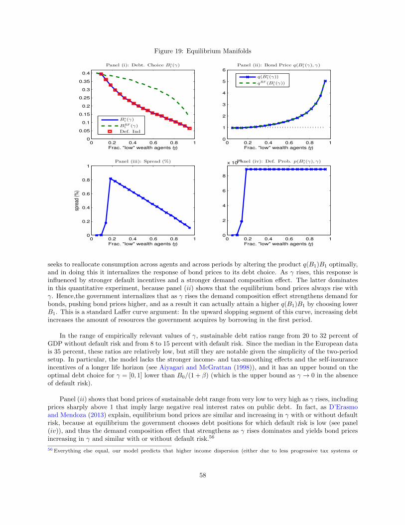
Figure 19: Equilibrium Manifolds

0 0.2 0.4 0.6 0.8 10

0.05

0.1

0.15

0.2

0.25

0.3

0.35

0.4

Frac. "low" wealth agents (γ)

Panel (i): Debt. Choice B∗

1(γ)

B∗

1(γ)

BRF1 (γ)

Def. Ind

0 0.2 0.4 0.6 0.8 10

1

2

3

4

5

6

Frac. "low" wealth agents (γ)

Panel (ii): Bond Price q(B∗

1(γ), γ)

q(B∗

1(γ))

qRF (B∗

1(γ))

0 0.2 0.4 0.6 0.8 10

0.2

0.4

0.6

0.8

1

Frac. "low" wealth agents (γ)

Panel (iii): Spread (%)

spre

ad (%

)

0 0.2 0.4 0.6 0.8 10

2

4

6

8

x 10−3

Frac. "low" wealth agents (γ)

Panel (iv): Def. Prob. p(B∗

1(γ), γ)

seeks to reallocate consumption across agents and across periods by altering the product q(B1)B1 optimally,and in doing this it internalizes the response of bond prices to its debt choice. As γ rises, this response isinfluenced by stronger default incentives and a stronger demand composition effect. The latter dominatesin this quantitative experiment, because panel (ii) shows that the equilibrium bond prices always rise withγ. Hence,the government internalizes that as γ rises the demand composition effect strengthens demand forbonds, pushing bond prices higher, and as a result it can actually attain a higher q(B1)B1 by choosing lowerB1. This is a standard Laffer curve argument: In the upward slopping segment of this curve, increasing debtincreases the amount of resources the government acquires by borrowing in the first period.

In the range of empirically relevant values of γ, sustainable debt ratios range from 20 to 32 percent ofGDP without default risk and from 8 to 15 percent with default risk. Since the median in the European datais 35 percent, these ratios are relatively low, but still they are notable given the simplicity of the two-periodsetup. In particular, the model lacks the stronger income- and tax-smoothing effects and the self-insuranceincentives of a longer life horizon (see Aiyagari and McGrattan (1998)), and it has an upper bound on theoptimal debt choice for γ = [0, 1] lower than B0/(1 + β) (which is the upper bound as γ → 0 in the absenceof default risk).

Panel (ii) shows that bond prices of sustainable debt range from very low to very high as γ rises, includingprices sharply above 1 that imply large negative real interest rates on public debt. In fact, as D’Erasmoand Mendoza (2013) explain, equilibrium bond prices are similar and increasing in γ with or without defaultrisk, because at equilibrium the government chooses debt positions for which default risk is low (see panel(iv)), and thus the demand composition effect that strengthens as γ rises dominates and yields bond pricesincreasing in γ and similar with or without default risk.56

56 Everything else equal, our model predicts that higher income dispersion (either due to less progressive tax systems or

58

Panels (iii) and (iv) show that, in contrast with standard models of external default, in this model thedefault spread is neither similar to the probability of default nor does it have a monotonic relationship withit.57 Both the spread and the default probability start at zero for γ = 0.05 because B∗1(0.05) has zero defaultprobability. As γ increases up to 0.2, both the spread and the default probability of the sustainable debtare similar in magnitude and increase together, but for γ > 0.2 the spread falls with γ while the defaultprobability remains unchanged around 0.9 percent. For γ = 0.95 the probability of default is 9 times largerthan the spread (0.9 v. 0.1 percent).

The role of the government’s incentives to reallocate consumption across agents and across periodsinternalizing the response of bond prices when choosing debt can be illustrated further by examining thedebt Laffer curve. Figure 20 shows debt Laffer curves for five values of γ in the [0.05,0.95] range.

Figure 20: Debt Laffer Curve

0 0.05 0.1 0.15 0.2 0.25 0.3 0.35 0.4

0.2

0.25

0.3

0.35

0.4

0.45

0.5”Laffer” Curve B1 ∗ q(B1, γ)

Government Debt (B1)

B1∗q(B

1,γ)

B1 ∗ q(B1, γ = 0.05)B1 ∗ q(B1, γ = 0.25)B1 ∗ q(B1, γ = 0.50)B1 ∗ q(B1, γ = 0.75)B1 ∗ q(B1, γ = 0.95)Bx

1

Note: Each curve is truncated at values of B1 in the horizontal axis that are either low enough for cL0 ≤ 0 or high enough for

default to be chosen for all realizations of g1, because as noted before in these cases there is no equilibrium.

In all but one case, the sustainable debt B∗1(γ) (i.e. the equilibrium debt chosen optimally by the gov-ernment at the equilibrium price) is located at the maximum of the corresponding Laffer curve. In thesecases, setting debt higher than at the maximum is suboptimal because default risk reduces bond pricessharply, moving the government to the downward-sloping segment of the Laffer curve. Setting debt lowerthan the maximum is also suboptimal, because then default risk is low and extra borrowing generates moreresources since bond prices change little, leaving the government in the upward-sloping segment region of

underlying households’ income or bond positions) results in higher spreads. In D’Erasmo and Mendoza (2013) we show thatan economy with more progressive tax system results in lower spreads. The intuition is simple. The more the governmentcan redistribute via means of taxation the lower the incentives to redistribute through a domestic default on the debt. Theresults in that paper show that incentives to default do not disappear but spreads decrease considerably. Also in D’Erasmoand Mendoza (2013), we present evidence of the non-linear relationship between debt to income ratios and wealth inequality.Data limitations prevents us from extending this analysis to the relationship between spreads and income dispersion or theprogressivity of the tax system.

57 In the standard models, the two are similar and a monotonic function of each other because of the arbitrage condition of arepresentative risk-neutral investor.

59

the Laffer curve. Thus, if the optimal debt has a nontrivial probability of default, the government’s debtchoice exhausts its ability to raise resources by borrowing. The exception is the case with γ = 0.05, in whichB∗1(γ) has zero default probability. In this case, the government’s optimal debt is to the left of the maximumof the Laffer curve, and thus the debt choice does not exhaust the government’s ability to raise resourcesby borrowing. This also happens when the default probability is positive but negligible. For example, whenγ = 0.15 the default probability is close to zero and the optimal debt choice is again slightly to the left ofthe maximum of the corresponding Laffer curve.

4.3.3 Biased Welfare Weights (ω 6= γ)

The final experiment we conduct examines how the results change if we allow the weights of the government’spayoff function to display a bias in favor of bondholders. Figure 21 shows how the planner’s welfare gain ofdefault varies with ω and γ for two different levels of government debt (B1,L = 0.143 and B1,H = 0.185).The no-equilibrium region, which exists for the same reasons as before, is shown in white.

Figure 21: Planner’s Welfare Gain of Default α(B1, g1, γ, ω)

In line with the previous discussion, within the region where the equilibrium is well-defined, the plan-ner’s value of default increases monotonically as ω increases, keeping γ constant, and falls as actual wealthconcentration (γ) rises, keeping ω constant. Because of this, the north-west and south-east corners in eachof the panels present cases that are at very different positions on the preference-for-default spectrum. Whenω is low, even for very high values of γ, the government prefers to repay (north-west corner), because the

60

government puts relatively small weight on L-type agents. On the contrary, when ω is high, even for lowlevels of γ, a default is preferred. It is also interesting to note that as we move from Panel (i) to Panel(ii), so that government debt raises, the set of γ’s and ω’s such that the equilibrium exists or repayment ispreferred (i.e. a negative α(B1, g1, γ, ω)) expands. This is because as we increase the level of debt B1, aslong as the government does not choose to default for all g1, the higher level of debt allows L-type agents toattain positive levels of consumption (since initial taxes are lower).

Panels (i)− (iv) in Figure 22 display the model’s equilibrium outcomes for the sustainable debt chosenby the government in the first period and the associated equilibrium bond prices, spreads and defaultprobabilities under three possible values of ω, all plotted as functions of γ. It is important to note that alongthe blue curve of the utilitarian case both ω and γ effectively vary together because they are always equalto each other, while in the other two plots ω is fixed and γ varies. For this reason, the line corresponding tothe ωL case intersects the benchmark solution when γ = 0.32, and the one for ωH intersects the benchmarkwhen γ = 0.50.

Figure 22: Equilibrium Manifolds with Government Bias at different values of ω

0 0.5 10

0.1

0.2

0.3

0.4

0.5

Frac. "low" wealth agents (γ)

Panel (i): Debt. Choice B∗

1(γ)

0 0.5 10

1

2

3

4

5

6

Frac. "low" wealth agents (γ)

Panel (ii): Bond Price q(B∗

1(γ), γ)

ω = γ (bench.)ωL

ωH

0 0.5 10

1

2

3

4

5

Frac. "low" wealth agents (γ)

Panel (iii): Spread (%)

spre

ad (

%)

0 0.5 10

0.01

0.02

0.03

0.04

0.05

0.06

Frac. "low" wealth agents (γ)

Panel (iv): Def. Prob. p(B∗

1(γ), γ)

Figure 22 shows that the optimal debt level is increasing in γ. This is because the incentives to defaultgrow weaker and the repayment zone widens as γ increases for a fixed value of ω. It is also interesting tonote that in the ωL and ωH cases the equilibrium exists only for a small range of values of γ that are lowerthan ω. Without default costs each curve would be truncated exactly where γ equals either ωH or ωH , butsince these simulations retain the default costs used in the utilitarian case, there can still be equilibria withdebt for some lower values of γ (as explained earlier).

With the bias in favor of bondholders, the government is still aiming to optimize debt by focusing on

61

the resources it can reallocate across periods and agents, which are still determined by the debt Laffer curveq0(.)B1, and internalizing the response of bond prices to debt choices.58 This relationship, however, behavesvery differently than in the benchmark model, because now higher sustainable debt is carried at increasingequilibrium bond prices, which leads the planner internalizing the price response to choose higher debt,whereas in the benchmark model lower debt was sustained at increasing equilibrium bond prices, which ledthe planner internalizing the price response to choose lower debt.59

The behavior of equilibrium bond prices (panel (ii)) with either ωL = 0.32 or ωH = 0.50 differs markedlyfrom the utilitarian case. In particular, the prices no longer display an increasing, convex shape, insteadthey are a relatively flat and non-monotonic function of γ. This occurs because the higher supply of bondsthat the government finds optimal to provide offsets the demand composition effect that increases individualdemand for bonds as γ rises.

The domestic default approach to study sustainable debt adds important insights to those obtained fromthe empirical and structural approaches, both of which assumed repayment commitment. In particular, panel(i) of Figure 19 shows that sustainable debt falls sharply once risk of default is present, even when it is verysmall, and that (if the government is utilitarian) sustainable debt falls sharply with the concentration of bondownership, because of the strengthened incentive to use default as a tool for redistribution. Hence, estimatesof sustainable debt based on models in which the government is assumed to be committed to repay are likelyto be too optimistic. Intuitively, one can infer that in the structural model, a given increase in the initial debtwould be harder to offset with higher primary balances if the interest rate at which those primary balances arediscounted rises with higher debt because of default risk. Moreover, the representative-agent assumption isalso likely to lead to optimistic estimates of sustainable debt, because representative-agents models abstractfrom the strong incentives to use debt default as a tool for redistribution across heterogeneous agents. Theseincentives are likely to be weaker than in the model in practice, because tax and transfer policies that wedid not include in the model can be used for redistribution as well. But when these other instruments havebeen exhausted, and if inequality in bond holdings is sufficiently concentrated, the incentives to default asvehicle for redistribution are likely to be very strong.

A second important insight from this analysis is that sustainable debt is higher if the government’spayoff function is biased in favor of bondholders, and can even exceed debt that is sustainable withoutdefault risk when the government has a utilitarian social welfare function. Furthermore, D’Erasmo andMendoza (2013) show that non-bondholders may prefer equilibria where the government favors bondholders,instead of being utilitarian, because higher sustainable debt help relax their liquidity constraints. Hence, atsufficiently high levels of concentration of bond ownership, a biased government can sustain high debt andthe biased government can be elected as a majority government.

The main caveat of this analysis is that, because it was based on a two-period model, it misses importantendogenous costs of default that would be added to the model by introducing a longer life horizon. In thiscase, default costs due to the reduced ability to smooth taxation and consumption when the debt marketcloses, and due to the loss of access to the self-insurance vehicle and the associated tightening of liquidityconstraints, can take up the role of the exogenous default costs and/or government bias for bondholders,enabling the model to improve its ability to account for key features of the data and sustain higher debtlevels at nontrivial default premia. D’Erasmo and Mendoza (2014) examine a model with these features andstudy its quantitative implications.

58 When choosing B1, the government takes into account that higher debt increases disposable income for L-type agents in theinitial period but it also implies higher taxes in the second period (as long as default is not optimal). Thus, the governmentis willing to take on more debt when ω is lower.

59 Figure 22 makes clear that with the government bias, the level of sustainable debt changes with the preferences of thegovernment. Even though we do not model how these preferences arise, it is evident that two countries with the samefundamentals (i.e. distribution of wealth and income) could end up with very different levels of sustainable debt dependingon how household preferences are aggregated by the government in power.

62

5 Critical Assessment and Outlook

We started this Chapter by noting that the question of what is a sustainable public debt has always beenparamount in the macroeconomics of fiscal policy. The question will remain paramount for years to come, asthe precarious public debt and deficit positions of many advanced and emerging economies today will makeit a central focus of both policy analysis and academic research. This Chapter aimed to demonstrate theflaws that affect the classic, but still widely used, approach to analyze public debt sustainability, and to showhow three approaches based on recent research can provide powerful alternative ways to tackle the question.Two of these approaches, the empirical approach and the structural approach, assume that the governmentis committed to repay its debt, and the third approach, the domestic default approach, assumes that thegovernment cannot commit to repay. In this Section of the Chapter we reflect further on the limitations ofeach of these approaches and suggest directions for further research.

The empirical approach has been widely studied and is by now very well established. Its strengths arein that it can easily determine whether debt has been consistent with fiscal solvency in available time-seriesdata via straightforward estimation of a fiscal reaction function, and in that analyzing the characteristics ofthis FRF it can shed light on the dynamics of adjustment of debt and the primary balance. Unfortunately,as we explained earlier, it is not helpful for comparing alternative fiscal policy strategies to maintain debtsustainability and/or cope with public debt crises in the future.

The structural approach showed how an explicit dynamic general equilibrium model can be used tocompare alternative fiscal policy strategies aimed at maintaining fiscals solvency at different levels of observedoutstanding debt. We used a variation of the workhorse two-country Neoclassical framework with exogenous,balanced growth in which endogenous capacity utilization and a limited tax allowance for capital depreciationallow the model to match a key feature of the data for fiscal sustainability analysis: The observed elasticityof the capital tax revenue. Yet, the model is also very limited inasmuch as it abstracts from other importantfeatures of the data. In particular, the model is purely “real”, and hence abstracts from the fact thatpublic debt is largely nominal debt denominated in domestic currencies, and also abstracts from linkagesbetween potentially important nominal rigidities, relative prices, and the evolution of government revenuesand outlays.

The model used in the structural approach also has the drawbacks that it abstracts from heterogene-ity in households and firms and assumes that agents are infinitely-lived. Hence, while it takes into ac-count important efficiency effects resulting from alternative fiscal policies, it cannot capture their distri-butional implications across agents and/or generations. The fiscal policy research on heterogeneous-agentsand overlapping-generations models has shown that these distributional effects can be quite significant, andhence it is important to develop models of debt sustainability that incorporate them. For instance, Aiyagari(1995) showed that reductions in capital taxes have adverse distributional consequences that can offset theefficiency gains emphasized in representative agent models. Aiyagari and McGrattan (1998) showed thatpublic debt has social value because it acts as vehicle to provide liquidity (i.e. relax borrowing constraints)of the agents at the low end of the wealth distribution, and Birkeland and Prescott (2006) provide a setupin which using debt to save for retirement dominates a tax-and-transfer system. Imrohoroglu, Kirao, andYamada (2016) and Braun and Joines (2015) also show how sophisticated overlapping-generations modelscan be applied to study debt-sustainability issues, with a particular focus on the implications of the adversedemographics dynamics facing Japan.

Of the approaches to debt sustainability analysis reviewed here, the domestic default approach is the onethat has been studied the least. We provided a very simple canonical model in which default on domesticdebt can emerge as an optimal outcome for a government with incentives to redistribute across debt holdersand non-holders, but clearly significant further research in this area is needed (in addition to the recent workby D’Erasmo and Mendoza (2014) and Dovis, Golosov, and Shourideh (2014) that we cited).

63

There are also two other directions in which research on debt sustainability should go. First, to model therole of public debt in financial intermediation in general and in financial stabilization policies in particular.In terms of the former, domestic banking systems are often large holders of domestic public debt, so adomestic default of the kind the third approach we examined seeks to explain tends to materialize in termsof a redistribution that hurts the balance sheets of banks. A deeper question in a similar vein is why publicdebt is such a high-demand asset, or liquidity vehicle, in modern financial systems. Macro/finance researchis looking into this questions, but introducing these considerations into debt sustainability analysis is stilla pending task. Regarding crisis-management policies, the aftermath of the global financial crisis has beencharacterized by strong demand for public debt instruments driven by quantitative easing policies and bythe new regulatory environment. This may account for the apparent paradox between the pessimistic fiscalprospects that the analysis of this Chapter presents and the observation that we currently observe near-zero and even negative yields on the public debt of some advanced economies (i.e. demand for public debtremains very strong despite the highly questionable capacity of governments to repay it through standardimprovements of the primary fiscal balance). But to be certain we need a richer model of debt sustainabilitythat incorporates both the long-term forces that drive the government’s capacity to repay and short-termdebt dynamics around a financial crisis in which demand for risk-free asset surges.

The second direction in which debt sustainability analysis needs to branch out is to develop tools toincorporate considerations of potential multiplicity of equilibria in public debt markets. The seminal workof Calvo (1988) showed how debt can move between two equilibria supported by self-fulfilling expectations.In one the debt is repaid because agents expect that the government will be able to access the debt market,and thus maintain the efficiency losses of taxation small enough to indeed generate enough revenue torepay. In the other, the government defaults because agents expect that it will not be able to access thedebt market and will be forced into highly distorting levels of taxation that indeed result in revenues thatare insufficient to repay. The external default literature has explored models with this kind of equilibriummultiplicity extensively, as documented in the corresponding Chapter of this handbook, and theoretical workapplying these ideas to domestic debt crises is also available, but research to incorporate this mechanisminto quantitative models of domestic debt sustainability is still needed.

6 Conclusions

What is a sustainable public debt? Assuming that the government is committed to repay, the answer is adebt that satisfies the intertemporal government budget constraint (i.e. a debt that is equal to the presentdiscounted value of the primary fiscal balance). In this Chapter we showed that the traditional approachto debt sustainability analysis is flawed. This approach uses the steady-state government budget constraintto define sustainable debt as the annuity value of the primary balance, but it cannot establish if current orprojected debt and primary balance dynamics are consistent with that debt level. We then discussed twoapproaches to study public debt sustainability under committment to repay: First, an empirical approach,based on a linear fiscal reaction function, according to which a positive, conditional response of the primarybalance to debt is sufficient to establish debt sustainability. Second, a structural approach based on a two-country variant of the workhorse Neoclassical dynamic general equilibrium model with an explicit fiscalsector. The model differs from the standard Neoclassical setup in that it introduces endogenous capacityutilization and a limited tax allowance for depreciation expenses in order to match the observed elasticity ofthe capital tax base to changes in capital taxes. In this setup, the initial debt that is sustainable is the onedetermined by the present value of primary balances evaluated using equilibrium allocations and prices.

Applications of these first two approaches to cross-country data produced key insights. With the empir-ical approach, we found in tests based on historical U.S. data and cross-country panels that the sufficiencycodition for public debt to be sustainable (the positive, conditional response of the primary balance to debt),

64

cannot be rejected. We also found, however, clear evidence showing that the fiscal dynamics observed in theaftemath of the recent surge in debt in advanced economies represent a significant structural break in theestimated reaction functions. Primary deficits have been too large, and are projected to remain too large,relative to what the fiscal reaction functions predict, and they are also large compared with those observedin the aftermath previous episodes of large surges in debt.

The structural approach differs from the empirical approach in that it can be used to evaluate thepositive and normative effects of alternative paths of fiscal adjustment to attain debt sustainability, whereasthe empirical approach is silent about these effects. We calibrated the model to U.S. and European dataand used it to quantify the effects of unilateral changes in capital and labor taxes, particularly their effectson sustainable debt. The results suggest key differences across Europe and the United States. For theUnited States, the results suggest that changes in capital taxes cannot make the observed increase in debtsustainable, while small increases in labor taxes could. For Europe, the model predicts that the capacityto use taxes to make higher debt ratios sustainable is nearly fully exhausted. Capital taxation is highlyinefficient (in the decreasing segment of dynamic Laffer curves), so cuts in capital taxes would be neededto restore fiscal solvency. Labor taxes are near the peak of the dynamic Laffer curve, and even if increasedto the maximum point they do not generate enough revenue to make the present value of the primarybalance match the observed surge in debt. In addition, international externalities of capital income taxeswere quantitatively large, which suggest that incentives for strategic interaction are non-trivial and couldlead to a classic race-to-the-bottom in capital income taxation.

The results of the applications of the empirical and structural approaches paint a bleak picture of theprospects for fiscal adjustment in advanced economies to restore fiscal solvency and make the post-2008 surgein public debt ratios sustainable. In light of these findings, and with the ongoing turbulence in Europeansovereign debt markets and recurrent debt ceiling debates in the United States, we examined a third approachto debt sustainability that relaxes the assumption of a government committed to repay and allows for therisk of default on domestic public debt. In this environmnet, debt is sustainable when it is part of theequilibrium that includes the optimal debt issuance and default choices of the government. The governmenthas incentives to default as a vehicle for redistribution across agents who are heterogeneous in wealth. Publicdebt is not sustainable in the absence of default costs or a political bias to weigh the welfare of bond holdersby more than their share of the wealth distribution. This is the case because without these assumptionsdefault is always the optimal choice that maximizes the social welfare function of a government who valuesthe utility of all agents, and this is the case regardless of the present value of primary balances used tocharacterize sustainable debt under the other two approaches.

Quantitatively, this domestic default approach adds valuable insights to those obtained from the empiricaland structural approaches without default risk. In particular, sustainable debt falls sharply once risk ofdefault is present, even when it is very small, and it also falls sharply with wealth inequality, because of thestrengthened incentive to use default as a tool for redistribution. Hence, estimates of sustainable debt basedon models in which the government is assumed to be committed to repay are too optimistic. Moreover, therepresentative-agent assumption is also likely to lead to optimistic estimates of sustainable debt, becausemodels in this class abstract from the strong incentives to use debt default as a tool for redistribution acrossheterogeneous agents. A second important insight from the domestic default approach is that sustainabledebt is higher if the government’s payoff function weighs the welfare of bond hoders more heavily than theirshare of the wealth distribution. In addition, it is possible that low-wealth agents may also prefer that thegovernment weights high-wealth agents more heavily, instead of acting as a utilitarian government, becausehigher debt stocks help relax their liquidity constraints.

The three approaches reviewed in this Chapter provide useful tools for conducting debt sustainabilityanalysis. When applied to the current fiscal situation of advanced economies, all three suggest that substan-tial fiscal adjustment is still needed, is likely to entail substantial welfare costs, and is likely to continue to

65

be challenged by potential default risk in domestic sovereign debt markets.

66

References

Afonso, Antonio, 2005. “Fiscal Sustainability: The Unpleasant European Case.” FinanzArchiv: Public Fi-nance Analysis, 61(1): 19–, URL http://ideas.repec.org/a/mhr/finarc/urnsici0015-2218(200503)

611_19fstuec_2.0.tx_2-r.html.

Aghion, P. and P. Bolton, 1990. “Government Domestic Debt and the Risk of Default: A Political-Economic Model of the Strategic Role of Debt.” In Public Debt Management: Theory and History, editedby Rudiger Dornbusch and Mario Draghi. New York: Cambridge University Press: 315–44.

Aguiar, M. and M. Amador, 2013. “Fiscal Policy in Debt Constrained Economies.” NBER WorkingPapers 17457.

Aguiar, M., M. Amador, E. Farhi, and G. Gopinath, 2013. “Crisis and Commitment: InflationCredibility and the Vulnerability to Sovereign Debt Crises.” NBER Working Papers 19516.

Aiyagari, R. and E. McGrattan, 1998. “The optimum quantity of debt.” Journal of Monetary Economics,42: 447–469.

Aiyagari, R., A. Marcet, T. Sargent, and J. Seppala, 2002. “Optimal Taxation without State-Contingent Debt.” Journal of Political Economy, 110(6): 1220–1254.

Aiyagari, S. Rao, 1995. “Optimal Capital Income Taxation with Incomplete Markets, Borrowing Con-straints, and Constant Discounting.” Journal of Political Economy, 103(6): 1158–1175.

Alesina, A. and G. Tabellini, 1990. “A Positive Theory of Fiscal Deficits and Government Debt.” TheReview of Economic Studies, 57: 403–414.

Alesina, Alberto and Guido Tabellini, 2005. “Why is Fiscal Policy Often Procyclical?” Working Paper11600, National Bureau of Economic Research, URL http://www.nber.org/papers/w11600.

Amador, M., 2003. “A Political Economy Model of Sovereign Debt Repayment.” Stanford Universitymimeo.

Andreasen, E., G. Sandleris, and A. Van der Ghote, 2011. “The Political Economy of SovereignDefaults.” Universidad Torcuato Di Tella, Business School Working Paper.

Arellano, C., 2008. “Default Risk and Income Fluctuations in Emerging Economies.” American EconomicReview, 98(3): 690–712.

Auray, Stephane, Aurelien Eyquem, and Paul Gomme, 2013. “A Tale of Tax Policies in OpenEconomies.” mimeo, Department of Economics, Concordia University.

Azzimonti, M., E. de Francisco, and V. Quadrini, 2014. “Financial Globalization, Inequality, and theRising Public Debt.” American Economic Review, 104(8): 2267–2302.

Barnhill, Jr., M. Theodore, and G. Kopits, 2003. “Assessing Fiscal Sustainability Under Uncertainty.”IMF Working Paper, WP 03-79.

Barro, R., 1979. “On the determination of the public debt.” Journal of Political Economy, 87(5): 940–971.

Basu, S., 2009. “Sovereign debt and domestic economic fragility.” Manuscript, Massachusetts Institute ofTechnology.

Birkeland, K. and E. C. Prescott, 2006. “On the Needed Quantity of Government Debt.” ResearchDepartment, Federal Reserve Bank of Minneapolis, Working Paper 648.

67

Blanchard, Oliver J., Jean-Claude Chouraqui, Robert P. Hagemann, and Nichola Sartor, 1990.“The Sustainability of Fiscal Policy: New Answers to an Old Question.” OECD Economic Studies, 15(2):7–36.

Blanchard, Olivier J., 1990. “Suggestions for a New Set of Fiscal Indicators.” OECD Economics De-partment Working Papers 79, OECD Publishing, URL http://ideas.repec.org/p/oec/ecoaaa/79-en.

html.

Bocola, L., 2014. “The Pass-Through of Sovereign Risk.” Manuscript, University of Pennsylvania.

Bohn, H., 2011. “The Economic Consequences of Rising U.S. Government Debt: Privileges at Risk.”Finanzarchiv: Public Finance Analysis, 67 (3): 282–302.

Bohn, Henning, 1995. “The Sustainability of Budget Deficits in a Stochastic Economy.” Jour-nal of Money, Credit and Banking, 27(1): 257–71, URL http://ideas.repec.org/a/mcb/jmoncb/

v27y1995i1p257-71.html.

Bohn, Henning, 1998. “The Behavior Of U.S. Public Debt And Deficits.” The Quarterly Journal of Eco-nomics, 113(3): 949–963, URL http://ideas.repec.org/a/tpr/qjecon/v113y1998i3p949-963.html.

Bohn, Henning, 2007. “Are stationarity and cointegration restrictions really necessary for the intertemporalbudget constraint?” Journal of Monetary Economics, 54(7): 1837–1847, URL http://ideas.repec.org/

a/eee/moneco/v54y2007i7p1837-1847.html.

Bohn, Henning, 2008. “The Sustainability of Fiscal Policy in the United States.” In Reinhard Neck andJan-Egbert Sturm, eds., “Sustainability of public debt,” Cambridge, Mass.: MIT Press.

Boz, E., P. D’Erasmo, and B. Durdu, 2014. “Sovereign Risk and Bank Balance Sheets: The Role ofMacroprudential Policies.” Manuscript.

Braun, R.A. and D.H. Joines, 2015. “The implications of a graying Japan for government policy.”Journal of Economic Dynamics and Control, 57: 1 – 23.

Broner, F. and J. Ventura, 2011. “Globalization and Risk Sharing.” Review of Economic Studies, 78(1):49–82.

Broner, F., A. Martin, and J. Ventura, 2010. “Sovereign Risk and Secondary Markets.” AmericanEconomic Review, 100(4): 1523–55.

Brutti, 2011. “Sovereign defaults and liquidity crises.” Journal of International Economics, 84 (1): 65–72.

Buiter, Willem H, 1985. “A guide to public sector debt and deficits.” Economic policy, 1(1): 13–61.

Calvo, G., 1988. “Servicing the Public Debt: The Role of Expectations.” American Economic Review,78(4): 647–61.

Carey, David and Harry Tchilinguirian, 2000. “Average Effective Tax Rates on Capital, Labour andConsumption.” OECD Economics Department Working Papers: 258.

Chalk, Nigel Andrew and Richard Hemming, 2000. Assessing fiscal sustainability in theory and prac-tice. International Monetary Fund.

Chari, V. V., Lawrence J. Christiano, and Patrick J. Kehoe, 1994. “Optimal Fiscal Policy in aBusiness Cycle Model.” Journal of Political Economy, 102(4): 617–652.

Cooley, Thomas F and Gary D Hansen, 1992. “Tax distortions in a neoclassical monetary econ-omy.” Journal of Economic Theory, 58(2): 290 – 316, URL http://www.sciencedirect.com/science/

article/pii/002205319290056N.

68

Cuadra, G., Sanchez J., and Sapriza H., 2010. “Fiscal Policy and Default Risk in Emerging Markets.”Review of Economic Dynamics, 13(2): 452–469.

Davies, J., S. Sandstr02m S., A. Shorrocks, and E. Wolff, 2009. “The Level and Distribution ofGlobal Household Wealth.” NBER Working Paper 15508.

D’Erasmo, P., 2011. “Government Reputation and Debt Repayment in Emerging Economies.” mimeo.

D’Erasmo, P. and E. Mendoza, 2013. “Distributional incentives in an equilibrium model of domesticsovereign default.” National Bureau of Economic Research, No. w19477.

D’Erasmo, P. and E. Mendoza, 2014. “Optimal Domestic Sovereign Default.” Manuscript, University ofPennsylvania.

Di Casola, P. and S. Sichlimiris, 2014. “Domestic and External Sovereign Debt.” Working Paper, Stock-holm School of Economics.

Dias, D., C. Richmond, and M. Wright, 2012. “In for a Penny, In for a 100 Billion Pounds: Quantifyingthe Welfare Benefits from Debt Relief.” mimeo.

Dixit, A. and J. Londregan, 2000. “Political Power and the Credibility of Government Debt.” Journalof Economic Theory, 94: 80C105.

Dovis, A., M. Golosov, and A. Shourideh, 2014. “Sovereign Debt vs Redistributive Taxes: FinancingRecoveries in Unequal and Uncommitted Economies.” mimeo.

Durdu, Bora C., Enrique G. Mendoza, and Marco E. Terrones, 2013. “On the Solvency of Nations:Cross-Country Evidence on the Dynamics of External Adjustment.” Journal of Monetary Economics, 32:762–780.

Dwenger, Nadja and Viktor Steiner, 2012. “Profit Taxation and the Elasticity of the Corporate IncomeTax Base: Evidence from German Corporate Tax Return Data.” National Tax Journal, 65(1): 117–150.

Eaton, J. and M. Gersovitz, 1981. “Debt with Potential Repudiation: Theoretical and Empirical Anal-ysis.” Review of Economic Studies, 48(2): 289–309.

Eichengreen, B, 1989. “The Capital Levy in Theory and Practice.” Working Paper 3096, National Bureauof Economic Research.

Escolano, Mr Julio, 2010. A practical guide to public debt dynamics, fiscal sustainability, and cyclicaladjustment of budgetary aggregates. International Monetary Fund.

Ferraro, Dominico, 2010. “Optimal Capital Income Taxation with Endogenous Capital Utilization.”mimeo, Department of Economics, Duke University.

Ferriere, 2014. “Sovereign Default, Inequality, and Progressive Taxation.” mimeo.

Floden, M., 2001. “The effectiveness of government debt and transfers as insurance.” Journal of MonetaryEconomics, 48: 81–108.

Frenkel, J., A. Razin, and E. Sadka, 1991. “The Sustainability of Fiscal Policy in the United States.”In MIT Press, ed., “International Taxation in an Integrated World,” Cambridge, Mass.: MIT Press.

Gali, Jordi, 1991. “Budget Constraints and Time-Series Evidence on Consumption.” American EconomicReview, 81(5): 1238–53, URL http://ideas.repec.org/a/aea/aecrev/v81y1991i5p1238-53.html.

Gennaioli, N., A. Martin, and S. Rossi, 2014. “Sovereign default, domestic banks and financial insti-tutions.” Journal of Finance.

69

Ghosh, Atish R., Jun I. Kim, Enrique G. Mendoza, Jonathan D. Ostry, and Mahvash S.Qureshi, 2013. “Fiscal Fatigue, Fiscal Space and Debt Sustainability in Advanced Economies.” TheEconomic Journal, 123: F4–F30.

Golosov, M. and T. Sargent, 2012. “Taxation, redistribution, and debt with aggregate shocks.” workingpaper Princeton University.

Greenwood, Jeremy and Gregory W. Huffman, 1991. “Tax Analysis in a Real-Business-Cycle Model.”Journal of Monetary Economics, 22(2): 167–190.

Gruber, Jonathan and Joshua Rauh, 2007. “How Elastic Is the Corporate Income Tax Base?” In“Taxing Corporate Income in the 21st Century,” Cambridge University Press.

Guembel, A. and O. Sussman, 2009. “Sovereign Debt without Default Penalties.” Review of EconomicStudies, 76: 1297–1320.

Hall, George and Thomas Sargent, 2014. “Fiscal Discrimination in Three Wars.” Journal of MonetaryEconomics, 61: 148–166.

Hamilton, James D and Marjorie A Flavin, 1986. “On the Limitations of Government Borrowing:A Framework for EmpiricalTesting.” American Economic Review, 76(4): 808–19, URL http://ideas.

repec.org/a/aea/aecrev/v76y1986i4p808-19.html.

Hansen, G. and S. Imrohoroglu, 2013. “Fiscal Reform and Government Debt in Japan: A NeoclassicalPerspective.” Working Paper 19431, National Bureau of Economic Research.

Hansen, Lars Peter, William Roberds, and Thomas J Sargent, 1991. “Time series implications ofpresent value budget balance and of martingale models of consumption and taxes.” In Lars Peter Hansen,Thomas J Sargent, John Heaton, Albert Marcet, and William Roberds, eds., “Rational expectationseconometrics,” Boulder, CO: Westview Press, 121–61.

Hatchondo, J.C., L. Martinez, and H. Sapriza, 2009. “Heterogeneous Borrowers in QuantitativeModels of Sovereign Default.” International Economic Review, 50: 129–51.

Heathcote, J., 2005. “Fiscal Policy with Heterogeneous Agents.” Review of Economic Studies, 72: 161–188.

House, Christopher L. and Matthew D. Shapiro, 2008. “Temporary Investment Tax Incentives:Theory with Evidence from Bonus Depreciation.” American Economic Review, 98(3): 737–68, URLhttp://www.aeaweb.org/articles.php?doi=10.1257/aer.98.3.737.

Huizinga, H., 1995. “The Optimal Taxation of Savings and Investment in an Open Economy.” EconomicsLetters, 47(1): 59–62.

Huizinga, H., J. Voget, and W. Wagner, 2012. “Who bears the burden of international taxation?Evidence from cross-border M&As.” Journal of International Economics, 88: 186–197.

IMF, 2013. “Staff Guidance Note for Public Debt Sustainability in Market Access Countries.”www.imf.org/external/np/pp/eng/2013/050913.pdf.

IMF, International Monetary Fund, 2003. “World Economic Outlook.” IMF Occasional Papers 21,International Monetary Fund.

Imrohoroglu, S and N. Sudo, 2011. “Productivity and Fiscal Policy in Japan: Short-Term Forecastsfrom the Standard Growth Model.” Monetary and Economic Studies, 29: 73–106.

Imrohoroglu, S, S. Kirao, and T. Yamada, 2016. “Achieving Fiscal Balance in Japan.” InternationalEconomic Review, 57(1).

70

Jeon, K. and Z. Kabukcuoglu, 2014. “Income Inequality and Sovereign Default.” working paper, Uni-versity of Pittsburgh.

Kaminsky, Graciela L., Carmen M. Reinhart, and Carlos A. Vegh, 2005. “When It Rains, It Pours:Procyclical Capital Flows and Macroeconomic Policies.” In “NBER Macroeconomics Annual 2004, Volume19,” NBER Chapters, National Bureau of Economic Research, Inc, 11–82, URL http://ideas.repec.

org/h/nbr/nberch/6668.html.

King, Robert G., Charles I. Plosser, and Sergio T. Rebelo, 1988. “Production, Growth and BusinessCycles: I. The Basic Neoclassical Model.” Journal of Monetary Economics, 21(2): 195–232.

Klein, P., V. Quadrini, and J-V. Rios-Rull, 2007. “Optimal Time-Consistent Taxation with Interna-tional Mobility Of Capital.” The B.E. Journal of Macroeconomics, 5.1: 186–197.

Ljungqvist, Lars and Thomas J Sargent, 2012. Recursive Macroeconomic Theory, 3rd ed. The MITPress, 1360p.

Lorenzoni, G. and I. Werning, 2013. “Slow moving debt crises.” NBER Working Paper No. w19228.

Lucas, D., 2012. “Valuation of Government Policies and Projects.” Annual Review of Financial Economics,4: 39–58.

Lucas, Robert E., 1987. Models of Business Cycles. Oxford: Basil Blackwell.

Lucas, Robert E., 1990. “Why Doesn’t Capital Flow from Rich to Poor Countries?” American EconomicReview, Papers and Proceedings of the Hundred and Second Annual Meeting of the American EconomicAssociation, 80(2): 92–96.

Mendoza, E.G. and V.Z. Yue, 2012. “A General Equilibrium Model of Sovereign Default and BusinessCycles.” Quarterly Journal of Economics, 127(2): 889–946.

Mendoza, Enrique G. and Jonathan D. Ostry, 2008. “International Evidence on Fiscal Solvency: IsFiscal Policy Responsible.” Journal of Monetary Economics, 55: 1081–1093.

Mendoza, Enrique G. and P. Marcelo Oviedo, 2006. “Fiscal Policy and Macroeconomic Uncertainty inEmerging Markets: The Tale of the Tormented Insurer.” 2006 Meeting Papers 377, Society for EconomicDynamics, URL http://ideas.repec.org/p/red/sed006/377.html.

Mendoza, Enrique G. and P. Marcelo Oviedo, 2009. “Public Debt, Fiscal Solvency and MacroeconomicUncertainty in Latin America The Cases of Brazil, Colombia, Costa Rica and Mexico.” Economa MexicanaNUEVA POCA, 0(2): 133–173, URL http://ideas.repec.org/a/emc/ecomex/v18y2009i2p133-173.

html.

Mendoza, Enrique G. and Linda L. Tesar, 1998. “The International Ramifications of Tax Reforms:Supply-Side Economics in a Global Economy.” American Economic Review, 88(1): 226–245.

Mendoza, Enrique G. and Linda L. Tesar, 2005. “Why Hasn’t Tax Competition Triggered a Race tothe Bottom? Some Quantitative Lessons from the EU.” Journal of Monetary Economics, 52(1): 163–204.

Mendoza, Enrique G., Assaf Razin, and Linda L. Tesar, 1994. “Effective Tax Rates in Macroeco-nomics: Cross-Country Estimates of Tax Rates on Factor Incomes and Consumption.” Journal of MonetaryEconomics, 34(3): 297–323.

Mendoza, Enrique G., Gian Maria Milesi-Ferretti, and Patrick Asea, 1997. “On the Ineffectivenessof Tax Policy in Altering Long-Run Growth: Harberger’s Superneutrality Conjecture.” Journal of PublicEconomics, 66(2): 99–126.

71

Mendoza, Enrique G., Linda L. Tesar, and Jing Zhang, 2014. “Saving Europe?: The UnpleasantArithmetic of Fiscal Austerity in Integrated Economies.” University of Michigan Working Paper.

Mengus, E., 2014. “Honoring Sovereign Debt or Bailing Out Domestic Residents? A Theory of InternalCost of Default.” WP Banque de France 480.

Neck, Reinhard and Jan-Egbert Sturm, 2008. Sustainability of public debt. Mit Press.

Ostry, J.D., J. David, A. Ghosh, and R. Espinoza, 2015. “When should public debt be reduced?”International Monetary Fund, Staff Discussion Notes No. 15/10.

Perez, D., 2015. “Sovereign Debt, Domestic Banks and the Provision of Public Liquidity.” Manuscript.

Persson, T. and G. Tabellini, 1995. “Double-edged incentives: institutions and policy coordination.”In G. Grossman and K. Rogoff, eds., “Handbook of International Economics, vol. III.”, Amsterdam:North-Holland.

Pouzo, D. and I. Presno, 2014. “Optimal Taxation with Endogenous Default under Incomplete Markets.”U.C. Berkeley, mimeo.

Prescott, Edward C., 2004. “Why Do Americans Work So Much More Than Europeans.” Federal ReserveBank of Minneapolis Quarterly Review, July.

Quintos, Carmela E, 1995. “Sustainability of the Deficit Process with Structural Shifts.” Journalof Business & Economic Statistics, 13(4): 409–17, URL http://ideas.repec.org/a/bes/jnlbes/

v13y1995i4p409-17.html.

Reinhart, Carmen M. and Kenneth S. Rogoff, 2011. “The Forgotten History of Domestic Debt.” TheEconomic Journal, 121(552): 319–350, URL http://dx.doi.org/10.1111/j.1468-0297.2011.02426.x.

Sorensen, P., 2003. “International tax coordination: regionalism versus globalism.” Journal of PublicEconomics, 88: 1187–1214.

Sorensen, Peter B., 2001. “Tax Coordination and the European Union: What Are the Issues?” Universityof Copenhagen Working Paper.

Sosa-Padilla, C., 2012. “Sovereign Defaults and Banking Crises.” Manuscript.

Tabellini, G., 1991. “The Politics of Intergenerational Redistribution.” Journal of Political Economy, 99:335–57.

Talvi, Ernesto and Carlos A. Vegh, 2005. “Tax base variability and procyclical fiscal policy in developingcountries.” Journal of Development Economics, 78(1): 156–190, URL http://ideas.repec.org/a/eee/

deveco/v78y2005i1p156-190.html.

Tauchen, G., 1986. “Finite state Markov-chain approximation to univariate and vector autoregressions.”Economics Letters, 20: 177–81.

Trabandt, Mathias and Harald Uhlig, 2011. “The Laffer Curve Revisited.” Journal of Monetary Eco-nomics, 58(4): 305–327.

Trabandt, Mathias and Harald Uhlig, 2012. “How do Laffer Curves Differ Across Countries?” BFIPaper no. 2012-001.

Trehan, Bharat and Carl Walsh, 1988. “Common trends, the government’s budget constraint, andrevenue smoothing.” Journal of Economic Dynamics and Control, 12(2-3): 425–444, URL http://

EconPapers.repec.org/RePEc:eee:dyncon:v:12:y:1988:i:2-3:p:425-444.

Vasishtha, 2010. “Domestic versus external borrowing and fiscal policy in emerging markets.” Review ofInternational Economics, 18(5): 1058–1074.

72

Appendices

Details on Measurement of Effective Tax Rates

Effective tax rates have been widely used in a number of studies including Carey and Tchilinguirian (2000),Sorensen (2001) and recently by Trabandt and Uhlig (2011, 2012). The MRT methodology uses the wedgebetween reported pre-tax and post-tax macro estimates of consumption, labor income and capital incometo estimate the effective tax rate levied on each of the three tax bases. This methodology has two mainadvantages. First, it provides a fairly simple approach to estimating effective tax rates at the macro levelusing readily available data, despite the complexity of the various credits and deductions of national taxcodes. Second, these tax rates correspond directly to the tax rates in a wide class of representative-agentmodels with taxes on consumption and factor incomes, including the model proposed here. The maindrawback of the MRT tax rates is that they are average, not marginal, tax rates, but because they areintended for use in representative-agent models, this disadvantage is less severe than it would be in a modelwith heterogeneous agents. Moreover Mendoza, Razin, and Tesar (1994) show that existing estimates ofaggregate marginal tax rates have a high time-series correlation with the MRT effective tax rates, and thatboth have similar cross-country rankings.

Following Trabandt and Uhlig (2011), we modify the MRT estimates of labor and capital taxes by addingsupplemental wages (i.e. employers’ contributions to social security and private pension plans) to the taxbase for personal income taxes. These data were not available at the time of the MRT 1994 calxculationsand, because this adjustment affects the calculation of the personal income tax rate, which is an initial stepfor the calculation of labor and capital income tax rates, it alters the estimates of both. In general, thisadjustment makes the labor tax base bigger and therefore the labor tax rate smaller than the MRT originalestimates.60

60 Trabandt and Uhlig make a further adjustment to the MRT formulae by attributing some of the operating surplus of corpo-rations and non-incorporated private enterprises to labor, with the argument that this represents a return to entrepreneursrather than to capital. We do not make this modification because the data do not provide enough information to determinewhat fraction of the operating surplus should be allocated to labor.

73

Tab

le1:

FIS

CA

LR

EA

CT

ION

FU

NC

TIO

NO

FT

HE

UN

ITE

DST

AT

ES:

1792-2

014

Mod

el:

Base

Asy

mm

etri

cA

R(1

)D

ebt

Tim

eB

oh

n’s

Sam

ple

Pre

-Rec

essi

on

mod

elre

spon

sete

rmS

qu

are

dtr

end

(1793-2

003)

(1793-2

008)

Coeffi

cien

t(1

)(2

)(3

)(4

)(5

)(6

)(7

)

Con

stant

0.0

0648

0.0

0540

0.0

0974

0.0

0653

0.0

0601

0.0

0485

0.0

0470

(0.0

04)

(0.0

03)*

(0.0

08)

(0.0

04)

(0.0

06)

(0.0

03)*

(0.0

03)

Init

ial

deb

td∗ t

0.0

7779

0.0

8689

0.1

0477

0.0

7715

0.0

7674

0.1

0498

0.1

0188

(0.0

40)*

(0.0

30)*

**

(0.0

32)*

**

(0.0

38)*

(0.0

35)*

*(0

.023)*

**

(0.0

22)*

**

GD

Pgap

0.0

7404

0.0

7300

0.1

5330

0.0

7390

0.0

7490

0.0

7987

0.0

7407

(0.0

78)

(0.0

79)

(0.0

43)*

**

(0.0

79)

(0.0

77)

(0.0

86)

(0.0

86)

Milit

ary

-0.7

2302

-0.7

2001

-0.9

8955

-0.7

2320

-0.7

2462

-0.7

7835

-0.7

6857

Exp

end

itu

re(0

.133)*

**

(0.1

36)*

**

(0.1

10)*

**

(0.1

33)*

**

(0.1

35)*

**

(0.1

35)*

**

(0.1

35)*

**

max(0,d∗ t−d)

-0.1

4487

(0.0

61)

AR

(1)

0.8

9154

(0.0

29)*

**

(d∗ t−d)2

0.0

0261

(0.0

44)

Tim

etr

end

6.8

9E

-06

(5.9

E-0

5)

s.e

0.0

239

0.0

240

0.1

98

0.0

120

0.0

240

0.0

210

0.0

209

Ad

j.R

-squ

are

d:

0.6

06

0.6

05

0.9

01

0.6

14

0.6

05

0.6

95

0688

Ob

serv

ati

on

s:223

223

222

223

223

213

217

Note

:H

AC

stan

dard

erro

rssh

ow

nin

pare

nth

esis

,2-l

ag

win

dow

pre

wh

iten

ing.

“*”,“

**”,

“***”

den

ote

that

the

corr

esp

on

din

gco

effici

ent

isst

ati

stic

ally

sign

ifica

nt

at

the

90,

95

an

d99

per

cent

con

fid

ence

level

s.O

utp

ut

gap

isp

erce

nt

dev

iati

on

from

Hod

rick

-P

resc

ott

tren

d.

Milit

ary

exp

end

itu

rein

clu

des

all

Dep

art

men

tof

Def

ense

an

dD

epart

men

tof

Vet

eran

sA

ffair

sou

tlays.

74

Tab

le2:

FIS

CA

LR

EA

CT

ION

FU

NC

TIO

NS

OF

AD

VA

NC

ED

EC

ON

OM

IES

(1951-2

013)

All

Ad

van

ced

Eco

nom

ies

Mod

el(1

)(2

)(3

)(4

)(5

)(6

)

Con

stant

11.2

3917

1.7

6019

-1.0

2696

-0.0

7294

-1.4

2979

0.0

2521

(3.1

34)*

**

(0.0

37)*

**

(0.4

72)*

*(0

.195)

(2.6

51)

(0.2

22)

Pre

vio

us

deb

t0.0

6916

0.0

1461

0.0

1983

0.0

0295

0.0

2750

-0.0

0076

dt−

1(0

.013)*

**

(0.0

01)*

**

(0.0

10)*

*(0

.005)

(0.0

10)*

**

(0.0

05)

GD

Pgap

0.1

7053

0.2

8046

0.3

1501

0.3

4696

0.3

4939

0.4

0503

(0.0

50)*

**

(0.0

58)*

**

(0.0

65)*

**

(0.0

60)*

**

(0.0

73)*

**

(0.0

73)*

**

Gover

nm

ent

-0.3

5654

-0.0

6305

Exp

end

itu

re(0

.078)*

**

(0.0

13)*

**

Gover

nm

ent

-0.1

0449

-0.1

2511

Exp

end

itu

reG

ap

(0.0

31)*

**

(0.0

31)*

**

Govt

Con

sum

pti

on

-0.2

0579

-0.3

3638

Gap

(Nat.

Acc

.)(0

.064)*

**

(0.0

70)*

**

Cou

ntr

yA

R(1

)Y

esN

oY

esN

oY

esN

o

s.e.

1.6

03

2.8

14

1.7

09

2.8

13

1.7

96

2.8

84

Ad

jR

-squ

are

d:

0.7

66

0.2

77

0.7

55

0.3

06

0.7

33

0.3

04

Ob

serv

ati

on

s:1285

1346

1218

1273

1139

1186

Cou

ntr

ies:

25

25

25

25

25

25

Note

:A

llre

gre

ssio

ns

incl

ud

eco

untr

yfi

xed

effec

tan

dW

hit

ecr

oss

-sec

tion

corr

ecte

rst

an

dard

erro

rsan

dco

vari

an

ces.

Sta

nd

ard

erro

rssh

ow

nin

pare

nth

esis

.“*”,“

**”,

“***”

den

ote

that

the

corr

esp

on

din

gco

effici

ent

isst

ati

stic

ally

sign

ifica

nt

at

the

90,

95

an

d99

per

cent

con

fid

ence

level

s.O

utp

ut,

gover

nm

ent

exp

end

itu

rean

dgover

nm

ent

con

sum

pti

on

gap

sare

per

cent

dev

iati

on

from

Hod

rick

-Pre

scott

tren

d.

75

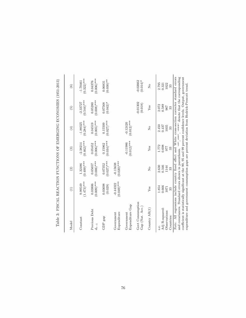
Tab

le3:

FIS

CA

LR

EA

CT

ION

FU

NC

TIO

NS

OF

EM

ER

GIN

GE

CO

NO

MIE

S(1

951-2

013)

Mod

el(1

)(2

)(3

)(4

)(5

)(6

)

Con

stant

9.9

9549

1.3

2486

-2.3

8214

-1.8

8325

-2.3

3727

-1.7

0461

(1.4

73)*

**

(0.4

09)*

**

(0.4

62)*

**

(0.2

84)*

**

(0.5

44)*

**

(0.3

22)*

**

Pre

vio

us

Deb

t0.0

3806

0.0

5657

0.0

5452

0.0

4519

0.0

5280

0.0

4376

dt−

1(0

.009)*

**

(0.0

06)*

**

(0.0

06)*

**

(0.0

05)*

**

(0.0

08)*

**

(0.0

06)*

**

GD

Pgap

0.0

3698

0.0

7352

0.1

5962

0.1

5509

0.0

7568

0.0

6831

(0.0

29)

(0.0

27)*

**

(0.0

34)*

**

(0.0

27)*

**

(0.0

42)*

(0.0

30)*

*

Gover

nm

ent

-0.4

4322

-0.1

5638

Exp

end

itu

re(0

.049)*

**

(0.0

20)*

**

Gover

nm

ent

-0.1

1986

-0.1

2420

Exp

end

itu

reG

ap

(0.0

12)*

**

(0.0

12)*

**

Govt

Con

sum

pti

on

-0.0

1302

-0.0

2662

Gap

(Nat.

Acc

.)(0

.018)

(0.0

14)*

Cou

ntr

yA

R(1

)Y

esN

oY

esN

oY

esN

o

s.e.

1.8

54

2.6

30

1.7

72

2.4

50

2.0

72

2.7

95

Ad

jR

-squ

are

d:

0.6

66

0.3

46

0.6

98

0.4

37

0.5

89

0.3

21

Ob

serv

ati

on

s:1071

1144

977

1035

967

1022

Cou

ntr

ies:

33

33

33

33

33

33

Note

:A

llre

gre

ssio

ns

incl

ud

eco

untr

yfi

xed

effec

tan

dW

hit

ecr

oss

-sec

tion

corr

ecte

rst

an

dard

erro

rsan

dco

vari

an

ces.

Sta

nd

ard

erro

rssh

ow

nin

pare

nth

esis

.“*”,“

**”,

“***”

den

ote

that

the

corr

esp

on

din

gco

effici

ent

isst

ati

stic

ally

sign

ifica

nt

at

the

90,

95

an

d99

per

cent

con

fid

ence

level

s.O

utp

ut,

gover

nm

ent

exp

end

itu

rean

dgover

nm

ent

con

sum

pti

on

gap

sare

per

cent

dev

iati

on

from

Hod

rick

-Pre

scott

tren

d.

76

Tab

le4:

FIS

CA

LR

EA

CT

ION

FU

NC

TIO

NS

FO

RA

DV

AN

CE

DA

ND

EM

ER

GIN

GE

CO

NO

MIE

S(1

951-2

013)

Mod

el(1

)(2

)(3

)(4

)(5

)(6

)

Con

stant

10.5

3960

1.5

0777

-2.2

3188

-0.6

5482

-2.2

9040

-0.5

7649

(1.5

28)*

**

(0.3

57)*

**

(0.4

00)*

**

(0.1

60)*

**

(0.4

66)*

**

(0.1

72)*

**

Pre

vio

us

Deb

t0.0

5138

0.0

2962

0.0

4576

0.0

1634

0.0

4661

0.0

1500

dt−

1(0

.007)*

**

(0.0

04)*

**

(0.0

06)*

**

(0.0

04)*

**

(0.0

06)*

**

(0.0

04)*

**

GD

Pgap

0.0

7864

0.1

2611

0.2

0956

0.2

0590

0.1

6205

0.1

5198

(0.0

31)*

*(0

.030)*

**

(0.0

43)*

**

(0.0

32)*

**

(0.0

51)*

**

(0.0

36)*

**

Gover

nm

ent

-0.4

0043

-0.0

8823

Exp

end

itu

re(0

.047)*

**

(0.0

15)*

**

Gover

nm

ent

-0.1

1558

-0.1

2788

Exp

end

itu

reG

ap

(0.0

14)*

**

(0.0

16)*

**

Govt.

Con

sum

pti

on

-0.0

3764

-0.0

7534

Gap

(Nat.

Acc

.)(0

.021)*

(0.0

20)*

**

Cou

ntr

yA

R(1

)Y

esN

oY

esN

oY

esN

o

s.e.

1.7

29

2.7

96

1.7

56

2.7

27

1.9

70

2.9

15

Ad

jR

-squ

are

d:

0.7

20

0.2

75

0.7

18

0.3

28

0.6

56

0.2

54

Ob

serv

ati

on

s:2356

2490

2195

2308

2106

2208

Cou

ntr

ies:

58

58

58

58

58

58

Note

:A

llre

gre

ssio

ns

incl

ud

eco

untr

yfi

xed

effec

tan

dW

hit

ecr

oss

-sec

tion

corr

ecte

rst

an

dard

erro

rsan

dco

vari

an

ces.

Sta

nd

ard

erro

rssh

ow

nin

pare

nth

esis

.“*”,“

**”,

“***”

den

ote

that

the

corr

esp

on

din

gco

effici

ent

isst

ati

stic

ally

sign

ifica

nt

at

the

90,

95

an

d99

per

cent

con

fid

ence

level

s.O

utp

ut,

gover

nm

ent

exp

end

itu

rean

dgover

nm

ent

con

sum

pti

on

gap

sare

per

cent

dev

iati

on

from

Hod

rick

-Pre

scott

tren

d.

77

Tab

le5:

MA

CR

OE

CO

NO

MIC

ST

AN

CE

AS

OF

2008

EU

15

GD

P-w

eig

hte

dave.

AU

TB

EL

DE

UE

SP

FR

AG

BR

ITA

NL

DP

OL

SW

EO

ther

EU

15

US

All

(a)

Macro

Aggre

gate

sτC

0.1

90.1

70.1

70.1

20.1

70.1

40.1

30.2

00.2

10.2

60.2

30.1

70.0

40.1

1τL

0.5

10.4

70.4

10.3

50.4

50.3

00.4

80.4

70.3

80.5

50.3

90.4

10.2

70.3

5τK

0.2

50.4

50.2

40.2

50.3

80.4

00.3

80.2

60.1

60.3

70.3

10.3

20.3

70.3

4

c/y

0.5

30.5

20.5

60.5

70.5

70.6

40.5

90.4

50.6

20.4

70.5

80.5

70.6

80.6

2x/y

0.2

20.2

40.1

90.2

90.2

20.1

70.2

10.2

00.2

40.2

00.2

30.2

10.2

10.2

1g/y

0.1

90.2

30.1

80.1

90.2

30.2

20.2

00.2

60.1

90.2

60.2

10.2

10.1

60.1

9tb/y

0.0

60.0

10.0

6−

0.0

6−

0.0

2−

0.0

2−

0.0

10.0

8−

0.0

40.0

7−

0.0

20.0

0−

0.0

5−

0.0

2

Rev/y

0.4

80.4

90.4

40.3

70.5

00.4

20.4

60.4

70.4

00.5

40.4

50.4

50.3

20.3

9T

ota

lE

xp/y

0.4

90.5

00.4

40.4

10.5

30.4

70.4

90.4

60.4

30.5

20.4

80.4

70.3

90.4

3

(b)

Debt

Shock

sd2007/y2007

0.3

10.7

30.4

30.1

80.3

60.2

80.8

70.2

80.1

7−

0.2

30.1

30.3

80.4

30.4

0d2011/y2011

0.4

50.8

00.5

10.4

60.6

30.6

21.0

00.3

80.3

2−

0.2

50.4

50.5

80.7

40.6

5∆d/y

0.1

40.0

70.0

90.2

80.2

70.3

30.1

40.1

00.1

5−

0.0

20.3

20.2

00.3

10.2

5

Other

isa

GD

Pweig

hted

average

ofD

enm

ark,Fin

land,G

reece,Ir

ela

nd,and

Portugal

Source:

OECD

Revenue

Statistic

s,O

ECD

Natio

nalin

com

eAccounts,and

EuroStat.

Tax

rates

are

author’s

calc

ula

tio

ns

based

on

Mendoza,Razin

,and

Tesar

(1994).“

TotalExp”

istotal

non-interest

governm

ent

outla

ys.

78

Tab

le6:

PA

RA

ME

TE

RV

AL

UE

S

Pre

fere

nces:

US

EU

15

Sourc

esβ

dis

count

fact

or

0.9

98

stea

dy

state

Eule

req

uati

on

for

capit

al

σri

skav

ersi

on

2.0

00

standard

DSG

Eva

lue

ala

bor

supply

elast

icit

y2.6

75

l=

0.1

8(P

resc

ott

,2004)

Tech

nolo

gy:

αla

bor

inco

me

share

0.6

1(T

rabandt

and

Uhlig,

2011)

γgro

wth

rate

0.0

038

real

GD

Pp.c

.gro

wth

of

sam

ple

countr

ies

(Euro

stat

1995–2011)

ηca

pit

al

adju

stm

ent

cost

2E

last

icit

yof

capit

al

tax

base

(Gru

ber

and

Rauh,

2007,

Dw

enger

and

Ste

iner

,2012)

mca

paci

tyuti

liza

tion

1st

eady

state

norm

aliza

tion

δ(m

)dep

reci

ati

on

rate

0.0

163

capit

al

law

of

moti

on,x/y

=0.1

9,k/y

=2.6

2(O

EC

D,

AM

EC

O)

χ0

δ(m

)co

effici

ent

0.0

23

0.0

24

opti

mality

condit

ion

for

uti

liza

tion

giv

enδ(m

),m

χ1

δ(m

)ex

ponen

t1.4

41.4

5se

tto

yie

ldδ(m

)=

0.0

164

ωco

untr

ysi

ze0.4

60.5

4G

DP

share

inall

sam

ple

countr

ies

Fis

cal

Policy:

g/y

Gov

’tex

psh

are

inG

DP

0.1

60.2

1O

EC

DN

ati

onal

Inco

me

Acc

ounts

τ Cco

nsu

mpti

on

tax

0.0

40.1

7M

RT

modifi

edτ L

lab

or

inco

me

tax

0.2

70.4

1M

RT

modifi

edτ K

capit

al

inco

me

tax

0.3

70.3

2M

RT

modifi

edθ

dep

reci

ati

on

allow

ance

lim

itati

on

0.2

0(REVcorp

K/REVK

)(KNR/K

),O

EC

DR

even

ue

Sta

tist

ics

and

EU

KL

EM

S

Note

:T

he

implied

gro

wth

adju

sted

dis

count

facto

rβ

is0.9

95,

and

the

implied

pre

-cri

sis

annual

inte

rest

rate

is3.8

%.REV

corp

K/REVK

isth

e

rati

oof

corp

ora

teta

xre

venue

toto

tal

capit

al

tax

revenue.K

NR/K

isth

era

tio

of

nonre

sidenti

al

fixed

capit

al

toto

tal

fixed

capit

al.

79

Table 7: BALANCED GROWTH ALLOCATIONS (GDP RATIOS) OF 2008

US EU15

Data Model Data Modelc/y 0.68 0.63 0.57 0.56i/y 0.21 0.21 0.21 0.23g/y∗ 0.16 0.16 0.21 0.21

tb/y −0.05 0.00 0.00 0.00Rev/y 0.32 0.32 0.45 0.46d/y∗ 0.76 0.76 0.60 0.60

80

Tab

le8:

MA

CR

OE

CO

NO

MIC

EF

FE

CT

SO

FA

NIN

CR

EA

SE

INU

SC

AP

ITA

LT

AX

RA

TE

(The

EU

15

main

tain

sre

ven

ue

neu

trality

wit

hla

bor

tax)

Op

enE

conom

yC

lose

dE

conom

y

US

EU

15

US

Tax

rate

sO

ldN

ewO

ldN

ewO

ldN

ew

τ K0.3

70.4

00.3

20.3

20.3

70.4

0τ C

0.0

40.0

40.1

70.1

70.0

40.0

4τ L

0.2

70.2

70.4

10.4

00.2

70.2

7

PV

of

fisc

al

defi

cit

over

1.3

70.0

06.1

6pre

-cri

sis

GD

Pas

per

centa

ge

poin

tch

ange

from

ori

gin

al

ss

Welf

are

eff

ects

(perc

ent)

Ste

ady-s

tate

gain

−2.2

70.5

9−

2.5

5O

ver

al

gain

−2.1

90.7

4−

2.2

2

Per

centa

ge

changes

Impact

Eff

ect

Long-R

un

Eff

ect

Impact

Eff

ect

Long-R

un

Eff

ect

Impact

Eff

ect

Long-R

un

Eff

ect

y−

1.2

3−

3.8

7−

0.1

51.2

5−

2.3

5−

3.5

7c

−1.8

7−

2.8

31.4

41.2

8−

1.5

3−

2.9

1k

0.0

0−

7.6

10.0

01.2

50.0

0−

7.3

2

Per

centa

ge

poin

tch

anges

tb/y

3.2

1−

0.3

0−

2.7

00.2

4i/y

−3.0

1−

1.0

21.7

70.0

0−

0.9

1−

1.0

2r

−0.0

0−

0.0

0−

0.0

0−

0.0

0−

0.0

0−

0.0

0l

0.1

1−

0.1

7−

0.0

10.2

1−

0.1

3−

0.1

1m

−4.2

3−

0.8

66

−0.3

15

−0.0

00

−5.2

77

−0.8

66

81

Tab

le9:

MA

CR

OE

CO

NO

MIC

EF

FE

CT

SO

FA

DE

CR

EA

SE

INE

U15

CA

PIT

AL

TA

XR

AT

E

(The

U.S

main

tain

sre

ven

ue

neu

trality

wit

hla

bor

tax)

Op

enE

conom

yC

lose

dE

conom

y

US

EU

15

EU

15

Tax

rate

sO

ldN

ewO

ldN

ewO

ldN

ew

τ K0.3

70.3

70.3

20.2

00.3

70.3

7τ C

0.0

40.0

40.1

70.1

70.0

40.1

7τ L

0.2

70.2

80.4

10.4

10.2

70.4

1

PV

of

fisc

al

defi

cit

over

-0.0

022.3

49.6

2pre

-cri

sis

GD

Pas

per

centa

ge

poin

tch

ange

from

ori

gin

al

ss

Welf

are

eff

ects

(perc

ent)

Ste

ady-s

tate

gain

0.3

67.3

57.9

3O

ver

al

gain

−0.2

36.8

66.9

9

Per

centa

ge

changes

Impact

Eff

ect

Long-R

un

Eff

ect

Impact

Eff

ect

Long-R

un

Eff

ect

Impact

Eff

ect

Long-R

un

Eff

ect

y2.3

0−

1.4

06.0

512.7

78.3

811.9

9c

−1.5

9−

0.6

45.8

29.0

35.1

49.1

9k

0.0

0−

1.5

00.0

026.1

00.0

025.2

3

Per

centa

ge

poin

tch

anges

tb/y

8.9

2−

0.7

5−

6.5

70.5

6i/y

−5.6

40.0

08.1

83.6

63.3

13.6

6r

0.0

0−

0.0

00.0

0−

0.0

00.0

0−

0.0

0l

0.4

7−

0.3

10.0

50.4

80.4

30.3

6m

2.3

40.0

012.9

33.3

114.9

43.3

1

82

Tab

le10

:M

AC

RO

EC

ON

OM

ICE

FF

EC

TS

OF

AN

INC

RE

ASE

INT

HE

U.S

.L

AB

OR

TA

XR

AT

E

(The

EU

15

main

tain

sre

ven

ue

neu

trality

wit

hla

bor

tax)

US

EU

15

US

Tax

rate

sO

ldN

ewO

ldN

ewO

ldN

ew

τ K0.3

70.3

70.3

20.3

20.3

70.3

7τ C

0.0

40.0

40.1

70.1

70.0

40.0

4τ L

0.2

70.2

90.4

10.4

10.2

70.2

9

PV

of

fisc

al

defi

cit

over

31.0

00.0

031.9

5pre

-cri

sis

GD

Pas

per

centa

ge

poin

tch

ange

from

ori

gin

al

ss

Welf

are

eff

ects

(perc

ent)

Ste

ady-s

tate

gain

−0.9

20.1

5−

0.9

8O

ver

al

gain

−0.9

00.1

8−

0.9

1

Per

centa

ge

changes

Impact

Eff

ect

Long-R

un

Eff

ect

Impact

Eff

ect

Long-R

un

Eff

ect

Impact

Eff

ect

Long-R

un

Eff

ect

y−

1.1

6−

1.7

5−

0.0

20.3

0−

1.4

1−

1.6

8c

−1.8

8−

2.0

90.3

40.3

1−

1.8

0−

2.1

0k

0.0

0−

1.7

50.0

00.3

00.0

0−

1.6

8

Per

centa

ge

poin

tch

anges

tb/y

0.7

2−

0.0

7−

0.6

10.0

6i/y

−0.4

60.0

00.4

00.0

00.0

2−

0.0

0r

−0.0

0−

0.0

0−

0.0

0−

0.0

0−

0.0

0−

0.0

0l

−0.2

9−

0.3

50.0

00.0

5−

0.3

5−

0.3

4m

−0.7

30.0

0−

0.0

6−

0.0

0−

0.9

60.0

0

83

Tab

le11

:M

AC

RO

EC

ON

OM

ICE

FF

EC

TS

OF

AN

INC

RE

ASE

INT

HE

EU

15

LA

BO

RT

AX

RA

TE

(The

U.S

.m

ain

tain

sre

ven

ue

neu

trality

wit

hla

bor

tax)

US

EU

15

EU

15

Tax

rate

sO

ldN

ewO

ldN

ewO

ldN

ew

τ K0.3

70.3

70.3

20.3

20.3

70.3

7τ C

0.0

40.0

40.1

70.1

70.0

40.1

7τ L

0.2

70.2

70.4

10.4

70.2

70.4

7

PV

of

fisc

al

defi

cit

over

0.0

011.7

516.0

2pre

-cri

sis

GD

Pas

per

centa

ge

poin

tch

ange

from

ori

gin

al

ss

Welf

are

eff

ects

(perc

ent)

Ste

ady-s

tate

gain

−0.1

2−

5.0

4−

5.1

9O

ver

al

gain

0.0

7−

4.9

1−

4.9

2

Per

centa

ge

changes

Impact

Eff

ect

Long-R

un

Eff

ect

Impact

Eff

ect

Long-R

un

Eff

ect

Impact

Eff

ect

Long-R

un

Eff

ect

y−

0.6

80.4

1−

4.2

8−

6.2

0−

5.0

6−

5.9

9c

0.4

50.1

6−

7.3

5−

8.1

8−

7.1

3−

8.2

2k

0.0

00.4

10.0

0−

6.2

00.0

0−

5.9

9

Per

centa

ge

poin

tch

anges

tb/y

−2.4

70.2

22.1

6−

0.2

0i/y

1.6

4−

0.0

0−

1.2

9−

0.0

00.1

1−

0.0

0r

−0.0

0−

0.0

0−

0.0

0−

0.0

0−

0.0

0−

0.0

0l

−0.1

40.0

8−

0.9

0−

1.0

5−

1.0

4−

1.0

1m

−0.6

7−

0.0

0−

2.8

70.0

0−

3.5

9−

0.0

0

84

Tab

le12

:SH

OR

T-R

UN

EL

AST

ICIT

YO

FU

SC

AP

ITA

LT

AX

BA

SE

Ela

stic

ity

y 1l 1

m1

Em

pir

ical

esti

mat

es[0

.1,

0.5

]

Mod

elIm

pli

cati

ons

for

the

U.S

.ex

og.

uti

liza

tion

&θ

=1

−0.0

90.0

4%

0.0

11

exog

.u

tili

zati

on&θ

=0.

2−

0.0

90.0

8%

0.0

28

end

og.

uti

liza

tion

&θ

=0.

20.2

9−

0.15%

0.0

10

−0.

471

Mod

elIm

pli

cati

ons

for

the

EU

15

exog

.u

tili

zati

on&θ

=1

−0.0

40.0

1%

0.0

04

exog

.u

tili

zati

on&θ

=0.

2−

0.0

20.0

3%

0.0

08

end

og.

uti

liza

tion

&θ

=0.

20.3

2−

0.14%

0.0

04

−0.

393

Note

:E

last

icit

yis

measu

red

as

the

perc

enta

ge

decre

ase

of

capit

alta

xbase

inth

efirs

tyear

aft

er

a1%

incre

ase

inth

ecapit

al

tax

rate

isin

troducede.

For

em

pir

ical

est

imate

s,se

eG

rub

er

and

Rauh

(2007)

and

Dw

enger

and

Ste

iner

(2012).y1

andm

1pro

vid

es

the

perc

ent

devia

tion

from

the

init

ial

steady

state

inth

eim

pact

year.l 1

denote

sth

ep

erc

enta

ge

poin

tsch

ange

from

the

init

ial

steady

state

.

85

Table 13: Model Parameters

Parameter ValueDiscount Factor β 0.96Risk Aversion σ 1.00Avg. Income y 0.79Low household wealth bL0 0.00Avg. Gov. Consumption µg 0.18Autocorrel. G ρg 0.88Std Dev Error σg 0.017Initial Gov. Debt B0 0.79Output Cost Default φ0 0.02

Note: Government expenditures, income and debt values are derived

using Eurostat data for France, Germany, Greece, Ireland, Italy, Spain and Portugal.

Table 14: Euro Area: Key Fiscal Statistics and Wealth Inequality

Gov. Debt Gov. Exp. Spreads GiniMoment (%) Avg. 2011 Avg. “crisis peak” Avg. “crisis peak” WealthFrance 34.87 62.72 23.40 24.90 0.08 1.04 0.73Germany 33.34 52.16 18.80 20.00 - - 0.67Greece 84.25 133.09 18.40 23.60 0.37 21.00 0.65Ireland 14.07 64.97 16.10 20.50 0.11 6.99 0.58Italy 95.46 100.22 19.40 21.40 0.27 3.99 0.61Portugal 35.21 75.83 20.00 22.10 0.20 9.05 0.67Spain 39.97 45.60 17.60 21.40 0.13 4.35 0.57Avg. 48.17 76.37 19.10 21.99 0.22 7.74 0.64Median 35.21 64.97 18.80 21.40 0.17 5.67 0.65

Note: Author’s calculations are based on OECD Statistics, Eurostat, ECSB and Davies, S., Shorrocks, and Wolff (2009).

“Gov. Debt” refers to Total General Government Net Financial Liabilities (avg 1990-2007); “Gov. Exp.” corresponds to

government purchases in National Accounts (avg 2000-2007); “Sov Spreads” correspond to the difference between interest rates

of the given country and Germany for bonds of similar maturity (avg 2000-2007). For a given country i, they are computed as

(1 + ri)/(1 + rGer)− 1. “Crisis Peak” refers to the maximum value observed during 2008-2012 using data from Eurostat. “Gini

Wealth” are Gini wealth coefficients for 2000 from Davies, S., Shorrocks, and Wolff (2009) Appendix V.

86