Embed Size (px)
Citation preview
ANOVA_EXAMPLE P60 Brainerd 1
What If There Are More Than Two Factor Levels?
• Chapter 3
• Comparing more that two factor levels…the analysis of variance
• ANOVA decomposition of total variability• Statistical testing & analysis • Checking assumptions, model validity • Post-ANOVA testing of means
ANOVA_EXAMPLE P60 Brainerd 2
What If There Are More Than Two Factor Levels?
• The t-test does not directly apply• There are lots of practical situations where there are either
more than two levels of interest, or there are several factors of simultaneous interest
• The analysis of variance (ANOVA) is the appropriate analysis “engine” for these types of experiments – Chapter 3, textbook
• The ANOVA was developed by Fisher in the early 1920s, and initially applied to agricultural experiments
• Used extensively today for industrial experiments
ANOVA_EXAMPLE P60 Brainerd 3
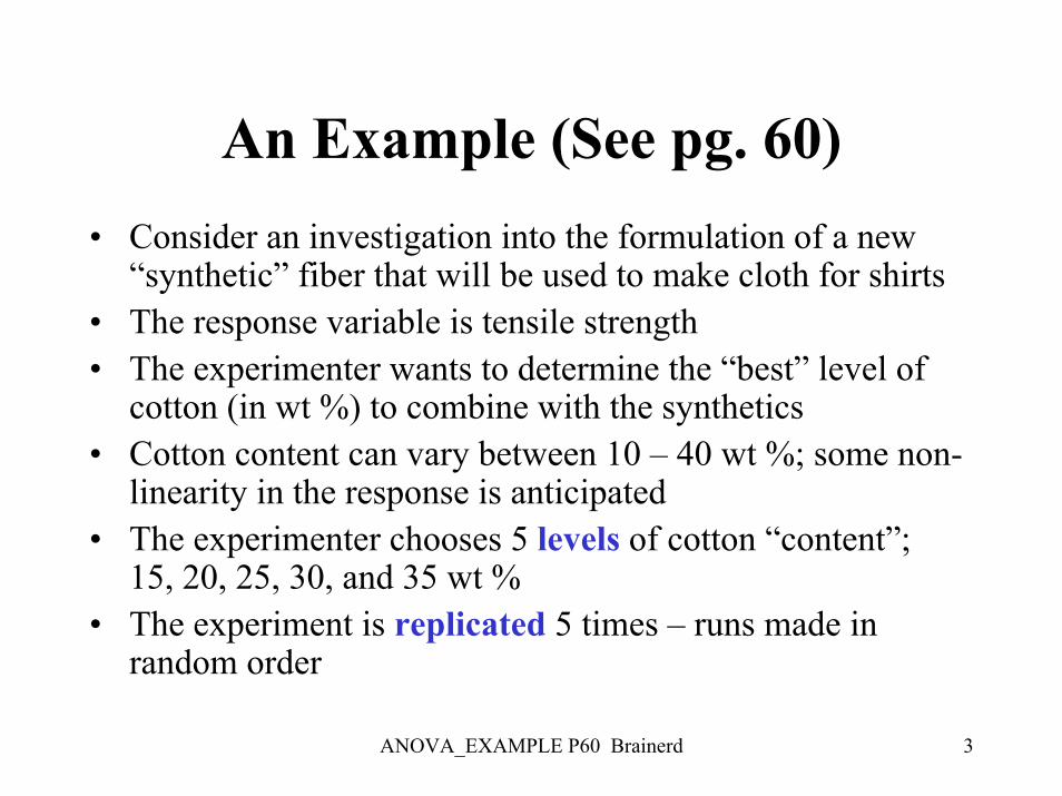
An Example (See pg. 60)• Consider an investigation into the formulation of a new
“synthetic” fiber that will be used to make cloth for shirts• The response variable is tensile strength• The experimenter wants to determine the “best” level of
cotton (in wt %) to combine with the synthetics• Cotton content can vary between 10 – 40 wt %; some non-
linearity in the response is anticipated• The experimenter chooses 5 levels of cotton “content”;
15, 20, 25, 30, and 35 wt %• The experiment is replicated 5 times – runs made in
random order
ANOVA_EXAMPLE P60 Brainerd 4
ANOVA: Design of ExperimentsChapter 3
A product development engineer is interested in investigating the tensile strength of a new synthetic fiber that will be used to make men’s shirts.
A product development engineer is interested in investigating the tensile strength of a new synthetic fiber that will be used to make men’s shirts. The engineer knows from previous experience that the strength is affected by the weight percent of cotton used in the blend of materials for the fiber.
A product development engineer is interested in investigating the tensile strength of a new synthetic fiber that will be used to make men’s shirts. The engineer knows from previous experience that the strength is affected by the weight percent of cotton used in the blend of materials for the fiber. Furthermore, he suspects that increasing the cotton content will increase thestrength, at least initially.
A product development engineer is interested in investigating the tensile strength of a new synthetic fiber that will be used to make men’s shirts. The engineer knows from previous experience that the strength is affected by the weight percent of cotton used in the blend of materials for the fiber. Furthermore, he suspects that increasing the cotton content will increase the strength, at least initially. He also knows that cotton content should range between about 10 percent and 40 percent if the final cloth is to have other quality characteristics that are desired. The engineer decides to test specimens at five levels of cotton weight percent: 15 percent, 20 percent, 25 percent, 30 percent, and 35 percent.
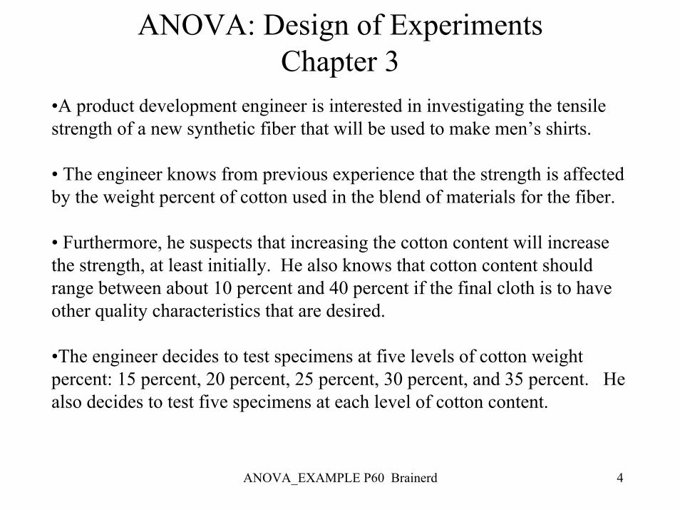
•A product development engineer is interested in investigating the tensile strength of a new synthetic fiber that will be used to make men’s shirts.
• The engineer knows from previous experience that the strength is affected by the weight percent of cotton used in the blend of materials for the fiber.
• Furthermore, he suspects that increasing the cotton content will increase the strength, at least initially. He also knows that cotton content should range between about 10 percent and 40 percent if the final cloth is to have other quality characteristics that are desired.
•The engineer decides to test specimens at five levels of cotton weight percent: 15 percent, 20 percent, 25 percent, 30 percent, and 35 percent. He also decides to test five specimens at each level of cotton content.
ANOVA_EXAMPLE P60 Brainerd 5
ANOVA: Design of ExperimentsChapter 3
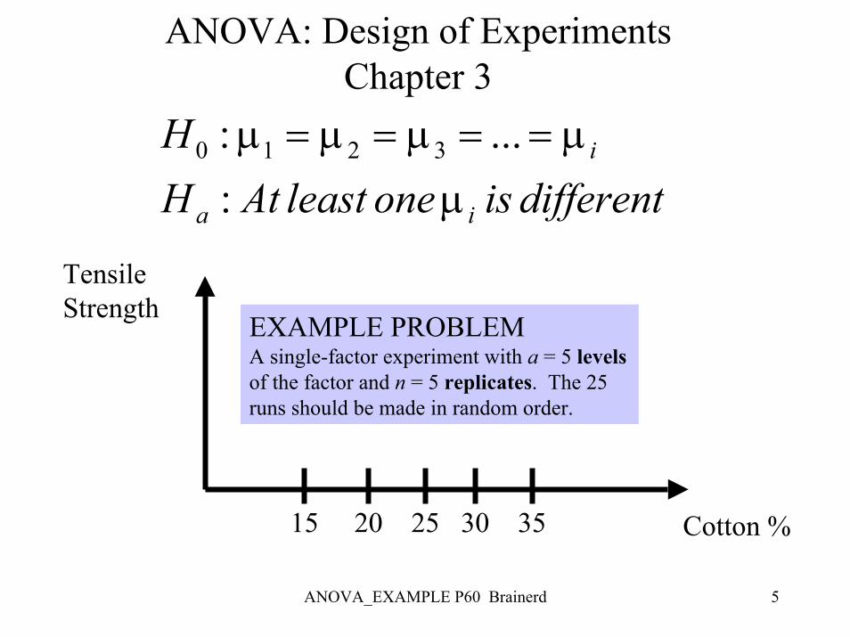
differentisoneleastAtHH
ia
i
µµµµµ
:...: 3210 ====
TensileStrength
EXAMPLE PROBLEMA single-factor experiment with a = 5 levels of the factor and n = 5 replicates. The 25 runs should be made in random order.
15 20 25 30 35 Cotton %
ANOVA_EXAMPLE P60 Brainerd 6
ANOVA: Design of ExperimentsChapter 3
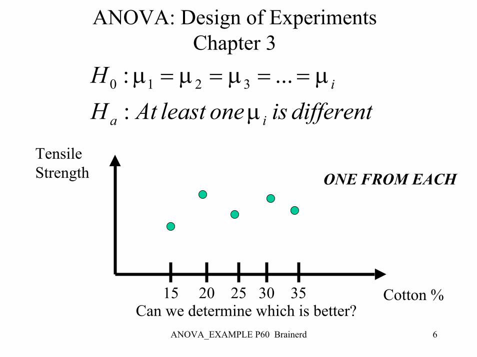
differentisoneleastAtHH
ia
i
µµµµµ
:...: 3210 ====
TensileStrength ONE FROM EACH
15 20 25 30 35Can we determine which is better?
Cotton %

ANOVA_EXAMPLE P60 Brainerd 7
ANOVA: Design of ExperimentsChapter 3
REPLICATIONdifferentisoneleastAtH
H
ia
i
µµµµµ
:...: 3210 ====
TensileStrength
15 20 25 30 35 Cotton %What does replication provide?
ANOVA_EXAMPLE P60 Brainerd 8
ANOVA: Design of ExperimentsChapter 3
Cotton %
TensileStrength
15 20 25 30 35
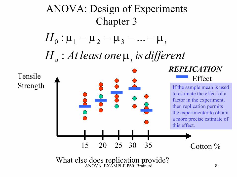
REPLICATIONEffect
differentisoneleastAtHH
ia
i
µµµµµ
:...: 3210 ====
If the sample mean is used to estimate the effect of a factor in the experiment, then replication permits the experimenter to obtain a more precise estimate of this effect.
What else does replication provide?
ANOVA_EXAMPLE P60 Brainerd 9
ANOVA: Design of ExperimentsChapter 3
Cotton %
TensileStrength
15 20 25 30 35
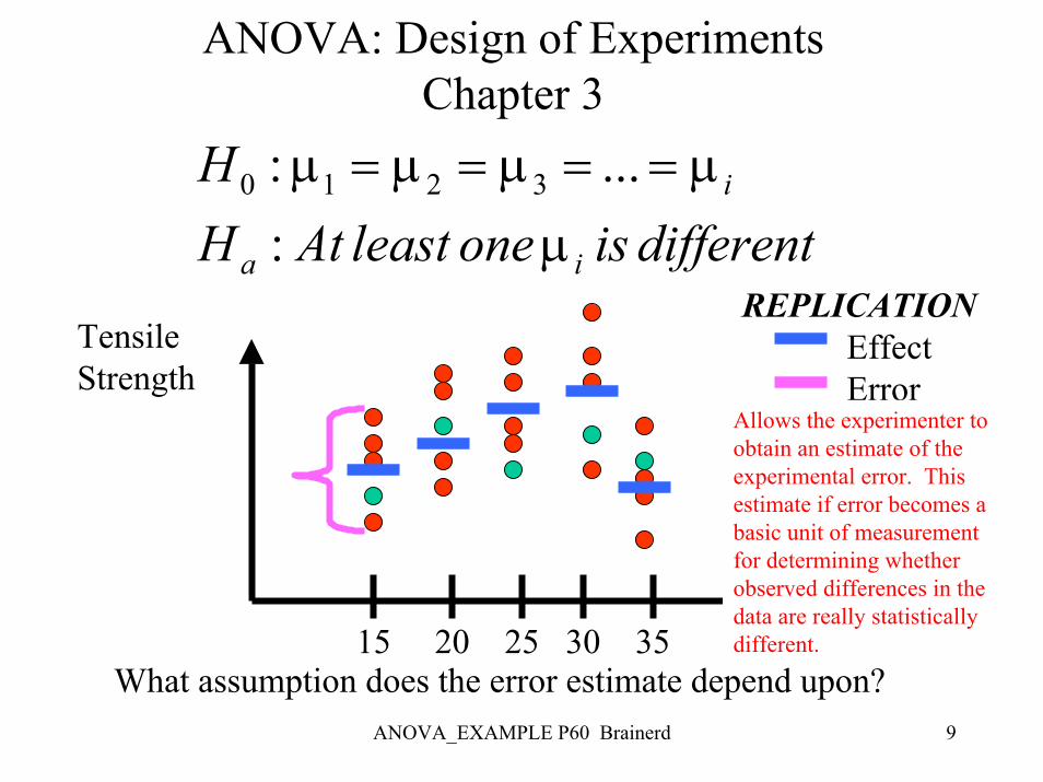
REPLICATIONEffectError
nix
22 σ
σ =
What assumption does the error estimate depend upon?
differentisoneleastAtHH
ia
i
µµµµµ
:...: 3210 ====
Allows the experimenter to obtain an estimate of the experimental error. This estimate if error becomes a basic unit of measurement for determining whether observed differences in the data are really statistically different.
ANOVA_EXAMPLE P60 Brainerd 10
ANOVA: Design of ExperimentsChapter 3
15 20 25 30 35
REPLICATIONEffectError
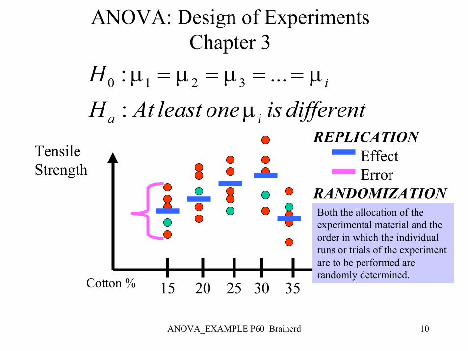
RANDOMIZATION
differentisoneleastAtHH
ia
i
µµµµµ
:...: 3210 ====
Both the allocation of the experimental material and the order in which the individual runs or trials of the experiment are to be performed are randomly determined.
TensileStrength
Cotton %
ANOVA_EXAMPLE P60 Brainerd 11
ANOVA: Design of ExperimentsChapter 3
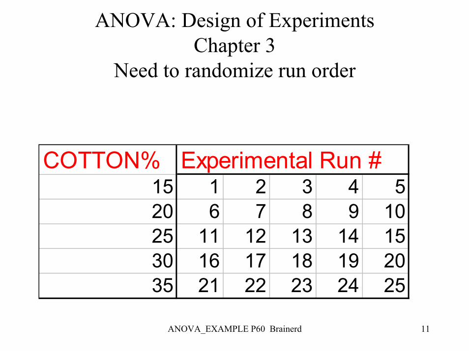
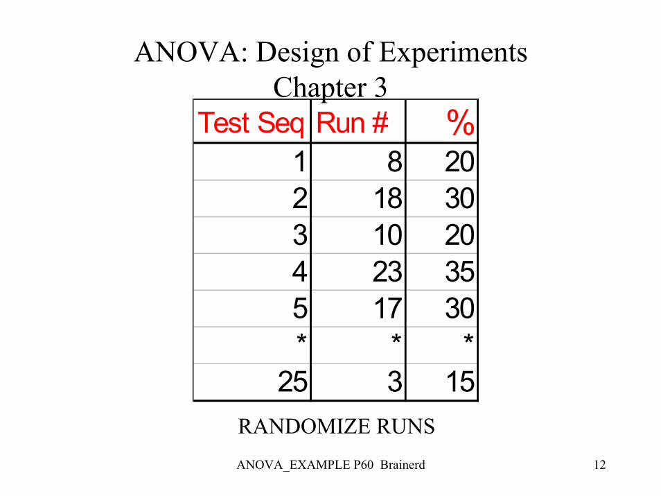
Need to randomize run order
COTTON% Experimental Run #15 1 2 3 4 520 6 7 8 9 1025 11 12 13 14 1530 16 17 18 19 2035 21 22 23 24 25
ANOVA_EXAMPLE P60 Brainerd 12
ANOVA: Design of ExperimentsChapter 3
Test Seq Run # %1 8 202 18 303 10 204 23 355 17 30* * *
25 3 15RANDOMIZE RUNS
ANOVA_EXAMPLE P60 Brainerd 13
ANOVA: Design of ExperimentsChapter 3
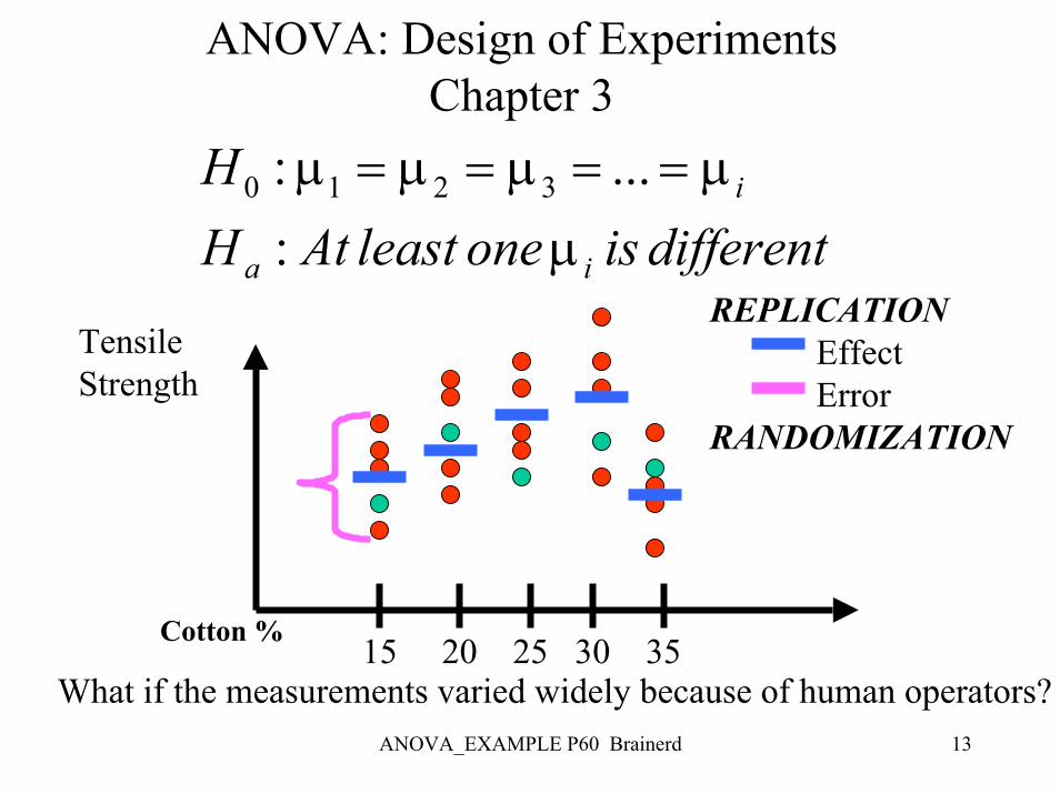
REPLICATIONEffectError
RANDOMIZATION
differentisoneleastAtHH
ia
i
µµµµµ
:...: 3210 ====
TensileStrength
Cotton % 15 20 25 30 35What if the measurements varied widely because of human operators?
ANOVA_EXAMPLE P60 Brainerd 14
ANOVA: Design of ExperimentsChapter 3
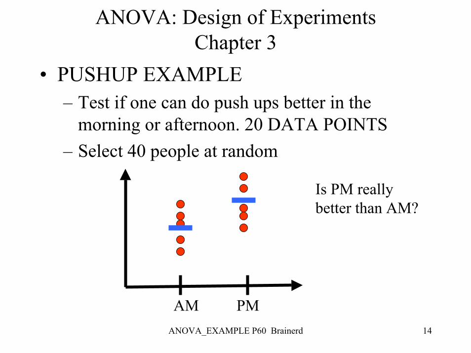
• PUSHUP EXAMPLE– Test if one can do push ups better in the
morning or afternoon. 20 DATA POINTS– Select 40 people at random
AM PM
Is PM really better than AM?
ANOVA_EXAMPLE P60 Brainerd 15
ANOVA: Design of ExperimentsChapter 3
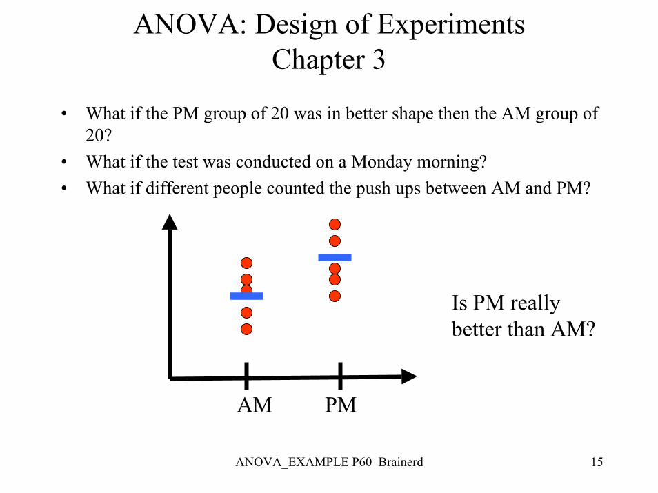
• What if the PM group of 20 was in better shape then the AM group of 20?
• What if the test was conducted on a Monday morning?• What if different people counted the push ups between AM and PM?
AM PM
Is PM really better than AM?
ANOVA_EXAMPLE P60 Brainerd 16
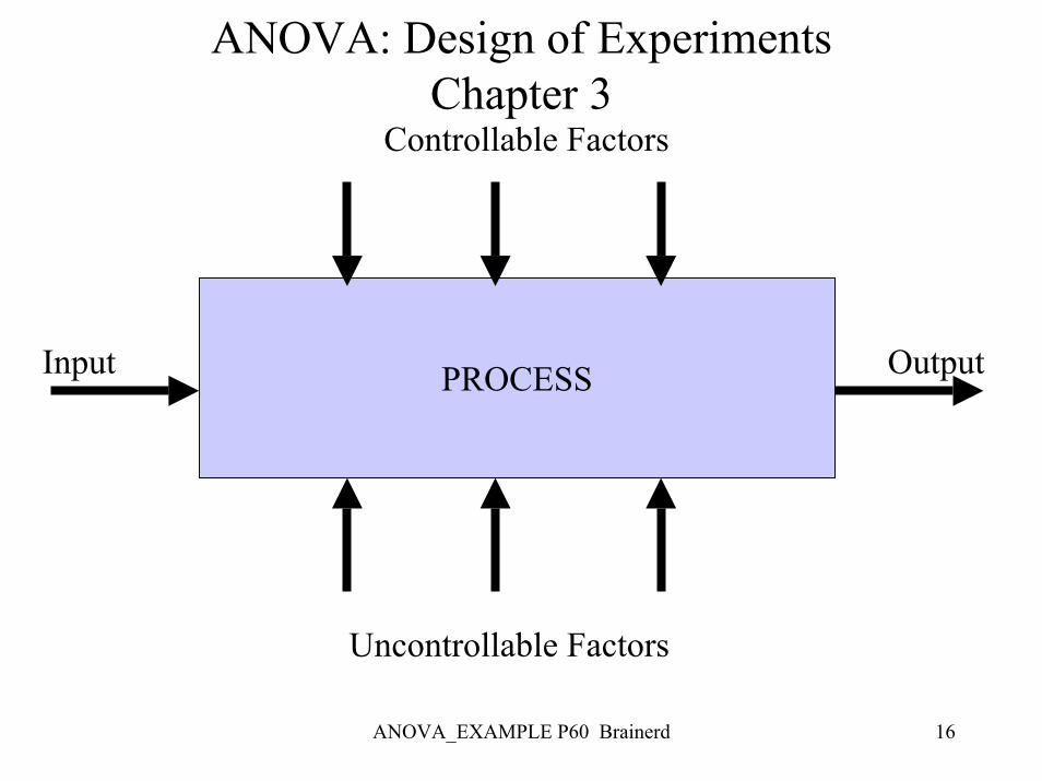
ANOVA: Design of ExperimentsChapter 3
Controllable Factors
PROCESSInput Output
Uncontrollable Factors
ANOVA_EXAMPLE P60 Brainerd 17
ANOVA: Design of ExperimentsChapter 3
• BLOCKING– Used to limit the uncontrollable factors– Therefore increase precision
• PUSH UP EXAMPLE– Paired Data = BLOCKING– Have same person do AM and PM– You are investigating AM vs PM not which group can
do more pushups.– Randomly Sort experiment by Days of the Week and
have one grader
ANOVA_EXAMPLE P60 Brainerd 18
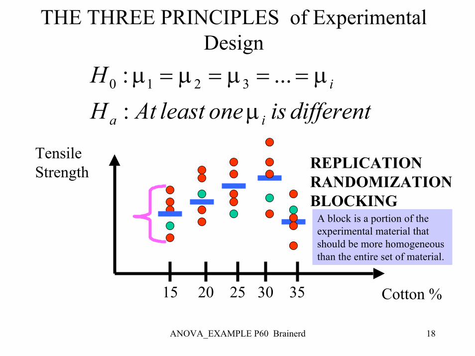
THE THREE PRINCIPLES of Experimental Design
differentisoneleastAtHH
ia
i
µµµµµ
:...: 3210 ====
TensileStrength REPLICATION
RANDOMIZATIONBLOCKING
Cotton %15 20 25 30 35
A block is a portion of the experimental material that should be more homogeneous than the entire set of material.

ANOVA_EXAMPLE P60 Brainerd 19
Analysis of Variance (ANOVA)
differentisoneleastAtHH
ia
i
µµµµµ
:...: 3210 ====
Cotton %
TensileStrength
15 20 25 30 35VariationWithin Samples
VariationBetween Samples

ANOVA_EXAMPLE P60 Brainerd 20
Analysis of Variance (ANOVA)
Cotton %
TensileStrength
15 20 25 30 35
When very different
Between Sample Variation LargeWithin Sample Variation Small
ANOVA_EXAMPLE P60 Brainerd 21
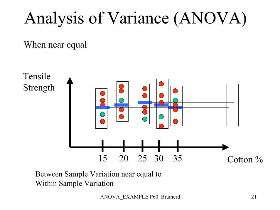
Analysis of Variance (ANOVA)When near equal
TensileStrength
Cotton %15 20 25 30 35Between Sample Variation near equal toWithin Sample Variation
ANOVA_EXAMPLE P60 Brainerd 22
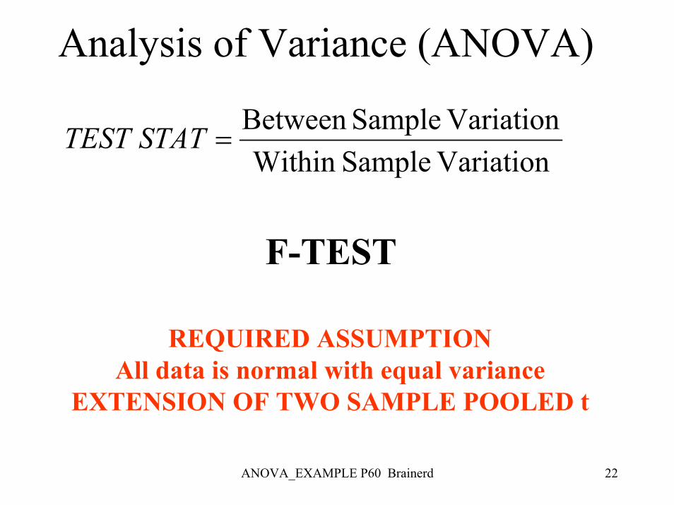
Analysis of Variance (ANOVA)
Variation SampleWithin Variation SampleBetween
=STATTEST
F-TEST
REQUIRED ASSUMPTIONAll data is normal with equal variance
EXTENSION OF TWO SAMPLE POOLED t

ANOVA_EXAMPLE P60 Brainerd 23
Analysis of Variance (ANOVA)SETUP (i = factor; j = replicate)
Level Replicates Mean SD
1 2 3 * j1 11 12 13 * 1j 1*2 21 22 23 * 2j 2*3 31 32 33 * 3j 3** * * * * *i i1 i2 i3 * ij
**
tmeasuremen jlevel, i valueobserved thth, =jix
ANOVA_EXAMPLE P60 Brainerd 24
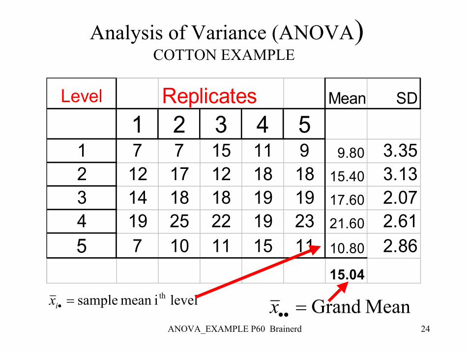
Analysis of Variance (ANOVA)COTTON EXAMPLE
Level Replicates Mean SD
1 2 3 4 51 7 7 15 11 9 9.80 3.352 12 17 12 18 18 15.40 3.133 14 18 18 19 19 17.60 2.074 19 25 22 19 23 21.60 2.615 7 10 11 15 11 10.80 2.86
15.04
level imean sample th=•ix Mean Grand=••x
ANOVA_EXAMPLE P60 Brainerd 25
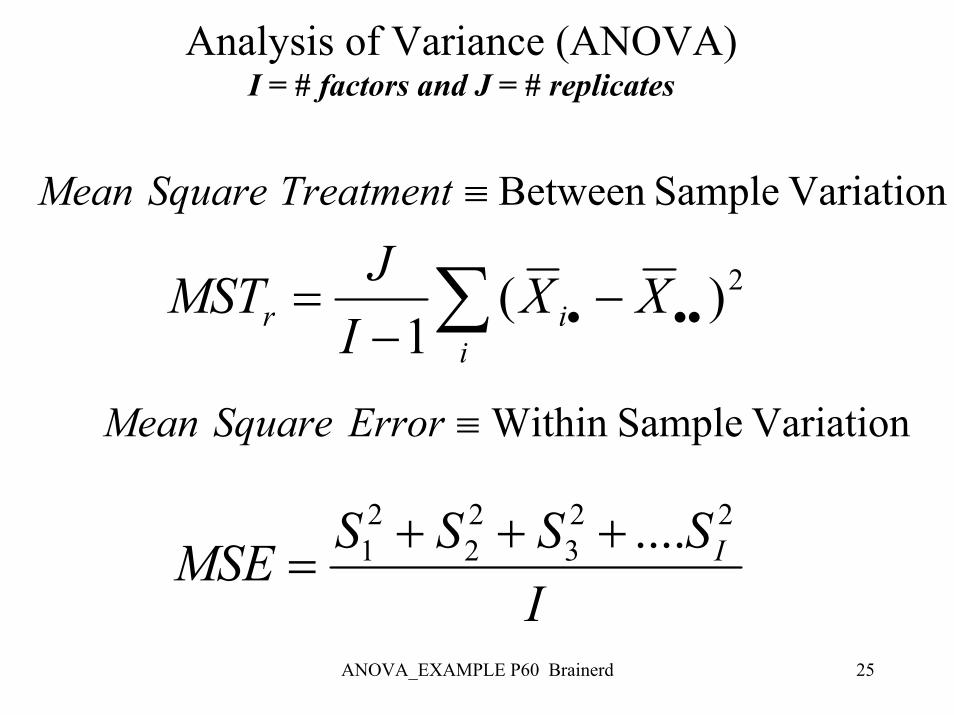
Analysis of Variance (ANOVA)I = # factors and J = # replicates
Variation SampleBetween ≡TreatmentSquareMean
∑ ••• −−=
iir XX
IJMST 2)(
1Variation SampleWithin ≡ErrorSquareMean
ISSSSMSE I
223
22
21 ....+++
=
ANOVA_EXAMPLE P60 Brainerd 26
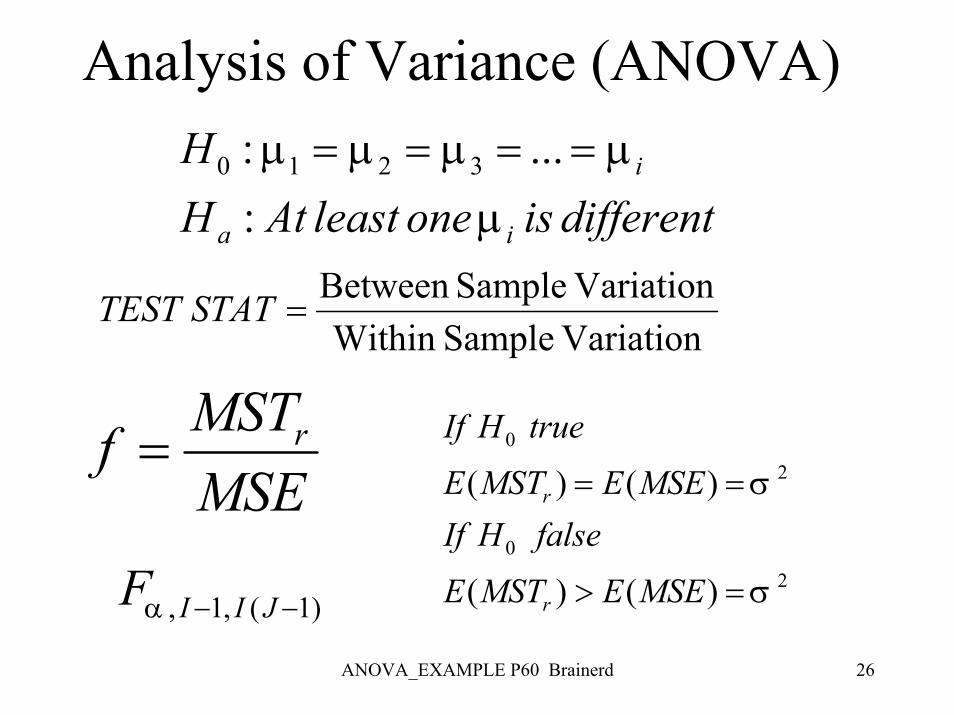
Analysis of Variance (ANOVA)
differentisoneleastAtHH
ia
i
µµµµµ
:...: 3210 ====
Variation SampleWithin Variation SampleBetween
=STATTEST
MSEMSTf r=
20
20
)()(
)()(
σ
σ
=>
==
MSEEMSTE
falseHIfMSEEMSTE
trueHIf
r
r
)1(,1, −− JIIFα
ANOVA_EXAMPLE P60 Brainerd 27
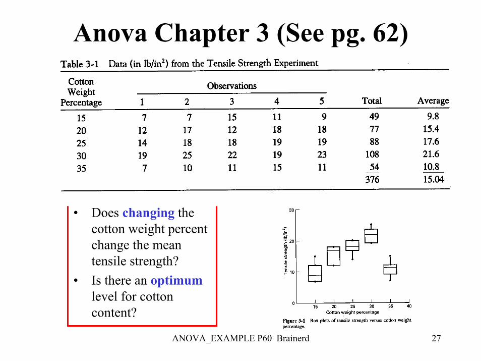
Anova Chapter 3 (See pg. 62)
• Does changing the cotton weight percent change the mean tensile strength?
• Is there an optimumlevel for cotton content?
ANOVA_EXAMPLE P60 Brainerd 28
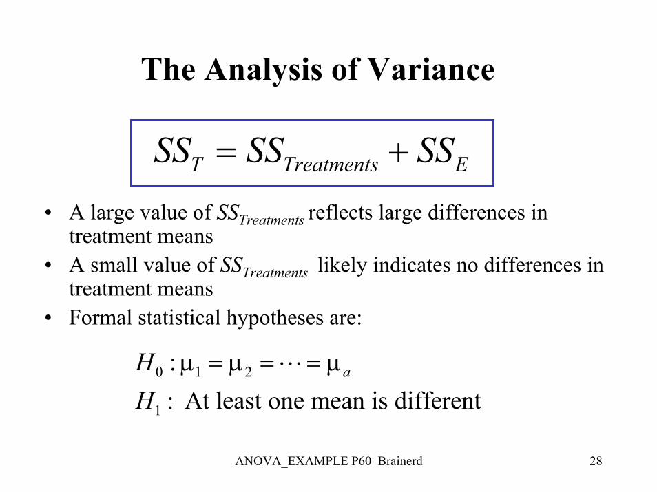
The Analysis of Variance
T Treatments ESS SS SS= +
• A large value of SSTreatments reflects large differences in treatment means
• A small value of SSTreatments likely indicates no differences in treatment means
• Formal statistical hypotheses are:
0 1 2
1
:: At least one mean is different
aHH
µ µ µ= = =L
ANOVA_EXAMPLE P60 Brainerd 29
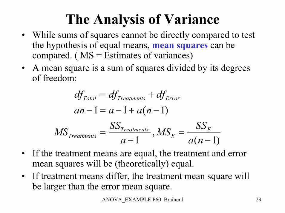
The Analysis of Variance• While sums of squares cannot be directly compared to test
the hypothesis of equal means, mean squares can be compared. ( MS = Estimates of variances)
• A mean square is a sum of squares divided by its degrees of freedom:
• If the treatment means are equal, the treatment and error mean squares will be (theoretically) equal.
• If treatment means differ, the treatment mean square will be larger than the error mean square.
1 1 ( 1)
,1 ( 1)
Total Treatments Error
Treatments ETreatments E
df df dfan a a n
SS SSMS MSa a n
= +− = − + −
= =− −
ANOVA_EXAMPLE P60 Brainerd 30
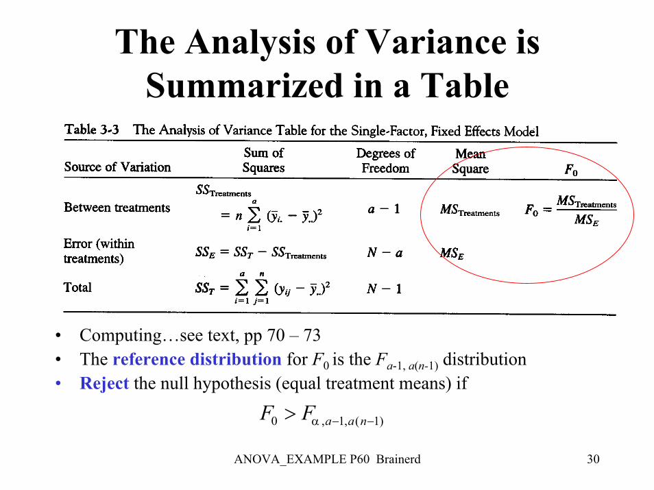
The Analysis of Variance is Summarized in a Table
• Computing…see text, pp 70 – 73• The reference distribution for F0 is the Fa-1, a(n-1) distribution• Reject the null hypothesis (equal treatment means) if
0 , 1, ( 1)a a nF Fα − −>
ANOVA_EXAMPLE P60 Brainerd 31
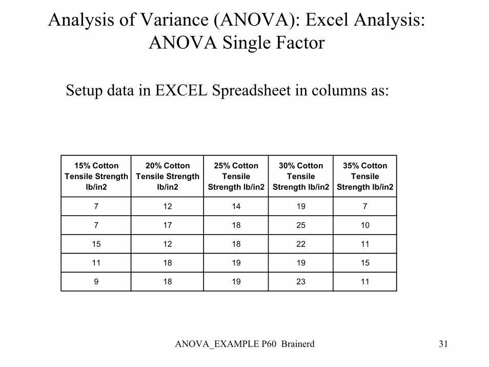
Analysis of Variance (ANOVA): Excel Analysis: ANOVA Single Factor
Setup data in EXCEL Spreadsheet in columns as:
15% Cotton Tensile Strength
lb/in2
20% Cotton Tensile Strength
lb/in2
25% Cotton Tensile
Strength lb/in2
30% Cotton Tensile
Strength lb/in2
35% Cotton Tensile
Strength lb/in2
7 12 14 19 7
7 17 18 25 10
15 12 18 22 11
11 18 19 19 15
9 18 19 23 11
ANOVA_EXAMPLE P60 Brainerd 32
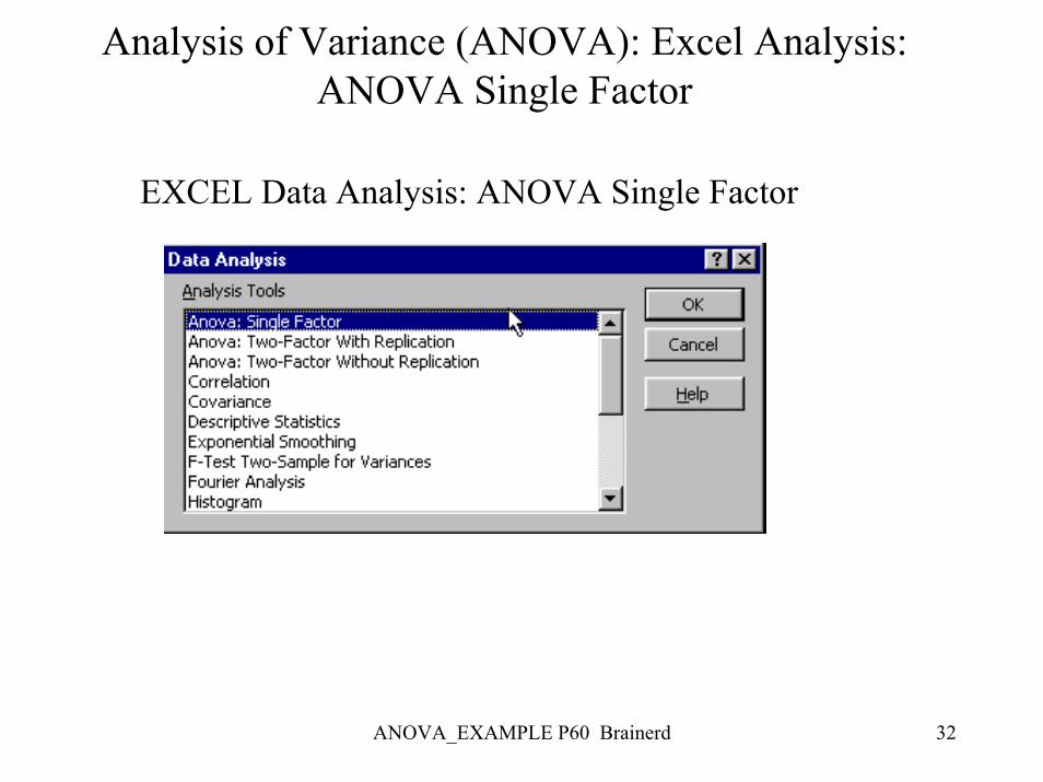
Analysis of Variance (ANOVA): Excel Analysis: ANOVA Single Factor
EXCEL Data Analysis: ANOVA Single Factor
ANOVA_EXAMPLE P60 Brainerd 33
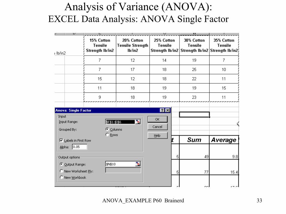
Analysis of Variance (ANOVA): EXCEL Data Analysis: ANOVA Single Factor
ANOVA_EXAMPLE P60 Brainerd 34
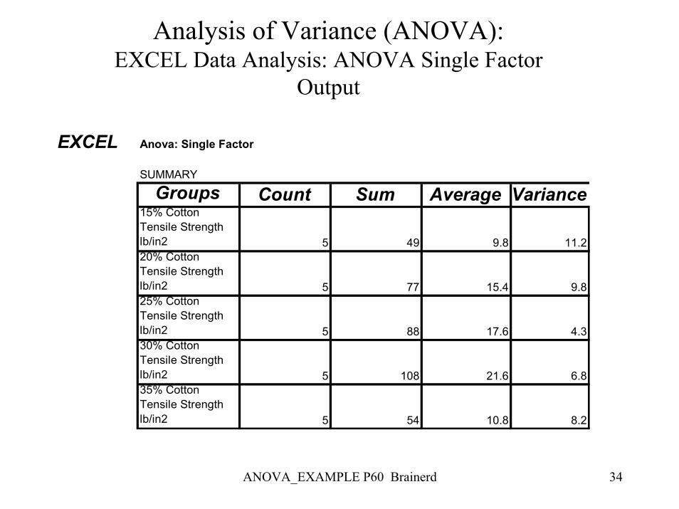
Analysis of Variance (ANOVA): EXCEL Data Analysis: ANOVA Single Factor
Output
EXCEL Anova: Single Factor
SUMMARY
Groups Count Sum Average Variance15% Cotton Tensile Strength lb/in2 5 49 9.8 11.220% Cotton Tensile Strength lb/in2 5 77 15.4 9.825% Cotton Tensile Strength lb/in2 5 88 17.6 4.330% Cotton Tensile Strength lb/in2 5 108 21.6 6.835% Cotton Tensile Strength lb/in2 5 54 10.8 8.2

ANOVA_EXAMPLE P60 Brainerd 35
Analysis of Variance (ANOVA): EXCEL Data Analysis: ANOVA Single Factor Output
ANOVASource of Variation SS df MS F P-value F critBetween Groups 475.76 4 118.94 14.75682 9.128E-06 2.866081
Within Groups 161.2 20 8.06
Total 636.96 24
MSEMSTf r=
Variation SampleWithin Variation SampleBetween
=STATTEST
)1(,1, −− JIIFα
20
20
)()(
)()(
σ
σ
=>
==
MSEEMSTE
falseHIfMSEEMSTE
trueHIf
r
r
differentisoneleastAtHH
ia
i
µµµµµ
:...: 3210 ====
P-Value: Probability of wrongly rejecting the Null
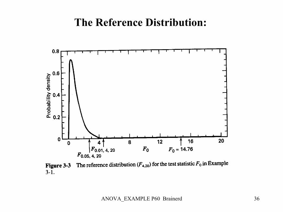
ANOVA_EXAMPLE P60 Brainerd 36
The Reference Distribution:
ANOVA_EXAMPLE P60 Brainerd 37
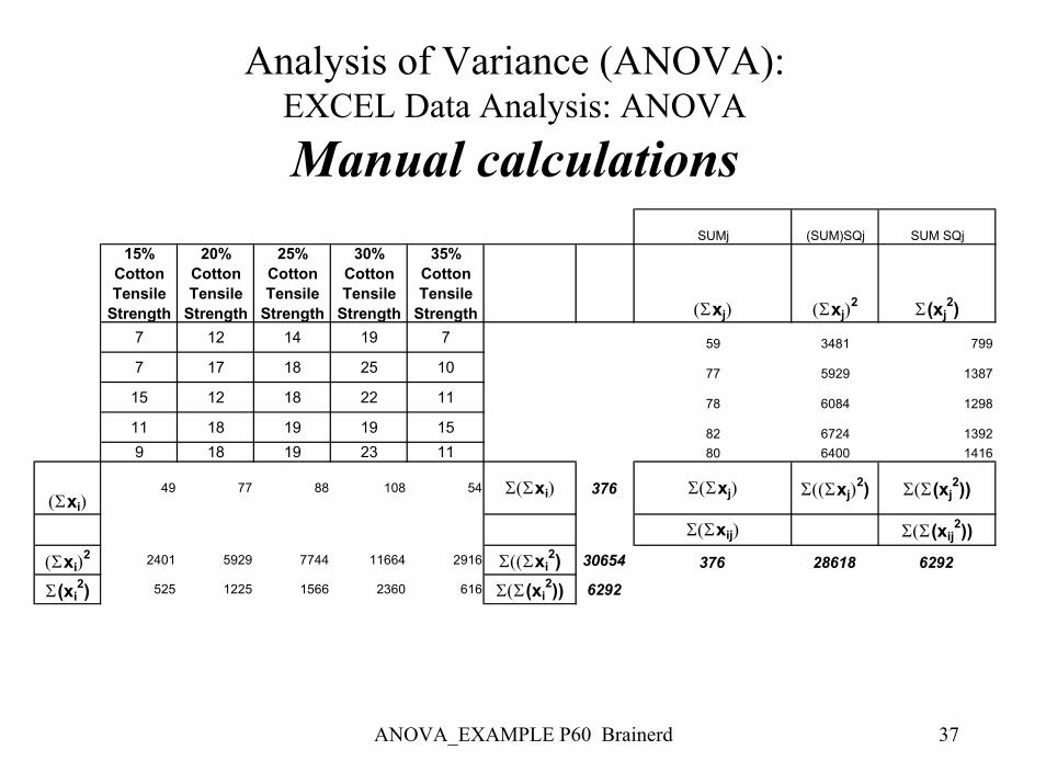
Analysis of Variance (ANOVA): EXCEL Data Analysis: ANOVA
Manual calculationsSUMj (SUM)SQj SUM SQj
15% Cotton Tensile
Strength
20% Cotton Tensile
Strength
25% Cotton Tensile
Strength
30% Cotton Tensile
Strength
35% Cotton Tensile
Strength (Σxj) (Σxj)2 Σ(xj
2)7 12 14 19 7 59 3481 799
7 17 18 25 10 77 5929 1387
15 12 18 22 11 78 6084 1298
11 18 19 19 15 82 6724 13929 18 19 23 11 80 6400 1416
(Σxi)49 77 88 108 54 Σ(Σxi) 376 Σ(Σxj) Σ((Σxj)
2) Σ(Σ(xj2))
Σ(Σxij) Σ(Σ(xij2))
(Σxi)2 2401 5929 7744 11664 2916 Σ((Σxi
2) 30654 376 28618 6292
Σ(xi2) 525 1225 1566 2360 616 Σ(Σ(xi
2)) 6292
ANOVA_EXAMPLE P60 Brainerd 38
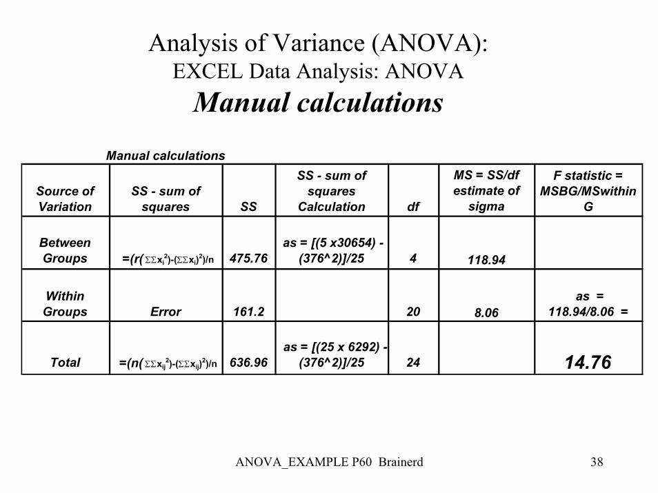
Analysis of Variance (ANOVA): EXCEL Data Analysis: ANOVA
Manual calculations
Manual calculations
Source of Variation
SS - sum of squares SS
SS - sum of squares
Calculation df
MS = SS/df estimate of
sigma
F statistic = MSBG/MSwithin
G
Between Groups =(r( ΣΣxi
2)-(ΣΣxi)2)/n 475.76 as = [(5 x30654) -
(376^2)]/25 4 118.94
Within Groups Error 161.2 20 8.06
as = 118.94/8.06 =
Total =(n( ΣΣxij2)-(ΣΣxij)2)/n 636.96
as = [(25 x 6292) -(376^2)]/25 24 14.76
ANOVA_EXAMPLE P60 Brainerd 39
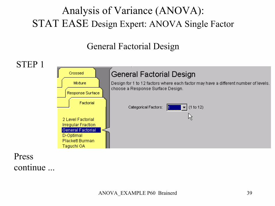
Analysis of Variance (ANOVA): STAT EASE Design Expert: ANOVA Single Factor
General Factorial Design
STEP 1
Press continue ...
ANOVA_EXAMPLE P60 Brainerd 40
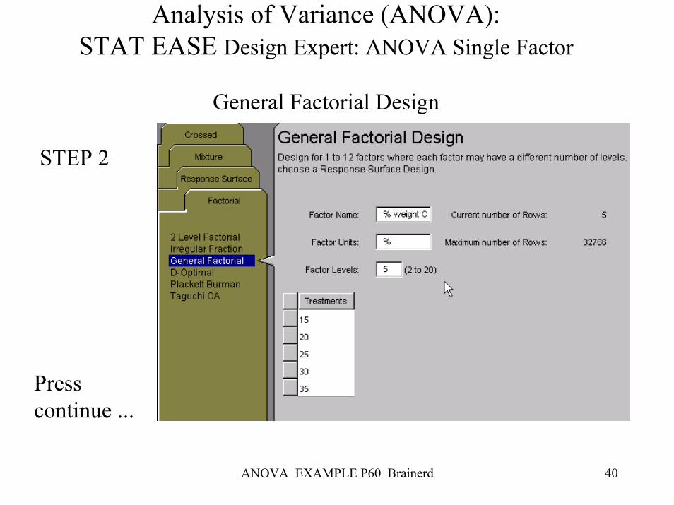
Analysis of Variance (ANOVA): STAT EASE Design Expert: ANOVA Single Factor
General Factorial Design
STEP 2
Press continue ...
ANOVA_EXAMPLE P60 Brainerd 41
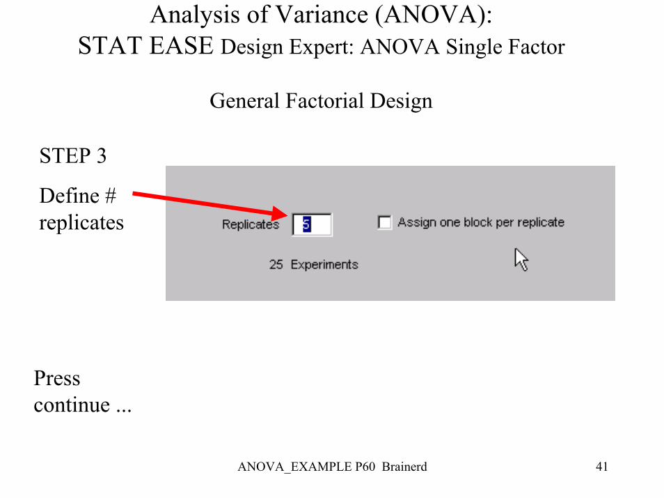
Analysis of Variance (ANOVA): STAT EASE Design Expert: ANOVA Single Factor
General Factorial Design
STEP 3
Define # replicates
Press continue ...
ANOVA_EXAMPLE P60 Brainerd 42
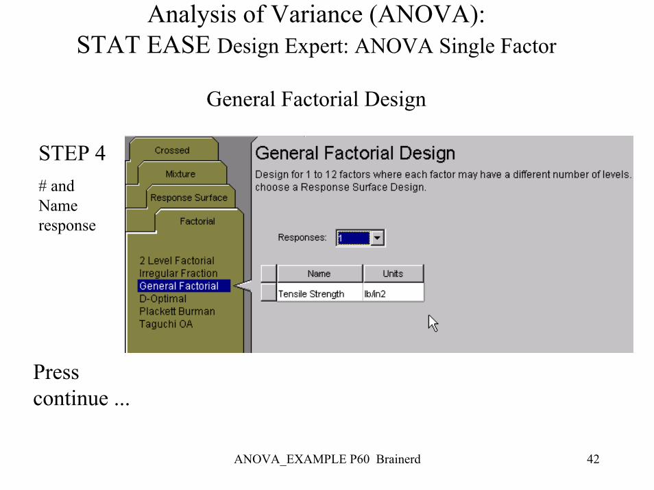
Analysis of Variance (ANOVA): STAT EASE Design Expert: ANOVA Single Factor
General Factorial Design
STEP 4# and Name response
Press continue ...
ANOVA_EXAMPLE P60 Brainerd 43
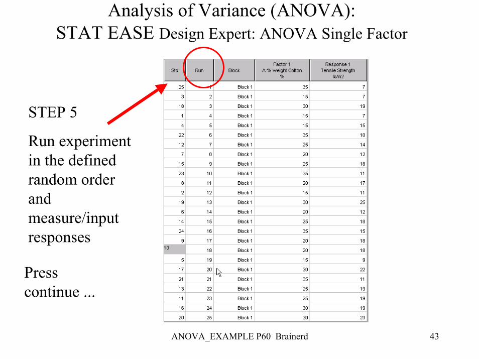
Analysis of Variance (ANOVA): STAT EASE Design Expert: ANOVA Single Factor
STEP 5
Run experiment in the defined random order and measure/input responses
Press continue ...
ANOVA_EXAMPLE P60 Brainerd 44
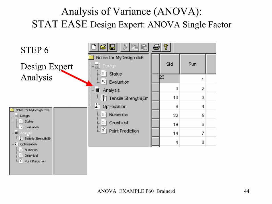
Analysis of Variance (ANOVA): STAT EASE Design Expert: ANOVA Single Factor
STEP 6
Design Expert Analysis
ANOVA_EXAMPLE P60 Brainerd 45
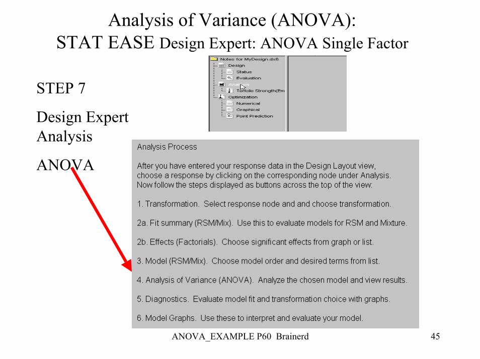
Analysis of Variance (ANOVA): STAT EASE Design Expert: ANOVA Single Factor
STEP 7
Design Expert Analysis
ANOVA
ANOVA_EXAMPLE P60 Brainerd 46
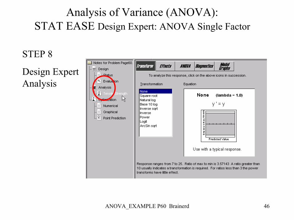
Analysis of Variance (ANOVA): STAT EASE Design Expert: ANOVA Single Factor
STEP 8
Design Expert Analysis

ANOVA_EXAMPLE P60 Brainerd 47
Analysis of Variance (ANOVA): STAT EASE Design Expert: ANOVA Single Factor
STEP 9
Design Expert Analysis
Effects
M for Model
e for error
ANOVA_EXAMPLE P60 Brainerd 48
Analysis of Variance (ANOVA): STAT EASE Design Expert: ANOVA Single Factor
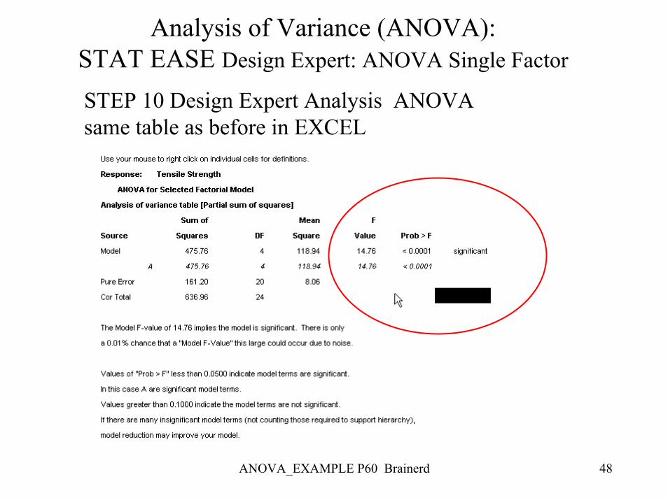
STEP 10 Design Expert Analysis ANOVA same table as before in EXCEL
ANOVA_EXAMPLE P60 Brainerd 49
Analysis of Variance (ANOVA): STAT EASE Design Expert: ANOVA Single Factor
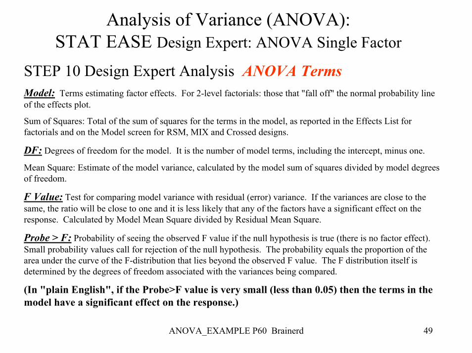
STEP 10 Design Expert Analysis ANOVA TermsModel: Terms estimating factor effects. For 2-level factorials: those that "fall off" the normal probability line of the effects plot.
Sum of Squares: Total of the sum of squares for the terms in the model, as reported in the Effects List for factorials and on the Model screen for RSM, MIX and Crossed designs.
DF: Degrees of freedom for the model. It is the number of model terms, including the intercept, minus one.
Mean Square: Estimate of the model variance, calculated by the model sum of squares divided by model degrees of freedom.
F Value: Test for comparing model variance with residual (error) variance. If the variances are close to the same, the ratio will be close to one and it is less likely that any of the factors have a significant effect on the response. Calculated by Model Mean Square divided by Residual Mean Square.
Probe > F: Probability of seeing the observed F value if the null hypothesis is true (there is no factor effect). Small probability values call for rejection of the null hypothesis. The probability equals the proportion of the area under the curve of the F-distribution that lies beyond the observed F value. The F distribution itself is determined by the degrees of freedom associated with the variances being compared.
(In "plain English", if the Probe>F value is very small (less than 0.05) then the terms in the model have a significant effect on the response.)
ANOVA_EXAMPLE P60 Brainerd 50
Analysis of Variance (ANOVA): STAT EASE Design Expert: ANOVA Single Factor
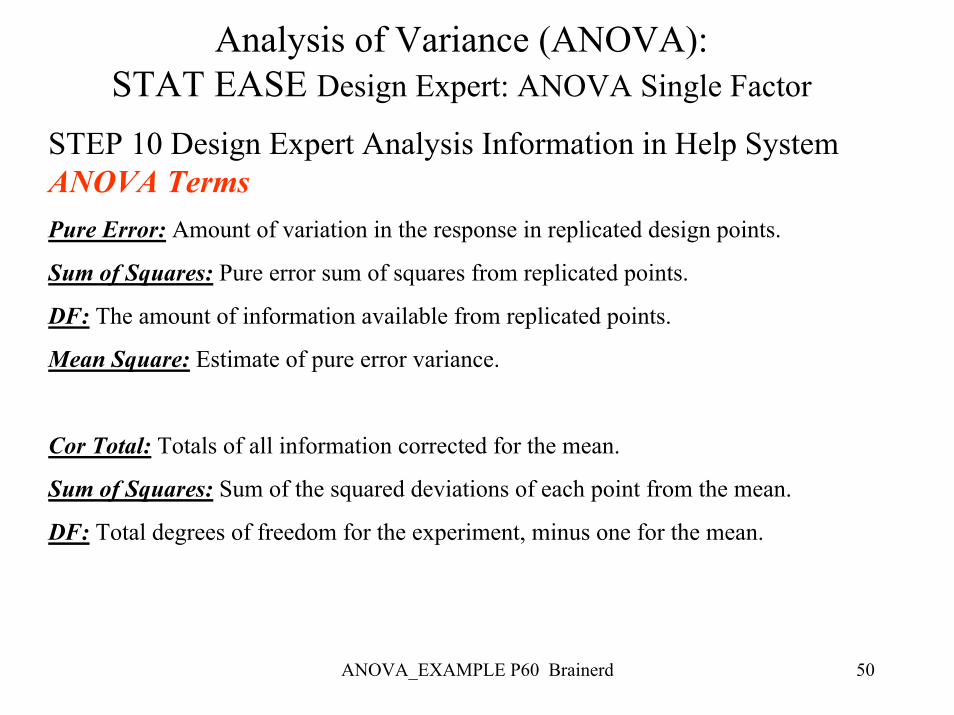
STEP 10 Design Expert Analysis Information in Help System ANOVA TermsPure Error: Amount of variation in the response in replicated design points.
Sum of Squares: Pure error sum of squares from replicated points.
DF: The amount of information available from replicated points.
Mean Square: Estimate of pure error variance.
Cor Total: Totals of all information corrected for the mean.
Sum of Squares: Sum of the squared deviations of each point from the mean.
DF: Total degrees of freedom for the experiment, minus one for the mean.
ANOVA_EXAMPLE P60 Brainerd 51
Analysis of Variance (ANOVA): STAT EASE Design Expert: ANOVA Single Factor
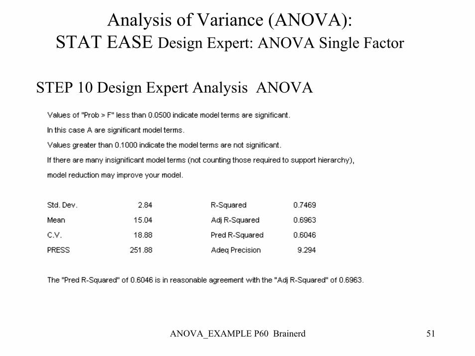
STEP 10 Design Expert Analysis ANOVA
ANOVA_EXAMPLE P60 Brainerd 52
Analysis of Variance (ANOVA): STAT EASE Design Expert: ANOVA Single Factor
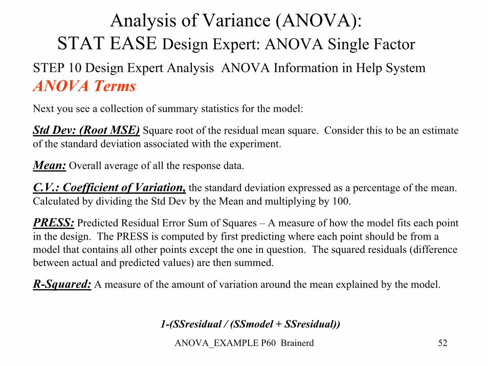
STEP 10 Design Expert Analysis ANOVA Information in Help SystemANOVA TermsNext you see a collection of summary statistics for the model:
Std Dev: (Root MSE) Square root of the residual mean square. Consider this to be an estimate of the standard deviation associated with the experiment.
Mean: Overall average of all the response data.
C.V.: Coefficient of Variation, the standard deviation expressed as a percentage of the mean. Calculated by dividing the Std Dev by the Mean and multiplying by 100.
PRESS: Predicted Residual Error Sum of Squares – A measure of how the model fits each point in the design. The PRESS is computed by first predicting where each point should be from a model that contains all other points except the one in question. The squared residuals (difference between actual and predicted values) are then summed.
R-Squared: A measure of the amount of variation around the mean explained by the model.
1-(SSresidual / (SSmodel + SSresidual))
ANOVA_EXAMPLE P60 Brainerd 53
Analysis of Variance (ANOVA): STAT EASE Design Expert: ANOVA Single Factor
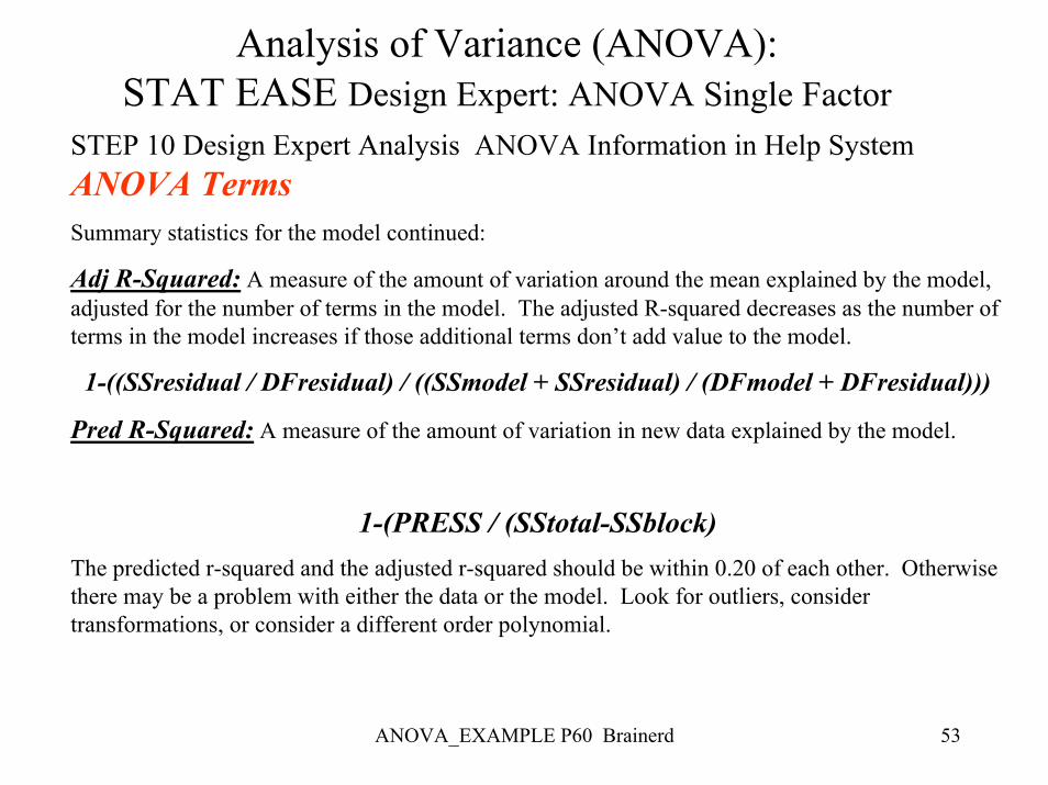
STEP 10 Design Expert Analysis ANOVA Information in Help SystemANOVA TermsSummary statistics for the model continued:
Adj R-Squared: A measure of the amount of variation around the mean explained by the model, adjusted for the number of terms in the model. The adjusted R-squared decreases as the number of terms in the model increases if those additional terms don’t add value to the model.
1-((SSresidual / DFresidual) / ((SSmodel + SSresidual) / (DFmodel + DFresidual)))
Pred R-Squared: A measure of the amount of variation in new data explained by the model.
1-(PRESS / (SStotal-SSblock)The predicted r-squared and the adjusted r-squared should be within 0.20 of each other. Otherwise there may be a problem with either the data or the model. Look for outliers, consider transformations, or consider a different order polynomial.
ANOVA_EXAMPLE P60 Brainerd 54
Analysis of Variance (ANOVA): STAT EASE Design Expert: ANOVA Single Factor
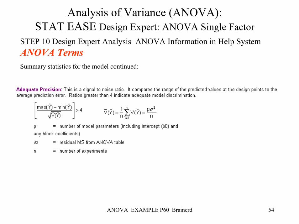
STEP 10 Design Expert Analysis ANOVA Information in Help SystemANOVA TermsSummary statistics for the model continued:
ANOVA_EXAMPLE P60 Brainerd 55
Analysis of Variance (ANOVA): STAT EASE Design Expert: ANOVA Single Factor
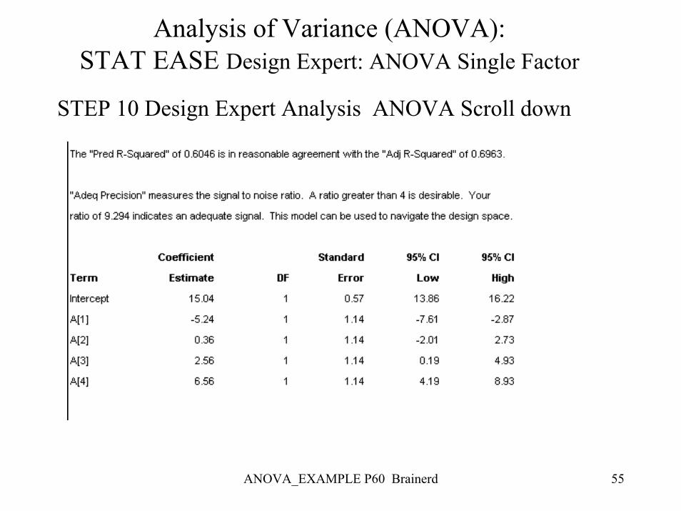
STEP 10 Design Expert Analysis ANOVA Scroll down
ANOVA_EXAMPLE P60 Brainerd 56
Analysis of Variance (ANOVA): STAT EASE Design Expert: ANOVA Single Factor
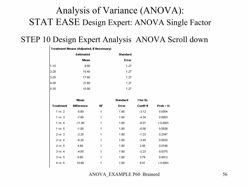
STEP 10 Design Expert Analysis ANOVA Scroll down
ANOVA_EXAMPLE P60 Brainerd 57
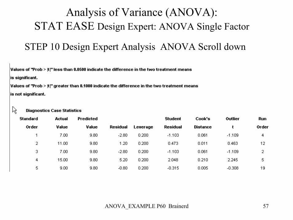
Analysis of Variance (ANOVA): STAT EASE Design Expert: ANOVA Single Factor
STEP 10 Design Expert Analysis ANOVA Scroll down
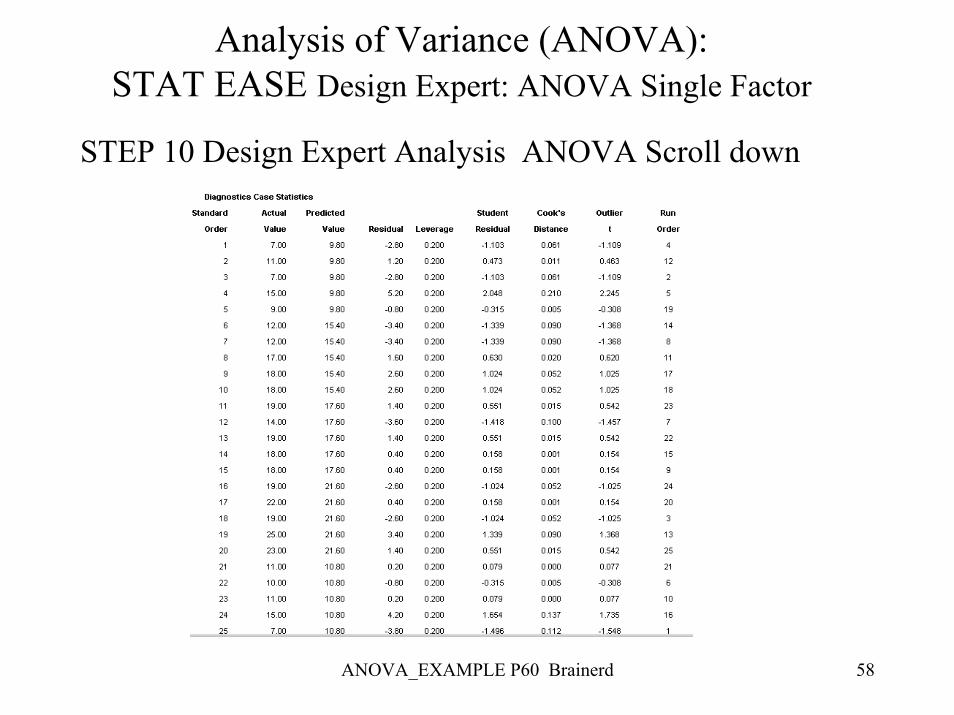
ANOVA_EXAMPLE P60 Brainerd 58
Analysis of Variance (ANOVA): STAT EASE Design Expert: ANOVA Single Factor
STEP 10 Design Expert Analysis ANOVA Scroll down
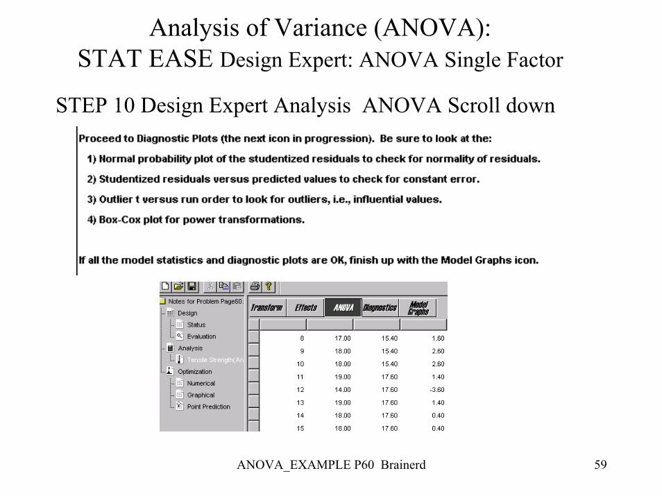
ANOVA_EXAMPLE P60 Brainerd 59
Analysis of Variance (ANOVA): STAT EASE Design Expert: ANOVA Single Factor
STEP 10 Design Expert Analysis ANOVA Scroll down
ANOVA_EXAMPLE P60 Brainerd 60
Model Adequacy Checking in the ANOVAText reference, Section 3-4, pg. 76
• Checking assumptions is important• Normality• Constant variance• Independence• Have we fit the right model?
ANOVA_EXAMPLE P60 Brainerd 61
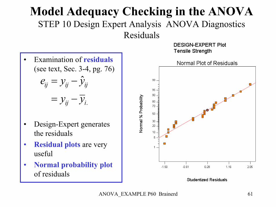
Model Adequacy Checking in the ANOVASTEP 10 Design Expert Analysis ANOVA Diagnostics
Residuals
• Examination of residuals (see text, Sec. 3-4, pg. 76)
• Design-Expert generates the residuals
• Residual plots are very useful
• Normal probability plotof residuals
.
ˆij ij ij
ij i
e y y
y y
= −
= −
ANOVA_EXAMPLE P60 Brainerd 62
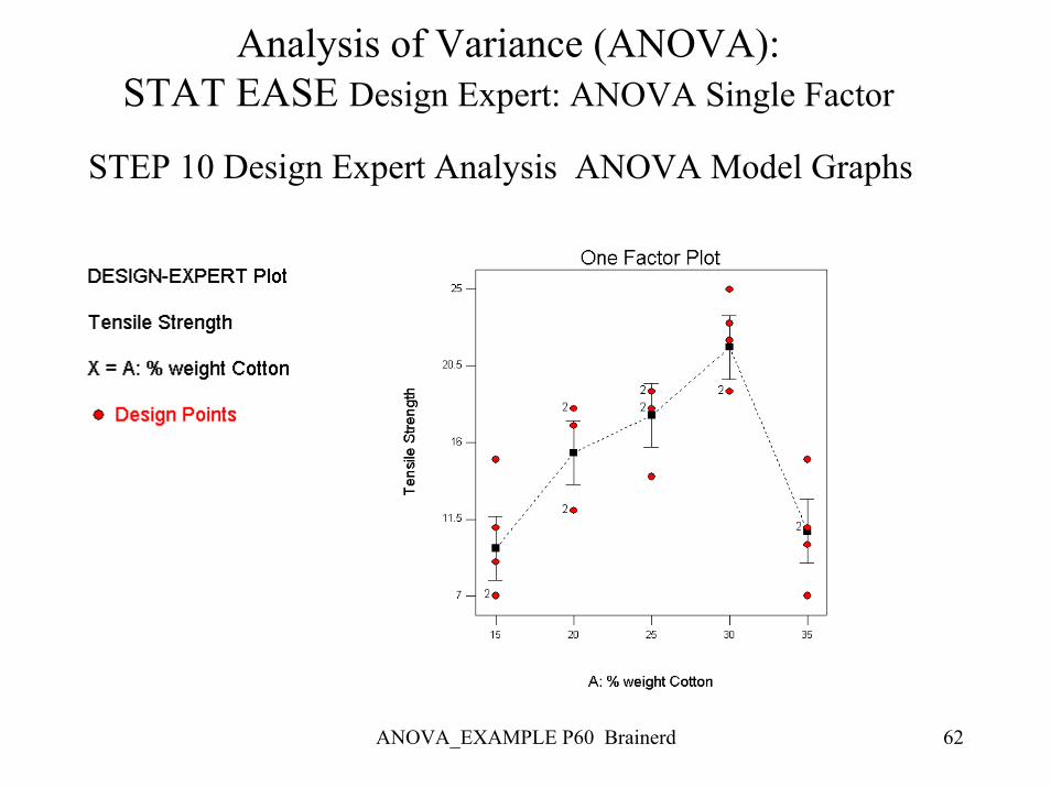
Analysis of Variance (ANOVA): STAT EASE Design Expert: ANOVA Single Factor
STEP 10 Design Expert Analysis ANOVA Model Graphs
ANOVA_EXAMPLE P60 Brainerd 63
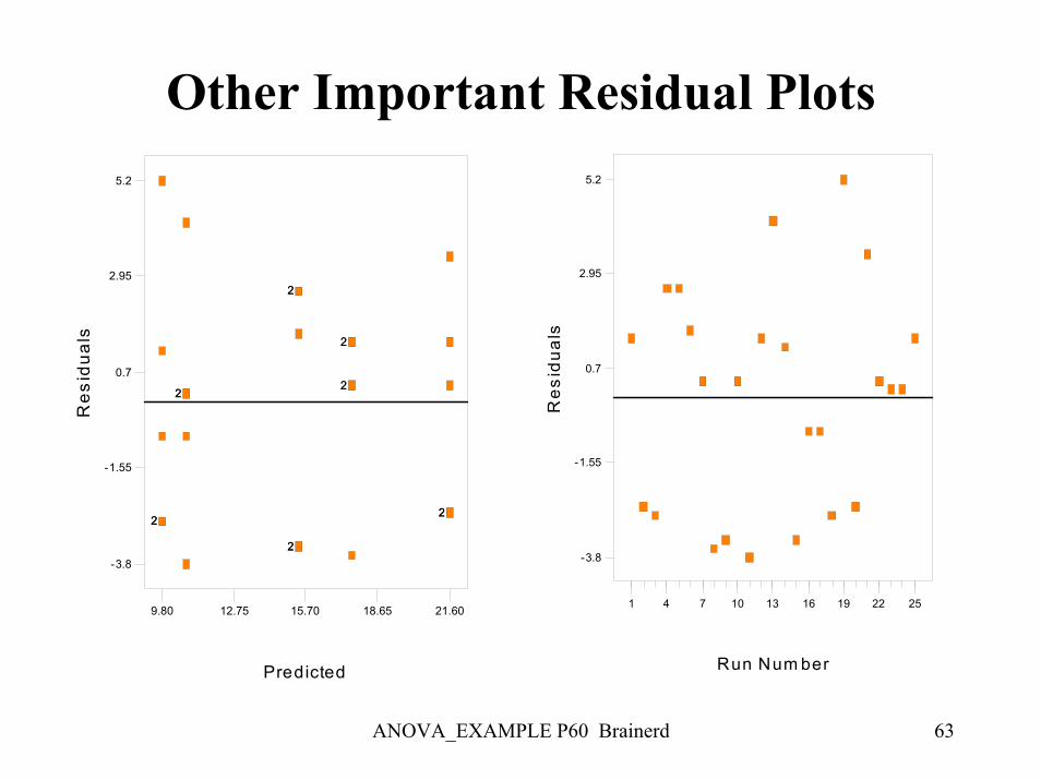
Other Important Residual Plots
Run Num ber
Res
idua
ls-3.8
-1.55
0.7
2.95
5.2
1 4 7 10 13 16 19 22 25
22
22
22
22
22
22
22
Predicted
Res
idua
ls
-3.8
-1.55
0.7
2.95
5.2
9.80 12.75 15.70 18.65 21.60
ANOVA_EXAMPLE P60 Brainerd 64
Post-ANOVA Comparison of Means• The analysis of variance tests the hypothesis of equal
treatment means• Assume that residual analysis is satisfactory• If that hypothesis is rejected, we don’t know which specific
means are different • Determining which specific means differ following an
ANOVA is called the multiple comparisons problem• There are lots of ways to do this…see text, Section 3-5, pg. 86• We will use pairwise t-tests on means…sometimes called
Fisher’s Least Significant Difference (or Fisher’s LSD) Method

ANOVA_EXAMPLE P60 Brainerd 65
Graphical Comparison of MeansText, pg. 89
ANOVA_EXAMPLE P60 Brainerd 66
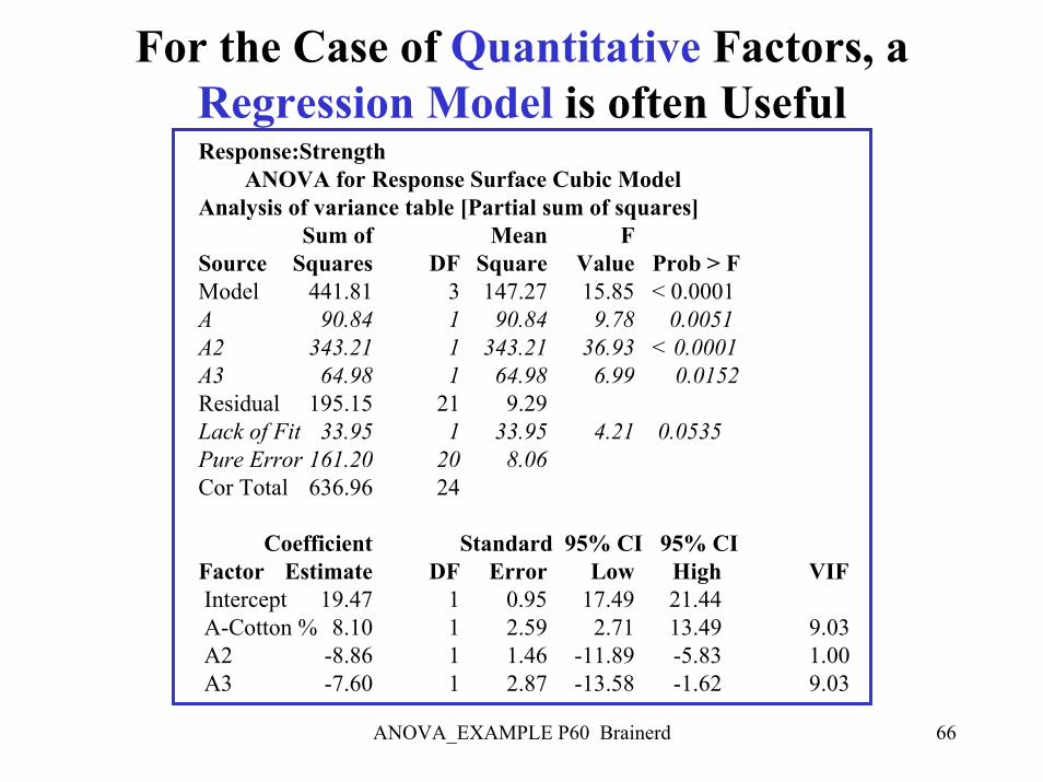
For the Case of Quantitative Factors, a Regression Model is often UsefulResponse:Strength
ANOVA for Response Surface Cubic ModelAnalysis of variance table [Partial sum of squares]
Sum of Mean FSource Squares DF Square Value Prob > FModel 441.81 3 147.27 15.85 < 0.0001A 90.84 1 90.84 9.78 0.0051A2 343.21 1 343.21 36.93 < 0.0001A3 64.98 1 64.98 6.99 0.0152Residual 195.15 21 9.29Lack of Fit 33.95 1 33.95 4.21 0.0535Pure Error 161.20 20 8.06Cor Total 636.96 24
Coefficient Standard 95% CI 95% CIFactor Estimate DF Error Low High VIFIntercept 19.47 1 0.95 17.49 21.44A-Cotton % 8.10 1 2.59 2.71 13.49 9.03A2 -8.86 1 1.46 -11.89 -5.83 1.00A3 -7.60 1 2.87 -13.58 -1.62 9.03
ANOVA_EXAMPLE P60 Brainerd 67
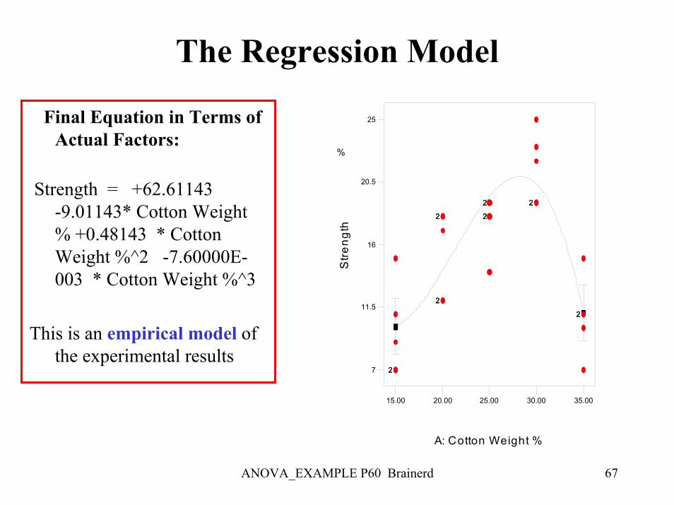
The Regression Model
Final Equation in Terms of Actual Factors:
Strength = +62.61143-9.01143* Cotton Weight % +0.48143 * Cotton Weight %^2 -7.60000E-003 * Cotton Weight %^3
This is an empirical model of the experimental results
%
15.00 20.00 25.00 30.00 35.00
7
11.5
16
20.5
25
A: Cotton Weight %
Stre
ngth
22
22
22 22
22 22
22