What Happens After A Technology Shock?∗

Lawrence J. Christiano†, Martin Eichenbaum‡and Robert Vigfusson§

August 27, 2004

Abstract

We provide empirical evidence that a positive shock to technology drives up percapita hours worked, consumption, investment, average productivity and output. Thisevidence contrasts sharply with the results reported in a large and growing literaturethat argues, on the basis of aggregate data, that per capita hours worked fall after a pos-itive technology shock. We argue that the difference in results primarily reflects specifi-cation error in the way that the literature models the low-frequency component of hoursworked.Keywords: productivity, long-run restriction, hours worked, weak instruments.

∗Christiano and Eichenbaum thank the National Science Foundation for financial assistance. The views inthis paper are solely the responsibility of the authors and should not be interpreted as reflecting the views ofthe Board of Governors of the Federal Reserve System or of any person associated with the Federal ReserveSystem. We are grateful for discussions with Susanto Basu, Lars Hansen, Valerie Ramey, and Harald Uhlig.

†Northwestern University and NBER.‡Northwestern University and NBER.§Board of Governors of the Federal Reserve System. (Email robert.j.vigfusson@frb.gov)

1 Introduction

Standard real business cycle models imply that per capita hours worked rise after a perma-nent shock to technology. Despite the a priori appeal of this prediction, there is a large andgrowing literature that argues it is inconsistent with the data. This literature uses reducedform time series methods in conjunction with minimal identifying assumptions that holdacross large classes of models to estimate the actual effects of a technology shock. The re-sults reported in this literature are important because they call into question basic propertiesof many structural business cycle models.Consider, for example, the widely cited paper by Gali (1999). His basic identifying

assumption is that innovations to technology are the only shocks that have an effect onthe long run level of labor productivity. Gali (1999) reports that hours worked fall after apositive technology shock. The fall is so long and protracted that, according to his estimates,technology shocks are a source of negative correlation between output and hours worked.Because hours worked are in fact strongly procyclical, Gali concludes that some other shockor shocks must play the predominant role in business cycles with technology shocks at bestplaying only a minor role. Moreover, he argues that standard real business cycle modelsshed little light on whatever small role technology shocks do play because they imply thathours worked rise after a positive technology shock. In effect, real business cycle models aredoubly damned: they address things that are unimportant, and they do it badly at that.Other recent papers reach conclusions that complement Gali’s in various ways (see, e.g.,Shea (1998), Basu, Kimball and Fernald (1999), and Francis and Ramey (2003)). In view ofthe important role attributed to technology shocks in business cycle analyses of the past twodecades, Francis and Ramey perhaps do not overstate too much when they say (p.2) thatGali’s argument is a ‘...potential paradigm shifter’.Not surprisingly, the result that hours worked fall after a positive technology shock has

attracted a great deal of attention. Indeed, there is a growing literature aimed at constructinggeneral equilibrium business cycle models that can account for this result. Gali (1999) andothers have argued that the most natural explanation is based on sticky prices. Others, likeFrancis and Ramey (2003) and Vigfusson (2004), argue that this finding is consistent withreal business cycle models modified to allow for richer sets of preferences and technology,such as habit formation and investment adjustment costs.1

We do not build a model that can account for the result that hours fall after a technologyshock. Instead, we challenge the result itself. Using the same identifying assumption as Gali(1999), Gali, Lopez-Salido, and Valles (2002), and Francis and Ramey (2003), we find thata positive technology shock drives hours worked up, not down.2 In addition, it leads to arise in output, average productivity, investment, and consumption. That is, we find that apermanent shock to technology has qualitative consequences that a student of real businesscycles would anticipate.3 At the same time, we find that permanent technology shocks play

1Other models that can account for the Gali (1999) finding are contained in Christiano and Todd (1996)and Boldrin, Christiano and Fisher (2001).

2Chang and Hong (2003) obtain similar results using disaggregated data.3That the consequences of a technology shock resemble those in a real business cycle model may well

reflect that the actual economy has various nominal frictions, and monetary policy has successfully mitigatedthose frictions. See Altig, Christiano, Eichenbaum and Linde (2002) for empirical evidence in favor of this

1

a very small role in business cycle fluctuations. Instead, they are quantitatively importantat frequencies of the data that a student of traditional growth models might anticipate.Since we make the same fundamental identification assumption as Gali (1999), Gali,

Lopez-Salido, and Valles (2002) and Francis and Ramey (2003), the key questions is: Whataccounts for the difference in our findings? By construction, the difference must be dueto different maintained assumptions. As it turns out, a key culprit is how we treat hoursworked. If we assume, as do Francis and Ramey, that per capita hours worked is a differencestationary process and work with the growth rate of hours (the difference specification), thenwe too find that hours worked falls after a positive technology shock. But if we assume thatper capita hours worked is a stationary process and work with the level of hours worked (thelevel specification), then we find the opposite: hours worked rise after a positive technologyshock.So we have two answers to the question, ‘what happens to hours worked after a positive

technology shock?’ Each answer is based on a different statistical model, depending on thespecification of hours worked. To judge between the competing specifications, we use classicalstatistical methods as well as encompassing methods that quantify the relative plausibilityof the two specifications.Our classical statistical analysis focuses on the question of whether per capita hours

have a unit root. As is well known, standard univariate unit root tests like the AugmentedDickey Fuller (ADF) test have very poor power properties relative to the alternative thatthe series in question is a persistent stationary stochastic process. However, Hansen (1995)and Elliott and Jansson (2003) argue that large power gains can be achieved by includingcorrelated stationary covariates in the regression equation underlying the ADF test statistic.Motivated by these results, we test the null hypothesis that per capita hours worked has aunit root using a version of Hansen’s covariate augmented Dicky-Fuller (CADF) test. Wefind strong evidence against this null hypothesis. Given the importance of this result for ourargument, we conduct our own Monte Carlo study to document that the CADF test hasmuch more power than the ADF test (see Appendix B).To assess the relative plausibility of the level and difference specifications, we adopt an

encompassing approach. Specifically, we ask the question, ‘which specification has an easiertime explaining the observation that hours worked falls under the difference specificationand rises under the level specification?’ Consistent with our classical analysis, this criterionalso leads us to prefer the level specification.We now discuss the results that lead to this conclusion. First, the level specification

encompasses the difference specification. We show this by calculating what an analyst whoadopts the difference specification would find if our estimated level specification were true.For reasons discussed below, by differencing hours worked this analyst commits a specifi-cation error. We find that such an analyst would, on average, infer that hours worked fallafter a positive technology shock even though they rise in the true data-generating process.Indeed the extent of this fall is very close to the actual decline in hours worked implied bythe estimated difference specification. The level specification also easily encompasses theimpulse responses of the other relevant variables.Second, the difference specification does not encompass the level specification. We calcu-

interpretation.

2

late what an analyst who adopts the level specification would find if our estimated differencespecification were true. The mean prediction is that hours fall after a technology shock. So,focusing on means alone, the difference specification cannot account for the actual estimatesassociated with the level representation. However, the difference specification predicts thatthe impulse responses based on the level representation vary a great deal across repeatedsamples. This uncertainty is so great that the difference specification can account for thelevel results as an artifact of sampling uncertainty. This result, however, is a Pyrrhic victoryfor the difference specification. The prediction of large sampling uncertainty stems from thedifference specification’s prediction that an econometrician working with the level specifica-tion encounters a version of the weak instrument problem analyzed in the literature (see, forexample, Staiger and Stock, 1997). A standard weak instrument test applied to the datafinds little evidence of such a problem. This result is not surprising because, in our context,the weak instrument test is identical to Hansen’s CADF test for a unit root in per capitahours work.To quantify the relative plausibility of the level and difference specifications, we compute

the type of posterior odds ratio considered in Christiano and Ljungqvist (1988). The basicidea is that the more plausible of the two specifications is the one that has the easiesttime explaining the facts: (i) the level specification implies that hours worked rises after atechnology shock, (ii) the difference specification implies that hours worked falls, and (iii)the outcome of the weak instruments test. Focusing only on facts (i) and (ii), we find thatthe odds are roughly 2 to 1 in favor of the level specification over the difference specification.However, once (iii) is incorporated into the analysis, we find that the odds overwhelminglyfavor the level specification, by at least 58 to 1.Finally, we assess the robustness of our results against alternative ways of modeling low

frequency movements in the variables entering our analysis. The basic issue is that in oursample period per capita hours worked exhibit a U shaped pattern while other variableslike inflation and the federal funds rate display hump-shaped patterns. Accordingly wetest for the presence of a quadratic trend in these variables. After correcting for the smallsample distribution of the relevant t statistics, we do not reject the null hypothesis that thecoefficients on the time-squared terms in per capita hours, inflation and the federal fund areequal to zero.Although supportive of our level specification, this result may just reflect the possibility

that our tests suffer from low power. To this end, we redid our analysis with three types ofquadratic trend specifications to assess the robustness of inference. In case (i) we removequadratic trends from all the variables before estimating the VAR. In case (ii) we removequadratic trends from per capita hours worked, inflation and the federal funds rate beforeestimating the VAR. Finally, in case (iii) we remove a quadratic trend only from per capitahours worked before estimating the VAR. As it turns out, the only case in which inferenceis not robust is case (iii), where hours worked fall in a persistent way after a positive shockto technology. The problem with this case is that it treats hours worked differently fromthe other variables in terms of allowing for a quadratic trend. We see no rationale forthis asymmetry. Consequently, we attach little importance to case (iii). To quantify therelative plausibility of this case, we use a posterior odds ratio like the one discussed above.Our analysis focuses on the models’ ability to account for (a) the t statistics associated withstandard classical tests for quadratic trends in per capita hours worked, inflation and the

3

federal funds rate, and (b) the sign of the response of per capita hours worked to a technologyshock in the different cases. We find that the preponderance of the evidence strongly favorsall of the alternatives to case (iii): the odds in favor of case (i), (ii) and the level specificationare 20, 8, and 4 to one, respectively. We conclude that inference about the response of percapita hours is robust in all but the least plausible case.The remainder of this paper is organized as follows. Section 2 discusses our strategy for

identifying the effects of a permanent shock to technology. Section 3 presents our empiricalresults for the level and difference specifications. In Section 4 we discuss the results of classicaltests for assessing the different specifications. Section 5 discusses our encompassing methodand reports our results. Section 6 explores the robustness of inference to the possible presenceof deterministic trends. In addition, we examine the subsample stability of our time seriesmodel. In Section 7 we report our findings regarding the overall importance of technologyshocks in cyclical fluctuations. Section 8 contains concluding remarks.

2 Identifying the Effects of a Permanent Technology

Shock

In this section, we discuss our strategy for identifying the effects of permanent shocks totechnology. We follow Gali (1999), Gali, Lopez-Salido, and Valles (2002) and Francis andRamey (2003) and adopt the identifying assumption that the only type of shock that affectsthe long-run level of average labor productivity is a permanent shock to technology. Thisassumption is satisfied by a large class of standard business cycle models. See, for example,the real business cycle models in Christiano (1988), King, Plosser, Stock and Watson (1991)and Christiano and Eichenbaum (1992) which assume that technology shocks are a differencestationary process.4

As discussed below, we use reduced form time series methods in conjunction with ouridentifying assumption to estimate the effects of a permanent shock to technology. An ad-vantage of this approach is that we do not need to make all the usual assumptions required toconstruct Solow-residual based measures of technology shocks. Examples of these assump-tions include corrections for labor hoarding, capital utilization, and time-varying markups.5

Of course there exist models that do not satisfy our identifying assumption. For example, theassumption is not true in an endogenous growth model where all shocks affect productivityin the long run. Nor is it true in an otherwise standard model when there are permanentshocks to the tax rate on capital income.6 These caveats notwithstanding, we proceed as inthe literature.

4If these models were modified to incorporate permanent shocks to agents’ preferences for leisure or togovernment spending, these shocks would have no long run impact on labor productivity, because laborproductivity is determined by the discount rate and the underlying growth rate of technology.

5See Basu, Fernald and Kimball (1999) for an interesting application of this alternative approach. Vig-fusson (2004) combines these two approaches by using a constructed technology series in place of laborproductivity in a VAR with a long-run identification assumption.

6Uhlig (2004) and Gali and Rabanal (2004) argue on empirical grounds that the shocks estimated using theidentifying assumptions imposed in this papers and the relevant literature do not correspond to permanentshocks to the tax rate on capital income.

4

We estimate the dynamic effects of a technology shock using the method proposed inShapiro and Watson (1988). The starting point of the approach is the relationship:

∆ft = µ+ β(L)∆ft−1 + α(L)Xt + εzt . (1)

Here ft denotes the log of average labor productivity and α(L), β(L) are polynomials oforder q and q− 1 in the lag operator, L, respectively. Also, ∆ is the first difference operatorand we assume that ∆ft is covariance stationary. The white noise random variable, εzt ,is the innovation to technology. Suppose that the response of Xt to an innovation in somenon-technology shock, εt, is characterized byXt = γ(L)εt, where γ(L) is a polynomial in non-negative powers of L. We assume that each element of γ(1) is non-zero. The assumption thatnon-technology shocks have no impact on ft in the long run implies the following restrictionon α(L) :

α(L) = α(L)(1− L), (2)

where α(L) is a polynomial of order q − 1 in the lag operator. To see this, note first thatthe only way non-technology shocks can have an impact on ft is by their effect on Xt, whilethe long-run impact of a shock to εt on ft is given by:

α(1)γ(1)

1− β(1).

The assumption that ∆ft is covariance stationary guarantees |1− β(1)| <∞. This assump-tion, together with our assumption on γ(L), implies that for the long-run impact of εt on ftto be zero it must be that α(1) = 0. This in turn is equivalent to (2).Substituting (2) into (1) yields the relationship:

∆ft = µ+ β(L)∆ft−1 + α(L)∆Xt + εzt . (3)

We obtain an estimate of εzt by using (3) in conjunction with estimates of µ, β(L) and α(L).If one of the shocks driving Xt is εzt , then Xt and εzt will be correlated. So, we cannotestimate the parameters in β(L) and α(L) by ordinary least squares (OLS). Instead, weapply the standard instrumental variables strategy used in the literature. In particular, weuse as instruments a constant, ∆ft−s and Xt−s, s = 1, 2, ...,q.Given an estimate of the shocks in (3), we obtain an estimate of the dynamic response of ft

and Xt to εzt as follows. We begin by estimating the following q

th order vector autoregression(VAR):

Yt = α+B(L)Yt−1 + ut, Eutu0t = V, (4)

where

Yt =

µ∆ftXt

¶,

and ut is the one-step-ahead forecast error in Yt. Also, V is a positive definite matrix. Theparameters in this VAR, including V, can be estimated by OLS applied to each equation.In practice, we set q = 4. The fundamental economic shocks, et, are related to ut by thefollowing relation:

ut = Cet, Eete0t = I.

5

Without loss of generality, we suppose that εzt is the first element of et. To compute thedynamic response of the variables in Yt to ε

zt , we require the first column of C. We obtain this

column by regressing ut on εzt by ordinary least squares. Finally, we simulate the dynamicresponse of Yt to εzt . For each lag in this response function, we computed the centered 95percent Bayesian confidence interval using the approach for just-identified systems discussedin Doan (1992).7

3 Empirical Results

In this section we present our benchmark empirical results. The first subsection reportsresults based on a simple bivariate VAR. In the level specification of this VAR, ft is the logof business labor productivity and Xt (the second element in Yt) is the log level of hoursworked in the business sector divided by a measure of the population, ht.

8 In the differencespecification, Xt is the growth rate of hours worked, ∆ht. To assess the robustness of ourresults to alternative measures of productivity and hours worked, we re-did our analysisusing alternative measures of productivity and hours worked. In all cases our qualitativefindings were the same.9 In section (6.1) we consider the sensitivity of our analysis to thepossibility that ht is stationary about a quadratic trend.In the second subsection we extend our analysis to allow for a richer set of variables. We

do so for two reasons. First, the responses of these other variables are interesting in theirown right. Second, there is no a priori reason to expect that the answers generated fromsmall bivariate systems will survive in larger dimensional systems. If variables other thanhours worked belong in the basic relationship governing the growth rate of productivity, andthese are omitted from (1), then simple bivariate analysis will not generally yield consistentestimates of innovations to technology.Our extended system allows for four additional macroeconomic variables: the federal

funds rate, the rate of inflation, the log of the ratio of nominal consumption expenditures tonominal GDP, and the log of the ratio of nominal investment expenditures to nominal GDP.10

The last two variables correspond to the ratio of real investment and consumption, measuredin units of output, to total real output. Standard models, including those that allow for

7This approach requires drawing B(L) and V repeatedly from their posterior distributions. Our resultsare based on 2, 500 draws.

8Our data were taken from the DRI Economics database. The mnemonic for business labor productivity isLBOUT. The mnemonic for business hours worked is LBMN. The business hours worked data were convertedto per capita terms using a measure of the civilian population over the age of 16 (mnemonic, P16).

9The alternative measures of productivity and hours which we considered were (i) real GDP divided bytotal business hours, business hours worked divided by civilian population over the age of 16), (ii) real GDPdivided by non-farm business hours worked, non-farm business hours worked divided by civilian populationover the age of 16, (iii) non - farm business output divided by non farm business hours worked, non farmbusiness hours worked divided by civilian population over the age of 16.10Our measures of the growth rate of labor productivity and hours worked are the same as in the bivariate

system. We measured inflation using the growth rate of the GDP deflator, measured as the ratio of nominaloutput to real output (GDP/GDPQ). Consumption is measured as consumption on nondurables and servicesand government expenditures: (GCN+GCS+GGE). Investment is measured as expenditures on consumerdurables and private investment: (GCD+GPI). The federal funds series corresponds to FYFF. All mnemonicsrefer to DRI’s BASIC economics database.

6

investment-specific technical change, imply these two variables are covariance stationary.11

Data on our six variables are displayed in Figure 1.We choose to work with per capita hours worked, rather than total hours worked, because

this is the object that appears in most general equilibrium business cycle models. Thereare two additional reasons for this choice. First, for our short sample period, classicalstatistical tests yield strong evidence against the difference stationary specification of logtotal hours worked.12 Because the short sample plays an important role in our analysis,we are uncomfortable adopting the difference stationary specification. Second, suppose weassume, as in Gali (1999), that the log of hours is stationary about a linear trend. We findthis specification unappealing because it implies that permanent shocks, originating fromdemographic factors, to total hours and total output are ruled out. By working with percapita hours, we do not exclude the possibility that demographic shocks have permanenteffects on total hours worked and total output. In sum, it is clear that total hours workedare not a stationary process. But we are uncomfortable modeling this non-stationarity byeither a simple unit root or a linear trend. Rather than adopt a non-standard model of thelow frequency component of total hours worked, we focus on per capita hours worked.

3.1 Bivariate Results

In this subsection we report results based on a bivariate VAR of labor productivity growthand hours worked. We consider two sample periods. The longest period for which data areavailable on the variables in our VAR is 1948Q1-2001Q4. We refer to this as the long sample.The start of this sample period coincides with the one in Francis and Ramey (2003) and Gali(1999). Francis and Ramey (2003) and Gali, Lopez-Salido, and Valles (2002) work, as wedo, with per capita hours worked, while Gali (1999) works with total hours worked. Sincemuch of the business cycle literature works with post-1959 data, we also consider a secondsample period given by 1959Q1-2001Q4. We refer to this as the short sample.We now turn to our results. Panel A of Figure 2 displays the response of log output and

log hours to a positive technology shock, based on the long sample. A number of interestingresults emerge here. First, the impact effect of the shock on output and hours is positive(1.17 percent and 0.34 percent, respectively) after which both rise in a hump shaped pattern.The responses of output are statistically significantly different from zero over the 20 quartersdisplayed. Second, in the long run, output rises by 1.33 percent. By construction the long

11See for example Altig, Christiano, Eichenbaum and Linde (2002). This paper posits that investmentspecific technical change is trend stationary. See also Fisher (2003), which assumes investment specifictechnical change is difference stationary. Both frameworks imply that the consumption and investmentratios discussed in the text are stationary.12Specifically, we regressed the growth rate of total hours worked on a constant, time, the lag level of log

total hours worked and four lags of the growth rate of total hours worked and 4 lags of productivity growth.We then computed the F statistic for the null hypothesis that the coefficient on the lag level of log total hoursworked and the coefficient on time are jointly zero. This amounts to a test of the null hypothesis that logtotal hours worked is difference stationary, against the alternative that it is stationary about a linear trend.We reject this null hypothesis at the 1 percent significance value. We used the tabulated critical values in‘Case 4’, Table B.7, of Hamilton (1994, p. 764). To check these, we also computed bootstrap critical valuesby simulating a bivariate, 4-lag VAR fit to data on the growth rate of productivity and the growth rate oftotal hours. The calculations were performed using the short and long sample periods.

7

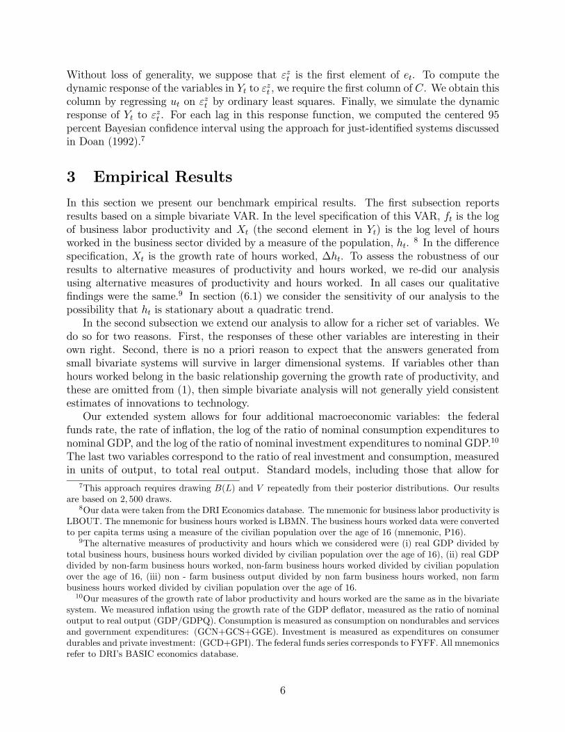
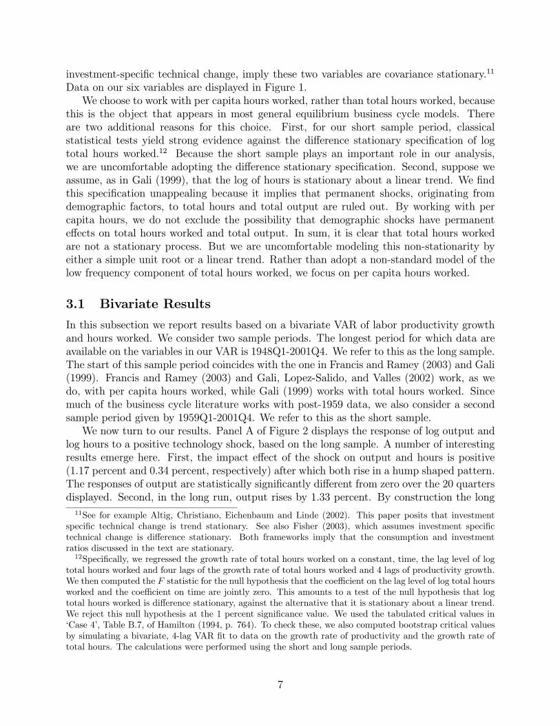
run effect on hours worked is zero. The response of hours worked is statistically significantduring the time period between two and ten quarters after the impact of the shock. Third,since output rises by more than hours does, labor productivity also rises in response to apositive technology shock.Panel B of Figure 2 displays the analogous results for the short sample period. As

before, the impact effect of the shock on output and hours is positive (0.94 and 0.14 percent,respectively), after which both rise in a hump-shaped pattern. The long run impact of theshock is to raise output by 0.96 percent. Again, average productivity rises in response to theshock and there is no long run effect on hours worked. So regardless of which sample periodwe use, the same picture emerges: a permanent shock to technology drives hours, outputand average productivity up.The previous results stand in sharp contrast to the literature according to which hours

worked fall after a positive technology shock. The difference cannot be attributed to ouridentifying assumptions or the data that we use. We can reproduce the bivariate-basedresults in the literature if we assume that Xt in (1) and (3) corresponds to the growth rateof hours worked rather than the level of hours worked. The two panels in Figure 3 displaythe analogous results to those in Figure 2 with this change in the definition of Xt.According to the point estimates displayed in Panels A and B of Figure 3, a positive shock

to technology induces a rise in output, but a persistent decline in hours worked.13 Confidenceintervals are clearly very large. Still, the initial decline in hours worked is statisticallysignificant. This result is consistent with the bivariate analysis in Gali (1999) and Francisand Ramey (2003).

3.2 Moving Beyond Bivariate Systems

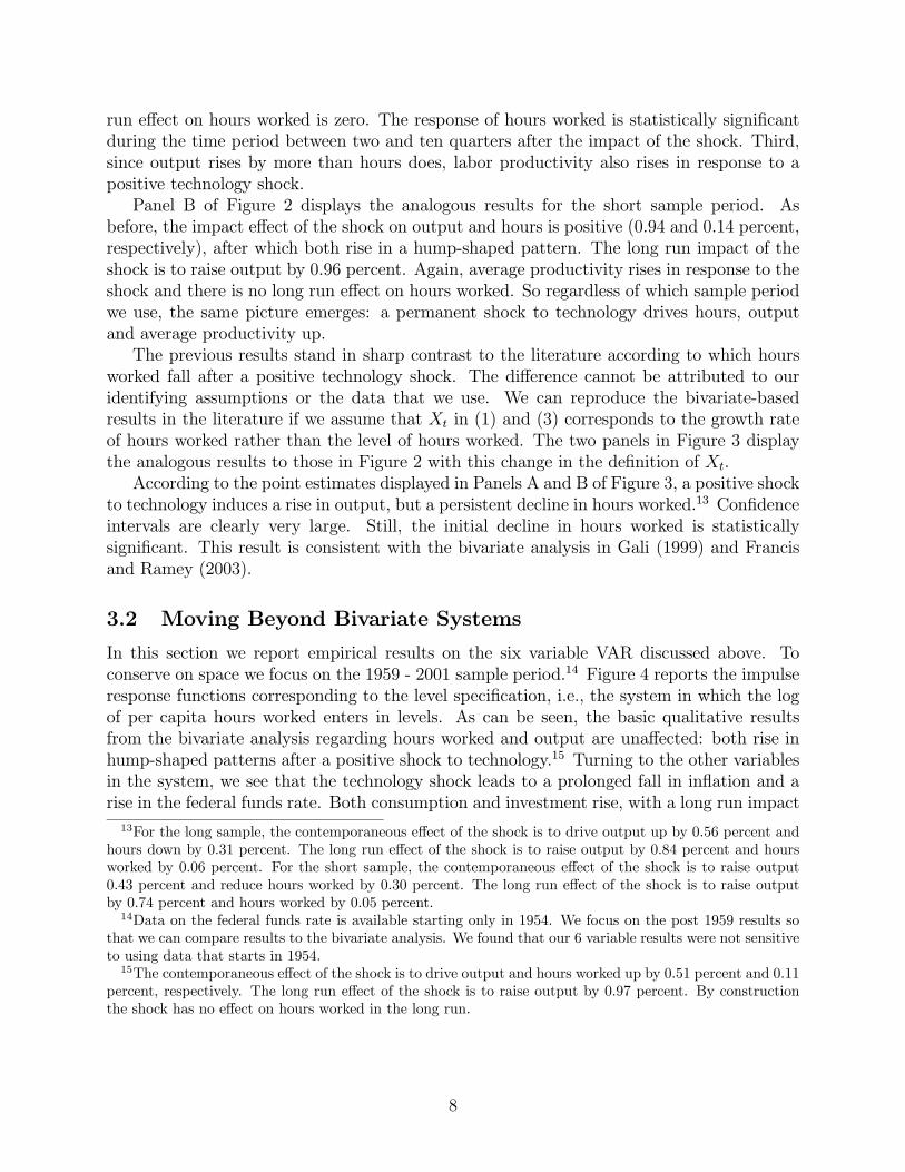
In this section we report empirical results on the six variable VAR discussed above. Toconserve on space we focus on the 1959 - 2001 sample period.14 Figure 4 reports the impulseresponse functions corresponding to the level specification, i.e., the system in which the logof per capita hours worked enters in levels. As can be seen, the basic qualitative resultsfrom the bivariate analysis regarding hours worked and output are unaffected: both rise inhump-shaped patterns after a positive shock to technology.15 Turning to the other variablesin the system, we see that the technology shock leads to a prolonged fall in inflation and arise in the federal funds rate. Both consumption and investment rise, with a long run impact

13For the long sample, the contemporaneous effect of the shock is to drive output up by 0.56 percent andhours down by 0.31 percent. The long run effect of the shock is to raise output by 0.84 percent and hoursworked by 0.06 percent. For the short sample, the contemporaneous effect of the shock is to raise output0.43 percent and reduce hours worked by 0.30 percent. The long run effect of the shock is to raise outputby 0.74 percent and hours worked by 0.05 percent.14Data on the federal funds rate is available starting only in 1954. We focus on the post 1959 results so

that we can compare results to the bivariate analysis. We found that our 6 variable results were not sensitiveto using data that starts in 1954.15The contemporaneous effect of the shock is to drive output and hours worked up by 0.51 percent and 0.11

percent, respectively. The long run effect of the shock is to raise output by 0.97 percent. By constructionthe shock has no effect on hours worked in the long run.

8

that is, by construction, equal to the long run rise in output.16

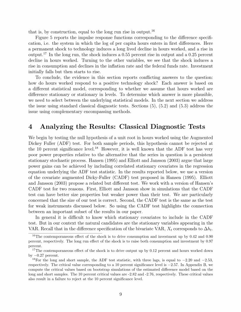
Figure 5 reports the impulse response functions corresponding to the difference specifi-cation, i.e. the system in which the log of per capita hours enters in first differences. Herea permanent shock to technology induces a long lived decline in hours worked, and a rise inoutput.17 In the long run, the shock induces a 0.55 percent rise in output and a 0.25 percentdecline in hours worked. Turning to the other variables, we see that the shock induces arise in consumption and declines in the inflation rate and the federal funds rate. Investmentinitially falls but then starts to rise.To conclude, the evidence in this section reports conflicting answers to the question:

how do hours worked respond to a positive technology shock? Each answer is based ona different statistical model, corresponding to whether we assume that hours worked aredifference stationary or stationary in levels. To determine which answer is more plausible,we need to select between the underlying statistical models. In the next section we addressthe issue using standard classical diagnostic tests. Sections (5), (5.2) and (5.3) address theissue using complementary encompassing methods.

4 Analyzing the Results: Classical Diagnostic Tests

We begin by testing the null hypothesis of a unit root in hours worked using the AugmentedDickey Fuller (ADF) test. For both sample periods, this hypothesis cannot be rejected atthe 10 percent significance level.18 However, it is well known that the ADF test has verypoor power properties relative to the alternative that the series in question is a persistentstationary stochastic process. Hansen (1995) and Elliott and Jansson (2003) argue that largepower gains can be achieved by including correlated stationary covariates in the regressionequation underlying the ADF test statistic. In the results reported below, we use a versionof the covariate augmented Dicky-Fuller (CADF) test proposed in Hansen (1995). Elliottand Jansson (2003) propose a related but different test. We work with a version of Hansen’sCADF test for two reasons. First, Elliott and Jansson show in simulations that the CADFtest can have better size properties but weaker power than their test. We are particularlyconcerned that the size of our test is correct. Second, the CADF test is the same as the testfor weak instruments discussed below. So using the CADF test highlights the connectionbetween an important subset of the results in our paper.In general it is difficult to know which stationary covariates to include in the CADF

test. But in our context the natural candidates are the stationary variables appearing in theVAR. Recall that in the difference specification of the bivariate VAR, Xt corresponds to ∆ht.

16The contemporaneous effect of the shock is to drive consumption and investment up by 0.42 and 0.90percent, respectively. The long run effect of the shock is to raise both consumption and investment by 0.97percent.17The contemporaneous effect of the shock is to drive output up by 0.12 percent and hours worked down

by −0.27 percent.18For the long and short sample, the ADF test statistic, with three lags, is equal to −2.20 and −2.53,

respectively. The critical value corresponding to a 10 percent significance level is −2.57. In Appendix B, wecompute the critical values based on bootstrap simulations of the estimated difference model based on thelong and short samples. The 10 percent critical values are -2.82 and -2.76, respectively. These critical valuesalso result in a failure to reject at the 10 percent significance level.

9

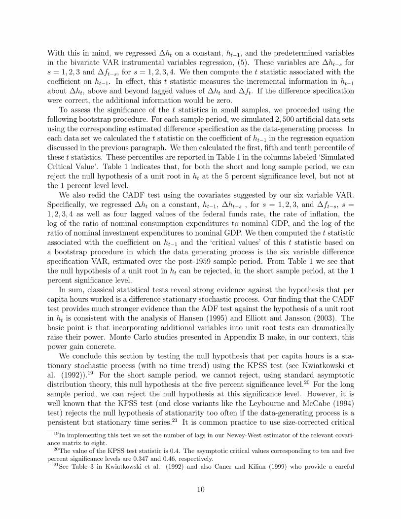
With this in mind, we regressed ∆ht on a constant, ht−1, and the predetermined variablesin the bivariate VAR instrumental variables regression, (5). These variables are ∆ht−s fors = 1, 2, 3 and ∆ft−s, for s = 1, 2, 3, 4. We then compute the t statistic associated with thecoefficient on ht−1. In effect, this t statistic measures the incremental information in ht−1about ∆ht, above and beyond lagged values of ∆ht and ∆ft. If the difference specificationwere correct, the additional information would be zero.To assess the significance of the t statistics in small samples, we proceeded using the

following bootstrap procedure. For each sample period, we simulated 2, 500 artificial data setsusing the corresponding estimated difference specification as the data-generating process. Ineach data set we calculated the t statistic on the coefficient of ht−1 in the regression equationdiscussed in the previous paragraph. We then calculated the first, fifth and tenth percentile ofthese t statistics. These percentiles are reported in Table 1 in the columns labeled ‘SimulatedCritical Value’. Table 1 indicates that, for both the short and long sample period, we canreject the null hypothesis of a unit root in ht at the 5 percent significance level, but not atthe 1 percent level level.We also redid the CADF test using the covariates suggested by our six variable VAR.

Specifically, we regressed ∆ht on a constant, ht−1, ∆ht−s , for s = 1, 2, 3, and ∆ft−s, s =1, 2, 3, 4 as well as four lagged values of the federal funds rate, the rate of inflation, thelog of the ratio of nominal consumption expenditures to nominal GDP, and the log of theratio of nominal investment expenditures to nominal GDP. We then computed the t statisticassociated with the coefficient on ht−1 and the ‘critical values’ of this t statistic based ona bootstrap procedure in which the data generating process is the six variable differencespecification VAR, estimated over the post-1959 sample period. From Table 1 we see thatthe null hypothesis of a unit root in ht can be rejected, in the short sample period, at the 1percent significance level.In sum, classical statistical tests reveal strong evidence against the hypothesis that per

capita hours worked is a difference stationary stochastic process. Our finding that the CADFtest provides much stronger evidence than the ADF test against the hypothesis of a unit rootin ht is consistent with the analysis of Hansen (1995) and Elliott and Jansson (2003). Thebasic point is that incorporating additional variables into unit root tests can dramaticallyraise their power. Monte Carlo studies presented in Appendix B make, in our context, thispower gain concrete.We conclude this section by testing the null hypothesis that per capita hours is a sta-

tionary stochastic process (with no time trend) using the KPSS test (see Kwiatkowski etal. (1992)).19 For the short sample period, we cannot reject, using standard asymptoticdistribution theory, this null hypothesis at the five percent significance level.20 For the longsample period, we can reject the null hypothesis at this significance level. However, it iswell known that the KPSS test (and close variants like the Leybourne and McCabe (1994)test) rejects the null hypothesis of stationarity too often if the data-generating process is apersistent but stationary time series.21 It is common practice to use size-corrected critical

19In implementing this test we set the number of lags in our Newey-West estimator of the relevant covari-ance matrix to eight.20The value of the KPSS test statistic is 0.4. The asymptotic critical values corresponding to ten and five

percent significance levels are 0.347 and 0.46, respectively.21See Table 3 in Kwiatkowski et al. (1992) and also Caner and Kilian (1999) who provide a careful

10

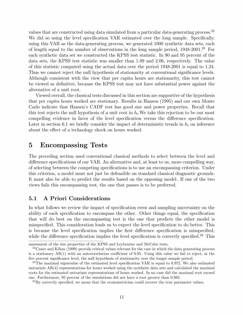
values that are constructed using data simulated from a particular data-generating process.22

We did so using the level specification VAR estimated over the long sample. Specifically,using this VAR as the data-generating process, we generated 1000 synthetic data sets, eachof length equal to the number of observations in the long sample period, 1948-2001.23 Foreach synthetic data set we constructed the KPSS test statistic. In 90 and 95 percent of thedata sets, the KPSS test statistic was smaller than 1.89 and 2.06, respectively. The valueof this statistic computed using the actual data over the period 1948-2001 is equal to 1.24.Thus we cannot reject the null hypothesis of stationarity at conventional significance levels.Although consistent with the view that per capita hours are stationarity, this test cannotbe viewed as definitive, because the KPSS test may not have substantial power against thealternative of a unit root.Viewed overall, the classical tests discussed in this section are supportive of the hypothesis

that per capita hours worked are stationary. Results in Hansen (1995) and our own MonteCarlo indicate that Hansen’s CADF test has good size and power properties. Recall thatthis test rejects the null hypothesis of a unit root in ht.We take this rejection to be our mostcompelling evidence in favor of the level specification versus the difference specification.Later in section 6.1 we briefly consider the impact of deterministic trends in ht on inferenceabout the effect of a technology shock on hours worked.

5 Encompassing Tests

The preceding section used conventional classical methods to select between the level anddifference specifications of our VAR. An alternative and, at least to us, more compelling way,of selecting between the competing specifications is to use an encompassing criterion. Underthis criterion, a model must not just be defensible on standard classical diagnostic grounds.It must also be able to predict the results based on the opposing model. If one of the twoviews fails this encompassing test, the one that passes is to be preferred.

5.1 A Priori Considerations

In what follows we review the impact of specification error and sampling uncertainty on theability of each specification to encompass the other. Other things equal, the specificationthat will do best on the encompassing test is the one that predicts the other model ismisspecified. This consideration leads us to expect the level specification to do better. Thisis because the level specification implies the first difference specification is misspecified,while the difference specification implies the level specification is correctly specified.24 This

assessment of the size properties of the KPSS and Leybourne and McCabe tests.22Caner and Kilian (1999) provide critical values relevant for the case in which the data generating process

is a stationary AR(1) with an autocorrelation coefficient of 0.95. Using this value we fail to reject, at thefive percent significance level, the null hypothesis of stationarity over the longer sample period.23The maximal eigenvalue of the estimated level specification VAR is equal to 0.972. We also estimated

univariate AR(4) representations for hours worked using the synthetic data sets and calculated the maximalroots for the estimated univariate representations of hours worked. In no case did the maximal root exceedone. Furthermore, 95 percent of the simulations did not have a root greater than 0.982.24By correctly specified, we mean that the econometrician could recover the true parameter values.

11

consideration is not definitive because sampling considerations also enter. For example, thedifference specification implies that the level specification suffers from a weak instrumentproblem. Weak instruments can lead to large sampling uncertainty as well as bias. Theseconsiderations may help the difference specification.

5.1.1 Level Specification

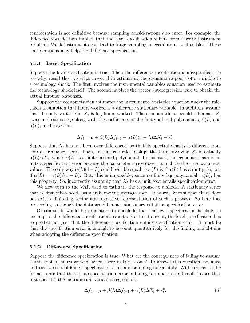
Suppose the level specification is true. Then the difference specification is misspecified. Tosee why, recall the two steps involved in estimating the dynamic response of a variable toa technology shock. The first involves the instrumental variables equation used to estimatethe technology shock itself. The second involves the vector autoregression used to obtain theactual impulse responses.Suppose the econometrician estimates the instrumental variables equation under the mis-

taken assumption that hours worked is a difference stationary variable. In addition, assumethat the only variable in Xt is log hours worked. The econometrician would difference Xttwice and estimate µ along with the coefficients in the finite-ordered polynomials, β(L) andα(L), in the system:

∆ft = µ+ β(L)∆ft−1 + α(L)(1− L)∆Xt + εzt .

Suppose that Xt has not been over differenced, so that its spectral density is different fromzero at frequency zero. Then, in the true relationship, the term involving Xt is actuallyα(L)∆Xt, where α(L) is a finite ordered polynomial. In this case, the econometrician com-mits a specification error because the parameter space does not include the true parametervalues. The only way α(L)(1−L) could ever be equal to α(L) is if α(L) has a unit pole, i.e.,if α(L) = α(L)/(1 − L). But, this is impossible, since no finite lag polynomial, α(L), hasthis property. So, incorrectly assuming that Xt has a unit root entails specification error.We now turn to the VAR used to estimate the response to a shock. A stationary series

that is first differenced has a unit moving average root. It is well known that there doesnot exist a finite-lag vector autoregressive representation of such a process. So here too,proceeding as though the data are difference stationary entails a specification error.Of course, it would be premature to conclude that the level specification is likely to

encompass the difference specification’s results. For this to occur, the level specification hasto predict not just that the difference specification entails specification error. It must bethat the specification error is enough to account quantitatively for the finding one obtainswhen adopting the difference specification.

5.1.2 Difference Specification

Suppose the difference specification is true. What are the consequences of failing to assumea unit root in hours worked, when there in fact is one? To answer this question, we mustaddress two sets of issues: specification error and sampling uncertainty. With respect to theformer, note that there is no specification error in failing to impose a unit root. To see this,first consider the instrumental variables regression:

∆ft = µ+ β(L)∆ft−1 + α(L)∆Xt + εzt . (5)

12

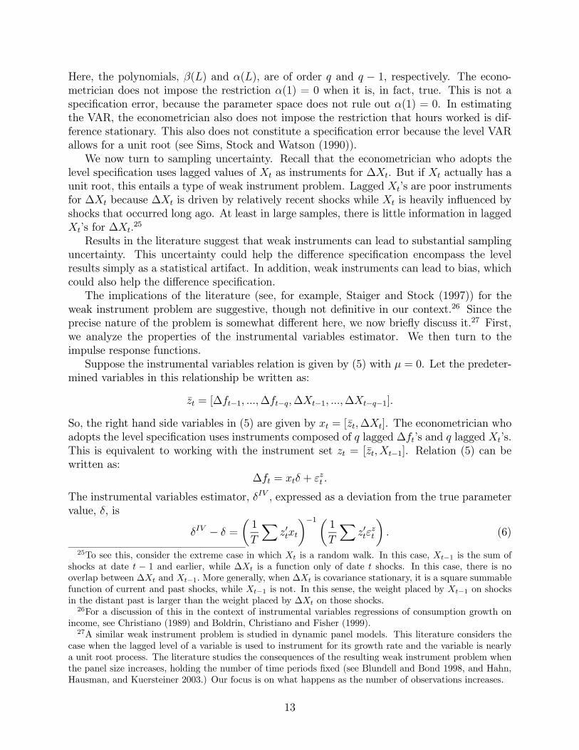
Here, the polynomials, β(L) and α(L), are of order q and q − 1, respectively. The econo-metrician does not impose the restriction α(1) = 0 when it is, in fact, true. This is not aspecification error, because the parameter space does not rule out α(1) = 0. In estimatingthe VAR, the econometrician also does not impose the restriction that hours worked is dif-ference stationary. This also does not constitute a specification error because the level VARallows for a unit root (see Sims, Stock and Watson (1990)).We now turn to sampling uncertainty. Recall that the econometrician who adopts the

level specification uses lagged values of Xt as instruments for ∆Xt. But if Xt actually has aunit root, this entails a type of weak instrument problem. Lagged Xt’s are poor instrumentsfor ∆Xt because ∆Xt is driven by relatively recent shocks while Xt is heavily influenced byshocks that occurred long ago. At least in large samples, there is little information in laggedXt’s for ∆Xt.

25

Results in the literature suggest that weak instruments can lead to substantial samplinguncertainty. This uncertainty could help the difference specification encompass the levelresults simply as a statistical artifact. In addition, weak instruments can lead to bias, whichcould also help the difference specification.The implications of the literature (see, for example, Staiger and Stock (1997)) for the

weak instrument problem are suggestive, though not definitive in our context.26 Since theprecise nature of the problem is somewhat different here, we now briefly discuss it.27 First,we analyze the properties of the instrumental variables estimator. We then turn to theimpulse response functions.Suppose the instrumental variables relation is given by (5) with µ = 0. Let the predeter-

mined variables in this relationship be written as:

zt = [∆ft−1, ...,∆ft−q,∆Xt−1, ...,∆Xt−q−1].

So, the right hand side variables in (5) are given by xt = [zt,∆Xt]. The econometrician whoadopts the level specification uses instruments composed of q lagged ∆ft’s and q lagged Xt’s.This is equivalent to working with the instrument set zt = [zt,Xt−1]. Relation (5) can bewritten as:

∆ft = xtδ + εzt .

The instrumental variables estimator, δIV , expressed as a deviation from the true parametervalue, δ, is

δIV − δ =

µ1

T

Xz0txt

¶−1µ1

T

Xz0tε

zt

¶. (6)

25To see this, consider the extreme case in which Xt is a random walk. In this case, Xt−1 is the sum ofshocks at date t − 1 and earlier, while ∆Xt is a function only of date t shocks. In this case, there is nooverlap between ∆Xt and Xt−1. More generally, when ∆Xt is covariance stationary, it is a square summablefunction of current and past shocks, while Xt−1 is not. In this sense, the weight placed by Xt−1 on shocksin the distant past is larger than the weight placed by ∆Xt on those shocks.26For a discussion of this in the context of instrumental variables regressions of consumption growth on

income, see Christiano (1989) and Boldrin, Christiano and Fisher (1999).27A similar weak instrument problem is studied in dynamic panel models. This literature considers the

case when the lagged level of a variable is used to instrument for its growth rate and the variable is nearlya unit root process. The literature studies the consequences of the resulting weak instrument problem whenthe panel size increases, holding the number of time periods fixed (see Blundell and Bond 1998, and Hahn,Hausman, and Kuersteiner 2003.) Our focus is on what happens as the number of observations increases.

13

HerePsignifies summation over t = 1, ..., T. To simplify notation, we also do not index the

estimator, δIV , by T . Relation (6) implies

δIV − δ =

·1T

Pz0tzt

1T

Pz0t∆Xt

1T

PXt−1zt 1

T

PXt−1∆Xt

¸−1 · 1T

Pz0tε

zt

1T

PXt−1εzt

¸L→·Qzz Qz∆Xϕ ζ

¸−1µ0%

¶,

where ‘L→’ signifies ‘converges in distribution’. Here, ϕ, ζ and % are well defined random

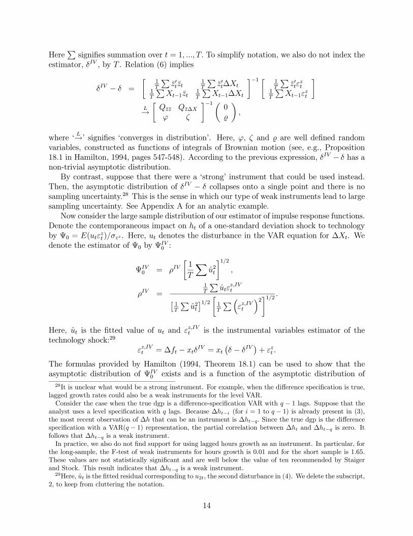
variables, constructed as functions of integrals of Brownian motion (see, e.g., Proposition18.1 in Hamilton, 1994, pages 547-548). According to the previous expression, δIV − δ has anon-trivial asymptotic distribution.By contrast, suppose that there were a ‘strong’ instrument that could be used instead.

Then, the asymptotic distribution of δIV − δ collapses onto a single point and there is nosampling uncertainty.28 This is the sense in which our type of weak instruments lead to largesampling uncertainty. See Appendix A for an analytic example.Now consider the large sample distribution of our estimator of impulse response functions.

Denote the contemporaneous impact on ht of a one-standard deviation shock to technologyby Ψ0 = E(utε

zt )/σεz . Here, ut denotes the disturbance in the VAR equation for ∆Xt. We

denote the estimator of Ψ0 by ΨIV0 :

ΨIV0 = ρIV

·1

T

Xu2t

¸1/2,

ρIV =1T

Putε

z,IVt£

1T

Pu2t¤1/2 · 1

T

P³εz,IVt

´2¸1/2 .Here, ut is the fitted value of ut and εz,IVt is the instrumental variables estimator of thetechnology shock:29

εz,IVt = ∆ft − xtδIV = xt¡δ − δIV

¢+ εzt .

The formulas provided by Hamilton (1994, Theorem 18.1) can be used to show that theasymptotic distribution of ΨIV

0 exists and is a function of the asymptotic distribution of

28It is unclear what would be a strong instrument. For example, when the difference specification is true,lagged growth rates could also be a weak instruments for the level VAR.Consider the case when the true dgp is a difference-specification VAR with q − 1 lags. Suppose that the

analyst uses a level specification with q lags. Because ∆ht−i (for i = 1 to q − 1) is already present in (3),the most recent observation of ∆h that can be an instrument is ∆ht−q. Since the true dgp is the differencespecification with a VAR(q − 1) representation, the partial correlation between ∆ht and ∆ht−q is zero. Itfollows that ∆ht−q is a weak instrument.In practice, we also do not find support for using lagged hours growth as an instrument. In particular, for

the long-sample, the F-test of weak instruments for hours growth is 0.01 and for the short sample is 1.65.These values are not statistically significant and are well below the value of ten recommended by Staigerand Stock. This result indicates that ∆ht−q is a weak instrument.29Here, ut is the fitted residual corresponding to u2t, the second disturbance in (4). We delete the subscript,

2, to keep from cluttering the notation.

14

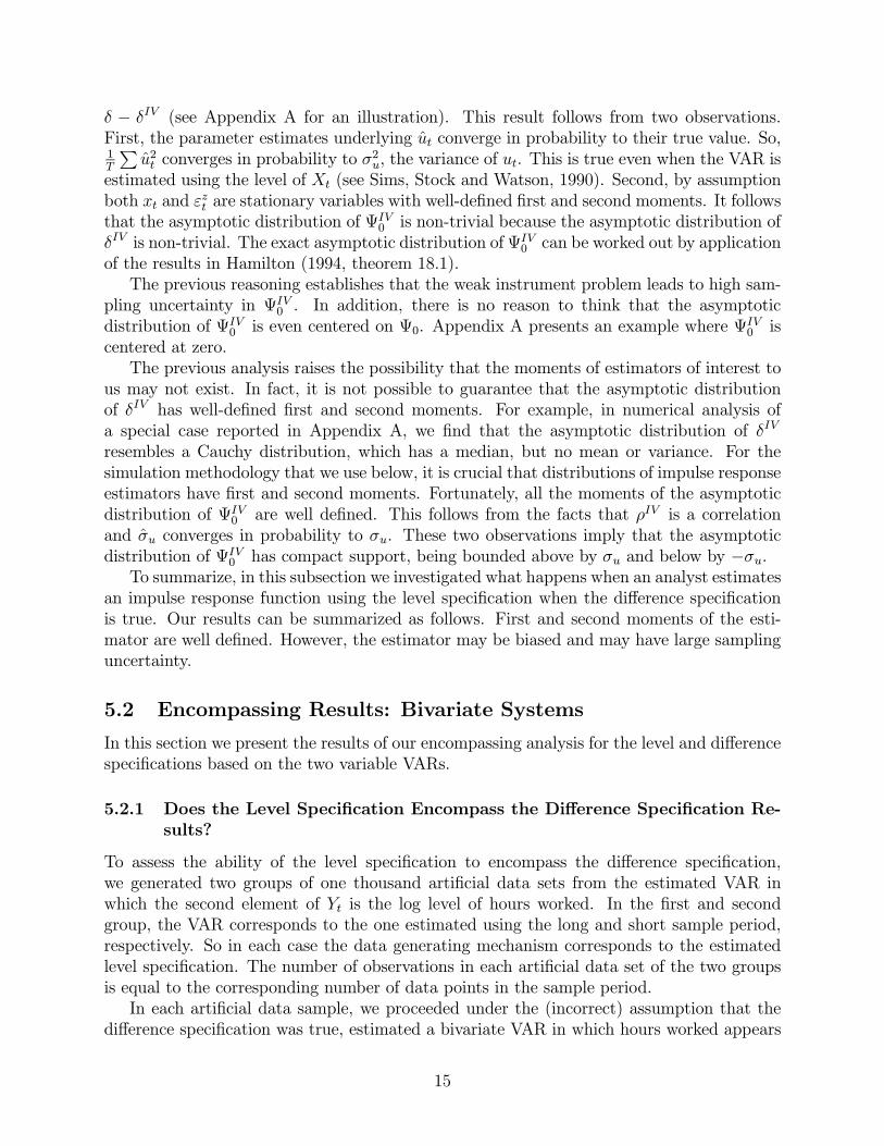
δ − δIV (see Appendix A for an illustration). This result follows from two observations.First, the parameter estimates underlying ut converge in probability to their true value. So,1T

Pu2t converges in probability to σ

2u, the variance of ut. This is true even when the VAR is

estimated using the level of Xt (see Sims, Stock and Watson, 1990). Second, by assumptionboth xt and ε

zt are stationary variables with well-defined first and second moments. It follows

that the asymptotic distribution of ΨIV0 is non-trivial because the asymptotic distribution of

δIV is non-trivial. The exact asymptotic distribution ofΨIV0 can be worked out by application

of the results in Hamilton (1994, theorem 18.1).The previous reasoning establishes that the weak instrument problem leads to high sam-

pling uncertainty in ΨIV0 . In addition, there is no reason to think that the asymptoticdistribution of ΨIV

0 is even centered on Ψ0. Appendix A presents an example where ΨIV0 is

centered at zero.The previous analysis raises the possibility that the moments of estimators of interest to

us may not exist. In fact, it is not possible to guarantee that the asymptotic distributionof δIV has well-defined first and second moments. For example, in numerical analysis ofa special case reported in Appendix A, we find that the asymptotic distribution of δIV

resembles a Cauchy distribution, which has a median, but no mean or variance. For thesimulation methodology that we use below, it is crucial that distributions of impulse responseestimators have first and second moments. Fortunately, all the moments of the asymptoticdistribution of ΨIV0 are well defined. This follows from the facts that ρIV is a correlationand σu converges in probability to σu. These two observations imply that the asymptoticdistribution of ΨIV

0 has compact support, being bounded above by σu and below by −σu.To summarize, in this subsection we investigated what happens when an analyst estimates

an impulse response function using the level specification when the difference specificationis true. Our results can be summarized as follows. First and second moments of the esti-mator are well defined. However, the estimator may be biased and may have large samplinguncertainty.

5.2 Encompassing Results: Bivariate Systems

In this section we present the results of our encompassing analysis for the level and differencespecifications based on the two variable VARs.

5.2.1 Does the Level Specification Encompass the Difference Specification Re-sults?

To assess the ability of the level specification to encompass the difference specification,we generated two groups of one thousand artificial data sets from the estimated VAR inwhich the second element of Yt is the log level of hours worked. In the first and secondgroup, the VAR corresponds to the one estimated using the long and short sample period,respectively. So in each case the data generating mechanism corresponds to the estimatedlevel specification. The number of observations in each artificial data set of the two groupsis equal to the corresponding number of data points in the sample period.In each artificial data sample, we proceeded under the (incorrect) assumption that the

difference specification was true, estimated a bivariate VAR in which hours worked appears

15

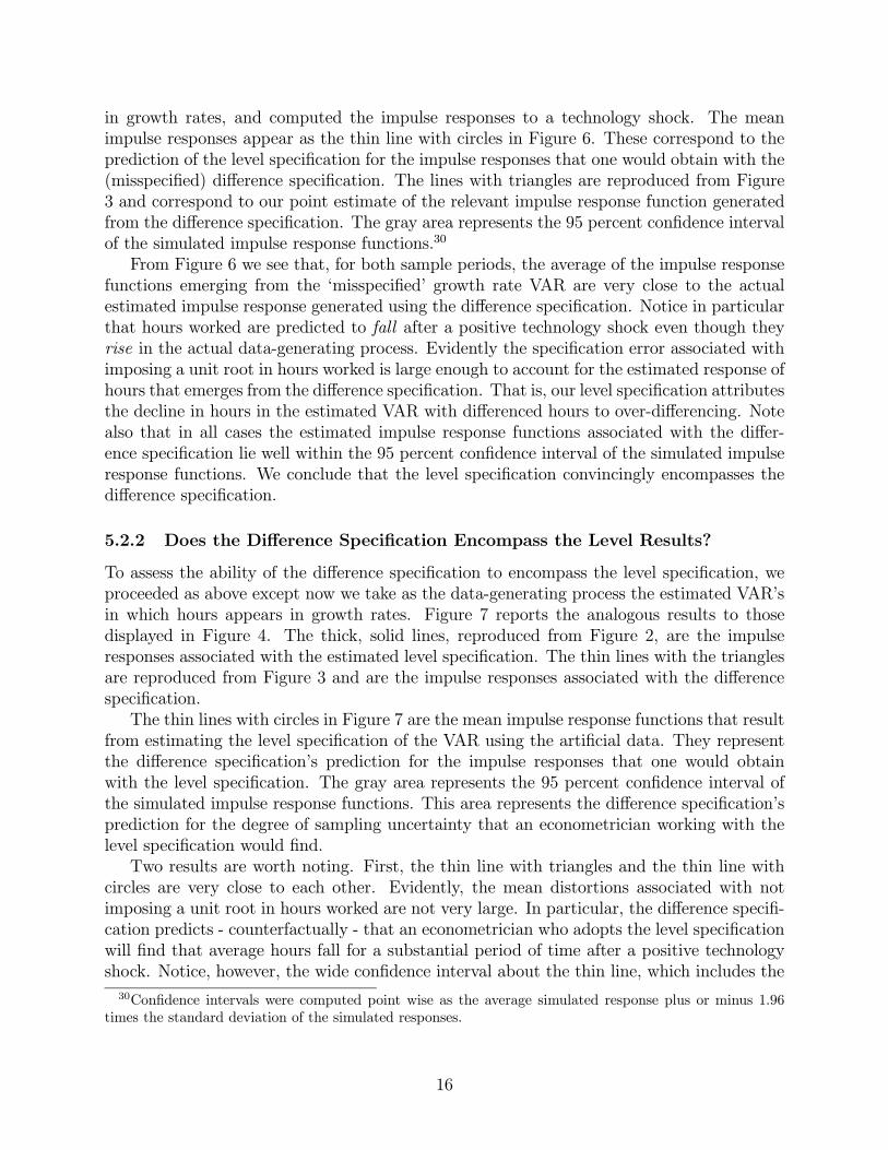
in growth rates, and computed the impulse responses to a technology shock. The meanimpulse responses appear as the thin line with circles in Figure 6. These correspond to theprediction of the level specification for the impulse responses that one would obtain with the(misspecified) difference specification. The lines with triangles are reproduced from Figure3 and correspond to our point estimate of the relevant impulse response function generatedfrom the difference specification. The gray area represents the 95 percent confidence intervalof the simulated impulse response functions.30

From Figure 6 we see that, for both sample periods, the average of the impulse responsefunctions emerging from the ‘misspecified’ growth rate VAR are very close to the actualestimated impulse response generated using the difference specification. Notice in particularthat hours worked are predicted to fall after a positive technology shock even though theyrise in the actual data-generating process. Evidently the specification error associated withimposing a unit root in hours worked is large enough to account for the estimated response ofhours that emerges from the difference specification. That is, our level specification attributesthe decline in hours in the estimated VAR with differenced hours to over-differencing. Notealso that in all cases the estimated impulse response functions associated with the differ-ence specification lie well within the 95 percent confidence interval of the simulated impulseresponse functions. We conclude that the level specification convincingly encompasses thedifference specification.

5.2.2 Does the Difference Specification Encompass the Level Results?

To assess the ability of the difference specification to encompass the level specification, weproceeded as above except now we take as the data-generating process the estimated VAR’sin which hours appears in growth rates. Figure 7 reports the analogous results to thosedisplayed in Figure 4. The thick, solid lines, reproduced from Figure 2, are the impulseresponses associated with the estimated level specification. The thin lines with the trianglesare reproduced from Figure 3 and are the impulse responses associated with the differencespecification.The thin lines with circles in Figure 7 are the mean impulse response functions that result

from estimating the level specification of the VAR using the artificial data. They representthe difference specification’s prediction for the impulse responses that one would obtainwith the level specification. The gray area represents the 95 percent confidence interval ofthe simulated impulse response functions. This area represents the difference specification’sprediction for the degree of sampling uncertainty that an econometrician working with thelevel specification would find.Two results are worth noting. First, the thin line with triangles and the thin line with

circles are very close to each other. Evidently, the mean distortions associated with notimposing a unit root in hours worked are not very large. In particular, the difference specifi-cation predicts - counterfactually - that an econometrician who adopts the level specificationwill find that average hours fall for a substantial period of time after a positive technologyshock. Notice, however, the wide confidence interval about the thin line, which includes the

30Confidence intervals were computed point wise as the average simulated response plus or minus 1.96times the standard deviation of the simulated responses.

16

thick, solid line. So, the difference specification can account for the point estimates basedon the level specification, but only as an accident of sampling uncertainty.At the same time, the prediction of large sampling uncertainty poses important challenges

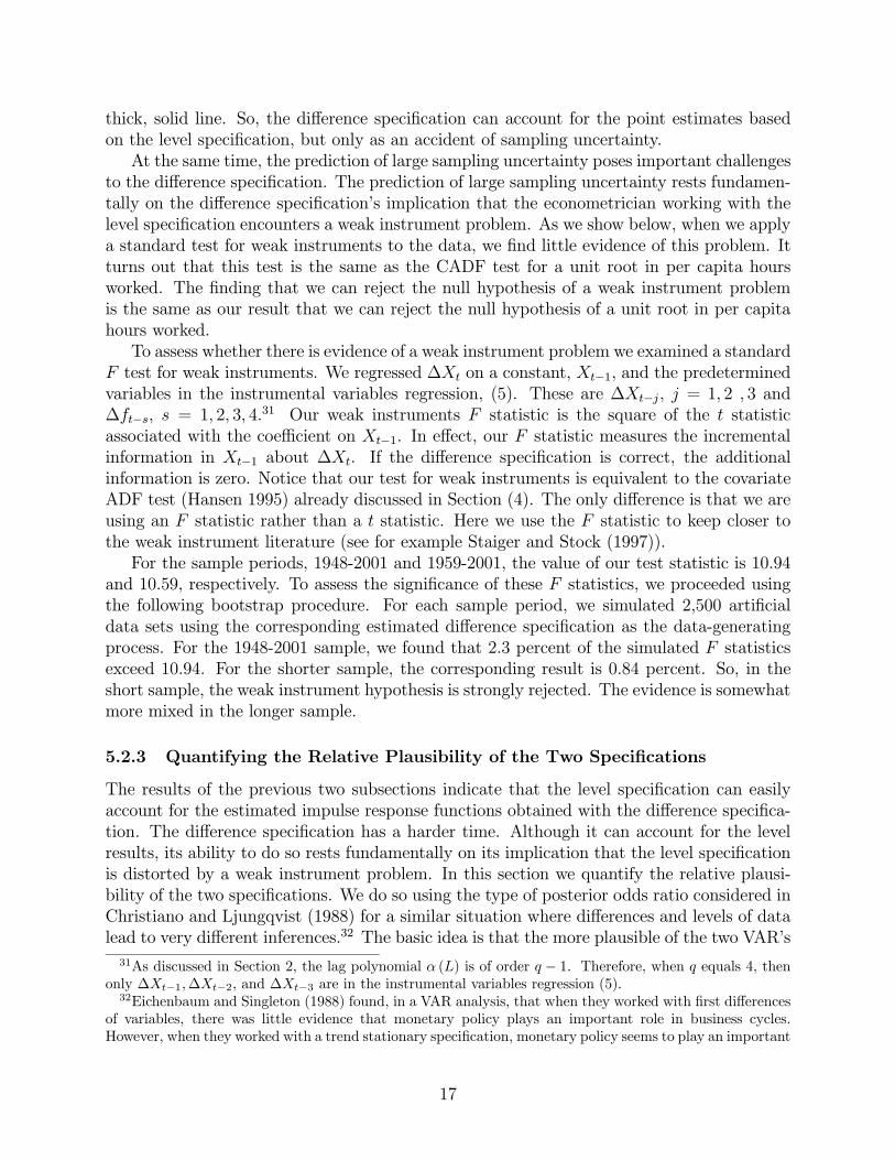
to the difference specification. The prediction of large sampling uncertainty rests fundamen-tally on the difference specification’s implication that the econometrician working with thelevel specification encounters a weak instrument problem. As we show below, when we applya standard test for weak instruments to the data, we find little evidence of this problem. Itturns out that this test is the same as the CADF test for a unit root in per capita hoursworked. The finding that we can reject the null hypothesis of a weak instrument problemis the same as our result that we can reject the null hypothesis of a unit root in per capitahours worked.To assess whether there is evidence of a weak instrument problem we examined a standard

F test for weak instruments. We regressed ∆Xt on a constant, Xt−1, and the predeterminedvariables in the instrumental variables regression, (5). These are ∆Xt−j, j = 1, 2 , 3 and∆ft−s, s = 1, 2, 3, 4.31 Our weak instruments F statistic is the square of the t statisticassociated with the coefficient on Xt−1. In effect, our F statistic measures the incrementalinformation in Xt−1 about ∆Xt. If the difference specification is correct, the additionalinformation is zero. Notice that our test for weak instruments is equivalent to the covariateADF test (Hansen 1995) already discussed in Section (4). The only difference is that we areusing an F statistic rather than a t statistic. Here we use the F statistic to keep closer tothe weak instrument literature (see for example Staiger and Stock (1997)).For the sample periods, 1948-2001 and 1959-2001, the value of our test statistic is 10.94

and 10.59, respectively. To assess the significance of these F statistics, we proceeded usingthe following bootstrap procedure. For each sample period, we simulated 2,500 artificialdata sets using the corresponding estimated difference specification as the data-generatingprocess. For the 1948-2001 sample, we found that 2.3 percent of the simulated F statisticsexceed 10.94. For the shorter sample, the corresponding result is 0.84 percent. So, in theshort sample, the weak instrument hypothesis is strongly rejected. The evidence is somewhatmore mixed in the longer sample.

5.2.3 Quantifying the Relative Plausibility of the Two Specifications

The results of the previous two subsections indicate that the level specification can easilyaccount for the estimated impulse response functions obtained with the difference specifica-tion. The difference specification has a harder time. Although it can account for the levelresults, its ability to do so rests fundamentally on its implication that the level specificationis distorted by a weak instrument problem. In this section we quantify the relative plausi-bility of the two specifications. We do so using the type of posterior odds ratio considered inChristiano and Ljungqvist (1988) for a similar situation where differences and levels of datalead to very different inferences.32 The basic idea is that the more plausible of the two VAR’s

31As discussed in Section 2, the lag polynomial α (L) is of order q − 1. Therefore, when q equals 4, thenonly ∆Xt−1,∆Xt−2, and ∆Xt−3 are in the instrumental variables regression (5).32Eichenbaum and Singleton (1988) found, in a VAR analysis, that when they worked with first differences

of variables, there was little evidence that monetary policy plays an important role in business cycles.However, when they worked with a trend stationary specification, monetary policy seems to play an important

17

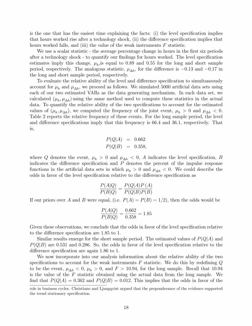
is the one that has the easiest time explaining the facts: (i) the level specification impliesthat hours worked rise after a technology shock, (ii) the difference specification implies thathours worked falls, and (iii) the value of the weak instruments F statistic.We use a scalar statistic - the average percentage change in hours in the first six periods

after a technology shock - to quantify our findings for hours worked. The level specificationestimates imply this change, µh,is equal to 0.89 and 0.55 for the long and short sampleperiod, respectively. The analogous statistic, µ∆h, for the difference is −0.13 and −0.17 inthe long and short sample period, respectively.To evaluate the relative ability of the level and difference specification to simultaneously

account for µh and µ∆h, we proceed as follows. We simulated 5000 artificial data sets usingeach of our two estimated VARs as the data generating mechanism. In each data set, wecalculated (µh, µ∆h) using the same method used to compute these statistics in the actualdata. To quantify the relative ability of the two specifications to account for the estimatedvalues of (µh, µ∆h), we computed the frequency of the joint event, µh > 0 and µ∆h < 0.Table 2 reports the relative frequency of these events. For the long sample period, the leveland difference specifications imply that this frequency is 66.4 and 36.1, respectively. Thatis,

P (Q|A) = 0.662

P (Q|B) = 0.358,

where Q denotes the event, µh > 0 and µ∆h < 0, A indicates the level specification, Bindicates the difference specification and P denotes the percent of the impulse responsefunctions in the artificial data sets in which µh > 0 and µ∆h < 0. We could describe theodds in favor of the level specification relative to the difference specification as

P (A|Q)P (B|Q) =

P (Q|A)P (A)P (Q|B)P (B)

If our priors over A and B were equal, (i.e. P (A) = P (B) = 1/2), then the odds would be

P (A|Q)P (B|Q) =

0.662

0.358= 1.85

Given these observations, we conclude that the odds in favor of the level specification relativeto the difference specification are 1.85 to 1.Similar results emerge for the short sample period. The estimated values of P (Q|A) and

P (Q|B) are 0.531 and 0.286. So, the odds in favor of the level specification relative to thedifference specification are again 1.86 to 1.We now incorporate into our analysis information about the relative ability of the two

specifications to account for the weak instruments F statistic. We do this by redefining Qto be the event, µ∆h < 0, µh > 0, and F > 10.94, for the long sample. Recall that 10.94is the value of the F statistic obtained using the actual data from the long sample. Wefind that P (Q|A) = 0.362 and P (Q|B) = 0.012. This implies that the odds in favor of therole in business cycles. Christiano and Ljungqvist argued that the preponderance of the evidence supportedthe trend stationary specification.

18

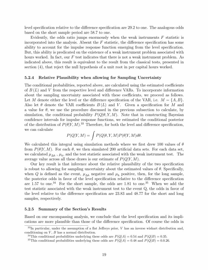
level specification relative to the difference specification are 29.2 to one. The analogous oddsbased on the short sample period are 58.7 to one.Evidently, the odds ratio jumps enormously when the weak instruments F statistic is

incorporated into the analysis. Absent the F statistic, the difference specification has someability to account for the impulse response function emerging from the level specification.But, this ability is predicated on the existence of a weak instrument problem associated withhours worked. In fact, our F test indicates that there is not a weak instrument problem. Asindicated above, this result is equivalent to the result from the classical tests, presented insection (4), that reject the null hypothesis of a unit root in per capital hours worked.

5.2.4 Relative Plausibility when allowing for Sampling Uncertainty

The conditional probabilities, reported above, are calculated using the estimated coefficientsof B (L) and V from the respective level and difference VARs. To incorporate informationabout the sampling uncertainty associated with these coefficients, we proceed as follows.Let M denote either the level or the difference specification of the VAR, i.e. M = {A,B}.Also let θ denote the VAR coefficients B (L) and V . Given a specification for M anda value for θ, we use the procedure discussed in the previous subsection to calculate, bysimulation, the conditional probability P (Q|θ, Y,M). Note that in constructing Bayesianconfidence intervals for impulse response functions, we estimated the conditional posteriorof the distribution of P (θ|Y,M).33 Therefore, for both the level and difference specification,we can calculate

P (Q|Y,M) =ZP (Q|θ, Y,M)P (θ|Y,M)dθ.

We calculated this integral using simulation methods where we first drew 100 values of θfrom P (θ|Y,M). For each θ, we then simulated 200 artificial data sets. For each data set,we calculated µ∆h , µh, and the test statistic associated with the weak instrument test. Theaverage value across all these draws is our estimate of P (Q|Y,M).Our key result is that inference about the relative plausibility of the two specification

is robust to allowing for sampling uncertainty about the estimated values of θ. Specifically,when Q is defined as the event, µ∆h negative and µh positive, then, for the long sample,the posterior odds in favor of the level specification relative to the difference specificationare 1.57 to one.34 For the short sample, the odds are 1.81 to one.35 When we add thetest statistic associated with the weak instrument test to the event Q, the odds in favor ofthe level relative to the difference specification are 23.83 and 48.77 for the short and longsamples, respectively.

5.2.5 Summary of the Section’s Results

Based on our encompassing analysis, we conclude that the level specification and its impli-cations are more plausible than those of the difference specification. Of course the odds in

33In particular, under the assumption of a flat Jeffreys prior, V has an inverse wishart distribution and,conditioning on V , B has a normal distribution.34This conditional probabilities underlying these odds are P (Q|A) = 0.54 and P (Q|B) = 0.35.35This conditional probabilities underlying these odds are P (Q|A) = 0.48 and P (Q|B) = 0.0.26.

19

favor of the level specification would be even higher if we assigned more prior weight to thelevel specification. For reasons discussed in the introduction this seems quite natural to us.Our own prior is that the difference specification simply cannot be true because per capitahours worked are bounded.

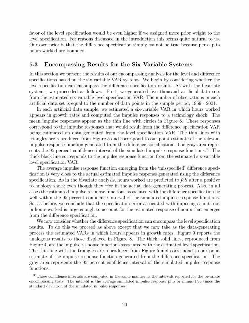
5.3 Encompassing Results for the Six Variable Systems

In this section we present the results of our encompassing analysis for the level and differencespecifications based on the six variable VAR systems. We begin by considering whether thelevel specification can encompass the difference specification results. As with the bivariatesystems, we proceeded as follows. First, we generated five thousand artificial data setsfrom the estimated six-variable level specification VAR. The number of observations in eachartificial data set is equal to the number of data points in the sample period, 1959 - 2001.In each artificial data sample, we estimated a six-variable VAR in which hours worked

appears in growth rates and computed the impulse responses to a technology shock. Themean impulse responses appear as the thin line with circles in Figure 8. These responsescorrespond to the impulse responses that would result from the difference specification VARbeing estimated on data generated from the level specification VAR. The thin lines withtriangles are reproduced from Figure 5 and correspond to our point estimate of the relevantimpulse response function generated from the difference specification. The gray area repre-sents the 95 percent confidence interval of the simulated impulse response functions.36 Thethick black line corresponds to the impulse response function from the estimated six-variablelevel specification VAR.The average impulse response function emerging from the ‘misspecified’ difference speci-

fication is very close to the actual estimated impulse response generated using the differencespecification. As in the bivariate analysis, hours worked are predicted to fall after a positivetechnology shock even though they rise in the actual data-generating process. Also, in allcases the estimated impulse response functions associated with the difference specification liewell within the 95 percent confidence interval of the simulated impulse response functions.So, as before, we conclude that the specification error associated with imposing a unit rootin hours worked is large enough to account for the estimated response of hours that emergesfrom the difference specification.We now consider whether the difference specification can encompass the level specification

results. To do this we proceed as above except that we now take as the data-generatingprocess the estimated VARs in which hours appears in growth rates. Figure 9 reports theanalogous results to those displayed in Figure 8. The thick, solid lines, reproduced fromFigure 4, are the impulse response functions associated with the estimated level specification.The thin line with the triangles are reproduced from Figure 5 and correspond to our pointestimate of the impulse response function generated from the difference specification. Thegray area represents the 95 percent confidence interval of the simulated impulse responsefunctions.

36These confidence intervals are computed in the same manner as the intervals reported for the bivariateencompassing tests. The interval is the average simulated impulse response plus or minus 1.96 times thestandard deviation of the simulated impulse responses.

20

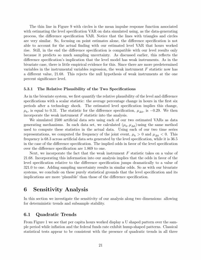
The thin line in Figure 9 with circles is the mean impulse response function associatedwith estimating the level specification VAR on data simulated using, as the data-generatingprocess, the difference specification VAR. Notice that the lines with triangles and circlesare very similar. So, focusing on point estimates alone, the difference specification is notable to account for the actual finding with our estimated level VAR that hours workedrise. Still, in the end the difference specification is compatible with our level results onlybecause it predicts so much sampling uncertainty. As discussed earlier, this reflects thedifference specification’s implication that the level model has weak instruments. As in thebivariate case, there is little empirical evidence for this. Since there are more predeterminedvariables in the instrumental variables regression, the weak instrument F statistic now hasa different value, 21.68. This rejects the null hypothesis of weak instruments at the onepercent significance level.

5.3.1 The Relative Plausibility of the Two Specifications

As in the bivariate system, we first quantify the relative plausibility of the level and differencespecifications with a scalar statistic: the average percentage change in hours in the first sixperiods after a technology shock. The estimated level specification implies this change,µh, is equal to 0.31. The statistic for the difference specification, µ∆h, is −0.29. We thenincorporate the weak instrument F statistic into the analysis.We simulated 2500 artificial data sets using each of our two estimated VARs as data

generating mechanisms. In each data set, we calculated (µh, µ∆h) using the same methodused to compute these statistics in the actual data. Using each of our two time seriesrepresentations, we computed the frequency of the joint event, µh > 0 and µ∆h < 0. Thisfrequency is 68.3 across artificial data sets generated by the level specification, while it is 36.5in the case of the difference specification. The implied odds in favor of the level specificationover the difference specification are 1.869 to one.Next, we incorporate the fact that the weak instrument F statistic takes on a value of

21.68. Incorporating this information into our analysis implies that the odds in favor of thelevel specification relative to the difference specification jumps dramatically to a value of321.0 to one. Adding sampling uncertainty results in similar odds. So as with our bivariatesystems, we conclude on these purely statistical grounds that the level specification and itsimplications are more ‘plausible’ than those of the difference specification.

6 Sensitivity Analysis

In this section we investigate the sensitivity of our analysis along two dimensions: allowingfor deterministic trends and subsample stability.

6.1 Quadratic Trends

From Figure 1 we see that per capita hours worked display a U shaped pattern over the sam-ple period while inflation and the federal funds rate exhibit hump-shaped patterns. Classicalstatistical tests appear to be consistent with the presence of quadratic trends in all three

21

variables. Specifically, we regressed the log of per capita hours worked, inflation and thefederal funds rate on a constant, time and time-squared using data over the sample period1959q1-2001q4. We then computed the t statistics for the time-squared terms allowing forserial correlation in the error term of the regressions using the standard Newey-West pro-cedure.37 The resulting t statistics are equal to 8.12, −4.62 and −4.23 for per capita hoursworked, inflation and the federal funds rate, respectively. Using standard asymptotic distri-bution theory, we can reject, at even the one percent significance level, the null hypothesisthat these quadratic time trend coefficients are equal to zero. So, on this basis, we wouldreject our level specification. But, it is well-known that the asymptotic distribution theoryfor this kind of t statistic is a poor approximation to the actual distribution in small samples.The approximation is particularly poor when the error terms exhibit high degrees of serialcorrelation, which is exactly the current situation according to our level model38

To address this concern, we adopt the following procedure. We simulate 2, 500 synthetictime series on all the variables in the VAR using our estimated level model. The disturbancesused in these simulations were randomly drawn from the fitted residuals of our estimatedlevel model. The length of each synthetic time series is equal to the length of our sampleperiod. We found that for the quadratic trend terms (i) 12.2 percent of the t statisticsassociated with per capita hours worked exceeded 8.12, (ii) 26.6 percent of the t statisticsassociated with inflation were smaller than −4.62, and (iii) 29.8 percent of the t statisticsassociated with the federal funds rate were smaller than −4.23. So, from the perspective ofthe level model, the estimated t statistics are not particularly unusual. So once we correct forthe small sample distribution of the t statistics, we fail to reject the null hypothesis that thecoefficients on the time-squared terms in per capita hours worked, inflation and the federalfunds equal zero.Of course, with these critical values, these tests may suffer from poor power. So it is

interesting to see how inference is affected by removing quadratic trends in the variablesfrom our VAR.39 To this end, we redid our analysis of the six-variable system with threetypes of quadratic trends. In case (i) we remove quadratic trends from all variables beforeestimating the VAR. In case (ii) we remove quadratic trends from per capita hours worked,inflation and the federal funds rate before estimating the VAR. Finally, in case (iii) we removea quadratic trend from only per capita hours worked before estimating the VAR. In all cases,variables not detrended enter into the VAR exactly as in the level specification.Figure 10 reports our results. The dark, thick lines correspond to the impulse response

functions implied by the six-variable level specification. The lines indicated with dots, starsand x’s correspond to the impulse response functions generated from the estimated versions ofcase (i), (ii) and (iii). The grey area is the 95 percent confidence interval associated with case(iii) where only hours have been detrended. We report only this confidence interval, ratherthan all three, to give a sense of sampling uncertainty while keeping the figure relativelysimple.Two things are worth noting. First, suppose we detrend all of the variables in the VAR

37We allow for serial correlation of order 12 in the Newey-West procedure.38The two largest eigenvalues of the determinant of [I −B(L)] in (4) are 0.9903 and 0.9126.39We redid our VAR analysis allowing for a linear trend in all equations of the six variable VAR. The re-

sulting impulse response functions are very similar to those associated with the six variable level specificationVAR.

22

(case i), or we detrend just per capita hours worked, inflation and the federal funds rate (caseii). Then after a small initial fall, hours worked rise in response to a positive technologyshock. In this sense, inference in the level specification is robust to allowing for quadratictrends. Second, if we allow for a quadratic trend only in per capita hours worked (case iii),then hours worked fall in a persistent way after a positive shock to technology. The problemwith this case is that it treats hours worked differently from the other variables in terms ofallowing for a quadratic trend. We see no rationale for this asymmetry. Consequently, weattach little importance to this last result.We conclude that inference regarding the effect of a technology shock on hours worked

is robust to allowing for quadratic trends in all the variables entering the analysis (casei) or just the subset of variables where a quadratic trend appears to be significant on thebasis of standard classical tests (case ii). To overturn the key result emerging from thelevel specification, it is necessary to treat hours worked asymmetrically from variables likeinflation and the federal funds rate that, over our sample, also exhibit quadratic-trend likebehavior.

6.1.1 Assessing the Relative Plausibility of the Different Models

We now briefly discuss the relative plausibility of the different models considered in theprevious subsection. Recall that when we only detrend hours worked (case (iii)), inferenceis different than when we work with the level specification. Since this is the only case inwhich inference is sensitive, we are particularly interest in the relative plausibility of case(iii). We proceed using a posterior odds ratio like the one in section 5.2.3. We focus on themodels’ ability to account for (a) the t statistics associated with standard classical tests forquadratic trends in per capita hours worked, inflation and the federal funds rate, and (b) thesign of the response of per capita hours worked to a technology shock in the different cases.Let µ1, µ2, µ3 and µ4 denote the average percentage change in per capita hours in the first

six periods after a technology shock in case (i), case (ii), case (iii) and the level specification(case iv), respectively The values of µ1, µ 2, µ3 and µ4 are equal to 0.15, 0.15, −0.12 and 0.31,respectively. Since µ1 and µ2 are the same, we do not include µ1 separately in calculating theposterior odds for the different cases. To calculating these odds we simulated 2500 artificialdata sets using each of our the four estimated VARs as data generating mechanisms. Ineach artificial data set, we calculated (µ2, µ3, µ4) using the same method used to computethese statistics in the actual data. For each data generating mechanism, we computed thefrequency of the joint event (µ2, µ4 > 0, µ3 < 0). The resulting frequencies are equal to 94,72 , 48 and 86 percent, for cases (i) - (iv), respectively. Using equally weighted priors overthe different cases, we then computed the posterior odds of case (i), (ii) and (iv) relative tocase (iii). The resulting odds are 1.97, 1.50 and 1.81 to one. So in every case - includingthe level specification (case iv) - the preponderance of the data favors the alternative to thespecification where we only detrend per capita hours worked (case (iv)).The weight of the evidence against case (iii) becomes overwhelming once we incorporate

the t statistics associated with the test of the quadratic trend terms in per capita hours,inflation and the federal funds rate into our analysis. We denote these t statistics by tD1 , t

D2

and tD3 , respectively. Recall these are equal to 8.12, −4.62 and −4.23, respectively.Using the simulated data from the four VAR’s, we computed t statistics for the quadratic

23

trend terms on per capita hours (tS1 ), inflation (tS2 ) and the federal funds rate (t

S3 ). Then

using the simulated data from our four estimated VAR’s, we computed the frequency of thejoint event, (µ2, µ4 > 0, µ3 < 0, tSi > tDi , i = 1, 2, 3) for each case. These frequencies areequal to 19, 8, 1 and 9 percent for cases (i) - (iv), respectively. Using equally weighted priorsover the different cases, we then computed the posterior odds of case (i), (ii) and (iv) relativeto case (iii). The resulting odds are 20.13, 7.92 and 3.79 to one. So in all cases - includingthe level specification (case iv)- the odds are very much against the specification in whichwe detrend only per capita hours worked (case (iii).To summarize, in all cases but one inference about the response of per capita hours

worked to a technology shock is robust to allowing for quadratic trends. The exception isthe case where we detrend only per capita hours worked. But the weight of the data stronglysupport the alternatives to that specification.

6.2 Subsample Stability

In this subsection we briefly discuss subsample stability, focusing on the six-variable levelspecification. Authors such as Gali, Lopez-Salido, and Valles (2002), among others, haveargued that monetary policy may have changed after 1979, and that this resulted in astructural change in VAR’s. Throughout our analysis, we have assumed implicitly thatthere has been no structural change. This section assesses the robustness of our conclusionsto the possibility of subsample instability.Figure 12 display the estimated impulse responses of the variables in our system to a

technology shock, for the pre-1979Q4 and post-1979Q3 sample periods. In addition, the fullsample impulse response and confidence intervals are reproduced from Figure 6.The key results are as follows. First, according to the point estimates, in the early

period hours worked fall for roughly three quarters before rising sharply in a hump-shapedpattern. In the late period, the estimated response of hours worked is similar to the estimatesbased on the full sample period. Second, the point estimates for each sample period lie wellwithin the 95 percent confidence intervals. This is consistent with the responses in thesubperiods being the same as they are for the full sample. The evidence is also consistentwith there being no break in the response of consumption and output. Third, there is someevidence of instability in the response of the interest rate and investment, in the early period.In particular, the decline in investment and in the interest rate are sufficiently large thatportions of their impulse response functions lie outside their respective confidence intervals.Likewise, in the late period, inflation falls much less than in the full sample. These initialdeclines are sufficiently large that if one applies a conventional F test for the null hypothesisof no sample break in the VAR, the hypothesis is rejected at the one percent significancelevel. This rejection notwithstanding, the key result from our perspective is that inferenceabout the response of hours worked to a technology shock is not affected by subsamplestability issues.

24

7 How Important Are Permanent Technology Shocks

for Aggregate Fluctuations?

In Section 4 and Section 5 we argued that the weight of the evidence favors the level specifi-cation relative to the difference specification. Here, we use the level specification to assess therole of technology shocks in aggregate fluctuations. We conclude that (i) technology shocksare not particularly important at business cycle frequencies but they do play an importantrole at relatively low frequencies of the data, and (ii) inference based on bivariate systemsgreatly overstates the cyclical importance of technology shocks.

7.1 Bivariate System Results

We begin by discussing the role of technology shocks in the variability of output and hoursworked based on our level specification bivariate VAR. Table 3 reports the percentage offorecast error variance due to technology shocks, at horizons of 1, 4, 8, 12, 20 and 50 quarters.By construction, permanent technology shocks account for all of the forecast error varianceof output at the infinite horizon. Notice that technology shocks account for an importantfraction of the variance of output at all reported horizons. For example, they account forroughly 80 percent of the one step ahead forecast error variance in output. In contrast, theyaccount for only a small percentage of the one step forecast error variance in hours worked(4.5 percent). But they account for a larger percentage of the forecast error variance in hoursworked at longer horizons, exceeding forty percent at horizons greater than two years.The first row of Table 5 reports the percentage of the variance in output and hours

worked at business cycle frequencies due to technology shocks. This statistic was computedas follows. First we simulated the estimated level specification bivariate VAR driven onlyby the estimated technology shocks. Next we computed the variance of the simulated dataafter applying the Hodrick-Prescott (HP) filter. Finally we computed the variance of theactual HP filtered output and hours worked. For any given variable, the ratio of the twovariances is our estimate of the fraction of business cycle variation in that variable due totechnology shocks. The results in Table 4 indicate that technology shocks appear to play asignificant role for both output and hours worked, accounting for roughly 64 and 33 percentof the cyclical variance in these two variables, respectively.A different way to assess the role of technology shocks is presented in Figure 13. The thick

line in this figure displays a simulation of the ‘detrended’ historical data. The detrendingis achieved using the following procedure. First, we simulated the estimated reduced formrepresentation (4) using the fitted disturbances, ut, but setting the constant term, α, andthe initial conditions of Yt to zero. In effect, this gives us a version of the data, Yt, in whichany dynamic effects from unusual initial conditions (relative to the VAR’s stochastic steadystate) have been removed, and in which the drift has been removed. Second, the resulting‘detrended’ historical observations on Yt are then transformed appropriately to produce thevariables reported in the top panel of Figure 13. The high degree of persistence observed inoutput reflects that our procedure for computing output makes it the realization of a randomwalk with no drift.The procedure used to compute the thick line in Figure 13 was then repeated, with one

25

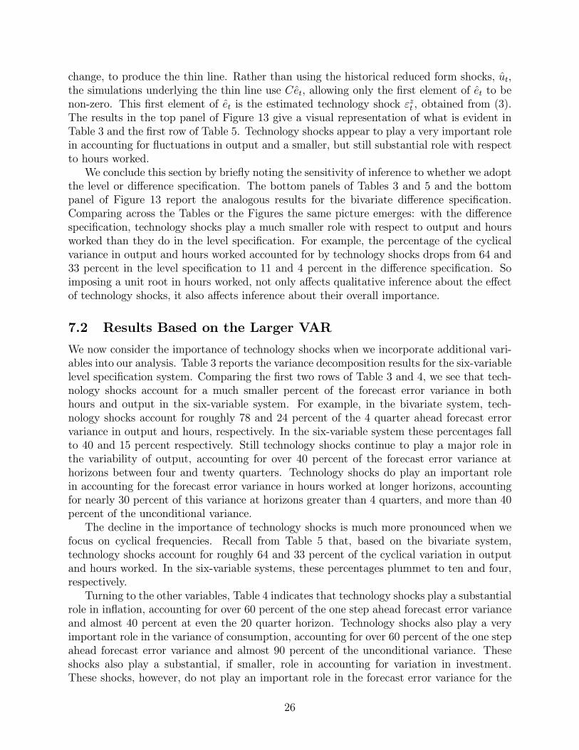
change, to produce the thin line. Rather than using the historical reduced form shocks, ut,the simulations underlying the thin line use Cet, allowing only the first element of et to benon-zero. This first element of et is the estimated technology shock εzt , obtained from (3).The results in the top panel of Figure 13 give a visual representation of what is evident inTable 3 and the first row of Table 5. Technology shocks appear to play a very important rolein accounting for fluctuations in output and a smaller, but still substantial role with respectto hours worked.We conclude this section by briefly noting the sensitivity of inference to whether we adopt

the level or difference specification. The bottom panels of Tables 3 and 5 and the bottompanel of Figure 13 report the analogous results for the bivariate difference specification.Comparing across the Tables or the Figures the same picture emerges: with the differencespecification, technology shocks play a much smaller role with respect to output and hoursworked than they do in the level specification. For example, the percentage of the cyclicalvariance in output and hours worked accounted for by technology shocks drops from 64 and33 percent in the level specification to 11 and 4 percent in the difference specification. Soimposing a unit root in hours worked, not only affects qualitative inference about the effectof technology shocks, it also affects inference about their overall importance.

7.2 Results Based on the Larger VAR

We now consider the importance of technology shocks when we incorporate additional vari-ables into our analysis. Table 3 reports the variance decomposition results for the six-variablelevel specification system. Comparing the first two rows of Table 3 and 4, we see that tech-nology shocks account for a much smaller percent of the forecast error variance in bothhours and output in the six-variable system. For example, in the bivariate system, tech-nology shocks account for roughly 78 and 24 percent of the 4 quarter ahead forecast errorvariance in output and hours, respectively. In the six-variable system these percentages fallto 40 and 15 percent respectively. Still technology shocks continue to play a major role inthe variability of output, accounting for over 40 percent of the forecast error variance athorizons between four and twenty quarters. Technology shocks do play an important rolein accounting for the forecast error variance in hours worked at longer horizons, accountingfor nearly 30 percent of this variance at horizons greater than 4 quarters, and more than 40percent of the unconditional variance.The decline in the importance of technology shocks is much more pronounced when we

focus on cyclical frequencies. Recall from Table 5 that, based on the bivariate system,technology shocks account for roughly 64 and 33 percent of the cyclical variation in outputand hours worked. In the six-variable systems, these percentages plummet to ten and four,respectively.Turning to the other variables, Table 4 indicates that technology shocks play a substantial

role in inflation, accounting for over 60 percent of the one step ahead forecast error varianceand almost 40 percent at even the 20 quarter horizon. Technology shocks also play a veryimportant role in the variance of consumption, accounting for over 60 percent of the one stepahead forecast error variance and almost 90 percent of the unconditional variance. Theseshocks also play a substantial, if smaller, role in accounting for variation in investment.These shocks, however, do not play an important role in the forecast error variance for the

26

federal funds rate.Turning to business cycle frequencies, two results stand out in Table 5. First, technol-

ogy shocks account for a very small percentage of the cyclical variance in output, hoursworked, investment and the federal funds rate (10, 4, 1 and 7 percent respectively). Second,technology shocks account for a moderately large percentage of the cyclical variation in con-sumption (16.7 percent) and a surprisingly large amount of the cyclical variation in inflation(32 percent).Figure 14 presents the historical decompositions for the six-variable level specification

VAR. Technology shocks do relatively well at accounting for the data on output, hours,consumption, inflation and to some extent investment at the lower frequencies. While notreported here, the results are similar for the six-variable difference specification VAR.

8 Conclusions

A theme of this paper is that the treatment of the low frequency component of per capitahours worked has an important impact on inference about the response of hours worked toa technology shock. We explored the impact on inference of treating per capita hours asdifference stationary, stationary, or stationary about a deterministic trend. We concludethat the evidence overwhelmingly favors specifications which imply that per capita hoursworked rises in response to a technology shock.Throughout, we assume that only one shock affects productivity in the long run and

we refer to it as a ‘technology shock’. We do this because it is the standard interpretationin the literature. But, other interpretations are possible. For example, the shock that weidentify could in principle be any permanent disturbance that affects the rate of returnon capital, such as the capital tax rate, the depreciation rate, or agents’ discount rate.If some or all of these shocks are operative and have permanent effects on productivity,then our inferences may be distorted. To explore this possibility requires making additionalidentifying assumptions and incorporating new data into the analysis. Fisher (2002) does thisby considering two types of technology shocks. He argues that investment-specific shocksplay a relatively important role at cyclical frequencies in driving aggregate fluctuations.Significantly, he finds that our key result is robust to the presence of a second shock: bothof the technology shocks that Fisher identifies lead to an increase in hours worked.

27

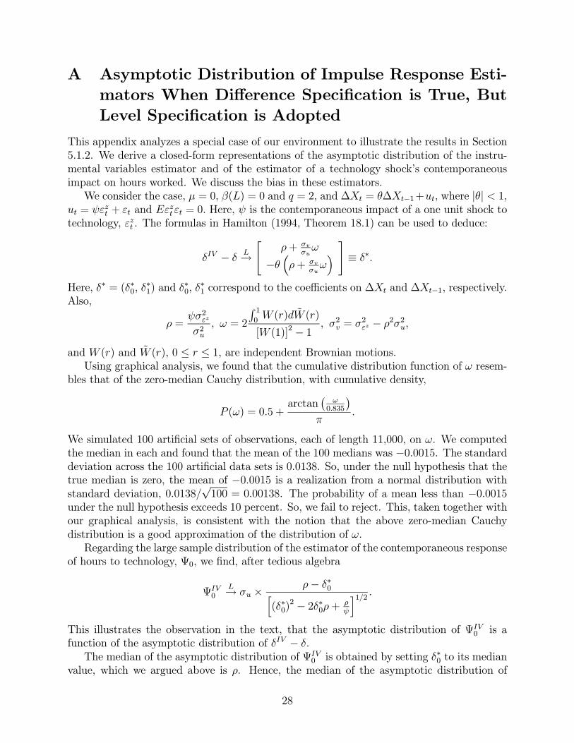
A Asymptotic Distribution of Impulse Response Esti-

mators When Difference Specification is True, But

Level Specification is Adopted

This appendix analyzes a special case of our environment to illustrate the results in Section5.1.2. We derive a closed-form representations of the asymptotic distribution of the instru-mental variables estimator and of the estimator of a technology shock’s contemporaneousimpact on hours worked. We discuss the bias in these estimators.We consider the case, µ = 0, β(L) = 0 and q = 2, and ∆Xt = θ∆Xt−1+ut, where |θ| < 1,

ut = ψεzt + εt and Eεzt εt = 0. Here, ψ is the contemporaneous impact of a one unit shock to

technology, εzt . The formulas in Hamilton (1994, Theorem 18.1) can be used to deduce:

δIV − δL→"

ρ+ σvσuω

−θ³ρ+ σv

σuω´ # ≡ δ∗.

Here, δ∗ = (δ∗0, δ∗1) and δ∗0, δ

∗1 correspond to the coefficients on ∆Xt and ∆Xt−1, respectively.

Also,

ρ =ψσ2εz

σ2u, ω = 2

R 10W (r)dW (r)

[W (1)]2 − 1 , σ2v = σ2εz − ρ2σ2u,

and W (r) and W (r), 0 ≤ r ≤ 1, are independent Brownian motions.Using graphical analysis, we found that the cumulative distribution function of ω resem-

bles that of the zero-median Cauchy distribution, with cumulative density,

P (ω) = 0.5 +arctan

¡ω

0.835

¢π

.

We simulated 100 artificial sets of observations, each of length 11,000, on ω. We computedthe median in each and found that the mean of the 100 medians was −0.0015. The standarddeviation across the 100 artificial data sets is 0.0138. So, under the null hypothesis that thetrue median is zero, the mean of −0.0015 is a realization from a normal distribution withstandard deviation, 0.0138/

√100 = 0.00138. The probability of a mean less than −0.0015

under the null hypothesis exceeds 10 percent. So, we fail to reject. This, taken together withour graphical analysis, is consistent with the notion that the above zero-median Cauchydistribution is a good approximation of the distribution of ω.Regarding the large sample distribution of the estimator of the contemporaneous response

of hours to technology, Ψ0, we find, after tedious algebra

ΨIV0

L→ σu × ρ− δ∗0h(δ∗0)

2 − 2δ∗0ρ+ ρψ

i1/2 .This illustrates the observation in the text, that the asymptotic distribution of ΨIV

0 is afunction of the asymptotic distribution of δIV − δ.The median of the asymptotic distribution of ΨIV0 is obtained by setting δ∗0 to its median

value, which we argued above is ρ. Hence, the median of the asymptotic distribution of

28

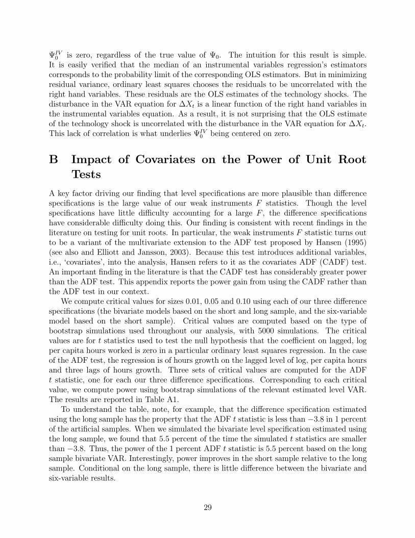
ΨIV0 is zero, regardless of the true value of Ψ0. The intuition for this result is simple.

It is easily verified that the median of an instrumental variables regression’s estimatorscorresponds to the probability limit of the corresponding OLS estimators. But in minimizingresidual variance, ordinary least squares chooses the residuals to be uncorrelated with theright hand variables. These residuals are the OLS estimates of the technology shocks. Thedisturbance in the VAR equation for ∆Xt is a linear function of the right hand variables inthe instrumental variables equation. As a result, it is not surprising that the OLS estimateof the technology shock is uncorrelated with the disturbance in the VAR equation for ∆Xt.This lack of correlation is what underlies ΨIV

0 being centered on zero.

B Impact of Covariates on the Power of Unit Root

Tests

A key factor driving our finding that level specifications are more plausible than differencespecifications is the large value of our weak instruments F statistics. Though the levelspecifications have little difficulty accounting for a large F , the difference specificationshave considerable difficulty doing this. Our finding is consistent with recent findings in theliterature on testing for unit roots. In particular, the weak instruments F statistic turns outto be a variant of the multivariate extension to the ADF test proposed by Hansen (1995)(see also and Elliott and Jansson, 2003). Because this test introduces additional variables,i.e., ‘covariates’, into the analysis, Hansen refers to it as the covariates ADF (CADF) test.An important finding in the literature is that the CADF test has considerably greater powerthan the ADF test. This appendix reports the power gain from using the CADF rather thanthe ADF test in our context.We compute critical values for sizes 0.01, 0.05 and 0.10 using each of our three difference

specifications (the bivariate models based on the short and long sample, and the six-variablemodel based on the short sample). Critical values are computed based on the type ofbootstrap simulations used throughout our analysis, with 5000 simulations. The criticalvalues are for t statistics used to test the null hypothesis that the coefficient on lagged, logper capita hours worked is zero in a particular ordinary least squares regression. In the caseof the ADF test, the regression is of hours growth on the lagged level of log, per capita hoursand three lags of hours growth. Three sets of critical values are computed for the ADFt statistic, one for each our three difference specifications. Corresponding to each criticalvalue, we compute power using bootstrap simulations of the relevant estimated level VAR.The results are reported in Table A1.To understand the table, note, for example, that the difference specification estimated

using the long sample has the property that the ADF t statistic is less than −3.8 in 1 percentof the artificial samples. When we simulated the bivariate level specification estimated usingthe long sample, we found that 5.5 percent of the time the simulated t statistics are smallerthan −3.8. Thus, the power of the 1 percent ADF t statistic is 5.5 percent based on the longsample bivariate VAR. Interestingly, power improves in the short sample relative to the longsample. Conditional on the long sample, there is little difference between the bivariate andsix-variable results.

29

We turn now to an assessment of the impact on power of adding covariates. Our CADF tstatistic resembles the ADF t statistic, except that the underlying regression also includes allthe predetermined variables in the instrumental variables regression, (3). Since the numberof predetermined variables is different in the bivariate and six-variable systems, we have twoCADF t statistics. The first corresponds to our bivariate analysis. It is based on a regressionlike the one underlying the ADF test, except that it also includes four lags of productivitygrowth. The second corresponds to our six-variable analysis. In particular, it adds fourlags of each of the federal funds rate, the rate of inflation, the log of the ratio of nominalconsumption expenditures to nominal GDP, and the log of the ratio of nominal investmentexpenditures to nominal GDP.We compute critical values for our two CADF t statistics in the same way as for the ADF

statistic. In particular, we compute two sets of critical values for our bivariate CADF statis-tic, one corresponding to each of the short and long sample estimated difference specifications.The critical values for the six-variable CADF t statistic are based on bootstrap simulations ofthe estimated six-variable difference VAR. Corresponding to each critical value, we computepower using bootstrap simulations of the relevant estimated level difference VAR.Corresponding to each critical value, we also computed the power of the statistic when

the level specification is true. This was done by bootstrap simulation of the relevant levelspecification VAR. Results are reported in Table A2. Comparing Tables A1 and A2, powerincreases substantially with the introduction of covariates. With a 1 percent size, powerjumps by an order of magnitude in the short sample.

30

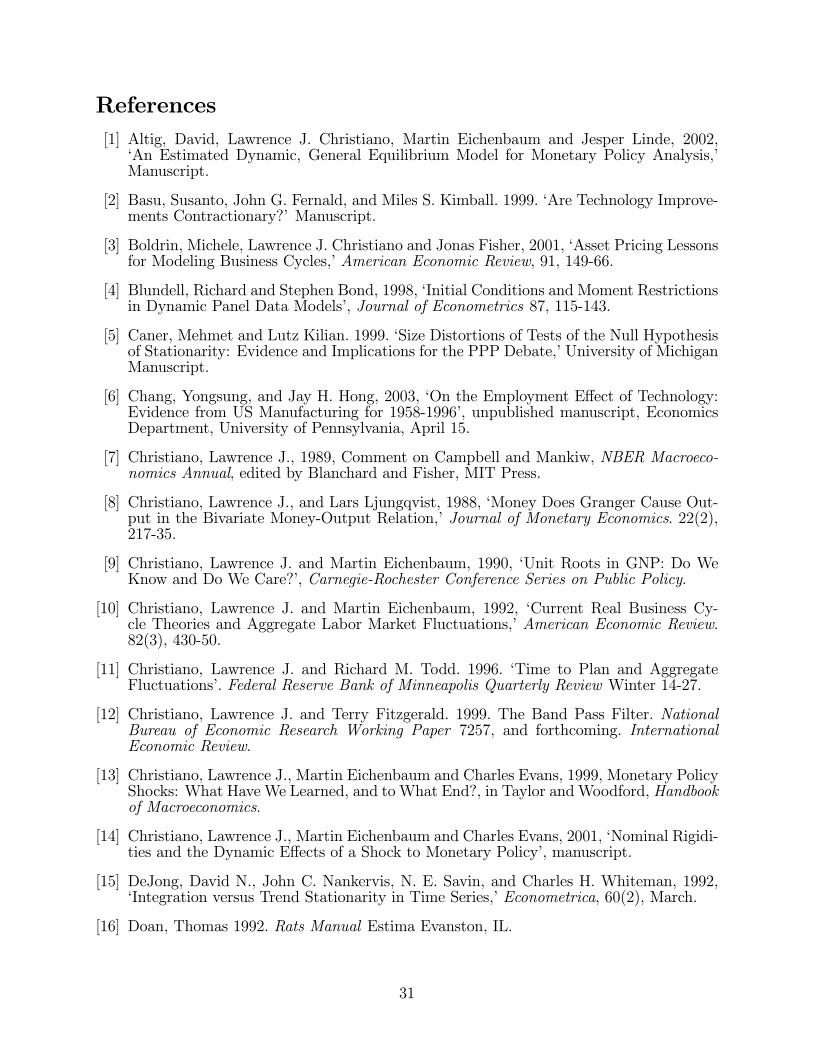
References

[1] Altig, David, Lawrence J. Christiano, Martin Eichenbaum and Jesper Linde, 2002,‘An Estimated Dynamic, General Equilibrium Model for Monetary Policy Analysis,’Manuscript.

[2] Basu, Susanto, John G. Fernald, and Miles S. Kimball. 1999. ‘Are Technology Improve-ments Contractionary?’ Manuscript.

[3] Boldrin, Michele, Lawrence J. Christiano and Jonas Fisher, 2001, ‘Asset Pricing Lessonsfor Modeling Business Cycles,’ American Economic Review, 91, 149-66.

[4] Blundell, Richard and Stephen Bond, 1998, ‘Initial Conditions and Moment Restrictionsin Dynamic Panel Data Models’, Journal of Econometrics 87, 115-143.

[5] Caner, Mehmet and Lutz Kilian. 1999. ‘Size Distortions of Tests of the Null Hypothesisof Stationarity: Evidence and Implications for the PPP Debate,’ University of MichiganManuscript.

[6] Chang, Yongsung, and Jay H. Hong, 2003, ‘On the Employment Effect of Technology:Evidence from US Manufacturing for 1958-1996’, unpublished manuscript, EconomicsDepartment, University of Pennsylvania, April 15.

[7] Christiano, Lawrence J., 1989, Comment on Campbell and Mankiw, NBER Macroeco-nomics Annual, edited by Blanchard and Fisher, MIT Press.

[8] Christiano, Lawrence J., and Lars Ljungqvist, 1988, ‘Money Does Granger Cause Out-put in the Bivariate Money-Output Relation,’ Journal of Monetary Economics. 22(2),217-35.

[9] Christiano, Lawrence J. and Martin Eichenbaum, 1990, ‘Unit Roots in GNP: Do WeKnow and Do We Care?’, Carnegie-Rochester Conference Series on Public Policy.

[10] Christiano, Lawrence J. and Martin Eichenbaum, 1992, ‘Current Real Business Cy-cle Theories and Aggregate Labor Market Fluctuations,’ American Economic Review.82(3), 430-50.

[11] Christiano, Lawrence J. and Richard M. Todd. 1996. ‘Time to Plan and AggregateFluctuations’. Federal Reserve Bank of Minneapolis Quarterly Review Winter 14-27.

[12] Christiano, Lawrence J. and Terry Fitzgerald. 1999. The Band Pass Filter. NationalBureau of Economic Research Working Paper 7257, and forthcoming. InternationalEconomic Review.

[13] Christiano, Lawrence J., Martin Eichenbaum and Charles Evans, 1999, Monetary PolicyShocks: What Have We Learned, and to What End?, in Taylor andWoodford, Handbookof Macroeconomics.

[14] Christiano, Lawrence J., Martin Eichenbaum and Charles Evans, 2001, ‘Nominal Rigidi-ties and the Dynamic Effects of a Shock to Monetary Policy’, manuscript.

[15] DeJong, David N., John C. Nankervis, N. E. Savin, and Charles H. Whiteman, 1992,‘Integration versus Trend Stationarity in Time Series,’ Econometrica, 60(2), March.

[16] Doan, Thomas 1992. Rats Manual Estima Evanston, IL.

31

[17] Eichenbaum, Martin, and Kenneth J. Singleton 1986. ‘Do Equilibrium Real BusinessCycle Theories Explain Postwar U.S Business Cycles?’ NBER Macroeconomics Annual1986, 91-135.

[18] Elliott, Graham, and Michael Jansson, 2003, ‘Testing for Unit Roots with StationaryCovariates,’ Journal of Econometrics, 115, 75-89.

[19] Fisher, Jonas, 2002, ‘Technology Shocks Matter,’ Federal Reserve Bank of ChicagoWorking Paper 2002-14

[20] Francis, Neville, and Valerie A. Ramey, 2003, ‘Is the Technology-Driven Real BusinessCycle Hypothesis Dead? Shocks and Aggregate Fluctuations Revisited,’ manuscript,UCSD.

[21] Gali, Jordi, 1999, ‘Technology, Employment, and the Business Cycle: Do TechnologyShocks Explain Aggregate Fluctuations?’ American Economic Review, 89(1), 249-271.

[22] Gali, Jordi, Mark Gertler and J. David Lopez-Salido, 2001, ‘Markups, Gaps and theWelfare Costs of Business Fluctuations,’ May.

[23] Gali, Jordi, J. David Lopez-Salido, and Javier Valles, 2002, ‘Technology Shocks andMonetary Policy: Assessing the Fed’s Performance’, National Bureau of Economic Re-search Working Paper 8768.

[24] Gali, Jordi and Pau Rabanal, 2004. ‘Technology Shocks and Aggregate Fluctuations:How Well Does the RBC Model Fit Postwar U.S. Data?’, forthcoming, NBER Macroe-conomics Annual.

[25] Hahn, Jinyong, Jerry Hausman and Guido Kuersteiner, 2001, ‘Bias Corrected Instru-mental Variables Estimation for Dynamic Panel Models with Fixed Effects,’ manuscript,MIT.

[26] Hansen, Bruce E., 1995, ‘Rethinking the Univariate Approach to Unit Root Testing:Using Covariates to Increase Power,’ Econometric Theory, December,11(5),1148-71

[27] Hamilton, James B., 1994, Time Series Analysis, Princeton University Press, PrincetonNew Jersey.

[28] Kwiatkowski, D., Phillips, P.C.B., Schmidt, P., and Shin, Y. 1992, ‘Testing the NullHypothesis of Stationarity Against the Alternative of a Unit Root,’ Journal of Econo-metrics, 54, 159-178.

[29] King, Robert, Charles Plosser, James Stock and Mark Watson, 1991, ‘Stochastic Trendsand Economic Fluctuations,’ American Economic Review, 81, 819-840.

[30] Leybourne, Stephen J. and B.P.M. McCabe, 1994, ‘A Consistent Test for a Unit Root’,Journal of Business and Economic Statistics, 12(2), 157-66

[31] Shapiro, Matthew, and Mark Watson, 1988, ‘Sources of Business Cycle Fluctuations,’NBER,Macroeconomics Annual, 111-148.

[32] Shea, John 1998. ‘What Do Technology Shocks Do?,’ National Bureau of EconomicResearch Working Papers 6632

[33] Sims, Christopher, James Stock and Mark Watson, 1990. ‘Inference in Linear TimeSeries Models with Some Unit Roots,’ Econometrica 58(1), 113-144.

32

[34] Staiger, Douglas, and James Stock, 1997, ‘Instrumental Variables Regression with WeakInstruments,’ Econometrica, 65(3), 557-586.

[35] Uhlig, Harald (2004). ‘Do Technology Shocks Lead to a Fall in Total Hours Worked?’,forthcoming, Journal of the European Economic Association.

[36] Vigfusson, Robert J. 2004, ‘The Delayed Response to A Technology Shock: A FlexiblePrice Explanation’ Federal Reserve Board International Finance Discussion Paper 810.

33

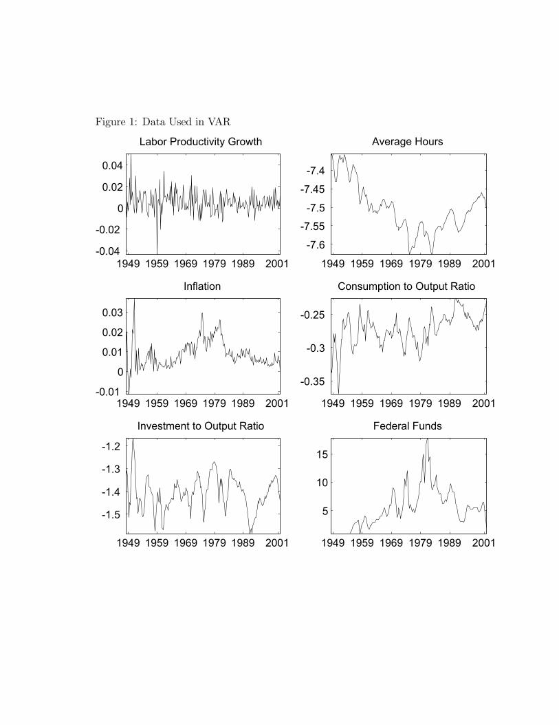
Figure 1: Data Used in VAR

1949 1959 1969 1979 1989 2001-0.04

-0.02

0

0.02

0.04

Labor Productivity Growth

1949 1959 1969 1979 1989 2001

-7.6

-7.55

-7.5

-7.45

-7.4

Average Hours

1949 1959 1969 1979 1989 2001-0.01

0

0.01

0.02

0.03

Inflation

1949 1959 1969 1979 1989 2001

-0.35

-0.3

-0.25

Consumption to Output Ratio

1949 1959 1969 1979 1989 2001

-1.5

-1.4

-1.3

-1.2

Investment to Output Ratio

1949 1959 1969 1979 1989 2001

5

10

15

Federal Funds

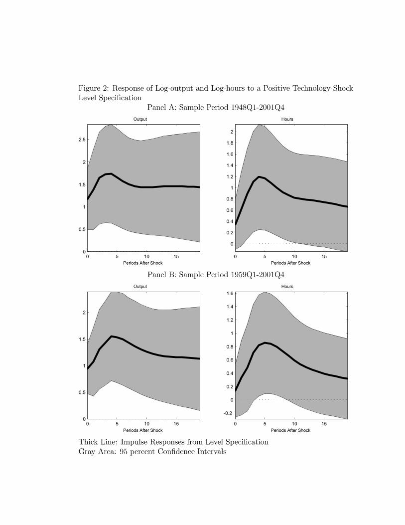
Figure 2: Response of Log-output and Log-hours to a Positive Technology ShockLevel Specification

Panel A: Sample Period 1948Q1-2001Q4

0 5 10 150

0.5

1

1.5

2

2.5

Output

Periods After Shock0 5 10 15

0

0.2

0.4

0.6

0.8

1

1.2

1.4

1.6

1.8

2

Hours

Periods After Shock

Panel B: Sample Period 1959Q1-2001Q4

0 5 10 150

0.5

1

1.5

2

Output

Periods After Shock0 5 10 15

-0.2

0

0.2

0.4

0.6

0.8

1

1.2

1.4

1.6Hours

Periods After Shock

Thick Line: Impulse Responses from Level SpecificationGray Area: 95 percent Confidence Intervals

Figure 3: Response of Log-output and Log-hours to a Positive Technology ShockDifference Specification

Panel A: Sample Period 1948Q1-2001Q4

0 5 10 150

0.5

1

1.5

Output

Periods After Shock0 5 10 15

-0.6

-0.4

-0.2

0

0.2

0.4

0.6

Hours

Periods After Shock

Panel B: Sample Period 1959Q1-2001Q4

0 5 10 15

0

0.5

1

1.5

Output

Periods After Shock0 5 10 15

-0.6

-0.4

-0.2

0

0.2

0.4

0.6

0.8Hours

Periods After Shock

Line with Triangles: Impulse Responses from Difference SpecificationGray Area: 95 percent Confidence Intervals

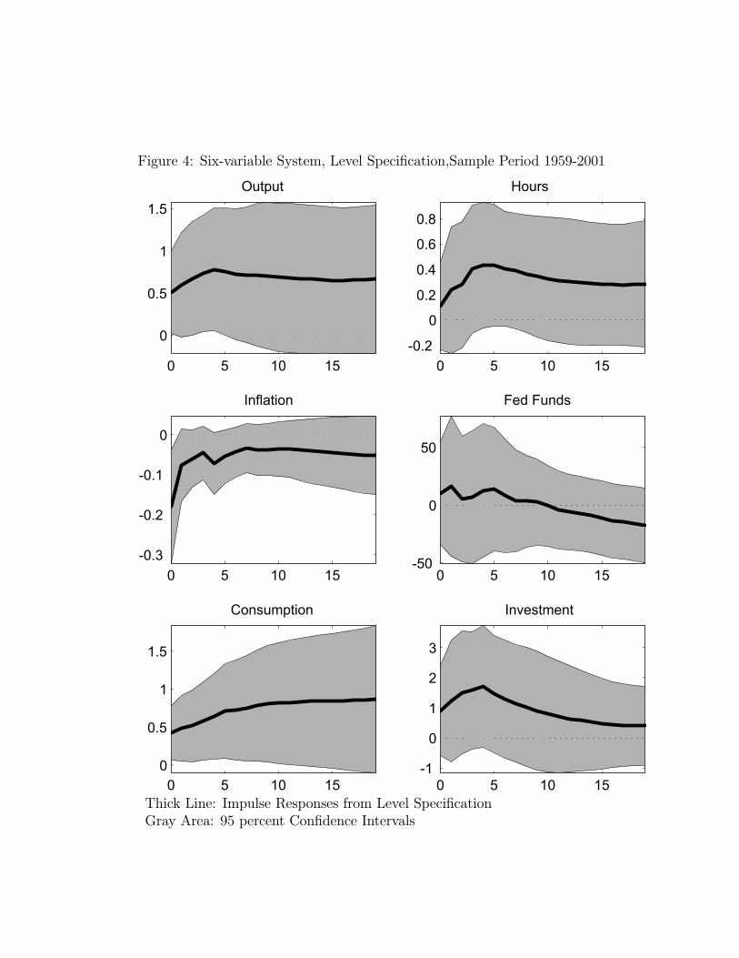
Figure 4: Six-variable System, Level Specification,Sample Period 1959-2001

0 5 10 15

0

0.5

1

1.5Output

0 5 10 15-0.2

0

0.2

0.4

0.6

0.8

Hours

0 5 10 15-0.3

-0.2

-0.1

0

Inflation

0 5 10 15-50

0

50

Fed Funds

0 5 10 150

0.5

1

1.5

Consumption

0 5 10 15-1

0

1

2

3

Investment

Thick Line: Impulse Responses from Level SpecificationGray Area: 95 percent Confidence Intervals

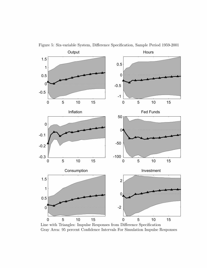
Figure 5: Six-variable System, Difference Specification, Sample Period 1959-2001

0 5 10 15

-0.5

0

0.5

1

1.5

Output

0 5 10 15-1

-0.5

0

0.5

Hours

0 5 10 15-0.3

-0.2

-0.1

0

Inflation

0 5 10 15-100

-50

0

50Fed Funds

0 5 10 15

0

0.5

1

1.5

Consumption

0 5 10 15

-2

0

2

Investment

Line with Triangles: Impulse Responses from Difference SpecificationGray Area: 95 percent Confidence Intervals For Simulation Impulse Responses

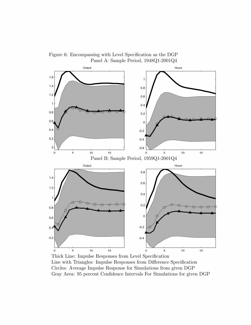
Figure 6: Encompassing with Level Specification as the DGPPanel A: Sample Period, 1948Q1-2001Q4

0 5 10 15

0

0.2

0.4

0.6

0.8

1

1.2

1.4

1.6

Output

0 5 10 15-0.6

-0.4

-0.2

0

0.2

0.4

0.6

0.8

1

Hours

Panel B: Sample Period, 1959Q1-2001Q4

0 5 10 15

0.2

0.4

0.6

0.8

1

1.2

1.4

Output

0 5 10 15

-0.4

-0.2

0

0.2

0.4

0.6

0.8

Hours

Thick Line: Impulse Responses from Level SpecificationLine with Triangles: Impulse Responses from Difference SpecificationCircles: Average Impulse Response for Simulations from given DGPGray Area: 95 percent Confidence Intervals For Simulations for given DGP

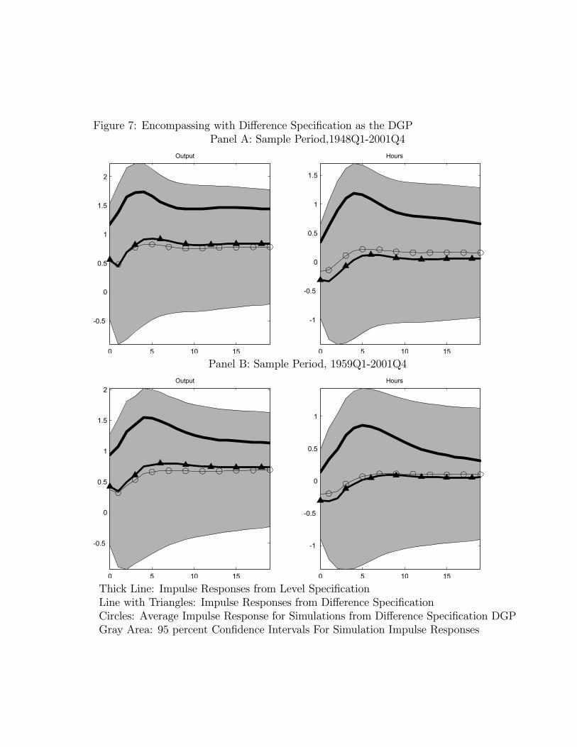
Figure 7: Encompassing with Difference Specification as the DGPPanel A: Sample Period,1948Q1-2001Q4

0 5 10 15

-0.5

0

0.5

1

1.5

2

Output

0 5 10 15

-1

-0.5

0

0.5

1

1.5

Hours

Panel B: Sample Period, 1959Q1-2001Q4

0 5 10 15

-0.5

0

0.5

1

1.5

2Output

0 5 10 15

-1

-0.5

0

0.5

1

Hours

Thick Line: Impulse Responses from Level SpecificationLine with Triangles: Impulse Responses from Difference SpecificationCircles: Average Impulse Response for Simulations from Difference Specification DGPGray Area: 95 percent Confidence Intervals For Simulation Impulse Responses

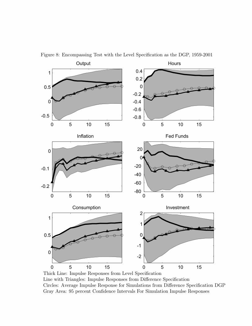
Figure 8: Encompassing Test with the Level Specification as the DGP, 1959-2001

0 5 10 15

-0.5

0

0.5

1

Output

0 5 10 15-0.8-0.6-0.4-0.2

00.20.4

Hours

0 5 10 15

-0.2

-0.1

0

Inflation

0 5 10 15-80

-60

-40

-20

0

20

Fed Funds

0 5 10 15

0

0.5

1

Consumption

0 5 10 15

-2

-1

0

1

2Investment

Thick Line: Impulse Responses from Level SpecificationLine with Triangles: Impulse Responses from Difference SpecificationCircles: Average Impulse Response for Simulations from Difference Specification DGPGray Area: 95 percent Confidence Intervals For Simulation Impulse Responses

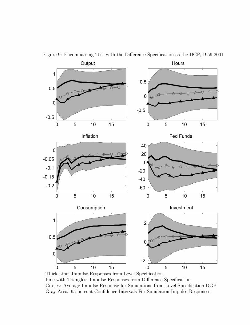
Figure 9: Encompassing Test with the Difference Specification as the DGP, 1959-2001

0 5 10 15-0.5

0

0.5

1

Output

0 5 10 15

-0.5

0

0.5

Hours

0 5 10 15

-0.2

-0.15

-0.1

-0.05

0

Inflation

0 5 10 15

-60

-40

-20

0

20

40

Fed Funds

0 5 10 15

0

0.5

1

Consumption

0 5 10 15-2

0

2

Investment

Thick Line: Impulse Responses from Level SpecificationLine with Triangles: Impulse Responses from Difference SpecificationCircles: Average Impulse Response for Simulations from Level Specification DGPGray Area: 95 percent Confidence Intervals For Simulation Impulse Responses

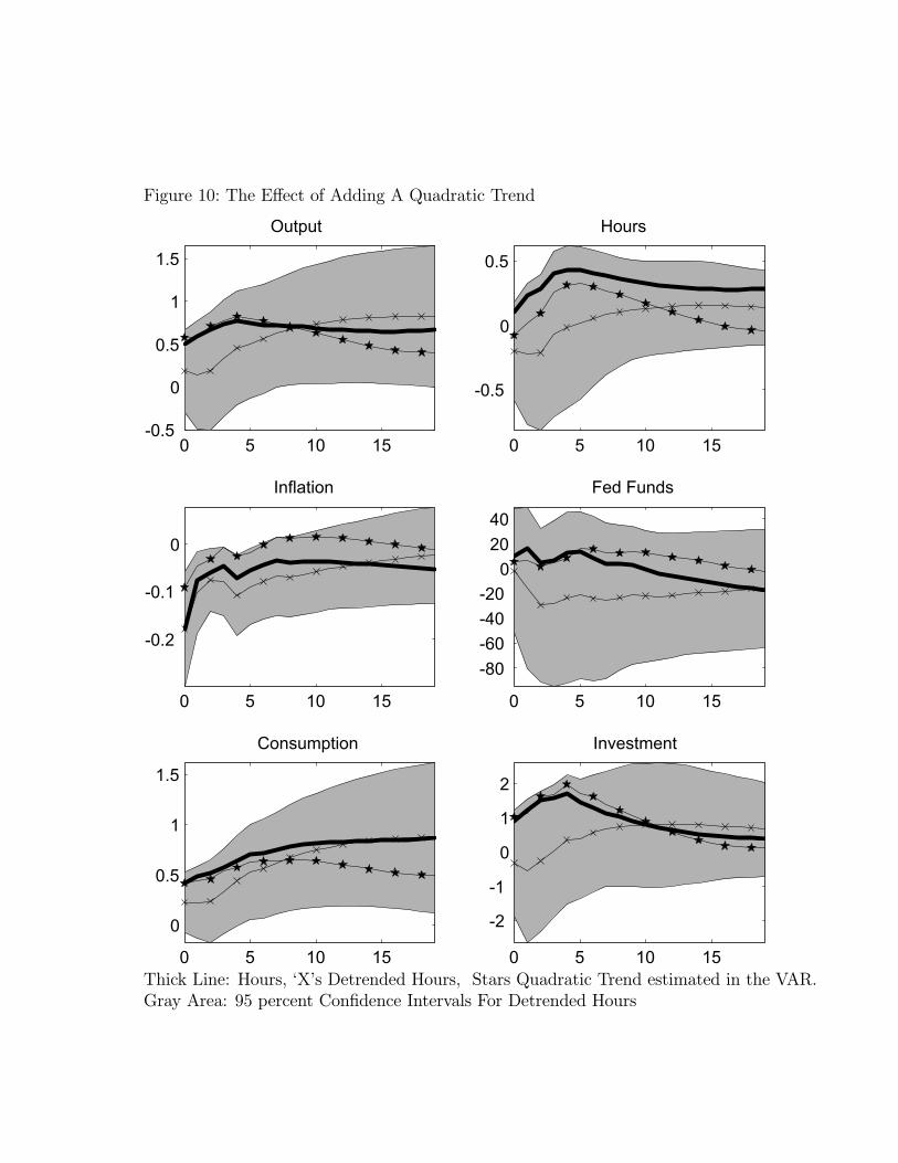
Figure 10: The Effect of Adding A Quadratic Trend

0 5 10 15-0.5

0

0.5

1

1.5

Output

0 5 10 15

-0.5

0

0.5

Hours

0 5 10 15

-0.2

-0.1

0

Inflation

0 5 10 15

-80-60-40-20

02040

Fed Funds

0 5 10 15

0

0.5

1

1.5

Consumption

0 5 10 15

-2

-1

0

1

2

Investment

Thick Line: Hours, ‘X’s Detrended Hours, Stars Quadratic Trend estimated in the VAR.Gray Area: 95 percent Confidence Intervals For Detrended Hours

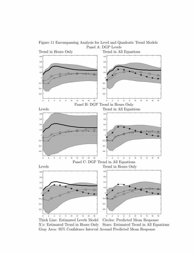
Figure 11 Encompassing Analysis for Level and Quadratic Trend ModelsPanel A: DGP Levels

Trend in Hours Only Trend in All Equations

0 2 4 6 8 10 12 14 16 18

-0.6

-0.4

-0.2

0

0.2

0.4

0.6

0.8

0 2 4 6 8 10 12 14 16 18

-0.6

-0.4

-0.2

0

0.2

0.4

0.6

0.8

Panel B: DGP Trend in Hours OnlyLevels Trend in All Equations

0 2 4 6 8 10 12 14 16 18

-0.6

-0.4

-0.2

0

0.2

0.4

0.6

0.8

0 2 4 6 8 10 12 14 16 18

-0.6

-0.4

-0.2

0

0.2

0.4

0.6

0.8

Panel C: DGP Trend in All EquationsLevels Trend in Hours Only

0 2 4 6 8 10 12 14 16 18

-0.6

-0.4

-0.2

0

0.2

0.4

0.6

0.8

0 2 4 6 8 10 12 14 16 18

-0.6

-0.4

-0.2

0

0.2

0.4

0.6

0.8

Thick Line: Estimated Levels Model Circles: Predicted Mean ResponseX’s: Estimated Trend in Hours Only Stars: Estimated Trend in All EquationsGray Area: 95% Confidence Interval Around Predicted Mean Response

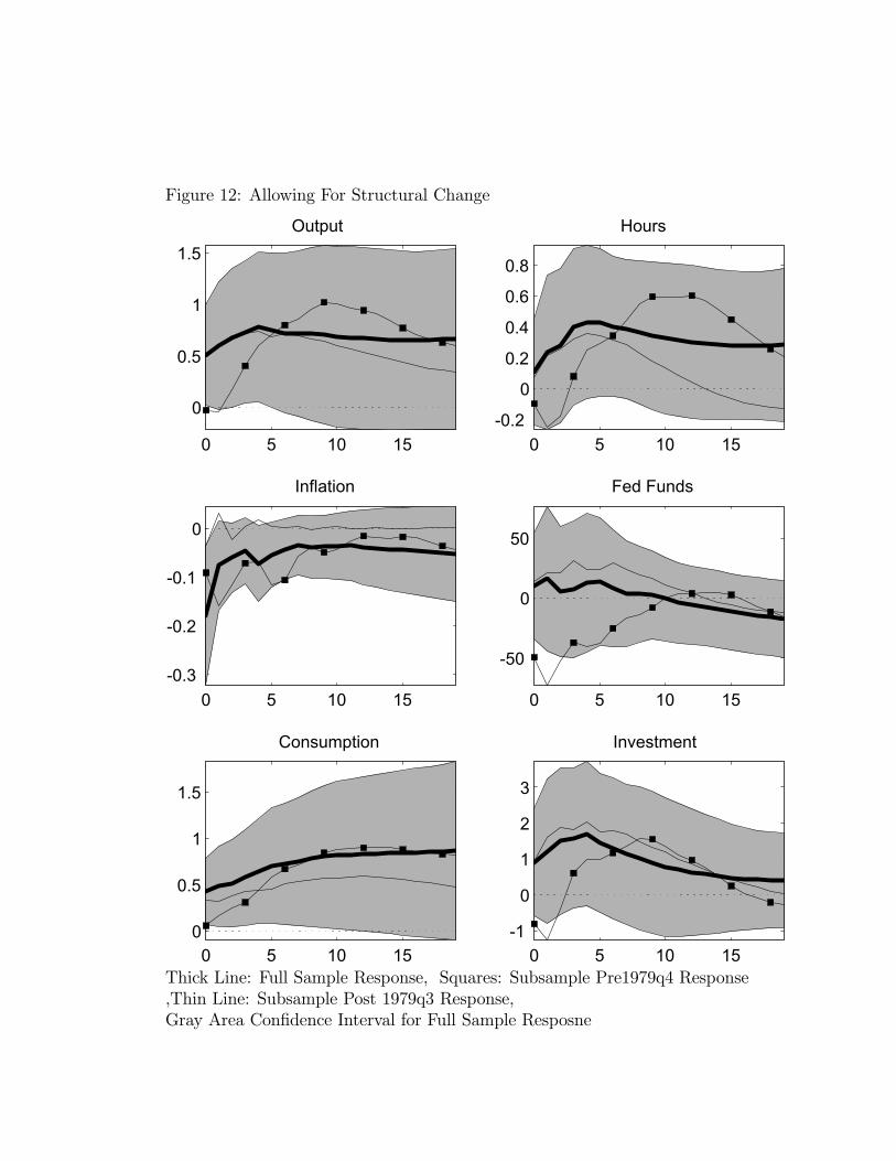
Figure 12: Allowing For Structural Change

0 5 10 15

0

0.5

1

1.5Output

0 5 10 15-0.2

0

0.2

0.4

0.6

0.8

Hours

0 5 10 15-0.3

-0.2

-0.1

0

Inflation

0 5 10 15

-50

0

50

Fed Funds

0 5 10 150

0.5

1

1.5

Consumption

0 5 10 15-1

0

1

2

3

Investment

Thick Line: Full Sample Response, Squares: Subsample Pre1979q4 Response,Thin Line: Subsample Post 1979q3 Response,Gray Area Confidence Interval for Full Sample Resposne

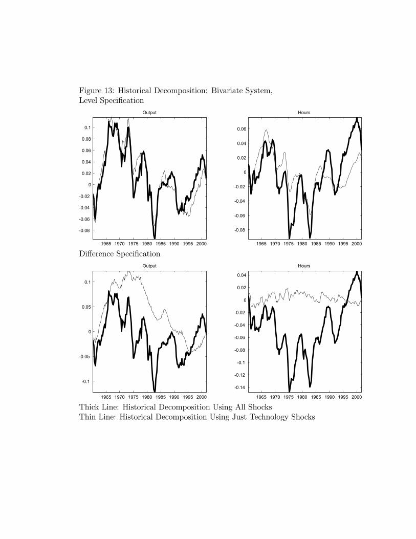
Figure 13: Historical Decomposition: Bivariate System,Level Specification

1965 1970 1975 1980 1985 1990 1995 2000

-0.08

-0.06

-0.04

-0.02

0

0.02

0.04

0.06

0.08

0.1

Output

1965 1970 1975 1980 1985 1990 1995 2000

-0.08

-0.06

-0.04

-0.02

0

0.02

0.04

0.06

Hours

Difference Specification

1965 1970 1975 1980 1985 1990 1995 2000

-0.1

-0.05

0

0.05

0.1

Output

1965 1970 1975 1980 1985 1990 1995 2000

-0.14

-0.12

-0.1

-0.08

-0.06

-0.04

-0.02

0

0.02

0.04

Hours

Thick Line: Historical Decomposition Using All ShocksThin Line: Historical Decomposition Using Just Technology Shocks

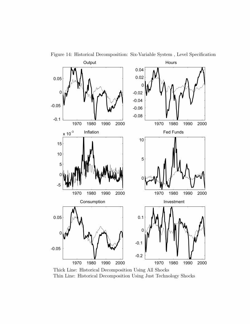
Figure 14: Historical Decomposition: Six-Variable System , Level Specification

1970 1980 1990 2000-0.1

-0.05

0

0.05

Output

1970 1980 1990 2000

-0.08

-0.06

-0.04

-0.02

0

0.02

0.04

Hours

1970 1980 1990 2000

-5

0

5

10

15

x 10-3 Inflation

1970 1980 1990 2000

0

5

10

Fed Funds

1970 1980 1990 2000

-0.05

0

0.05

Consumption

1970 1980 1990 2000

-0.2

-0.1

0

0.1

Investment

Thick Line: Historical Decomposition Using All ShocksThin Line: Historical Decomposition Using Just Technology Shocks

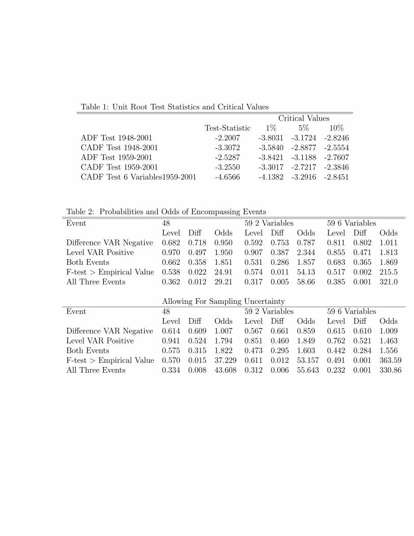
Table 1: Unit Root Test Statistics and Critical Values

Critical ValuesTest-Statistic 1% 5% 10%

ADF Test 1948-2001 -2.2007 -3.8031 -3.1724 -2.8246CADF Test 1948-2001 -3.3072 -3.5840 -2.8877 -2.5554ADF Test 1959-2001 -2.5287 -3.8421 -3.1188 -2.7607CADF Test 1959-2001 -3.2550 -3.3017 -2.7217 -2.3846CADF Test 6 Variables1959-2001 -4.6566 -4.1382 -3.2916 -2.8451

Table 2: Probabilities and Odds of Encompassing Events

Event 48 59 2 Variables 59 6 VariablesLevel Diff Odds Level Diff Odds Level Diff Odds

Difference VAR Negative 0.682 0.718 0.950 0.592 0.753 0.787 0.811 0.802 1.011Level VAR Positive 0.970 0.497 1.950 0.907 0.387 2.344 0.855 0.471 1.813Both Events 0.662 0.358 1.851 0.531 0.286 1.857 0.683 0.365 1.869F-test > Empirical Value 0.538 0.022 24.91 0.574 0.011 54.13 0.517 0.002 215.5All Three Events 0.362 0.012 29.21 0.317 0.005 58.66 0.385 0.001 321.0

Allowing For Sampling UncertaintyEvent 48 59 2 Variables 59 6 Variables

Level Diff Odds Level Diff Odds Level Diff OddsDifference VAR Negative 0.614 0.609 1.007 0.567 0.661 0.859 0.615 0.610 1.009Level VAR Positive 0.941 0.524 1.794 0.851 0.460 1.849 0.762 0.521 1.463Both Events 0.575 0.315 1.822 0.473 0.295 1.603 0.442 0.284 1.556F-test > Empirical Value 0.570 0.015 37.229 0.611 0.012 53.157 0.491 0.001 363.59All Three Events 0.334 0.008 43.608 0.312 0.006 55.643 0.232 0.001 330.86

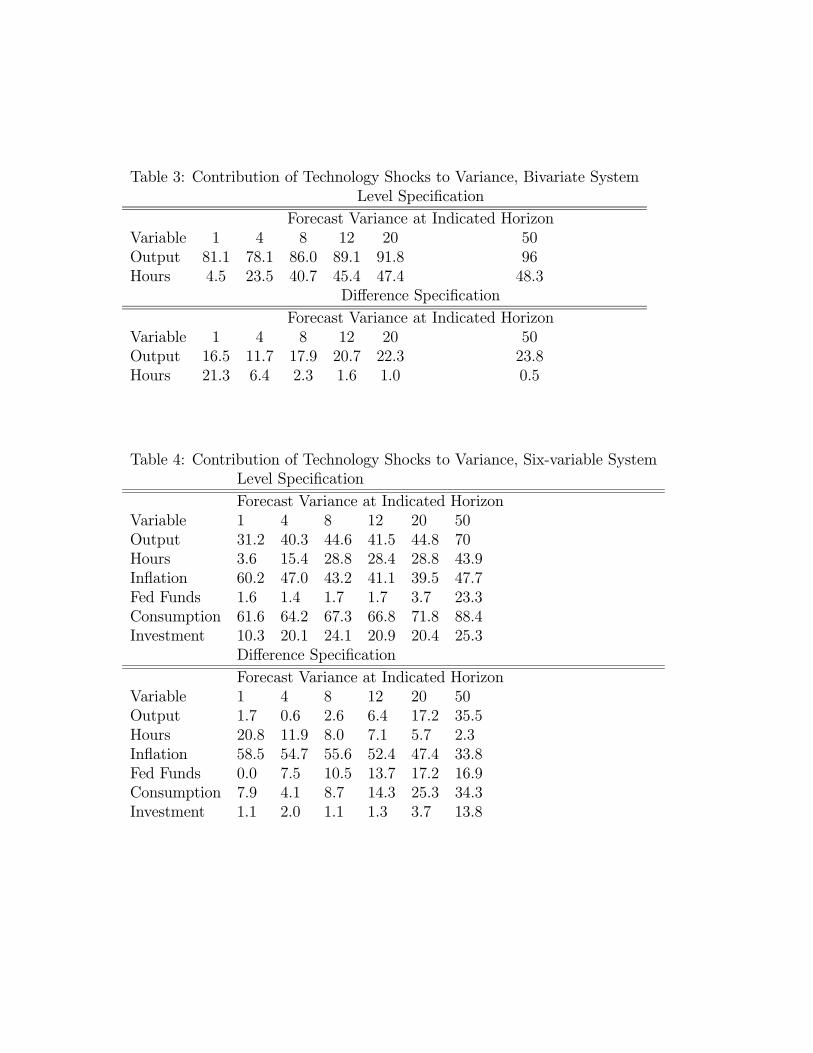
Table 3: Contribution of Technology Shocks to Variance, Bivariate SystemLevel Specification

Forecast Variance at Indicated HorizonVariable 1 4 8 12 20 50Output 81.1 78.1 86.0 89.1 91.8 96Hours 4.5 23.5 40.7 45.4 47.4 48.3

Difference Specification

Forecast Variance at Indicated HorizonVariable 1 4 8 12 20 50Output 16.5 11.7 17.9 20.7 22.3 23.8Hours 21.3 6.4 2.3 1.6 1.0 0.5

Table 4: Contribution of Technology Shocks to Variance, Six-variable SystemLevel Specification

Forecast Variance at Indicated HorizonVariable 1 4 8 12 20 50Output 31.2 40.3 44.6 41.5 44.8 70Hours 3.6 15.4 28.8 28.4 28.8 43.9Inflation 60.2 47.0 43.2 41.1 39.5 47.7Fed Funds 1.6 1.4 1.7 1.7 3.7 23.3Consumption 61.6 64.2 67.3 66.8 71.8 88.4Investment 10.3 20.1 24.1 20.9 20.4 25.3

Difference Specification

Forecast Variance at Indicated HorizonVariable 1 4 8 12 20 50Output 1.7 0.6 2.6 6.4 17.2 35.5Hours 20.8 11.9 8.0 7.1 5.7 2.3Inflation 58.5 54.7 55.6 52.4 47.4 33.8Fed Funds 0.0 7.5 10.5 13.7 17.2 16.9Consumption 7.9 4.1 8.7 14.3 25.3 34.3Investment 1.1 2.0 1.1 1.3 3.7 13.8

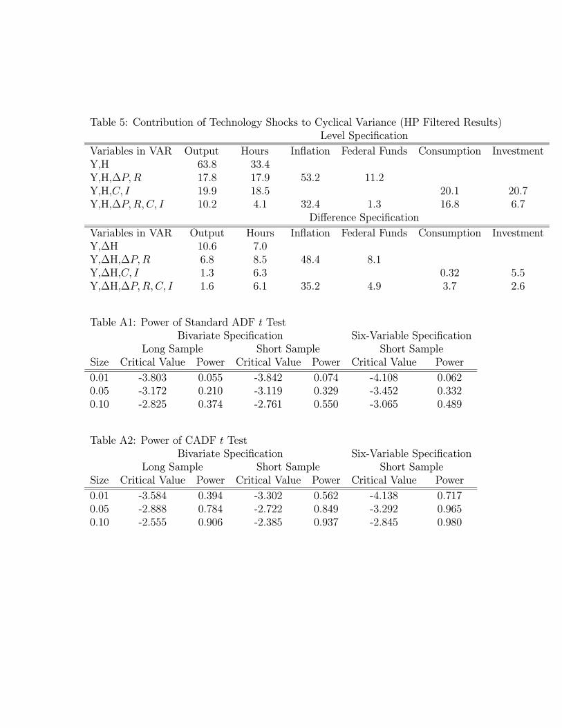
Table 5: Contribution of Technology Shocks to Cyclical Variance (HP Filtered Results)Level Specification

Variables in VAR Output Hours Inflation Federal Funds Consumption InvestmentY,H 63.8 33.4Y,H,∆P,R 17.8 17.9 53.2 11.2Y,H,C, I 19.9 18.5 20.1 20.7Y,H,∆P,R,C, I 10.2 4.1 32.4 1.3 16.8 6.7

Difference Specification

Variables in VAR Output Hours Inflation Federal Funds Consumption InvestmentY,∆H 10.6 7.0Y,∆H,∆P,R 6.8 8.5 48.4 8.1Y,∆H,C, I 1.3 6.3 0.32 5.5Y,∆H,∆P,R,C, I 1.6 6.1 35.2 4.9 3.7 2.6

Table A1: Power of Standard ADF t TestBivariate Specification Six-Variable Specification

Long Sample Short Sample Short SampleSize Critical Value Power Critical Value Power Critical Value Power

0.01 -3.803 0.055 -3.842 0.074 -4.108 0.0620.05 -3.172 0.210 -3.119 0.329 -3.452 0.3320.10 -2.825 0.374 -2.761 0.550 -3.065 0.489

Table A2: Power of CADF t TestBivariate Specification Six-Variable Specification

Long Sample Short Sample Short SampleSize Critical Value Power Critical Value Power Critical Value Power

0.01 -3.584 0.394 -3.302 0.562 -4.138 0.7170.05 -2.888 0.784 -2.722 0.849 -3.292 0.9650.10 -2.555 0.906 -2.385 0.937 -2.845 0.980