WhatHappenedtothe'GreatAmericanJobsMachine'?

MatteoRichiardi,BrianNolanandLaneKenworthy

April18,2019

INETOxfordWorkingPaperNo.2019-04

Employment,Equity&GrowthProgramme

2

What Happened to the 'Great American Jobs Machine'?*

Matteo Richiardi,a,d,e Brian Nolan,b,d and Lane Kenworthyc

aUniversity of Essex

bUniversity of Oxford cUniversity of California-San Diego

d Institute for New Economic Thinking at the Oxford Martin School eCollegio Carlo Alberto

April 18, 2019

* We gratefully acknowledge valuable advice and input from Sylvia Allegretto (Berkeley),

very helpful advice from Bent Nielsen and Steve Bond (Oxford and Nuffield), and funding

from Arrowgrass Capital (London).

3

What Happened to the 'Great American Jobs Machine'?

Abstract

In the 1980s and 1990s the US employment rate increased steadily, and by 2000 it was one of

the highest among the rich democratic nations. Since then it has declined both in absolute

terms and relative to other countries. We use an in-depth comparison between the United

States and the United Kingdom to probe the causes of America's poor recent performance.

Contrary to a common narrative, a comparative perspective suggests that the decline in US

labour force participation is not confined to the (white) male population; the divergence in the

female participation rate is even more pronounced. We do not find evidence that the poor US

performance is linked to cyclical patterns, such as the 2008-09 Great Recession; instead, it is

a more pervasive, longer-run phenomenon. The relative decline of US participation rates

compared to the UK is attributable to shifts in socio-demographic characteristics, such as

education, and to shifts in the impact of those characteristics, which have become more

adverse to participation.

Keywords: Labour force participation, employment, human capital, gender

4

What Happened to the 'Great American Jobs Machine'?

1. Introduction

Labour force participation in the United States increased steadily in the 1980s and 1990s.

However, it declined between 2000 and 2007 and then fell even more sharply in the Great

Recession. Macroeconomic recovery saw unemployment fall rapidly from 2011, but the

participation rate has only increased modestly, remaining well below its pre-crisis level and

even further below its late-1990s peak. An expanding research literature has advanced a

range of explanations for this dramatic reversal in what not long ago was known as the 'great

American jobs machine' (The Economist 2000).

The US experience since 2000 contrasts sharply with what has happened in the United

Kingdom. There, labour force participation was fairly stable in the decade up to the onset of

the Great Recession, fell by much less during the crisis, and since 2012 has been rising

significantly. These two countries have many features in common, including deregulated

labour markets and independent currencies. And both had a comparatively high participation

rate at the end of the 1990s. Given the divergence in participation rates since 2000 and

through the crisis and recovery periods, comparison of these two cases can provide a helpful

perspective on the US story. We exploit this comparative potential, analysing the two

countries' experiences over recent decades through a common analytical lens and assessing

hypotheses about key drivers of stagnant labour force participation in the US in that light.

We focus on three questions: Does the gap between the two countries lie mainly with men or

women? How much of the gap is a product of structural factors as opposed to cyclical ones?

And how much do structural shifts reflect changes in composition as opposed to changes in

behaviours?

We find that male labour force participation rates are trending downwards in both countries,

but the trend is stronger in the US. Female participation is also a major part of the story, with

rates for later cohorts trending upward in the UK while downward in the US. Structural shifts

have been more important than cyclical patterns. The ageing of the baby boom generation has

a greater impact in the US than the UK, because participation rates decline with age more

steeply in the US and its baby boom generation was a relatively high-participation generation.

5

Alongside compositional change, aspects of behaviour of the US population have become

comparatively less favourable to participation. There was little difference in participation

between the two countries in the decade from the mid-1990s because composition and

behavioural differences roughly offset one another. The marked gap observed more recently,

by contrast, reflects both composition differences and behaviour becoming less favourable to

participation in the US compared with the UK.

Section 2 describes trends in labour force participation, employment, and unemployment

rates in the two countries over recent decades. Section 3 reviews existing explanations for

these trends. Section 4 outlines our empirical strategy, and section 5 presents the results.

Section 6 sets the findings from our US-UK comparison in broader comparative context.

2. Recent Trends in Labour Force Participation and Employment

Figure 1 shows the labour force participation rate — the share of the working-age population,

defined as ages 15 to 64, who are either in paid work or unemployed — in the US and the UK

since 1984. (We take 1984 as initial year at this point for data comparability reasons.) Up to

the early 1990s, both countries saw substantial increases in the participation rate, with the UK

rate about 1 percentage point higher and peaking at almost 78% in 1990. The UK level then

dipped in the early 1990s and remained at about 76% to 2000, whereas in the US the

participation rate rose to reach 77.5% in the ‘Clinton boom’ of the second half of the 1990s,

and was still at that peak entering 2000.

However, the US rate then declined to about 75% in the years up to the 2008-09 global

financial crisis, before falling much more sharply during and after the Great Recession to hit

a low of 72% in 2015. Recovery since that low point has been modest, with the participation

rate in late 2017 only 73%. In the UK, on the other hand, the participation rate remained at

about 76-77% up to the onset of the Great Recession, did not fall below 76% even in the

depths of the crisis, and bounced back quite quickly so that by late 2017 it was approaching

79%. The gap between the two countries in 2017 was 6 percentage points.

6

Figure 1: Labour force participation rates

Population aged 15-64. Data source: OECD.

Figure 2: Employment rates

Population aged 15-64. Data source: OECD.

The business cycle dynamics of the two countries in terms of unemployment are rather

similar since 2000, fluctuating more in the US up to and through the crisis but then

converging. The major differences in participation rates between the two countries since 2000

7

are to be seen not in their unemployment experiences but with respect to employment versus

inactivity. Figure 2 shows that the UK employment rate was stable at about 71% from 2000

up to the Great Recession, and then fell by more than 2 percentage points before recovering

from 2012 to now reach 74%. In the US, by contrast, the employment rate declined quite

sharply in the early 2000s, then fell by almost 5 percentage points during the early years of

the crisis, twice as much as in the UK. While employment picked up from 2012 onwards, by

2017 it was still only about 70%, compared to 72% in 2007. Having been nearly three

percentage points higher than the UK in 2000, this left the US employment rate 4 percentage

points below the UK in 2017. So from 2000 to the present, the share of the working-age

population in paid work in the US contracted, and the percentage inactive expanded, by about

4 percentage points. Over the same period, the percentage at work in the UK rose by 2

percentage points. This is the key difference underlying the contrasting evolution of their

labour force participation rates.

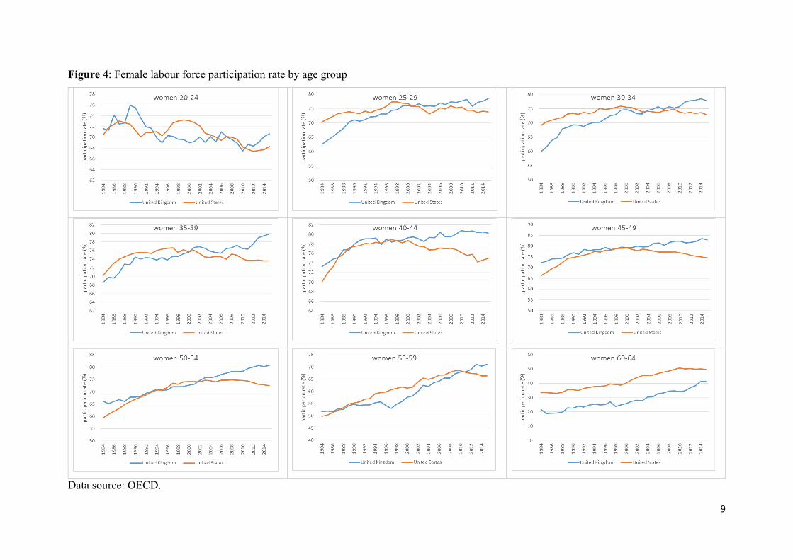
The falling participation rate in the US is often discussed as mainly relating to men (e.g.

Eberstadt, 2017), or even as concentrated among middle-aged men. However, the

comparative patterns for the participation rate since 1984 disaggregated by gender and age

group, shown in Figure 3 for men and Figure 4 for women, tell a different story. They show

participation rates in the US from 2000 falling substantially for men in each age group up to

54, with those over 60 being the only ones to see an increase. For women up to age 50 there

is also some decline over that period, though much less pronounced than for men and varying

across age groups. What is striking, though, is that for men the decline since 2000 represents

a continuation of a longer-term trend (albeit accelerated during the crisis), whereas for

women it is a reversal of the upward trajectory seen up to that point. In the UK, by contrast,

the male participation rate also declined up to 2000 for most age groups, but by 2017 it was

generally as high as in 2000 or higher (except for youngest age group), and the rate for

women aged 25 or over has continued to rise. As a result, participation rates are now higher

in the UK than the US for both men and women in each age group up to the age of 60.

8

Figure 3: Male labour force participation rate by age group

Data source: OECD.

9

Figure 4: Female labour force participation rate by age group

Data source: OECD.

10

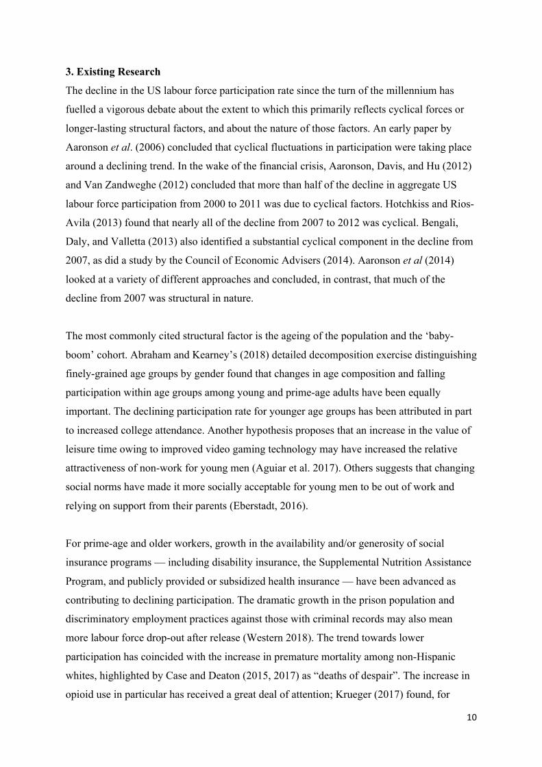
3. Existing Research

The decline in the US labour force participation rate since the turn of the millennium has

fuelled a vigorous debate about the extent to which this primarily reflects cyclical forces or

longer-lasting structural factors, and about the nature of those factors. An early paper by

Aaronson et al. (2006) concluded that cyclical fluctuations in participation were taking place

around a declining trend. In the wake of the financial crisis, Aaronson, Davis, and Hu (2012)

and Van Zandweghe (2012) concluded that more than half of the decline in aggregate US

labour force participation from 2000 to 2011 was due to cyclical factors. Hotchkiss and Rios-

Avila (2013) found that nearly all of the decline from 2007 to 2012 was cyclical. Bengali,

Daly, and Valletta (2013) also identified a substantial cyclical component in the decline from

2007, as did a study by the Council of Economic Advisers (2014). Aaronson et al (2014)

looked at a variety of different approaches and concluded, in contrast, that much of the

decline from 2007 was structural in nature.

The most commonly cited structural factor is the ageing of the population and the ‘baby-

boom’ cohort. Abraham and Kearney’s (2018) detailed decomposition exercise distinguishing

finely-grained age groups by gender found that changes in age composition and falling

participation within age groups among young and prime-age adults have been equally

important. The declining participation rate for younger age groups has been attributed in part

to increased college attendance. Another hypothesis proposes that an increase in the value of

leisure time owing to improved video gaming technology may have increased the relative

attractiveness of non-work for young men (Aguiar et al. 2017). Others suggests that changing

social norms have made it more socially acceptable for young men to be out of work and

relying on support from their parents (Eberstadt, 2016).

For prime-age and older workers, growth in the availability and/or generosity of social

insurance programs — including disability insurance, the Supplemental Nutrition Assistance

Program, and publicly provided or subsidized health insurance — have been advanced as

contributing to declining participation. The dramatic growth in the prison population and

discriminatory employment practices against those with criminal records may also mean

more labour force drop-out after release (Western 2018). The trend towards lower

participation has coincided with the increase in premature mortality among non-Hispanic

whites, highlighted by Case and Deaton (2015, 2017) as “deaths of despair”. The increase in

opioid use in particular has received a great deal of attention; Krueger (2017) found, for

11

example, that labour force participation fell more in areas where relatively more opioid pain

medication has been prescribed, though causality likely runs in both directions.1

While much of the attention has focused on men, some of these drivers also apply to women,

and other factors that may have contributed to the levelling-off in female labour force

participation have also received attention. Blau and Kahn (2013) is among the studies

highlighting the absence in the US of family-friendly policies such as paid parental leave.

Caring for elderly parents may also be a factor, with the share of prime-age workers who

have eldercare responsibilities increasing as the baby boom cohort ages. The importance of

gender role attitudes has also been debated, with respect for example to the hypothesis that

highly educated women have been increasingly ‘opting out’ (Goldin and Katz, 2008; Herr

and Wolfram, 2012) or that there has been a ‘rebound in traditional gender role attitudes’

(Fortin, 2015).

With a great deal of attention paid in recent US research to the displacement of workers by a

combination of globalization and technological change, including robotisation, some have

argued that disappointing levels of participation reflect a growing mismatch between

available workers and vacant jobs. The extent to which this is seen in the data, and if so

whether it represents a short-term feature of the recession rather than a longer-term and more

structural phenomenon, is contested. A related debate is about the extent to which declining

rates of geographic mobility have led to lower rates of employment. Molloy, Smith, and

Wozniak (2011), for example, document that internal migration rates have trended steadily

downward over the past 25 years and are now lower than at any previous time in the post-war

period.

For the UK, research has focused on the relatively limited job loss and unemployment

increase during the Great Recession compared with previous downturns, and on the sharp

recovery in the employment rate since 2012. This is generally linked to what happened to

pay, with the UK seeing the biggest fall in real wages of any G7 country (Taylor, Jowett and

Hardie, 2014), fairly uniform across sectors, so the focus of research has been as much on

why wages have performed so poorly. The UK’s high degree of labour market ‘flexibility’ is

1 Among the few such results available in the research literature, quasi-experimental evidence for Denmark shows that a 10 percentage point higher opioid prescription rate leads to a 1.5 percentage point decrease in labour force participation for an average individual (Laird and Nielsen, 2016).

12

often advanced as a key factor, but as Coulter (2016) points out, this does not help to explain

why the Great Recession was so different from previous recessions since many of the key

reforms aimed at increasing flexibility were enacted in the late 1980s, and during the 1990s

recession employment, rather than wages, bore the brunt of the shock. Research suggests that

more people are willing to work at a given real wage and/or are less responsive to falls in the

real wage (Disney, Jin and Miller 2013), but it is not clear why this would be the case. An

aspect that has received attention is capital ‘shallowing’ as opposed to deepening: the fall in

the price of labour relative to the cost of capital may have encouraged firms to substitute

labour for equipment. Pessoa and Van Reenen (2014) argue that this accounts for up to half

of the fall in labour productivity since the start of the Great Recession, with a

correspondingly large impact on employment.

A sharp increase in labour market polarisation was also seen in the UK during the recession,

with low-skilled jobs expanding their share and medium-skilled jobs continuing to decline

(Plunkett and Pessoa 2013), and sectoral shifts may also have been important in the evolution

of average real wages with some higher paying sectors experiencing falls in employment and

a marked shift from public to private sector employment. Inward migration may have been

associated with greater willingness to work in insecure sectors and for lower pay, though

empirical studies have not found a statistically significant impact from EU migration on

native employment outcomes (Devlin et al., 2014). Changes in social transfers from 2010,

reducing their generosity and increasing conditionality in terms of job search, might have

reduced the reservation wage for some. Enhanced family policy may also have played a role

in boosting female participation.

4. Method and Data

We now set out our approach to understanding the evolution of labour force participation

over time in the US and the UK, and how this relates to previous US studies. A useful point

of departure is the Aaronson et al (2006) study employing a cohort-based model.2 In this

modelling strategy, participation rates are analysed separately by age group and gender.

Controls include only aggregate variables, where aggregation is specific to the different

gender and age groups. The controls include the share of individuals with high/low education,

2 The same methodology is used, among others, by the European Commission in its 2015 Ageing Report – see EC (2014, 2015).

13

the share of individuals living in different types of households (e.g. with/without a partner,

with/without children), the share of individuals with disabilities, measures of earning

potentials such as the (age-specific) gender wage gap, measures of (average) household

wealth, measures for business cycle effects, and proxies for the relevant social programs,

such as the availability of childcare for women in childbearing years, and the fraction of

individuals eligible for early retirement in older cohorts. Because each gender-age subgroup

provides one unit of observation, the identification of the effects of each determinant can be

obtained only by exploiting its variation over time. Time invariant cohort effects are also

included. Aggregation over the different gender-age categories is obtained by weighting the

participation rates in each subgroup by the population size of that subgroup.

However, the group-level analysis suffers from what is known as the “ecological fallacy” (see

Appendix A). Using micro-data helps to avoid this problem, and it also allows to control for

more characteristics.3 This is the strategy used, for instance, by Aaronson et al. (2012), who

estimate the probability of being in the labour force at the individual level, separately by

gender and age groups, in order to allow the cohort effects and other controls to flexibly vary

across age, gender, and education. They control for age, year of birth, race, education, the

business cycle, plus include additional conditioning variables for specific demographic

groups, like the real state minimum wage and the ratio of the average youth hourly wage to

average adult hourly wage for the younger age groups, indicators for being married with

children and married with a young child for the middle age groups, and gender-specific life

expectancies for the older age groups.

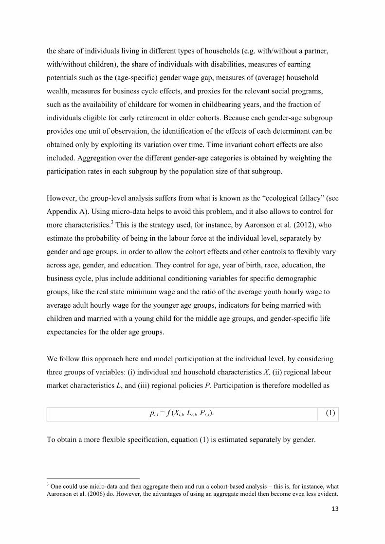
We follow this approach here and model participation at the individual level, by considering

three groups of variables: (i) individual and household characteristics X, (ii) regional labour

market characteristics L, and (iii) regional policies P. Participation is therefore modelled as

pi,t = f (Xi,t, Lr,t, Pr,t). (1)

To obtain a more flexible specification, equation (1) is estimated separately by gender.

3 One could use micro-data and then aggregate them and run a cohort-based analysis – this is, for instance, what Aaronson et al. (2006) do. However, the advantages of using an aggregate model then become even less evident.

14

One major challenge for this comparative exercise is obtaining consistent and homogeneous

data, meaning that variables have the same meaning irrespective of time and space.4 We use

the Labour Force Survey (LFS) for the UK and the Current Population Survey (CPS) for the

US. For each year, we select the second quarter LFS for the UK and the March CPS for the

US, because these particular surveys contain additional information. Our data are repeated

cross-sections.

Most of the data constraints are in the UK data, as the Office for National Statistics does not

attempt to homogenize variables in the face of significant changes in the questionnaire over

the years. We select only variables that can be traced back with a sufficient level of reliability

(allowing minor changes in the filtering conditions or categorical values). There is a tradeoff

between the number of variables that can be included and the length of the time series. We

focus on the period between 1996 and 2017, as information on educational levels, health

status, home ownership, and household composition prior to 1996 becomes difficult to

compare with more recent waves. As conservative as this choice can appear, it still precludes

the use of retrospective information, in particular the labour market status of individuals in

previous periods, which is only available from 2011 onwards. However, while participation

in the past is possibly the single most important predictor of current participation, its

inclusion would in any case have been problematic. This is because, without controlling for

individual effects (which is possible only using panel data), the lagged endogenous variable

will soak up the effects of unobserved heterogeneity, hence introducing an upward bias in

true state persistence. Finally, in the LFS it is not possible to reconstruct the labour market

status of partners.

While these data limitations with respect to the UK constrain our choices of covariates for the

US, we end up with datasets for the two countries that are highly comparable. The differences

are:

• Health: We define “bad health” in the UK data as having a health problem that limits

the kind of paid work that the respondent can do, while in the US data we define it as

being in the lower two categories of five-category self-reported health status. The

4 This does not prevent us from including country-specific covariates in some of the models, when appropriate.

15

resulting fraction of individuals with “bad” health is larger in the UK than in the US,

as shown in the descriptive statistics (see Table 1).

• Race: A dummy for Hispanic is added for the US.

• Household type: The US data allow distinguishing married couples living together

from married individuals living with a partner outside marriage. We follow the UK

definition and distinguish only between married individuals living alone and married

individuals living with their partner, irrespective of whether the partner is their spouse

or not.

• Children: The UK data provide dummies for the presence of children of different ages

(under 2, 2-4, 5-9, 10-15) in the household. They do not provide information on the

number of children in each age group. The US data records the overall number of

children and the age of the youngest and the oldest child. From this we reconstructed

dummies for the youngest children being in each relevant age group (under 2, 2-4, 5-

9, 10-15). Consequently, it is possible that all flags related to children are switched on

in the UK data while in the US data they are mutually exclusive.

• Home ownership: In the UK data it is possible to distinguish between whether the

house is owned outright or with an ongoing mortgage. Information on mortgages is

available only from 2010 onwards in the US data and is therefore not included.

Data for social policies come from the OECD Social Policy database. They include the

amount of social expenditures for family policies and the amount of total social expenditures,

both as a percentage of GDP.

Data for family policies are taken from the OECD Family database. The variables selected

are Maternity total protected weeks, defined as the maximum weeks of job-protected

maternity, parental and home care leave available to mothers, regardless of income support,

maternity total paid weeks, the total weeks of paid maternity, parental and home care

payments available to mothers, paternity total specific weeks, the total weeks of leave

reserved for exclusive use by the father, and paternity specific paid weeks,the total weeks of

paid leave reserved for exclusive use by the father. Data are restricted to 2016 for the US.

16

In the analysis of the US, we use additional state-level policy information provided by the

University of Kentucky Center for Poverty Research (UKCPR).5 In particular, we consider

the following variables: AFCD/TANF/SNAP, the combined monthly maximum AFDC/TANF

and Food Stamps benefits for a 4-person family; EITC2max, the EITC maximum credit for 2

dependents; EITC state, the state EITC credit as percentage of the federal credit; and SSI

federal, the monthly maximum federal SSI benefits for individuals living independently.6

The minimum wage is at the national level for the UK. For the US, we use the state minimum

wage, as provided by the UKCPR.

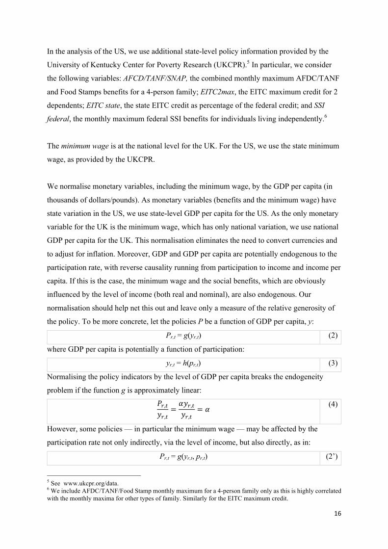
We normalise monetary variables, including the minimum wage, by the GDP per capita (in

thousands of dollars/pounds). As monetary variables (benefits and the minimum wage) have

state variation in the US, we use state-level GDP per capita for the US. As the only monetary

variable for the UK is the minimum wage, which has only national variation, we use national

GDP per capita for the UK. This normalisation eliminates the need to convert currencies and

to adjust for inflation. Moreover, GDP and GDP per capita are potentially endogenous to the

participation rate, with reverse causality running from participation to income and income per

capita. If this is the case, the minimum wage and the social benefits, which are obviously

influenced by the level of income (both real and nominal), are also endogenous. Our

normalisation should help net this out and leave only a measure of the relative generosity of

the policy. To be more concrete, let the policies P be a function of GDP per capita, y:

Pr,t = g(yr,t) (2)

where GDP per capita is potentially a function of participation:

yr,t = h(pr,t) (3)

Normalising the policy indicators by the level of GDP per capita breaks the endogeneity

problem if the function g is approximately linear:

!",$%",$

= '%",$%",$

= ' (4)

However, some policies — in particular the minimum wage — may be affected by the

participation rate not only indirectly, via the level of income, but also directly, as in:

Pr,t = g(yr,t, pr,t) (2’)

5 See www.ukcpr.org/data. 6 We include AFDC/TANF/Food Stamp monthly maximum for a 4-person family only as this is highly correlated with the monthly maxima for other types of family. Similarly for the EITC maximum credit.

17

This could happen if politicians see the minimum wage as a way to influence participation.

Our normalisation is not safe against this possibility. This suggests caution is needed in

interpreting the coefficient for the (normalised) minimum wage.

We end up with 1,550,258 observations for the UK and 2,528,122 observations for the US.

Minimum legal working age is 16 in the UK and 14 in the US, with limits on the number of

hours worked by minors under the age of 16. Hence, we focus on the 16-and-over population.

As labour market status is not recorded in the UK data for individuals above state pension age

unless they are working, and state pension age has changed over the years, we restrict our

analysis to females under 60 and males under 65.

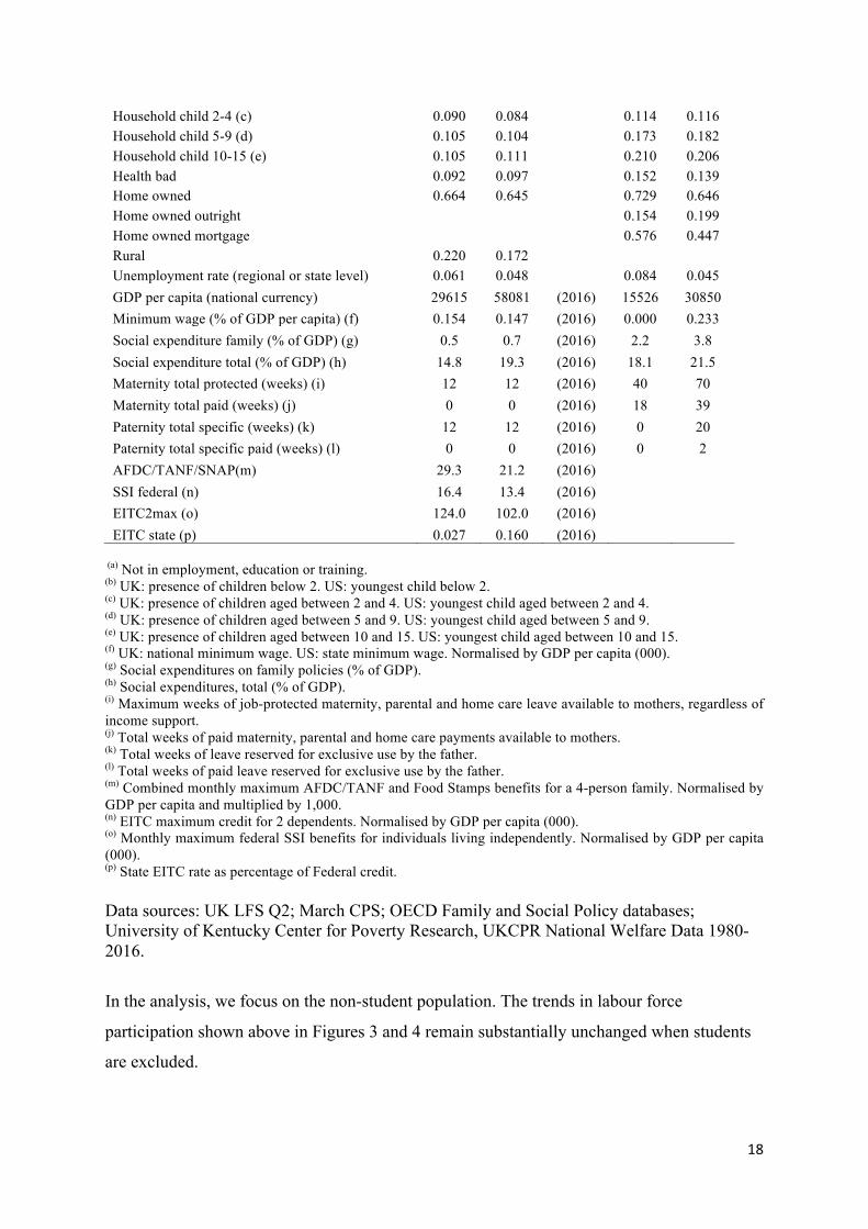
Average values for the variables we include in the analysis, in the initial and final year, are

reported in Table 1.

Table 1: Average values

US UK 1996 2017 1996 2017 Active 0.775 0.743 0.778 0.798 Student 0.106 0.150 0.070 0.088 NEET (15-24) (a) 0.232 0.220 0.241 0.175 Age 37.0 38.5 38.1 40.1 Year of birth 1959.0 1978.5 1957.9 1976.9 Race black 0.099 0.123 0.015 0.030 Race other 0.049 0.108 0.040 0.103 Hispanic 0.152 0.204 Foreign born 0.150 0.192 0.078 0.177 Foreign national 0.094 0.102 0.047 0.142 Education low 0.202 0.156 0.359 0.164 Education medium 0.581 0.545 0.442 0.447 Education high 0.218 0.299 0.199 0.388 Household single alone 0.272 0.312 0.260 0.283 Household single cohabiting 0.020 0.043 0.054 0.121 Household married alone 0.009 0.013 0.016 0.003 Household married cohabiting 0.565 0.510 0.557 0.487 Household separated alone 0.025 0.019 0.024 0.023 Household separated cohabiting 0.002 0.003 0.004 0.003 Household divorced alone 0.082 0.070 0.052 0.048 Household divorced cohabiting 0.012 0.018 0.019 0.023 Household widowed alone 0.012 0.011 0.013 0.009 Household widowed cohabiting 0.001 0.002 0.001 0.001 Number of children 0.953 0.950 Household child under 2 (b) 0.080 0.065 0.078 0.074

18

Household child 2-4 (c) 0.090 0.084 0.114 0.116 Household child 5-9 (d) 0.105 0.104 0.173 0.182 Household child 10-15 (e) 0.105 0.111 0.210 0.206 Health bad 0.092 0.097 0.152 0.139 Home owned 0.664 0.645 0.729 0.646 Home owned outright 0.154 0.199 Home owned mortgage 0.576 0.447 Rural 0.220 0.172 Unemployment rate (regional or state level) 0.061 0.048 0.084 0.045 GDP per capita (national currency) 29615 58081 (2016) 15526 30850 Minimum wage (% of GDP per capita) (f) 0.154 0.147 (2016) 0.000 0.233 Social expenditure family (% of GDP) (g) 0.5 0.7 (2016) 2.2 3.8 Social expenditure total (% of GDP) (h) 14.8 19.3 (2016) 18.1 21.5 Maternity total protected (weeks) (i) 12 12 (2016) 40 70 Maternity total paid (weeks) (j) 0 0 (2016) 18 39 Paternity total specific (weeks) (k) 12 12 (2016) 0 20 Paternity total specific paid (weeks) (l) 0 0 (2016) 0 2 AFDC/TANF/SNAP(m) 29.3 21.2 (2016) SSI federal (n) 16.4 13.4 (2016) EITC2max (o) 124.0 102.0 (2016) EITC state (p) 0.027 0.160 (2016)

(a) Not in employment, education or training. (b) UK: presence of children below 2. US: youngest child below 2. (c) UK: presence of children aged between 2 and 4. US: youngest child aged between 2 and 4. (d) UK: presence of children aged between 5 and 9. US: youngest child aged between 5 and 9. (e) UK: presence of children aged between 10 and 15. US: youngest child aged between 10 and 15. (f) UK: national minimum wage. US: state minimum wage. Normalised by GDP per capita (000). (g) Social expenditures on family policies (% of GDP). (h) Social expenditures, total (% of GDP). (i) Maximum weeks of job-protected maternity, parental and home care leave available to mothers, regardless of income support. (j) Total weeks of paid maternity, parental and home care payments available to mothers. (k) Total weeks of leave reserved for exclusive use by the father. (l) Total weeks of paid leave reserved for exclusive use by the father. (m) Combined monthly maximum AFDC/TANF and Food Stamps benefits for a 4-person family. Normalised by GDP per capita and multiplied by 1,000. (n) EITC maximum credit for 2 dependents. Normalised by GDP per capita (000). (o) Monthly maximum federal SSI benefits for individuals living independently. Normalised by GDP per capita (000). (p) State EITC rate as percentage of Federal credit. Data sources: UK LFS Q2; March CPS; OECD Family and Social Policy databases; University of Kentucky Center for Poverty Research, UKCPR National Welfare Data 1980-2016.

In the analysis, we focus on the non-student population. The trends in labour force

participation shown above in Figures 3 and 4 remain substantially unchanged when students

are excluded.

19

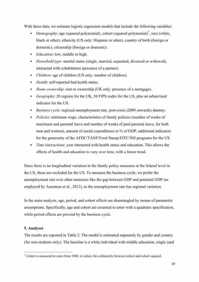
With these data, we estimate logistic regression models that include the following variables:

• Demography: age (squared polynomial), cohort (squared polynomial)7, race (white,

black or other), ethnicity (US only: Hispanic or other), country of birth (foreign or

domestic), citizenship (foreign or domestic).

• Education: low, middle or high.

• Household type: marital status (single, married, separated, divorced or widowed),

interacted with cohabitation (presence of a partner).

• Children: age of children (US only: number of children).

• Health: self-reported bad health status.

• Home ownership: rent or ownership (UK only: presence of a mortgage).

• Geography: 20 regions for the UK, 56 FIPS codes for the US, plus an urban/rural

indicator for the US.

• Business cycle: regional unemployment rate, post-crisis (2009 onwards) dummy.

• Policies: minimum wage, characteristics of family policies (number of weeks of

maximum and parental leave and number of weeks of paid parental leave, for both

men and women), amount of social expenditures in % of GDP, additional indicators

for the generosity of the AFDC/TANF/Food Stamp/EITC/SSI programs for the US.

• Time interactions: year interacted with health status and education. This allows the

effects of health and education to vary over time, with a linear trend.

Since there is no longitudinal variation in the family policy measures at the federal level in

the US, these are excluded for the US. To measure the business cycle, we prefer the

unemployment rate over other measures like the gap between GDP and potential GDP (as

employed by Aaronson et al., 2012), as the unemployment rate has regional variation.

In the main analysis, age, period, and cohort effects are disentangled by means of parametric

assumptions. Specifically, age and cohort are assumed to enter with a quadratic specification,

while period effects are proxied by the business cycle.

5. Analyses

The results are reported in Table 2. The model is estimated separately by gender and country

(for non-students only). The baseline is a white individual with middle education, single (and

7 Cohort is measured in years from 1900, to reduce the collinearity between cohort and cohort squared.

20

not cohabiting), renting (rather than owning), who lives in London (UK) or urban California

(US).

Table 2: Logit estimates of the probability of being in the labour force

(1) (2) (3) (4) US UK US UK

Male Male Female Female Variables 16-64 16-64 16-59 16-59 Age 0.123 *** 0.178 *** 0.076 *** 0.156 *** Age squared -0.002 *** -0.003 *** -0.001 *** -0.002 *** Year of birth 0.029 *** 0.047 *** 0.034 *** 0.056 *** Year of birth squared 0.000 *** 0.000 *** 0.000 *** 0.000 *** Race black -0.479 *** -0.315 *** 0.174 *** 0.231 *** Race other -0.367 *** -0.447 *** -0.109 *** -0.712 *** Foreign born 0.311 *** 0.222 *** 0.003 -0.063 *** Foreign national 0.112 *** -0.082 *** -0.519 *** -0.043 *** Hispanic 0.111 *** 0.105 *** Education high -31.25 *** -4.44 -24.42 *** 10.35 *** Education low 3.050 5.772 * -13.140 *** 25.070 *** Health bad -8.532 ** -47.640 *** 29.210 *** 0.993 Year x health 0.003 * 0.023 *** -0.015 *** -0.001 Year x education high 0.016 *** 0.002 0.012 *** -0.005 *** Year x education low -0.002 -0.003 * 0.006 *** -0.013 *** Household single cohab 0.735 *** 0.617 *** 0.191 *** 0.212 *** Household married alone 0.639 *** 0.804 *** -0.050 * -0.167 *** Household married cohab 0.899 *** 0.730 *** -0.384 *** -0.141 *** Household separated alone 0.443 *** 0.361 *** 0.200 *** 0.037 * Household separated cohab 0.548 *** 1.030 *** 0.063 0.399 *** Household divorced alone 0.486 *** 0.307 *** 0.315 *** 0.206 *** Household divorced cohab 0.793 *** 0.689 *** 0.197 *** 0.300 *** Household widowed alone 0.133 *** 0.238 *** -0.431 *** -0.084 *** Household widowed cohab 0.351 *** 0.544 *** -0.248 *** 0.059 Household child under 2 0.041 -0.114 *** -0.967 *** -1.479 *** Household child 2-4 0.013 -0.205 *** -0.645 *** -1.283 *** Household child 5-9 0.067 *** -0.225 *** -0.285 *** -0.759 *** Household child 10-15 0.169 *** -0.145 *** 0.071 *** -0.429 *** Number of children 0.139 *** -0.094 *** Home owned 0.068 *** 0.182 *** Unemployment rate -1.215 *** -0.023 0.615 ** -0.038 Post-crisis 0.116 *** 0.089 ** 0.083 *** 0.043 Minimum wage -0.546 -0.243 * 0.910 *** -0.010 Social expenditure family -0.104 ** -0.031 0.091 ** 0.005 Social expenditure total -0.008 -0.010 -0.021 ** -0.008 AFDC/TANF/SNAP -0.014 *** -0.018 *** SSI federal 0.003 0.022 EITC2max 0.000 0.000 EITC state -0.022 0.019 Rural -0.137 *** 0.007 Home owned outright 0.240 *** 0.320 ***

21

Home owned mortgage 1.232 *** 1.056 *** Maternity total protected -0.007 *** -0.008 *** Maternity total paid 0.006 *** 0.000 Paternity total specific 0.007 * 0.007 *** Constant 1.127 *** -0.792 0.461 ** -3.431 ***

Observations 1063351 718417 1053301 704235 chi2 97216 120525 79867 120176 P 0.000 0.000 0.000 0.000 r2_p 0.239 0.364 0.118 0.246 Robust standard errors in parentheses *** p<0.01, ** p<0.05, * p<0.1

Note: Students excluded. The baseline is a medium education white individual, single and not cohabiting, living in urban California (US) or central London (UK), and renting. Cohort is measured subtracting 1,900 from year of birth. State (US) and NUTS1 (UK) regional dummies included.

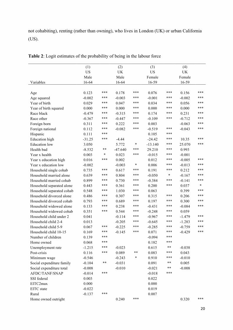
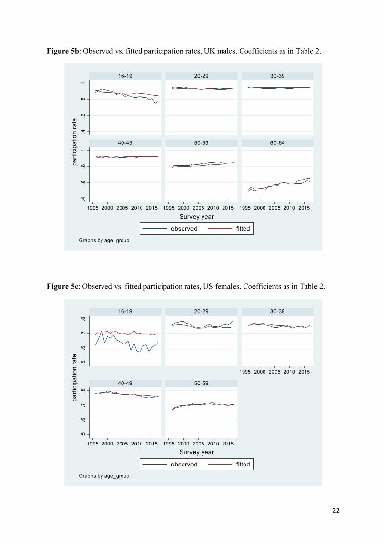
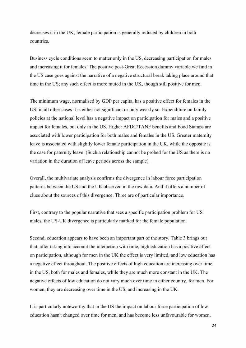
Figures 5a-d show the actual versus estimated participation rates. Apart from the age group

16-19, where the population of non-students is very small, the goodness of fit is high.

Figure 5a: Observed vs. fitted participation rates, US males. Coefficients as in Table 2.

22

Figure 5b: Observed vs. fitted participation rates, UK males. Coefficients as in Table 2.

Figure 5c: Observed vs. fitted participation rates, US females. Coefficients as in Table 2.

23

Figure 5d: Observed vs. fitted participation rates, UK females. Coefficients as in Table 2.

Most of the estimated effects in Table 2 go in the expected direction. In both countries, being

black reduces ceteris paribus participation for males and increases it for females. Male

immigrants (born outside the country) are more likely to be in the labour force in both

countries, all else equal, whereas for women that effect is insignificant in the US and negative

in the UK. Hispanics participate more in the US, whether male or female. Living with a

partner outside marriage increases participation for both genders, compared to living alone,

while marriage increases participation for males and decreases it for females. Being separated

or divorced increases participation for both genders. Widowhood increases participation for

males and decreases it for females. Home ownership is associated with increased

participation, and in the UK (whether outright owners versus those with mortgages can be

distinguished) this is most pronounced in presence of a mortgage; it should be noted, though,

that causality could well go in the other direction, from participation to home ownership.8

Having older children in the household increases participation for males in the US but

8 This could also be a concern for other variables, if less clear-cut. For instance, not participating in the labour market could affect self-perceived health status, while participation could sometimes be a positive for the likelihood of marriage.

24

decreases it in the UK; female participation is generally reduced by children in both

countries.

Business cycle conditions seem to matter only in the US, decreasing participation for males

and increasing it for females. The positive post-Great Recession dummy variable we find in

the US case goes against the narrative of a negative structural break taking place around that

time in the US; any such effect is more muted in the UK, though still positive for men.

The minimum wage, normalised by GDP per capita, has a positive effect for females in the

US; in all other cases it is either not significant or only weakly so. Expenditure on family

policies at the national level has a negative impact on participation for males and a positive

impact for females, but only in the US. Higher AFDC/TANF benefits and Food Stamps are

associated with lower participation for both males and females in the US. Greater maternity

leave is associated with slightly lower female participation in the UK, while the opposite is

the case for paternity leave. (Such a relationship cannot be probed for the US as there is no

variation in the duration of leave periods across the sample).

Overall, the multivariate analysis confirms the divergence in labour force participation

patterns between the US and the UK observed in the raw data. And it offers a number of

clues about the sources of this divergence. Three are of particular importance.

First, contrary to the popular narrative that sees a specific participation problem for US

males, the US-UK divergence is particularly marked for the female population.

Second, education appears to have been an important part of the story. Table 3 brings out

that, after taking into account the interaction with time, high education has a positive effect

on participation, although for men in the UK the effect is very limited, and low education has

a negative effect throughout. The positive effects of high education are increasing over time

in the US, both for males and females, while they are much more constant in the UK. The

negative effects of low education do not vary much over time in either country, for men. For

women, they are decreasing over time in the US, and increasing in the UK.

It is particularly noteworthy that in the US the impact on labour force participation of low

education hasn't changed over time for men, and has become less unfavourable for women.

25

This is contrary to the popular story that changes in the labour market have made it much

more difficult or less attractive for Americans with limited education to participate.

Over the period covered by our analysis, 1996 to 2017, the proportion of the working-aged

population with low education fell much more rapidly in the UK than in the US. The decline

in the UK was 20 percentage points, versus just 4 percentage points in the US (Table 1). This

difference in compositional shift is likely to have had a large effect on the differing labour

force participation trends in the two countries. Similarly, the share with high education

increased by 18 percentage points in the UK, compared to 8 percentage points in the US

(Table 1). Although the effects of high education increased over time in the US but not in the

UK, the compositional shift is likely to have overwhelmed this and thus contributed to the

better labour force participation trend in the UK.

Table 3: Effects of education and health over time.

Males Females US UK US UK

Case Reference category 1996 2017 1996 2017 1996 2017 1996 2017

Education High Education Medium 0.29 0.62 0.04 0.08 0.33 0.59 0.57 0.47

Education Low Education Medium -0.58 -0.62 -0.40 -0.46 -0.80 -0.67 -0.48 -0.75

Health Bad Health Good -2.16 -2.10 -2.73 -2.26 -1.33 -1.65 -1.90 -1.93

Note: the table reports the contribution to the logit score from Table 2. The non-linearity of the logit

function means that the same increase in the logit score has a different impact on the estimated

probability depending on the starting value of the score.

A third key finding is that health appears to have mattered less than some have hypothesized.

In Table 3 we see that bad (self-reported) health has a negative effect on participation. The

negative effects of bad health remain more or less constant over time for US males and UK

females, whereas they get smaller (less negative) for UK males and larger (more negative) for

US females. So in the US case, where the relationship between health and participation for

men has been such a focus in recent debate, there is no evidence that those in bad health have

become less likely to participate over time; it is only for women that any such pattern is seen.

The proportion reporting their health to be 'bad' rose only marginally in the US (Table 1).

This lack of a significant rise, coupled with the fact that the impact of health didn't change for

26

individuals, casts doubt on the much-discussed role of increasing levels of ill-health and the

opioid crisis in reducing labour force participation in the United States.

How much have cyclical forces mattered? Our strategy for distinguishing the role of cyclical

factors relative to structural factors in accounting for the differing over-time patterns in the

US and the UK is to examine age, period, and cohort effects. Age and cohort effects, as well

as the effects of the other characteristics analysed above, are considered ‘structural’. The so-

called 'period' effect, which we measure through macroeconomic variables, captures the

cyclical component.

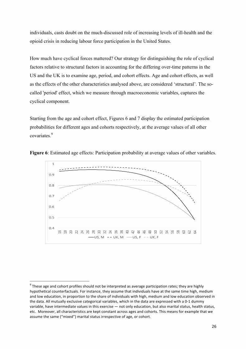
Starting from the age and cohort effect, Figures 6 and 7 display the estimated participation

probabilities for different ages and cohorts respectively, at the average values of all other

covariates.9

Figure 6: Estimated age effects: Participation probability at average values of other variables.

9Theseageandcohortprofilesshouldnotbeinterpretedasaverageparticipationrates;theyarehighly

hypotheticalcounterfactuals.Forinstance,theyassumethatindividualshaveatthesametimehigh,medium

andloweducation,inproportiontotheshareofindividualswithhigh,mediumandloweducationobservedin

thedata.Allmutuallyexclusivecategoricalvariables,whichinthedataareexpressedwitha0-1dummy

variable,haveintermediatevaluesinthisexercise—notonlyeducation,butalsomaritalstatus,healthstatus,

etc.Moreover,allcharacteristicsarekeptconstantacrossagesandcohorts.Thismeansforexamplethatwe

assumethesame(“mixed”)maritalstatusirrespectiveofage,orcohort.

27

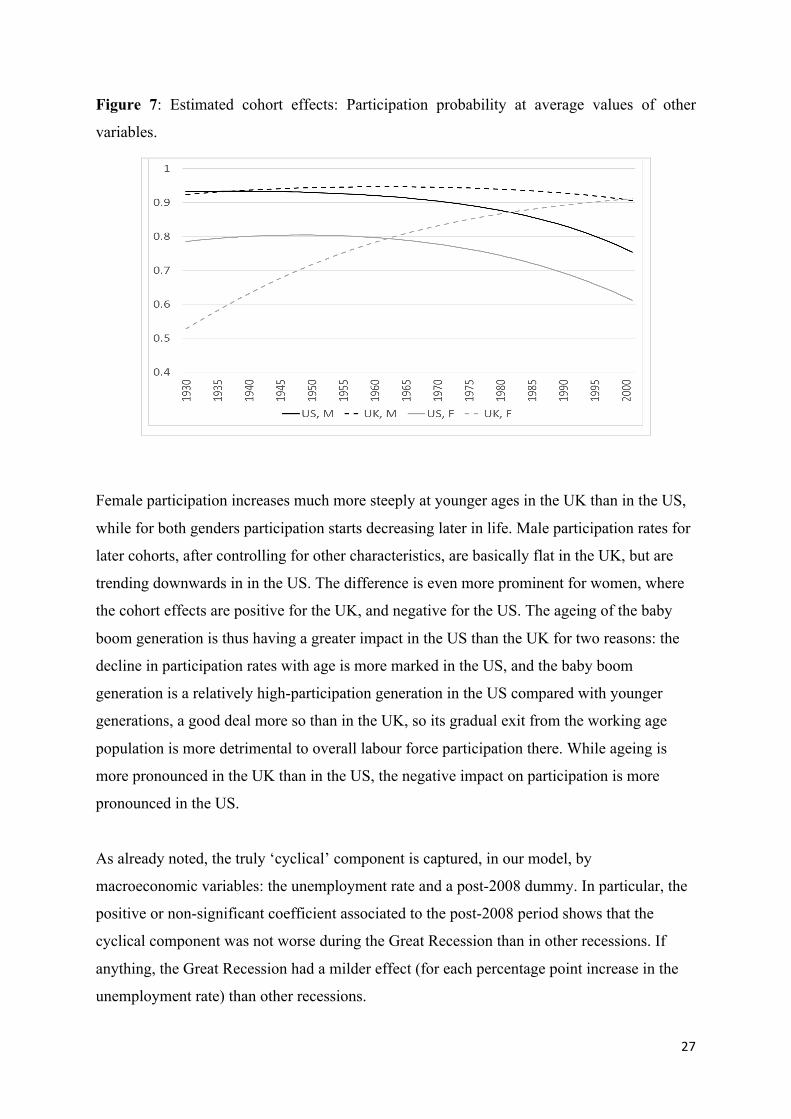
Figure 7: Estimated cohort effects: Participation probability at average values of other

variables.

Female participation increases much more steeply at younger ages in the UK than in the US,

while for both genders participation starts decreasing later in life. Male participation rates for

later cohorts, after controlling for other characteristics, are basically flat in the UK, but are

trending downwards in in the US. The difference is even more prominent for women, where

the cohort effects are positive for the UK, and negative for the US. The ageing of the baby

boom generation is thus having a greater impact in the US than the UK for two reasons: the

decline in participation rates with age is more marked in the US, and the baby boom

generation is a relatively high-participation generation in the US compared with younger

generations, a good deal more so than in the UK, so its gradual exit from the working age

population is more detrimental to overall labour force participation there. While ageing is

more pronounced in the UK than in the US, the negative impact on participation is more

pronounced in the US.

As already noted, the truly ‘cyclical’ component is captured, in our model, by

macroeconomic variables: the unemployment rate and a post-2008 dummy. In particular, the

positive or non-significant coefficient associated to the post-2008 period shows that the

cyclical component was not worse during the Great Recession than in other recessions. If

anything, the Great Recession had a milder effect (for each percentage point increase in the

unemployment rate) than other recessions.

28

Robustness checks on our specification for the APC analysis are performed in Appendix B.

Given the centrality of structural factors, we are particularly interested in understanding the

relative importance of differences in the composition of the population (endowments) versus

differences in behaviour (as reflected in the estimated coefficients in our models) in

explaining the different trajectories of participation in the US and the UK. For example, are

these driven by changes in the age or education profile of the working-age population, or by

changes in the likelihood that someone of a given age and education will be participating?

We explore this by means of an Oaxaca-Blinder decomposition exercise for logit models, the

standard approach employed in such contexts. The details of this analysis are in Appendix C.

The Oaxaca-Blinder decomposition focuses on whether that part of the structural component

attributable to specific covariates reflects composition effects or behavioural effects.

The answer is both, with approximately equal impact. Dividing our sample into two sub-

periods, 1996-2007 and 2008-2017, we decomposed the average difference in participation

between the two countries into the difference attributable to ‘endowments/characteristics’ of

the working-age population versus ‘behaviour’ as reflected in the estimated coefficients on

these characteristics in our econometric models. For men, there was a negligible average

participation gap between the two countries in the first period, whereas by the second period

a substantial gap had emerged. In the first period, the “endowments” of the working-age

population were more positive for participation in the US, but this was almost exactly offset

by negative behavioural effects. By 2008-2017, the positive effect of endowments for the US

in reducing the participation gap had effectively disappeared, while the negative effect of

coefficients had also increased substantially. In the earlier period US women had an even

greater advantage over their UK counterparts than men in terms of employment-related

characteristics; by the latter period this had fallen by three-quarters, and the effect of

coefficients/behaviours in widening the participation gap were also greater. For both men and

women, the overall deterioration in US participation rates vis-à-vis the UK is quite evenly

split between changes in endowments and in coefficients.

Behaviour was less favourable to participation in the US in the first period, but this

disadvantage has increased in the second period. For men this is particularly related to the

labour force participation of married men, who had been more likely to participate in the US

than the UK but this is no longer the case. For women the overall behavioural effect reflects

29

relatively small changes for most of the variables, together with an increased effect of general

trends related to age, cohort, and residual effects.

The composition of the population was previously more favourable to participation in the US

than in the UK, but that advantage has been lost, primarily due the rapid increase in

educational attainment in the UK. The share of men with low education in the US went down

only 4 percentage points, from 21% in 1996 to 17%, while in the UK it went down 14

percentage points, from 32% to 18%. The difference is even more striking for women: in the

US, the share of women with low education also went down 4 percentage points, from 19%

in 1996 to 15% in 2017, while in the UK it went down a spectacular 25 percentage points,

from 40% to 15%. High education also plays a role. The share of men with high education

went up only 5 percentage points in the US, from 23% in 1996 to 28% in 2017, while in the

UK it went up 16 percentage points, from 21% to 37%. For women, the difference is again

more pronounced. The share of women with high education in the US went up 11 percentage

points, from 21% in 1996 to 32% in 2017, while in the UK it went up 22 percentage points,

from 19% to 41%.

6. The US-UK Contrast in Broader Comparative Context

The turnaround in US labour force participation, from rapid increase in the 1980s and 1990s

to decline in both absolute and relative (to other nations) terms since 2000, is a puzzling

development. We have attempted to understand the American experience via an in-depth

comparison with the United Kingdom, a country that is similar in labour market regulation

and monetary governance and that experienced comparable employment performance up to

2000.

Our analysis suggests three core conclusions. First, the weakening of US labour force

participation is not mainly a story of (white) males. The decline in participation has been

even more significant among American women, and for women, unlike for men, this decline

is a change from the pattern that obtained in the 1980s and 1990s. Figures 9a and 9b show

that this conclusion isn't peculiar to our US-UK comparison. We also observe it when we

consider all of the rich longstanding democratic nations. Figure 8a shows labour force

participation rates among prime-working-age (25 to 54) men, and Figure 8b does so for

prime-age women. Among men, the labour force participation rate in the United States has

fallen more rapidly than in most other nations, but the US already had one of the lowest rates

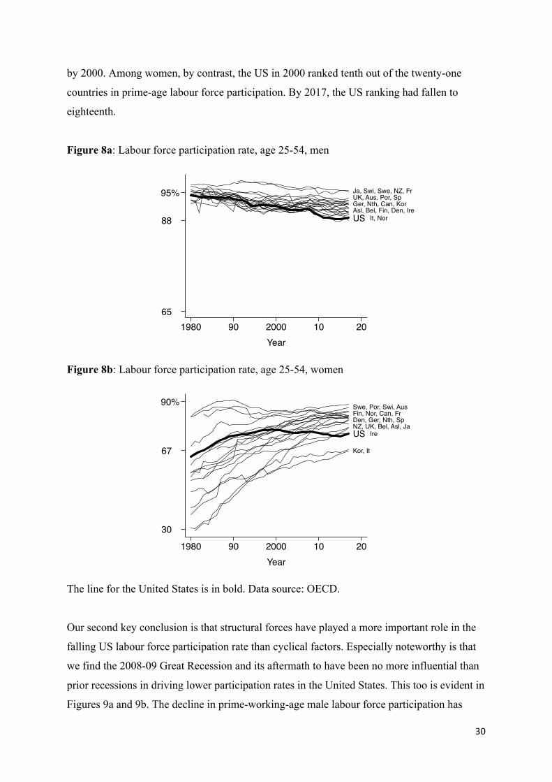
30

by 2000. Among women, by contrast, the US in 2000 ranked tenth out of the twenty-one

countries in prime-age labour force participation. By 2017, the US ranking had fallen to

eighteenth.

Figure 8a: Labour force participation rate, age 25-54, men

Figure 8b: Labour force participation rate, age 25-54, women

The line for the United States is in bold. Data source: OECD.

Our second key conclusion is that structural forces have played a more important role in the

falling US labour force participation rate than cyclical factors. Especially noteworthy is that

we find the 2008-09 Great Recession and its aftermath to have been no more influential than

prior recessions in driving lower participation rates in the United States. This too is evident in

Figures 9a and 9b. The decline in prime-working-age male labour force participation has

US

Ja, Swi, Swe, NZ, FrUK, Aus, Por, SpGer, Nth, Can, KorAsl, Bel, Fin, Den, Ire

It, Nor

65

88

95%

1980 90 2000 10 20Year

US

Swe, Por, Swi, AusFin, Nor, Can, FrDen, Ger, Nth, SpNZ, UK, Bel, Asl, Ja

Ire

Kor, It

30

67

90%

1980 90 2000 10 20Year

31

been a steady pattern over a number of decades, and the decline in female participation has

been a steady pattern since the turn of the century.

Our third conclusion is that the influence of structural forces is a product of both changes in

composition and changes in behaviours. Among these changes, we found a particularly

influential one in the US-UK contrast to be the much slower increase in educational

attainment in the United States.

Here too we can spot this in a broader comparison, as we see in Figures 9a and 9b. Figure 9a

shows the share of 25-to-64-year-olds that have completed less than upper secondary

education. The share of Americans with low education is among the lowest in this group of

nations, but that has been true for decades, and during this period other countries have been

catching up, with their low-educated share falling at a faster rate. In other words, not only the

UK but virtually every other rich democratic nations has been making more rapid progress

than the United States in increasing educational attainment at the low end.

The same is true at the high end, as we see in Figure 9b. This chart shows the share of 25-to-

34-year-olds with a bachelor's degree or more. These data are only available since 2000, but

here too we see the United States starting in a leading position but other nations catching up

quickly, and here even surpassing the US by the 2010s.

Figure 9a: Less than upper secondary education, age 25-64.

US

Por

Sp, It

Bel, Fr, Nth, NZ, AslUK, Den, Nor, Ire, SweAus, Ger, Kor, Swi, Fin

Can

0 9

52%

1980 90 2000 10 20Year

32

Figure 9b: Bachelor's degree or more, age 25-34.

The line for the United States is in bold. Data source: OECD.

In the 1990s and 2000s, the United States was widely viewed as an affluent democratic

country that had comparatively high poverty and inequality but was successful in achieving

high employment (OECD 1994; Scharpf and Schmidt 2000; Kenworthy 2008). This success

was commonly attributed to its comparatively deregulated labour markets, low wages, and

limited taxes and government benefits. America's disappointing employment performance

since the turn of the century suggests this view was either wrong or specific to a particular

historical period.

If an embrace of "low-road capitalism" no longer yields good employment outcomes for the

United States, what will? Our findings suggest that a focus on males or on cyclical patterns is

likely to be of limited help. Longer-term structural developments affecting both men and

even more so women are at the core of the problem. It may well be, as an emerging view

suggests, that an expansion of family-friendly programs such as early education and paid

parental leave would be of considerable help. But our analyses suggest the US might also do

well to turn its attention to educational attainment.

US

NorNth, UKKor, FinDen, Asl

NZ, JaSwe, Can, IreSwi, PorFr, SpBel, ItAusGer

0

20

40%

1980 90 2000 10 20Year

33

References

Aguiar, M., Bils, M., Charles, K. and Hurst, E. (2017). Leisure, Luxuries and the Labor Supply

of Young Men, NBER working paper No. 23552, Cambridge, MA.

Abraham, K. and Kearney, M. (2018). Explaining the Decline in the U.S. Employment-to-

Population Ratio: A Review of the Evidence, NBER Working Paper No. 24333,

Cambridge, MA.

Aronson S, Fallick B, Figura A, Pingle J, Wascher W. (2006). “The Recent Decline in the

Labor Force Participation Rate and Its Implications for Potential Labor Supply.”

Brookings Papers on Economic Activity, 37 (1): 69-154.

Aronson, S., Cajner, T., Fallick, B., Galbis-Reig, F., Smith, C. and Wascher, W. (2014). Labor

Force Participation: Recent Developments and Future Prospects, Finance and Economics

Discussion Series 2014-64, Board of Governors of the Federal Reserve System.

Aronson, D., Davis, J. and Hu, L. (2012). Explaining the decline in the U.S. labor force

participation rate, Chicago Fed Letter issue March, No. 296.

Bengali, L., Daly, M. and Valletta, R. (2013). Will Labor Force Participation Bounce Back?

FRBSF Economic Letter 2013-14, Federal Reserve Board of Sab Francisco.

Blau, F. D. and Kahn, L.M. (2013). “Female Labor Supply: Why Is the US Falling Behind?”

American Economic Review 103: 251-256.

Bullard J (2014). “The Rise and Fall of Labor Force Participation in the United States.” Federal

Reserve Bank of St. Louis Review, First Quarter: 1-12.

Case, A. and Deaton, A.B. (2017). “Mortality and morbidity in the 21st century” Brookings

Papers on Economic Activity conference drafts, March 23-24, 2017.

Chirikos, T.N. (1993). “The relationship between health and labour market status”, Annual

Review of Public Health, 14: 293-312.

Coulter, S. (2016). “The UK Labour Market and the Great Recession”, in M. Myant, S.

Theodoropoulou and A. Piasna, (eds.) Unemployment, Internal Devaluation and Labour

Market Deregulation in Europe. Brussels, European Trade Union Institute, 197-227.

Council of Economic Advisers (2014). The Labor Force Participation Rate Since 2007: Causes

and Policy Implications, Washington, D.C.

Council of Economic Advisers (2014). The Long-Term Decline in the Prime Age Male Labor

Force Participation, Washington, D.C.

Devlin C. et al. (2014) Impact of migration on UK native employment: an analytical review of

the evidence, Occasional Paper 109, London, Department for Work and Pensions.

34

DiCecio, R., Engemann, K.M, Owyang, M.T., Wheeler, C. H. (2008). “Changing Trends in the

Labor Force: A Survey.” Federal Reserve Bank of St. Louis Review, January-February:

47-62.

Disney, R., Jin, W., Miller, H. (2013), “Three productivity puzzles”, in C. Emmerson, P.

Johnson, and H. Miller (eds.), The IFS Green Budget 2013, Institute for Fiscal Studies,

London.

Eberstadt, N. (2016). Men Without Work: America’s Invisible Crisis Templeton Press.

The Economist. 2000. "The Great American Jobs Machine." January 13.

European Commission (2014). “The 2015 Ageing Report. Underlying Assumptions and

Projection Methodologies”, European Economy, 8/2014.

European Commission (2015). “The 2015 Ageing Report. Economic and budgetary projections

for the 28 EU Member States (2013-2060)”, European Economy, 3/2015.

Fortin, N. (2015). ‘Gender Role Attitudes and Women's Labor Market Participation: Opting-

Out, AIDS, and the Persistent Appeal of Housewifery’, Annals of Economics and

Statistics, Special Issue on the Economics of Gender, No. 117/118, 379-401

Goldin, C. and Katz, l. (2008). “Transitions: Career and family cycles of the educational elite”,

American Economic Review Papers and Proceedings, 98, 363-9.

Goos, M., and Manning, A., (2007), “Lousy Jobs and Lovely Jobs: the Rising Polarization of

Work in Britain”, Review of Economic Studies, 89(1): 118-133.

Herr, J. and Wolfram, C. (2009). “’Opt-out’ Rates at Motherhood across Higher-education

Career Paths: Selection versus Work Environment”, ILR Review, 65 (4): 928-950.

Holmes, C., and Mayhew, K., (2015), “Have UK earnings distributions really polarised?”,

INET working paper no. 2015-02, accessed online August 4th 2017:

http://www.inet.ox.ac.uk/files/WP2.pdf.

Hotchkiss J L, Rios-Avila F (2013). “Identifying Factors behind the Decline in the U.S. Labor

Force Participation Rate.” Business and Economic Research, 3(1): 257-75.

Jacobs E S (2015). “The Declining Labor Force Participation Rate: Causes, Consequences, and

the Path Forward.” Testifying before the United States Joint Economic Committee on

“What Lower Labor Force Participation Rates Tell Us about Work Opportunities and

Incentives”. Washington Center for Equitable Growth.

Jann, B. (2008). “The Blinder-Oaxaca Decomposition for Linear Regression Models”, The

Stata Journal, 8 (4): 453-479.

Kenworthy, Lane. (2008). Jobs with Equality. Oxford University Press.

35

Krueger A.B. (2016). “Where have all the workers gone?” Prepared for the Boston Federal

Reserve Bank 60th Economic Conference, October 14, 2016.

Laird J, Nielsen T (2016). “The Effects of Physician Prescribing Behaviors on Prescription

Drug Use and Labor Supply: Evidence from Movers in Denmark.” Mimeo, Harvard

University.

Molloy, R., Smith, C. and Wozniak, A. (2011). “Internal Migration in the United States,”

Journal of Economic Perspectives 25(3): 173–196.

OECD (1994). The OECD Jobs Study. Paris: OECD.

OECD (2017). Pensions at a glance 2017. OECD and G20 indicators. OECD, Paris.

Pessoa J. P. and Van Reenen J. (2014). “The UK productivity puzzle: does the answer lie in

wage flexibility?”, Economic Journal, 124 (576), 433–452.

Plunkett J. and Pessoa J. P. (2013). A polarising crisis? The changing shape of the UK and US

labour markets from 2008 to 2012, London, Resolution Foundation.

Scharpf, Fritz W. and Vivien A. Schmidt, eds. (2000). Welfare and Work in the Open Economy.

Two volumes. Oxford University Press.

Taylor C., Jowett A. and Hardie M. (2014). An examination of falling real wages, 2010–2013,

London, Office for National Statistics.

Robinson W S (1950). “Ecological correlations and the behavior of individuals.” American

Sociological Review, 15: 351-357.

Salvatori, A., (2015), “The Anatomy of Job Polarisation in the UK”, IZA Discussion Paper

9942, accessed online August 9th 2017: http://ftp.iza.org/dp9193.pdf.

Van Zandweghe W (2012). “Interpreting the Recent Decline in Labor Force Participation.”

Federal Reserve Bank of Kansas City Economic Review, Q1: 5-34.

Western, Bruce. 2018. Homeward: Life in the Year After Prison. Russell Sage Foundation.

36

Appendix A

Avoiding the Ecological Fallacy

Group-level analysis can suffer from the “ecological fallacy” (Robinson, 1950), which arises

when aggregate data are used to make inferences about individual level parameters. Many

investigators have shown that the aggregate and the individual-level coefficients seldom

agree in either magnitude or direction.

For instance, it is possible that the individual probability to participate is higher for the

majority of individuals in group A, but group B displays a higher aggregate participation rate.

Suppose there are 1,000 individuals in each group. 800 individuals in group A have a

probability to participate of 50%, while the remaining 200 individuals have a probability to

participate of 0. In group B, 800 individuals have a probability of 40%, and 200 individuals

have a probability of 100%. Individuals in group A are more likely to participate than

individuals in group B; however, the participation rate is higher in group B (52% versus

40%).

Also, a characteristic might negatively affect the participation rate at the individual level but

display a positive association at the aggregate level. As an example, individual wealth might

have a negative impact on participation, but aggregate wealth could affect participation even

after controlling for individual wealth. This could happen for instance if people are trying to

“catch up with the Joneses”, reacting to relative wealth. If the distribution of wealth is

skewed enough, a positive association between wealth and the participation rate would be

detected, at the aggregate level.

Avoiding the ecological fallacy is important if one wants to identify the channels through

which the determinants of participation work. This is particularly important when it comes to

evaluating or devising policies aimed at fostering participation. In the example of footnote 4,

where both individual and relative wealth matter for participation, a policy aimed at reducing

property taxes for low-value houses on the basis of a positive association between wealth and

participation detected at the aggregate level, would achieve the opposite effect of lowering

participation rates, both because it increases individual wealth and because it reduces wealth

differentials.

37

Appendix B

Alternative specifications for the Age, Period, and Cohort Effects

One of the principal challenges in interpreting what underlies the observed patterns of labour

force participation is distinguishing the effects of age, period and cohort. Labour force

participation varies with age, generally rising to middle age and then declining; it may differ

from one age group or cohort to another, so that for example at a given age more of those

born in 1955 than 1935 are in the labour force; and participation may be higher in one time-

period than another, for various reasons including the state of the economy and structural

factors. This is an analytical problem that arises in a very wide range of contexts, with which

social science has struggled. As is well known, age, period and cohort effects are not

separately identifiable, given that

period = cohort + age (6)

In our analysis we have followed a parametric strategy according to which age and cohort

enter the specification with a second order polynomial, while period effects are entirely

captured by macroeconomic variables (the regional unemployment rate and a shifter for

before/after the financial crisis). In this way, we can identify both the linear and the quadratic

effect of age and cohort, up to a constant. Moreover, this lean specification allows us to

identify the effects of policies on top of the business cycle, though these also include

additional unknown period effects which are not captured by our macroeconomic variables.

To assess this specification choice, we can compare it with a fully saturated model, where

dummies are introduced for each region-period interaction. This allows the period effects to

differ across regions in a flexible way, but it comes at two costs: (i) the first order (linear)

effects of cohort and age are no longer identifiable, and (ii) the effects of policies are also no

longer identifiable. Moreover, the degrees of freedom of the model increase enormously

(with 50 states in the US and 22 periods, we introduce 1,100 extra variables). Ultimately, the

choice is between measuring imprecisely the effects of policies in our baseline model, by

being unable to disentangle the residual period effects, and measuring imprecisely the period

effects in the saturated model, by being unable to disentangle the effects of policies. An

intermediate option is to assume that period effects are homogenous across regions, and

introduce (non-interacted) time dummies in the model. This allows one to identify the effects

38

of policy differentials when policies have regional variation (i.e. in the US only) with respect

to some benchmark - either the national average, or some specific region. However, the linear

age and cohort effects are still not identifiable, and only the curvature of the age and cohort

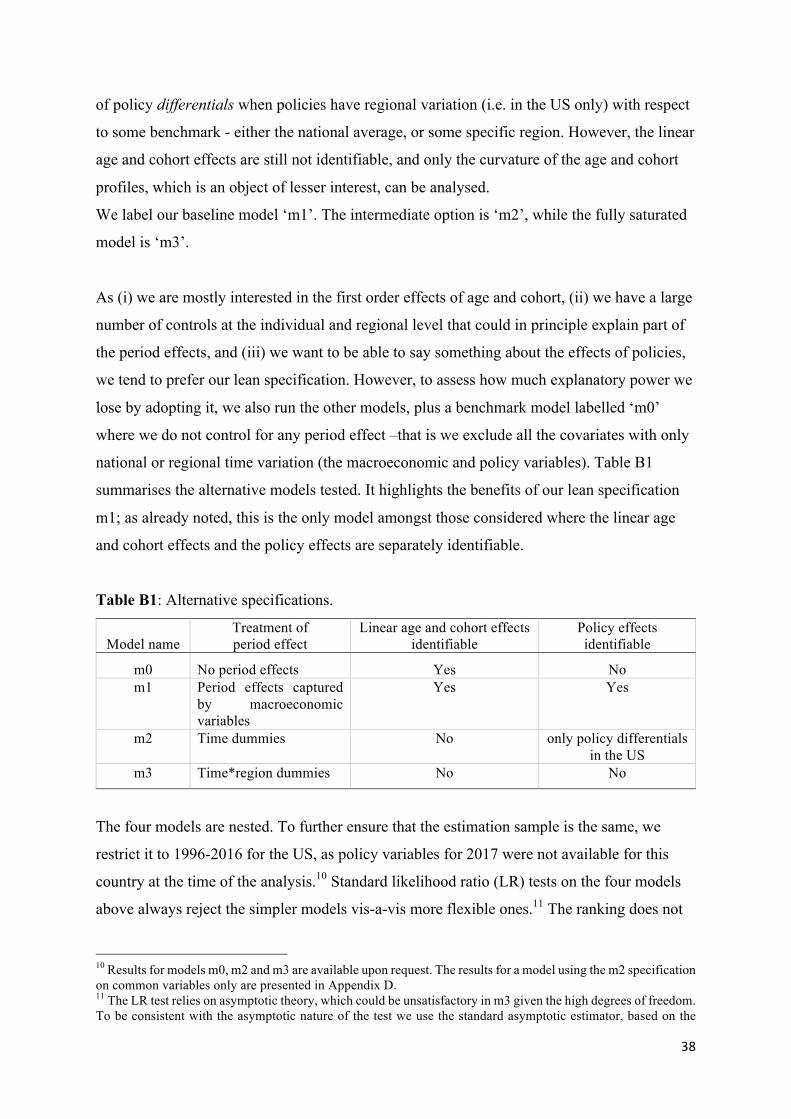
profiles, which is an object of lesser interest, can be analysed.

We label our baseline model ‘m1’. The intermediate option is ‘m2’, while the fully saturated

model is ‘m3’.

As (i) we are mostly interested in the first order effects of age and cohort, (ii) we have a large

number of controls at the individual and regional level that could in principle explain part of

the period effects, and (iii) we want to be able to say something about the effects of policies,

we tend to prefer our lean specification. However, to assess how much explanatory power we

lose by adopting it, we also run the other models, plus a benchmark model labelled ‘m0’

where we do not control for any period effect –that is we exclude all the covariates with only

national or regional time variation (the macroeconomic and policy variables). Table B1

summarises the alternative models tested. It highlights the benefits of our lean specification

m1; as already noted, this is the only model amongst those considered where the linear age

and cohort effects and the policy effects are separately identifiable.

Table B1: Alternative specifications.

Model name Treatment of period effect

Linear age and cohort effects identifiable

Policy effects identifiable

m0 No period effects Yes No m1 Period effects captured

by macroeconomic variables

Yes Yes

m2 Time dummies No only policy differentials in the US

m3 Time*region dummies No No

The four models are nested. To further ensure that the estimation sample is the same, we

restrict it to 1996-2016 for the US, as policy variables for 2017 were not available for this

country at the time of the analysis.10 Standard likelihood ratio (LR) tests on the four models

above always reject the simpler models vis-a-vis more flexible ones.11 The ranking does not

10 Results for models m0, m2 and m3 are available upon request. The results for a model using the m2 specification on common variables only are presented in Appendix D. 11 The LR test relies on asymptotic theory, which could be unsatisfactory in m3 given the high degrees of freedom. To be consistent with the asymptotic nature of the test we use the standard asymptotic estimator, based on the

39

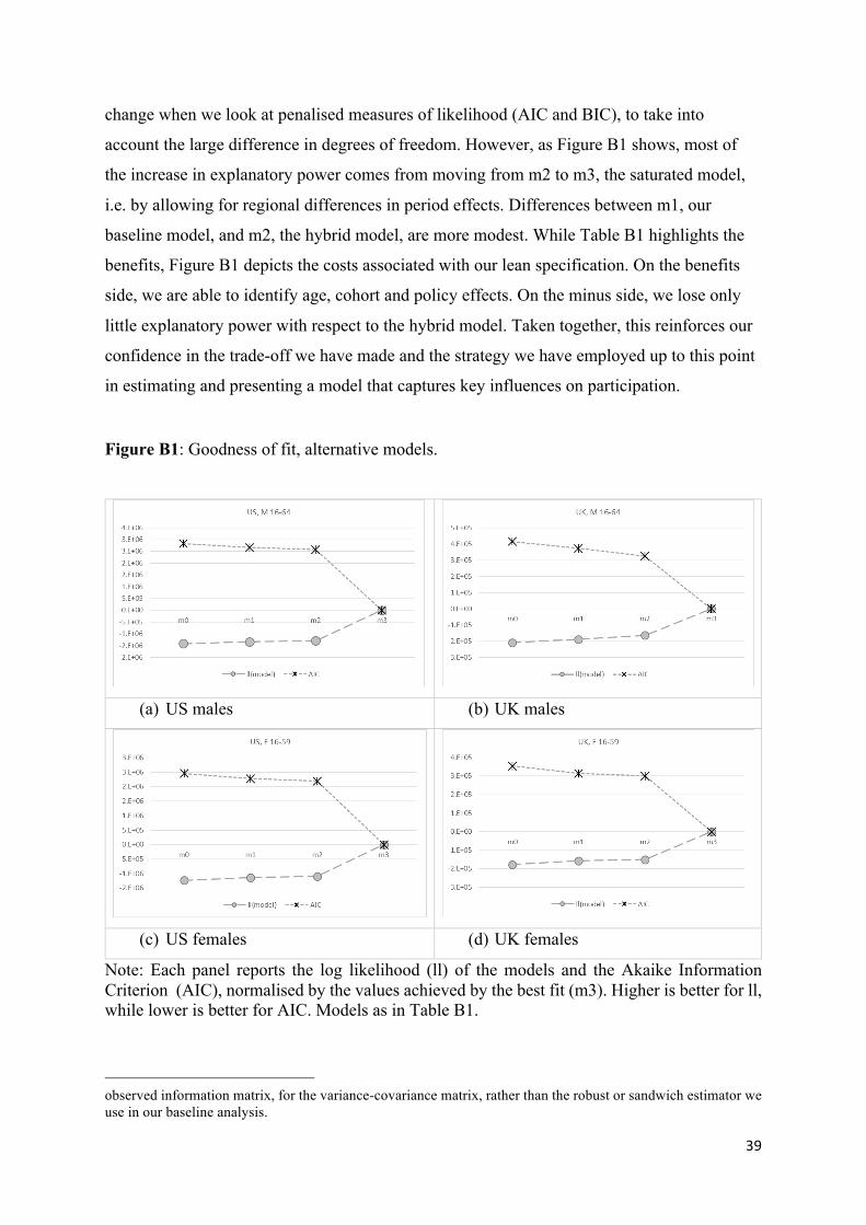
change when we look at penalised measures of likelihood (AIC and BIC), to take into

account the large difference in degrees of freedom. However, as Figure B1 shows, most of

the increase in explanatory power comes from moving from m2 to m3, the saturated model,

i.e. by allowing for regional differences in period effects. Differences between m1, our

baseline model, and m2, the hybrid model, are more modest. While Table B1 highlights the

benefits, Figure B1 depicts the costs associated with our lean specification. On the benefits

side, we are able to identify age, cohort and policy effects. On the minus side, we lose only

little explanatory power with respect to the hybrid model. Taken together, this reinforces our

confidence in the trade-off we have made and the strategy we have employed up to this point

in estimating and presenting a model that captures key influences on participation.

Figure B1: Goodness of fit, alternative models.

(a) US males (b) UK males

(c) US females (d) UK females

Note: Each panel reports the log likelihood (ll) of the models and the Akaike Information Criterion (AIC), normalised by the values achieved by the best fit (m3). Higher is better for ll, while lower is better for AIC. Models as in Table B1.

observed information matrix, for the variance-covariance matrix, rather than the robust or sandwich estimator we use in our baseline analysis.

40

Appendix C

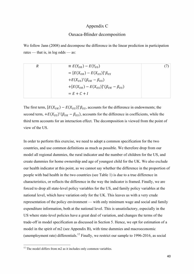
Oaxaca-Blinder decomposition We follow Jann (2008) and decompose the difference in the linear prediction in participation

rates — that is, in log odds — as:

( ≡ * +,- − * +,/ = * 1,- − * 1,/ 23,/+* 1,/ 2 3,- − 3,/ + * 1,- − * 1,/ 2 3,- − 3,/ = * + 5 + 6

(7)

The first term, * 1,- − * 1,/ 23,/, accounts for the difference in endowments; the

second term, +* 1,/ 2 3,- − 3,/ , accounts for the difference in coefficients, while the

third term accounts for an interaction effect. The decomposition is viewed from the point of

view of the US.

In order to perform this exercise, we need to adopt a common specification for the two

countries, and use common definitions as much as possible. We therefore drop from our

model all regional dummies, the rural indicator and the number of children for the US, and

create dummies for home ownership and age of youngest child for the UK. We also exclude

our health indicator at this point, as we cannot say whether the difference in the proportion of

people with bad health in the two countries (see Table 1) is due to a true difference in

characteristics, or reflects the difference in the way the indicator is framed. Finally, we are

forced to drop all state-level policy variables for the US, and family policy variables at the

national level, which have variation only for the UK. This leaves us with a very crude

representation of the policy environment — with only minimum wage and social and family

expenditure information, both at the national level. This is unsatisfactory, especially in the

US where state-level policies have a great deal of variation, and changes the terms of the

trade-off in model specification as discussed in Section 5. Hence, we opt for estimation of a

model in the spirit of m2 (see Appendix B), with time dummies and macroeconomic

(unemployment rate) differentials.12 Finally, we restrict our sample to 1996-2016, as social

12 The model differs from m2 as it includes only common variables.

41

expenditure variables for 2017 are not available (at the moment of writing) for the US. To see

whether the importance of covariates and coefficients has changed over time, we estimate the

model separately for the two sub-periods 1996-2007 and 2008-2017. (The estimation results

for this common specification are reported in Appendix D.)

Table C1a presents the results of the Oaxaca-Blinder decomposition for men, showing for

each sub-period the contribution of endowments, coefficients, and interaction between them

to the estimated difference in participation rates between the UK and the US. Between 1996

and 2007, there was almost no average participation gap between the two countries, with the

participation rate being a mere 0.14 percentage points higher. We see that composition effects

work to lower the participation gap from a US perspective — in other words, “endowments”

of the working-age population are more positive for participation there, so that predicted

participation on that basis would be higher. This is almost exactly offset by negative

behavioural effects (“coefficients”), however, which serve to widen the participation gap

from a US perspective. These two offsetting effects underpin the almost identical levels of

participation observed.

For the 2008-2017 period, by contrast, the average participation gap had become substantial,

with participation more than 3 percentage points higher in the UK. This reflects the fact that

the positive effect of endowments for the US (in reducing this gap) fell markedly over time to

effectively disappear, while the negative effect of coefficients (in widening the gap) also

increased substantially over time (from 1.8 to 3.9 percentage points). Assuming interaction

effects are equally attributable to both endowments and coefficients, endowments account for

46% of the overall deterioration in male participation rates, while coefficients account for the

remaining 54%.

When looking at the importance of each covariate in the bottom part of the table, we must

bear in mind that the effects of age, cohort, and period, given the inclusion of time dummies,

are identified only up to a constant (which can be arbitrarily added to either age, cohort, or

any combination of the two, or attributed to the dummy for the reference year). We therefore

group together the three effects, which also include the effects of policies, under the heading

‘APC’. The main explanation for why composition effects were favourable to the US in the

first sub-period, but became negligible in the second sub-period, relates to the education

profile of the working-age population. The US started with a lower share of individuals with

42

low education but the UK reduce this share faster, so that the two shares converged over time

(as documented in Table D2 below). As far as the effects of behavioural are concerned, the

fact that these turned increasingly against the US reflects a turnaround with respect to the

likelihood of participation for married men, which reduced the gap in the earlier period but

widened it in the later one, together with a reduction in the containment effect of age, period

(including policies), and cohort, and a variety of small changes in the contribution of other

coefficients. Changes in the effect of high education on participation, on the other hand,

served to reduce that gap. The lower impact of home ownership on the propensity to

participate in the US had a large effect on the participation gap throughout, but did not

change substantially between the two periods.

The corresponding results for females are shown in Table C1b. In the 1996-2007 period the

average participation gap was again small, at only 0.17 percentage points. By 2008-2017, the

average gap had become even larger than for males, at 4.5 percentage points. The effect of

endowments on the gap declined substantially between the two time-periods, reducing the

gap from a US perspective by 4 percentage points in the earlier period but only 1 percentage

point by 2008-2017. In the earlier period US women had an even greater advantage over their

UK counterparts than men in terms of employment-related characteristics; by the latter period

this had fallen by three-quarters though not disappeared. As for men, the causes of the overall

deterioration in female participation rates are roughly equally split between endowments

(again, 46%) and coefficients (54%). Similar to men, the main contributory factor is the

spectacular reduction in the fraction of working-age individuals with low education in the

UK, shown in Table C2. However, the increase in the fraction of high-educated individuals in

the UK, which is stronger for females than for males as that table illustrates, also played a

role. The effect of coefficients in widening the participation gap for women also increased

markedly over time, doubling from 3.3 to 6.61 percentage points; this is mainly due to a

change in the overall effect of age, period (including policies) and cohort, which reduced the

participation gap in the first period, and increased it in the second period.

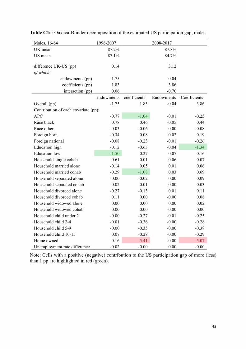
43

Table C1a: Oaxaca-Blinder decomposition of the estimated US participation gap, males.

Males, 16-64 1996-2007 2008-2017 UK mean 87.2% 87.8% US mean 87.1% 84.7%

difference UK-US (pp)

0.14

3.12 of which:

endowments (pp) -1.75 -0.04 coefficients (pp) 1.83 3.86 interaction (pp) 0.06 -0.70

endowments coefficients Endowments Coefficients Overall (pp) -1.75 1.83 -0.04 3.86 Contribution of each covariate (pp): APC -0.77 -1.04 -0.01 -0.25 Race black 0.78 0.46 -0.05 0.44 Race other 0.03 -0.06 0.00 -0.08 Foreign born -0.34 0.08 0.02 0.19 Foreign national -0.08 -0.23 -0.01 -0.26 Education high -0.12 -0.63 -0.04 -1.34 Education low -1.50 0.27 0.07 0.16 Household single cohab 0.61 0.01 -0.06 0.07 Household married alone -0.14 0.05 0.01 0.06 Household married cohab -0.29 -1.08 0.03 0.69 Household separated alone -0.00 -0.02 -0.00 0.09 Household separated cohab 0.02 0.01 -0.00 0.03 Household divorced alone -0.27 -0.13 0.01 0.11 Household divorced cohab 0.11 0.00 -0.00 0.08 Household widowed alone 0.00 0.00 0.00 0.02 Household widowed cohab 0.00 0.00 -0.00 0.00 Household child under 2 -0.00 -0.27 -0.01 -0.25 Household child 2-4 -0.01 -0.36 -0.00 -0.28 Household child 5-9 -0.00 -0.35 -0.00 -0.38 Household child 10-15 0.07 -0.28 -0.00 -0.29 Home owned 0.16 5.41 -0.00 5.07 Unemployment rate difference -0.02 -0.00 0.00 -0.00

Note: Cells with a positive (negative) contribution to the US participation gap of more (less) than 1 pp are highlighted in red (green).

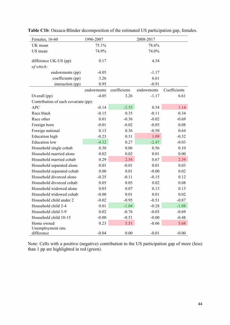
44

Table C1b: Oaxaca-Blinder decomposition of the estimated US participation gap, females.

Females, 16-60 1996-2007 2008-2017 UK mean 75.1% 78.6% US mean 74.9% 74.0%

difference UK-US (pp)

0.17

4.54 of which:

endowments (pp) -4.05 -1.17 coefficients (pp) 3.26 6.61 interaction (pp) 0.95 -0.91

endowments coefficients endowments Coefficients Overall (pp) -4.05 3.26 -1.17 6.61 Contribution of each covariate (pp): APC -0.14 -2.55 0.54 1.14 Race black -0.15 0.35 -0.11 0.34 Race other 0.01 -0.36 -0.02 -0.69 Foreign born -0.01 -0.02 -0.05 0.08 Foreign national 0.13 0.36 -0.50 0.64 Education high -0.23 0.31 1.09 -0.32 Education low -4.32 0.27 -2.47 -0.03 Household single cohab 0.30 0.06 0.56 0.10 Household married alone 0.02 0.02 0.01 0.00 Household married cohab 0.29 2.54 0.67 2.39 Household separated alone 0.01 -0.01 0.01 0.03 Household separated cohab 0.00 0.01 -0.00 0.02 Household divorced alone -0.25 -0.11 -0.15 0.12 Household divorced cohab 0.05 0.05 0.02 0.08 Household widowed alone 0.03 0.07 0.13 0.13 Household widowed cohab -0.00 0.01 0.01 0.02 Household child under 2 -0.02 -0.95 -0.51 -0.87 Household child 2-4 0.01 -1.04 -0.28 -1.08 Household child 5-9 0.02 -0.76 -0.03 -0.69 Household child 10-15 -0.00 -0.51 -0.00 -0.48 Home owned 0.23 5.51 -0.06 5.68 Unemployment rate difference -0.04 0.00 -0.01 -0.00

Note: Cells with a positive (negative) contribution to the US participation gap of more (less) than 1 pp are highlighted in red (green).

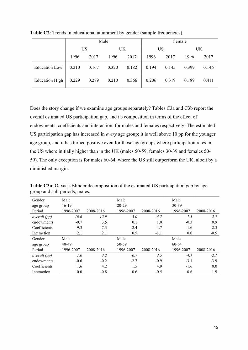
45

Table C2: Trends in educational attainment by gender (sample frequencies).

Male Female

US UK US UK

1996 2017 1996 2017 1996 2017 1996 2017

Education Low 0.210 0.167 0.320 0.182 0.194 0.145 0.399 0.146

Education High 0.229 0.279 0.210 0.366 0.206 0.319 0.189 0.411

Does the story change if we examine age groups separately? Tables C3a and C3b report the

overall estimated US participation gap, and its composition in terms of the effect of

endowments, coefficients and interaction, for males and females respectively. The estimated

US participation gap has increased in every age group; it is well above 10 pp for the younger

age group, and it has turned positive even for those age groups where participation rates in

the US where initially higher than in the UK (males 50-59, females 30-39 and females 50-

59). The only exception is for males 60-64, where the US still outperform the UK, albeit by a

diminished margin.

Table C3a: Oaxaca-Blinder decomposition of the estimated US participation gap by age group and sub-periods, males.

Gender Male Male Male age group 16-19 20-29 30-39 Period 1996-2007 2008-2016 1996-2007 2008-2016 1996-2007 2008-2016 overall (pp) 10.6 12.9 3.0 4.7 1.3 2.7 endowments -0.7 3.5 0.1 1.0 -0.3 0.9 Coefficients 9.3 7.3 2.4 4.7 1.6 2.3 Interaction 2.1 2.1 0.5 -1.1 0.0 -0.5 Gender Male Male Male age group 40-49 50-59 60-64 Period 1996-2007 2008-2016 1996-2007 2008-2016 1996-2007 2008-2016 overall (pp) 1.0 3.2 -0.7 3.5 -4.1 -2.1 endowments -0.6 -0.2 -2.7 -0.9 -3.1 -3.9 Coefficients 1.6 4.2 1.5 4.9 -1.6 0.0 Interaction 0.0 -0.8 0.6 -0.5 0.6 1.9

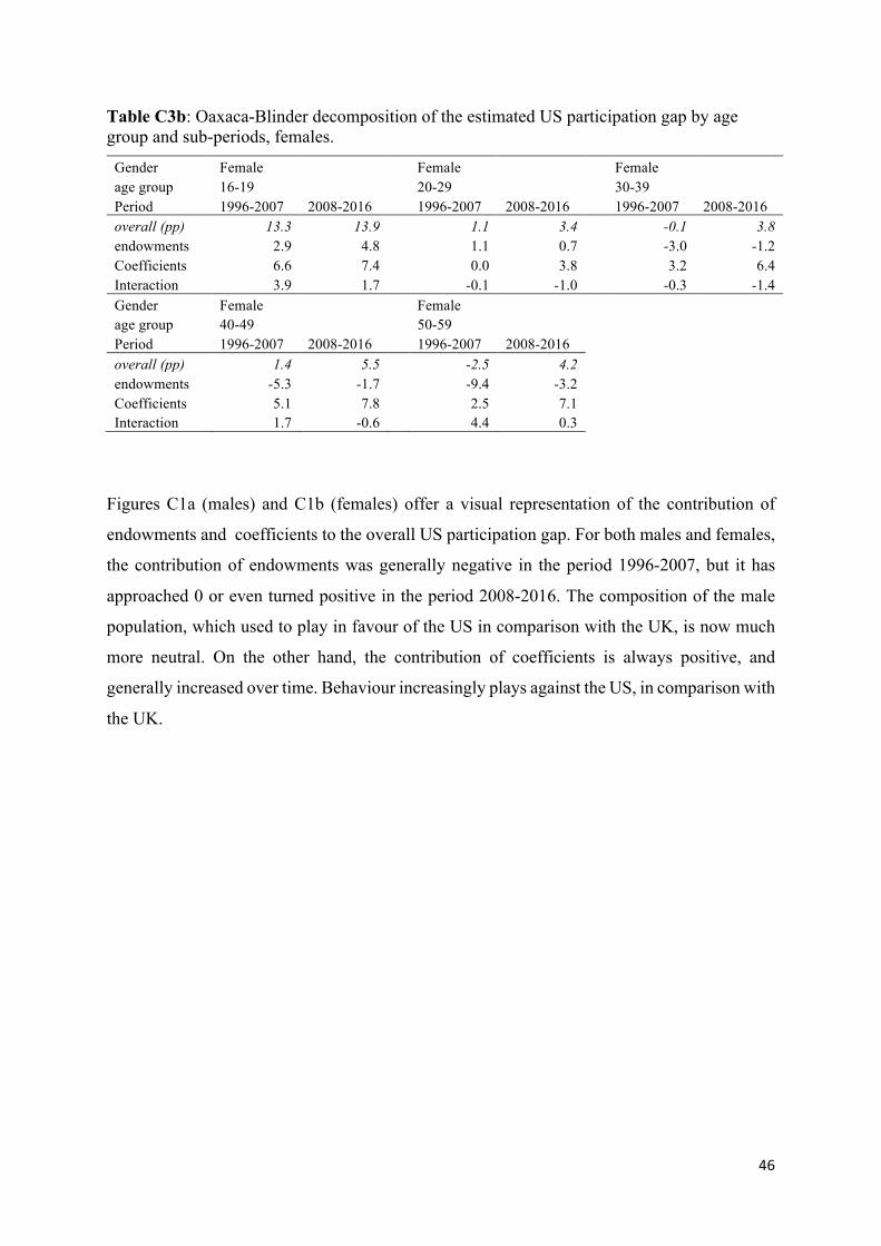
46

Table C3b: Oaxaca-Blinder decomposition of the estimated US participation gap by age group and sub-periods, females.

Gender Female Female Female age group 16-19 20-29 30-39 Period 1996-2007 2008-2016 1996-2007 2008-2016 1996-2007 2008-2016 overall (pp) 13.3 13.9 1.1 3.4 -0.1 3.8 endowments 2.9 4.8 1.1 0.7 -3.0 -1.2 Coefficients 6.6 7.4 0.0 3.8 3.2 6.4 Interaction 3.9 1.7 -0.1 -1.0 -0.3 -1.4 Gender Female Female age group 40-49 50-59 Period 1996-2007 2008-2016 1996-2007 2008-2016 overall (pp) 1.4 5.5 -2.5 4.2 endowments -5.3 -1.7 -9.4 -3.2 Coefficients 5.1 7.8 2.5 7.1 Interaction 1.7 -0.6 4.4 0.3

Figures C1a (males) and C1b (females) offer a visual representation of the contribution of

endowments and coefficients to the overall US participation gap. For both males and females,

the contribution of endowments was generally negative in the period 1996-2007, but it has

approached 0 or even turned positive in the period 2008-2016. The composition of the male

population, which used to play in favour of the US in comparison with the UK, is now much

more neutral. On the other hand, the contribution of coefficients is always positive, and

generally increased over time. Behaviour increasingly plays against the US, in comparison with

the UK.

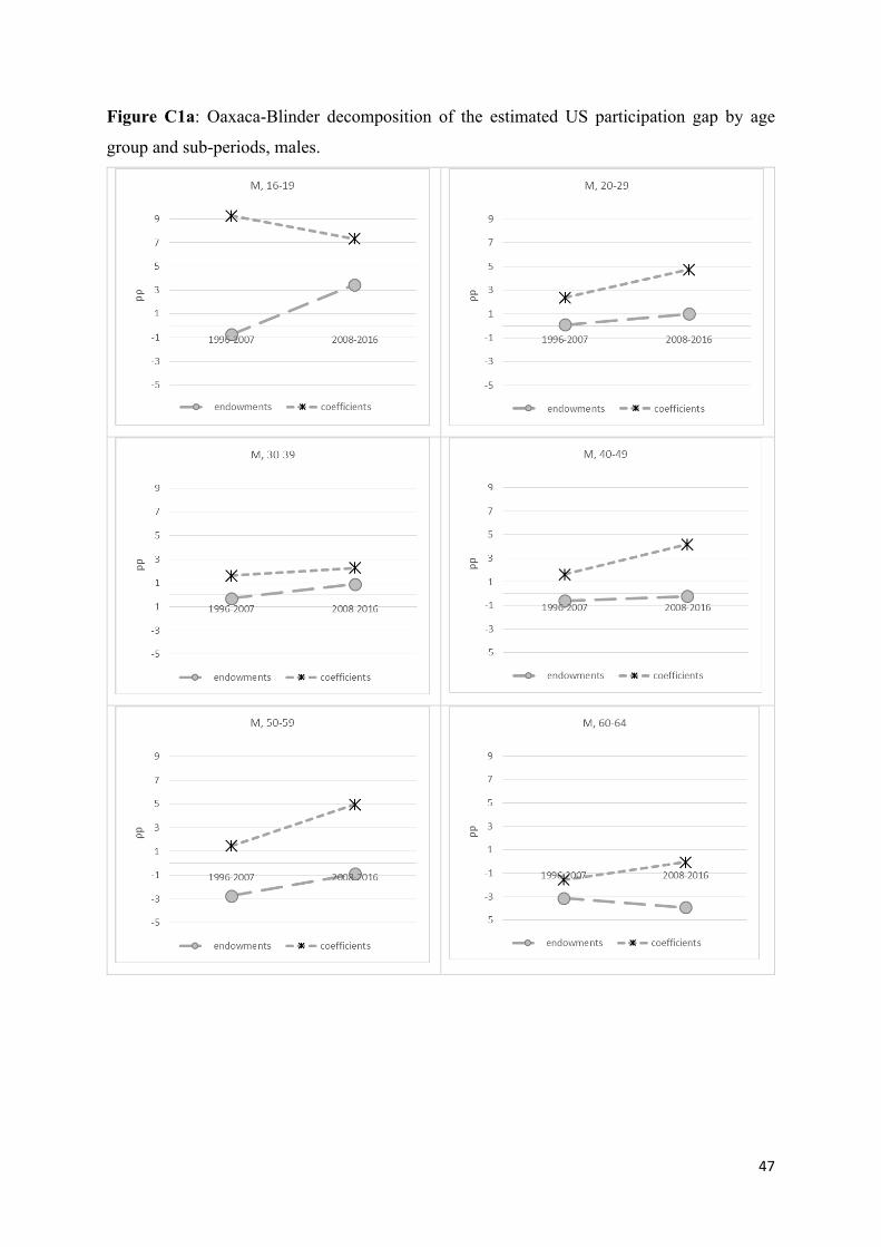
47

Figure C1a: Oaxaca-Blinder decomposition of the estimated US participation gap by age

group and sub-periods, males.

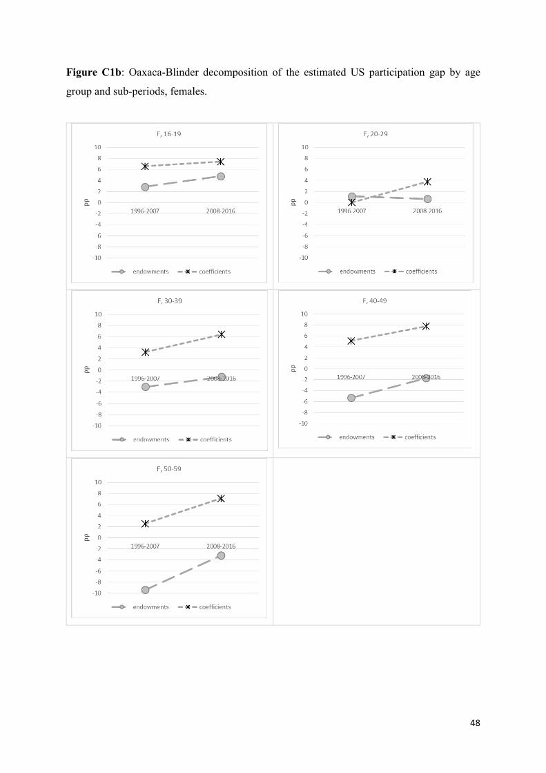
48

Figure C1b: Oaxaca-Blinder decomposition of the estimated US participation gap by age

group and sub-periods, females.

49

Appendix D

Estimated Participation Model with Common Specification

Table D1: Logit estimates of the probability of being in the labour force, common specification, males. Students excluded.

(1) (2) (3) (4) US UK US UK M 16-64 M 16-64 M 16-64 M 16-64 VARIABLES 1996-2007 1996-2007 2008-2017 2008-2017 Age 0.094 *** 0.066 *** 0.123 *** 0.154 *** Age squared -0.002 *** -0.002 *** -0.002 *** -0.003 *** Year of birth 0.038 *** 0.087 *** 0.007 0.022 ** Year of birth squared 0.000 *** -0.001 *** 0.000 0.000 *** Race black -0.583 *** -0.072 -0.480 *** -0.058 Race other -0.492 *** -0.619 *** -0.376 *** -0.489 *** Foreign born 0.347 *** 0.408 *** 0.442 *** 0.556 *** Foreign national 0.189 *** -0.099 *** 0.352 *** 0.067 ** Education high -13.91 6.15 -34.72 *** 22.41 * Education low -25.92 *** 13.19 ** -2.11 35.67 *** Year x education high 0.007 * -0.003 0.018 *** -0.011 * Year x education low 0.013 *** -0.007 ** 0.001 -0.018 *** Household single cohab 0.764 *** 0.817 *** 0.758 *** 0.934 *** Household married alone 0.766 *** 1.150 *** 0.772 *** 1.253 *** Household married cohab 1.115 *** 0.884 *** 0.941 *** 1.085 *** Household separated alone 0.529 *** 0.387 *** 0.263 *** 0.758 *** Household separated cohab 0.670 *** 1.358 *** 0.454 *** 1.513 *** Household divorced alone 0.512 *** 0.310 *** 0.387 *** 0.547 *** Household divorced cohab 0.953 *** 0.965 *** 0.694 *** 1.152 *** Household widowed alone 0.267 *** 0.289 *** 0.072 0.359 *** Household widowed cohab 0.455 *** 0.775 *** 0.323 ** 0.925 *** Household child2 0.252 *** -0.235 *** 0.351 *** -0.120 *** Household child4 0.290 *** -0.298 *** 0.288 *** -0.178 *** Household child9 0.270 *** -0.206 *** 0.388 *** -0.126 *** Household child15 0.349 *** -0.024 0.416 *** 0.038 Home owned 0.195 *** 1.176 *** 0.158 *** 1.026 *** Unemployment rate diff -6.934 *** -7.906 *** -3.925 *** -4.687 *** 1996 0.034 -0.105 *** 1997 0.070 ** -0.131 *** 1998 0.063 ** -0.186 *** 1999 0.027 -0.166 *** 2000 0.044 -0.165 *** 2001 0.022 -0.198 *** 2002 0.012 -0.192 *** 2003 -0.045 * -0.122 *** 2004 -0.078 *** -0.148 *** 2005 -0.060 ** -0.139 *** 2006 -0.018 -0.063 ** 2007 2008 0.025 -0.251 *** 2009 -0.032 -0.231 ***

50

2010 -0.017 -0.241 *** 2011 -0.081 *** -0.184 *** 2012 -0.078 *** -0.139 *** 2013 -0.017 -0.106 *** 2014 -0.007 -0.057 * 2015 -0.015 -0.050 2016 0.006 -0.017 Observations 580,515 444,333 530,802 274,084 chi2 144667 159295 118940 95339 P 0.00 0.00 0.00 0.00 Robust standard errors in parentheses *** p<0.01, ** p<0.05, * p<0.1

Note: The baseline is a medium education white individual, single and not cohabiting, who is renting. Cohort is measured subtracting 1,900 from year of birth.

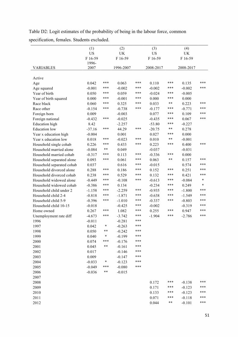
51

Table D2: Logit estimates of the probability of being in the labour force, common

specification, females. Students excluded.

(1) (2) (3) (4) US UK US UK F 16-59 F 16-59 F 16-59 F 16-59

VARIABLES 1996-2007 1996-2007 2008-2017 2008-2017

Active Age 0.042 *** 0.063 *** 0.110 *** 0.135 *** Age squared -0.001 *** -0.002 *** -0.002 *** -0.002 *** Year of birth 0.050 *** 0.059 *** -0.024 *** -0.005 Year of birth squared 0.000 *** -0.001 *** 0.000 *** 0.000 Race black 0.060 *** 0.325 *** 0.033 ** 0.223 *** Race other -0.154 *** -0.738 *** -0.177 *** -0.771 *** Foreign born 0.009 -0.003 0.077 *** 0.109 *** Foreign national -0.432 *** -0.025 -0.435 *** 0.067 *** Education high 8.42 -2.257 -53.80 *** -0.227 Education low -37.16 *** 44.29 *** -20.75 ** 0.278 Year x education high -0.004 0.001 0.027 *** 0.000 Year x education low 0.018 *** -0.023 *** 0.010 ** -0.001 Household single cohab 0.226 *** 0.433 *** 0.223 *** 0.400 *** Household married alone -0.084 ** 0.049 -0.037 -0.031 Household married cohab -0.317 *** 0.113 *** -0.336 *** 0.000 Household separated alone 0.093 *** 0.061 *** 0.063 ** 0.157 *** Household separated cohab 0.037 0.616 *** -0.015 0.574 *** Household divorced alone 0.288 *** 0.186 *** 0.152 *** 0.251 *** Household divorced cohab 0.238 *** 0.529 *** 0.132 *** 0.421 *** Household widowed alone -0.449 *** -0.108 *** -0.613 *** -0.084 * Household widowed cohab -0.386 *** 0.134 -0.234 *** 0.249 * Household child under 2 -1.158 *** -2.259 *** -0.935 *** -1.800 *** Household child 2-4 -0.818 *** -1.871 *** -0.638 *** -1.549 *** Household child 5-9 -0.396 *** -1.010 *** -0.337 *** -0.803 *** Household child 10-15 -0.018 -0.425 *** -0.002 -0.319 *** Home owned 0.267 *** 1.082 *** 0.255 *** 0.947 *** Unemployment rate diff -4.673 *** -3.742 *** -1.904 *** -2.786 *** 1996 -0.011 -0.281 *** 1997 0.042 * -0.263 *** 1998 0.050 ** -0.242 *** 1999 0.040 * -0.199 *** 2000 0.074 *** -0.176 *** 2001 0.045 ** -0.161 *** 2002 0.017 -0.146 *** 2003 0.009 -0.147 *** 2004 -0.033 * -0.123 *** 2005 -0.049 *** -0.080 *** 2006 -0.036 ** -0.015 2007 2008 0.172 *** -0.138 *** 2009 0.171 *** -0.123 *** 2010 0.133 *** -0.123 *** 2011 0.071 *** -0.118 *** 2012 0.044 ** -0.101 ***

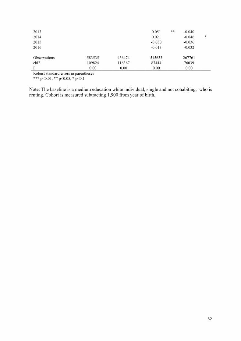
52

2013 0.051 ** -0.040 2014 0.021 -0.046 * 2015 -0.030 -0.036 2016 -0.013 -0.032 Observations 583535 436474 515633 267761 chi2 109824 116367 87444 76039 P 0.00 0.00 0.00 0.00 Robust standard errors in parentheses *** p<0.01, ** p<0.05, * p<0.1

Note: The baseline is a medium education white individual, single and not cohabiting, who is renting. Cohort is measured subtracting 1,900 from year of birth.