What Explains Inflation in China?

A Research Paper presented by:

Yuhua ZHANG

Singapore

in partial fulfillment of the requirements for obtaining the degree of

MASTER OF ARTS IN DEVELOPMENT STUDIES

Major:

Economics of Development

(ECD)

Specialization: Econometric Analysis of Development Policies

Members of the Examining Committee:

Dr. Howard Nicholas (Supervisor)

Dr. Peter van Bergeijk (Reader)

The Hague, The Netherlands

December 2016

ii

i

Contents

Chapter 1: Introduction ............................................................................................................................. 1

I. Significance of the Study ....................................................................................................................... 2

II. Research Objectives and Questions ..................................................................................................... 2

III. Hypothesis and Methodology ............................................................................................................. 3

IV. Scope and Limitations ........................................................................................................................ 3

V. Structure of the Paper ........................................................................................................................... 4

Chapter 2: Background of the Study ........................................................................................................ 5

I. Definition of Inflation ............................................................................................................................ 5

II. Measurement of Inflation ..................................................................................................................... 6

1. Consumer Price Index ....................................................................................................................... 6

2. Retail Price Index .............................................................................................................................. 7

3. Producer Price Index ......................................................................................................................... 7

4. GDP Deflator .................................................................................................................................... 7

5. Comparison of Inflation Measures .................................................................................................... 8

III. Policy Factors Related with Inflation in China ................................................................................... 8

1. Price Control ..................................................................................................................................... 9

2. Wage Control .................................................................................................................................... 9

3. Inflation Target ................................................................................................................................. 9

IV. Evolution of Inflation in China ......................................................................................................... 10

Period 1: 1981 to 1997 (Figure 2) ....................................................................................................... 10

Period 2: 1998 to 2014 (Figure 3) ....................................................................................................... 12

Chapter 3: Major Theories on Inflation ................................................................................................. 14

I. Quantity Theory of Money .................................................................................................................. 14

1. The Empirical Model ...................................................................................................................... 16

2. Assumptions .................................................................................................................................... 19

3. Applications in China...................................................................................................................... 19

The Impotence of Quantity Theory of Money in Recent Years .......................................................... 20

II. New Keynesian Phillips Curve........................................................................................................... 21

1. The Empirical Model ...................................................................................................................... 23

2. Assumptions .................................................................................................................................... 25

3. Application to China ....................................................................................................................... 26

III. Structural Cost-push Theory ............................................................................................................. 27

1. The Empirical Model ...................................................................................................................... 29

ii

2. Assumptions .................................................................................................................................... 30

3. Application in China ....................................................................................................................... 30

IV. Summary ........................................................................................................................................... 31

Chapter 4: Econometric Analysis ............................................................................................................ 32

I. Summary of Variables ......................................................................................................................... 32

II. Stationarity of Variables ..................................................................................................................... 34

III. Econometric Results ......................................................................................................................... 36

1. Quantity Theory of Money ............................................................................................................. 37

2. New Keynesian Phillips Curve ....................................................................................................... 41

3. Structuralist Cost-push Theory ....................................................................................................... 45

IV. Summary ........................................................................................................................................... 49

Chapter 5: Conclusion .............................................................................................................................. 50

References .................................................................................................................................................. 52

iii

List of Tables

Table 1 China's CPI Categories and Composition ........................................................................................ 6

Table 2 Description of Variables ................................................................................................................ 33

Table 3 Stationarity of Variables ................................................................................................................ 35

Table 4 OLS Results of the Quantity Theory of Money ............................................................................. 39

Table 5 VAR Results of the Quantity Theory of Money ............................................................................ 40

Table 6 OLS Results of the New Keynesian Phillips Curve ....................................................................... 42

Table 7 VAR Results of the New Keynesian Phillips Curve ...................................................................... 43

Table 8 OLS Results of the Structuralist Cost-push Theory – Primary Results on infc ............................. 47

Table 9 OLS Results of the Structuralist Cost-push Theory – Robustness Check on infgdpd ................... 48

List of Figures

Figure 1 Inflation in China in Different Measures ........................................................................................ 8

Figure 2 Evolution of Inflation 1981-1997 ................................................................................................. 10

Figure 3 Evolution of Inflation 1998-2014 ................................................................................................. 12

Figure 4 The long-run Quantity Theory of Money ..................................................................................... 16

Figure 5 Velocity and Nominal Interest Rate in China ............................................................................... 18

Figure 6 Residential Property Price (left) and Share Price (right), Quarterly, Index 2010=100 ................ 21

Figure 7 Short-run and Long-run Phillips Curve ........................................................................................ 22

Figure 8 Structural Cost-push Theory of Inflation ...................................................................................... 29

Figure 9 Autocorrelation of Inflation by CPI and GDP Deflator ................................................................ 36

Figure 10 Graphic Depiction of Inflation and Excess Money Supply ........................................................ 38

Figure 11 Stability of the VAR Models - Quantity Theory of Money ........................................................ 41

Figure 12 Stability of the Models - New Keynesian Phillips Curve ........................................................... 44

Figure 13 Graphic Depiction of the Evolution of Structural Cost-push Variables ..................................... 45

Figure 14 Inflation and Food Price Indices ................................................................................................. 48

iv

List of Acronyms

CPI Consumer Price Index

GDP Gross Domestic Product

IMF International Monetary Fund

M0 Cash Base

M1 Narrow Money

M2 Broad Money

NAIRU Non-Accelerating Inflation Rate of Unemployment

NBS China National Bureau of Statistics

OLS Ordinary Least Squares

OECD Organisation for Economic Cooperation and Development

PBOC People’s Bank of China

PPI Producer Price Index

RMB Renminbi

RPI Retail Price Index

VAR Vector Auto-regression Model

WTO World Trade Organization

v

Abstract

This paper studied China’s inflation based on yearly data of related factors in the past three decades. It

examined the nature and causes of inflation evolution in China. The findings indicated that from demand

pull perspective, the Quantity Theory of Money offers a sensible explanation of inflation trends in China

than the New Keynesian Phillips Curve; and from cost push perspective, the Structuralist Cost-push

Theory correlates the food price movement with inflation trend. The year 1998 seems to be a structural

break in inflation evolution. Overall, the paper confirmed the hypothesis that inflation in China is largely

driven by excess money supply, and is correlated with changes in food price level. However, the findings

are subject to various limitations of the paper, such as data quality, econometric technics, and model

sophistication.

Relevance to Development Studies

Development studies in general have a quite broad scope, covering a wide range of topics, from social

and economic topics, to political, environmental, and humanitarian issues. This paper focuses on the

economic phenomenon of inflation in China, which fits well for a development study, because inflation,

and its opposite deflation, are unavoidable reality of economic growth and are important signals to

policymakers. In addition, China is the largest developing country in the world, and its economic growth

path and policies offer imperative examples and lessons to other developing countries. However, given

the complex policy environment in China, it is hard to tell what theories offer a better explanation of

inflation evolution. Therefore, this paper attempts to study and apply different theories in China’s context

and identify a theoretical framework that could explain its inflation trend.

Acknowledgements

This paper has benefited from insightful comments and advice from Dr Howard Nicholas and Dr Peter van Bergeijk. Their valuable feedback and direction are highly appreciated.

Key words

Inflation, monetary policy, Quantity Theory of Money, New Keynesian Phillips Curve, Structural Cost-

push Theory

1

Chapter 1: Introduction

As the global economy becomes increasingly intertwined, managing internal balances and external shocks

poses a great challenge to policy makers. Various policy tools are available, among which monetary

policy is perhaps the most prominent, as it plays the role of steering a stable macro environment and

fending off crises. Across the world, design and implementation of monetary policy exhibit diversity.

The impossible trinity states that no country can enjoy monetary policy independence while having a

stable exchange rate and free capital flows (Obstfeld, et al., 2004). Hence almost all large economies in

the world opt for a flexible or semi-flexible exchange rate, so as to have free movement of capital and

independence of monetary policy. In contrast, China, as an exception, chooses to manage the exchange

rate, which entails capital control and forfeits the independence in monetary policy making (Goldstein &

Lardy, 2007).

Central to current monetary policy in the major advanced economies is price stability, where an increase

in the general price level is termed inflation and a decrease deflation. Inflation and deflation distort price

signals, leading to inefficient allocation of resources; they also undermine the credibility of the central

bank, making it difficult to conduct macroeconomic management. Therefore, major advanced economies

in the world all adopt inflation targeting as the anchor of monetary policy, namely the United States, the

Euro Zone, and Japan. In this regard, China again takes a different path – aiming to achieve price stability,

economic growth and currency stability through targeting monetary aggregates, both M1 and M2 (Pankki,

2015; Geiger, 2008). The Law on People’s Bank of China (PBOC) stipulates that the goal of monetary

policy is to maintain the value of the Renminbi (RMB). This policy setup has created a considerable

burden for China to manage domestic inflation. In addition, although since 2002, China publishes an

inflation target each year, its role is not yet clear on the monetary policy compass (Geiger, 2008).

Typically, to maintain price stability, central banks use both price-based tools, such as interest rate, and

quantity-based tools, such as open market operations1. However, due to the structural transformation of

the economy and underdeveloped domestic banking system, China’s approach to price stability is also

unconventional. On top of the common policy instruments, such as reserve requirements and central bank

1 Instruments that are based on the price of money are price-based tools and quantity-based tools change the amount

of money in the financial system without considering the price of money (Geiger, 2008). It is important to note that

open market operations also impact interest rates through the market.

2

lending rate, the PBOC also adopts uncommon instruments, such as window guidance, credit plans, and

direct PBOC lending to manage the price level2 (Geiger, 2008).

I. Significance of the Study

Since the global financial crisis in 2008, China faces many macroeconomic problems. Internally, the real

estate sector is overheating and financial markets exhibit extensive volatility. Externally, global demand

is weakening and export is turning sluggish. This challenges its traditional monetary policy framework

and forces China to ‘focus on inflation control while supporting transition and reform’ (quoted from

speech of PBOC Governor Zhou Xiaochuan) (Zhou, 2012). Although China wishes to achieve multiple

objectives though monetary policy, ‘keeping inflation at bay has always been the most important mandate

of the central bank’ (Zhou, 2012).

However, to manage inflation in China is not an easy task. The inflexible exchange rate system exposes

China to the risk of importing foreign inflation or deflation, at the same time financially-fragile domestic

banking system undermines PBOC’s ability to adjust the interest rate to head off inflationary or

deflationary pressures (Goodfriend & Prasad, 2011). Against this background, PBOC’s ability to maintain

a low domestic price level is severely restricted. Furthermore, PBOC has been in transition, from applying

more traditional quantity-based tools to more price-based tools.

All these factors make China an interesting case to study inflation. Specifically, what drives the long-term

evolution of inflation phenomenon and whether there is an intrinsic theoretical framework that PBOC

follows when prescribing monetary policies.

II. Research Objectives and Questions

The main research question of this paper is what explains inflation in China. The research paper will

examine the nature and causes of inflation3 in China. By nature, it will look into definition, measurement,

and empirical trends; and by causes, it will examine inflation using theories of three major economic

schools, which are most influential in studying and advising monetary policies. They are the Neoclassical

2 Window guidance is where the central bank uses benevolent compulsion to persuade banks and other financial

institutions to stick to official guidelines. In this way, the central banks put moral pressure on financial players to

make them operate consistently with national needs. Credit plan is to issue necessary credits to reach a given output

targets (Geiger, 2008). 3 As inflation and deflation are two sides of the same coin, in the paper, inflation is mainly used instead of

mentioning both for brevity.

3

Quantity Theory of Money, New Keynesian Philips Curve, and the Structuralist Cost-push Theory. Given

data availability, it will analyze inflation evolution from 1980 onwards.

The study aims to present a case of inflation not only under a regime of managed exchange rate, but also

against the backdrop of major reforms towards a more market-and price-based economic system. It will

identify distinct trends in inflation over different periods of time, investigate the reliability of the price

indices, suggest the implicit view of the PBOC with regards to the causes of inflation, and assess whether

this view is supported by theory and evidence.

The paper will address the following questions through descriptive and econometric analysis:

1. How does China define and measure inflation?

2. How does inflation evolve in China? Are there discernible trends in different periods?

3. What drives the movement of the aggregate money price level in China? Does it change over time?

III. Hypothesis and Methodology

Based on empirical trends of inflation and explanatory factors (discussed substantially in chapter 3), the

hypothesis of this research paper is that inflation in China is largely driven by excess money supply,

and is correlated with changes in food price level. Specifically, from demand pull perspective, the

Quantity Theory of Money appears to be superior than the New Keynesian Philips Curve in explaining

inflation in China; from cost-push perspective, the Structuralist Cost-push also holds explanatory power.

The hypothesis suggests that to manage inflation in the long run, China should consider both demand pull

and cost push theories.

This research paper conducts explorative data analysis and econometric investigation based on secondary

data. The paper examines literature in different theoretical approaches for calculation and description of

inflation. Given limited access to China’s data, the paper complements data from the National Statistical

Bureau (NBS) with international databases, such as IMF data, WTO Stats, and the World Development

Indicators, etc. The main econometric technic is the ordinary least squares (OLS), and vector auto-

regression model (VAR) is also used wherever there is enough data.

IV. Scope and Limitations

The focus of this paper is theories and factors that explain the causes of inflation in China’s context.

Although it draws on related policies for discussion, the paper will not review and assess the monetary

4

policies conducted by PBOC, and will only consider them to explain inflation4. Nor will the paper

examine the impact of inflation on broader economic growth in China.

Theories on inflation are complex, contentious, and constantly evolving. The paper aims to establish a

broad and basic understanding of the inflation evolution in China, hence it attempts to test data on the

fundamentals of three major theories rather than one single theory. This incurs a sacrifice of depth to

breadth. Papers with one theory usually discuss the evolution and application of the theory in an

exhaustive way. This paper focuses on applying fundamentals of the three theories in China’s context;

hence it is not aimed at presenting all the possible models and development of these theories, nor is it

aimed at interrogating these theories and identifying their inapplicability.

Lastly, data availability and quality impose constraints on the analysis. China’s official statistics have

long been questioned for its reliability. Nakamura et al. found that official data in China are smoothed to

reduce the spikes and troughs, which leads to misperception of the economic reality (Nakamura, et al.,

2015). Because of this, Premier of China, Li Keqiang, once spoke that ‘electricity consumption, rail cargo

volume and bank lending’ are more accurate indicators of economic activities (Reuters, cited in

Nakamura, et al., 2015, p115). In addition, China has gone through sweeping reforms in the past decades,

which affected the stability of definitions and measurement of macroeconomic indicators, denting

comparability and quality of data (Mehrotra, et al., 2007). For example, China used different indices to

measure inflation in the studied period.

V. Structure of the Paper

The paper consists of five chapters. Chapter 1 is introduction. Chapter 2 presents the background of this

study, covering the definition and measurement of inflation, the policy factors, and a discussion on the

evolution of inflation in China. Chapter 3 reviews the previous literatures on theoretical frameworks and

respective applications in China. Chapter 4 of the paper is the descriptive analysis, and the econometric

models to test the hypothesis. The last chapter is conclusion.

4 Research on inflation and monetary policy always faces the issue of reverse causality, as monetary policy is

usually used to address inflation/deflation, while inflation/deflation can be a consequence of monetary policy.

5

Chapter 2: Background of the Study

This chapter presents the background of the study. As countries use different methodologies in calculating

inflation indices, this chapter starts with the definition and measurement of inflation in China, followed

by a discussion of policy factors that directly impact on measurement. The last subsection describes the

evolution of inflation in China.

I. Definition of Inflation

Inflation, in general, refers to ‘the rate of increase in prices over a given period of time’; it reflects ‘how

much more expensive a set of goods and services has become over a certain period, usually a year’ (Oner,

2012). Closely linked with inflation are concepts of deflation, disinflation and stagflation. Deflation is the

antonym of inflation, denoting the sustained decline of prices over a specific period. Disinflation,

opposite of inflation, is termed as the reduction of rate of inflation or a temporary decrease in the general

price level in an economy (Banque de France, 2009). Stagflation is a special case of inflation; it applies to

the economic condition under which high inflation is combined with economic stagnation and high

unemployment (Gregory, 2009).

Conventionally, moderate inflation is in the range of 1 to 20 percent per year, with below 5 percent

termed as creeping inflation and above 5 percent termed as trotting inflation. When inflation goes beyond

20 percent, it is called galloping inflation; and beyond 1000 percent, it is called hyper-inflation. In

addition, headline inflation and core inflation are also common terms, referring to price level of all items

and price level excluding food and energy respectively5 (Haberler, 1960).

According to the China National Bureau of Statistics (NBS), inflation refers to a monetary phenomenon

where money supply exceeds money demand, hence the currency devaluates (China National Bureau of

Statistics, 2011). It is shown as a situation where the general price level of a basket of commodities and

services for household consumption rises persistently in a non-random and lasting fashion. It is neither

the price rise of stocks, bonds, or other financial assets, nor the price rise of a specific product or service,

nor the price rise in a certain region only. In early times, Chinese government deemed excessive money

supply as the only cause of inflation, hence other factors caused price rise was not taken as inflation

(China National Bureau of Statistics, 2011).

5 As food and energy prices tend to be more volatile, headline inflation tends to be more volatile than core inflation.

6

II. Measurement of Inflation

To measure inflation, China uses various indices, among which the consumer price index (CPI), the retail

price index (RPI), and the producer price index (PPI) are the key indices. Internationally, GDP deflator is

also a common measure of overall inflation. Before 2000, RPI was the monetary guide, covering both

listed-price (under price control) and market price. In 2001, NBS started to construct CPI, and CPI

became the main index to assess economic activities. Based on CPI, the PBOC diagnoses the macro

situation, checks price stability, and decides on policy measures (China National Bureau of Statistics,

2009).

1. Consumer Price Index

Technically, inflation is the movement of CPI from one month (or period) to the same month (or period)

of the previous year, expressed in percentage terms. CPI is an annually chained Laspeyres price index,

where the weights are based on the previous year’s household consumption basket of both goods and

services (OECD, 2015). According to NBS, CPI is calculated based on 600 regular items of 262

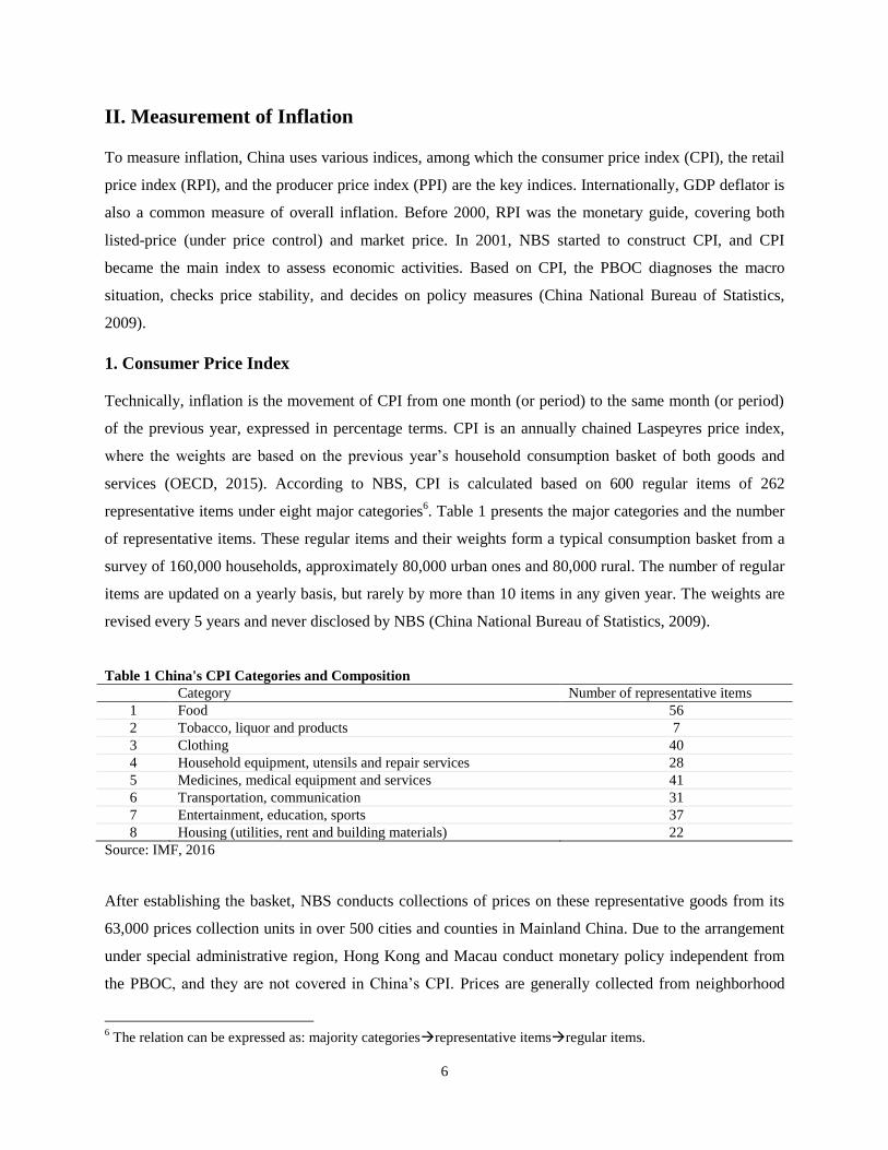
representative items under eight major categories6. Table 1 presents the major categories and the number

of representative items. These regular items and their weights form a typical consumption basket from a

survey of 160,000 households, approximately 80,000 urban ones and 80,000 rural. The number of regular

items are updated on a yearly basis, but rarely by more than 10 items in any given year. The weights are

revised every 5 years and never disclosed by NBS (China National Bureau of Statistics, 2009).

Table 1 China's CPI Categories and Composition

Category Number of representative items

1 Food 56

2 Tobacco, liquor and products 7

3 Clothing 40

4 Household equipment, utensils and repair services 28

5 Medicines, medical equipment and services 41

6 Transportation, communication 31

7 Entertainment, education, sports 37

8 Housing (utilities, rent and building materials) 22

Source: IMF, 2016. (IMF, 2016)

After establishing the basket, NBS conducts collections of prices on these representative goods from its

63,000 prices collection units in over 500 cities and counties in Mainland China. Due to the arrangement

under special administrative region, Hong Kong and Macau conduct monetary policy independent from

the PBOC, and they are not covered in China’s CPI. Prices are generally collected from neighborhood

6 The relation can be expressed as: majority categoriesrepresentative itemsregular items.

7

stores, large department stores, supermarkets of various sizes, shopping centers, and markets of various

kinds, and public service centers are also included (NBS cited in (Nakamura, et al., 2015)).

2. Retail Price Index

The RPI is the earliest price index in China, and it reflects the trend and extent of changes in retail prices

in both urban and rural areas in a certain time. RPI includes goods items only, covering 14 categories,

such as food, beverage and alcohol, garment and clothing, textile, medicine, cosmetics, newspapers and

magazines, machineries and electronics, etc.. Before 1994, agricultural production materials7 are under

RPI, and after 1994, it has been taken out to become a separate index. Collection of retail prices requires

huge amount of work, even though only 200 cities and 100 counties are surveyed for 400 goods sub-

categories. RPI is a weighted average index and functions as a benchmark to assess the purchasing power

of citizens and the market balances (MBAlib, 2014).

3. Producer Price Index

NBS uses PPI to measure the changes of ex-factory prices of all industrial goods, including both

production and consumption goods. It is also a Laspeyres index that records the price of first commercial

transaction of industrial products. By definition, PPI does not cover goods in agriculture sector and

services sector. PPI is constructed based on 40 percent of total industrial turnover nationwide surveying

over 60,000 enterprises. The weights of the product reflect the enterprise turnover, and are updated on an

interval of five years. The current PPI data comprise 41 industrial groups indicated in the Industrial

Classification for National Economic Activities (IMF, 2016).

4. GDP Deflator

The GDP deflator captures the price component in nominal GDP subtracting the quantity component

denoted by real GDP, hence it is also a measure of inflation. Given GDP covers all final goods and

services produced over a period, GDP deflator also has the broadest coverage of price level. GDP deflator

is usually obtained by dividing nominal over real GDP, hence it inherits measurement issues of GDP data.

There have been wide criticisms about unreliability of China’s GDP figure, not only from foreign

government and scholars (Rawski, 2001) (Koch-Weser, 2013), but also from domestic academics and

media (Meng & Wang, 2000) (Que & Zhong, 2005) (Xinhua News, 2014). Therefore, using the GDP

deflator to measure inflation in China is potentially problematic.

7 This includes fertilizer, pesticide, seeds, animals, machines, energy used for agriculture, etc..

8

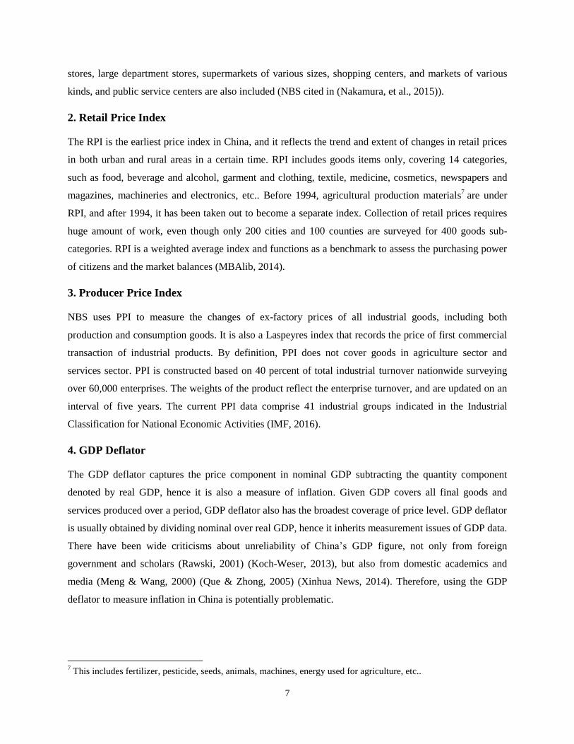
5. Comparison of Inflation Measures

Figure 1 plots inflation measured by different price level indices; it is clear that CPI and RPI inflation

move mostly in unity, and RPI inflation falls generally below CPI inflation. This might be because RPI

inflation only reflects the rise of good prices, not including services. PPI inflation differs from the CPI

and RPI, which may be due to data construction. The Inflation measured by GDP deflator in most times

diverges from CPI, which might be explained that it is a composition of CPI and other market price

indices (such as price index of investment goods, etc.).

In general, all the indices do not show huge divergence from each other, which confirms the price

transmission theory and the fact that their computations are inter-related8. In this paper, CPI and GDP

deflator inflation are used for econometric analysis.

Figure 1 Inflation in China in Different Measures

Source: CPI, RPI and PPI inflation are from China National Bureau of Statistics (2016), GDP deflator is from World

Bank World Development Indicators (2016). (China National Bureau of Statistics , 2016), (World Bank, 2016).

III. Policy Factors Related with Inflation in China

Besides measurement issues, given the unique economic development path, several policy factors have

direct influence on measurement of inflation in China, which are discussed in this sub-section.

8 For example, GDP deflator and CPI are linked by real GDP. To compile real GDP, countries generally use CPI and

other market price index to deflate nominal GDP, and GDP deflator adjusts the price effect of the nominal GDP.

Therefore, CPI is partially captured in GDP deflator.

%

9

1. Price Control

As a legacy of centrally-planned economy, China has a tradition of enforcing price regulation on

consumptions9, which ‘hides’ inflation to some degree. The price reform started in early 1980s to move

from the state control pricing system towards free market pricing system. From 1981 to 1994, a dual-track

pricing system was enforced on planned and surplus goods. The end of the dual-track pricing system saw

price liberalization, accompanied by inflation going through the roof (Yang, 2009).

The Price Law was introduced in 1998 to formally institutionalize price control, in response to the high

inflation created by market-determined prices in early 1990s. Even after WTO accession in 2001, price

control has been actively used to manage price level (Geiger, 2008). As CPI covers some goods and

services that are subject to price control, RPI might be a better measure of inflation than CPI (Mehrotra, et

al., 2007). In addition, Chinese government closely monitors and supervises the staple food market, which

has a large weight in both CPI and RPI, therefore, CPI and RPI inflation are potentially underestimated

through years (Mehrotra, et al., 2007). On the other hand, an OECD report in 2005 stated that by 2003,

over 96 percent of retail transactions were already according to market prices, which suggests a lessened

influence of price control on CPI and RPI (OECD, 2005).

2. Wage Control

Besides price control, wage control also has a close association with inflation in China. At the beginning

of China’s Reform and Open-Up policy in 1978, the wage rate is determined by central government.

Through years, there were several round of wage rate reforms, specifically in 1985, 1992 and 1994 (Yueh,

2004). In 1985, the Chinese government started to index wage rate to the price levels. This created a

feedback loop between inflation and wage rate – as higher inflation will lead to setting of a higher wage

rate, and higher wage rate in turn drives a higher inflation. This mechanism contributed to high inflations

in early 1990s, and forced the central government to conduct anther wage reform in 1994. The 1994

reform de-coupled wage rate and inflation, and linked wage to workers’ skill and productivity (Yueh,

2004).

3. Inflation Target

As mentioned in the introduction, the PBOC sets inflation targets since the Monetary Policy Reports 2002.

This target acts as a potential long-run target to enhance credibility of inflation management (Zhang &

9 Historically, there have been three types of prices in China: market-determined price, government guidance price,

and government price. Government guidance price is based on a benchmark or a range given by government, and

government price is fixed by government (Geiger, 2008).

10

Clovis, 2010), but in practice, China still follows a monetary target. In his speech at the seminar of the

2016 IMF Spring Meeting, Governor Zhou mentioned that ‘it is not yet realistic for China at this stage’ to

follow the single objective of inflation targeting (Zhou, 2016). Therefore, though China publishes

inflation target currently, its role remains symbolic.

IV. Evolution of Inflation in China

Following the policy factors that impact on inflation, it is necessary to look at the evolution of inflation in

China. From Figure 1, there seems to be significant fluctuations in inflation in China. Before 2000, China

experienced some high surges of inflation, especially in late 1980s and around 1994. Into the new century,

inflation seems quite tamed, seldom went beyond 5 percent. Whether there are structural breaks in the

evolution of inflation will be tested in econometric analysis, but in this section, the paper takes 1997/1998,

where China went from inflation to deflation, as the reference point10

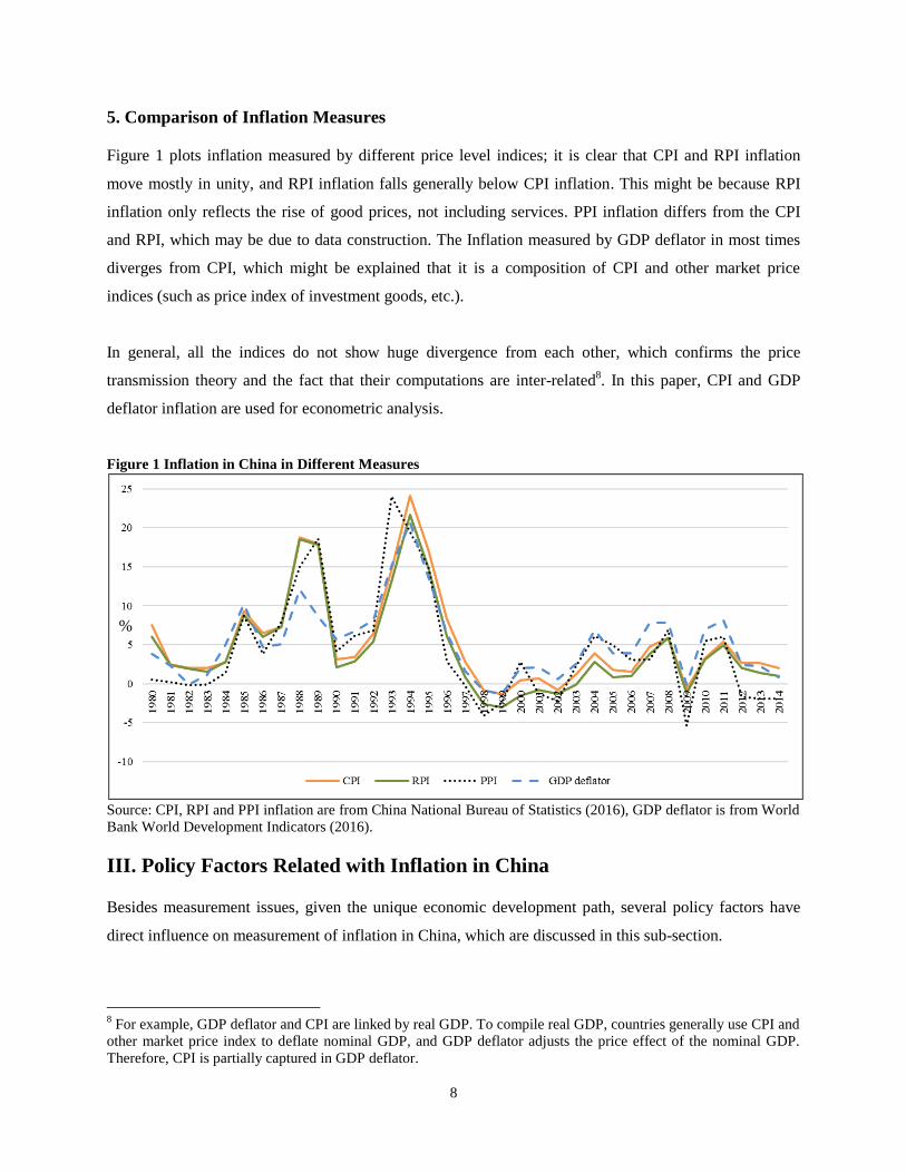
. The first period is of high inflation,

from 1981 to 1997, with average inflation registering close to 10 percent. The second period is marked

generally by deflation and low inflation, with average inflation registering below 2 percent.

Period 1: 1981 to 1997 (Figure 2)

Figure 2 Evolution of Inflation 1981-1997

Source: Author.

10

The separation of inflation evolution into two periods may seem arbitrary, however, this is for descriptive

evolution only. It is not associated with later econometric analysis.

11

The Chinese government started to liberalize the centrally administrated price in 1979 through the

‘Adjustment and Reform’ policy. Gradually, the agricultural price and industrial price began to rise, and

the momentum accelerated in 1985 when wages were indexed to price level, pushing inflation close to 10

percent per year. In the meantime, growth of money supply is accelerating, above 30 percent in 1985 and

1986. In December 1984, the PBOC was established to control the financial sector liquidity, through

minimum reserve requirements and credit quota system (Zhao, 2003).

The efforts to cool down the economy seemed to be effective in the earlier stage, but as prices got further

liberalized in 1987, inflation soared again, reaching almost 20 percent in 1988 and 1989 (Zhang & Clovis,

2010). The monetary tightening continued to 1989, and this affected the real economy of industrial

production, resulting in scarcity of good supply. So in the early 1990s, though inflation was brought under

control, China’s economic growth was hit hard, registering the lowest growth (below 5 percent) since the

1978 reform.

To prevent a hard landing of the economy, in 1990, the PBOC shifted its position from monetary

tightening to expansion. M2 grew by 29 percent in 1990 and nominal GDP went up by 9.3 percent in

1991. In 1992, further price liberalization allowed free market mechanism to determine prices, wages kept

on rising and credit control loosing, and economy started to show signs of overheating. In 1994, nominal

GDP grew by 13 percent, money supply by close to 50 percent, and inflation peaked at a historical height

of 24 percent. Besides money supply, other authors also identified demand shocks (Kojima, et al., 2005),

change in exchange rate policy (Xu, 2000) as factors that contributed to high inflation in 199411

. Hence,

Zhang and Clovis commented that in the first 10 years of the PBOC, its monetary policy was ‘inefficient

and unsuccessful in controlling inflation’ (2010).

Drastic measures were taken to contain inflation. The PBOC’s legal status was officially confirmed in

1995 (Zhang & Clovis, 2010), so it revised its policy goals to set inflation as a top priority (Fan, et al.,

2011), and decided to phase out the credit plan, which was one of its major tools (Zhao, 2003). Inflation

started to decelerate in 1995, and declined through to 1998. And then the Asian Financial Crisis occurred

when both economy and inflation decelerated in China. Drawing on the immediate past experience of

monetary stimulation, China mainly used fiscal ‘pump priming’ to support the economy and to avoid

large-scale unemployment during this crisis (Burdekin & Siklos, 2008).

11

Starting in 1994, China started to phase out the official exchange rate and pegged the RMB against the US dollar.

From 1980 to 1994, RMB has depreciated against the US dollar from 1 USD against less than 2 RMB to USD

against 8.2 RMB (Xu, 2000).

12

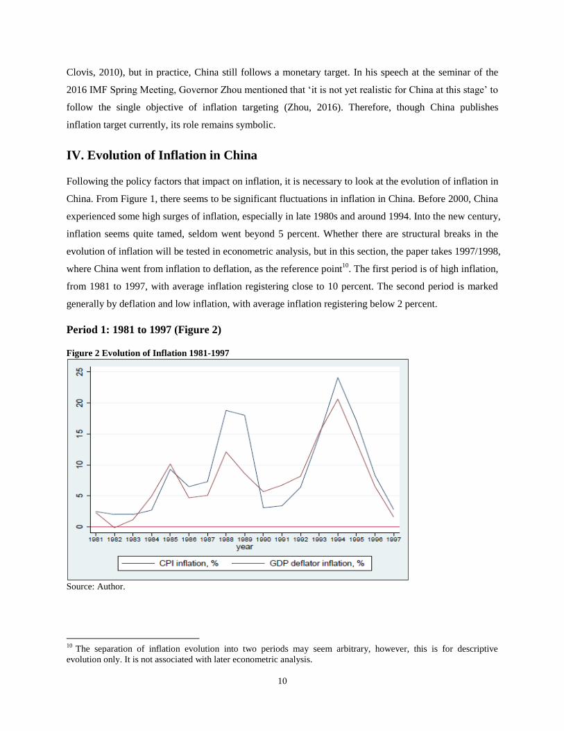
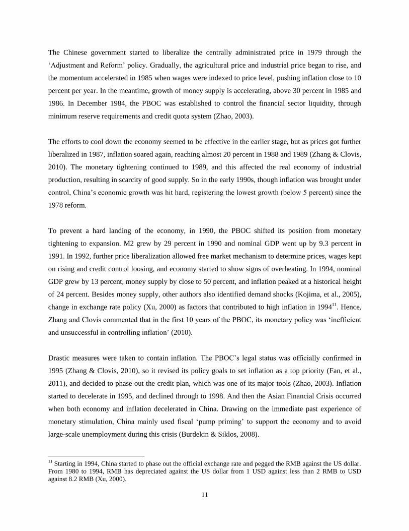
Period 2: 1998 to 2014 (Figure 3)

Figure 3 Evolution of Inflation 1998-2014

Source: Author.

The turn of the century in China was marked by relatively low and stable inflation. This has been noted

by Guerineau and Guillamont (2005), that China’s inflation of this period may be attributed primarily to

macroeconomic policy, as the movement of inflation closely tracked the shift of policy regime. In other

words, improvements in monetary policy weakened inflation substantially (Zhang, 2009). Towards the

end of 1990s, the PBOC adopted a composite strategy to conduct monetary policy with both quantity-

based and price-based tools, though quantity-based tools were still predominant, especially open market

operations and window guidance (Zhang & Clovis, 2010) (Pankki, 2015) (Gehringer, 2015).

In the second period of this study, inflation seems quite tamed, with only a couple of years registering

inflation rates above 5 percent. During this time, deflation became a big concern from 1998 to 2003.

Some scholars associated the deflation to productivity growth and appreciation of effective exchange rate

following the Asian Financial Crisis (Ha, et al., 2003); others argued that it was a structural issue of the

economy (Lin, 2004); the IMF linked it with lower commodity prices and WTO-related tariff cuts

(International Monetary Fund, 2003).

To address the deflation situation, the PBOC initiated an expansionary monetary cycle in 2003-04.

Money supply expanded by about 20 percent, but inflation was still mired in negative territory. In fact,

13

this might be explained by the lagged relationship between domestic loans and the inflation rate of around

5 to 12 months, identified by Geiger (2008). The inflation stayed at low levels in 2005 and 2006. The

PBOC adopted a mix of intensified window guidance, interest rate adjustment, and changes of reserve

requirement as its monetary policy tools. Economic growth steadily increased during this time, reaching

14 percent in 2007, and the symptom of overheating emerged. In light of this, the PBOC devised a

contractionary policy in November 2007, and further measures were taken in mid-2008 to restrain

monetary growth (Wong, 2011).

2008 is the year where the Global Financial Crisis stroke. As the crisis spread, the policy stance of PBOC

had a quick turn. The credit quota in the 2007 policy tightening was abolished, and the increase in money

supply exploded from 17 percent in 2008 to 30 percent in 2009, which is the so called ‘4 trillion RMB

stimulus program’. Though a temporary deflation took place in 2008, inflation immediately returned to

positive in 2009. Realizing there might be problems of over-dosage, in early 2010, PBOC again

deliberated on whether to tamp down growth momentum and slow credit expansion (Wong, 2011). The

real implementation took place in 2011, with money growth slowed down in a gradual and persistent

fashion; so did the inflation level.

14

Chapter 3: Major Theories on Inflation

‘Bad models lead to bad policy: central banks, for instance, focused on the small economic

inefficiencies arising from inflation, to the exclusion of the far, far greater inefficiencies arising

from dysfunctional financial markets and asset price bubbles’ (Stiglitz, 2010).

Various theories attempt to explain the causes of inflation, though most often these causes are intertwined.

It is important to identify the major causes, because different types of inflation are built on different

transmission mechanisms and require different policy responses. For example, demand-pull inflation

requires austerity policy to balance the economy, but austerity measures are generally in vain on cost-

push inflation (Holzman, 1960). This section focuses on three major theories on inflation: The Quantity

Theory of Money, the New Keynesian Phillips Curve, and the Structural Cost-push Theory. The first two

identify excessive demand as cause of inflation, hence are demand-pull; the latter one focuses on impact

of cost on aggregate supply, hence is cost-push. In reality, there is no way to clearly distinguish whether

an inflation phenomenon is demand-pull or cost-push. From theoretical point of view, demand-pull

inflation builds on the assumption of a natural or equilibrium state of the economy, while cost-push

inflation does not require such an assumption.

I. Quantity Theory of Money

‘One of the normal effects of an increase in the quantity of money is an exactly proportional

increase in the general level of prices’ (Fisher, 1911).

Among all theories that attempt to explain the causes of inflation, the Quantity Theory of Money enjoyed

its predominance since the turn of the 18th century. Its origin can trace back to Jean Bodin in mid-16th

century, and in 18th century David Hume established the causal relationship of money supply on price

(Humphrey, 1974). Later Milton Friedman integrated it with the general price theory and made it a

‘central and vigorous’ part of monetary analysis. Through the years, the Quantity Theory of Money was

introduced as one of the top ten economic principles, to put simply, ‘prices rise when the government

prints too much money’ (Mankiw, 2015).

The initial Quantity Theory of Money focused on only two variables, the money supply and inflation

(Fisher, 1912). But the popularity of the Quantity Theory of Money builds on its modern version, an

account of the relationship among money supply, inflation, and real economy. It asserts that the value of

money is determined by the quantity of money, and there are both short-run and long-run perspectives to

15

it. In the short run, change of money supply would affect real variables, such as output and employment,

which is termed ‘short-run effects’. In the long run, money is neutral, change of money supply would only

lead to changes in nominal variables, i.e. price level, and it is statistically unrelated to output growth. This

is captured by Friedman as ‘the neutrality of money’ (Friedman, 1970) (Lucas, 1972). The exact macro-

micro interaction of the short-run effects remains a controversy, but the long run relationship is well

established in the literature (McCandless & Weber, 1995) (Crowder, 1998) (Christensen, 2001) (De

Grauwe & Polan, 2005) (Rua, 2012)

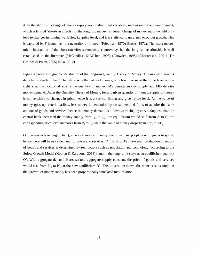
Figure 4 provides a graphic illustration of the long-run Quantity Theory of Money. The money market is

depicted in the left chart. The left axis is the value of money, which is inverse of the price level on the

right axis; the horizontal axis is the quantity of money. MS denotes money supply and MD denotes

money demand. Under the Quantity Theory of Money, for any given quantity of money, supply of money

is not sensitive to changes in price, hence it is a vertical line at any given price level. As the value of

money goes up, ceteris paribus, less money is demanded by consumers and firms to acquire the same

amount of goods and services; hence the money demand is a downward sloping curve. Suppose that the

central bank increased the money supply from Q1 to Q2, the equilibrium would shift from A to B, the

corresponding price level increases from P1 to P2 while the value of money drops from 1/P1 to 1/P2.

On the macro level (right chart), increased money quantity would increase people’s willingness to spend,

hence there will be more demand for goods and services (D’1 shift to D’2); however, production or supply

of goods and services is determined by real factors such as population and technology (according to the

Solow Growth Model (Koutun & Karabona, 2013)), and in the long run it stays at an equilibrium quantity

Q’. With aggregate demand increases and aggregate supply constant, the price of goods and services

would rise from P’1 to P’2 at the new equilibrium B’. This illustration shows the monetarist assumption

that growth of money supply has been proportionally translated into inflation.

16

Figure 4 The long-run Quantity Theory of Money

Source: Author.

The above figure also illustrates that in the long term, inflation is not related with the real variables, such

as output or income, real interest rate (Fisher Effect12

). This is in contract with the common view that

inflation erodes real income, so is the ‘Inflation Fallacy’.

1. The Empirical Model

The empirical model of the Quantity Theory of Money is built on the equation of exchange: PY = MV

(Fisher, 1911). In this equation, the left-hand side is the nominal GDP, which equals to the real GDP (Y)

times the general price level (P). The right-hand side denotes total spending, which equals to the money

supply (M) and the velocity of money (V). The velocity of money refers to the speed at which a typical

unit of currency is transacted from one person to another, or the speed of money changing hands

(Robinson, 1970).

Fisher, in 1911, amplified the original equation of exchange by separating the demand deposits from the

money supply. He proposed the equation: PY = MV + M’V’. In his equation, M is the amount of

currency or cash in circulation, V is the speed of circulation, M’ is the amount of demand deposits, and V’

is the circulation speed of demand deposits. He argued that the volume of demand deposits M’, though

holds a fixed relation to currency M, it has no direct impact on price level as currency M does. Therefore,

it is necessary to separate the demand deposits from currency (Fisher, 1911).

Fisher’s argument enjoyed limited popularity, because velocity is not directly observable, and to estimate

both velocity for cash and demand deposits is overly challenging if possible (Friedman & Schwartz,

12

The Fisher Effect refers to the phenomenon that an increase in inflation causes a proportional increase of the

nominal interest rate, while the real interest rate remains unchanged.

17

1982). In the interest of simplicity, most empirical model of the Quantity Theory of Money is a

transformation of the simple version of equation of exchange. Taking logarithm of the equation yields the

following linear equation:

(1) p + y = m + v or p = m – y + v

In the new equation, p denotes natural logarithm of the price level; y is real GDP logarithm; m is the

logarithm of money supply; and v is the logarithm in velocity of circulation. According to this equation,

inflation is related to the growth of money supply, economic performance and the circulation velocity. To

apply the equation, a key step is the estimation of velocity, as it plays an important role of mediating the

money supply and price levels.

Velocity

In the original equation of exchange, PY = MV, velocity can be understood as the ratio of total spending

to the money stock: nominal GDP/M. It indicates the number of transactions that happened on each unit

of money. With a high velocity, even a small money base can fund a large quantity of transactions. As

described in Figure 4, when the price is high, the value of money is low, if the central bank keeps the

money supply fixed, then velocity must rise to support the same level of economic activities.

Under the Quantity Theory of Money, the total physical output and the velocity of circulation are

assumed to be constant in the short run, and ‘independent of the quantity of money’ (Fisher, 1911).

Velocity is determined by economic and social relations, which are unaffected by the money stock

(Higgins, 1978); however, later Keynes challenged the view of quantity theorist and argued that velocity

is determined by the consumers’ spending habits and motives, risk aversion and expectations. This is also

called Liquidity Preferences Theory (Keynes, 1964).

Empirically, after the World War II, using V = PY / M to measure, the US velocity was far from constant.

In fact, it exhibited a persistent rising trend. It is explained that the increase of interest rate, the relatively

slower growth of money supply, and the growing availability of money substitutes have probably

contributed to the rise of velocity (Higgins, 1978).

Testable Model

If to follow the original Quantity Theory of Money, then velocity is treated as a constant; however,

empirically, most authors treat velocity as a function of nominal interest rate: v = 0 + 1r + e (Emerson,

2006) (Alimi, 2012). Here e is a random error. It is arguable how valid to use nominal interest rate as a

proxy of velocity. Figure 5 presents the relationship between velocity and lending interest rate. During the

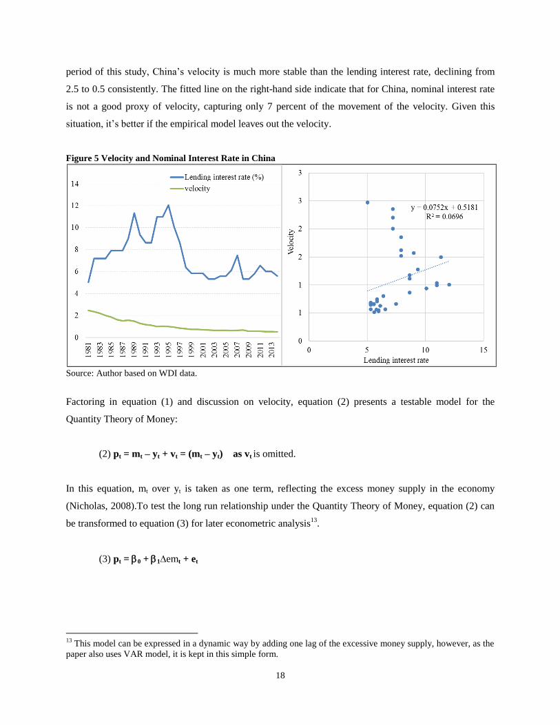
18

period of this study, China’s velocity is much more stable than the lending interest rate, declining from

2.5 to 0.5 consistently. The fitted line on the right-hand side indicate that for China, nominal interest rate

is not a good proxy of velocity, capturing only 7 percent of the movement of the velocity. Given this

situation, it’s better if the empirical model leaves out the velocity.

Figure 5 Velocity and Nominal Interest Rate in China

Source: Author based on WDI data.

Factoring in equation (1) and discussion on velocity, equation (2) presents a testable model for the

Quantity Theory of Money:

(2) pt = mt – yt + vt = (mt – yt) as vt is omitted.

In this equation, mt over yt is taken as one term, reflecting the excess money supply in the economy

(Nicholas, 2008).To test the long run relationship under the Quantity Theory of Money, equation (2) can

be transformed to equation (3) for later econometric analysis13

.

(3) pt = 0 + 1∆emt + et

13

This model can be expressed in a dynamic way by adding one lag of the excessive money supply, however, as the

paper also uses VAR model, it is kept in this simple form.

19

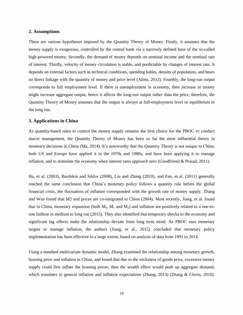
2. Assumptions

There are various hypotheses imposed by the Quantity Theory of Money. Firstly, it assumes that the

money supply is exogenous, controlled by the central bank via a narrowly defined base of the so-called

high-powered money. Secondly, the demand of money depends on nominal income and the nominal rate

of interest. Thirdly, velocity of money circulation is stable, and predictable by changes of interest rate. It

depends on external factors such as technical conditions, spending habits, density of population, and bears

no direct linkage with the quantity of money and price level (Alimi, 2012). Fourthly, the long-run output

corresponds to full employment level. If there is unemployment in economy, then increase in money

might increase aggregate output, hence it affects the long-run output rather than the price, therefore, the

Quantity Theory of Money assumes that the output is always at full-employment level or equilibrium in

the long run.

3. Applications in China

As quantity-based rules to control the money supply remains the first choice for the PBOC to conduct

macro management, the Quantity Theory of Money has been so far the most influential theory in

monetary decisions in China (Ma, 2014). It’s noteworthy that the Quantity Theory is not unique to China,

both US and Europe have applied it in the 1970s and 1980s, and have been applying it to manage

inflation, and to stimulate the economy when interest rates approach zero (Goodfriend & Prasad, 2011).

Ha, et al. (2003), Burdekin and Siklos (2008), Liu and Zhang (2010), and Fan, et al. (2011) generally

reached the same conclusion that China’s monetary policy follows a quantity rule before the global

financial crisis, the fluctuation of inflation corresponded with the growth rate of money supply. Zhang

and Wan found that M2 and prices are co-integrated in China (2004). Most recently, Jiang, et al. found

that in China, monetary expansion (both M0, M1 and M2) and inflation are positively related in a one-to-

one fashion in medium to long run (2015). They also identified that temporary shocks to the economy and

significant lag effects make the relationship deviate from long term trend. As PBOC uses monetary

targets to manage inflation, the authors (Jiang, et al., 2015) concluded that monetary policy

implementation has been effective to a large extent, based on analysis of data from 1991 to 2014.

Using a standard multivariate dynamic model, Zhang examined the relationship among monetary growth,

housing price and inflation in China, and found that due to the stickiness of goods price, excessive money

supply could first inflate the housing prices, then the wealth effect would push up aggregate demand,

which translates to general inflation and inflation expectations (Zhang, 2013) (Zhang & Clovis, 2010).

20

Studies on other economies also identified such an indirect transmission channel (Meltzer, 1995) (Adalid

& Detken, 2007).

However, not all research offers support to the Quantity Theory of Money in China. Wu found a negative

impact of money supply growth on inflation during 1993 to 2001 (2012). Sun and Ma (2004), Liu and

Chen (2012) found the relationship disappeared or weakened since 1998. Specifically, Sun and Ma used

surplus lag estimation recursively (Fixed Window Rolling Regression) to conduct a two-way Granger

causality test between money and price, and they found that money supply had become less effective to

stabilize the price level in deflation regime from 1998. Burdekin and Siklos explained that in the context

of deflation, China’s monetary policy is less effective, as purchase of non-essentials is postponed (2008).

This is especially true when China entered the World Trade Organization in 2001, with M2 expanded by

over 10 percent, wholesale prices dropped much more than consumer prices (Dai, 2002) (which suggests

that inflation in China is imported). The same view is strengthened by De Grauwe and Polan (2005),

based on a cross-country study of about 160 countries using cross-sectional estimation and panel data

approach, they found the relation between money growth and inflation held well in high- or hyper-

inflation countries; in low inflation countries (i.e. less than 10 percent yearly), there is no evidence for a

long-term Quantity Theory of Money.

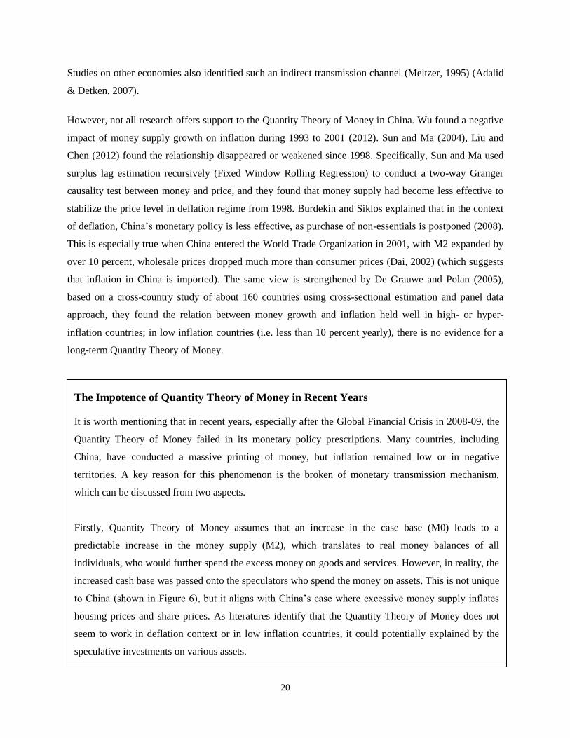
The Impotence of Quantity Theory of Money in Recent Years

It is worth mentioning that in recent years, especially after the Global Financial Crisis in 2008-09, the

Quantity Theory of Money failed in its monetary policy prescriptions. Many countries, including

China, have conducted a massive printing of money, but inflation remained low or in negative

territories. A key reason for this phenomenon is the broken of monetary transmission mechanism,

which can be discussed from two aspects.

Firstly, Quantity Theory of Money assumes that an increase in the case base (M0) leads to a

predictable increase in the money supply (M2), which translates to real money balances of all

individuals, who would further spend the excess money on goods and services. However, in reality, the

increased cash base was passed onto the speculators who spend the money on assets. This is not unique

to China (shown in Figure 6), but it aligns with China’s case where excessive money supply inflates

housing prices and share prices. As literatures identify that the Quantity Theory of Money does not

seem to work in deflation context or in low inflation countries, it could potentially explained by the

speculative investments on various assets.

21

II. New Keynesian Phillips Curve

The ‘dynamic relationship between inflation and unemployment remains a mystery’ (Mankiw,

2001).

The original Phillips Curve describes the negative relationship between wage inflation and the level of

unemployment in an economy (Phillips, 1958). The relationship is established based on an empirical

observation that unemployment and change in wage rates are inversely correlated in the United Kingdom

from 1986 to 1957. Under the condition that unemployment reflects the tightness of markets for all

factors of production (Okun’s Law)14

, Samuelson and Solow brought the relation to a broader level, being

14

According to the Okun’s Law, unemployment level is determined by economic output and aggregate demand

level (Okun, 1962).

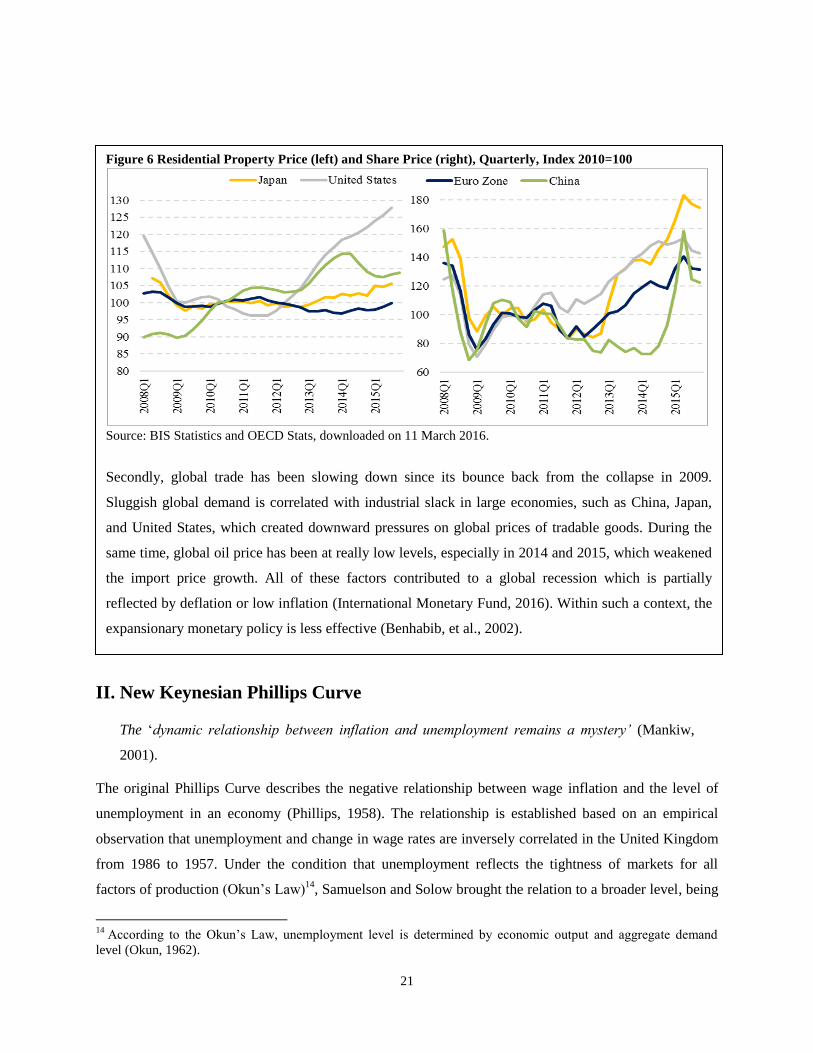
Figure 6 Residential Property Price (left) and Share Price (right), Quarterly, Index 2010=100

Source: BIS Statistics and OECD Stats, downloaded on 11 March 2016.

Secondly, global trade has been slowing down since its bounce back from the collapse in 2009.

Sluggish global demand is correlated with industrial slack in large economies, such as China, Japan,

and United States, which created downward pressures on global prices of tradable goods. During the

same time, global oil price has been at really low levels, especially in 2014 and 2015, which weakened

the import price growth. All of these factors contributed to a global recession which is partially

reflected by deflation or low inflation (International Monetary Fund, 2016). Within such a context, the

expansionary monetary policy is less effective (Benhabib, et al., 2002).

22

between unemployment and general price inflation (Samuelson & Solow, 1960). It is recognized that the

trade-off is non-linear – as inflation approaches zero, reducing it further would require larger increment in

unemployment.

In 1970s, Friedman observed that the trade-off between unemployment and wage rates was not stable.

Lower unemployment would lead to higher real wages, but higher real wages is not necessarily due to

lower unemployment, it might also be due to lower general price level. He introduced a new concept,

natural rate of unemployment, which corresponds to the real forces of the economy. When unemployment

is below the natural rate, inflation would accelerate; when unemployment is above the natural rate,

inflation would decline. Therefore, the natural rate of unemployment is also called Non-Accelerating

Inflation Rate of Unemployment (NAIRU) (Friedman, 1977), and the subsequent Phillips Curve is the

‘NAIRU Phillips Curve’ (Atkeson, 2001).

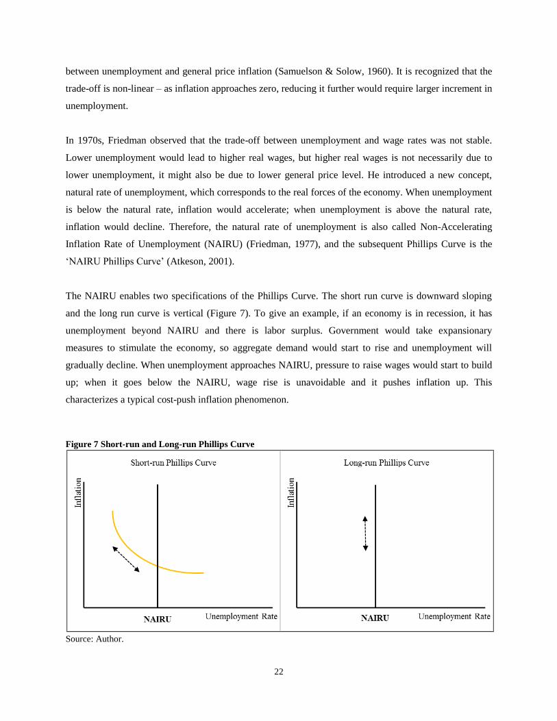
The NAIRU enables two specifications of the Phillips Curve. The short run curve is downward sloping

and the long run curve is vertical (Figure 7). To give an example, if an economy is in recession, it has

unemployment beyond NAIRU and there is labor surplus. Government would take expansionary

measures to stimulate the economy, so aggregate demand would start to rise and unemployment will

gradually decline. When unemployment approaches NAIRU, pressure to raise wages would start to build

up; when it goes below the NAIRU, wage rise is unavoidable and it pushes inflation up. This

characterizes a typical cost-push inflation phenomenon.

Figure 7 Short-run and Long-run Phillips Curve

Source: Author.

23

In addition, Friedman introduced the role of inflation expectation, which is formed on past inflation and

perfect information about the real economy. For example, if workers expect inflation to rise, they would

demand a higher wage. This leads to the ‘expectation-adjusted Phillips Curve’ (Friedman, 1977), also

called the New Keynesian Phillips Curve (Herz & Roeger, 2012) (Aidar, 2012). Under this situation,

inflation is forward looking and staggered nominal price setting plays a role in the process (Taylor, 1979)

(Calvo, 1983).

The New Keynesian Phillips Curve is widely used in monetary policy analysis (Fuhrer, 1995) (McCallum,

1997) (Blinder, 1997). In the short term, government could create unexpected inflation to temporarily

reduce unemployment. In the long term, unemployment stays at NAIRU, which is also the long-run

equilibrium of the real economy, so unemployment and inflation is not correlated. ‘Inflation is

everywhere a monetary phenomenon’, said Friedman, to refer to the ineffectiveness of monetary policy in

the long run.

1. The Empirical Model

As the Phillips Curve originates from empirics, initially it did not have a fixed specification. Only till the

curve is widely adopted in policy analysis, various tailored specifications start to emerge. As the long run

Phillips Curve is vertical, the empirical models mainly focused on the short term.

Basic model

A typical model of New Keynesian Phillips Curve looks like equation (4), with elements of both NAIRU

and inflation expectation incorporated (Staiger, et al., 1997) (Fabiani & Mestre, 2001) (Greenslade, et al.,

2003). The dependent variable is the difference between real inflation (t) and the expected inflation (et).

In Phillips’ study, this would be the difference between real wage and expected wage.

(4) ∆ t = t - et = (L) (t-1 -

et-1) + (L) (t-1 -

Nt-1) + t

The first term on the right-hand side is the difference between past real inflation (t-1) and expected past

inflation (et-1). The parameter (L) and (L) is the lag operator, which is consistent with findings of

many studies (Calvo, 1983) (Chen, 2008). This term captures the role of past inflation, can be viewed as

the inflation inertia. The model only adopts one lag, this is because as time goes by, the effect of lag

declines; also it is important to keep the model simple, as more variables would reduce the degrees of

freedom which further reduces the accuracy of the estimation.

24

The second term is the lag of the unemployment gap, between previous real unemployment (t-1) and

previous NAIRU (N

t-1). This term captures the impact of past change in employment on current inflation

difference. As unemployment gap is a close reflection of output gap, in some specifications, the

unemployment gap is replaced by output gap (Mehrotra, et al., 2007).

As discussed by Phillips (1958), the tradeoff between inflation and unemployment is not linear, but for

simplicity, the model adopts the linear form. The last term t is an idiosyncratic error, which is assumed to

follow a normal zero mean process with variance 2. It accounts for the potential supply shocks, such as

import prices or exchange rate fluctuation, that may shift the relationship. In this specification, there are

two elements that cannot be directly obtained from statistics, i.e. unobserved NAIRU and expected

inflation.

NAIRU

The empirical studies of the Phillips Curve usually treat NAIRU in two ways, either as a fixed value or as

a changing variable through years (Nickell, 1987) (Manning, 1994) (Llaudes, 2005). Using OLS

regression, Staiger, et al. (1997); Espinosa and Russell (1997); Ball and Mankiw (2002); Bernstein and

Baker (2013) calculated that US NAIRU has been historically around 6 percent. Based on data from 1987

to 2009, China’s NAIRU was estimated at 4.2 percent (Du & Lu, 2011). Using time series regression,

NAIRU is assumed to follow a random walk process or the Triangle Model15

(Gordon, 1997). Gordon

calculated that the US NAIRU fell from 6.2 percent to 5.6 percent from 1990 to 1996 (1997); Du and Lu

calculated that China’s NAIRU formed a concave downward curve from 1987 to 2008, peaking at 6.7

percent in 2005 and declined to 5.7 percent in 2008 (Du & Lu, 2009); Apergis et al. calculated the varying

NAIRU for Greece and found that from 1983 to 2000, it raised from 5 percent to 7.2 percent (2005).

Given these two approaches of NAIRU, results of various empirical studies are subject to questions. It is

hard to prove which approach is superior, hence depending on the approach, the result would be different.

Operationally, a common methodology to derive NAIRU is statistical filtering, i.e. Hodrick-Prescott (HP)

filter, Kalman filter, and so on. These filters try to identify a NAIRU around which unemployment

fluctuates. However, filters are purely statistically treatment, and do not factors in other macro factors and

are sensitive to smoothing parameters that are forced on the series (Fabiani & Mestre, 2000) (Benes &

N'Diaye, 2004).

15

According to the Triangle Model, inflation is driven by demand-pull, cost-push, and inflation inertia factors,

expressed in equation t = ∑ 𝐾𝑡=1 t-k + Xt + Yt +t

25

Expected Inflation

In the New Keynesian Phillips Curve, the expected inflation could be used as a policy tool if the central

bank can influence people’s expectation (Cogley & Sbordone, 2008). Same as NAIRU, expected inflation

is not directly available from data, and needs to be derived from calculations. There are two schools of

thought on expected inflation: backward-looking or adaptive inflation is formed based on past inflation;

and forward-looking inflation uses inflation forecasts that are observable in real time (Brissimis &

Magginas, 2008). Most literatures specify it as a random walk process (Fuhrer, 1995) (Espinosa &

Russell, 1997) (Staiger, et al., 1997) (Xiao & Chen, 2004), as in equation (5):

(5) et = t-1 + et

This means the expected inflation is based on the past period inflation as short-term forecast and in the

long run, inflation always equals to the expected inflation. In the equation, et, as a white noise error, is

independently and identically distributed. It is assumed to be uncorrelated with t at all leads and lags,

therefore equation (4) t - et = ∆t is the same as t - t-1 = ∆t.

Augmented Model

In many cases, the New Keynesian Phillips Curve also includes other macro variables, denoted as Xt. to

capture potential shocks to the economy. This forms the augmented model:

(6) t - et = (L) (t-1 -

et-1) + (L) (t-1 -

Nt-1) + (L) Xt + t

In the equation, Xt would absorb supply shocks that was initially captured by the error term, reducing the

chances of omitted variable bias and strengthening the stability of the model. Usually Xt includes oil price

and import price index, and factors such as raw material price, food price, interest rate, money supply, and

investment could also be included (Melihovs & Zasova, 2014) (Du & Lu, 2011).

2. Assumptions

The New Keynesian Phillips Curve is built on a few assumptions. Firstly, it is assumed that workers can

demand a wage level that is based on expected changes in the price level or cost of living (Fuhrer, 1995).

In reality, there might be labor market rigidity, unionization, multi-year nominal contracts, and social

norms against wage change (Llaudes, 2005), therefore, workers’ wage cannot follow the general price

level. Secondly, the New Keynesian Phillips Curve assumes that people can form rational expectation

based on all available information. Though this aligns with the rational expectation assumption in

26

economics (Lucas, 1972), it is hard to prove it in practice. In equation (2), expectation is a random

process on past inflation, in a way, it ignores the influence of current unemployment and monetary policy,

which may have shifted the relationship among macro indicators, as says the famous Lucas Critique.

Thirdly, though playing a key role in New Keynesian Phillips Curve, NAIRU remains an ideological term.

It assumes that labor market is competitive and reaches a unique equilibrium at the natural rate, which

ignores the labor market rigidity in practice16

.

3. Application to China

In recent years, many studies attempted to investigate a New Keynesian Phillips Curve for China.

Focusing on theories, some scholars looked at the assumptions, constructions and transformation of the

Phillips Curve and constructed tailored Phillips Curve for Chinese economy. Focusing on data, some

scholars concentrated on the fitness of the model and found that the New Keynesian Phillips Curve

explains data better than the traditional Phillips Curve.

Though Shi, et al. (2004), Liu and Zhang (2001) identified a stable relationship between output gap and

inflation during 1980-2001, many studies conclude that the New Keynesian Phillips Curve does a better

job. Ha, et al (2003), using data from 1989 to 2002, found that New Keynesian Phillips Curve accounted

for inflation dynamics in China better than the traditional Phillips Curve. Same findings are reached by

Gerlach and Peng, they estimated the output gap for 1982-2003, and found that the standard Phillips

Curve does not fit the data well. But after controlling the autoregressive process and including policy

factors, such as price deregulation, trade liberalization, and exchange rate reform, the model explains

inflation in China well (Gerlach & Peng, 2006). Zhao and Yong noted that inflation expectation plays a

role in driving inflation (2004). Using unemployment gap in urban areas, Zhang found a vertical Phillips

Curve for China from 1979 to 2000, that means inflation policy did not have any impact on

unemployment rate (Zhang, 2003).

Funke noted the large explanatory power of lead and lag inflation on current inflation, but the significance

of output gap or marginal cost is fragile (2006). Kojima, et al. used electricity consumption per unit of

capital as the proxy of output gap, and found that wage growth, raw material price, and the money gap are

important factors of inflation (2005).

16

This is interpreted as unemployed persons are assumed to choose to be unemployed.

27

III. Structural Cost-push Theory

‘The money supply in a credit-money economy is endogenous, not exogenous – it varies in direct

response to changes in the public demand to hold cash and bank deposit and not independently of

that demand’ (Kaldor, 1986, p. 47)

Analyzing inflation from a cost-push perspective started in 1800s, though at that time it was not yet

formalized as a theory on inflation (Humphrey, 1976). The technique was revived in the late 1950s

against the background of tight monetary condition, government surplus, rising unemployment, and

creeping inflation in the United States, and since then, the Structural Cost-push Theory on inflation

developed.

The Structural Cost-push Theory bears close linkage with the Post-Keynesian Theory of Inflation. The

Post-Keynesian Theory posits an endogenous money supply and profit-driven pricing rule by firms

(Smithin, 2003). The Structuralist Theory extends the Post-Keynesian Theory, and analyzes relative

prices among different sectors. Due to structural transformation of the economy, certain sectors

experience price rises relative to other sectors, and this rise of relative prices is passed on to the broad

economy and leads to an overall inflation. Therefore, the cost-push inflation directly affects the supply-

side of the economy and precedes any changes in aggregate demand (Javed & Akram, 2010).

The Structural Cost-push Theory emphasizes the fact that structural differences / shocks change the

relative prices of production factors, and increase the cost of production in certain sectors; to keep the

profit level, the firms revise up the prices and this is passed onto consumers in the form of higher prices.

Consumers are at the same time labor to the all firms, so they would demand higher wages to keep their

real income level, which further pushes up prices (Majumder, 2006). This forms an inflation spiral. The

structural causes can be sectoral differences arisen from market power (such as oligopoly and monopoly)

(Makochekanwa, 2007), productivity growth, bargaining power of trade unions (Javed & Akram, 2010),

supply shocks (Mankiw, 1997), and import content in production (Harvey, 1991), etc.

Typically, there are three main channels that transfer the cost of production to a rising price level: wage

push, profit push and material-cost push (Humphrey, 1998). These channels tend to reinforce each other

in reality (Jongwanich & Park, 2008). Among the three channels, wage is a key determinant of the firms’

pricing behavior. In aggregate, it accounts for about two-thirds of total cost. When wage rise exceeds the

productivity gain, it exerts upward pressure on prices; or nominal wage adjusts to higher inflationary

28

expectations, wage pushes inflation. Therefore, wages are not strictly endogenous or exogenous, as it is

determined by the bargaining power of labor, as well as inflation expectation (Friedman, 1968) (Perry &

Cline, 2013).

The second cost-push channel is profit. As Cost-push Theory does not require the competitive market

condition, firms typically price with a mark-up factor on top of their production cost. This pricing rule is

practiced by oligopolistic or monopolistic firms under the classic theories, and mark-up affects the

profitability of the firms. A higher mark-up means a higher price for consumers, following the logic of

inflation spiral, price rises would spread to other sectors, and the general price level would also rise,

hence this is profit-push inflation.

The last cost-push channel is material cost. Materials, as input, affect many stages of production.

Materials can be sourced from both domestic and foreign markets, hence both domestic and foreign

supply shocks impact on their prices. In addition, foreign sourced materials also expose domestic

economy to exchange rate risk (Harvey, 1991). Some key materials that are vital in inflation process are

agricultural produces, energy such as oil and gas, and minerals and chemicals.

Figure 8 presents a graphical view of the Structural Cost-push Theory. Either from one of the three

channels or their combinations, the cost of production rises and the aggregate supply curve shifts upward.

As the aggregate supply decreases, transactions are also reduced, resulting in a higher price P2 and a

lower quantity Q2. This is also characterized as the phenomenon of stagflation, and is one of the

difference between demand-pull and cost-push inflation - demand-pull inflation is usually accompanied

by unemployment fall, while cost-push inflation is accompanied by unemployment rise (Holzman cited in

(Fan, 2010)).

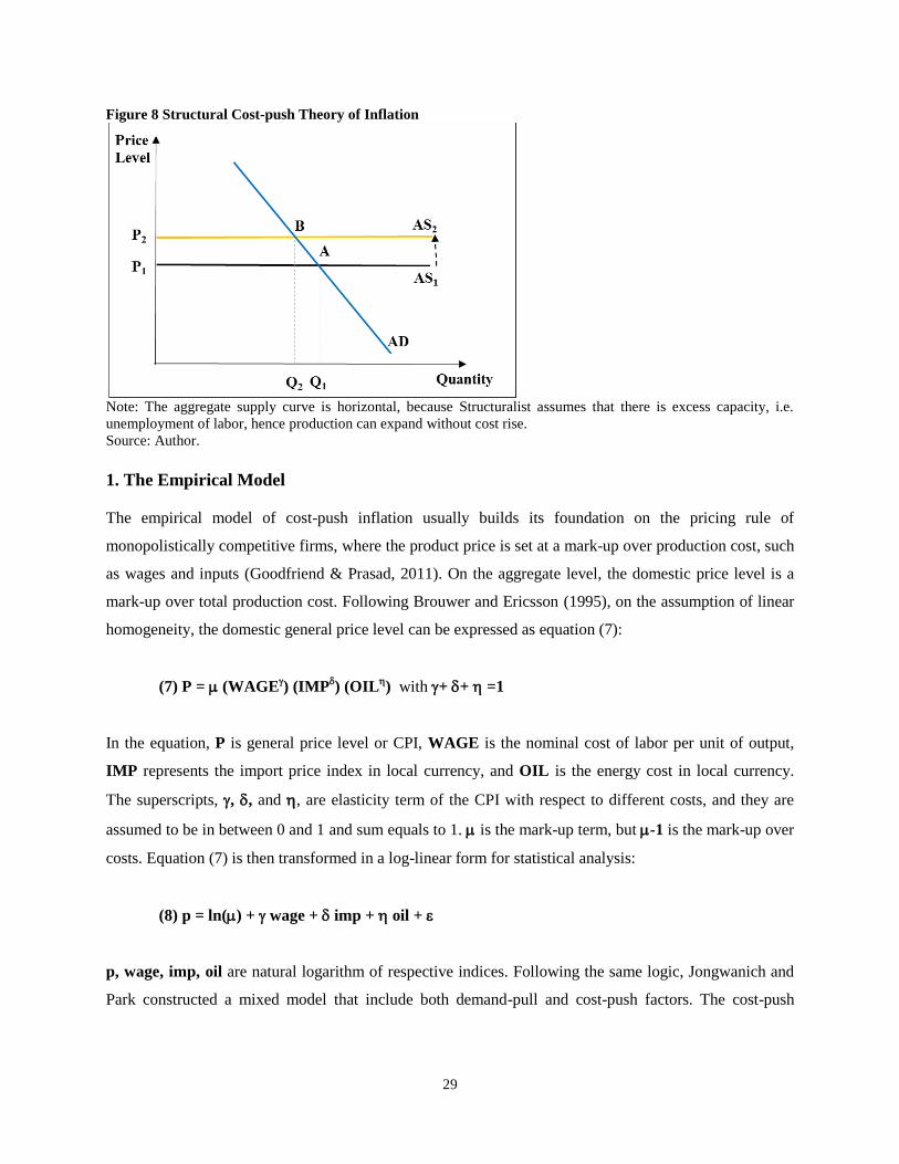
29

Figure 8 Structural Cost-push Theory of Inflation

Note: The aggregate supply curve is horizontal, because Structuralist assumes that there is excess capacity, i.e.

unemployment of labor, hence production can expand without cost rise.

Source: Author.

1. The Empirical Model

The empirical model of cost-push inflation usually builds its foundation on the pricing rule of

monopolistically competitive firms, where the product price is set at a mark-up over production cost, such

as wages and inputs (Goodfriend & Prasad, 2011). On the aggregate level, the domestic price level is a

mark-up over total production cost. Following Brouwer and Ericsson (1995), on the assumption of linear

homogeneity, the domestic general price level can be expressed as equation (7):

(7) P = (WAGE) (IMP

) (OIL

) with + + =1

In the equation, P is general price level or CPI, WAGE is the nominal cost of labor per unit of output,

IMP represents the import price index in local currency, and OIL is the energy cost in local currency.

The superscripts, , , and , are elasticity term of the CPI with respect to different costs, and they are

assumed to be in between 0 and 1 and sum equals to 1. is the mark-up term, but -1 is the mark-up over

costs. Equation (7) is then transformed in a log-linear form for statistical analysis:

(8) p = ln() + wage + imp + oil +

p, wage, imp, oil are natural logarithm of respective indices. Following the same logic, Jongwanich and

Park constructed a mixed model that include both demand-pull and cost-push factors. The cost-push

30

element, shown below, extends to food prices (food), as food accounts for a substantial portion in CPI

basket (Jongwanich & Park, 2008).

(9) pt = 0 + 1oilt + 2 foodt + 3 impt + et

From the perspective of the three cost-push channels discussed above, none of these models cover the

cost-push elements comprehensively, hence it’s necessary to combine models to construct a more holistic

model (10) for the later econometric analysis.

(10) pt = 0 + 1waget + 2 profitt + 3 foodt + 4 oilt + 5 impt + et

with 0 + 1 + 2 + 3 + 4 + 5 = 1

2. Assumptions

A few key assumptions support the Structural Cost-push Theory. Firstly, markets are not necessarily

competitive and firms enjoy certain discretion to set prices; firms would pass the increase in cost of

production to consumers (Hansen, 1951). Secondly, aggregate demand is not price elastic in the short run,

so the upward push in costs is autonomous of the demand conditions (Fan, 2010). Thirdly, the sector

experiencing a relative price rise is an important sector in the economy and the inputs, either domestic or

imported, are crucial in production, hence the price of this sector affects the cost structure of firms in the

whole economy. Fourthly, specific to wage-push inflation, it is necessary that trade union or

institutionalized labor enjoy substantial control on the labor supply, so that they can bargain for wage

changes (Addison & Burton, 1980) (Perry & Cline, 2013). In other words, nominal wage rigidity does not

affect inflation dynamics (Peneva & Rudd, 2015). Lastly, the cost-push theory assumes that money is

endogenous, as in Post-Keynesian Theory.

3. Application in China

Comparing with the Quantity Theory of Money and New Keynesian Phillips Curve, there is significantly

less research dedicated to cost-push inflation in China. Zhang studied inflation in China from 2000

onwards, and found that demand-pull factors play a more important role than cost-push factors in

determining inflation. But she predicted that as Chinese economy transforms towards a more market-

oriented system, cost-push factors may become significant (Zhang, 2012). Zuo focused on inflation before

and during global financial crisis in 2008, and she concluded that before 2007, aggregate demand is the

main cause of inflation in China and since the global financial crisis, cost-push factors kicked in and

31

became more accountable for inflation (Zuo, 2008). However, Zuo’s conclusion is questionable, as she

did not use any data or model to support her argument.

Quite a number of research found that both demand-pull and cost-push factors affect inflation in China

(Chen, 2008) (Jongwanich & Park, 2008) (Fu, et al., 2011). Su in 2011 published an article claiming that

demand and supply factors influence inflation equally in China, and advocated a policy to expand

aggregate supply and reduce aggregate demand (Su, 2011).

Comparing excess money supply (as a proxy of demand-pull factors) and excess wage rise from 1985 to

2007, Fan identified that China’s inflation is more related to monetary factors rather than cost factors

(2008)17

. Similarly, Fu, et al. found cost-push factors have less impact on inflation in China than excess

money supply and excess demand (2011).

On other factors, Lu and Hou used the structural vector auto-regressive model on cost-push inflation, and

identified that the international food price is associated with general price level in China (Lu & Hou,

2013); while Zhang’s research confirmed that China’s inflation behavior is mainly affected by imported

inflation (Zhang, 2013).

IV. Summary

As a summary, the three major theories differ significantly in how they view the inflation, how the

theoretical modes are built, assumptions and results. Especially the Structural Cost-push Theory does not

involve movement of aggregate demand curve and does not assume competitive markets and equilibrium

economy as the other two theories. In addition, the Structural Cost-push Theory differs fundamentally in

conducting the monetary policy. The Quantity Theory of Money defines money supply to be exogenously

controlled by the central bank, hence excess money supply proceeds price changes and results in inflation.

The New Keynesian Phillips Curve specifies that excessively rapid growth of the economy or fiscal

imbalances lead to excess demand, which drives up inflation, hence money stock changes are viewed

endogenous. Under the cost-push theory, money supply is endogenous to the economy and money growth

accommodates the price changes, hence price change proceeds money growth and money growth sustains

inflation (Batten, 1981) (DeLong, 1996) (Humphrey, 1998) (Smithin, 2003) (Mishkin, 2007).

17

The author used VAR model and impulse response function to identify the relationship among import price level,

excess wage, money supply and inflation

32

Chapter 4: Econometric Analysis

As shown in the empirical model of each theory, the main variable of interest is inflation, and explanatory

variables differ from theory to theory. Data of some variables can be directly obtained from national and

international databases, the rest need some calculation and construction to reach. The paper uses data

from both China’s National Statistics Bureau (2016) and international databases, namely the World Bank

World Development Indicators (2016), the International Monetary Fund (IMF) International Finance

Statistics (2016), and databases of the Food and Agriculture Organization (2016), International Labor

Organization (2016), and the World Trade Organization (2016). Though it is preferable to obtain all the

variable from the same source, given the variables involved and as well as time span of the data, only by

drawing from all of these databases, the paper can pool together a feasible dataset. As the model are

clearly defined, most variables use the data that corresponds to their meaning, however, for Structuralist

model, data availability is limited, so in certain cases, proxies are used.

I. Summary of Variables

The dataset includes a maximum of 34 years of annual data, wherever possible, from 1981 to 201418

.

Table 2 (on next page) presents a full list of variables in the analysis. Inflation is both measured by CPI

and GDP deflator. For econometric investigation, CPI inflation is used for primary analysis and GDP

deflator is used as robustness check. From 1981 to 2014, China experienced both high inflation and

deflation. The peak of CPI inflation occurred in 1994 at 24.1 percent and deflation occurred in four years,

namely 1998, 1999, 2002 and 2009, where 1999 registered the highest deflation of 1.4 percent. If

measured by GDP deflator, inflation peaked also in 1994, while deflation set in in 1982, 1998/99, and

2009.

18

Ideally, study of inflation should use quarterly or monthly data, however, due to majority of variables only have

annual data available from open public sources, this paper opts for analysis of annual data. This is one of the

weaknesses of the study.

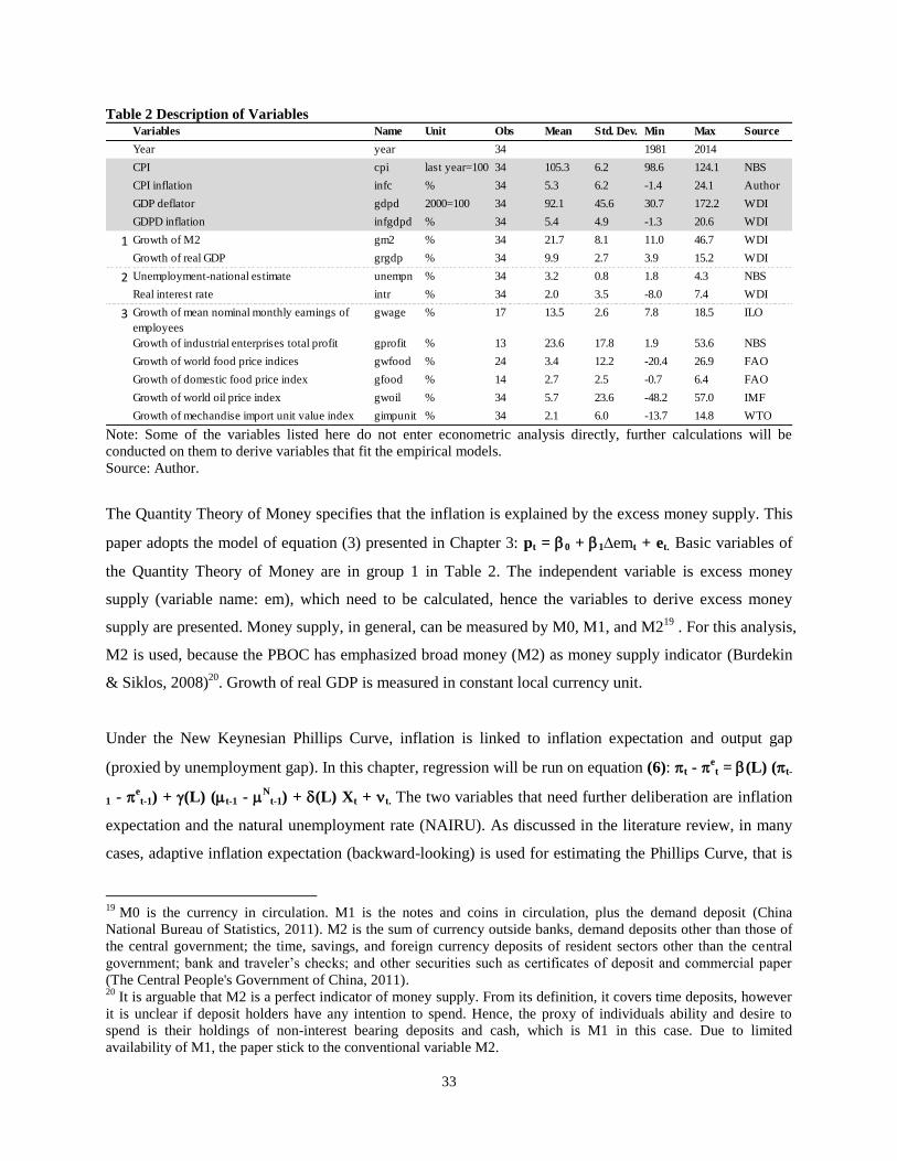
33

Table 2 Description of Variables

Note: Some of the variables listed here do not enter econometric analysis directly, further calculations will be

conducted on them to derive variables that fit the empirical models.

Source: Author.

The Quantity Theory of Money specifies that the inflation is explained by the excess money supply. This

paper adopts the model of equation (3) presented in Chapter 3: pt = 0 + 1∆emt + et. Basic variables of

the Quantity Theory of Money are in group 1 in Table 2. The independent variable is excess money

supply (variable name: em), which need to be calculated, hence the variables to derive excess money

supply are presented. Money supply, in general, can be measured by M0, M1, and M219

. For this analysis,

M2 is used, because the PBOC has emphasized broad money (M2) as money supply indicator (Burdekin

& Siklos, 2008)20

. Growth of real GDP is measured in constant local currency unit.

Under the New Keynesian Phillips Curve, inflation is linked to inflation expectation and output gap

(proxied by unemployment gap). In this chapter, regression will be run on equation (6): t - et = (L) (t-

1 - et-1) + (L) (t-1 -

Nt-1) + (L) Xt + t. The two variables that need further deliberation are inflation

expectation and the natural unemployment rate (NAIRU). As discussed in the literature review, in many

cases, adaptive inflation expectation (backward-looking) is used for estimating the Phillips Curve, that is

19

M0 is the currency in circulation. M1 is the notes and coins in circulation, plus the demand deposit (China

National Bureau of Statistics, 2011). M2 is the sum of currency outside banks, demand deposits other than those of

the central government; the time, savings, and foreign currency deposits of resident sectors other than the central

government; bank and traveler’s checks; and other securities such as certificates of deposit and commercial paper

(The Central People's Government of China, 2011). 20

It is arguable that M2 is a perfect indicator of money supply. From its definition, it covers time deposits, however

it is unclear if deposit holders have any intention to spend. Hence, the proxy of individuals ability and desire to

spend is their holdings of non-interest bearing deposits and cash, which is M1 in this case. Due to limited

availability of M1, the paper stick to the conventional variable M2.

Variables Name Unit Obs Mean Std. Dev. Min Max Source

Year year 34 1981 2014

CPI cpi last year=100 34 105.3 6.2 98.6 124.1 NBS

CPI inflation infc % 34 5.3 6.2 -1.4 24.1 Author

GDP deflator gdpd 2000=100 34 92.1 45.6 30.7 172.2 WDI

GDPD inflation infgdpd % 34 5.4 4.9 -1.3 20.6 WDI

1 Growth of M2 gm2 % 34 21.7 8.1 11.0 46.7 WDI

Growth of real GDP grgdp % 34 9.9 2.7 3.9 15.2 WDI

2 Unemployment-national estimate unempn % 34 3.2 0.8 1.8 4.3 NBS

Real interest rate intr % 34 2.0 3.5 -8.0 7.4 WDI

3 Growth of mean nominal monthly earnings of

employees

gwage % 17 13.5 2.6 7.8 18.5 ILO

Growth of industrial enterprises total profit gprofit % 13 23.6 17.8 1.9 53.6 NBS

Growth of world food price indices gwfood % 24 3.4 12.2 -20.4 26.9 FAO

Growth of domestic food price index gfood % 14 2.7 2.5 -0.7 6.4 FAO

Growth of world oil price index gwoil % 34 5.7 23.6 -48.2 57.0 IMF

Growth of mechandise import unit value index gimpunit % 34 2.1 6.0 -13.7 14.8 WTO

34

a random walk process based on the past inflation (Gali & Gertler, 1999). Based on this, the difference

between inflation and its expectation is just the inflation difference (variable name: infcgap or

infgdpdgap). NAIRU is assumed to be 4.2% (calculated by other author, please refer to Chapter 3) in this

paper, and not calculated separately. This is because it is quite difficult to estimate NAIRU, especially

when the economy is undergoing significant transformation (Ha, et al., 2003). Another regressor in this

equation, unemployment gap (variable name: unempgap) is measured by unemployment rate, estimated

by NBS, minus the NAIRU. To capture the general monetary policy context, real interest rate is also a

variable for New Keynesian Phillips Curve.

The Structuralist Cost-push Theory links inflation with various inputs cost levels, such as wages, profit

level, energy price, import price, etc. The main equation used in this section is equation (10): pt = 0 +

1waget + 2 profitt + 3 foodt + 4 oilt + 5 impt + et. One constraint on analyzing inflation in China

from cost-push angle is that there is very few data available for certain indicators. For example, there are

only 13 years of data for profit level, 14 years of data for domestic food price level, and 17 years of data

for wage level. Regarding the sources, Growth of mean nominal monthly earnings of employees are

estimated by ILO, reflecting the changes to wage level through years. Profit level is captured by the

industrial enterprises total profit21

. Industrial enterprises are only part of the economy; as agriculture and

services are not included, this indicator may be biased. Food price is measured at two levels, the world

level and domestic level. In theory, it makes more sense to use domestic food price index for Cost-push

Theory, because of the price control on food in China. Oil price level is a world index, which is a variable

with the largest fluctuation in the dataset22

. Lastly, the import price is measured by merchandise import

unit value index, which is a deflator of imports by China. It is noteworthy that not every variable has data

for all years. Especially for the cost-push theory, analysis is severely constrained by data availability.

II. Stationarity of Variables

Besides evolution, another important character of these variables is their stationarity, which determines

the form of data that enters the econometric analysis in the next chapter. Using Augmented Dickey-Fuller

Test, explanatory variables are tested on their stationarity and properties that make the series stationary in

21

Though from the pricing rule, profit level is an explanatory variable, in certain discussions of Post-Keynesians,

when profit share falls, there is a greater pressure for inflation. Given the difficulties in obtaining profit data, profit

level data is already quite patchy, the paper will not try to get general revenue figures to derive profit share. Even

there are data of revenue, there is an issue of compatibility with profit level data. 22

The world oil price index has limited relevance to the domestic price of oil, as oil is one of the product under price

control.

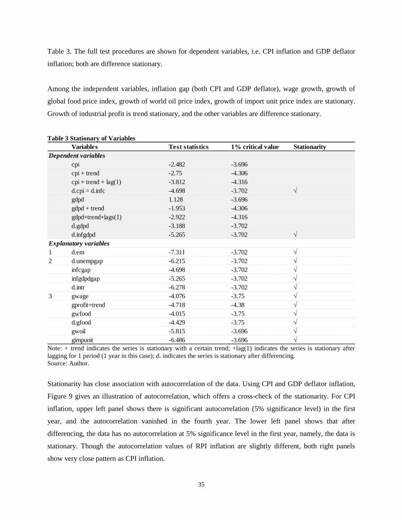
35

Table 3. The full test procedures are shown for dependent variables, i.e. CPI inflation and GDP deflator

inflation; both are difference stationary.

Among the independent variables, inflation gap (both CPI and GDP deflator), wage growth, growth of

global food price index, growth of world oil price index, growth of import unit price index are stationary.

Growth of industrial profit is trend stationary, and the other variables are difference stationary.

Table 3 Stationary of Variables

Note: + trend indicates the series is stationary with a certain trend; +lag(1) indicates the series is stationary after

lagging for 1 period (1 year in this case); d. indicates the series is stationary after differencing.

Source: Author.

Stationarity has close association with autocorrelation of the data. Using CPI and GDP deflator inflation,

Figure 9 gives an illustration of autocorrelation, which offers a cross-check of the stationarity. For CPI

inflation, upper left panel shows there is significant autocorrelation (5% significance level) in the first

year, and the autocorrelation vanished in the fourth year. The lower left panel shows that after

differencing, the data has no autocorrelation at 5% significance level in the first year, namely, the data is

stationary. Though the autocorrelation values of RPI inflation are slightly different, both right panels

show very close pattern as CPI inflation.

Variables Test statistics 1% critical value Stationarity

cpi -2.482 -3.696

cpi + trend -2.75 -4.306

cpi + trend + lag(1) -3.812 -4.316

d.cpi = d.infc -4.698 -3.702

gdpd 1.128 -3.696

gdpd + trend -1.953 -4.306

gdpd+trend+lags(1) -2.922 -4.316

d.gdpd -3.188 -3.702

d.infgdpd -5.265 -3.702

1 d.em -7.311 -3.702

2 d.unempgap -6.215 -3.702

infcgap -4.698 -3.702

infgdpdgap -5.265 -3.702

d.intr -6.278 -3.702

3 gwage -4.076 -3.75

gprofit+trend -4.718 -4.38

gwfood -4.015 -3.75

d.gfood -4.429 -3.75

gwoil -5.815 -3.696

gimpunit -6.486 -3.696

Dependent variables

Explanatory variables 

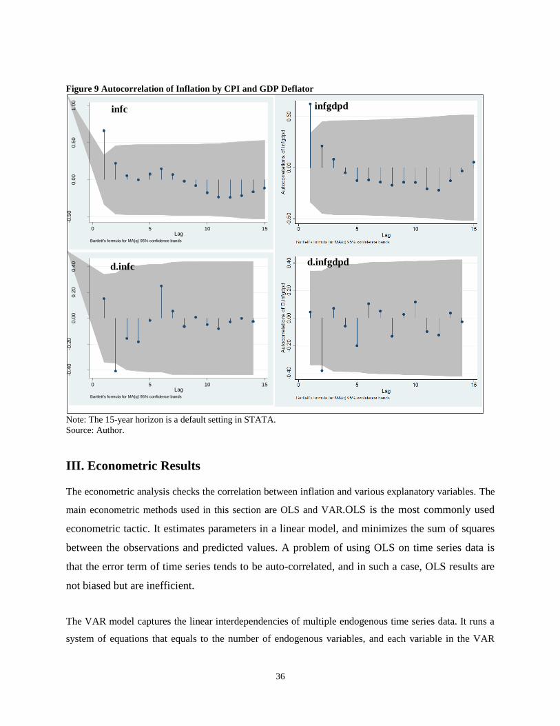
36

Figure 9 Autocorrelation of Inflation by CPI and GDP Deflator

Note: The 15-year horizon is a default setting in STATA.

Source: Author.

III. Econometric Results

The econometric analysis checks the correlation between inflation and various explanatory variables. The

main econometric methods used in this section are OLS and VAR.OLS is the most commonly used

econometric tactic. It estimates parameters in a linear model, and minimizes the sum of squares

between the observations and predicted values. A problem of using OLS on time series data is

that the error term of time series tends to be auto-correlated, and in such a case, OLS results are

not biased but are inefficient.

The VAR model captures the linear interdependencies of multiple endogenous time series data. It runs a

system of equations that equals to the number of endogenous variables, and each variable in the VAR

-0.5

00.0

00.5

01.0

0

Auto

co

rrela

tio

ns o

f in

fc

0 5 10 15Lag

Bartlett's formula for MA(q) 95% confidence bands

-0.4

0-0

.20

0.0

00.2

00.4

0

Auto

co

rrela

tio

ns o

f D

.infc

0 5 10 15Lag

Bartlett's formula for MA(q) 95% confidence bands

infc infgdpd

d.infc d.infgdpd

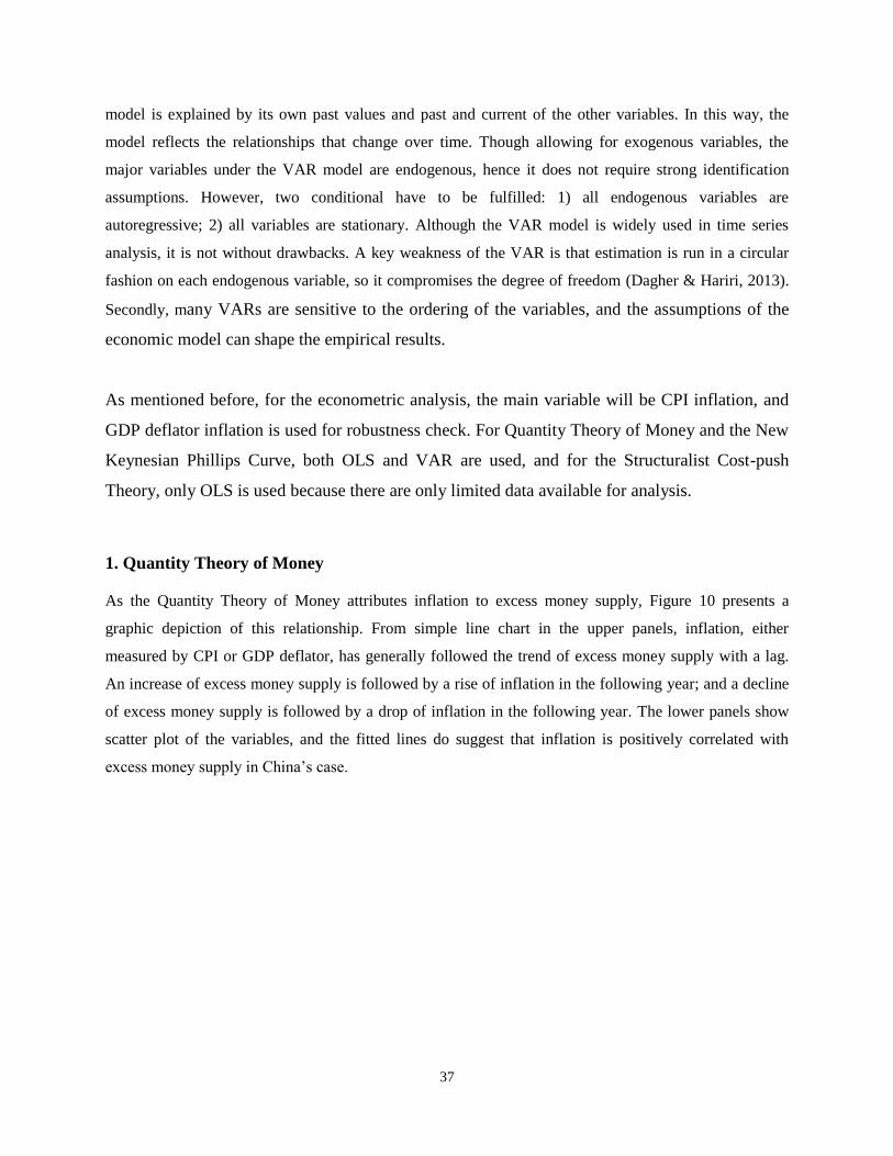
37

model is explained by its own past values and past and current of the other variables. In this way, the

model reflects the relationships that change over time. Though allowing for exogenous variables, the

major variables under the VAR model are endogenous, hence it does not require strong identification

assumptions. However, two conditional have to be fulfilled: 1) all endogenous variables are

autoregressive; 2) all variables are stationary. Although the VAR model is widely used in time series

analysis, it is not without drawbacks. A key weakness of the VAR is that estimation is run in a circular

fashion on each endogenous variable, so it compromises the degree of freedom (Dagher & Hariri, 2013).

Secondly, many VARs are sensitive to the ordering of the variables, and the assumptions of the

economic model can shape the empirical results.

As mentioned before, for the econometric analysis, the main variable will be CPI inflation, and

GDP deflator inflation is used for robustness check. For Quantity Theory of Money and the New

Keynesian Phillips Curve, both OLS and VAR are used, and for the Structuralist Cost-push

Theory, only OLS is used because there are only limited data available for analysis.

1. Quantity Theory of Money

As the Quantity Theory of Money attributes inflation to excess money supply, Figure 10 presents a

graphic depiction of this relationship. From simple line chart in the upper panels, inflation, either

measured by CPI or GDP deflator, has generally followed the trend of excess money supply with a lag.

An increase of excess money supply is followed by a rise of inflation in the following year; and a decline

of excess money supply is followed by a drop of inflation in the following year. The lower panels show

scatter plot of the variables, and the fitted lines do suggest that inflation is positively correlated with

excess money supply in China’s case.

38

Figure 10 Graphic Depiction of Inflation and Excess Money Supply

Note: As discussed in literature review on theories, excess money supply is measured by growth of M2 minus the

growth of real GDP, hence its unit is percentage.

Source: Author.

Table 4 presents the OLS results of the Quantity Theory of Money. Based on the results, Quantity Theory

of Money holds substantial explanatory power over inflation in China, with five out of six regressions

supporting the theory. In regression (c), the year 1998 was significantly negative, which may imply the

impact of external factors such as Asian Financial Crisis and internal factors such as the Price Law. The

year 1994 does not appear to be significant, which indicates that although it is the year of highest inflation,

but it is not a structural break in this model. However, the OLS results should not be over interpreted, as

the underlying data is time series and OLS maybe just capturing a spurious evolution of the two

variables23

.

23

Using Johansen test on time series data, it if found that there is no co-integrating relationship between inflation

and excessive money in the long term.

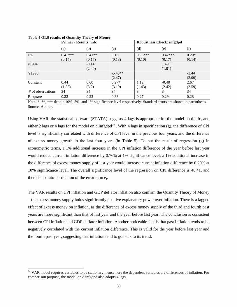
39

Table 4 OLS results of Quantity Theory of Money

Primary Results: infc Robustness Check: infgdpd

(a) (b) (c) (d) (e) (f)

em 0.41***

(0.14)

0.41**

(0.17)

0.16

(0.18)

0.36***

(0.10)

0.42***

(0.17)

0.29*

(0.14)

y1994 -0.14

(2.40)

1.49

(1.81)

Y1998 -5.43**

(2.47)

-1.44

(2.00)

Constant 0.44

(1.88)

0.60

(3.2)

6.27*

(3.19)

1.12

(1.43)

-0.48

(2.42)

2.67

(2.59)

# of observations 34 34 34 34 34 34

R-square 0.22 0.22 0.33 0.27 0.29 0.28

Note: *, **, *** denote 10%, 5%, and 1% significance level respectively. Standard errors are shown in parenthesis.

Source: Author.

Using VAR, the statistical software (STATA) suggests 4 lags is appropriate for the model on d.infc, and

either 2 lags or 4 lags for the model on d.infgdpd24

. With 4 lags in specification (g), the difference of CPI

level is significantly correlated with difference of CPI level in the previous four years, and the difference

of excess money growth in the last four years (in Table 5). To put the result of regression (g) in

econometric terms, a 1% additional increase in the CPI inflation difference of the year before last year

would reduce current inflation difference by 0.76% at 1% significance level; a 1% additional increase in

the difference of excess money supply of last year would increase current inflation difference by 0.20% at

10% significance level. The overall significance level of the regression on CPI difference is 48.41, and

there is no auto-correlation of the error term et.

The VAR results on CPI inflation and GDP deflator inflation also confirm the Quantity Theory of Money

– the excess money supply holds significantly positive explanatory power over inflation. There is a lagged

effect of excess money on inflation, as the difference of excess money supply of the third and fourth past

years are more significant than that of last year and the year before last year. The conclusion is consistent

between CPI inflation and GDP deflator inflation. Another noticeable fact is that past inflation tends to be

negatively correlated with the current inflation difference. This is valid for the year before last year and

the fourth past year, suggesting that inflation tend to go back to its trend.

24

VAR model requires variables to be stationary; hence here the dependent variables are differences of inflation. For

comparison purpose, the model on d.infgdpd also adopts 4 lags.

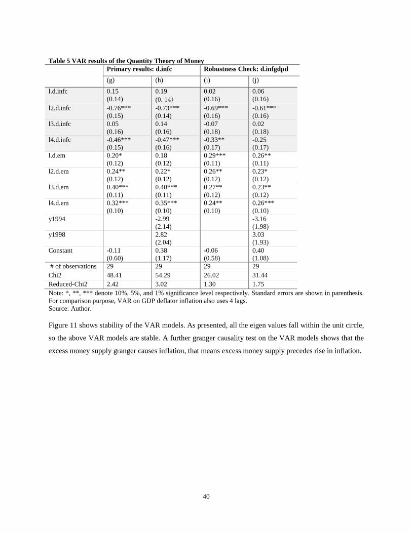
40

Table 5 VAR results of the Quantity Theory of Money

Primary results: d.infc Robustness Check: d.infgdpd

(g) (h) (i) (j)

l.d.infc 0.15

(0.14)

0.19

(0.14)

0.02

(0.16)

0.06

(0.16)

l2.d.infc -0.76***

(0.15)

-0.73***

(0.14)

-0.69***

(0.16)

-0.61***

(0.16)

l3.d.infc 0.05

(0.16)

0.14

(0.16)

-0.07

(0.18)

0.02

(0.18)

l4.d.infc -0.46***

(0.15)

-0.47***

(0.16)

-0.33**

(0.17)

-0.25

(0.17)

l.d.em 0.20*

(0.12)

0.18

(0.12)

0.29***

(0.11)

0.26**

(0.11)

l2.d.em 0.24**

(0.12)

0.22*

(0.12)

0.26**

(0.12)

0.23*

(0.12)

l3.d.em 0.40***

(0.11)

0.40***

(0.11)

0.27**

(0.12)

0.23**

(0.12)

l4.d.em 0.32***

(0.10)

0.35***

(0.10)

0.24**

(0.10)

0.26***

(0.10)

y1994 -2.99

(2.14)

-3.16

(1.98)

y1998 2.82

(2.04)

3.03

(1.93)

Constant -0.11

(0.60)

0.38

(1.17)

-0.06

(0.58)

0.40

(1.08)

# of observations 29 29 29 29

Chi2 48.41 54.29 26.02 31.44

Reduced-Chi2 2.42 3.02 1.30 1.75

Note: *, **, *** denote 10%, 5%, and 1% significance level respectively. Standard errors are shown in parenthesis.

For comparison purpose, VAR on GDP deflator inflation also uses 4 lags.

Source: Author.

Figure 11 shows stability of the VAR models. As presented, all the eigen values fall within the unit circle,

so the above VAR models are stable. A further granger causality test on the VAR models shows that the

excess money supply granger causes inflation, that means excess money supply precedes rise in inflation.

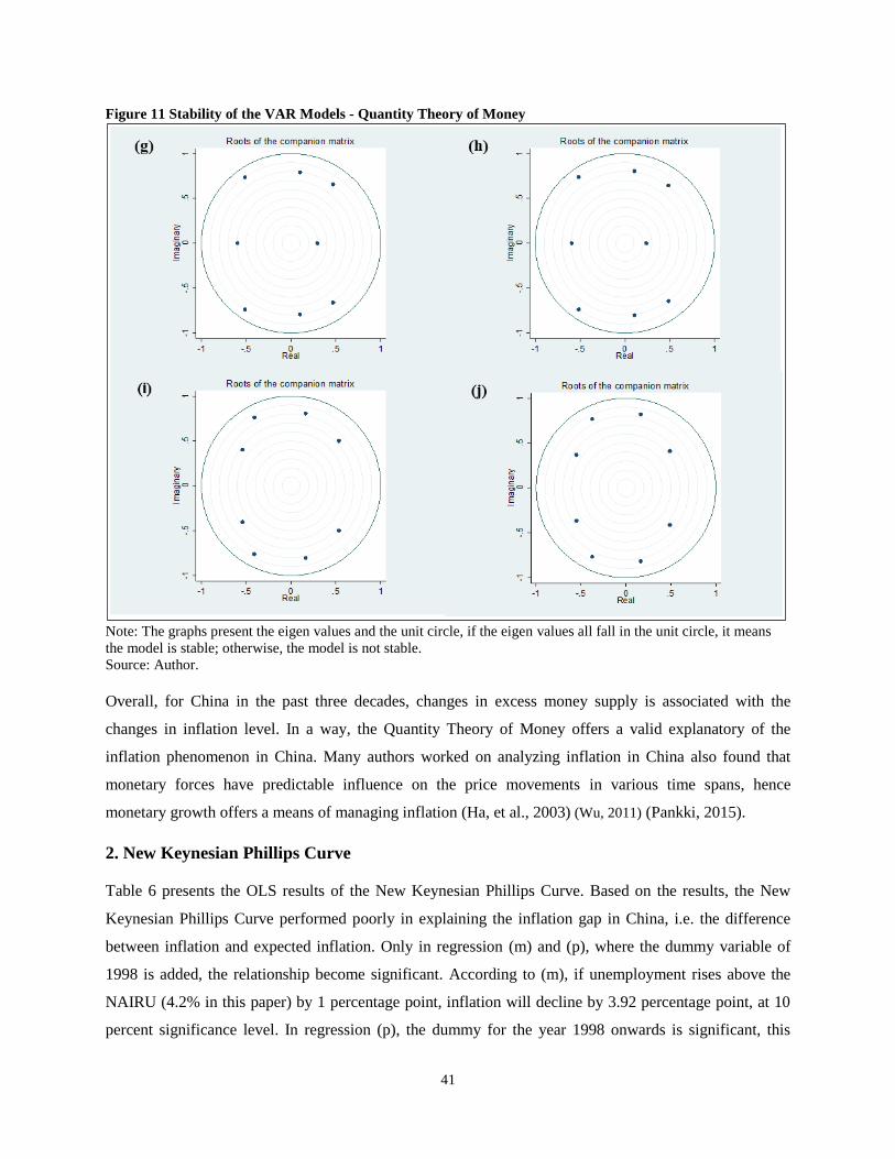
41

Figure 11 Stability of the VAR Models - Quantity Theory of Money

Note: The graphs present the eigen values and the unit circle, if the eigen values all fall in the unit circle, it means

the model is stable; otherwise, the model is not stable.

Source: Author.

Overall, for China in the past three decades, changes in excess money supply is associated with the

changes in inflation level. In a way, the Quantity Theory of Money offers a valid explanatory of the

inflation phenomenon in China. Many authors worked on analyzing inflation in China also found that

monetary forces have predictable influence on the price movements in various time spans, hence

monetary growth offers a means of managing inflation (Ha, et al., 2003) (Wu, 2011) (Pankki, 2015).

2. New Keynesian Phillips Curve

Table 6 presents the OLS results of the New Keynesian Phillips Curve. Based on the results, the New

Keynesian Phillips Curve performed poorly in explaining the inflation gap in China, i.e. the difference

between inflation and expected inflation. Only in regression (m) and (p), where the dummy variable of

1998 is added, the relationship become significant. According to (m), if unemployment rises above the

NAIRU (4.2% in this paper) by 1 percentage point, inflation will decline by 3.92 percentage point, at 10

percent significance level. In regression (p), the dummy for the year 1998 onwards is significant, this

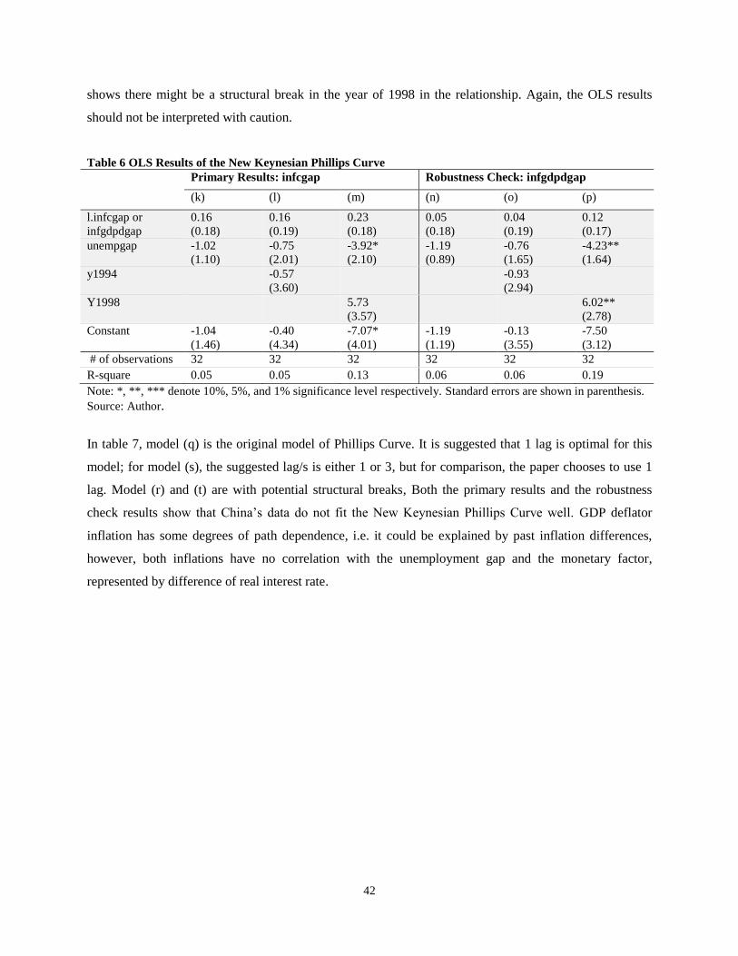
42

shows there might be a structural break in the year of 1998 in the relationship. Again, the OLS results

should not be interpreted with caution.

Table 6 OLS Results of the New Keynesian Phillips Curve

Primary Results: infcgap Robustness Check: infgdpdgap

(k) (l) (m) (n) (o) (p)

l.infcgap or

infgdpdgap

0.16

(0.18)

0.16

(0.19)

0.23

(0.18)

0.05

(0.18)

0.04

(0.19)

0.12

(0.17)

unempgap -1.02

(1.10)

-0.75

(2.01)

-3.92*

(2.10)

-1.19

(0.89)

-0.76

(1.65)

-4.23**

(1.64)

y1994 -0.57

(3.60)

-0.93

(2.94)

Y1998 5.73

(3.57)

6.02**

(2.78)

Constant -1.04

(1.46)

-0.40

(4.34)

-7.07*

(4.01)

-1.19

(1.19)

-0.13

(3.55)

-7.50

(3.12)

# of observations 32 32 32 32 32 32

R-square 0.05 0.05 0.13 0.06 0.06 0.19

Note: *, **, *** denote 10%, 5%, and 1% significance level respectively. Standard errors are shown in parenthesis.

Source: Author.

In table 7, model (q) is the original model of Phillips Curve. It is suggested that 1 lag is optimal for this

model; for model (s), the suggested lag/s is either 1 or 3, but for comparison, the paper chooses to use 1

lag. Model (r) and (t) are with potential structural breaks, Both the primary results and the robustness

check results show that China’s data do not fit the New Keynesian Phillips Curve well. GDP deflator

inflation has some degrees of path dependence, i.e. it could be explained by past inflation differences,

however, both inflations have no correlation with the unemployment gap and the monetary factor,

represented by difference of real interest rate.

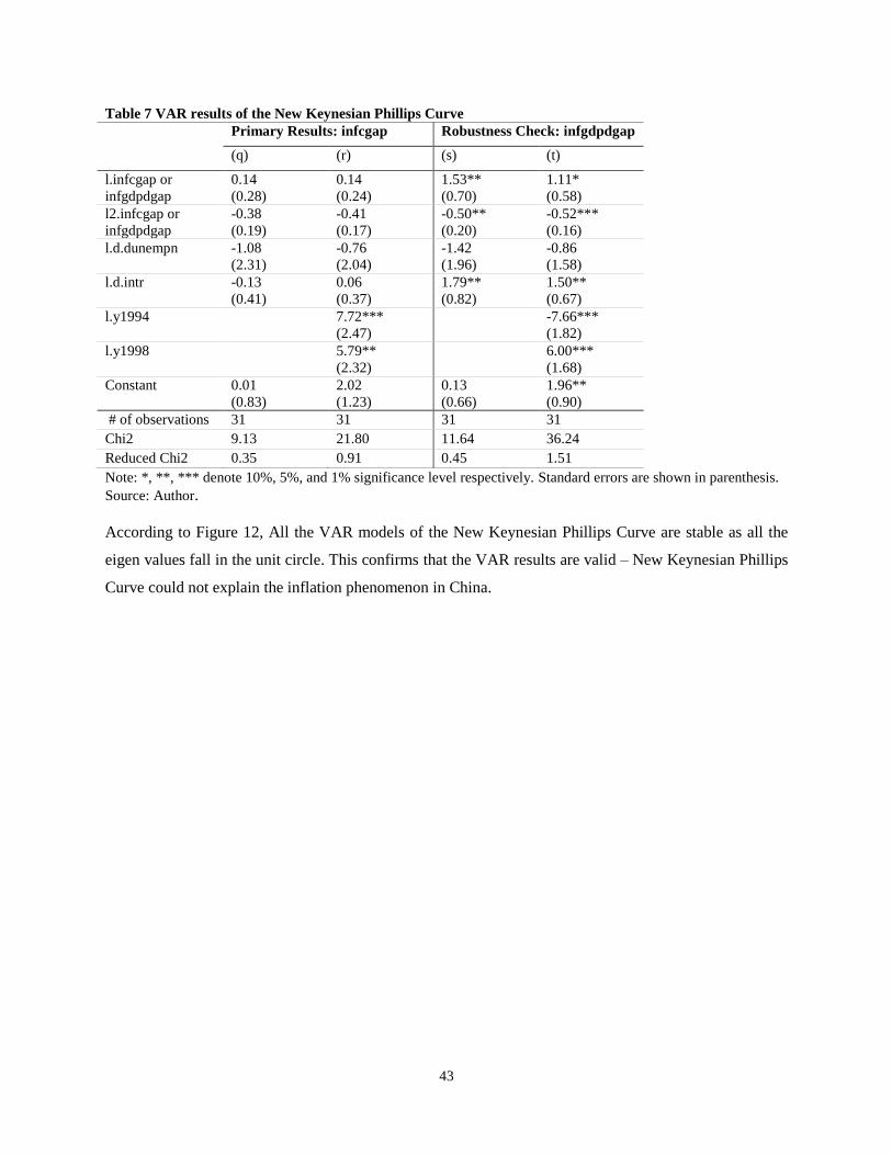
43

Table 7 VAR results of the New Keynesian Phillips Curve

Note: *, **, *** denote 10%, 5%, and 1% significance level respectively. Standard errors are shown in parenthesis.

Source: Author.

According to Figure 12, All the VAR models of the New Keynesian Phillips Curve are stable as all the

eigen values fall in the unit circle. This confirms that the VAR results are valid – New Keynesian Phillips

Curve could not explain the inflation phenomenon in China.

Primary Results: infcgap Robustness Check: infgdpdgap

(q) (r) (s) (t)

l.infcgap or

infgdpdgap

0.14

(0.28)

0.14

(0.24)

1.53**

(0.70)

1.11*

(0.58)

l2.infcgap or

infgdpdgap

-0.38

(0.19)

-0.41

(0.17)

-0.50**

(0.20)

-0.52***

(0.16)

l.d.dunempn -1.08

(2.31)

-0.76

(2.04)

-1.42

(1.96)

-0.86

(1.58)

l.d.intr -0.13

(0.41)

0.06

(0.37)

1.79**

(0.82)

1.50**

(0.67)

l.y1994 7.72***

(2.47)

-7.66***

(1.82)

l.y1998 5.79**

(2.32)

6.00***

(1.68)

Constant 0.01

(0.83)

2.02

(1.23)

0.13

(0.66)

1.96**

(0.90)

# of observations 31 31 31 31

Chi2 9.13 21.80 11.64 36.24

Reduced Chi2 0.35 0.91 0.45 1.51

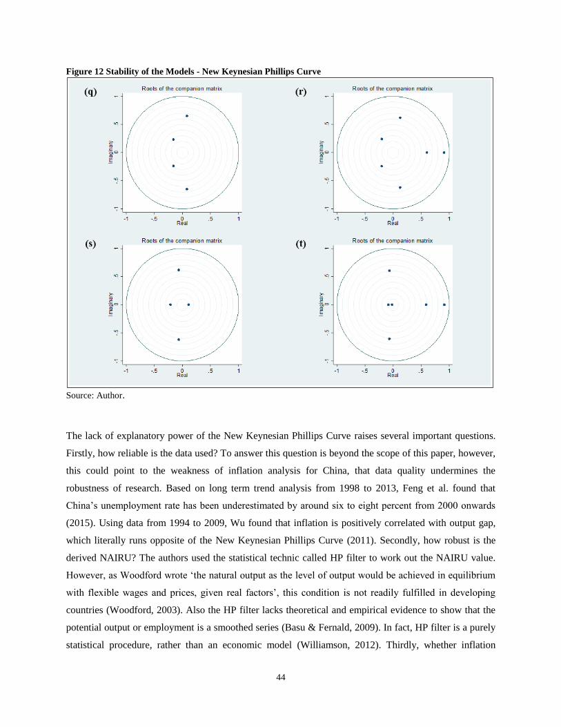
44

Figure 12 Stability of the Models - New Keynesian Phillips Curve

Source: Author.

The lack of explanatory power of the New Keynesian Phillips Curve raises several important questions.

Firstly, how reliable is the data used? To answer this question is beyond the scope of this paper, however,

this could point to the weakness of inflation analysis for China, that data quality undermines the

robustness of research. Based on long term trend analysis from 1998 to 2013, Feng et al. found that

China’s unemployment rate has been underestimated by around six to eight percent from 2000 onwards

(2015). Using data from 1994 to 2009, Wu found that inflation is positively correlated with output gap,

which literally runs opposite of the New Keynesian Phillips Curve (2011). Secondly, how robust is the

derived NAIRU? The authors used the statistical technic called HP filter to work out the NAIRU value.

However, as Woodford wrote ‘the natural output as the level of output would be achieved in equilibrium

with flexible wages and prices, given real factors’, this condition is not readily fulfilled in developing

countries (Woodford, 2003). Also the HP filter lacks theoretical and empirical evidence to show that the

potential output or employment is a smoothed series (Basu & Fernald, 2009). In fact, HP filter is a purely

statistical procedure, rather than an economic model (Williamson, 2012). Thirdly, whether inflation

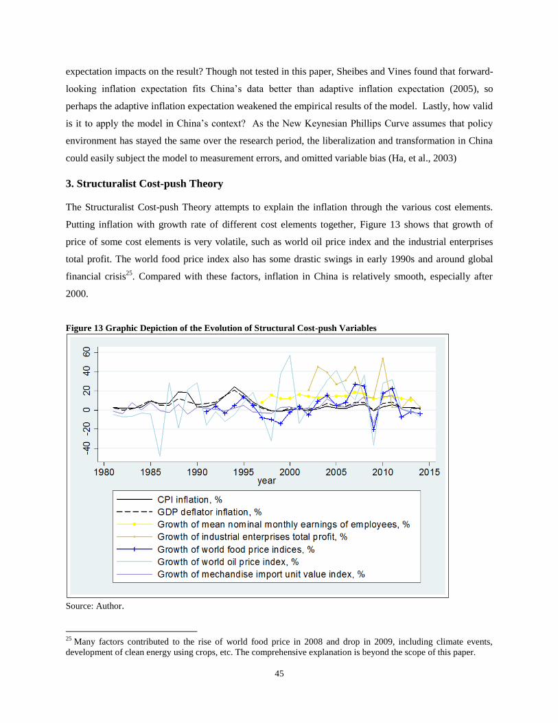
45

expectation impacts on the result? Though not tested in this paper, Sheibes and Vines found that forward-

looking inflation expectation fits China’s data better than adaptive inflation expectation (2005), so

perhaps the adaptive inflation expectation weakened the empirical results of the model. Lastly, how valid

is it to apply the model in China’s context? As the New Keynesian Phillips Curve assumes that policy

environment has stayed the same over the research period, the liberalization and transformation in China

could easily subject the model to measurement errors, and omitted variable bias (Ha, et al., 2003)

3. Structuralist Cost-push Theory

The Structuralist Cost-push Theory attempts to explain the inflation through the various cost elements.

Putting inflation with growth rate of different cost elements together, Figure 13 shows that growth of

price of some cost elements is very volatile, such as world oil price index and the industrial enterprises

total profit. The world food price index also has some drastic swings in early 1990s and around global

financial crisis25

. Compared with these factors, inflation in China is relatively smooth, especially after

2000.

Figure 13 Graphic Depiction of the Evolution of Structural Cost-push Variables

Source: Author.

25

Many factors contributed to the rise of world food price in 2008 and drop in 2009, including climate events,

development of clean energy using crops, etc. The comprehensive explanation is beyond the scope of this paper.

46

For Structuralist Cost-push Theory, regression is only run using OLS26

. Table 8 presents the primary

results and Table 9 the results of robustness check. Table 8 shows the trade-off between the number of

variables included and the number of years covered – the more variables are included, the less years of

data are available. The overall results show that the year 1998 did appear as a structural break in data,

because when the variable is included, it is significantly negative. In latter regressions, due to limited

years of data, y1998 could not be included.

Among all the variables, food price level, either world or domestic, tend to have significant explanatory

power of inflation; especially domestic food price level, a 1 percent growth of domestic food price is

associated with a 0.91 percent increase in inflation difference, at 1 percent significance level. This is quite

a large impact. This might be associated with how CPI is constructed, though the exact weight of food in

CPI basket is unknown, but it does occupy a substantial representation.

As for other variables, they are occasionally significant, but they do not show consistency in their

influence on inflation. The world oil price fails in explain the inflation in China; this might be ‘due to the

strict control of oil price, there is no direct linkage between world oil price and the overall price level in

China’ (Chen, 2008). It is possible that non-significant import price level could also be explained in this

way. It is noteworthy that although less years of data are used, the latter regressions do have a higher

explanatory power then earlier ones. One reason for this is more variables are used in latter regressions,

and the other reason might be data quality is better in later years.

26

As mentioned in the beginning of this sub-section, using OLS only is because for some variables of the cost-push

model, there are only 14 years of data. Given VAR tend to have lag/s, the data is too few to derive valid results.

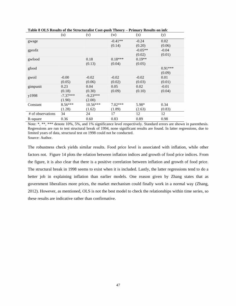
47

Table 8 OLS Results of the Structuralist Cost-push Theory – Primary Results on infc

(u) (v) (w) (x) (y)

gwage -0.41**

(0.14)

-0.24

(0.20)

0.02

(0.06)

gprofit -0.05**

(0.02)

-0.04

(0.01)

gwfood 0.18

(0.13)

0.18***

(0.04)

0.19**

(0.05)

gfood 0.91***

(0.09)

gwoil -0.00

(0.05)

-0.02

(0.06)

-0.02

(0.02)

-0.02

(0.03)

0.01

(0.01)

gimpunit 0.23

(0.18)

0.04

(0.30)

0.05

(0.09)

0.02

(0.10)

-0.01

(0.04)

y1998 -7.37***

(1.90)

-9.23***

(2.00)

Constant 8.56***

(1.28)

10.56***

(1.62)

7.02***

(1.89)

5.98*

(2.63)

0.34

(0.83)

# of observations 34 24 17 12 12

R-square 0.36 0.60 0.83 0.89 0.98

Note: *, **, *** denote 10%, 5%, and 1% significance level respectively. Standard errors are shown in parenthesis.

Regressions are run to test structural break of 1994, none significant results are found. In latter regressions, due to

limited years of data, structural test on 1998 could not be conducted.

Source: Author.

The robustness check yields similar results. Food price level is associated with inflation, while other

factors not. Figure 14 plots the relation between inflation indices and growth of food price indices. From

the figure, it is also clear that there is a positive correlation between inflation and growth of food price.

The structural break in 1998 seems to exist when it is included. Lastly, the latter regressions tend to do a

better job in explaining inflation than earlier models. One reason given by Zhang states that as

government liberalizes more prices, the market mechanism could finally work in a normal way (Zhang,

2012). However, as mentioned, OLS is not the best model to check the relationships within time series, so

these results are indicative rather than confirmative.

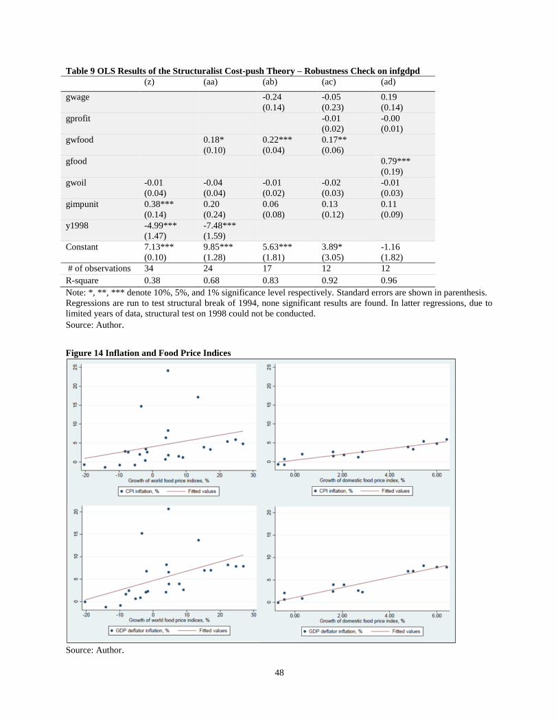
48

Table 9 OLS Results of the Structuralist Cost-push Theory – Robustness Check on infgdpd

(z) (aa) (ab) (ac) (ad)

gwage -0.24

(0.14)

-0.05

(0.23)

0.19

(0.14)

gprofit -0.01

(0.02)

-0.00

(0.01)

gwfood 0.18*

(0.10)

0.22***

(0.04)

0.17**

(0.06)

gfood 0.79***

(0.19)

gwoil -0.01

(0.04)

-0.04

(0.04)

-0.01

(0.02)

-0.02

(0.03)

-0.01

(0.03)

gimpunit 0.38***

(0.14)

0.20

(0.24)

0.06

(0.08)

0.13

(0.12)

0.11

(0.09)

y1998 -4.99***

(1.47)

-7.48***

(1.59)

Constant 7.13***

(0.10)

9.85***

(1.28)

5.63***

(1.81)

3.89*

(3.05)

-1.16

(1.82)

# of observations 34 24 17 12 12

R-square 0.38 0.68 0.83 0.92 0.96

Note: *, **, *** denote 10%, 5%, and 1% significance level respectively. Standard errors are shown in parenthesis.

Regressions are run to test structural break of 1994, none significant results are found. In latter regressions, due to

limited years of data, structural test on 1998 could not be conducted.

Source: Author.

Figure 14 Inflation and Food Price Indices

Source: Author.

49

Due to data limitations, the paper can only go this far to interpret the factors. However, there are other

authors using different technics identified that wage growth, raw material prices, international oil price,

food price, the world price level, etc. are important determinants of price level in China (Ha, et al., 2003)

(Kojima, et al., 2005) (Jongwanich & Park, 2008). There are also authors cautioned that the results of

cost-push research are often specific to various methodological choices and data definitions (Peneva &

Rudd, 2015).

IV. Summary

The paper applied different theories on inflation data in China, the results show that Quantity Theory of

Money does have significant explanatory power of the inflation, while New Keynesian Phillips Curve

performed poorly in explaining inflation movement. Due to data limitations, only the food price level

under the Cost-push Theory holds positive influence on inflation, while all the other factors do not seem

to correlated with inflation. Regarding structural breaks, the year 1998 appears to be a break point;

however, this conclusion is not consistent across all the models.

There are several issues that are not covered in the analysis that can potentially change the above

conclusion. Firstly, as mentioned a number of times, data availability and quality impose severe constraint

on the analysis. Given the scarcity of data, it’s not possible to check on measurement errors or test

omitted variables, hence data constraint becomes a major weakness of econometric analysis. Secondly, all

three models specify a linear relationship between inflation and explanatory variables, however, the

relationship could be in other shapes in reality. As Bruno and Easterly mentioned ‘it seemed implausible

that an additional 100 percentage points of inflation meant the same at 0 as it meant at 1,000. But attempts

at spline regressions are extremely sensitive to the one or two points in the relevant intermediate ranges’

(Bruno & Easterly, 1996). Thirdly, the endogeneity of the variables may disguise the true relation. As

Mankiw said: ‘Correlations among endogenous variables can rule out theories that fail to produce the

correlations, and they can thereby raise our confidence in theories that do produce them’ (Asymptosis,

2008), so it is hard to ascertain that the results from above regression are valid and robust.

50

Chapter 5: Conclusion

‘Stable prices provide a sense of security. They help define a reliable social and political order.

They are like safe streets, clean drinking water and dependable electricity. Their importance is

noticed only when they go missing.’ (Samuelson, 2008)

This paper studied China’s inflation based on yearly data of related factors in the past three decades. It

examined the nature and causes of inflation evolution in China. Adopting a relatively comprehensive

approach, the paper put together a background that covers definition, measurement, policy factors and

empirical trends of inflation, and studied in-depth the three major schools of theory on inflation and

examined the causes of inflation in China from these three major theoretical angles.

A tradeoff to this comprehensive approach is that the paper is unable to go in-depth in discussing how

each theory is applied in developing countries, and to present an interrogation of each literature that

applies the theory in China’s context.

From descriptive analysis, the paper found that the inflation evolution in China is not a straight-forward

process. It presents a confluence of many factors, including monetary policy, price liberalization,

exchange rate policy, progress of broader economic reform, external shocks and the learning process of

the PBOC.

The econometric analysis offers key insights into the story behind data, i.e. the causes of the inflation in

China. Comparing the three theories, the findings indicated that from demand pull perspective, the

Quantity Theory of Money provides a sensible explanation of inflation trends in China, while the New

Keynesian Phillips Curve does not fit the data on inflation; and from cost push perspective, the

Structuralist Cost-push Theory did identify the correlation between inflation trend and food price

movement, while none of the other factors matter.

The results, in a way is aligned with quite a large number of literatures, which find Quantity Theory of

Money is the primary theory that guide the monetary operation in China. Food price could explain

inflation is primarily because it consist a substantial portion of inflation basket, so logically it holds

explanatory power. The econometric analysis also identify that the year 1998 is a potential structural

break in inflation evolution.

51

In retrospect, the paper confirmed the hypothesis that inflation in China is largely driven by excess

money supply, and is correlated with changes in food price level. From demand-pull perspective, the

Quantity Theory of Money appears to be superior than the New Keynesian Philips Curve, and the Cost-

push Theory also accounts for the inflation phenomenon to some extent. In the long run, the Quantity

Theory of Money and the Cost-push Theory should be given equal consideration as theoretical grounds to

manage inflation in China.

52

References

Adalid, R. & Detken, C., 2007. Liquidity Shocks and Asset Price Boom/Bust Cycles, ECB Working

Paper No732. Frankfurt, European Central Bank.

Addison, J. & Burton, J., 1980. The Demise of 'Demand-pull' and 'Cost-push' in Inflation Theory.

PSL Quarterly Review, 33(133), pp. 187-203.

Aidar, G., 2012. The New Keynesian Phillips Curve: a Critical Assessment. Brazilian Development

Bank Working Paper, pp. 1-33.

Alimi, S., 2012. The Quantity Thoery of Money and its Long-run Implications: Empirical Evidence

from Nigeria. European Scientific Journal, 8(12), pp. 272-288.

Apergis, N., Miller, S., Panethimitakis, A. & Vamvakidis, A., 2005. Inflation Targeting and Output

Growth: Evidence from Aggregate European Data. s.l., University of Connecticut.

Asymptosis, 2008. Mankiw: Post Friedman Ergo Propter Friedman. [Online]

Available at: http://www.asymptosis.com/mankiw-post-friedman-ergo-propter-friedman.html

[Accessed 15 September 2016].

Atkeson, A., 2001. Are Phillips Curves Useful for Forecasting Inflation?. Federal Reserve Bank of

Minneapolis, 25(1), pp. 2-11.

Ball, L. & Mankiw, G., 2002. The NAIRU in Theory and Practice. Journal of Economic Perspectives,

16(4), pp. 115-136.

Banque de France, 2009. Deflation or Disinflation?. Focus, 22 January, pp. 1-4.

Basu, S. & Fernald, J., 2009. What do We Know (and not Know) about Potential Output?. Federal

Reserve Bank of St. Louis Review, 91(4), pp. 187-213.

Batten, D., 1981. Inflation: the Cost-Push Myth. Federal Reserve Bank of St. Louis, June/July, pp. 21-

26.

Benes, J. & N'Diaye, P., 2004. A Multivariate Filter for Measuring Potential Output and the NAIRU:

Application to the Czech Republic, Washington D.C.: IMF.

Benhabib, J., Schmitt-Grohe, S. & Uribe, M., 2002. Avoiding Liquidity Traps. Journal of Political

Economy, Volume 110, pp. 535-563.

Bernstein, J. & Baker, D., 2013. CPER: The Unemployment Rate at Full Employment: How Low can

You Go?. [Online]

Available at: http://cepr.net/publications/op-eds-columns/the-unemployment-rate-at-full-employment-

how-low-can-you-go

[Accessed 24 June 2016].

53

Blinder, A., 1997. Is There a Core of Practical Macroeconomics that We should All Believe?.

American Economic Review , Volume 87, pp. 240-243.

Brissimis, S. & Magginas, N., 2008. Inflation Forecasts and the New Keynesian Phillips Curve.

International Journal of Central Banking, 4(2), pp. 1-22.

Broda, C. & Weinstein, D., 2004. Variety Growth and World Welfare. The American Economic

Review, 94(2), pp. 139-144.

Brue, S. L., 2000. The Neoclassical School - Monetary Economics. In: C. Goldfinch, ed. The

Evolution of Economic Thought. Mason, Ohio: Thomson South-Western, pp. 322-341.

Bruno, M. & Easterly, W., 1996. Inflation and Growth: In Search of a Stable Relationship. St. Louis,

Federal Reserve Bank of St. Louis.

Burdekin, R. & Siklos, P., 2008. What has driven Chinese monetary policy since 1990? Investigating

the People's Bank's Policy Rule. Journal of International Money and Finance, Volume 27, pp. 847-

859.

Calvo, G., 1983. Staggered Prices in a Utility Maximizing Framework. Journal of Monetary

Economics, Volume 12, pp. 383-398.

Calvo, G., 1983. Staggered Prices in a Utility-Maximizing Framework. Journal of Monetary

Economics, 12(3), pp. 383-398.

Chen, Y., 2008. Research on New Keynesian Phillips Curve in China. Economic Research, Volume

12, pp. 50-64.

Chen, Y., 2008. The Empirical Study of China Current Inflation's Causes: 2003-2007. Economic

Theories and Economic Management, Volume 2, pp. 16-22.

China National Bureau of Statistics , 2016. National Data. [Online]

Available at: http://data.stats.gov.cn/easyquery.htm?cn=C01

[Accessed 26 July 2016].

China National Bureau of Statistics, 2009. CPI Data Publication Timing and Content. [Online]

Available at: http://www.stats.gov.cn/ztjc/tjzs/cpizzg/200902/t20090219_67277.html

[Accessed 14 May 2016].

China National Bureau of Statistics, 2009. CPI Representative Items and Weights. [Online]

Available at: http://www.stats.gov.cn/ztjc/tjzs/cpizzg/200902/t20090219_67274.html

[Accessed 15 May 2016].

China National Bureau of Statistics, 2011. Major Statistical Index and Explanation. [Online]

Available at: http://www.stats.gov.cn/tjsj/ndsj/2012/html/zb24.htm

[Accessed 10 October 2016].

54

China National Bureau of Statistics, 2011. The Relation between Inflation and CPI. [Online]

Available at: http://www.stats.gov.cn/ztjc/tjzs/zjcpi/201106/t20110613_71512.html

[Accessed 30 10 2016].

China National Bureau of Statistics, 2011. What is Inflation?. [Online]

Available at: http://www.stats.gov.cn/ztjc/tjzs/zjcpi/201106/t20110610_71467.html

[Accessed 14th May 2015].

China National Bureau of Statistics, 2016. National Data. [Online]

Available at: http://data.stats.gov.cn/easyquery.htm?cn=C01

[Accessed 20 August 2016].

Christensen, M., 2001. Real Supply Shocks and the Money Growth - Inflation Relationship.

Economics Letters, 72(1), pp. 67-72.

Cogley, T. & Sbordone, A., 2008. Trend Inflation, Indexation, and Inflation Persistence in the New

Keynesian Phillips Curve. American Economic Review, 98(5), pp. 2101-2126.

Crowder, W., 1998. The Long-run Link between Money Growth and Inflation. Economic Inquiry,

36(2), pp. 229-243.

Dagher, L. & Hariri, S., 2013. The Impact of Global Oil Price Shocks on the Lebanese Stock Market.

Energy, Volume 63, pp. 366-374.

Dai, G., 2002. China's Monetary Policy: Too Tight?. China and World Economy, Volume 5, pp. 16-

20.

De Brouwer, G. & Ericsson, N., 1995. Modelling Inflation in Australia, Canberra: Reserve Bank of

Australia.

De Grauwe, P. & Polan, M., 2005. Is Inflation Always and Everywhere a Monetary Phenomenon?.

The Scandinavian Journal of Economics, 107(2), pp. 239-259.

DeLong, B., 1996. America’s Peacetime Inflation: the 1970s.. In: C. Romer & D. Romer, eds.

Reducing Inflation: Motivation and Strategy. Chicago: University of Chicago Press, pp. 247-280.

Dreger, C. & Zhang, Y., 2011. The Chinese Impact on GDP Growth and Inflation in the Industrial

Countries. Berlin, Deutsches Institut fur Wirtschafsforschung.

Du, Y. & Lu, Y., 2009. China's Nature Unemployment and Phillips Curve: 1987-2008, Beijing:

Chinese Academy of Social Sciences, Population and Labor Economics Institute.

Du, Y. & Lu, Y., 2011. The Natural Rate of Unemployment in China: Estimation, Compositiono, and

Implication. The World Economy , Volume 4, pp. 3-21.

Emerson, J., 2006. The Quantity Theory of Money: Evidence from teh United States. Economic

Bulletin, 5(2), pp. 1-6.

55

Espinosa, M. & Russell, S., 1997. History and Theory of the NAIRU: A Critical Review. Federal

Reserve Bank of Atlanta Economic Review, Issue 2, pp. 4-25.

Fabiani, S. & Mestre, R., 2000. Alternative Measures of the NAIRU in the Euro Area: Estimates and

Assessment, Frankfurt: European Central Bank.

Fabiani, S. & Mestre, R., 2001. A System Approach for Measuring the Euro Area NAIRU. European

Central Bank Working Paper, Volume 65.

Fan, L., Yu, Y. & Zhang, C., 2011. An Empirical Evaluation of China's Monetary Policies. Journal of

Macroeconomics, 33(2), pp. 358-371.

Fan, Z., 2008. Is China's Inflation a Wage Cost-push?. China Macroeconomic Analysis and

Forecasting, Volume mid-year, pp. 1-19.

Fan, Z., 2010. Cost-push Inflation - Meaning, Identification and Anti-inflation Policies. World

Economy Volume 1, pp. 123-132.

Feng, S., Hu, Y. & Moffitt, R., 2015. Long Run Trends in Unemployment and Labor Force

Participation in China. Washington D.C., NBER Working Paper No.21460.

Fisher, I., 1911. The Purchasing Power of Money. 2nd edition ed. New York: Macmillan.

Fisher, I., 1912. The Purchasing Power of Money: Its Determination and Relation to Credit Interest

and Crises. 2nd ed. New York: Macmillan Company.

Food and Agriculture Organization of United Nations, 2016. World Food Situation - Food Price

Index. [Online]

Available at: http://www.fao.org/worldfoodsituation/foodpricesindex/en/

[Accessed 29 August 2016].

Friedman, M., 1968. The Role of Monetary Policy. The American Economic Review, LVIII(1), pp. 1-

17.

Friedman, M., 1970. A Theoretical Framework for Monetary Analysis. Journal of Political Economy,

78(2), pp. 193-238.

Friedman, M., 1977. Nobel Lecture: Inflation and Unemployment. The Journal of Political Economy,

85(3), pp. 451-472.

Friedman, M. & Schwartz, A., 1982. The General Theoretical Framework. In: N. B. o. E. Research,

ed. Monetary Trends in the United States and United Kingdom: Their Relation to Income, Prices, and

Interest Rates, 1867-1975. Chicago: University of Chicago Press, pp. 16-72.

Fuhrer, J., 1995. The Phillips Curve is Alive and Well. New England Economic Review, March/April,

pp. 41-56.

Funke, M., 2006. Inflation in Mainland China – Modelling a Roller Coaster Ride, BOFIT Discussion

Paper No6/2005. Munich, Center for Economic Studies and IfoInstitute.

56

Fu, Q., Zhu, Y. & Yuan, C., 2011. Estimation and Explanation on Main Influencing Factors of

Inflation in China. China Industrial Economics, Volume 05, p. 3.

Gali, J. & Gertler, M., 1999. Inflation Dynamics: a Structural Economic Analysis. Journal of

Monetary Economics , Volume 44, pp. 195-222.

Gehringer, A., 2015. Monetary Policy Made in China, Koln: Flossbach von Storch Research Institute.

Geiger, M., 2008. Instruments of Monetary Policy in China and Their Effectiveness: 1994-2006,

Geneva: United Nations Conference on Trade and Development.

Gerlach, S. & Peng, W., 2006. Output Gaps and Inflation in Mainland China. China Economic

Review, 17(2), pp. 210-225.

Gibbs, D., 1995. Potential Output: Concepts and Measurement. Labour Market Bulletin, Volume 1,

pp. 72-115.

Goldstein, M. & Lardy, N., 2007. China’s Exchange Rate Policy: An Overview of Some Key Issues.

Washington D.C., Peterson Institute of International Economics.

Goodfriend, M. & Prasad, E., 2011. A Framework for Independent Monetary Policy in China.

Washington D.C., International Monetary Fund .

Gordon, R., 1997. The Time-varying NAIRU and its Implications for Economic Policy. Journal of

Economic Perspectives, 11(1), pp. 11-32.

Greenslade, J., Pierse, R. & Saleheen, J., 2003. A Kalman Filter Approach to Estimating the UK

NAIRU. Bank of Englang Working Paper, Volume 179.

Gregory, M. N., 2009. Chapter 17 Money Growth and Inflation. In: M. N. Gregory, ed. Principles of

Macroeconomics. Boston: South-Western Cengage Learning, p. 464.

Guerineau, S. & Guillamont, S., 2005. Deflation in China. China Economic Review, 16(4), pp. 336-

363.

Haberler, G., 1960. Inflation: its Causes and Cures. Washington D.C.: American Enterprise

Association.

Ha, J., Fan, K. & Shu, C., 2003. The Causes of Inflation and Deflation in Mainland China. Hong

Kong Monetary Authority Quarterly Bulletin, September , pp. 23-31.

Hansen, B., 1951. A Study in the Theory of Inflation. Abingdon and New York: Routledge.

Harvey, J., 1991. A Post Keynesian View of Exchange Rate Determination. Journal of Post

Keynesian Economics, 14(1), pp. 61-71.

Herz, B. & Roeger, W., 2012. Traditional versus New Keynesian Phillips Curves: Evidence from

Output Effects. International Journal of Central Banking , 8(2), pp. 87-109.

Higgins, B., 1978. Velocity: Money's Second Dimension. Economic Review, Volume June, pp. 15-31.

57

Holzman, F. D., 1960. Inflation: Cost-Push and Demand-Pull. The American Economic Review, 50(1),

pp. 20-42.

Humphrey, T., 1974. The Quantity Theory of Money: Its Historical Evolution and Role in Policy

Debates. Federal Reserve Bank Richmond Economic Review, 60(May/June), pp. 2-19.

Humphrey, T., 1976. On Cost-push Theories of Inflation in the Pre-War Monetary Literature. PSL

Quarterly Review, 29(116), pp. 77-89.

Humphrey, T., 1998. Historical Origins of the Cost-push Fallacy. Federal Reserve Bank of Richmond

Economic Quarterly, 84(3), pp. 53-74.

IMF, 2016. Dissemination Standards Bulletin Board - Special Data Dissemination Standard. [Online]

Available at: http://dsbb.imf.org/Pages/SDDS/CustomizedQuery/ByARC.aspx

[Accessed 15 May 2016].

International Labor Organization, 2016. ILO Statistics and Databases. [Online]

Available at: http://www.ilo.org/ilostat/faces/help_home?_adf.ctrl-

state=o6ebzwxa6_4&_afrLoop=351392616628373#!

[Accessed 25 August 2016].

International Monetary Fund, 2003. Deflation: Determinants, Risks, and Policy Options - Findings of

an Interdepartmental Task Force, Washington, D.C.: International Monetary Fund.

International Monetary Fund, 2016. International Finance Statistics. [Online]

Available at: http://www.imf.org/external/pubs/cat/longres.aspx?sk=20095

[Accessed 26 August 2016].

International Monetary Fund, 2016. World Economic Outlook: Subdued Demand Symptoms and

Remedies, Washington D.C.: IMF.

Javed, Z. H. & Akram, S., 2010. Impact of Cost-push and Monetary Factors on Wholesale Price

Index: Empirical Evidence from the Economy of Pakistan. s.l., International Conference on Applied

Economics.

Jiang, C., Chang, T. & Li, X., 2015. Money Growth and Inflation in China: New Evidence from a

Wavelet Analysis. International Review of Economics and Finance, Volume 35, pp. 249-261.

Jongwanich, J. & Park, D., 2008. Inflation in Developing Asia: Demand-pull or Cost-Push?, Manila:

Asian Development Bank.

Kaldor, N., 1986. The Scourge of Monetarism. Oxford: Oxford University Press.

Keynes, J. M., 1964. The General Theory of Employment, Interest, and Money. New York: Atlantic

Publishers and Distributors LTD.

Koch-Weser, I., 2013. The Reliability of China’s Economic Data: an Analysis of National Output,

Washington D.C.: U.S.-China Economic and Security Review Comission.

58

Kojima, R., Nakamura, S. & Ohyama, S., 2005. Inflation Dynamics in China, Bank of Japan Working

Paper 5-E. Japan, Bank of Japan.

Koutun, A. & Karabona, P., 2013. An Empirical Study of the Solow Growth Model, s.l.: Malardalen

University Sweden.

Lin, J. Y., 2004. Lessons of China's Transition from a Planned Economy to a Market Economy.

Warsaw, Leon Kozminsi Academy of Entrepreneurship and Management.

Liu, B. & Zhang, H., 2001. Estimation of China's Output Gap. Finance Research, Volume 10, pp. 69-

77.

Liu, G. & Chen, D., 2012. A Study on Relationship between Inflation and Money Supply from an

Endogenous Perspective. Economic Perspectives, Volume 8, pp. 51-56.

Liu, H. & Jiang, G., 2009. Explaining Causes of China's Inflation - Theoretical Framework and

Empirical Research. Research on Quantitative Economics and Technical Economics, Volume 1, pp.

77-88.

Liu, L. & Zhang, W., 2010. A New Keynesian Model for Analysing Monetary Policy in Mainland

China. Journal of Asian Economics, 21(6), pp. 540-551.

Llaudes, R., 2005. The Phillips Curve and Long-term Unemployment. European Central Bank

Working Paper Series, February, pp. 1-49.

Lucas, R., 1972. Expectations and the Neutrality of Money. Journal of Economic Theory, 4(2), pp.

103-124.

Lucas, R. E. J., 1972. Expectations and the Neutrality of Money. Journal of Economic Theory,

Volume 4, pp. 103-124.

Lu, F. & Hou, J., 2013. An Analysis of Dynamic Effect of Influence Factors of Inflation in China.

Commercial Research, Volume 5, p. 2.

Majumder, A., 2006. Inflation in Bangladesh: Supply Side Perspectives, Dhaka: Bangladesh Bank.

Makochekanwa, A., 2007. A Dynamic Enquiry into the Causes of Hyperinflation in Zimbabwe.

Transport, Volume 9, pp. 1-31.

Mankiw, G., 1997. macroeconomics. 3 ed. New York: Worth Publishing.

Mankiw, G., 2001. The Inexorable and Mysterious Tradeoff between Inflation and Unemployment.

The Economic Journal, 111(471), pp. 45-61.

Mankiw, G., 2015. Chapter 30 Money Growth and Inflation. In: G. Mankiw, ed. Principles of

Economics. Stamford: Cengage learning, pp. 633-654.

Manning, N., 1994. Are Higher Long-term Unemployment Rate Associated with Lower Earnings?.

Oxford Bulletin of Economics and Statistics, 56(4), pp. 387-397.

59

Ma, Y., 2014. Monetary Policy Based on Non-linear Quantity Rule: Evidence from China.

International Review of Economics and Finance, Volume 34, pp. 89-104.

MBAlib, 2014. MBAlib - Retail Price Index. [Online]

Available at:

http://wiki.mbalib.com/wiki/%E9%9B%B6%E5%94%AE%E7%89%A9%E4%BB%B7%E6%8C%8

7%E6%95%B0

[Accessed 10 June 2016].

McCallum, B., 1988. Robustness Properties of a Rule for Monetary Policy. Carnegie-Rochester

Conference Series on Public Policy, Volume 29, pp. 173-203.

McCallum, B., 1997. Crucial Issues Concerning Central Bank Independence. Journal of Monetary

Economics, 39(1), pp. 99-112.

McCandless, G. & Weber, W., 1995. Some Monetary Facts. Federal Reserve Bank of Minneapolis

Quarterly Review, 19(3), pp. 2-11.

Mehrotra, A., Peltonen, T. & Rivera, A. S., 2007. Modelling Inflation in China - a Regional

Perspective, Frankfurt: European Central Bank.

Melihovs, A. & Zasova, A., 2014. Assessment of the Natural Rate of Unemployment and Capacity

Utilisation in Latvia. Baltic Journal of Economics, 9(2), pp. 25-46.

Meltzer, A., 1995. Monetary, Credit and (Other) Transmission Processes: A Monetarist Perspective.

The Journal of Economic Perspectives, 9(4), pp. 49-72.

Meng, L. & Wang, X., 2000. An Estimation of the Reliability of Statistic Data on China's Economic

Growth. Economic Research Journal, Volume 10, pp. 3-13.

Mishkin, F., 2007. The Economics of Money, Banking, and Financial Markets, Boston: Pearson

Education.

Nakamura, E., Steinsson, J. & Liu, M., 2015. Are Chinese Growth and Inflation Too Smooth?

Evidence from Engel Curves. In: National Bureau of Economic Research Working Paper.

s.l.:National Bureau of Economic Research.

Nicholas, H., 2008. Inflation in Sri Lanka: Ideology vs Reality. Chapter in felicitation volume for Prof.

Lakshman W.D. ed. Colombo: Univeristy of Colombo.

Nickell, S., 1987. Why is Wage Inflation in Britain so High?. Oxford Bulletin of Economics and

Statistics, 49(1), pp. 103-128.

Obstfeld, M., Shambaugh, J. & Taylor, A., 2004. Monetary Sovereignty, Exchange Rates, and Capital

Controls: The Trilemma in the Interwar Period. IMF Staff Paper , Volume 51, pp. 75-108.

OECD, 2005. OECD Economic Surveys China 2005, Paris : OECD.

60

OECD, 2015. Main Economic Indicators - Sources and Definitions. [Online]

Available at: http://stats.oecd.org/mei/default.asp?lang=e&subject=8&country=CHN

[Accessed 15 May 2016].

Okun, A., 1962. Potential GNP: Its Measurement and Significance. In: Proceedings of the Business

and Economics Statisics Section. s.l.:American Statistical Association , pp. 89-104.

Oner, C., 2012. Inflation: Prices on the Rise. IMF Finance & Development Magazine, 28 March.

Pankki, S., 2015. Contemporary Monetary Policy in China: a Move towards Price-based Policy?.

Helsinki, Bank of Finland.

Peneva, E. & Rudd, J., 2015. The Passthrough of Labor Costs to Price Inflation. Federal Reserve

Board Working Paper No 2015-042, 21 May.

Perry, N. & Cline, N., 2013. Wages, Exchange Rates, and the Great Inflation Moderation: A Post-

Keynesian View. Levy Economics Institute Working Paper Series No.759, 20 March, pp. 1-29.

Phillips, A., 1958. The Relation between Unemployment and the Rate of Change of Money Wage

Rates in the United Kingdom, 1861-1957. Economica (New Series), 25(100), pp. 283-299.

Que, L. & Zhong, H., 2005. A Regional Level Test on the Authenticity of China's GDP Growth

Statistics. The Journal of Quantitative & Technical Economics, Volume 4, pp. 3-12.

Rawski, T. G., 2001. What is Happening to China's GDP Statistics?. China Economic Review, 12(4),

pp. 347-354.

Robinson, J., 1970. Quantity Theories Old and New: Comment. Journal of Money, Credit and

Banking, 2(4), pp. 504-512.

Rua, A., 2012. Money Growth and Inflation in the Euro Area: A Time-Frequency View. Oxford

Bulletin of Economics and Statistics, 74(6), pp. 875-885.

Samuelson, P. & Solow, R., 1960. Analytical Aspects of Anti-Inflation Policy. The American

Economic Review, 50(2), pp. 177-194.

Samuelson, R., 2008. The Great Inflation and Its Aftermath: the Past and Future of American

Affluence. New York: Random House.

Scheibe, J. & Vines, D., 2005. A Phillips Curve for China, CEPR Discussion Paper No 4957.

Canberra, Centre for Economic Policy Research .

Shi, Z., Huang, H. & Shi, Q., 2004. China's Potential GDP, Fluctuation, and Inflation Research.

World Economy, 27(8), pp. 34-41.

Smithin, J., 2003. Controversies in Monetary Economics. 2 ed. Glos and Northampton: Edward Elgar

Publishing, Inc..

61

Staiger, D., Stock, J. & Watson, M., 1997. How Precise Are Estimates of the Natural Rate of

Unemployment?. In: C. D. Romer & D. Romer, eds. Reducing Inflation: Motivation and Strategy.

Chicago: University of Chicago Press, pp. 195-246.

Staiger, D., Stock, J. & Watson, M., 1997. The NAIRU, Unemployment and Monetary Policy.

Journal of Economic Perspective, 11(1), pp. 33-49.

Stiglitz, J., 2010. Financial Times - Needed: a New Econmomic Paradigm. [Online]

Available at: http://www.ft.com/cms/s/0/d5108f90-abc2-11df-9f02-

00144feabdc0.html#axzz4GrlbuUfM

[Accessed 8 July 2016].

Su, J., 2011. China's Current Inflation: Features, Causes and Responses. Economics Dynamism,

Volume 1, pp. 50-55.

Sun, H. & Ma, Y., 2004. Money and Price Relationship in China. Journal of Chinese Economic and

Business Studies, Volume 2, pp. 225-247.

Taylor, J., 1979. Staggered Wage Setting in a Macro Model. The American Economic Review, 69(2),

pp. 108-113.

The Central People's Government of China, 2011. Explanation by PBOC on M2. [Online]

Available at: http://www.gov.cn/gzdt/2011-11/15/content_1994119.htm

[Accessed 10 October 2016].

Wicksell, K., 1962. Interest & Prices - A Study of the Causes Regulating the Value of Money. New

York: Sentry Press.

Williamson, S., 2012. Stephen Williamson: New Monetarist Economics. [Online]

Available at: http://newmonetarism.blogspot.nl/2012/07/hp-filters-and-potential-output.html

[Accessed 14 August 2016].

Wong, C., 2011. The Fiscal Stimulus Programme and Public Governance Issues in China. OECD

Journal on Budgeting , Volume 3, pp. 1-21.

Woodford, M., 2003. Interest and Prices: Foundations of a Theory of Monetary Policy. Princeton and

Oxford: Princeton University Press.

World Bank, 2016. World Development Indicators. [Online]

Available at: http://databank.worldbank.org/data/reports.aspx?source=world-development-indicators#

[Accessed 26 7 2016].

World Bank, 2016. World Development Indicators. [Online]

Available at: http://data.worldbank.org/data-catalog/world-development-indicators

[Accessed 26 August 2016].

62

World Trade Organization, 2016. WTO Statistical data sets - Metadata. [Online]

Available at:

http://stat.wto.org/StatisticalProgram/WSDBStatProgramTechNotes.aspx?Language=E#Def_Meth_In

d

[Accessed 28 August 2016].

Wu, G., 2011. Empirical Studies on China's Inflation: From General to Specific Method. Research on

Quantitative Economics and Technical Economics, Volume 6, pp. 52-63.

Wu, Z., 2012. The Unusual Relationship between Money Supply and Prices: Theory and Empirical

Study for China. Management World, Volume 12, pp. 15-25.

Xiao, Z. & Chen, Y., 2004. Research on China's Inflation Expectation: Survey Data Approach.

Finance Research, Volume 11, pp. 1-18.

Xinhua News, 2014. Xinhua Insight: the Enigma of China's GDP Statistics. [Online]

Available at: http://news.xinhuanet.com/english/indepth/2014-01/23/c_133067865.htm

[Accessed 27 May 2016].

Xu, Y., 2000. China's Exchange Rate Policy. China Economic Review , Volume 11, pp. 262-277.

Yang, J., 2009. China Refrom Information Database: Price Reform - a Risky Move in Economic

Reform. [Online]

Available at: http://www.reformdata.org/content/20090909/5735.html

[Accessed 9 8 2016].

Yueh, L. Y., 2004. Wage Reforms in China during the 1990s. Asian Economic Journal, 18(2), pp.

149-164.

Zhang, C., 2009. Exogenous Shocks, Monetary Policy and Inflation Inertia Transformation.

Management World, Volume 7, pp. 26-43.

Zhang, C., 2013. Money, Housing, and Inflation in China. Journal of Policy Modeling , Volume 35,

pp. 75-87.

Zhang, C. & Clovis, J., 2010. China Inflation Dynamics: Persistence and Policy Regimes. Journal of

Policy Modeling, Volume 32, pp. 373-388.

Zhang, H., 2003. 1979-2000 Empirical Research on China's Phillips Curve. Management Science,

Volume 2, pp. 78-82.

Zhang, X., 2012. China's Inflation: Demand-pull or Cost-push?. Asian Economic Papers, 11(3), pp.

92-106.

Zhang, Y. & Wan, G., 2004. Output and Price Fluctuations in China's Reform Years, Research Paper

No 2004/56. Helsinki, UNU-World Institute for Development Economics Research.

63

Zhao, B. & Yong, J., 2004. Empirical Analysis of Phillips Curve in China. Management World,

Volume 9, pp. 137-138.

Zhao, J., 2003. A Post-Keynesian View of Chinese Banking. [Online]

Available at: https://www.ruor.uottawa.ca/bitstream/10393/25181/1/2003_zhao_jianying.pdf

[Accessed 14 August 2016].

Zhou, X., 2012. China's Monetary Policy since the Turn of the Century. Tokyo, IMF/World Bank

Annual Meetings .

Zhou, X., 2016. IMF: Michel Camdessus Central Banking Lecture - Managing Multi-objective

Monetary Policy, from the Perspective of Transitioning Chinese Economy. [Online]

Available at: http://www.reformdata.org/content/20090909/5735.html

[Accessed 8 8 2016].

Zuo, X., 2008. Regarding Imported Cost-push Inflation Factors. China Finance, Volume 8, pp. 46-47.