Tasmanian School of Business and Economics University of Tasmania

Discussion Paper Series N 2015‐09

What Drives the Global Official/Policy Interest

Rate?  

Ronald RATTI University of Western Sydney

Joaquin VESPIGNANI University of Tasmania

   

ISBN 978‐1‐86295‐834‐0 

1

What drives the global official/policy interest rate?∆

Ronald A. Rattiac*

and Joaquin L. Vespignanibcd**

aUniversity of Western Sydney, School of Business, Australia

and cCentre for Applied Macroeconomic Analysis

bUniversity of Tasmania, School of Economics and Finance, Australia

cCentre for Applied Macroeconomic Analysis,

dGlobalization and Monetary Policy Institute, Federal Reserve Bank of Dallas, USA

Abstract

We construct a GFAVAR model with newly released global data from the Federal Reserve

Bank of Dallas to investigate the drivers of official/policy interest rate. We find that 62% of

movement in global official/policy interest rates is attributed to changes in global monetary

aggregates (21%), oil prices (18%), global output (15%) and global prices (8%). Global

official/policy interest rates respond significantly to increases in global output and prices and

oil prices. Increases in global policy interest rates are associated with reductions in global

prices and global output. The response in official/policy interest rate for the emerging

countries is more to global inflation, for the advanced countries (excluding the U.S.) is more

to global output, and for the U.S. is to both global output and inflation.

Keywords: Global interest rate, global monetary aggregates, oil prices, GFAVAR

JEL Codes: E44, E50, Q43

*Ronald A. Ratti; University of Western Sydney, School of Business, Australia; Tel. No: +61 2 9685 9346; E-

mail address: r.ratti@uws.edu.au

**

Corresponding author: Joaquin L. Vespignani; University of Tasmania, School of Economics and Finance,

Australia; Tel. No: +61 3 62262825; E-mail address: Joaquin.Vespignani@utas.edu.au

∆We thank Denise Osborn, Mardi Dungey and James Morley, as well as seminar and conference participants at

Computing in Economics and Finance (2014) and Australasia Econometric Meeting (2014) for commenting in

earlier versions of the paper.

2

What drives the global official/policy interest rate?

1. Introduction

Official/policy interest rates set by central banks indicate circumstances within

economies with regard to domestic economic growth and inflation. In this paper we seek to

answer the questions, what has driven the global official/policy interest rate over the last

fifteen years? and does the official/policy interest rate of each major economic block respond

similarly? The three major economic blocks are the U.S. and the emerging economies and

advanced economies (excluding the U.S.) from within the G40.

We believe our paper is the first to examine the determinants of official/policy interest

rates at global level, made possible by the availability of a new database, Global Economic

Indicator (DGEI).1 This data was first released at the end of 2013 by the Globalization and

Monetary Policy Institute at the Federal Reserve Bank of Dallas.2

Understanding the

behaviour of official/policy interest rate at global level is crucial to agents making decisions

about resource allocation over time in both public and private spheres. In this paper the

methodology is described in Section 2. The empirical results are presented in Section 3 and

Section 4 concludes.

2. The Methodology

2.1. The Model

In line with the dynamic factor models of Bernanke et al. (2005) and Stock and

Watson (2005) we propose a global factor-augmented vector autoregressive model

(GFAVAR) for this analysis.

1 It should be emphasized that we do not to consider the determinants of market interest rates. Barro and Sala-i-

Martin (1990) examine the determinants of the world average of expected real interest rates resulting from the

interaction of aggregate investment demand with aggregate desired saving since the late 1950s. The real interest

rate in their analysis is given by the behaviour of short-term real interest rates in nine OECD countries and is

found to be influenced by variation in world stock returns and oil prices. 2 This data is publically available at http://www.dallasfed.org/institute/dgei/index.cfm . For more details about

this database construction, please see Grossman et al. (2013).

3

The GFAVAR model is expressed as:

∑ (1)

where j is optimal lag length, determined by the Schwarz criterion (three lags in this case),

tX is vector of endogenous variables, and is a vector of structural changes, which are

serially and mutually independent.

The vector is expressed as:

[ ( ) ( ) ( ) ( ) ] (2)

where the variables are the global official/policy interest rate ( ), global M2 ( ),

global CPI ( ), global output ( ), and oil price ( ). is the first difference

operator.3

2.2. The data and variables

, , and are factors estimated using data on emerging economies,

advanced economies (excluding the U.S.), and the U.S. The data on official/policy interest

output and consumer prices are taken from Global Economic Indicators (DGEI), Federal

Reserve Bank of Dallas for the G40 countries. In DGEI weights (based on shares of world

GDP (PPP)) are applied to the official/policy interest rates in levels and are applied to the

indexes for industrial production and headline price indexes in growth rates to construct

indices for emerging economies and advanced economies (excluding the U.S.). In 2014 on a

GDP PPP basis the G40 economies account for 83% of global GDP, and within the G40, the

U.S., 19 advanced economies (excluding the U.S.), and 20 emerging economies account for

18%, 25%, and 40%, respectively, of global GDP. Combined, the 20 largest emerging

economies on a PPP basis are now almost as big as the 20 largest developed economies.

3 Note that all variables but global interest rate are first difference stationary, while global interest rate is

stationary according to both the Augmented Dickey-Fuller and Kwiatkowski–Phillips–Schmidt–Shin tests.

4

, , and are the leading principal components given by:

[

], (3)

[

], (4)

[

], (5)

where the superscripts US, Ad and Em represent the United States, advanced economies

(excluding the U.S.) and emerging economies.

The data are monthly from January 1999 to December 2014.4 The starting date is

determined by availability of official/policy interest rates for the Euro area. For the U.S. the

policy rate is the federal funds rate. For other countries the official/policy rate is usually the

interest rate charged to banks by the country’s central bank. Oil price is an US dollar index

for West Texas Intermediate crude oil from the World Bank. The monetary aggregate M2 is a

U.S. dollar total for the eight largest economic blocks of the Euro area, the US, Japan, China,

India, U.K., Brazil and Russia from various sources.

Information on the official/policy interest rate for the emerging economies, advanced

economies (excluding the U.S.), and the U.S. are shown in Figure 1. The official/policy

interest rate for each group has varied over time. Although at widely different levels, the

interest rates all show declines following the March-November 2001 recession in the US. The

central bank discount rates register increases during the commodity price boom over 2005-

2008 and fall during the global financial crisis.

2.3. Generalized impulse response

The impact of shocks to variables in the GFAVAR model will be examined using

generalized cumulative impulse response (GIRF) developed by Koop et al. (1996) and

Pesaran and Shin (1998). Generalized impulse response analysis approach is invariant to the

4 Note that the DGEI data for emerging countries starts in January 2003. We extending this series until January

2003 using equal weighed data from China and India obtained from the people bank of china and the Federal

Reserve Bank of Saint Louis (respectively).

5

ordering of the variables. We estimate GIRF because of absence of strong prior belief on

ordering of the variables for a Cholesky decomposition and because of a lack of consensus

about the contemporaneous restrictions that might apply for structural interpretation of the

shocks at global level.

3. Empirical Results

The responses of variables in the GFAVAR model in equations (1) and (2) to one-

standard deviation structural innovations are shown in Figure 2. The dashed lines represent a

one standard error confidence band around the estimates of the coefficients of the impulse

response functions.5 The first row in Figure 2 shows the response of the global official/policy

interest rate to structural innovations in the global official/policy interest rate, global M2,

global CPI, global output, and oil price.

3.1. Response of global official/policy interest rate to macroeconomic shocks

It is not clear from the literature what the effects on global official/policy interest rates

should be from macroeconomic shocks to the global variables. The countries in the G40 have

different exchange rate regimes, capital controls and monetary policies.

In the first row of Figure 2, a positive shock to global M2 is associated with a rising

global official/policy interest rate over time. This result is consistent with Thornton’s (2014)

observation that a liquidity effect is not observed at country level. Also in the first row of

Figure 2, positive shocks to global CPI, to global real output, and to oil price lead to

statistically significant and persistent increases in the global official/policy interest rate. The

results indicate that there is a general tightening of monetary policy on a global level, as

indicated by a rise in the global official/policy interest rate, when global level liquidity is

increasing, the economy is heating up in terms of rising output and prices, and oil prices are

rising.

5 The confidence bands are obtained using Monte Carlo integration as described by Sims (1980), where 5000

draws were used from the asymptotic distribution of the VAR coefficient.

6

3.2. Variance decomposition

An important question concerns how much of the variation in global official/policy

interest rates is explained by the variables in the model. Decomposition of the forecast error

variance into components provides insight on the percent contribution of the structural shocks

to the variation of GIR. Table 1 reports the fraction of forecast error variance decomposition

(FEVDs) of global official/policy interest rate. Global M2, global output and oil price each

make statistically significant contributions to forecasting the variation in global interest rate

over different time horizons. The contribution of global M2 explains 20.69% of the variation

in global official/policy interest rate at the 48 month horizon.

Oil price does not make a statistically significant contribution to forecast error

variance decomposition of global official/policy interest rate in the first 6 months, but does at

and after the 12 month horizon. The contribution of oil price to explaining the variation in

global official/policy interest rate rises over time, becoming 10.58% at 12 months and 18.20%

at 48 months. The contributions of global output and global price level to explaining the

variation in global official/policy interest rate also rise over time and become statistically

significant 14.58% and 8.28% amounts, respectively, at the 48 month horizon.

3.4. Does the official/policy interest rate of each economic block respond similarly?

A question arises as to whether the official/policy interest rate of each economic block

responds similarly to the global variables. To address this issue, the variable in the

vector is replaced in turn by the official/policy interest rate for the emerging countries, for

the advanced countries (excluding the U.S.), and for the U.S as originally reported by DGEI

data.

The first row in Figure 3 shows the generalized impulse responses of the global

official/policy interest rate for the emerging countries to structural innovations in the global

official/policy interest rate, global M2, global CPI, global output, and oil price. The second

7

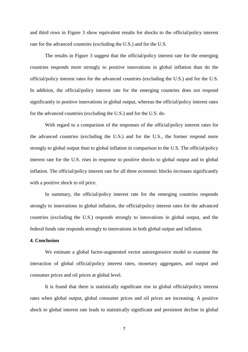
and third rows in Figure 3 show equivalent results for shocks to the official/policy interest

rate for the advanced countries (excluding the U.S.) and for the U.S.

The results in Figure 3 suggest that the official/policy interest rate for the emerging

countries responds more strongly to positive innovations in global inflation than do the

official/policy interest rates for the advanced countries (excluding the U.S.) and for the U.S.

In addition, the official/policy interest rate for the emerging countries does not respond

significantly to positive innovations in global output, whereas the official/policy interest rates

for the advanced countries (excluding the U.S.) and for the U.S. do.

With regard to a comparison of the responses of the official/policy interest rates for

the advanced countries (excluding the U.S.) and for the U.S., the former respond more

strongly to global output than to global inflation in comparison to the U.S. The official/policy

interest rate for the U.S. rises in response to positive shocks to global output and to global

inflation. The official/policy interest rate for all three economic blocks increases significantly

with a positive shock to oil price.

In summary, the official/policy interest rate for the emerging countries responds

strongly to innovations in global inflation, the official/policy interest rates for the advanced

countries (excluding the U.S.) responds strongly to innovations in global output, and the

federal funds rate responds strongly to innovations in both global output and inflation.

4. Conclusion

We estimate a global factor-augmented vector autoregressive model to examine the

interaction of global official/policy interest rates, monetary aggregates, and output and

consumer prices and oil prices at global level.

It is found that there is statistically significant rise in global official/policy interest

rates when global output, global consumer prices and oil prices are increasing. A positive

shock to global interest rate leads to statistically significant and persistent decline in global

8

M2, reduced CPI and nominal oil price, and to reduced global output. Global liquidity, global

output, global prices and oil price explain statistically significant fractions of forecast error

variance decomposition in the principal component for global official/policy interest rates, in

amounts given by 21%, 15%, 8% and 18%, respectively.

Differences are observed for official/policy interest rates for advanced countries and

emerging countries. The response in official/policy interest rate for the emerging countries is

more to global inflation, for the advanced countries (excluding the U.S.) is more to global

output, and for the U.S. is to both global output and inflation.

Findings suggest that when considering movement in the global level of

official/policy interest rate it is necessary to consider the influence of global variables that

reflect developments in the major developing and developed countries.

References

Bernanke, B., Boivin, J., Eliasz, P.S., 2005. Measuring the Effects of Monetary Policy: A

Factor-augmented Vector Autoregressive (FAVAR) Approach. Quarterly Journal of

Economics 120, 387-422.

Barro, R.J., Sala-i-Martin, X., 1990. World Real Interest Rates. National Bureau of Economic

Research NBER Macroeconomics Annual 5, 15-74.

Grossman, V., Marinez-Garcia. E., and Mack., A., 2013. Database of Global Economic

Indicators (DGEI): A Methodological Note. Federal Reserve Bank of Dallas, Globalization

and Monetary Policy Institute. Working Paper No. 166.

Koop, G., Pesaran, M.H., Potter, S.M., 1996. Impulse response analysis in nonlinear

multivariate models. Journal of Econometrics 74, 119–147.

Pesaran, M.H., Shin, Y., 1998. Generalized Impulse Response Analysis in Linear

Multivariate Models. Economics Letters 58, 17–29.

Stock, J., Watson, M., 2005. Macroeconomic Forecasting Using Diffusion Indexes. Journal

of Business and Economic Statistics 20, 147–62.

Thornton, D.L., 2014. Monetary policy: Why money matters (and interest rates don't).

Journal of Macroeconomics 40, 202-213.

9

Table 1: Variance decomposition of Global policy interest rates.

Where *,**,*** indicate coefficients are statistically significant at 10, 5 and 1% level.

Figure 1. Global Official/Policy interest rate. M1:2003 to M12 2013

Months/

Variables

Global

central banks

interest rates

Global

monetary

aggregates

Global CPI Global

outputs

Oil prices

3 95.25*** 0.90 0.98 1.82 1.05

6 69.80*** 9.98 2.58 8.09* 9.55

12 58.35*** 12.88* 6.14 12.05* 10.58*

24 45.68** 18.73* 7.93* 14.10* 13.56**

36 40.38** 20.52* 8.26* 14.52* 16.32**

48 38.25** 20.69* 8.28* 14.58** 18.20**

10

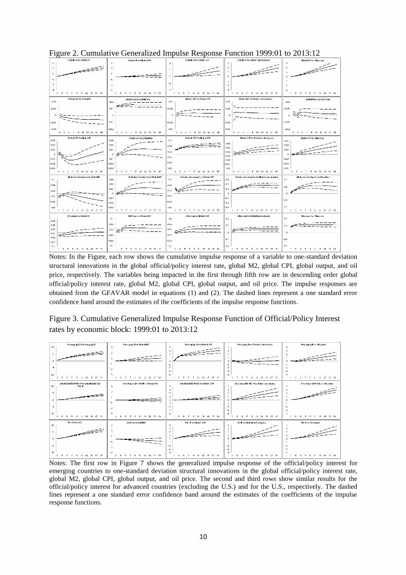
Figure 2. Cumulative Generalized Impulse Response Function 1999:01 to 2013:12

Notes: In the Figure, each row shows the cumulative impulse response of a variable to one-standard deviation

structural innovations in the global official/policy interest rate, global M2, global CPI, global output, and oil

price, respectively. The variables being impacted in the first through fifth row are in descending order global

official/policy interest rate, global M2, global CPI, global output, and oil price. The impulse responses are

obtained from the GFAVAR model in equations (1) and (2). The dashed lines represent a one standard error

confidence band around the estimates of the coefficients of the impulse response functions.

Figure 3. Cumulative Generalized Impulse Response Function of Official/Policy Interest

rates by economic block: 1999:01 to 2013:12

Notes: The first row in Figure 7 shows the generalized impulse response of the official/policy interest for

emerging countries to one-standard deviation structural innovations in the global official/policy interest rate,

global M2, global CPI, global output, and oil price. The second and third rows show similar results for the

official/policy interest for advanced countries (excluding the U.S.) and for the U.S., respectively. The dashed

lines represent a one standard error confidence band around the estimates of the coefficients of the impulse

response functions.

 

 

 

TASMANIAN SCHOOL OF BUSINESS AND ECONOMICS WORKING PAPER SERIES

2014-09 VAR Modelling in the Presence of China’s Rise: An Application to the Taiwanese Economy. Mardi Dun-gey, Tugrul Vehbi and Charlton Martin

2014-08 How Many Stocks are Enough for Diversifying Canadian Institutional Portfolios? Vitali Alexeev and Fran-cis Tapon

2014-07 Forecasting with EC-VARMA Models, George Athanasopoulos, Don Poskitt, Farshid Vahid, Wenying Yao

2014-06 Canadian Monetary Policy Analysis using a Structural VARMA Model, Mala Raghavan, George Athana-sopoulos, Param Silvapulle

2014-05 The sectorial impact of commodity price shocks in Australia, S. Knop and Joaquin Vespignani

2014-04 Should ASEAN-5 monetary policymakers act pre-emptively against stock market bubbles? Mala Raghavan and Mardi Dungey

2014-03 Mortgage Choice Determinants: The Role of Risk and Bank Regulation, Mardi Dungey, Firmin Doko Tchatoka, Graeme Wells, Maria B. Yanotti

2014-02 Concurrent momentum and contrarian strategies in the Australian stock market, Minh Phuong Doan, Vi-tali Alexeev, Robert Brooks

2014-01 A Review of the Australian Mortgage Market, Maria B. Yanotti

2014-10 Contagion and Banking Crisis - International Evidence for 2007-2009 , Mardi Dungey and Dinesh Gaju-rel

2014-11 The impact of post‐IPO changes in corporate governance mechanisms on firm performance: evidence from young Australian firms, Biplob Chowdhury, Mardi Dungey and Thu Phuong Pham

2014-12 Identifying Periods of Financial Stress in Asian Currencies: The Role of High Frequency Financial Market Data, Mardi Dungey, Marius Matei and Sirimon Treepongkaruna

2014-13 OPEC and non‐OPEC oil production and the global economy, Ronald Ratti and Joaquin Vespignani

2014-14 VAR(MA), What is it Good For? More Bad News for Reduced‐form Estimation and Inference, Wenying Yao, Timothy Kam and Farshid Vahid