What Does an Aberrated Photo Tell Us About the Lens and the Scene?

Huixuan Tang Kiriakos N. KutulakosDepartment of Computer Science

University of Toronto{hxtang,kyros}@cs.toronto.edu

Abstract

We investigate the feasibility of recovering lens proper-ties, scene appearance and depth from a single photo con-taining optical aberrations and defocus blur. Starting fromthe ray intersection function of a rotationally-symmetriccompound lens and the theory of Seidel aberrations, we ob-tain three basic results. First, we derive a model for the lensPSF that (1) accounts for defocus and primary Seidel aber-rations and (2) describes how light rays are bent by the lens.Second, we show that the problem of inferring depth andaberration coefficients from the blur kernel of just one pixelhas three degrees of freedom in general. As such it cannotbe solved unambiguously. Third, we show that these de-grees of freedom can be eliminated by inferring scaled aber-ration coefficients and depth from the blur kernel at multi-ple pixels in a single photo (at least three). These theoret-ical results suggest that single-photo aberration estimationand depth recoverymay indeed be possible, given the recentprogress on blur kernel estimation and blind deconvolution.

1. Introduction

Optical aberrations—the blur from imperfect optics—are a fundamental source of image degradation in photog-raphy. Although the task of correcting them has tradition-ally fallen to the lens designer and done with optics [23],correction by computational means is emerging as a power-ful new alternative. Already, computational correction hasbeen included in imaging chains to simplify lens design [5]or to enhance performance [20], and generic photo deblur-ring has been adapted to correct aberrations in restricted set-tings (e.g., for in-focus subjects [11]; scenes with no signif-icant depth variation [21, 22]; photos with only coma [9] oronly axial chromatic aberrations and defocus [6]).Aberrations, however, are not merely a defect to be cor-

rected. The blur they produce depends exclusively on objectdistance and the lens, and thus it conveys potentially valu-able information about both. This leads to a basic question:what information about the lens and the scene can we ex-tract from a single aberrated photo? Answering this ques-tion would give a better understanding of the mutual con-

straints between the aberrated photo, the lens and the scene;taking such constraints into account could lead to better de-blurring algorithms as well.

The nature of aberration-induced blur has made thisquestion difficult to answer. Aberration blur generallyvaries over the field of view, it interacts with defocus tobecome a complex function of depth, and it is affected bya host of imaging parameters—aperture size, focus settingand focal length—in addition to the lens itself. Indeed, acomplete answer to this question is not known even in thebest-possible case where we have perfect information aboutblur, i.e., when the true blur kernel is known at every pixel.

In this paper we make an initial attempt to answer thisquestion for rotationally-symmetric compound lenses ex-hibiting primary Seidel aberrations [15]. We restrict our at-tention to the domain of wide-aperture lenses and geometricoptics, where the effects of diffraction can be ignored (i.e.,the Airy disk is less than one pixel).

Starting from the theory of Seidel aberrations, we derivea general expression for the ray intersection function of alens. This function (1) describes the sensor-side light fielddue to a specific 3D point in the scene, (2) determines itsblurred 2D image on the sensor plane up to vignetting, and(3) depends on nine basic parameters: the coordinates ofthe scene point, the five Seidel aberration coefficients of thelens, and the radius of its exit pupil.

With this forward model at hand we turn to the feasibil-ity of inverting it. We formulate the problem of one-sourceself-calibration, whose goal is to infer the parameters ofthe lens and the coordinates of a point source from itsblurred image on the sensor plane (also known as the blurkernel). By studying the equivalence class of solutionsto this problem we arrive at three basic results. First andforemost, we show that this equivalence class has threedegrees of freedom. Thus, despite the extreme locality ofits input, one-source self-calibration can tell us a great dealabout the lens and the source (the unknown parameters arereduced from nine to just three) but does not determinethem unambiguously. Second, we show that we cannotrecover the pupil radius of the lens but we can eliminateit from the unknowns, reducing the total unknown lensand source parameters to just two. Third, we prove that

we can eliminate the remaining degrees of freedom byviewing a general 3D scene and solving a multi-sourceself-calibration problem. The goal of this problem is toinfer lens parameters and 3D shape by considering manyscene points at once, each corresponding to a differentposition on the sensor plane and possibly a differentdepth. This leads to the main conclusion of our work: intheory, one aberrated photo contains enough informationto reconstruct a scene in 3D and to compute aberrationcoefficients up to a pupil-dependent scale factor.

Related Work Aberrations correspond to distortionsof the optical wavefront and their measurement has beena subject of optics research for decades. Three lines ofwork are particularly relevant here. Techniques based onHartmann-Shack wavefront sensing use the equivalent ofa light-field camera placed directly at the exit pupil of thelens [3,14]. Aberrations are then measured by acquiring thelight field from a point source and comparing it to a known,aberration-free reference light field. More recently, Nalettoet al. [16] showed how aberrations can be estimated with-out direct wavefront sensing. Their idea was to estimateaberrations iteratively using an adaptive optics system thatestimates, compensates, and re-images a point source untilconvergence. Although we rely on the much same underly-ing theory, neither direct measurement of wavefront distor-tions nor adaptive optics are viable options when our onlyinput is a photo captured beyond our control. Last but notleast, Ng et al. [17] propose capturing the sensor-side lightfield using a light field camera and correcting aberrationsby “reshuffling” the captured rays. They not consider theproblem of inferring shape or lens parameters, as we do.Our work is fundamentally about modeling and ana-

lyzing lens blur from very limited image data. As such,it is closely related to computer vision research on PSFestimation [9–11, 21, 22, 24], shape-from-focus and defo-cus [8,18], image deblurring [4,12,13] and camera calibra-tion [1, 2, 27, 28]. These approaches are concerned eitherwith empirical blur modeling and correction, or with scenereconstruction under aberration-free conditions. In contrast,our work here is specifically aimed at aberration analysis, itis purely theoretical, and applies to any algorithmic imple-mentation.A key distinguishing feature of our approach is that it

advocates modeling blur formation rather than the blur it-self: while the blur kernel of a general compound photo-graphic lens may be very hard to model because of its com-plex shape and spatial variation in three dimensions, mod-eling the underlying cause of this complexity—the imper-fect ray deflections—is much easier, involves elementaryaberration optics, and affords a very compact representa-tion. In this respect, our work is similar in spirit to that ofDing et al. [7], where blur formation is studied for catadiop-tric imaging systems with idealized aberration-free lenses.

In the case of an aberrated lens, the potential advantages ofthis approach include (1) improved resistance to over-fittingwhen estimating blur kernels from photos, (2) physical va-lidity of recovered blur kernels and lens parameters, (3) thepotential to infer depth as well as to deblur, (4) the poten-tial to predict the response of the lens to depths other thanthose observed in a photo, and (5) an analysis that is in-dependent of algorithmic implementations. On the otherhand, the price we pay for modeling blur formation is thatthe kernel can no longer be expressed analytically and mustbe computed by numerical integration.

2. Aberrated Image Formation

In an ideal thin lens, all rays from a point in the scene willconverge to a point of perfect focus on the other side of thelens. When aberrations are present, however, rays exitingthe lens may not have their ideal orientation. We begin bydeveloping a physically-based geometric model that explic-itly describes how an aberrated rotationally-symmetric lensbends these rays. Themodel covers both single-element andmulti-element lenses.The basic geometry of our model is shown in Figure 1.

We treat the lens as a black box that transforms the bundleof outgoing rays from a scene point into a new set ofrays that pass through the exit pupil of the lens. Thistransformation can be described in terms of three basicrays: the chief ray that passes through the scene point andthe pupil’s center; an ideal off-axis ray that describes howa thin lens bends the ray at a general point (x, y, 0) onthe exit pupil; and the aberrated off-axis ray that passesthrough the same point on the pupil but deviates from theideal ray.

The ray intersection function Every 3D ray is uniquelydetermined by its intersection with two parallel planes. Wecan therefore fully specify the aberrated ray through point(x, y, 0) by modeling the ray’s intersection, a, with the sen-sor plane.1 Expressing this intersection in terms of thesensor-plane intersections of the chief ray and the ideal off-axis ray we get

a = c︸︷︷︸perspectiveprojection

+ (i− c)︸ ︷︷ ︸displacementdue to defocus

+ v︸︷︷︸displacementdue to aberrations

. (1)

Intuitively, the first term in Eq. (1) can be thought of asthe image of the scene point created by an infinitesimal pin-hole at the pupil’s center. The second term describes theunderlying cause of defocus blur for thin lenses with finite-sized pupils: instead of converging at point c, light raysthrough the pupil will be displaced, depositing irradiance

1We use tilde (˜) to denote quantities on the pupil plane, no markingsfor quantities on the sensor plane, and hat (ˆ) for the in-focus plane. Upper-case symbols denote lens- or scene-specific constants.

exit pupil plane(z = 0)

x

z

pupil point(x, y, 0)

(0, 0, 0)

c

ci

a

in-focus plane(z = f)

sensor plane(z = f)

chief ray

v

scene point(X, 0,−Z)

idealoff-axis ray

aberratedoff-axis ray

Figure 1: Viewing geometry. A scene point is at a distance Z away fromthe exit pupil of an aberrated, rotationally-symmetric lens with focal lengthF . The distance of the ideal in-focus plane from the exit pupil is given bythe thin-lens law: f = F

Z−FZ . We assume throughout this paper that

the sensor plane is at a fixed but unknown distance from the pupil plane.Note that this plane will generally not coincide with the in-focus plane andthus the scene point may be out of focus, as in this figure. By conventionwe take the axis of symmetry of the lens to be the z-axis of the cameracoordinate system. In this coordinate system, we can assume without lossof generality that scene points always lie on the xz-plane.

away from the scene point’s perspective projection. Usingthe notation of Figure 1, from similar triangles we have

i− c =

(f − f

f

)· (x, y) def

= D · (x, y) , (2)

where the constant D represents the “defocus level” of thescene point and can be thought of as a proxy for depth.

Seidel aberrations The third—and most important—termof Eq. (1) captures the effect of aberrations. This termis highly constrained for rotationally-symmetric lenses be-cause the optical wavefront produced by a symmetric lensmust itself be rotationally symmetric. The primary, orSeidel, aberrations arise by expressing this wavefront as arotationally-symmetric polynomial and considering termsup to third order. The details are beyond the scope of thispaper and we refer the reader to [15,26] for the basic theory.The important points are that (1) the aberration-induced dis-placements can be expressed as a linear combination of fiveSeidel displacement fields, (2) the coefficients of this linearcombination depend on exactly five lens-specific aberrationparameters regardless of the number or arrangement of in-ternal lens elements, and (3) when the sensor-plane-to-pupildistance is fixed, the linear combination coefficients can beexpressed as cubic polynomials of the defocus level.More specifically, we show in Appendix A that the dis-

placement vector v is given by the sum

v(x, y, c, D,Σ1, . . . ,Σ5) =

5∑k=1

vk(D,Σ1, . . . ,Σ5) vk(x, y, c) , (3)

Spherical (v1) Coma (v2) Astigmatism (v3) Field curvature (v4)[x2 + y2](x, y) ‖c‖(3x2 + y2, 2xy) ‖c‖2(x, 0) ‖c‖2(x, y)

x

y

O x

y

O x

y

O x

y

O

Figure 2: The Seidel displacement fields. We can visualize the 2D dis-placements caused by aberrations by treating them as vector-valued func-tions of the pupil point (x, y, 0). Four of the resulting vector fields areshown above, along with their analytic expressions (‖.‖ denotes vectornorm). Please zoom into the electronic copy to see details. The fifth vectorfield—field distortion—is v5(x, y, c) = ‖c‖2c. This field is not shownbecause it is independent of x and y and would appear as a field of identicalvectors.

whereD is the defocus level; the Seidel displacement fieldsvk() and coefficient functions vk() are defined in Figure 2and Table 1, respectively; and Σ1, . . . ,Σ5 are lens-specificparameters that control the contribution of individual Seidelaberrations in Table 1.

Equation (3) tells us that just five parametersΣ1, . . . ,Σ5

are enough to characterize the aberrated behavior of ageneral rotationally-symmetric lens up to third order: oncethese parameters are known, we can determine how theaberrated lens redirects ideal off-axis rays from any givenpoint in the scene.

The PSF Integral Equations (1)-(3) lead to a parametricmodel for the lens point-spread function (PSF). This modeltreats the PSF as a five-dimensional function that maps 3Dpoints in the scene to their 2D image on the sensor plane.

The image of a specific 3D point is the result of radiancethat is transported through the exit pupil of the lens. To ob-tain an expression for this kernel, we restrict our attentionto cases where scattering and reflection inside the lens [19]are negligible and where the pupil-to-scene distance is largecompared to the radius of the pupil itself. In this case,the radiance transported along all aberrated rays is approx-imately the same. This turns the PSF into a “ray-countingintegral” that measures the distribution of aberrated-ray in-tersections with the sensor plane.

In particular, given a scene point with perspective pro-jection c and defocus levelD, the irradiance at a point q onthe sensor plane is an integral over the exit pupil:

Spherical v1(D,Σ1, . . . ,Σ5) = Σ1+Σ2D+Σ3D2+Σ4D2+Σ5D3

Coma v2(D,Σ1, . . . ,Σ5) = Σ2+2Σ3D+2Σ4D+3Σ5D2

Astigmatism v3(D,Σ1, . . . ,Σ5) = Σ3+2Σ5DF. curvature v4(D,Σ1, . . . ,Σ5) = Σ4+Σ5DF. distortion v5(D,Σ1, . . . ,Σ5) = Σ5

Table 1: Coefficient functions of the Seidel displacement fields. Theconstants Σ1, . . . ,Σ5 are the five Seidel aberration parameters of the lens.

PSFR,Σ1,...,Σ5(c, D,q) = β1(c) ·∫

‖(x,y)‖≤Rδ(∥∥q− a(x, y, c, D,Σ1, . . . ,Σ5)

∥∥)β2(x, y, c) dxdy (4)

where R is the radius of the exit pupil; Σ1, . . . ,Σ5 are theparameters controlling the five Seidel aberrations; a() is thesensor-plane intersection of the aberrated ray through point(x, y, 0) on the exit pupil (Eqs. (1)-(3)); δ() is Dirac’s delta,used to “test” if the aberrated ray passes through point qon the sensor plane; β1(c) converts radiance to irradianceand models vignetting due to the cos4-falloff of obliquechief rays2; and β2(x, y, c) is a binary function that mod-els vignetting due to ray occlusion, i.e., it is zero if lightis blocked by internal lens components before reaching theexit pupil.3

The PSF defined by Eq. (4) cannot be expressed in a sim-ple analytic form even for relatively simple types of opticalaberration. Therefore, we forgo analytical approximationsof the PSF—which can introduce considerable error—andfocus instead on representing the ray intersection functionanalytically.

3. Analysis of One-Source Self-Calibration

The PSF integral in Eq. (4) can be thought of as a for-ward model for local image formation: if we know the 3Dcoordinates of an isolated point light source and know allthe camera parameters (sensor-to-pupil distance, pupil ra-dius, lens focal length, vignetting functions and aberrationparameters), we can compute the source’s 2D image on thesensor plane, i.e., its blur kernel. We now turn to the as-sociated local inverse problem: given the blur kernel of anisolated 3D source, what can we infer about the source’s 3Dcoordinates and about the lens?Computing the blur kernel from a single photo—also

known as blind image deblurring—is itself a very diffi-cult inverse problem because aberrations, scene occlusionsand depth variations cause the blur kernel to vary spa-tially [10, 11]. Here we sidestep this difficulty by seekingto establish the limits of local inference: we ask what canbe inferred about the lens and about an isolated point in thebest-case scenario, when our deblurring algorithm has re-covered the exact blur kernel at the point’s projection andthere are no occlusions or depth discontinuities. In partic-ular, we show that even under this idealized scenario sig-nificant ambiguities still exist, preventing us from recover-ing depth and aberration parameters unambiguously. Thus,all we can hope to achieve from such a local analysis is to

2This falloff reduces the apparent brightness of scene points that projectnear image corners [2, 28].

3This function “crops” the PSF to a region that is always an intersectionof disks for rotationally-symmetric lenses [15].

(X, 0,−Z)

(Rx,Ry, 0)

a

c

R

sensor plane(z = f)

x

z

aberratedoff-axis ray

(a) True solution T

(X′, 0,−Z′)

(R′x, R′y, 0)

a

c′

R′

sensor plane(z = f)

x

z

aberratedoff-axis ray

(b)Blur-consistent solution T ′

Figure 3: Blur consistency. (a) Source (X, 0,−Z) is viewed by the“true” lens. (b) A second source on the xz-plane is viewed by a lens with adifferent pupil radius and different aberration parameters. For the solutionin (b) to be blur consistent, every aberrated off-axis ray must intersect thesensor plane at the same point a that the corresponding aberrated ray in (a)does.

constrain these unknowns to a low-parameter family of so-lutions that are consistent with the observed blur kernel.Consider a point source whose perspective projection on

the sensor plane is c, its depth is Z and its defocus level isD. According to Eq. (4), the source’s image on the sensorplane depends on depth only indirectly via the defocus level.Since the relation between defocus and depth involves theunknown sensor-to-pupil distance (Eq. (2)) as well as theunknown focal length of the lens (Figure 1), we cannot in-fer the source’s depth solely from the blur kernel at c. Wetherefore concentrate on inferring the defocus level D aswell as the aberration parameters of the lens.4

To quantify the ambiguities of this inference problemwe introduce a notion of blur consistency between its so-lutions. Specifically, let T = 〈c, D,R,Σ1, . . . ,Σ5〉 bea tuple containing the source’s “true” perspective projec-tion and defocus level as well as the true pupil radiusand lens aberration parameters. We call a tuple T ′ =〈c′, D′, R′,Σ′

1, . . . ,Σ′5〉, corresponding to another solution,

blur consistent to T if it redirects rays toward the sensorplane in exactly the same way that T does (Figure 3):

Definition 1 (Blur-consistent solution). T ′ and T are blurconsistent if their ray intersection functions agree on a sub-set of their pupil after accounting for differences in pupilradius:

a(R′x, R′y, c′, D′, Σ′1, . . . ,Σ

′5) =

a(Rx, Ry, c, D, Σ1, . . . ,Σ5)

for all (x, y) in an open subset of the unit circle. (6)

Intuitively, blur consistency is both weak and strong asa constraint. It is weak because it is very local: the lens

4Note that the inference of D is trivial for an ideal thin lens: the blurkernel in that case is a uniform disk whose radius is equal to DR, whereR is the unknown radius of the exit pupil. Thus the blur kernel determinesthe defocus level up to the unknown global scale factor R. When the lensis aberrated, as we assume here, the relation between the blur kernel andthe defocus level is far more complex.

⎡⎢⎢⎢⎣

0 0 0 0 ‖c′‖30 0 0 ‖c′‖2 D′‖c′‖20 0 ‖c′‖2 ‖c′‖2 3D′‖c′‖20 ‖c′‖ 2D′‖c′‖ 2D′‖c′‖ 3(D′)2‖c′‖1 D′ (D′)2 (D′)2 (D′)3

⎤⎥⎥⎥⎦

⎡⎢⎢⎢⎣

Σ′1

Σ′2

Σ′3

Σ′4

Σ′5

⎤⎥⎥⎥⎦ =

⎡⎢⎢⎢⎣

0 0 0 0 ‖c‖30 0 0 ‖c‖2 D‖c‖20 0 ‖c‖2 ‖c‖2 3D‖c‖20 ‖c‖ 2D‖c‖ 2D‖c‖ 3D2‖c‖1 D D2 D2 D3

⎤⎥⎥⎥⎦

⎡⎢⎢⎢⎣

Σ1

Σ2

Σ3

Σ4

Σ5

⎤⎥⎥⎥⎦+

⎡⎢⎢⎢⎣

‖c‖ − ‖c′‖D −D′D −D′

00

⎤⎥⎥⎥⎦ (9)

defined by T ′ need not reproduce a set of ray-sensor planeintersections that is identical to T ’s for all possible pointsources; there simply needs to be some source (with per-spective projection c′ and defocus level D′) that results inthe same bundle of rays as those produced by the true sourceand the true lens. On the other hand, blur consistency isstrong because it does not merely require that the two lensesbend isolated rays in a similar fashion—it requires that adense subset of rays exiting their pupils behave exactly thesame way. The advantage of this definition is that it al-lows us to reduce our analysis to the study of ambiguities ofthe ray intersection function. This function has a relativelysimple analytical form (Eqs. (1)-(3)) and does not dependon lens vignetting.5

While it might seem that blur consistency is too stronga constraint to leave much room for ambiguities, this is notthe case. In particular, we prove that shape and lens param-eters can only be known up to an unresolvable three-degree-of-freedom ambiguity:

Theorem 1 (Space of blur-consistent solutions). The blurconsistent solutions T ′ span a three-parameter family in-dexed by the pupil radius R′, the defocus level D′ and thedistance ‖c′‖ of the scene point’s perspective projectionfrom the optical axis.

Theorem 1 follows from two lemmas which make theseambiguities explicit. Lemma 1 below identifies a generalscale ambiguity; this ambiguity allows us to change the sizeof the exit pupil from R to R′ while simultaneously rescal-ing the defocus level and the aberration parameters:

Lemma 1 (Pupil radius ambiguity). The tuple

〈c, D R

R′ , R′, Σ1

(R

R′

)3

, Σ2

(R

R′

)2

, Σ3R

R′ , Σ4R

R′ , Σ5〉 (7)

is blur consistent to T for any R′ > 0.

Since the pupil radius is a completely free parameter, be-low we keep its value fixed to R for simplicity.Lemma 2 now tells us that we can treat the source’s un-

known defocus level and perspective projection on the xz-plane as free parameters. As long as this projection is not atthe origin, we can achieve blur consistency by assigning anyvalue to D′ and ‖c′‖. To ensure consistency the aberrationparameters must then satisfy a system of linear equations.

5By requiring agreement on a dense subset of the pupil rather than thefull pupil, blur consistency is not affected by vignetting either.

Lemma 2 (Projection and defocus ambiguities). The tuple

〈c′, D′, R, Σ′1, Σ

′2, Σ

′3, Σ

′4, Σ

′5〉 (8)

is blur consistent to T if and only if (1) c′ is on the xz-plane and (2) the aberration parameters Σ′

1, . . . ,Σ′5 satisfy

the 5× 5 linear system in Eq. (9).

Proof sketch of Lemmas 1 and 2. We first obtain an expression forthe ray intersection function by combining Eqs. (1)-(3) with theexpressions in Figure 2, grouping terms with identical 2D dis-placement vectors, and expressing pupil coordinates as multiplesof the pupil radius R:

a(Rx, Ry, c,D,Σ1, . . . ,Σ5) =(1 + v5‖c‖2

)︸ ︷︷ ︸

perspective+ field distortion

c +

(D + v4‖c‖2︸ ︷︷ ︸

defocus+ field curvature

+ v1R2[x2 + y2]

)︸ ︷︷ ︸

spherical

(Rx,Ry)

+ v2‖c‖︸ ︷︷ ︸coma

(R2x2 +R2 y2, 2R2xy) + v3‖c‖2︸ ︷︷ ︸astigmatism

(Rx, 0) . (10)

We then substitute into Eq. (10) the expressions for vk fromTable 1 to get a new expression for the ray intersection functionthat is exclusively in terms of x, y, c, D,R and Σ1, . . . ,Σ5. Thisexpression is a polynomial in x and y involving all the monomialsup to third order:

{1, x, y, xy, x2, y2, x2y, xy2, x3, y3} . (11)

The coefficients of these monomials depend on c, D, R andΣ1, . . . ,Σ5. Moreover, because the expressions in Table 1 arelinear in Σ1, . . . ,Σ5, the monomial coefficients are linear in allfive aberration parameters. Lemma 1 now follows by showing thatthe variable substitution implied by Eq. (7) does not alter the co-efficients of these monomials because R′ cancels out.To prove Lemma 2, we combine Eq. (6) and the polynomial

expression for the ray intersection function to obtain an equalitybetween two polynomials of x and y, one whose coefficients de-pend on c, D, R,Σ1, . . . ,Σ5 and one whose coefficients dependon c′, D′, R,Σ′

1, . . . ,Σ′5. We then observe that since equality be-

tween these polynomials must hold for all x, y in an open set,the coefficients of all monomials listed in Eq. (11) must be thesame. This gives rise to six distinct equations that are linear inΣ1, . . . ,Σ5,Σ

′1, . . . ,Σ

′5 and also involve c, c

′ and D,D′. One ofthese equations—corresponding to the constant monomial—is sat-isfied only when c′ is a multiple of c. This leads to the first condi-tion of Lemma 2. The other five equations are linear inΣ′

1, . . . ,Σ′5

and give rise to the system in Eq. (9). Note that the coefficient ma-trix at the left-hand side of the equation is invertible if and only if‖c′‖ �= 0.

4. Multi-Source Self-Calibration

A natural question is whether the ambiguities in one-source self-calibration can be eliminated by consideringmore than one source. Here we show that in general theanswer is yes: blur consistency with three sources at pos-sibly different depths is enough to reduce the unknowns tojust the pupil radiusR. This means that the lens parametersand the defocus level of multiple sources can be recoveredfrom a single photo, up to a global scale ambiguity due tothe pupil radius.To make this concrete, let c1, . . . , cK be the true per-

spective projection of K sources with ‖ci‖ �= ‖cj‖,and let D1, . . . , DK be their true defocus levels. Sinceall sources are imaged by the same lens, the true solu-tion of the corresponding one-source self-calibration prob-lems will be Tk = 〈ck, Dk, R,Σ1, . . . ,Σ5〉 for k =1, . . . ,K . Now let Σ′

1, . . . ,Σ′5 be another set of aberra-

tion parameters that yields blur-consistent solutions T ′k =

〈c′k, D′k, R,Σ′

1, . . . ,Σ′5〉 for all k = 1, . . . ,K .

Theorem 2 (Multi-source self-calibration). Generically,the space of solutions that are blur consistent to K sourcesis discrete forK > 2.

Proof sketch. Let T ′1 = 〈c′1, D′

1, R,Σ′1, . . . ,Σ

′5〉 be a blur-

consistent solution for the first source. Applying Eq. (9) to thissolution and performing the matrix-vector product yields a systemof five third-order polynomial equations in the seven unknowns‖c′1‖, D′

1,Σ′1, . . . ,Σ

′5. Each of these five equations introduces at

least one new variable into the system: considering the matrix inthe left-hand side of Eq. (9) row by row, the equations introduce‖c′1‖ andΣ′

5; Σ′4 andD

′1; Σ

′3; Σ

′2; and Σ

′1, respectively. It follows

that these equations are algebraically independent [25].Now let T ′

2 = 〈c′2, D′2, R,Σ′

1, . . . ,Σ′5〉 be a blur-consistent

solution for the second source. Applying Eq. (9) to this solutionyields an additional five polynomial equations and two extra un-knowns, namely c′′2 andD

′′2 . We now consider the number of inde-

pendent constraints introduced by the addition of this new source,i.e., the number of algebraically-independent equations in the en-larged system. Specifically, we focus on the following three equa-tions from the system:

Σ′5‖c′2‖3 + ‖c′2‖ = α (12)

Σ′4‖c′2‖2 +Σ′

5D′2‖c′2‖2 +D′

2 = β (13)

Σ′1 + Σ′

2D′2 + Σ′

3D′22+Σ′

4D′22+ Σ′

5D′23= γ (14)

where α, β, γ are constants specific to the true lens and the truesecond source. Solving for ‖c′2‖2 in Eq. (13), squaring both sidesof Eq. (12) and combining the result we get an equation that de-pends only on one unknown, D′

2, that is specific to the secondsource:

(β −D′2)

3(Σ′5)

2 + 2(β −D′2)

2(Σ′4 + Σ′

5D′2)(Σ

′5)+

(β −D′2)(Σ

′4 + Σ′

5D′2)

2 − α2(Σ′4 + Σ′

5D′2)

3 = 0 . (15)

The highest-order monomial in D′2 is cubic in both Eqs. (14)

and (15) and its coefficient is Σ′5 and −4Σ′

52 − βΣ′

53, respec-

tively. Generically, these coefficients are distinct and cannot becancelled by any polynomial combination of the two equations.6

It follows that Eqs. (12)-(14) are algebraically independent.Therefore, the addition of a second source adds two un-

knowns but three independent equations. The addition of the thirdsource leads to a system with 11 unknowns and 11 algebraically-independent equations.

5. Discussion

We now interpret the theoretical results of Sections 3and 4 from a more practical perspective, in the context ofthree tasks:

• Blind local PSF estimation: estimate the 2D blur ker-nel at a pixel p in an aberrated photo.

• Non-blind lens calibration and PSF prediction: giventhe blur kernel and defocus level at one or more pixels,estimate the lens aberration parameters and predict the2D blur kernel for other pixels, defocus levels, pupilsizes, focus settings and focal lengths.

• Blind lens self-calibration and scene reconstruction:given a photo of an unknown scene with depth vari-ations, estimate the aberration parameters of the lensand the defocus level at each pixel.

A consequence of Lemma 1 that applies to all three tasksis that the radius of the exit pupil does not constrain the rayintersection function or the blur kernel. Therefore we canassume R = 1 without compromising our ability to modelblur accurately. Defocus levels and aberration parametersare recoverable up to an unknown scale factor (Eq. (7)).

Blind local deblurring In typical blind deblurring, thegoal is to estimate the “hidden” deblurred photo as wellas the 2D blur kernel. Although specific approaches dif-fer on the choice of image prior and kernel representation(e.g., [13, 22]) they all model the blur kernel directly eitheras an analytical function or using a non-parametric repre-sentation. Lemma 2 suggests an alternative approach: (1)model the kernel indirectly via its ray intersection function,(2) use Eq. (4) to evaluate the blur kernel numerically, and(3) fit it to local image measurements by optimizing overthe five aberration parameters. We can do this for a pixel pby settingR = 1 and ‖c′‖ = ‖p‖ in Eqs. (8) and (4), choos-ing an arbitrary non-zero value for its defocus levelD′, andoptimizing over Σ′

1, . . . ,Σ′5 in a neighbourhood around p.

This optimization should be considered a form of localover-fitting. Specifically, Lemma 2 says that this optimiza-tion is flexible enough to provide a perfect fit under noise-less conditions. The optimized and the true aberration pa-

6Specifically, cancellation can only occur for discrete values of Σ′5,

including Σ′5 = 0.

rameters will not be identical, however, but related by theunknown transformation in Eq. (9). This transformation isvalid only in the neighbourhood of pixel p and thus the op-timized constants will be inconsistent, in general, with theblur kernel elsewhere on the sensor plane.

Non-blind lens self-calibration and PSF prediction Nowsuppose we know the exact blur kernel and defocus levelat K points on a fronto-parallel target (e.g., using the ap-proach of Joshi et al. [10]). To fit the blur kernel of all thesepixels we cannot just choose arbitrary values for their de-focus levels and perspective projections, as in the case ofblind local deblurring; these unknowns must be optimizedas well. In general, this is an optimization over 6 + K un-knowns corresponding to aberration parameters, the target’sdefocus level, and the K per-pixel projections. Theorem 2suggests that this procedure is not ill-posed in general, al-though uniqueness of a solution cannot be guaranteed: thesystem of polynomial equations that is implicitly solved bythis optimization may have numerous solutions, especiallywhen the numberK of pixels participating in the optimiza-tion is small.This optimization procedure should ideally result in a set

of aberration parameters that describe the aberration behav-ior of the lens according to Eq. (4). As such, they can beused to predict the blur kernel for any 3D point in the sceneand any pupil radius, modulo the effects of vignetting anddiffraction. It is important to note, however, that predictionsfor other pupil-to-sensor distances and other focal lengthsare not possible in general for two reasons. First, com-mon photographic lenses contain movable internal elementsthat are adjusted in order to adjust focus or zoom. Sincethese internal motions change the aberration parameters ofthe lens, the coefficients computed for one focus or zoomsetting cannot be used for other settings. Second, aberra-tion parameters in our model are expressed in units specificto the position of the sensor plane. As such, their valuescannot be readily converted to coefficients corresponding toother pupil-to-sensor distances.

Blind lens self-calibration and scene reconstructionTheorem 2 suggests that there are no theoretical barriersto estimating scene structure in addition to aberration pa-rameters from a single photo. In this sense, the problemcan be thought of as unifying the problems of blind imagedeblurring [12, 13], depth-from-defocus [8, 18] and image-based aberration analysis [9–11, 21, 22, 24]. In practice, ofcourse, this problem presents significant challenges becausevignetting and depth discontinuities make the underlyingoptimization problem very challenging.

Vignetting The two forms of vignetting modeled in Eq. (4)impact aberration analysis in very different ways. Vi-gnetting due to oblique chief rays (factor β1(c)) simplyscales the blur kernel without affecting its structure. In prac-

tice, ignoring this term means that we cannot infer the ra-diance due to individual scene points but does not affectour ability to model blur accurately. On the other hand, vi-gnetting due to ray occlusion (term β2(x, y, c)) can affectthe shape of the blur kernel significantly, especially nearimage corners [1, 11, 24]. We believe that taking this formof vignetting into account will be critical to achieve goodimage deblurring and accurate aberration estimation.

6. Self-Calibration Experiments

As an initial validation of our theory, we show experi-ments on non-blind self-calibration and PSF prediction: wefit our PSF formation model to known blur kernels atK pix-els and assess the model’s predictions at other pixels and de-focus levels. A Canon EOS 5DMkII camera and the 135mmF/2.8 “Softfocus” lens were used for all experiments. Thislens is deliberately designed to exhibit prominent sphericalaberrations that alter the conventional lens bokeh.

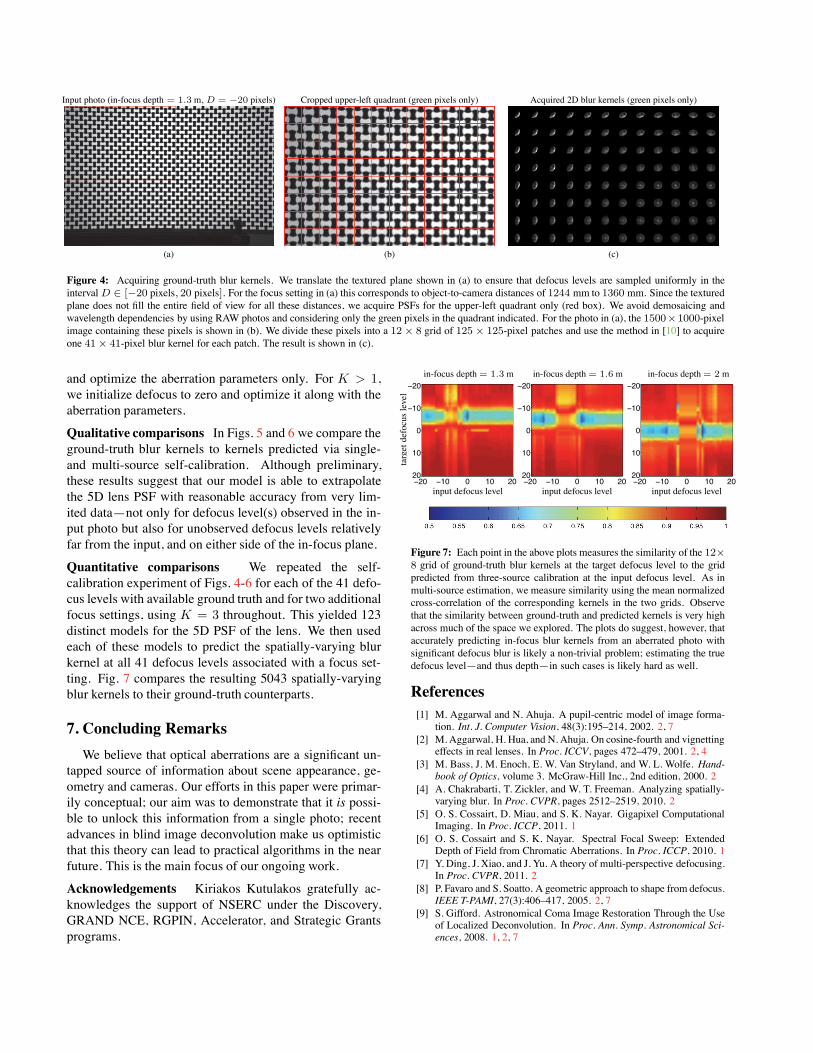
Ground-truth acquisition of 5D PSFs We begin bydensely sampling the 5D lens PSF for a fixed pupil-to-sensor distance f (Fig. 1). This is done by (1) mountinga textured plane onto a linear translation stage that is paral-lel to the optical axis, (2) focusing the lens onto that planeusing the camera’s auto-focus mechanism and (3) movingthe plane to 41 positions without changing the focus set-ting again. We capture two RAW photos at each position:a wide-aperture photo at F/2.8 that provides an aberratedand defocused view of the plane, and a narrow-aperturephoto at F/32 that we use to infer the plane’s sharp im-age. In particular, we register the plane’s known texture tothe narrow-aperture photo and consider the registered tex-ture to be a blur-free image of the plane.7 This image, alongwith the wide-aperture photo, are given as input to Joshiet al.’s non-blind deconvolution method [10]. The result isan estimate of the spatially-varying blur kernel of the wide-aperture photo, which we treat as ground truth (Fig. 4).

Single- and multi-source self-calibration Our self-calibration procedure amounts to fitting the PSF formationmodel of Eq. (4) to the ground-truth 2D blur kernels at Kpixels in a photo. We assume that vignetting due to ray oc-clusion can be ignored (β2(x, y, c) ≈ 1) and fit our modelby maximizing the mean normalized cross-correlation be-tween theK ground-truth and predicted kernels. This mea-sure is unaffected by scaling of the kernels’ intensities andthus accounts for vignetting due to oblique chief rays. Theactual optimization is implemented using L-BFGS and nu-merical gradient computation, with all aberration parame-ters initialized to zero. Since the defocus level is uncon-strained when fitting our model to K = 1 kernels (Theo-rem 1), we set defocus to its ground-truth value in this case

7Note that the narrow-aperture photo may contain diffraction blur andthus cannot be treated as a blur-free image.

Input photo (in-focus depth = 1.3 m, D = −20 pixels) Cropped upper-left quadrant (green pixels only) Acquired 2D blur kernels (green pixels only)

(a) (b) (c)

Figure 4: Acquiring ground-truth blur kernels. We translate the textured plane shown in (a) to ensure that defocus levels are sampled uniformly in theintervalD ∈ [−20 pixels, 20 pixels]. For the focus setting in (a) this corresponds to object-to-camera distances of 1244 mm to 1360 mm. Since the texturedplane does not fill the entire field of view for all these distances, we acquire PSFs for the upper-left quadrant only (red box). We avoid demosaicing andwavelength dependencies by using RAW photos and considering only the green pixels in the quadrant indicated. For the photo in (a), the 1500×1000-pixelimage containing these pixels is shown in (b). We divide these pixels into a 12 × 8 grid of 125 × 125-pixel patches and use the method in [10] to acquireone 41× 41-pixel blur kernel for each patch. The result is shown in (c).

and optimize the aberration parameters only. For K > 1,we initialize defocus to zero and optimize it along with theaberration parameters.

Qualitative comparisons In Figs. 5 and 6 we compare theground-truth blur kernels to kernels predicted via single-and multi-source self-calibration. Although preliminary,these results suggest that our model is able to extrapolatethe 5D lens PSF with reasonable accuracy from very lim-ited data—not only for defocus level(s) observed in the in-put photo but also for unobserved defocus levels relativelyfar from the input, and on either side of the in-focus plane.

Quantitative comparisons We repeated the self-calibration experiment of Figs. 4-6 for each of the 41 defo-cus levels with available ground truth and for two additionalfocus settings, using K = 3 throughout. This yielded 123distinct models for the 5D PSF of the lens. We then usedeach of these models to predict the spatially-varying blurkernel at all 41 defocus levels associated with a focus set-ting. Fig. 7 compares the resulting 5043 spatially-varyingblur kernels to their ground-truth counterparts.

7. Concluding Remarks

We believe that optical aberrations are a significant un-tapped source of information about scene appearance, ge-ometry and cameras. Our efforts in this paper were primar-ily conceptual; our aim was to demonstrate that it is possi-ble to unlock this information from a single photo; recentadvances in blind image deconvolution make us optimisticthat this theory can lead to practical algorithms in the nearfuture. This is the main focus of our ongoing work.

Acknowledgements Kiriakos Kutulakos gratefully ac-knowledges the support of NSERC under the Discovery,GRAND NCE, RGPIN, Accelerator, and Strategic Grantsprograms.

targetdefocuslevel

in-focus depth= 1.3 m in-focus depth= 1.6 m in-focus depth= 2 m

−20 −10 0 10 20

−20

−10

0

10

20−20 −10 0 10 20

−20

−10

0

10

20−20 −10 0 10 20

−20

−10

0

10

20

input defocus level input defocus level input defocus level

Figure 7: Each point in the above plots measures the similarity of the 12×8 grid of ground-truth blur kernels at the target defocus level to the gridpredicted from three-source calibration at the input defocus level. As inmulti-source estimation, we measure similarity using the mean normalizedcross-correlation of the corresponding kernels in the two grids. Observethat the similarity between ground-truth and predicted kernels is very highacross much of the space we explored. The plots do suggest, however, thataccurately predicting in-focus blur kernels from an aberrated photo withsignificant defocus blur is likely a non-trivial problem; estimating the truedefocus level—and thus depth—in such cases is likely hard as well.

References[1] M. Aggarwal and N. Ahuja. A pupil-centric model of image forma-

tion. Int. J. Computer Vision, 48(3):195–214, 2002. 2, 7[2] M. Aggarwal, H. Hua, and N. Ahuja. On cosine-fourth and vignetting

effects in real lenses. In Proc. ICCV, pages 472–479, 2001. 2, 4[3] M. Bass, J. M. Enoch, E. W. Van Stryland, and W. L. Wolfe. Hand-

book of Optics, volume 3. McGraw-Hill Inc., 2nd edition, 2000. 2[4] A. Chakrabarti, T. Zickler, and W. T. Freeman. Analyzing spatially-

varying blur. In Proc. CVPR, pages 2512–2519, 2010. 2[5] O. S. Cossairt, D. Miau, and S. K. Nayar. Gigapixel Computational

Imaging. In Proc. ICCP, 2011. 1[6] O. S. Cossairt and S. K. Nayar. Spectral Focal Sweep: Extended

Depth of Field from Chromatic Aberrations. In Proc. ICCP, 2010. 1[7] Y. Ding, J. Xiao, and J. Yu. A theory of multi-perspective defocusing.

In Proc. CVPR, 2011. 2[8] P. Favaro and S. Soatto. A geometric approach to shape from defocus.

IEEE T-PAMI, 27(3):406–417, 2005. 2, 7[9] S. Gifford. Astronomical Coma Image Restoration Through the Use

of Localized Deconvolution. In Proc. Ann. Symp. Astronomical Sci-ences, 2008. 1, 2, 7

Ground-truth blur kernels Predicted blur kernelsK = 1 K = 3 K = 5 K = 12

D=

−20

D∗

D=

0

D∗+

20

D=

20

D∗+

40

Figure 5: Ground-truth kernels vs. kernels predicted by single- or multi-source self-calibration. In this experiment, we fitted our PSF model to K ofthe ground-truth blur kernels in Fig. 4c. The model was then used to extrapolate the 5D PSF of the lens. Top left: For K = 1 we used only the redkernel; for K = 3 we used the pink kernels as well; for K = 5 we added the green kernels and for K = 12 the yellow kernels were also included.All kernels were chosen at random except for the kernel at the upper-left and the lower-right corner, whose position was fixed. Column 1, top to bottom:Ground-truth blur kernels for three distant defocus levels. Please zoom into the electronic copy to see details. Columns 2-4: To predict the 2D blur kernel atpreviously-unobserved pixels and defocus levels of the textured plane, we first estimated the aberration parameters and the K per-pixel defocus levels. Wethen averaged these levels to estimate the textured plane’s mean defocus level D∗. Observe that our model’s predictions match the ground-truth kernels atD = 0 and D = 20 quite well despite the input photo’s very different defocus level. This suggests that D∗ is fairly accurate in this experiment: indeed,D∗ was estimated to be−20.453,−20.275 and −20.506 pixels forK = 3, 5 and 12, respectively.

DefocusD (pixels)−20 −10 0 10 20

Ground

truth

1

K

35

12

DefocusD (pixels)−20 −10 0 10 20

DefocusD (pixels)−20 −10 0 10 20

(a) (b) (c)

Figure 6: An alternative visualization of the experimental results in Fig. 5. Instead of showing how the ground-truth and predicted blur kernels vary overthe image plane, we show how they vary with defocus—and thus object depth—at three locations on the sensor plane: (a) the red patch in Fig. 5; (b) thepink patch at the bottom-right corner, which lies near the camera’s optical center; and (c) a randomly-selected patch that was not used for PSF model fitting.Observe that both the ground-truth and the predicted kernels are highly asymmetric relative to the in-focus plane. Moreover, despite the very limited dataused for PSF fitting, our model’s predictions appear quite accurate. This accuracy, however, degrades near optical centre (b) where the predicted blur kerneldoes not exhibit the prominent ring-like structure that the ground-truth kernel has forD > 0.

[10] N. Joshi, R. Szeliski, and D. J. Kriegman. PSF estimation using sharpedge prediction. In Proc. CVPR, 2008. 2, 4, 7, 8

[11] E. Kee, S. Paris, S. Chen, and J. Wang. Modeling and RemovingSpatially-Varying Optical Blur. In Proc. ICCP, 2011. 1, 2, 4, 7

[12] D. Krishnan, T. Tay, and R. Fergus. Blind deconvolution using a

normalized sparsity measure. In Proc. CVPR, pages 233–240, 2011.2, 7

[13] A. Levin, Y.Weiss, F. Durand, andW. Freeman. Understanding BlindDeconvolution Algorithms. IEEE T-PAMI, 33(12):2354–2367, 2011.2, 6, 7

[14] J. Liang, B. Grimm, S. Goelz, and J. F. Bille. Objective measurementof wave aberrations of the human eye with the use of a Hartmann-Shack wave-front sensor. JOSA-A, 11(7):1949–1957, 1994. 2

[15] V. Mahajan. Optical Imaging and Aberrations. SPIE, 1998. 1, 3, 4,10

[16] G. Naletto, F. Frassetto, N. Codogno, E. Grisan, S. Bonora,V. Da Deppo, and A. Ruggeri. No wavefront sensor adaptive opticssystem for compensation of primary aberrations by software analysisof a point source image. Appl Optics, 46(25):6427–6433, 2007. 2

[17] R. Ng and P. M. Hanrahan. Digital Correction of Lens Aberrationsin Light Field Photography. In Proc. Int. Optical Design. OpticalSociety of America, 2006. 2

[18] A. P. Pentland. A New Sense for Depth of Field. IEEE T-PAMI,(4):523–531, 1987. 2, 7

[19] R. Raskar, A. Agrawal, C. Wilson, and A. Veeraraghavan. GlareAware Photography: 4D Ray Sampling for Reducing Glare Effectsof Camera Lenses. In ACM SIGGRAPH, 2008. 3

[20] M. D. Robinson, G. Feng, and D. G. Stork. Spherical coded im-agers: Improving lens speed, depth-of-field, and manufacturing yieldthrough enhanced spherical aberration and compensating image pro-cessing. In Proc. SPIE, 2009. 1

[21] C. J. Schuler, M. Hirsch, S. Harmeling, and B. Scholkopf. Non-stationary Correction of Optical Aberrations. In Proc. ICCV, pages659–666, 2011. 1, 2, 7

[22] C. J. Schuler, M. Hirsch, S. Harmeling, and B. Scholkopf. BlindCorrection of Optical Aberrations. In Proc. ECCV, 2012. 1, 2, 6, 7

[23] W. J. Smith. Modern Optical Engineering: The Design of OpticalSystems. McGraw-Hill Inc., 2000. 1

[24] H. Tang and K. N. Kutulakos. Utilizing Optical Aberrations forExtended-Depth-of-Field Panoramas. In Proc. ACCV, 2012. 2, 7

[25] R. Werman and A. Shashua. The study of 3D-from-2D using elimi-nation. In Proc. ICCV, 1995. 6

[26] J. C. Wyant and K. Creath. Basic Wavefront Aberration Theory forOptical Metrology. Applied Optics and Optical Engineering, (XI):1–13, 1992. 3

[27] Z. Zhang, Y. Matsushita, and Y. Ma. Camera calibration with lensdistortion from low-rank textures. In Proc. CVPR, pages 2321–2328,2011. 2

[28] Y. Zheng, S. Lin, C. Kambhamettu, J. Yu, and S. B. Kang. Single-Image Vignetting Correction. IEEE T-PAMI, 31(12):2243–2256,2009. 2, 4

A. Derivation of the displacement vector fields

The aberration of a rotationally symmetric lens can be repre-sented as a function of the pupil point e = (x, y) and the intersec-tion of the ideal off-axis ray with the sensor plane ( [15], pp.142).This function takes into account differences in the distance lightmust travel along an off-axis path in comparison to the chief ray.This function can be written as a power expansion series ( [15],

Eq.3-31c), that involves polynomials of the coordinates of pointse and i. The dominant terms of this expansion expand up to fourthorder, representing the primary Seidel aberrations ( [15], Eq 3-34):

W (e, i) =∑

k

Sk(f)Wk(e, i) , (16)

where f is the pupil-to-sensor distance, S1(f) . . . S5(f) are co-efficients that determine the Seidel aberrations, and the individualaberration terms are given by

W1(e, i) = |e|4,W2(e, i) = |e|4(e · i),W3(e, i) = |e · i|2,W4(e, i) = |e|2|i|2,W5(e, i) = |i|2(e · i) , (17)

where (a · b) denotes the inner product of two vectors a and b.The corresponding ray displacement on the sensor plane

is ( [15], Eq.3-13c):

v = f∂W (e, i)

∂e=

5∑

k=1

Sk(f)f∂Wk(e, i)

∂e. (18)

Defining Σk = Sk(f)f and taking

vk(x, y, i) =∂Wk(e, i)

∂e(19)

we have

v(x, y, i, D,Σ1, . . . ,Σ5) =5∑

k=1

Σk vk(x, y, i) . (20)

Note that the aberration parameters Σk depend on the pupil-to-sensor distance.Equation (20) expresses aberrations in terms of the sensor-

plane intersection of the ideal off-axis ray, which cannot be mea-sured. We therefore express the ray displacement, and equivalentlythe aberrations, in term of the perspective projection c and defocuslevel D. According to Eq. (2),

i = De+ c . (21)

Combining Eqs. (16), (17) and (21) with the following expres-sions

|i|2 = |De + c|2 = D2|e|2 + 2D(e · c) + |c|2

e · i = D|e|2 + (e · c)|i|2(e·i) = D3e4+3D2|e|2(e·c)+D|e|2|c|2+2D|e·c|2+(e·c)|c|2 ,

(22)

we obtain

W (e,c) =

(S1 + S2D + S3D2 + S4D

2 + S5D3)W1(e, c)+

(S2 + 2S3D + 2S4D + 3S5D)W2(e, c)+

(S3+2S5D)W3(e, c)+(S4+S5D)W4(e,c)+S5W5(e,c) .(23)

Combining Eqs. (18)-(20) with Eq. (23) we obtain the final expres-sion for ray displacements:

v(x, y, c, D,Σ1, . . . ,Σ5) =

5∑

k=1

vk(D,Σ1, . . . ,Σ5) vk(x, y, c) . (24)