Embed Size (px)
Citation preview
What Do Trade Negotiators Negotiate About? EmpiricalEvidence from the World Trade Organization
Kyle Bagwell and Robert W. Staiger
Stanford University
June 2009
Bagwell and Staiger (Stanford University) Trade Negotiations June 2009 1 / 30

Introduction
What do trade negotiators negotiate about?
Terms-of-trade theory: trade agreements are useful to governments asa means of escape from a terms-of-trade-driven Prisoners�Dilemma.
Commitment theory: trade agreements can help governments makecommitments to the private sector.
These theories not mutually exclusive, but little empirical evidence onrelevance of either, and none which confronts the central predictionsof theory directly with the data.
Purpose of this paper: to provide such an investigation for theterms-of-trade theory of trade agreements.
Bagwell and Staiger (Stanford University) Trade Negotiations June 2009 2 / 30

Introduction (cont�d)
Any theory of trade agreements must identify a means by which thenegotiating governments can enjoy mutual gains from the agreement.
Terms-of-trade theory: it is the elimination of ine¢ ciencies that ariseat the international level which makes these mutual gains possible.
Source of ine¢ ciency: international cost-shifting under unilateraltari¤-setting.
Leads naturally to unilateral tari¤ choices that are too high from aninternational perspective.
Purpose of trade agreements: give foreign exporters (or theirgovernments) a �voice� in the trade policy choices of their tradingpartners, so that tari¤s can be reduced to internationally e¢ cientlevels.
Bagwell and Staiger (Stanford University) Trade Negotiations June 2009 3 / 30

Introduction (cont�d)
A basic observation: according to the terms-of-trade theory, tari¤sshould be cut the most as a result of trade negotiations on thoseproducts and for those countries where the international cost-shiftingmotives under unilateral tari¤-setting are greatest.
First contribution of our paper: use the terms-of-trade theory todevelop a relationship which predicts negotiated tari¤ levels on thebasis of pre-negotiation data (tari¤s, import volumes and prices, andtrade elasticities) embodying cost-shifting motives.
In the case of linear demands and supplies, this relationship takes ona particularly simple form: the magnitude of the negotiated tari¤ cutpredicted by the terms-of-trade theory rises proportionately with theratio of pre-negotiation import volume to world price.
Second contribution of our paper: we confront these predictedrelationships with data on the outcomes of tari¤ negotiationsundertaken within the World Trade Organization (WTO).
Bagwell and Staiger (Stanford University) Trade Negotiations June 2009 4 / 30
Introduction (cont�d)
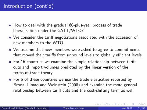
How to deal with the gradual 60-plus-year process of tradeliberalization under the GATT/WTO?
We consider the tari¤ negotiations associated with the accession ofnew members to the WTO.
We assume that new members were asked to agree to commitmentsthat moved their tari¤s from unbound levels to globally e¢ cient levels.
For 16 countries we examine the simple relationship between tari¤cuts and import volumes predicted by the linear version of theterms-of-trade theory.
For 5 of these countries we use the trade elasticities reported byBroda, Limao and Weinstein (2008) and examine the more generalrelationship between tari¤ cuts and the cost-shifting term as well.
Bagwell and Staiger (Stanford University) Trade Negotiations June 2009 5 / 30
Introduction (cont�d)
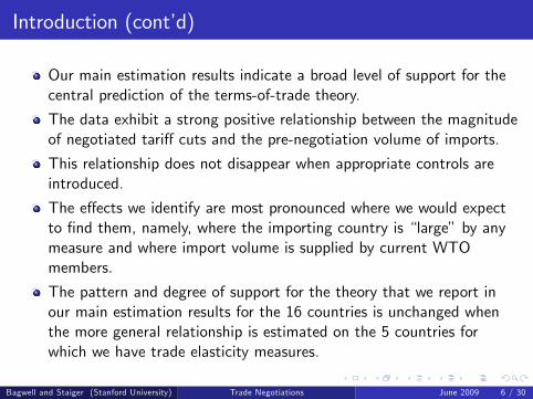
Our main estimation results indicate a broad level of support for thecentral prediction of the terms-of-trade theory.
The data exhibit a strong positive relationship between the magnitudeof negotiated tari¤ cuts and the pre-negotiation volume of imports.
This relationship does not disappear when appropriate controls areintroduced.
The e¤ects we identify are most pronounced where we would expectto �nd them, namely, where the importing country is �large�by anymeasure and where import volume is supplied by current WTOmembers.
The pattern and degree of support for the theory that we report inour main estimation results for the 16 countries is unchanged whenthe more general relationship is estimated on the 5 countries forwhich we have trade elasticity measures.
Bagwell and Staiger (Stanford University) Trade Negotiations June 2009 6 / 30

Theory
A simple multi-country multi-good partial equilibrium setting,developed from the perspective of a particular �domestic� country.
Domestic Demands and Supplies of the product under consideration:
D(p) = α� δ(p), and
S(p) = λ+ κ(p),
with δ/(p) > 0 and κ
/(p) > 0, and with α and λ domestic demand
and supply shifters, respectively.
Volume of domestic imports:
M(p) � D(p)� S(p) = [α� λ]� [δ(p) + κ(p)].
Ad valorem tari¤ τ; pricing relationships p = (1+ τ)pw � p(τ, pw );equilibrium world price p̃w (τ, �).
Bagwell and Staiger (Stanford University) Trade Negotiations June 2009 7 / 30
Theory (cont�d)
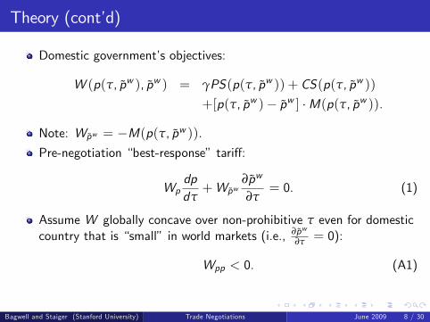
Domestic government�s objectives:
W (p(τ, p̃w ), p̃w ) = γPS(p(τ, p̃w )) + CS(p(τ, p̃w ))
+[p(τ, p̃w )� p̃w ] �M(p(τ, p̃w )).
Note: Wp̃w = �M(p(τ, p̃w )).Pre-negotiation �best-response� tari¤:
Wpdpdτ+Wp̃w
∂p̃w
∂τ= 0. (1)
Assume W globally concave over non-prohibitive τ even for domesticcountry that is �small� in world markets (i.e., ∂p̃w
∂τ = 0):
Wpp < 0. (A1)
Bagwell and Staiger (Stanford University) Trade Negotiations June 2009 8 / 30
Theory (cont�d)
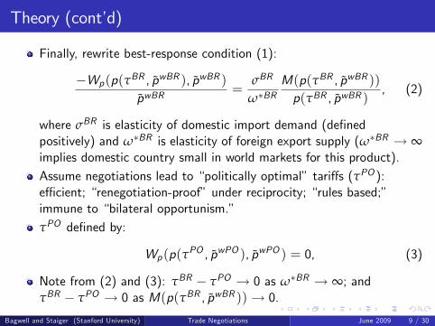
Finally, rewrite best-response condition (1):
�Wp(p(τBR , p̃wBR ), p̃wBR )p̃wBR
=σBR
ω�BRM(p(τBR , p̃wBR ))p(τBR , p̃wBR )
, (2)
where σBR is elasticity of domestic import demand (de�nedpositively) and ω�BR is elasticity of foreign export supply (ω�BR ! ∞implies domestic country small in world markets for this product).Assume negotiations lead to �politically optimal� tari¤s (τPO ):e¢ cient; �renegotiation-proof�under reciprocity; �rules based;�immune to �bilateral opportunism.�τPO de�ned by:
Wp(p(τPO , p̃wPO ), p̃wPO ) = 0, (3)
Note from (2) and (3): τBR � τPO ! 0 as ω�BR ! ∞; andτBR � τPO ! 0 as M(p(τBR , p̃wBR ))! 0.
Bagwell and Staiger (Stanford University) Trade Negotiations June 2009 9 / 30
Theory (cont�d)
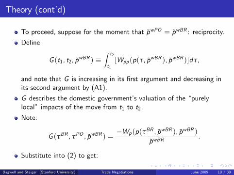
To proceed, suppose for the moment that p̃wPO = p̃wBR : reciprocity.
De�ne
G (t1, t2, p̃wBR ) �Z t2
t1[Wpp(p(τ, p̃wBR ), p̃wBR )]dτ,
and note that G is increasing in its �rst argument and decreasing inits second argument by (A1).
G describes the domestic government�s valuation of the �purelylocal� impacts of the move from t1 to t2.
Note:
G (τBR , τPO , p̃wBR ) =�Wp(p(τBR , p̃wBR ), p̃wBR )
p̃wBR.
Substitute into (2) to get:
Bagwell and Staiger (Stanford University) Trade Negotiations June 2009 10 / 30

Theory (cont�d)
An equilibrium relationship between τBR and τPO :
G (τBR , τPO , p̃wBR ) =σBR
ω�BRM(p(τBR , p̃wBR ))p(τBR , p̃wBR )
. (4)
Note: all magnitudes on RHS of (4) are measured at the�pre-negotiation stage;� and recall that G is decreasing in its secondargument.
Fix τBR , p̃wBR and the function G and compare goods 1 and 2;
if (σBR
ω�BRM(p(τBR , p̃wBR ))p(τBR , p̃wBR )
)1 > (σBR
ω�BRM(p(τBR , p̃wBR ))p(τBR , p̃wBR )
)2,
then (τBR � τPO )1 > (τBR � τPO )2.
Bagwell and Staiger (Stanford University) Trade Negotiations June 2009 11 / 30
Theory (cont�d)
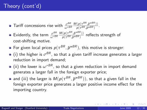
Tari¤ concessions rise with σBR
ω�BRM (p(τBR ,p̃wBR ))p(τBR ,p̃wBR ) .
Evidently, the term σBR
ω�BRM (p(τBR ,p̃wBR ))p(τBR ,p̃wBR ) re�ects strength of
cost-shifting motive.
For given local prices p(τBR , p̃wBR ), this motive is stronger:
(i) the higher is σBR , so that a given tari¤ increase generates a largerreduction in import demand;
(ii) the lower is ω�BR , so that a given reduction in import demandgenerates a larger fall in the foreign exporter price;
and (iii) the larger is M(p(τBR , p̃wBR )), so that a given fall in theforeign exporter price generates a larger positive income e¤ect for theimporting country.
Bagwell and Staiger (Stanford University) Trade Negotiations June 2009 12 / 30
Theory (cont�d)
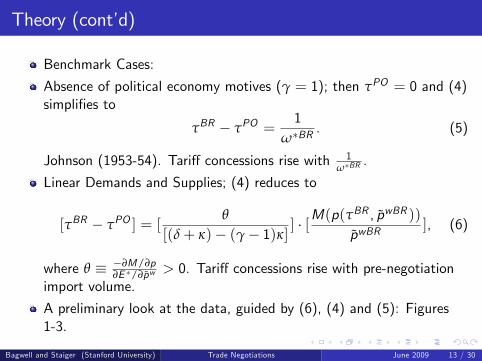
Benchmark Cases:
Absence of political economy motives (γ = 1); then τPO = 0 and (4)simpli�es to
τBR � τPO =1
ω�BR . (5)
Johnson (1953-54). Tari¤ concessions rise with 1ω�BR .
Linear Demands and Supplies; (4) reduces to
[τBR � τPO ] = [θ
[(δ+ κ)� (γ� 1)κ] ] � [M(p(τBR , p̃wBR ))
p̃wBR], (6)
where θ � �∂M/∂p∂E �/∂p̃w > 0. Tari¤ concessions rise with pre-negotiation
import volume.
A preliminary look at the data, guided by (6), (4) and (5): Figures1-3.
Bagwell and Staiger (Stanford University) Trade Negotiations June 2009 13 / 30
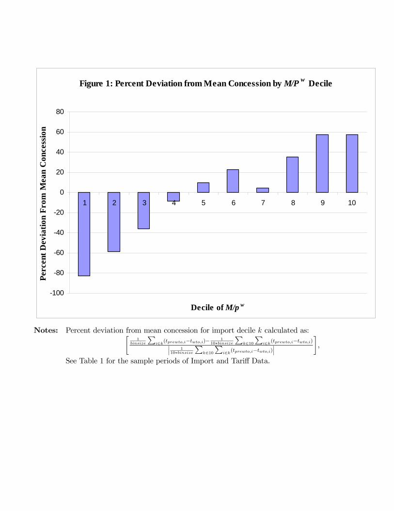
Figure 1: Percent Deviation from Mean Concession by M/P w Decile
-100
-80
-60
-40
-20
0
20
40
60
80
1 2 3 4 5 6 7 8 9 10
Decile of M/p w
Perc
ent D
evia
tion
From
Mea
n C
once
ssio
n
Notes: Percent deviation from mean concession for import decile k calculated as:�1
binsize
Pi2k(tprewto;i�twto;i)�
110�binsize
Pk210
Pi2k(tprewto;i�twto;i)��� 1
10�binsize
Pk210
Pi2k(tprewto;i�twto;i)
����,
See Table 1 for the sample periods of Import and Tari¤ Data.
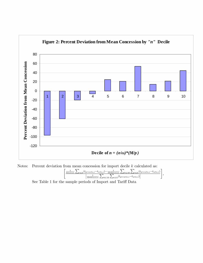
Figure 2: Percent Deviation from Mean Concession by "n" Decile
-120
-100
-80
-60
-40
-20
0
20
40
60
80
1 2 3 4 5 6 7 8 9 10
Decile of n = ( )*(M/p )
Perc
ent D
evia
tion
from
Mea
n C
once
ssio
n
Notes: Percent deviation from mean concession for import decile k calculated as:�1
binsize
Pi2k(tprewto;i�twto;i)�
110�binsize
Pk210
Pi2k(tprewto;i�twto;i)��� 1
10�binsize
Pk210
Pi2k(tprewto;i�twto;i)
����,
See Table 1 for the sample periods of Import and Tari¤ Data
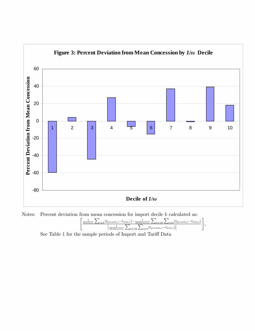
Figure 3: Percent Deviation from Mean Concession by 1/ Decile
-80
-60
-40
-20
0
20
40
60
1 2 3 4 5 6 7 8 9 10
Decile of 1/
Perc
ent D
evia
tion
from
Mea
n C
once
ssio
n
Notes: Percent deviation from mean concession for import decile k calculated as:�1
binsize
Pi2k(tprewto;i�twto;i)�
110�binsize
Pk210
Pi2k(tprewto;i�twto;i)��� 1
10�binsize
Pk210
Pi2k(tprewto;i�twto;i)
����,
See Table 1 for the sample periods of Import and Tari¤ Data
Theory (cont�d)
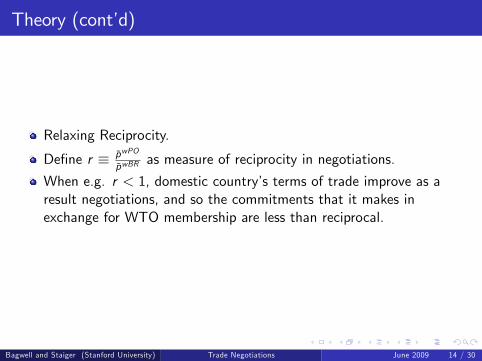
Relaxing Reciprocity.
De�ne r � p̃wPO
p̃wBR as measure of reciprocity in negotiations.
When e.g. r < 1, domestic country�s terms of trade improve as aresult negotiations, and so the commitments that it makes inexchange for WTO membership are less than reciprocal.
Bagwell and Staiger (Stanford University) Trade Negotiations June 2009 14 / 30

Theory (cont�d)
Generalization of the Linear Benchmark (6) allowing for the possibilityof non-reciprocal tari¤ negotiations:
τPO � τBR = β0 + (β1 � 1)τBR + β2[M(p(τBR , p̃wBR ))
p̃wBR],
where
β0 =(γ� 1)(r � 1)κ
[(δ+ κ)� (γ� 1)rκ] , with β0 S 0 as r S 1,
β1 =[(δ+ κ)� (γ� 1)κ][(δ+ κ)� (γ� 1)rκ] , with β1 > 0 and β1 S 1 as r S 1, and
β2 = [�θ
[(δ+ κ)� (γ� 1)rκ] ], with β2 < 0.
Bagwell and Staiger (Stanford University) Trade Negotiations June 2009 15 / 30
Theory (cont�d)
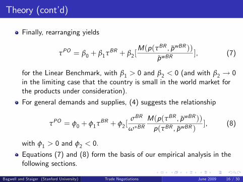
Finally, rearranging yields
τPO = β0 + β1τBR + β2[
M(p(τBR , p̃wBR ))p̃wBR
], (7)
for the Linear Benchmark, with β1 > 0 and β2 < 0 (and with β2 ! 0in the limiting case that the country is small in the world market forthe products under consideration).
For general demands and supplies, (4) suggests the relationship
τPO = φ0 + φ1τBR + φ2[
σBR
ω�BRM(p(τBR , p̃wBR ))p(τBR , p̃wBR )
], (8)
with φ1 > 0 and φ2 < 0.
Equations (7) and (8) form the basis of our empirical analysis in thefollowing sections.
Bagwell and Staiger (Stanford University) Trade Negotiations June 2009 16 / 30

Empirical Strategy
Estimate equations of the form
τWTOgc = β0 + β1τBRgc + β2m
BRgc + εgc , and (9)
τWTOgc = φ0 + φ1τBRgc + φ2n
BRgc + υgc , (10)
where:
g indexes HS 6-digit products and c indexes countries;
τWTOgc is the ad valorem tari¤ level bound by country c on product gin a GATT/WTO negotiation and τBRgc is country c�s pre-negotiationad valorem tari¤ level on product c ;
mBR � [M (p(τBR ,p̃wBR ))p̃wBR ] and nBR � [ σBR
ω�BRM (p(τBR ,p̃wBR ))p(τBR ,p̃wBR ) ]; and
εgc and υgc are error terms.
Bagwell and Staiger (Stanford University) Trade Negotiations June 2009 17 / 30

Empirical Strategy (cont�d)
Obstacles.
Gradual Trade Liberalization: Focus on Accession of new WTOmembers.
Measurement of τBRgc : use pre-negotiation ad valorem tari¤s for mainresults, but check robustness with NTB AVE measures from Kee,Nicita and Olarreaga (2009) for 8 of our 16 countries.
Measurement of σBR and ω�BR : focus on simpler relationshippredicted by Linear Benchmark for main results, but check robustnessby estimating general relationship with trade elasticity measures fromBroda, Limao and Weinstein (2008) for 5 of our 16 countries.
Controlling for di¤erences across products/countries indemand/supply slopes, political economy parameters and reciprocityin negotiations: include country and industry �xed e¤ects, and reportestimates on sub-samples of observations grouped by country and byindustrial sector.
Bagwell and Staiger (Stanford University) Trade Negotiations June 2009 18 / 30

Data and Descriptive Statistics
16 of the 21 countries that joined the WTO between January 1, 1995and November 2005.
All tari¤ data comes from TRAINS data set (ad valorem 6-digit HSlevel).
Import value data comes from PCTAS data base (subset ofCOMTRADE data base), collected at 6-digit HS level and averagedover 1995-1999. Convert to quantity data with unit values fromCOMTRADE.
Table 1; Table 2; Table 3a-b.
Bagwell and Staiger (Stanford University) Trade Negotiations June 2009 19 / 30
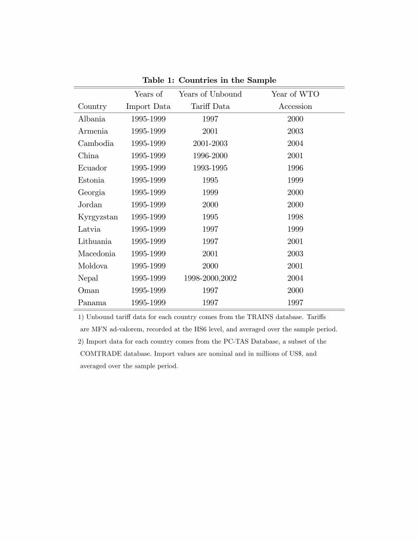
Table 1: Countries in the Sample
Years of Years of Unbound Year of WTO
Country Import Data Tari¤ Data Accession
Albania 1995-1999 1997 2000
Armenia 1995-1999 2001 2003
Cambodia 1995-1999 2001-2003 2004
China 1995-1999 1996-2000 2001
Ecuador 1995-1999 1993-1995 1996
Estonia 1995-1999 1995 1999
Georgia 1995-1999 1999 2000
Jordan 1995-1999 2000 2000
Kyrgyzstan 1995-1999 1995 1998
Latvia 1995-1999 1997 1999
Lithuania 1995-1999 1997 2001
Macedonia 1995-1999 2001 2003
Moldova 1995-1999 2000 2001
Nepal 1995-1999 1998-2000,2002 2004
Oman 1995-1999 1997 2000
Panama 1995-1999 1997 1997
1) Unbound tari¤ data for each country comes from the TRAINS database. Tari¤s
are MFN ad-valorem, recorded at the HS6 level, and averaged over the sample period.
2) Import data for each country comes from the PC-TAS Database, a subset of the
COMTRADE database. Import values are nominal and in millions of US$, and
averaged over the sample period.

Table 2: Industry Description by 1-digit HS SectorHS Description
Live Animals; Meat and Edible Meat O¤al; Fish and Crustaceans, Molluscs and Other Aquatic Invertebrates; Dairy Produce;
Birds�Eggs; Natural Honey; Products of Animal Origin, Not Elsewhere Speci�ed or Included; Live Trees and Other Plants;
0 Bulbs, Roots and the Like; Cut Flowers and Ornamental Foliage; Edible Vegetables and Certain Roots and Tubers;
Edible Fruit and Nuts; Peel of Citrus Fruit or Melons; Co¤ee, Tea, Maté and Spices
Cereals; Products of the Milling Industry; Malt; Starches; Insulin; Oil Seeds and Oleaginous Fruits; Miscellaneous Grains,
Seeds and Fruit; Industrial or Medicinal Plants; Straw and Fodder; Lac; Gums, Resins and Other Vegetable Saps and Extracts;
1 Vegetable Plaiting Materials; Vegetable Products Not Elsewhere Speci�ed or Included; Animal or Vegetable Fats and Oils
and Their Cleavage Products; Pastrycooks�Products; Preparations of Meat, of Fish or of Crustaceans, Molluscs or Other
Aquatic Invertebrates; Sugars and Sugar Confectionery; Wheat Gluten; Cocoa and Cocoa Preparations; Preparations of
Cereals, Flour, Starch or Milk; Prepared Edible Fats; Animal or Vegetable Waxes.
Preparations of Vegetables, Fruit, Nuts or Other Parts of Plants; Miscellaneous Edible Preparations; Beverages, Spirits and
Vinegar; Residues and Waste From the Food Industries; Prepared Animal Fodder; Tobacco and Manufactured Tobacco
2 Substitutes; Salt; Sulphur; Earths and Stone; Plastering Materials, Lime and Cement; Ores, Slag and Ash; Mineral Fuels,
Mineral Oils and Products of Their Distillation; Organic or Inorganic Compounds of Precious Metals, of Rare-Earth Metals, of
Radioactive Elements or of Isotopes; Organic Chemicals Bituminous Substances; Mineral Waxes; Inorganic Chemicals;
Pharmaceutical Products; Fertilisers; Tanning or Dyeing Extracts; Tannins and Their Derivatives; Dyes, Pigments and
Other Colouring Matter; Paints and Varnishes; Putty and Other Mastics; Inks; Essential Oils and Resinoids; Perfumery,
3 Cosmetics or Toilet Preparations; Soap, Organic Surface-active Agents, Washing Preparations, Lubricating Preparations,
Arti�cial Waxes, Prepared Waxes, Polishing or Scouring Preparations, Candles and Similar Articles, Modelling Pastes,
"Dental Waxes" and Dental Preparations with a Basis of Plaster Albuminoidal Substances; Modi�ed Starches; Glues;
Enzymes; Explosives; Pyrotechnic Products; Matches; Pyrophoric Alloys; Certain Combustible Preparations;
Photographic or Cinematographic Goods; Miscellaneous Chemical Products; Plastics and Articles Thereof
Rubber and Articles Thereof; Raw Hides and Skins (Other Than Furskins) and Leather; Articles of Leather; Travel Goods,
Handbags and Similar Containers; Saddlery and Harness; Articles of Animal Gut (Other Than Silk-Worm Gut); Furskins and
4 Arti�cial Fur; Manufactures Thereof; Wood and Articles of Wood; Wood Charcoal; Cork and Articles of Cork; Manufactures
of Straw, of Esparto or of Other Plaiting Materials; Basketware and Wickerwork; Pulp of Wood or of Other Fibrous Cellulosic
Material; Waste and Scrap of Paper or Paperboard; Paper and Paperboard; Printed Books, Newspapers, Pictures and Other
Products of the Printing Industry; Manuscripts, Typescripts and Plans; Articles of Paper Pulp, of Paper or of Paperboard;
Silk; Wool, Fine or Coarse Animal Hair; Horsehair Yarn and Woven Fabric; Cotton; Other Vegetable Textile Fibres; Paper Yarn
and Woven Fabrics of Paper Yarn; Man-Made Filaments; Man-Made Staple Fibres; Wadding, Felt and Nonwovens; Special
5 Yarns; Twine; Cordage, Ropes and Cables and Articles Thereof; Carpets and Other Textile Floor Coverings; Carpets and
Other Textile Floor Coverings; Special Woven Fabrics; Tufted Textile Fabrics; Lace; Tapestries; Trimmings; Embroidery;
Impregnated, Coated, Covered or Laminated Textile Fabrics; Textile Articles of a Kind Suitable For Industrial Use
Knitted or Crocheted Fabrics; Articles of Apparel and Clothing Accessories, Knitted or Crocheted; Articles of Apparel and
Clothing Accessories, Not Knitted or Crocheted; Other Made Up Textile Articles; Sets; Worn Clothing and Worn Textile Articles;
6 Rags; Footwear, Gaiters and the Like; Parts of Such Articles; Headgear and Parts Thereof; Umbrellas, Sun Umbrellas,
Walking-Sticks, Seat-Sticks, Whips, Riding-Crops and Parts Thereof;Prepared Feathers and Down and Articles Made of Feathers
or of Down; Arti�cial Flowers; Articles of Human Hair; Articles of Stone, Plaster, Cement, Asbestos, Mica or Similar Materials;
Ceramic Products; Glass and Glassware
Glass and Glassware; Natural or Cultured Pearls, Precious or Semi-Precious Stones, Precious Metals, Metals Clad with Precious
7 Metal, and Articles Thereof; Imitation Jewellery; Coin; Iron and Steel; Articles of Iron or Steel; Copper and Articles Thereof;
Nickel and Articles Thereof; Aluminum and Articles Thereof; Lead and Articles Thereof; Zinc and Articles Thereof
Tin and Articles Thereof; Other Base Metals; Cermets and Articles Thereof; Tools, Implements, Cutlery, Spoons and Forks,
of Base Metal; Parts Thereof of Base Metal; Miscellaneous Articles of Base Metal; Nuclear Reactors, Boilers, Machinery and
Mechanical Appliances; Parts Thereof; Electrical Machinery and Equipment and Parts Thereof; Sound Recorders and Reproducers,
8 Television Image and Sound Recorders and Reproducers, and Parts and Accessories of Such ArticlesRailway or Tramway
Locomotives, Rolling- Stock and Parts Thereof; Railway or Tramway Track Fixtures and Fittings and Parts Thereof; Mechanical
(Including Electro-Mechanical) Tra¢ c Signalling Equipment of all Kinds; Vehicles Other Than Railway or Tramway Rolling-Stock,
and Parts and Accessories Thereof; Airraft, Spacecraft, and Parts Thereof; Ships, Boats and Floating Structures
Optical, Photographic, Cinematographic, Measuring, Checking, Precision, Medical or Surgical Instruments and Apparatus; Parts and
Accessories Thereof Clocks and Watches and Parts Thereof; Musical Instruments; Parts and Accessories of Such Articles; Arms
9 and Ammunition; Parts and Accessories Thereof Furniture; Bedding, Mattresses, Mattress Supports, Cushions and Similar Stu¤ed
Furnishings; Lamps and Lighting Fittings, Not Elsewhere Speci�ed or Included; Illuminated Signs, Illuminated Name-Plates and the
Like; Prefabricated Buildings; Toys, Games and Sports Requisites; Parts and Accessories Thereof; Miscellaneous Manufactured
Articles; Works of Art, Collectors�Pieces and Antiques
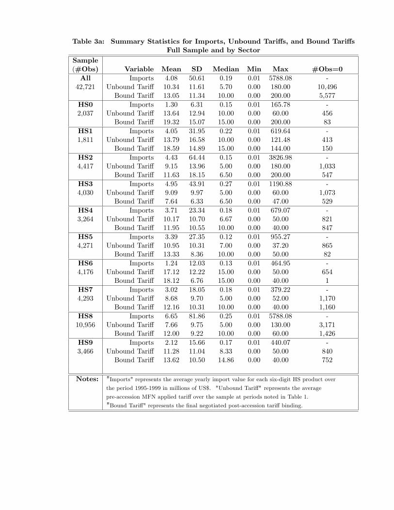
Table 3a: Summary Statistics for Imports, Unbound Tari¤s, and Bound Tari¤sFull Sample and by Sector
Sample(#Obs) Variable Mean SD Median Min Max #Obs=0All Imports 4.08 50.61 0.19 0.01 5788.08 -42,721 Unbound Tari¤ 10.34 11.61 5.70 0.00 180.00 10,496
Bound Tari¤ 13.05 11.34 10.00 0.00 200.00 5,577HS0 Imports 1.30 6.31 0.15 0.01 165.78 -2,037 Unbound Tari¤ 13.64 12.94 10.00 0.00 60.00 456
Bound Tari¤ 19.32 15.07 15.00 0.00 200.00 83HS1 Imports 4.05 31.95 0.22 0.01 619.64 -1,811 Unbound Tari¤ 13.79 16.58 10.00 0.00 121.48 413
Bound Tari¤ 18.59 14.89 15.00 0.00 144.00 150HS2 Imports 4.43 64.44 0.15 0.01 3826.98 -4,417 Unbound Tari¤ 9.15 13.96 5.00 0.00 180.00 1,033
Bound Tari¤ 11.63 18.15 6.50 0.00 200.00 547HS3 Imports 4.95 43.91 0.27 0.01 1190.88 -4,030 Unbound Tari¤ 9.09 9.97 5.00 0.00 60.00 1,073
Bound Tari¤ 7.64 6.33 6.50 0.00 47.00 529HS4 Imports 3.71 23.34 0.18 0.01 679.07 -3,264 Unbound Tari¤ 10.17 10.70 6.67 0.00 50.00 821
Bound Tari¤ 11.95 10.55 10.00 0.00 40.00 847HS5 Imports 3.39 27.35 0.12 0.01 955.27 -4,271 Unbound Tari¤ 10.95 10.31 7.00 0.00 37.20 865
Bound Tari¤ 13.33 8.36 10.00 0.00 50.00 82HS6 Imports 1.24 12.03 0.13 0.01 464.95 -4,176 Unbound Tari¤ 17.12 12.22 15.00 0.00 50.00 654
Bound Tari¤ 18.12 6.76 15.00 0.00 40.00 1HS7 Imports 3.02 18.05 0.18 0.01 379.22 -4,293 Unbound Tari¤ 8.68 9.70 5.00 0.00 52.00 1,170
Bound Tari¤ 12.16 10.31 10.00 0.00 40.00 1,160HS8 Imports 6.65 81.86 0.25 0.01 5788.08 -10,956 Unbound Tari¤ 7.66 9.75 5.00 0.00 130.00 3,171
Bound Tari¤ 12.00 9.22 10.00 0.00 60.00 1,426HS9 Imports 2.12 15.66 0.17 0.01 440.07 -3,466 Unbound Tari¤ 11.28 11.04 8.33 0.00 50.00 840
Bound Tari¤ 13.62 10.50 14.86 0.00 40.00 752
Notes: "Imports" represents the average yearly import value for each six-digit HS product overthe period 1995-1999 in millions of US$. "Unbound Tari¤" represents the average
pre-accession MFN applied tari¤ over the sample at periods noted in Table 1.
"Bound Tari¤" represents the �nal negotiated post-accession tari¤ binding.
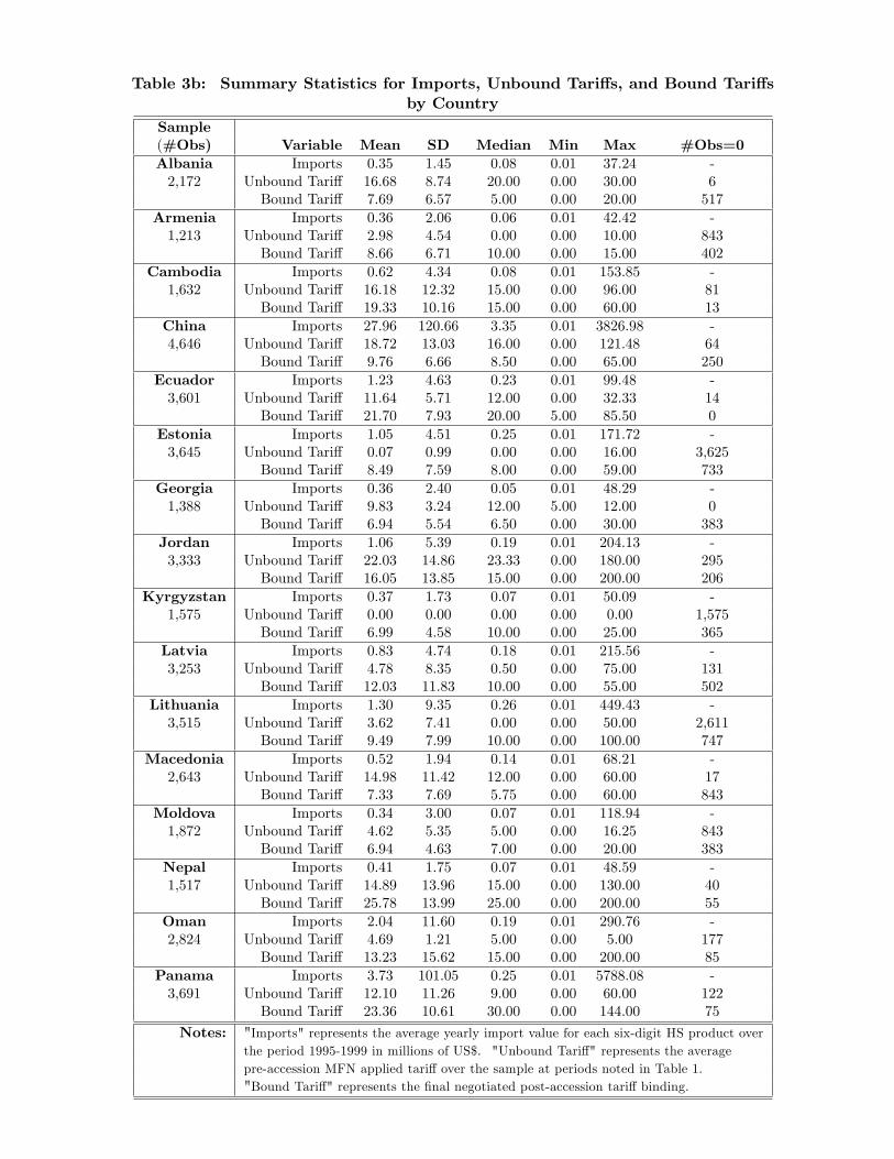
Table 3b: Summary Statistics for Imports, Unbound Tari¤s, and Bound Tari¤sby Country
Sample(#Obs) Variable Mean SD Median Min Max #Obs=0Albania Imports 0.35 1.45 0.08 0.01 37.24 -2,172 Unbound Tari¤ 16.68 8.74 20.00 0.00 30.00 6
Bound Tari¤ 7.69 6.57 5.00 0.00 20.00 517Armenia Imports 0.36 2.06 0.06 0.01 42.42 -1,213 Unbound Tari¤ 2.98 4.54 0.00 0.00 10.00 843
Bound Tari¤ 8.66 6.71 10.00 0.00 15.00 402Cambodia Imports 0.62 4.34 0.08 0.01 153.85 -1,632 Unbound Tari¤ 16.18 12.32 15.00 0.00 96.00 81
Bound Tari¤ 19.33 10.16 15.00 0.00 60.00 13China Imports 27.96 120.66 3.35 0.01 3826.98 -4,646 Unbound Tari¤ 18.72 13.03 16.00 0.00 121.48 64
Bound Tari¤ 9.76 6.66 8.50 0.00 65.00 250Ecuador Imports 1.23 4.63 0.23 0.01 99.48 -3,601 Unbound Tari¤ 11.64 5.71 12.00 0.00 32.33 14
Bound Tari¤ 21.70 7.93 20.00 5.00 85.50 0Estonia Imports 1.05 4.51 0.25 0.01 171.72 -3,645 Unbound Tari¤ 0.07 0.99 0.00 0.00 16.00 3,625
Bound Tari¤ 8.49 7.59 8.00 0.00 59.00 733Georgia Imports 0.36 2.40 0.05 0.01 48.29 -1,388 Unbound Tari¤ 9.83 3.24 12.00 5.00 12.00 0
Bound Tari¤ 6.94 5.54 6.50 0.00 30.00 383Jordan Imports 1.06 5.39 0.19 0.01 204.13 -3,333 Unbound Tari¤ 22.03 14.86 23.33 0.00 180.00 295
Bound Tari¤ 16.05 13.85 15.00 0.00 200.00 206Kyrgyzstan Imports 0.37 1.73 0.07 0.01 50.09 -
1,575 Unbound Tari¤ 0.00 0.00 0.00 0.00 0.00 1,575Bound Tari¤ 6.99 4.58 10.00 0.00 25.00 365
Latvia Imports 0.83 4.74 0.18 0.01 215.56 -3,253 Unbound Tari¤ 4.78 8.35 0.50 0.00 75.00 131
Bound Tari¤ 12.03 11.83 10.00 0.00 55.00 502Lithuania Imports 1.30 9.35 0.26 0.01 449.43 -3,515 Unbound Tari¤ 3.62 7.41 0.00 0.00 50.00 2,611
Bound Tari¤ 9.49 7.99 10.00 0.00 100.00 747Macedonia Imports 0.52 1.94 0.14 0.01 68.21 -
2,643 Unbound Tari¤ 14.98 11.42 12.00 0.00 60.00 17Bound Tari¤ 7.33 7.69 5.75 0.00 60.00 843
Moldova Imports 0.34 3.00 0.07 0.01 118.94 -1,872 Unbound Tari¤ 4.62 5.35 5.00 0.00 16.25 843
Bound Tari¤ 6.94 4.63 7.00 0.00 20.00 383Nepal Imports 0.41 1.75 0.07 0.01 48.59 -1,517 Unbound Tari¤ 14.89 13.96 15.00 0.00 130.00 40
Bound Tari¤ 25.78 13.99 25.00 0.00 200.00 55Oman Imports 2.04 11.60 0.19 0.01 290.76 -2,824 Unbound Tari¤ 4.69 1.21 5.00 0.00 5.00 177
Bound Tari¤ 13.23 15.62 15.00 0.00 200.00 85Panama Imports 3.73 101.05 0.25 0.01 5788.08 -3,691 Unbound Tari¤ 12.10 11.26 9.00 0.00 60.00 122
Bound Tari¤ 23.36 10.61 30.00 0.00 144.00 75
Notes: "Imports" represents the average yearly import value for each six-digit HS product overthe period 1995-1999 in millions of US$. "Unbound Tari¤" represents the averagepre-accession MFN applied tari¤ over the sample at periods noted in Table 1."Bound Tari¤" represents the �nal negotiated post-accession tari¤ binding.
Data and Descriptive Statistics (cont�d)
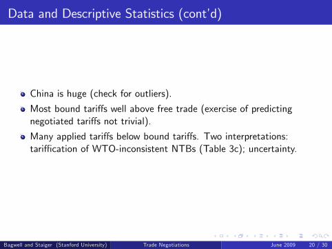
China is huge (check for outliers).
Most bound tari¤s well above free trade (exercise of predictingnegotiated tari¤s not trivial).
Many applied tari¤s below bound tari¤s. Two interpretations:tari¢ cation of WTO-inconsistent NTBs (Table 3c); uncertainty.
Bagwell and Staiger (Stanford University) Trade Negotiations June 2009 20 / 30

Table 3c: Comparison of Unbound Tari¤s, NTB�s, and Bound Tari¤s
Unbound Tari¤ Unbound Tari¤ Bound Tari¤ #Obs
+ NTB
All 9.80 16.67 10.67 25,302
HS0 12.48 28.50 18.45 1,339
HS1 14.57 25.21 17.73 1,081
HS2 8.64 14.42 10.30 2,765
HS3 8.40 15.72 6.15 2,312
HS4 9.08 15.33 8.63 1,956
HS5 11.46 14.99 10.31 2,604
HS6 17.40 24.19 15.82 2,472
HS7 7.91 13.40 9.13 2,480
HS8 6.45 13.80 9.00 6,281
HS9 10.66 15.66 10.68 2,012
Albania 16.70 17.35 7.71 2,187
China 18.72 25.07 9.76 4,645
Estonia 0.07 0.67 8.53 3,613
Jordan 22.03 45.73 16.05 3,332
Latvia 4.78 11.89 12.03 3,253
Lithuania 3.62 9.23 9.49 3,514
Moldova 4.63 6.83 6.95 1,871
Oman 4.69 9.87 13.23 2,824
Notes "Unbound Tari¤" represents the average pre-accession MFN applied tari¤ over the sample
at periods noted in Table 1. "NTB" represents the average ad-valorem equivalent NTB
measure as described in Kee, Nicita, and Olarreaga (2009). "Bound Tari¤" represents
the �nal negotiated post-accession tari¤ binding.
Main Results
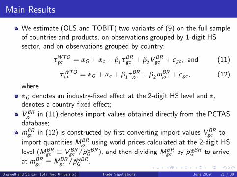
We estimate (OLS and TOBIT) two variants of (9) on the full sampleof countries and products, on observations grouped by 1-digit HSsector, and on observations grouped by country:
τWTOgc = αG + αc + β1τBRgc + β2V
BRgc + εgc , and (11)
τWTOgc = αG + αc + β1τBRgc + β2m
BRgc + εgc , (12)
whereαG denotes an industry-�xed e¤ect at the 2-digit HS level and αcdenotes a country-�xed e¤ect;V BRgc in (11) denotes import values obtained directly from the PCTASdatabase;mBRgc in (12) is constructed by �rst converting import values V BRgc toimport quantities MBR
gc using world prices calculated at the 2-digit HSlevel (MBR
gc � V BRgc /p̃wBRG ), and then dividing MBRgc by p̃wBRG to arrive
at mBRgc � MBRgc /p̃wBRG .
Bagwell and Staiger (Stanford University) Trade Negotiations June 2009 21 / 30
Main Results (cont�d)
Table 4a: Estimates on observations over the full sample and groupedby 1-digit HS sector.
Strong support for theory.
Table 4b: Estimates on observations grouped by country.
Weaker support for theory; but note that Cambodia and Nepal, theonly countries in our 16 that acceded under special LDC rules, look�anomalous,� as they should.
Table 4c: Estimates on observations grouped by country for a singlesector (HS8); Modest improvement over Table 4b.
Bagwell and Staiger (Stanford University) Trade Negotiations June 2009 22 / 30

Table 4a: Baseline Results - Full Sample, by Sector
Equation: τwtogc = αG + αc + β1τ
BRgc + β2
[V BR
gc
]+ εgc τwto
gc = αG + αc + β1τBRgc + β2
[mBR
gc
]+ vgc
OLS Tobit OLSa Tobita
Sample Obs β1 β2 R2 β1 β2 Obs β1 β2 R2 β1 β2
All 42,721 0.3702*** -0.0044*** 0.804 0.3901*** -0.0065*** 42,015 0.3682*** -0.0026*** 0.802 0.3873*** -0.0028**(0.0174) (0.0008) (0.0051) (0.0010) (0.0178) (0.0009) (0.0052) (0.0012)
HS0 2,037 0.3750*** -0.0733** 0.763 0.3925*** -0.0657 2,037 0.3760*** -0.0391** 0.763 0.3934*** -0.0395(0.0284) (0.0338) (0.0291) (0.0443) (0.0283) (0.0180) (0.0291) (0.0332)
HS1 1,811 0.2226*** -0.0476*** 0.783 0.2376*** -0.0487*** 1,811 0.2234*** -0.1558*** 0.783 0.2397*** -0.1643***(0.0311) (0.0104) (0.0218) (0.0095) (0.0308) (0.0278) (0.0218) (0.0297)
HS2 4,417 0.6502*** -0.0001 0.651 0.6781*** -0.0053 4,377 0.6513*** -0.0273*** 0.651 0.6787*** -0.0304*(0.0707) (0.0015) (0.0210) (0.0051) (0.0707) (0.0095) (0.0210) (0.0175)
HS3 4,030 0.2679*** -0.0044*** 0.868 0.2805*** -0.0047*** 4,030 0.2680*** -0.0029*** 0.868 0.2806*** -0.0029(0.0162) (0.0008) (0.0098) (0.0015) (0.0162) (0.0011) (0.0098) (0.0027)
HS4 3,264 0.3285*** -0.0059*** 0.919 0.3711*** -0.0061 3,264 0.3284*** -0.0102*** 0.919 0.3709*** -0.0114(0.0142) (0.0017) (0.0147) (0.0048) (0.0142) (0.0031) (0.0147) (0.0102)
HS5 4,271 0.3136*** -0.0055*** 0.955 0.3163*** -0.0055*** 4,271 0.3134*** -0.0167*** 0.955 0.3162*** -0.0169***(0.0104) (0.0015) (0.0083) (0.0020) (0.0104) (0.0045) (0.0083) (0.0064)
HS6 4,176 0.1342*** -0.0134*** 0.974 0.1342*** -0.0134*** 4,176 0.1336*** -0.0101 0.974 0.1335*** -0.0101***(0.0144) (0.0044) (0.0089) (0.0041) (0.0144) (0.0065) (0.0089) (0.0026)
HS7 4,293 0.3705*** -0.0111*** 0.906 0.3763*** -0.0088 4,061 0.3245*** -0.0020 0.903 0.3225*** 0.0056(0.0185) (0.0025) (0.0153) (0.0057) (0.0205) (0.0032) (0.0172) (0.0098)
HS8 10,956 0.4013*** -0.0044*** 0.872 0.4144*** -0.0057*** 10,955 0.4015*** -0.0159*** 0.872 0.4145*** -0.0191***(0.0159) (0.0006) (0.0080) (0.0008) (0.0159) (0.0026) (0.0080) (0.0029)
HS9 3,466 0.3715*** -0.0112* 0.886 0.4123*** -0.0113 3,033 0.3783*** -0.0928** 0.887 0.4184*** -0.1139***(0.0176) (0.0063) (0.0179) (0.0082) (0.0186) (0.0381) (0.0189) (0.0263)
Notes: Standard errors are in parentheses (OLS are heteroskedasticity-robust). The labels *, **, and *** denote significance at the 10%, 5%,
and 1% level, respectively. Industry fixed effects, αG, are at the two-digit HS product level.
Country fixed effects are denoted by αc. Fixed effect estimates are available upon request. The term τwtogc represents
the final negotiated post-accession tariff binding. The term τBRgc represents the average pre-accession MFN applied tariff over the
sample at periods noted in Table 1. The term V BRgc is the average yearly import value for each six-digit HS product over the
period 1995-1999. The term pwBRG is the total value of imports divided by the total quantity of imports over all sample countries,
for each two-digit HS product, averaged over the period 1995-1999. mBRgc is calculated by dividing the V BR
gc by(pwBR
G
)2, g ∈ G.
a) The variable mBRgc was rescaled dividing it by the corresponding sample mean.
1
Main Results (cont�d)
Table 4a: Estimates on observations over the full sample and groupedby 1-digit HS sector.
Strong support for theory.
Table 4b: Estimates on observations grouped by country.
Weaker support for theory; but note that Cambodia and Nepal, theonly countries in our 16 that acceded under special LDC rules, look�anomalous,� as they should.
Table 4c: Estimates on observations grouped by country for a singlesector (HS8); Modest improvement over Table 4b.
Bagwell and Staiger (Stanford University) Trade Negotiations June 2009 22 / 30
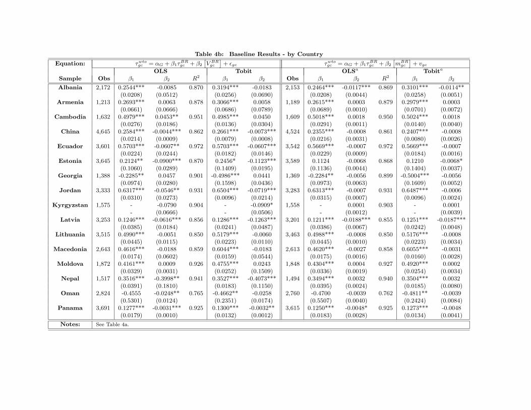
Table 4b: Baseline Results - by Country
Equation: τwtogc = αG + β1τ
BRgc + β2
[V BR
gc
]+ εgc τwto
gc = αG + β1τBRgc + β2
[mBR
gc
]+ vgc
OLS Tobit OLSa Tobita
Sample Obs β1 β2 R2 β1 β2 Obs β1 β2 R2 β1 β2
Albania 2,172 0.2544*** -0.0085 0.870 0.3194*** -0.0183 2,153 0.2464*** -0.0117*** 0.869 0.3101*** -0.0114**(0.0208) (0.0512) (0.0256) (0.0690) (0.0208) (0.0044) (0.0258) (0.0051)
Armenia 1,213 0.2693*** 0.0063 0.878 0.3066*** 0.0058 1,189 0.2615*** 0.0003 0.879 0.2979*** 0.0003(0.0661) (0.0666) (0.0686) (0.0789) (0.0689) (0.0010) (0.0701) (0.0072)
Cambodia 1,632 0.4979*** 0.0453** 0.951 0.4985*** 0.0450 1,609 0.5018*** 0.0018 0.950 0.5024*** 0.0018(0.0276) (0.0186) (0.0136) (0.0304) (0.0291) (0.0011) (0.0140) (0.0040)
China 4,645 0.2584*** -0.0044*** 0.862 0.2661*** -0.0073*** 4,524 0.2355*** -0.0008 0.861 0.2407*** -0.0008(0.0214) (0.0009) (0.0079) (0.0008) (0.0216) (0.0031) (0.0080) (0.0026)
Ecuador 3,601 0.5703*** -0.0607** 0.972 0.5703*** -0.0607*** 3,542 0.5669*** -0.0007 0.972 0.5669*** -0.0007(0.0224) (0.0244) (0.0182) (0.0146) (0.0229) (0.0009) (0.0184) (0.0016)
Estonia 3,645 0.2124** -0.0900*** 0.870 0.2456* -0.1123*** 3,589 0.1124 -0.0068 0.868 0.1210 -0.0068*(0.1060) (0.0289) (0.1409) (0.0195) (0.1136) (0.0044) (0.1404) (0.0037)
Georgia 1,388 -0.2285** 0.0457 0.901 -0.4986*** 0.0441 1,369 -0.2284** -0.0056 0.899 -0.5004*** -0.0056(0.0974) (0.0280) (0.1598) (0.0436) (0.0973) (0.0063) (0.1609) (0.0052)
Jordan 3,333 0.6317*** -0.0546** 0.931 0.6504*** -0.0719*** 3,283 0.6313*** -0.0007 0.931 0.6487*** -0.0006(0.0310) (0.0273) (0.0096) (0.0214) (0.0315) (0.0007) (0.0096) (0.0024)
Kyrgyzstan 1,575 - -0.0790 0.904 - -0.0909* 1,558 - 0.0001 0.903 - 0.0001- (0.0666) - (0.0506) - (0.0012) - (0.0039)
Latvia 3,253 0.1246*** -0.0616*** 0.856 0.1286*** -0.1263*** 3,201 0.1211*** -0.0188*** 0.855 0.1251*** -0.0187***(0.0385) (0.0184) (0.0241) (0.0487) (0.0386) (0.0067) (0.0242) (0.0048)
Lithuania 3,515 0.4990*** -0.0051 0.850 0.5179*** -0.0060 3,463 0.4988*** -0.0008 0.850 0.5176*** -0.0008(0.0445) (0.0115) (0.0223) (0.0110) (0.0445) (0.0010) (0.0223) (0.0034)
Macedonia 2,643 0.4616*** -0.0188 0.859 0.6044*** -0.0183 2,613 0.4620*** -0.0027 0.858 0.6055*** -0.0031(0.0174) (0.0602) (0.0159) (0.0544) (0.0175) (0.0016) (0.0160) (0.0028)
Moldova 1,872 0.4161*** 0.0009 0.926 0.4755*** 0.0243 1,848 0.4304*** 0.0004 0.927 0.4920*** 0.0002(0.0329) (0.0031) (0.0252) (0.1509) (0.0336) (0.0019) (0.0254) (0.0034)
Nepal 1,517 0.3516*** -0.3998** 0.941 0.3527*** -0.4073*** 1,494 0.3494*** 0.0032 0.940 0.3504*** 0.0032(0.0391) (0.1810) (0.0183) (0.1150) (0.0395) (0.0024) (0.0185) (0.0080)
Oman 2,824 -0.4555 -0.0248** 0.765 -0.4662** -0.0258 2,760 -0.4700 -0.0039 0.762 -0.4811** -0.0039(0.5301) (0.0124) (0.2351) (0.0174) (0.5507) (0.0040) (0.2424) (0.0084)
Panama 3,691 0.1277*** -0.0031*** 0.925 0.1300*** -0.0032** 3,615 0.1250*** -0.0048* 0.925 0.1273*** -0.0048(0.0179) (0.0010) (0.0132) (0.0012) (0.0183) (0.0028) (0.0134) (0.0041)
Notes: See Table 4a.
1

Main Results (cont�d)
Table 4a: Estimates on observations over the full sample and groupedby 1-digit HS sector.
Strong support for theory.
Table 4b: Estimates on observations grouped by country.
Weaker support for theory; but note that Cambodia and Nepal, theonly countries in our 16 that acceded under special LDC rules, look�anomalous,� as they should.
Table 4c: Estimates on observations grouped by country for a singlesector (HS8); Modest improvement over Table 4b.
Bagwell and Staiger (Stanford University) Trade Negotiations June 2009 22 / 30

Table 4c: Baseline Results – Country-Specific β2 Estimates – HS8
τwtogc = αG + αc + β1τ
BRgc +
∑c∈C
βc2
[V BR
gc
]+ εgc
OLS Tobit
β1 0.4065*** 0.4192***(0.016) (0.008)
βAlbania2 0.3627 0.3612
(0.287) (0.381)βArmenia
2 -0.9192*** -1.5141***(0.224) (0.512)
βCambodia2 0.0103 -0.0025
(0.066) (0.110)
βChina2 -0.0030*** -0.0056***
(0.0007) (0.001)
βEcuador2 -0.0790** -0.0821**
(0.039) (0.033)βEstonia
2 -0.1338*** -0.2007***(0.025) (0.043)
βGeorgia2 -0.5376** -1.3584
(0.267) (0.864)
βJordan2 -0.1100** -0.1231***
(0.048) (0.047)
βKyrgyzstan2 -0.5340*** -0.7652**
(0.190) (0.352)βLatvia
2 0.0599 0.0531(0.086) (0.084)
βLithuania2 -0.0298 -0.0293
(0.019) (0.033)
βMacedonia2 -0.1715* -0.1627
(0.103) (0.135)
βMoldova2 0.1951 0.1454
(0.330) (0.525)
βNepal2 -1.2159** -1.2773***
(0.583) (0.199)βOman
2 -0.0063 -0.0071(0.008) (0.012)
βPanama2 -0.0054*** -0.0056***
(0.001) (0.001)
Obs. 10,956 10,956R2 0.873
Notes See Tables 4a and 4b
Main Results (cont�d)
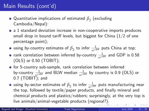
Quantitative implications of estimated β2 (excludingCambodia/Nepal):
a 1 standard deviation increase in non-cooperative imports producessmall drop in bound tari¤ levels, but biggest for China (1/2 of onepercentage point);
using by-country estimates of β2 to infer1
ω�BR puts China at top;
rank correlation between inferred by-country 1ω�BR and GDP is 0.58
(OLS) or 0.50 (TOBIT);
for 5-country sub-sample, rank correlation between inferredby-country 1
ω�BR and BLW median 1ω�BR by country is 0.9 (OLS) or
0.7 (TOBIT); and
using by-sector estimates of β2 to infer1
ω�BR puts manufacturing nearthe top, followed by textile/paper products, and �nally mineral andchemical products and plastics/rubbers; surprisingly, at the very top islive animals/animal-vegetable products (regional?).
Bagwell and Staiger (Stanford University) Trade Negotiations June 2009 23 / 30
Main Results (cont�d)
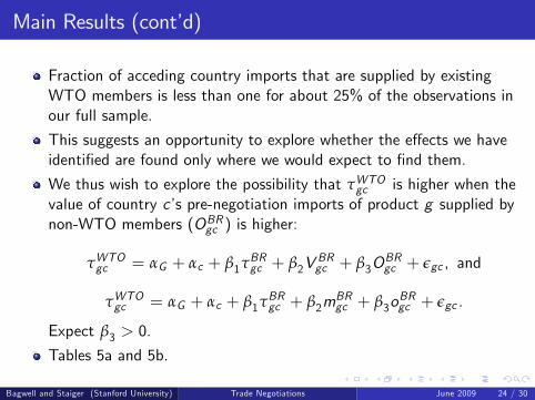
Fraction of acceding country imports that are supplied by existingWTO members is less than one for about 25% of the observations inour full sample.
This suggests an opportunity to explore whether the e¤ects we haveidenti�ed are found only where we would expect to �nd them.
We thus wish to explore the possibility that τWTOgc is higher when thevalue of country c�s pre-negotiation imports of product g supplied bynon-WTO members (OBRgc ) is higher:
τWTOgc = αG + αc + β1τBRgc + β2V
BRgc + β3O
BRgc + εgc , and
τWTOgc = αG + αc + β1τBRgc + β2m
BRgc + β3o
BRgc + εgc .
Expect β3 > 0.
Tables 5a and 5b.
Bagwell and Staiger (Stanford University) Trade Negotiations June 2009 24 / 30

Table 5a: Extended Results using Import Values
Equation: τwtogc = αG + αc + βtijprewto + β2[V BR
gc ] + β3[OBRgc ] + εgc
OLS TobitSample Obs β1 β2 β3 R2 β1 β2 β3
All 42,721 0.3705*** -0.0058*** 0.0114** 0.804 0.3902*** -0.0073*** 0.0079(0.0174) (0.0015) (0.0046) (0.0051) (0.0011) (0.0059)
HS0 2,037 0.3738*** -0.1281*** 0.1512** 0.763 0.3913*** -0.1195** 0.1483(0.0284) (0.0495) (0.0630) (0.0291) (0.0593) (0.1088)
HS1 1,811 0.2223*** -0.0439*** -0.2083* 0.783 0.2373*** -0.0443*** -0.2506(0.0311) (0.0104) (0.1127) (0.0218) (0.0100) (0.1830)
HS2 4,417 0.6504*** 0.0031 -0.0102 0.651 0.6781*** -0.0041 -0.0039(0.0707) (0.0070) (0.0183) (0.0210) (0.0089) (0.0241)
HS3 4,030 0.2679*** -0.0037*** -0.0025 0.868 0.2804*** -0.0039 -0.0030(0.0162) (0.0013) (0.0036) (0.0098) (0.0024) (0.0069)
HS4 3,264 0.3285*** -0.0062** 0.0012 0.919 0.371*** -0.0048 -0.0055(0.0142) (0.0030) (0.0087) (0.0147) (0.0083) (0.0278)
HS5 4,271 0.3134*** -0.0079*** 0.0084 0.955 0.3162*** -0.0076** 0.0074(0.0104) (0.0022) (0.0070) (0.0083) (0.0039) (0.0114)
HS6 4,176 0.1342*** -0.0152 0.0058 0.974 0.1341*** -0.0152** 0.0058(0.0144) (0.0093) (0.0206) (0.0089) (0.0068) (0.0175)
HS7 4,293 0.3703*** -0.0173*** 0.0190*** 0.906 0.3761*** -0.0160* 0.02200(0.0185) (0.0042) (0.0069) (0.0153) (0.0089) (0.0209)
HS8 10,956 0.4014*** -0.0046*** 0.0029 0.872 0.4138*** -0.0049*** -0.0235*(0.0159) (0.0007) (0.0085) (0.0080) (0.0009) (0.0128)
HS9 3,466 0.3709*** -0.0321*** 0.2074*** 0.887 0.4114*** -0.0395*** 0.2656***(0.0176) (0.0083) (0.0449) (0.0178) (0.0136) (0.0996)
Albania 2,187 0.2544*** -0.0185 0.6477 0.871 0.3193*** -0.0251 0.4582(0.0208) (0.0550) (0.6738) (0.0254) (0.0722) (1.4982)
Armenia 1,213 0.2701*** 0.0325 -0.0810 0.878 0.3075*** 0.0378 -0.0961(0.0661) (0.0888) (0.1091) (0.0686) (0.0982) (0.1754)
Cambodia 1,632 0.4978*** 0.0449** -2.4031** 0.951 0.4983*** 0.0446 -2.3953(0.0276) (0.0186) (1.2068) (0.0136) (0.0304) (5.8303)
China 4,646 0.2595*** -0.0064*** 0.0108** 0.862 0.267*** -0.0090*** 0.0102**(0.0212) (0.0014) (0.0043) (0.0079) (0.0011) (0.0045)
Ecuador 3,601 0.57*** -0.0626** 0.0417 0.972 0.57*** -0.0626*** 0.0417(0.0223) (0.0281) (0.2121) (0.0182) (0.0161) (0.1491)
Estonia 3,645 0.2449** -0.1543*** 0.1613*** 0.870 0.3106** -0.2288*** 0.2660***(0.1043) (0.0339) (0.0617) (0.1414) (0.0337) (0.0605)
Georgia 1,388 -0.2285** 0.0455 0.0026 0.901 -0.4986*** 0.0431 0.0114(0.0974) (0.0304) (0.0488) (0.1598) (0.0456) (0.1516)
Jordan 3,333 0.6312*** -0.1142*** 0.1128*** 0.931 0.6499*** -0.1661*** 0.1646***(0.0310) (0.0261) (0.0270) (0.0095) (0.0340) (0.0454)
Kyrgyzstan 1,575 - -0.6273*** 0.6686*** 0.906 - -0.7916*** 0.8343***- (0.1382) (0.1458) - (0.1545) (0.1706)
Latvia 3,253 0.1243*** -0.2290*** 0.2680*** 0.857 0.1281*** -0.3668*** 0.3913***(0.0383) (0.0737) (0.0963) (0.0240) (0.0852) (0.1174)
Lithuania 3,515 0.5004*** -0.0680** 0.0776*** 0.850 0.5197*** -0.0931*** 0.1034***(0.0444) (0.0286) (0.0294) (0.0223) (0.0301) (0.0332)
Macedonia 2,643 0.4617*** -0.0272 0.2825 0.859 0.6044*** -0.0266 0.3435(0.0174) (0.0575) (0.4633) (0.0159) (0.0564) (0.6144)
Moldova 1,872 0.4164*** 0.0343 -0.0351 0.926 0.4753*** 0.0417 -0.1408(0.0329) (0.0843) (0.0857) (0.0252) (0.1674) (0.5872)
Nepal 1,517 0.3537*** -0.6204*** 1.8017** 0.941 0.3548*** -0.6343*** 1.8511**(0.0391) (0.2107) (0.8526) (0.0183) (0.1518) (0.8096)
Oman 2,824 -0.4571 -0.0213* -0.2186* 0.765 -0.4677** -0.0225 -0.2101(0.5303) (0.0113) (0.1251) (0.2351) (0.0178) (0.2459)
Panama 3,691 0.128*** -0.0019 -0.1304 0.925 0.1303*** -0.0019 -0.1326***(0.0179) (0.0012) (0.0821) (0.0132) (0.0013) (0.0478)
Notes: See Table 4 notes. The term OBRgc is the average yearly import value from non-WTO members
at the time of accession for each six-digit HS product over the period 1995-1999.Country fixed effects are included only for the full-sample and by-sector estimates.
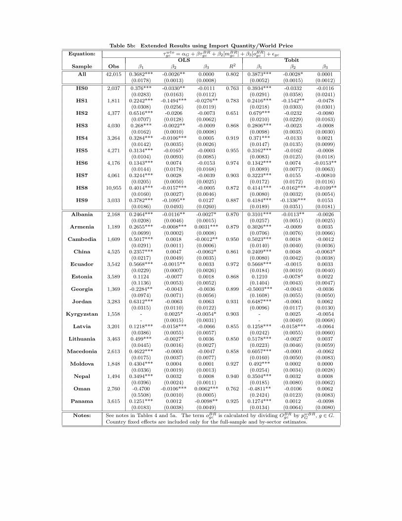
Table 5b: Extended Results using Import Quantity/World Price
Equation: τwtogc = αG + βτBR
gc + β2[mBRgc ] + β3[oBR
gc ] + εgc
OLS TobitSample Obs β1 β2 β3 R2 β1 β2 β3
All 42,015 0.3682*** -0.0026** 0.0000 0.802 0.3873*** -0.0028* 0.0001(0.0178) (0.0013) (0.0008) (0.0052) (0.0015) (0.0012)
HS0 2,037 0.376*** -0.0330** -0.0111 0.763 0.3934*** -0.0332 -0.0116(0.0283) (0.0163) (0.0112) (0.0291) (0.0358) (0.0241)
HS1 1,811 0.2242*** -0.1494*** -0.0276** 0.783 0.2416*** -0.1542** -0.0478(0.0308) (0.0256) (0.0119) (0.0218) (0.0303) (0.0301)
HS2 4,377 0.6516*** -0.0206 -0.0073 0.651 0.679*** -0.0232 -0.0080(0.0707) (0.0128) (0.0062) (0.0210) (0.0229) (0.0163)
HS3 4,030 0.268*** -0.0022** -0.0009 0.868 0.2806*** -0.0023 -0.0008(0.0162) (0.0010) (0.0008) (0.0098) (0.0035) (0.0030)
HS4 3,264 0.3284*** -0.0106*** 0.0005 0.919 0.371*** -0.0133 0.0021(0.0142) (0.0035) (0.0026) (0.0147) (0.0135) (0.0099)
HS5 4,271 0.3134*** -0.0165* -0.0003 0.955 0.3162*** -0.0162 -0.0008(0.0104) (0.0093) (0.0085) (0.0083) (0.0125) (0.0118)
HS6 4,176 0.1343*** 0.0074 -0.0153 0.974 0.1342*** 0.0074 -0.0153**(0.0144) (0.0178) (0.0168) (0.0089) (0.0077) (0.0063)
HS7 4,061 0.3244*** 0.0028 -0.0039 0.903 0.3223*** 0.0155 -0.00810(0.0205) (0.0050) (0.0025) (0.0172) (0.0172) (0.0116)
HS8 10,955 0.4014*** -0.0157*** -0.0005 0.872 0.4141*** -0.0162*** -0.0109**(0.0160) (0.0027) (0.0046) (0.0080) (0.0032) (0.0054)
HS9 3,033 0.3782*** -0.1095** 0.0127 0.887 0.4184*** -0.1336*** 0.0153(0.0186) (0.0493) (0.0260) (0.0189) (0.0351) (0.0181)
Albania 2,168 0.2464*** -0.0116** -0.0027* 0.870 0.3101*** -0.0113** -0.0026(0.0208) (0.0046) (0.0015) (0.0257) (0.0051) (0.0025)
Armenia 1,189 0.2655*** -0.0008*** 0.0031*** 0.879 0.3026*** -0.0009 0.0035(0.0699) (0.0002) (0.0008) (0.0706) (0.0076) (0.0066)
Cambodia 1,609 0.5017*** 0.0018 -0.0012** 0.950 0.5023*** 0.0018 -0.0012(0.0291) (0.0011) (0.0006) (0.0140) (0.0040) (0.0036)
China 4,525 0.2357*** 0.0047 -0.0062* 0.861 0.2409*** 0.0048 -0.0063*(0.0217) (0.0049) (0.0035) (0.0080) (0.0042) (0.0038)
Ecuador 3,542 0.5668*** -0.0015** 0.0033 0.972 0.5668*** -0.0015 0.0033(0.0229) (0.0007) (0.0026) (0.0184) (0.0019) (0.0040)
Estonia 3,589 0.1124 -0.0077 0.0018 0.868 0.1210 -0.0078* 0.0022(0.1136) (0.0053) (0.0052) (0.1404) (0.0043) (0.0047)
Georgia 1,369 -0.2284** -0.0043 -0.0036 0.899 -0.5003*** -0.0043 -0.0036(0.0974) (0.0071) (0.0056) (0.1608) (0.0055) (0.0050)
Jordan 3,283 0.6312*** -0.0063 0.0063 0.931 0.6487*** -0.0061 0.0062(0.0315) (0.0110) (0.0122) (0.0096) (0.0117) (0.0130)
Kyrgyzstan 1,558 - 0.0025* -0.0054* 0.903 - 0.0025 -0.0054- (0.0015) (0.0031) - (0.0049) (0.0068)
Latvia 3,201 0.1218*** -0.0158*** -0.0066 0.855 0.1258*** -0.0158*** -0.0064(0.0386) (0.0055) (0.0057) (0.0242) (0.0055) (0.0060)
Lithuania 3,463 0.499*** -0.0027* 0.0036 0.850 0.5178*** -0.0027 0.0037(0.0445) (0.0016) (0.0027) (0.0223) (0.0046) (0.0059)
Macedonia 2,613 0.4622*** -0.0003 -0.0047 0.858 0.6057*** -0.0001 -0.0062(0.0175) (0.0037) (0.0077) (0.0160) (0.0050) (0.0083)
Moldova 1,848 0.4304*** 0.0004 0.0001 0.927 0.492*** 0.0002 0.0000(0.0336) (0.0019) (0.0013) (0.0254) (0.0034) (0.0028)
Nepal 1,494 0.3494*** 0.0032 0.0008 0.940 0.3504*** 0.0032 0.0008(0.0396) (0.0024) (0.0011) (0.0185) (0.0080) (0.0062)
Oman 2,760 -0.4700 -0.0106*** 0.0062*** 0.762 -0.4811** -0.0106 0.0062(0.5508) (0.0010) (0.0005) (0.2424) (0.0123) (0.0083)
Panama 3,615 0.1251*** 0.0012 -0.0098** 0.925 0.1274*** 0.0012 -0.0098(0.0183) (0.0038) (0.0049) (0.0134) (0.0064) (0.0080)
Notes: See notes in Tables 4 and 5a. The term oBRgc is calculated by dividing OBR
gc by pwBRG , g ∈ G.
Country fixed effects are included only for the full-sample and by-sector estimates.
Robustness
We present estimates that shed light on the potential importance of:
outlier observations (Table 6a/6b);
accounting for Chinese �processing� trade and for the overallin�uence of China (Table 6a/6b); and
alternative approaches to measuring a country�s non-cooperativebest-response tari¤ τBRgc ; add NTB AVEs of Kee, Nicita and Olarreaga(2009) to ad valorem tari¤s (Table 6c/6d/6e).
Bagwell and Staiger (Stanford University) Trade Negotiations June 2009 25 / 30

Table 6a: Sensitivity Analysis - Full Sample, by Sector
Eqn: τwtogc = αG + αc + β1τBR
gc + β2[ln(V BRgc )] + εgc τwto
gc = αG + αc + β1τBRgc + β2[V BR
gc ] + εgc, Normal ChinaOLS Tobit OLS Tobit
Sample Obs β1 β2 R2 β1 β2 Obs β1 β2 R2 β1 β2
All 42,721 0.3676*** -0.3509*** 0.805 0.3871*** -0.3784*** 42,721 0.3703*** -0.0051*** 0.804 0.3900*** -0.0069***(0.0174) (0.0258) (0.0051) (0.0259) (0.0174) (0.0012) (0.0051) (0.0011)
HS0 2,037 0.3685*** -0.5320*** 0.764 0.3861*** -0.5160*** 2,037 0.3725*** -0.1580** 0.763 0.3899*** -0.1540**(0.0288) (0.1642) (0.0291) (0.1618) (0.0285) (0.0730) (0.0291) (0.0668)
HS1 1,811 0.1925*** -0.7096*** 0.782 0.207*** -0.7723*** 1,811 0.2237*** -0.0614*** 0.783 0.2391*** -0.0633***(0.0282) (0.1475) (0.0207) (0.1566) (0.0310) (0.0120) (0.0218) (0.0117)
HS2 4,417 0.6492*** -0.1978 0.651 0.6775*** -0.2336* 4,417 0.6502*** -0.0001 0.651 0.6781*** -0.0057(0.0708) (0.1336) (0.0210) (0.1251) (0.0707) (0.0023) (0.0210) (0.0060)
HS3 4,030 0.2679*** -0.1578*** 0.868 0.2806*** -0.1868*** 4,030 0.2678*** -0.0043*** 0.868 0.2805*** -0.0043*(0.0161) (0.0365) (0.0098) (0.0400) (0.0162) (0.0016) (0.0098) (0.0024)
HS4 3,264 0.326*** -0.3259*** 0.919 0.3679*** -0.3523*** 3,264 0.3281*** -0.0119*** 0.919 0.3702*** -0.0199*(0.0141) (0.0542) (0.0146) (0.0672) (0.0142) (0.0047) (0.0147) (0.0107)
HS5 4,271 0.3135*** -0.0671* 0.955 0.3162*** -0.0662* 4,271 0.3122*** -0.0221*** 0.955 0.3149*** -0.0222***(0.0104) (0.0387) (0.0083) (0.0345) (0.0104) (0.0036) (0.0083) (0.0068)
HS6 4,176 0.1319*** -0.1288*** 0.974 0.1319*** -0.1287*** 4,176 0.1324*** -0.0938 0.974 0.1324*** -0.0938***(0.0144) (0.0366) (0.0089) (0.0337) (0.0143) (0.0595) (0.0089) (0.0174)
HS7 4,293 0.3676*** -0.3479*** 0.907 0.3728*** -0.3828*** 4,293 0.3701*** -0.0230*** 0.906 0.3759*** -0.0215**(0.0184) (0.0492) (0.0152) (0.0642) (0.0185) (0.0055) (0.0153) (0.0092)
HS8 10,956 0.4004*** -0.5607*** 0.875 0.4132*** -0.6075*** 10,956 0.4018*** -0.0050*** 0.872 0.4147*** -0.0058***(0.0155) (0.0373) (0.0079) (0.0368) (0.0160) (0.0009) (0.0080) (0.0009)
HS9 3,466 0.3608*** -0.8325*** 0.891 0.3984*** -1.0172*** 3,466 0.3701*** -0.0299* 0.886 0.4108*** -0.0295**(0.0171) (0.0709) (0.0175) (0.0833) (0.0176) (0.0176) (0.0179) (0.0128)
Eqn: τwtogc = αG + αc + β1τBR
gc + β1
[V BR
gc
]+ εgc , No China Notes:
OLS Tobit See Table 4a.Sample Obs β1 β2 R2 β1 β2
All 38,075 0.4201*** -0.0052*** 0.808 0.4471*** -0.0056***(0.0194) (0.0017) (0.0058) (0.0014)
HS0 1,754 0.386*** -0.4607*** 0.760 0.4033*** -0.4595***(0.0331) (0.1165) (0.0342) (0.1311)
HS1 1,600 0.3452*** -0.1478*** 0.792 0.3557*** -0.1898***(0.0385) (0.0358) (0.0296) (0.0599)
HS2 3,718 0.7237*** 0.0356 0.662 0.7567*** 0.0350*(0.0681) (0.0378) (0.0235) (0.0197)
HS3 3,654 0.2577*** -0.0144 0.867 0.2721*** -0.0166(0.0158) (0.0113) (0.0105) (0.0216)
HS4 2,917 0.3352*** -0.2713*** 0.921 0.3768*** -0.2949***(0.0159) (0.0655) (0.0167) (0.0592)
HS5 3,778 0.3313*** -0.0912* 0.956 0.3351*** -0.0974***(0.0125) (0.0533) (0.0096) (0.0295)
HS6 3,750 0.1124*** -0.0779 0.975 0.1124*** -0.0779***(0.0157) (0.0605) (0.0094) (0.0187)
HS7 3,838 0.3171*** -0.0931** 0.908 0.3221*** -0.1017***(0.0201) (0.0369) (0.0178) (0.0337)
HS8 9,972 0.4067*** -0.0057*** 0.875 0.4217*** -0.0059***(0.0181) (0.0015) (0.0091) (0.0010)
HS9 3,094 0.3551*** -0.7004*** 0.895 0.3994*** -0.8203***(0.0183) (0.1218) (0.0184) (0.0865)

Table 6b - Sensitivity Analysis, by Country
Eqn: τwtogc = αG + β1τBR
gc + β2
[ln(V BR
gc )]
+ εgc
OLS TobitSample Obs β1 β2 R2 β1 β2
Albania 2,172 0.254*** 0.0237 0.870 0.3196*** -0.0051(0.0208) (0.0598) (0.0256) (0.0760)
Armenia 1,213 0.2687*** -0.0842 0.878 0.3061*** -0.1130(0.0662) (0.1004) (0.0686) (0.1265)
Cambodia 1,632 0.496*** -0.1532 0.951 0.4965*** -0.1569*(0.0273) (0.1005) (0.0136) (0.0815)
China 4,645 0.2575*** -0.5166*** 0.866 0.2642*** -0.5454***(0.0207) (0.0427) (0.0077) (0.0364)
Ecuador 3,601 0.5643*** -0.2206*** 0.972 0.5643*** -0.2206***(0.0226) (0.0473) (0.0182) (0.0424)
Estonia 3,645 0.1408*** -0.2763*** 0.870 0.1587 -0.3679***(0.1045) (0.0497) (0.1392) (0.0553)
Georgia 1,388 -0.2306** -0.0494 0.901 -0.5032*** -0.0865(0.0973) (0.0630) (0.1599) (0.0793)
Jordan 3,333 0.6316*** -0.2853*** 0.931 0.6507*** -0.3369***(0.0311) (0.0661) (0.0095) (0.0663)
Kyrgyzstan 1,575 - -0.1333** 0.905 - -0.1715**- (0.0530) - (0.0631)
Latvia 3,253 0.1258*** -0.3753*** 0.857 0.13*** -0.4279***(0.0382) (0.0809) (0.0240) (0.0894)
Lithuania 3,515 0.5043*** -0.2736*** 0.851 0.5243*** -0.3348***(0.0441) (0.0584) (0.0223) (0.0661)
Macedonia 2,643 0.4619*** -0.1677*** 0.859 0.604*** -0.2152***(0.0174) (0.0606) (0.0158) (0.0767)
Moldova 1,872 0.4163*** 0.0060 0.926 0.4752*** -0.0001(0.0330) (0.0418) (0.0251) (0.0520)
Nepal 1,517 0.3571*** -0.7666*** 0.942 0.3582*** -0.7764***(0.0383) (0.1545) (0.0182) (0.1363)
Oman 2,824 -0.4799 -0.3222** 0.765 -0.4908 -0.3273***(0.5321) (0.1304) (0.2350) (0.1121)
Panama 3,691 0.1265*** -1.2464*** 0.930 0.1289*** -1.2735***(0.0179) (0.0792) (0.0127) (0.0729)
Eqn: τwtogc = αG + β1τBR
gc + β2
[V BR
gc
]+ εgc, Normal China
OLS TobitSample Obs β1 β2 R2 β1 β2
China-Normal 4,646 0.2589*** -0.0055*** 0.862 0.2669*** -0.0102***(0.0215) (0.0015) (0.0079) (0.0012)
Notes: See Table 4a.
Robustness
We present estimates that shed light on the potential importance of:
outlier observations (Table 6a/6b);
accounting for Chinese �processing� trade and for the overallin�uence of China (Table 6a/6b); and
alternative approaches to measuring a country�s non-cooperativebest-response tari¤ τBRgc ; add NTB AVEs of Kee, Nicita and Olarreaga(2009) to ad valorem tari¤s (Table 6c/6d/6e).
Bagwell and Staiger (Stanford University) Trade Negotiations June 2009 25 / 30
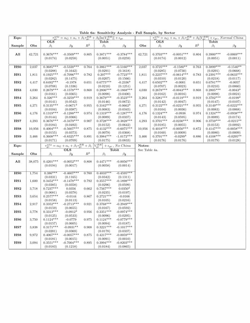
Table 6a: Sensitivity Analysis - Full Sample, by Sector
Eqn: τwtogc = αG + αc + β1τBR
gc + β2[ln(V BRgc )] + εgc τwto
gc = αG + αc + β1τBRgc + β2[V BR
gc ] + εgc, Normal ChinaOLS Tobit OLS Tobit
Sample Obs β1 β2 R2 β1 β2 Obs β1 β2 R2 β1 β2
All 42,721 0.3676*** -0.3509*** 0.805 0.3871*** -0.3784*** 42,721 0.3703*** -0.0051*** 0.804 0.3900*** -0.0069***(0.0174) (0.0258) (0.0051) (0.0259) (0.0174) (0.0012) (0.0051) (0.0011)
HS0 2,037 0.3685*** -0.5320*** 0.764 0.3861*** -0.5160*** 2,037 0.3725*** -0.1580** 0.763 0.3899*** -0.1540**(0.0288) (0.1642) (0.0291) (0.1618) (0.0285) (0.0730) (0.0291) (0.0668)
HS1 1,811 0.1925*** -0.7096*** 0.782 0.207*** -0.7723*** 1,811 0.2237*** -0.0614*** 0.783 0.2391*** -0.0633***(0.0282) (0.1475) (0.0207) (0.1566) (0.0310) (0.0120) (0.0218) (0.0117)
HS2 4,417 0.6492*** -0.1978 0.651 0.6775*** -0.2336* 4,417 0.6502*** -0.0001 0.651 0.6781*** -0.0057(0.0708) (0.1336) (0.0210) (0.1251) (0.0707) (0.0023) (0.0210) (0.0060)
HS3 4,030 0.2679*** -0.1578*** 0.868 0.2806*** -0.1868*** 4,030 0.2678*** -0.0043*** 0.868 0.2805*** -0.0043*(0.0161) (0.0365) (0.0098) (0.0400) (0.0162) (0.0016) (0.0098) (0.0024)
HS4 3,264 0.326*** -0.3259*** 0.919 0.3679*** -0.3523*** 3,264 0.3281*** -0.0119*** 0.919 0.3702*** -0.0199*(0.0141) (0.0542) (0.0146) (0.0672) (0.0142) (0.0047) (0.0147) (0.0107)
HS5 4,271 0.3135*** -0.0671* 0.955 0.3162*** -0.0662* 4,271 0.3122*** -0.0221*** 0.955 0.3149*** -0.0222***(0.0104) (0.0387) (0.0083) (0.0345) (0.0104) (0.0036) (0.0083) (0.0068)
HS6 4,176 0.1319*** -0.1288*** 0.974 0.1319*** -0.1287*** 4,176 0.1324*** -0.0938 0.974 0.1324*** -0.0938***(0.0144) (0.0366) (0.0089) (0.0337) (0.0143) (0.0595) (0.0089) (0.0174)
HS7 4,293 0.3676*** -0.3479*** 0.907 0.3728*** -0.3828*** 4,293 0.3701*** -0.0230*** 0.906 0.3759*** -0.0215**(0.0184) (0.0492) (0.0152) (0.0642) (0.0185) (0.0055) (0.0153) (0.0092)
HS8 10,956 0.4004*** -0.5607*** 0.875 0.4132*** -0.6075*** 10,956 0.4018*** -0.0050*** 0.872 0.4147*** -0.0058***(0.0155) (0.0373) (0.0079) (0.0368) (0.0160) (0.0009) (0.0080) (0.0009)
HS9 3,466 0.3608*** -0.8325*** 0.891 0.3984*** -1.0172*** 3,466 0.3701*** -0.0299* 0.886 0.4108*** -0.0295**(0.0171) (0.0709) (0.0175) (0.0833) (0.0176) (0.0176) (0.0179) (0.0128)
Eqn: τwtogc = αG + αc + β1τBR
gc + β1
[V BR
gc
]+ εgc , No China Notes:
OLS Tobit See Table 4a.Sample Obs β1 β2 R2 β1 β2
All 38,075 0.4201*** -0.0052*** 0.808 0.4471*** -0.0056***(0.0194) (0.0017) (0.0058) (0.0014)
HS0 1,754 0.386*** -0.4607*** 0.760 0.4033*** -0.4595***(0.0331) (0.1165) (0.0342) (0.1311)
HS1 1,600 0.3452*** -0.1478*** 0.792 0.3557*** -0.1898***(0.0385) (0.0358) (0.0296) (0.0599)
HS2 3,718 0.7237*** 0.0356 0.662 0.7567*** 0.0350*(0.0681) (0.0378) (0.0235) (0.0197)
HS3 3,654 0.2577*** -0.0144 0.867 0.2721*** -0.0166(0.0158) (0.0113) (0.0105) (0.0216)
HS4 2,917 0.3352*** -0.2713*** 0.921 0.3768*** -0.2949***(0.0159) (0.0655) (0.0167) (0.0592)
HS5 3,778 0.3313*** -0.0912* 0.956 0.3351*** -0.0974***(0.0125) (0.0533) (0.0096) (0.0295)
HS6 3,750 0.1124*** -0.0779 0.975 0.1124*** -0.0779***(0.0157) (0.0605) (0.0094) (0.0187)
HS7 3,838 0.3171*** -0.0931** 0.908 0.3221*** -0.1017***(0.0201) (0.0369) (0.0178) (0.0337)
HS8 9,972 0.4067*** -0.0057*** 0.875 0.4217*** -0.0059***(0.0181) (0.0015) (0.0091) (0.0010)
HS9 3,094 0.3551*** -0.7004*** 0.895 0.3994*** -0.8203***(0.0183) (0.1218) (0.0184) (0.0865)
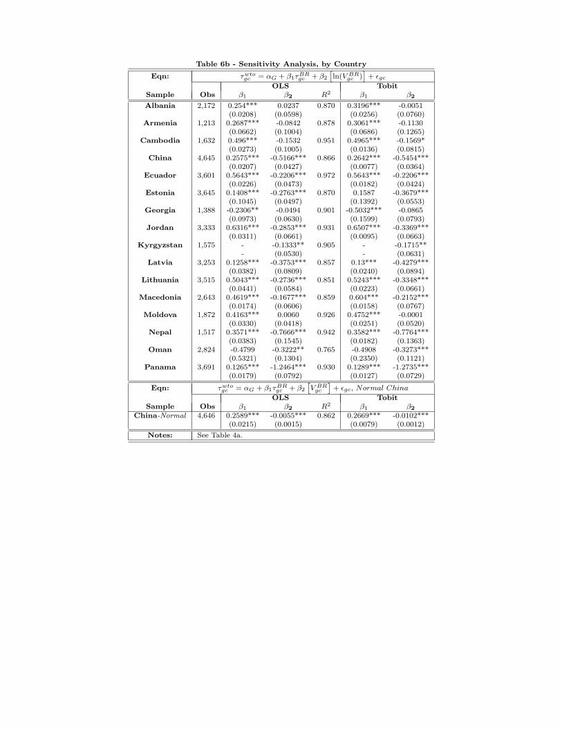
Table 6b - Sensitivity Analysis, by Country
Eqn: τwtogc = αG + β1τBR
gc + β2
[ln(V BR
gc )]
+ εgc
OLS TobitSample Obs β1 β2 R2 β1 β2
Albania 2,172 0.254*** 0.0237 0.870 0.3196*** -0.0051(0.0208) (0.0598) (0.0256) (0.0760)
Armenia 1,213 0.2687*** -0.0842 0.878 0.3061*** -0.1130(0.0662) (0.1004) (0.0686) (0.1265)
Cambodia 1,632 0.496*** -0.1532 0.951 0.4965*** -0.1569*(0.0273) (0.1005) (0.0136) (0.0815)
China 4,645 0.2575*** -0.5166*** 0.866 0.2642*** -0.5454***(0.0207) (0.0427) (0.0077) (0.0364)
Ecuador 3,601 0.5643*** -0.2206*** 0.972 0.5643*** -0.2206***(0.0226) (0.0473) (0.0182) (0.0424)
Estonia 3,645 0.1408*** -0.2763*** 0.870 0.1587 -0.3679***(0.1045) (0.0497) (0.1392) (0.0553)
Georgia 1,388 -0.2306** -0.0494 0.901 -0.5032*** -0.0865(0.0973) (0.0630) (0.1599) (0.0793)
Jordan 3,333 0.6316*** -0.2853*** 0.931 0.6507*** -0.3369***(0.0311) (0.0661) (0.0095) (0.0663)
Kyrgyzstan 1,575 - -0.1333** 0.905 - -0.1715**- (0.0530) - (0.0631)
Latvia 3,253 0.1258*** -0.3753*** 0.857 0.13*** -0.4279***(0.0382) (0.0809) (0.0240) (0.0894)
Lithuania 3,515 0.5043*** -0.2736*** 0.851 0.5243*** -0.3348***(0.0441) (0.0584) (0.0223) (0.0661)
Macedonia 2,643 0.4619*** -0.1677*** 0.859 0.604*** -0.2152***(0.0174) (0.0606) (0.0158) (0.0767)
Moldova 1,872 0.4163*** 0.0060 0.926 0.4752*** -0.0001(0.0330) (0.0418) (0.0251) (0.0520)
Nepal 1,517 0.3571*** -0.7666*** 0.942 0.3582*** -0.7764***(0.0383) (0.1545) (0.0182) (0.1363)
Oman 2,824 -0.4799 -0.3222** 0.765 -0.4908 -0.3273***(0.5321) (0.1304) (0.2350) (0.1121)
Panama 3,691 0.1265*** -1.2464*** 0.930 0.1289*** -1.2735***(0.0179) (0.0792) (0.0127) (0.0729)
Eqn: τwtogc = αG + β1τBR
gc + β2
[V BR
gc
]+ εgc, Normal China
OLS TobitSample Obs β1 β2 R2 β1 β2
China-Normal 4,646 0.2589*** -0.0055*** 0.862 0.2669*** -0.0102***(0.0215) (0.0015) (0.0079) (0.0012)
Notes: See Table 4a.
Robustness
We present estimates that shed light on the potential importance of:
outlier observations (Table 6a/6b);
accounting for Chinese �processing� trade and for the overallin�uence of China (Table 6a/6b); and
alternative approaches to measuring a country�s non-cooperativebest-response tari¤ τBRgc ; add NTB AVEs of Kee, Nicita and Olarreaga(2009) to ad valorem tari¤s (Table 6c/6d/6e).
Bagwell and Staiger (Stanford University) Trade Negotiations June 2009 25 / 30
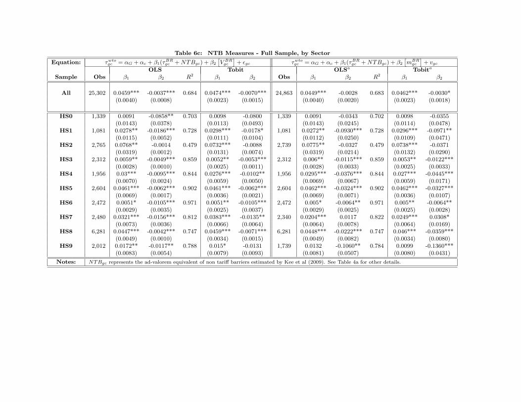
Table 6c: NTB Measures - Full Sample, by Sector
Equation: τwtogc = αG + αc + β1(τ
BRgc +NTBgc) + β2
[V BR
gc
]+ εgc τwto
gc = αG + αc + β1(τBRgc +NTBgc) + β2
[mBR
gc
]+ vgc
OLS Tobit OLSa Tobita
Sample Obs β1 β2 R2 β1 β2 Obs β1 β2 R2 β1 β2
All 25,302 0.0459*** -0.0037*** 0.684 0.0474*** -0.0070*** 24,863 0.0449*** -0.0028 0.683 0.0462*** -0.0030*(0.0040) (0.0008) (0.0023) (0.0015) (0.0040) (0.0020) (0.0023) (0.0018)
HS0 1,339 0.0091 -0.0858** 0.703 0.0098 -0.0800 1,339 0.0091 -0.0343 0.702 0.0098 -0.0355(0.0143) (0.0378) (0.0113) (0.0493) (0.0143) (0.0245) (0.0114) (0.0478)
HS1 1,081 0.0278** -0.0186*** 0.728 0.0298*** -0.0178* 1,081 0.0272** -0.0930*** 0.728 0.0296*** -0.0971**(0.0115) (0.0052) (0.0111) (0.0104) (0.0112) (0.0250) (0.0109) (0.0471)
HS2 2,765 0.0768** -0.0014 0.479 0.0732*** -0.0088 2,739 0.0775** -0.0327 0.479 0.0738*** -0.0371(0.0319) (0.0012) (0.0131) (0.0074) (0.0319) (0.0214) (0.0132) (0.0290)
HS3 2,312 0.0059** -0.0049*** 0.859 0.0052** -0.0053*** 2,312 0.006** -0.0115*** 0.859 0.0053** -0.0122***(0.0028) (0.0010) (0.0025) (0.0011) (0.0028) (0.0033) (0.0025) (0.0033)
HS4 1,956 0.03*** -0.0095*** 0.844 0.0276*** -0.0102** 1,956 0.0295*** -0.0376*** 0.844 0.027*** -0.0445***(0.0070) (0.0024) (0.0059) (0.0050) (0.0069) (0.0067) (0.0059) (0.0171)
HS5 2,604 0.0461*** -0.0062*** 0.902 0.0461*** -0.0062*** 2,604 0.0462*** -0.0324*** 0.902 0.0462*** -0.0327***(0.0069) (0.0017) (0.0036) (0.0021) (0.0069) (0.0071) (0.0036) (0.0107)
HS6 2,472 0.0051* -0.0105*** 0.971 0.0051** -0.0105*** 2,472 0.005* -0.0064** 0.971 0.005** -0.0064**(0.0029) (0.0035) (0.0025) (0.0037) (0.0029) (0.0025) (0.0025) (0.0028)
HS7 2,480 0.0321*** -0.0156*** 0.812 0.0383*** -0.0135** 2,340 0.0204*** 0.0117 0.822 0.0249*** 0.0308*(0.0073) (0.0036) (0.0066) (0.0064) (0.0064) (0.0078) (0.0064) (0.0169)
HS8 6,281 0.0447*** -0.0042*** 0.747 0.0459*** -0.0071*** 6,281 0.0448*** -0.0222*** 0.747 0.046*** -0.0359***(0.0049) (0.0010) (0.0034) (0.0015) (0.0049) (0.0082) (0.0034) (0.0080)
HS9 2,012 0.0172** -0.0117** 0.788 0.015* -0.0131 1,739 0.0132 -0.1060** 0.784 0.0099 -0.1360***(0.0083) (0.0054) (0.0079) (0.0093) (0.0081) (0.0507) (0.0080) (0.0431)
Notes: NTBgc represents the ad-valorem equivalent of non tariff barriers estimated by Kee et al (2009). See Table 4a for other details.
1

Table 6d: NTB Measures - by Country
Equation: τwtogc = αG + β1(τ
BRgc +NTBgc) + β2
[V BR
gc
]+ εgc τwto
gc = αG + β1(τBRgc +NTBgc) + β2
[mBR
gc
]+ vgc
OLS Tobit OLSa Tobita
Sample Obs β1 β2 R2 β1 β2 Obs β1 β2 R2 β1 β2
Albania 2,187 0.0666*** -0.0152 0.863 0.1222*** -0.022 2,168 0.064*** -0.0120*** 0.863 0.1178*** -0.0116**(0.0219) (0.0593) (0.0153) (0.0705) (0.0212) (0.0044) (0.0153) (0.0052)
China 4,645 0.0302*** -0.0042*** 0.831 0.0314*** -0.0068*** 4,524 0.0265*** -0.0007 0.835 0.027*** -0.0008(0.0041) (0.0008) (0.0028) (0.0009) (0.0040) (0.0027) (0.0028) (0.0028)
Estonia 3,613 -0.0028 -0.0856*** 0.869 -0.0037 -0.1068*** 3,557 -0.0034 -0.0069 0.868 -0.0052 -0.0069*(0.0066) (0.0271) (0.0131) (0.0193) (0.0058) (0.0044) (0.0133) (0.0038)
Jordan 3,332 0.0448*** -0.0920*** 0.837 0.0456*** -0.1105*** 3,282 0.0444*** -0.0046*** 0.838 0.0451*** -0.0047(0.0057) (0.0345) (0.0040) (0.0329) (0.0057) (0.0009) (0.0040) (0.0038)
Latvia 3,253 0.0206** -0.0614*** 0.855 0.0225*** -0.1330*** 3,201 0.0215** -0.0202*** 0.855 0.0231*** -0.0202***(0.0088) (0.0193) (0.0057) (0.0500) (0.0088) (0.0065) (0.0057) (0.0048)
Lithuania 3,514 0.0298*** -0.0039 0.822 0.0322*** -0.0047 3,462 0.0301*** -0.0025** 0.821 0.0324*** -0.0026(0.0051) (0.0107) (0.0052) (0.0120) (0.0051) (0.0012) (0.0052) (0.0037)
Moldova 1,871 0.0010 -0.0026 0.911 -0.0013 -0.1694 1,847 0.0003 0.0016 0.911 -0.0024 0.0016(0.0041) (0.0041) (0.0060) (0.1658) (0.0042) (0.0012) (0.0060) (0.0037)
Oman 2,824 -0.0479** -0.0241** 0.766 -0.0497*** -0.0250 2,760 -0.0480** -0.0038 0.764 -0.0498*** -0.0038(0.0191) (0.0123) (0.0113) (0.0173) (0.0191) (0.0027) (0.0114) (0.0084)
Notes: NTBgc represents the ad-valorem equivalent of non tariff barriers estimated by Kee et al (2009). See Table 4a for other details.
1

Table 6e: NTB Measures – Country-Specific β2 Estimates – HS8
τwtogc = αG + αc + β1τ
BRgc +
∑c∈C
βc2
[V BR
gc
]+ εgc
OLS Tobit
β1 0.0445*** 0.0457***(0.005) (0.003)
βAlbania2 0.4044 0.4167
(0.372) (0.397)
βChina2 -0.0039*** -0.0066***
(0.001) (0.001)βEstonia
2 -0.1326*** -0.2018***(0.029) (0.044)
βJordan2 -0.0723 -0.0807*
(0.059) (0.049)βLatvia
2 -0.0440 -0.0590(0.072) (0.088)
βLithuania2 -0.0563* -0.0557
(0.029) (0.034)
βMoldova2 0.0185 -0.0369
(0.389) (0.547)βOman
2 -0.0144** -0.0155(0.007) (0.012)
Obs. 6,281 6,281R2 0.747
Notes NTBgc represents the ad-valorem
equivalent of non tariff barriers
estimated by Kee et al (2009).
See Table 4a for other details.
Robustness (cont�d)
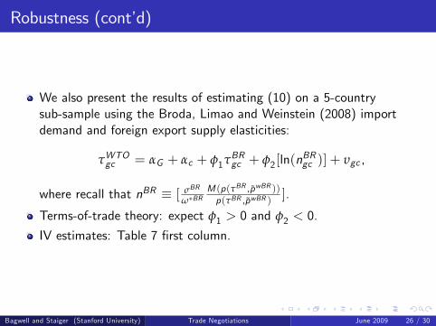
We also present the results of estimating (10) on a 5-countrysub-sample using the Broda, Limao and Weinstein (2008) importdemand and foreign export supply elasticities:
τWTOgc = αG + αc + φ1τBRgc + φ2[ln(n
BRgc )] + υgc ,
where recall that nBR � [ σBR
ω�BRM (p(τBR ,p̃wBR ))p(τBR ,p̃wBR ) ].
Terms-of-trade theory: expect φ1 > 0 and φ2 < 0.
IV estimates: Table 7 �rst column.
Bagwell and Staiger (Stanford University) Trade Negotiations June 2009 26 / 30
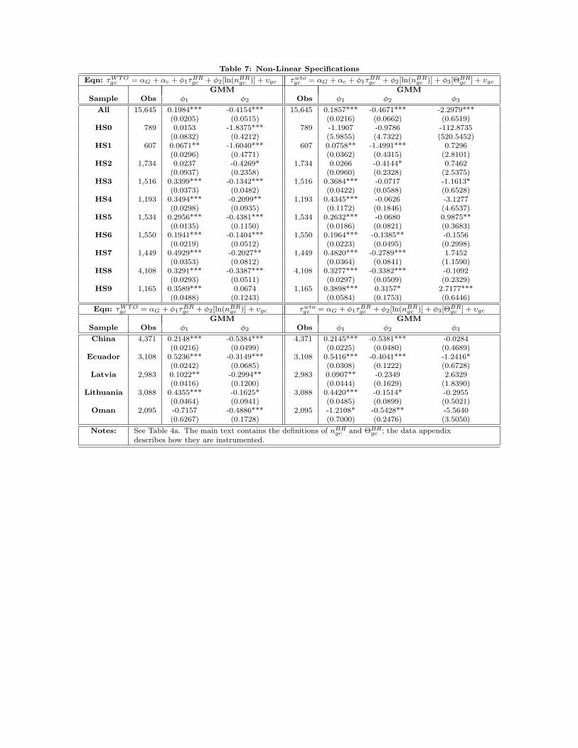
Table 7: Non-Linear Specifications
Eqn: τWTOgc = αG + αc + φ1τBR
gc + φ2[ln(nBRgc )] + υgc τwto
gc = αG + αc + φ1τBRgc + φ2[ln(nBR
gc )] + φ3[ΘBRgc ] + υgc
GMM GMMSample Obs φ1 φ2 Obs φ1 φ2 φ3
All 15,645 0.1984*** -0.4154*** 15,645 0.1857*** -0.4671*** -2.2979***(0.0205) (0.0515) (0.0216) (0.0662) (0.6519)
HS0 789 0.0153 -1.8375*** 789 -1.1907 -0.9786 -112.8735(0.0832) (0.4212) (5.9855) (4.7322) (520.5452)
HS1 607 0.0671** -1.6040*** 607 0.0758** -1.4991*** 0.7296(0.0296) (0.4771) (0.0362) (0.4315) (2.8101)
HS2 1,734 0.0237 -0.4269* 1,734 0.0266 -0.4144* 0.7462(0.0937) (0.2358) (0.0960) (0.2328) (2.5375)
HS3 1,516 0.3399*** -0.1342*** 1,516 0.3684*** -0.0717 -1.1613*(0.0373) (0.0482) (0.0422) (0.0588) (0.6528)
HS4 1,193 0.3494*** -0.2099** 1,193 0.4345*** -0.0626 -3.1277(0.0298) (0.0935) (0.1172) (0.1846) (4.6537)
HS5 1,534 0.2956*** -0.4381*** 1,534 0.2632*** -0.0680 0.9875**(0.0135) (0.1150) (0.0186) (0.0821) (0.3683)
HS6 1,550 0.1941*** -0.1404*** 1,550 0.1964*** -0.1385** -0.1556(0.0219) (0.0512) (0.0223) (0.0495) (0.2998)
HS7 1,449 0.4929*** -0.2027** 1,449 0.4820*** -0.2789*** 1.7452(0.0353) (0.0812) (0.0364) (0.0841) (1.1590)
HS8 4,108 0.3291*** -0.3387*** 4,108 0.3277*** -0.3382*** -0.1092(0.0293) (0.0511) (0.0297) (0.0509) (0.2329)
HS9 1,165 0.3589*** 0.0674 1,165 0.3898*** 0.3157* 2.7177***(0.0488) (0.1243) (0.0584) (0.1753) (0.6446)
Eqn: τWTOgc = αG + φ1τBR
gc + φ2[ln(nBRgc )] + υgc τwto
gc = αG + φ1τBRgc + φ2[ln(nBR
gc )] + φ3[ΘBRgc ] + υgc
GMM GMMSample Obs φ1 φ2 Obs φ1 φ2 φ3
China 4,371 0.2148*** -0.5384*** 4,371 0.2145*** -0.5381*** -0.0284(0.0216) (0.0499) (0.0225) (0.0480) (0.4689)
Ecuador 3,108 0.5236*** -0.3149*** 3,108 0.5416*** -0.4041*** -1.2416*(0.0242) (0.0685) (0.0308) (0.1222) (0.6728)
Latvia 2,983 0.1022** -0.2994** 2,983 0.0907** -0.2349 2.6329(0.0416) (0.1200) (0.0444) (0.1629) (1.8390)
Lithuania 3,088 0.4355*** -0.1625* 3,088 0.4420*** -0.1514* -0.2955(0.0464) (0.0941) (0.0485) (0.0899) (0.5021)
Oman 2,095 -0.7157 -0.4886*** 2,095 -1.2108* -0.5428** -5.5640(0.6267) (0.1728) (0.7000) (0.2476) (3.5050)
Notes: See Table 4a. The main text contains the definitions of nBRgc and ΘBR
gc ; the data appendixdescribes how they are instrumented.
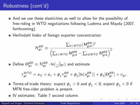
Robustness (cont�d)
And we use these elasticities as well to allow for the possibility offree-riding in WTO negotiations following Ludema and Mayda (2007,forthcoming).
Her�ndahl Index of foreign exporter concentration:
HBRgc �
∑k2WTO (MBRgck )
2�∑k2WTO M
BRgck �∑k /2WTO M
BRgck
�2 .De�ne ΘBR
gc � HBRgc � ln( 1
ω�BR ) and estimate
τWTOgc = αG + αc + φ1τBRgc + φ2[ln(n
BRgc )] + φ3[Θ
BRgc ] + υgc .
Terms-of-trade theory: expect φ1 > 0 and φ2 < 0; expect φ3 < 0 ifMFN free-rider problem is present.
IV estimates: Table 7 second column.
Bagwell and Staiger (Stanford University) Trade Negotiations June 2009 27 / 30

Table 7: Non-Linear Specifications
Eqn: τWTOgc = αG + αc + φ1τBR
gc + φ2[ln(nBRgc )] + υgc τwto
gc = αG + αc + φ1τBRgc + φ2[ln(nBR
gc )] + φ3[ΘBRgc ] + υgc
GMM GMMSample Obs φ1 φ2 Obs φ1 φ2 φ3
All 15,645 0.1984*** -0.4154*** 15,645 0.1857*** -0.4671*** -2.2979***(0.0205) (0.0515) (0.0216) (0.0662) (0.6519)
HS0 789 0.0153 -1.8375*** 789 -1.1907 -0.9786 -112.8735(0.0832) (0.4212) (5.9855) (4.7322) (520.5452)
HS1 607 0.0671** -1.6040*** 607 0.0758** -1.4991*** 0.7296(0.0296) (0.4771) (0.0362) (0.4315) (2.8101)
HS2 1,734 0.0237 -0.4269* 1,734 0.0266 -0.4144* 0.7462(0.0937) (0.2358) (0.0960) (0.2328) (2.5375)
HS3 1,516 0.3399*** -0.1342*** 1,516 0.3684*** -0.0717 -1.1613*(0.0373) (0.0482) (0.0422) (0.0588) (0.6528)
HS4 1,193 0.3494*** -0.2099** 1,193 0.4345*** -0.0626 -3.1277(0.0298) (0.0935) (0.1172) (0.1846) (4.6537)
HS5 1,534 0.2956*** -0.4381*** 1,534 0.2632*** -0.0680 0.9875**(0.0135) (0.1150) (0.0186) (0.0821) (0.3683)
HS6 1,550 0.1941*** -0.1404*** 1,550 0.1964*** -0.1385** -0.1556(0.0219) (0.0512) (0.0223) (0.0495) (0.2998)
HS7 1,449 0.4929*** -0.2027** 1,449 0.4820*** -0.2789*** 1.7452(0.0353) (0.0812) (0.0364) (0.0841) (1.1590)
HS8 4,108 0.3291*** -0.3387*** 4,108 0.3277*** -0.3382*** -0.1092(0.0293) (0.0511) (0.0297) (0.0509) (0.2329)
HS9 1,165 0.3589*** 0.0674 1,165 0.3898*** 0.3157* 2.7177***(0.0488) (0.1243) (0.0584) (0.1753) (0.6446)
Eqn: τWTOgc = αG + φ1τBR
gc + φ2[ln(nBRgc )] + υgc τwto
gc = αG + φ1τBRgc + φ2[ln(nBR
gc )] + φ3[ΘBRgc ] + υgc
GMM GMMSample Obs φ1 φ2 Obs φ1 φ2 φ3
China 4,371 0.2148*** -0.5384*** 4,371 0.2145*** -0.5381*** -0.0284(0.0216) (0.0499) (0.0225) (0.0480) (0.4689)
Ecuador 3,108 0.5236*** -0.3149*** 3,108 0.5416*** -0.4041*** -1.2416*(0.0242) (0.0685) (0.0308) (0.1222) (0.6728)
Latvia 2,983 0.1022** -0.2994** 2,983 0.0907** -0.2349 2.6329(0.0416) (0.1200) (0.0444) (0.1629) (1.8390)
Lithuania 3,088 0.4355*** -0.1625* 3,088 0.4420*** -0.1514* -0.2955(0.0464) (0.0941) (0.0485) (0.0899) (0.5021)
Oman 2,095 -0.7157 -0.4886*** 2,095 -1.2108* -0.5428** -5.5640(0.6267) (0.1728) (0.7000) (0.2476) (3.5050)
Notes: See Table 4a. The main text contains the definitions of nBRgc and ΘBR
gc ; the data appendixdescribes how they are instrumented.

Conclusion
What do trade negotiators negotiate about?According to the terms-of-trade theory, they negotiate to build anavenue of escape from a terms-of-trade-driven Prisoners�Dilemma.In this paper we use the terms-of-trade theory to develop arelationship which predicts negotiated tari¤ levels on the basis ofpre-negotiation data: tari¤s, import volumes and prices, and tradeelasticities.And we show for linear demands and supplies that this relationshiptakes a particularly simple form: the magnitude of the negotiatedtari¤ cut predicted by the terms-of-trade theory rises proportionatelywith the ratio of pre-negotiation import volume to world price.We confront these predicted relationships with data on the outcomesof tari¤ negotiations associated with the accession of new WTOmembers.We �nd strong and robust support for the central predictions of theterms-of-trade theory in the observed pattern of negotiated tari¤ cuts.
Bagwell and Staiger (Stanford University) Trade Negotiations June 2009 28 / 30

Conclusion (cont�d)
Our paper provides the �rst empirical assessment of the centralpredictions of the terms-of-trade theory of trade agreements.
The results are promising for the theory, but they also re�ect someimportant limitations:
Restricted attention to MFN tari¤ bargaining, ignoring impacts ofFTAs/CUs;
Abstracted from enforcement issues.
Important to incorporate these features into future empirical work.
Bagwell and Staiger (Stanford University) Trade Negotiations June 2009 29 / 30
Conclusion (cont�d)
Moreover, we have focused our attention on new members thatarguably traversed from their tari¤ reaction curves to the e¢ ciencyfrontier in one negotiating round.But it is important to �nd ways to extend the empirical analysis ofWTO tari¤ bargaining to the entire set of (currently) 153 membergovernments.Remainder of developing country members (Uruguay Roundcommitments?).Industrialized countries (much harder, but also potentially mostimportant test of the theory).In light of these and other important limitations of our study, we canonly at this point claim to have o¤ered a �rst, albeit promising,glimpse at the central empirical content of the terms-of-trade theoryof trade agreements.Providing more conclusive evidence is an important task for futureresearch.
Bagwell and Staiger (Stanford University) Trade Negotiations June 2009 30 / 30