Embed Size (px)
Citation preview
What do Interest Rates Reveal about the Stock Market?
A Noisy Rational Expectations Model of Stock and Bond Markets∗
Matthijs Breugem Adrian Buss Joel Peress
September 15, 2021
Abstract
We provide novel theoretical and empirical insights into how investors use informa-tion contained in interest rates to learn about economic fundamentals and how thisaffects informational and allocative efficiency. We develop a noisy rational expecta-tions equilibrium model with an endogenous interest rate that investors use to updatetheir beliefs. The interest rate reveals information about discount rates, allowing in-vestors to extract more information about cashflows from stock prices. The precision ofthe interest-rate signal and, hence, stock-price informativeness increase in the interestrate. As a result, informational and allocative efficiency rise with bond and moneysupplies and with policy transparency.
Keywords: (endogenous) interest rates, informational efficiency, capital allocationefficiency, rational expectations, unconventional monetary policy
JEL: E43, E44, G11, G14
∗For useful comments and suggestions, we thank Suleyman Basak, Bruno Biais, Harjoat Bhamra, Bradyn Breon-Drish, Doruk Cetemen, Jesse Davis, Pietro Dindo, Jean-Edouard Colliard, Pierre Collin-Dufresne, Bernard Dumas,Antonio Fatas, John Fernald, Thierry Foucault, Mike Gallmeyer, Nicolae Garleanu, Itay Goldstein, Edoardo Grillo,Marcin Kacperczyk, Howard Kung, Pete Kyle, Mark Lowenstein, Jaromir Nosal, Roberto Marfe, Ignacio Mon-zon, Loriana Pelizzon, Markus Reisinger, Savitar Sundaresan, and Liyan Yang as well as (seminar) participantsat INSEAD, HEC Paris, Collegio Carlo Alberto, Universita’ Ca’ Foscari di Venezia, Universite Paris I / PantheonSorbonne / ESCP Europe, Cass Business School, 4Nations cup, the ESSEC Workshop on Nonstandard InvestmentChoice, the Meeting of the American Finance Association 2020, the 2nd Future of Financial Information confer-ence, the 2020 SFS Cavalcade North America, University of Maryland, the 17th Annual Conference in FinancialEconomics Research, the University of Virginia McIntire School of Commerce, the Stockholm School of Economics,Baruch College - Zicklin School of Business, the Meeting of the European Finance Association 2021, and the 2021Conference on Markets & Economies with Information Frictions. We also thank Arvind Krishnamurthy, AdrienMatray, and Alexi Savov for generously sharing data and Thomas Vermaelen for excellent research assistance. Allerrors are our own. Matthijs Breugem is affiliated with Collegio Carlo Alberto, Piazza Vincenzo Arbarello 8, 10122Torino, Italy; E-mail: [email protected]. Adrian Buss is affiliated with INSEAD and CEPR,Boulevard de Constance, 77305 Fontainebleau, France; E-mail: [email protected]. Joel Peress is affiliatedwith INSEAD and CEPR, Boulevard de Constance, 77305 Fontainebleau, France; E-mail: [email protected].
Online seminar via Zoom Thursday, September 23, 2021 11:00 AM
Interest rates play an essential role in financial markets. Foremost, they determine
the rates at which investors discount future cash flows. But they also convey valuable
information about the economic outlook. Over the past decades, however, long-term interest
rates have fallen to extremely low levels—driven by a very strong demand for safe assets (due
to, e.g., unconventional monetary policy, a global savings glut [Bernanke 2005], an ageing
population [Eggertsson, Mehrotra and Robbins 2019], or rising income inequality [Mian,
Straub and Sufi 2021]). As a result, many market participants have expressed concerns
that these low interest rates have distorted the prices of various assets, to the point that
their prices have lost their predictive power and capital is misallocated.1
The purpose of this paper is to provide novel theoretical and empirical insights into the
link between long-term interest rates and informational efficiency—the ability of financial
markets to aggregate and disseminate private information—as well as real efficiency—their
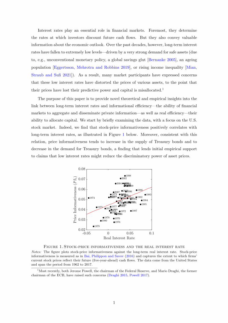
ability to allocate capital. We start by briefly examining the data, with a focus on the U.S.
stock market. Indeed, we find that stock-price informativeness positively correlates with
long-term interest rates, as illustrated in Figure 1 below. Moreover, consistent with this
relation, price informativeness tends to increase in the supply of Treasury bonds and to
decrease in the demand for Treasury bonds, a finding that lends initial empirical support
to claims that low interest rates might reduce the discriminatory power of asset prices.
Figure 1. Stock-price informativeness and the real interest rateNotes: The figure plots stock-price informativeness against the long-term real interest rate. Stock-priceinformativeness is measured as in Bai, Philippon and Savov (2016) and captures the extent to which firms’current stock prices reflect their future (five-year-ahead) cash flows. The data come from the United Statesand span the period from 1962 to 2017.
1Most recently, both Jerome Powell, the chairman of the Federal Reserve, and Mario Draghi, the formerchairman of the ECB, have raised such concerns (Draghi 2015, Powell 2017).
1

The remainder of the paper is dedicated to understanding the theoretical underpinnings
of these empirical patterns. For that purpose, we develop a novel noisy rational expectations
equilibrium (REE) model of the stock market. The model differs from traditional REE
models, such as those of Grossman and Stiglitz (1980) and Hellwig (1980), along one key
dimension: we relax the traditional assumption that the bond is in perfectly elastic supply,
with the interest rate given exogenously (which rules out any learning from the interest rate).
Instead, we assume that the bond is imperfectly elastic (e.g., fixed). As a consequence, the
equilibrium interest rate now plays a dual role: it determines the discount rate and reveals
information to investors.
Formally, this change manifests in the following three features that distinguish our
model from other REE models of the stock market. First, the interest rate is endogenously
determined. Second, investors learn not only from their private signals and the stock price
but also from the interest rate. Third, investors make intertemporal consumption choices.
Otherwise, the model is kept parsimonious to illustrate the economic mechanisms in the
clearest possible way. That is, we consider a two-period model with a continuum of risk-
averse investors who receive private signals about the fundamental. They trade a risk-free
bond and a risky stock in competitive markets. Noise traders operating in both the stock and
the bond market, prevent asset prices from being perfectly revealing. Finally, to illustrate
the implications for allocative efficiency, we endogenize output and explicitly model the
investment decision of the firm underlying the stock.
Primarily, we use the model to study how and what type of information investors learn
from the bond market. Our key finding can be summarized as follows: The interest rate (or,
more precisely, the resultant bond-market signal) reveals information about noise traders’
demand in the stock market that, in turn, allows investors to extract more precise infor-
mation about fundamentals from stock prices. Put differently, the bond market conveys
information about discount rates that, in turn, makes stock prices more informative about
cash flows.2
The intuition simply derives from budget constraints and market clearing; accordingly,
assume first that investors only consume at the terminal date.3 Investors’ budget constraints
then imply that their aggregate bond and stock expenditures add up to their aggregate ini-
2In line with the literature, we interpret noise-trader shocks as discount rate news because these shocksaffect (expected) returns without affecting fundamentals.
3In this case, we are able to characterize the equilibrium in closed form, even though prices are nonlinearfunctions of the state variables. In contrast, the model with intertemporal consumption choices does notyield an analytical solution and is solved numerically.
2

tial wealth (i.e., the economy’s aggregate-resource constraint). In addition, market clearing
in the stock market requires that investors’ aggregate stock demand equals the stock supply
minus noise traders’ demand. Consequently, conditional on prices and aggregate wealth,
any changes in noise traders’ stock demand must be accommodated (accompanied?) by
changes in investors’ aggregate bond demand. Under the traditional assumption of a bond
in perfectly elastic supply, such changes in aggregate bond demand do not affect the interest
rate; quantities, not prices, adjust. In contrast, with a imperfectly elastic fixed (e.g., fixed)
bond supply, the interest rate adjusts. As a result, the bond market (through the rate of
interest) provides a signal that allows investors to learn about noise traders’ stock demand,
with the signal error originating from noise traders’ bond demand.
The economic intuition extends to more complex settings, such as when investors con-
sume early, trade multiple risky assets, or hold money or when aggregate wealth is stochastic.
For instance, allowing for intertemporal consumption choices adds noise to the bond-market
signal, but leaves the basic inference problem unchanged.
Notably, our model further implies that the precision of the bond-market signal generally
increases in the rate of interest. Intuitively, because the signal stems from the aggregate-
resource constraint in the economy, noise traders’ bond demand enters the signal through
their bond expenditures, that is, divided by the rate of interest. As such, a higher interest
rate generally attenuates the noise in the bond-market signal and, hence, the precision of
the signal increases in the interest rate.4 Put differently, a higher interest rate makes the
bond-market-clearing condition less sensitive to variations in noise traders’ bond demand
(while keeping fixed its sensitivity to noise traders’ stock demand); hence, the signal-to-noise
ratio improves. A more precise bond market signal, in turn, allows investors to extract more
information about fundamentals from stock prices and results in stock-price informativeness
increasing in the interest rate.
After establishing the economic mechanism through which investors learn from the in-
terest rate, we use our model to discuss how variations in the bond supply (or, equivalently,
in the bond demand) affect informational and allocative efficiency as well as equilibrium
4To be precise, this property requires the stochastic component of noise traders’ bond demand havea price-elasticity below unity. If this isn’t the case, then an increase in the interest rate might lead toan increase in noise traders’ bond demand large enough to offset the attenuating effect of dividing by theinterest rate, leading to a rise in their bond expenditures. This case is however largely inconsistent with ourtheoretical and empirical findings. Indeed, we find, when endogenizing noise traders’ bond demand (SectionII), that price-inelastic shocks emerge naturally—as stipulated in, e.g., preferred-habitat theories of the termstructure. Moreover, we demonstrate that adding unit-elasticity shocks (which are also a natural outcome)do not overturn the noise-dampening effect of high interest rates. Finally, our empirical finding of a positiverelationship between stock price informativeness and bond supply also points to a low elasticity.
3

asset prices. Our main results can be summarized as follows. First, because the interest rate
increases in the bond supply, stock-price informativeness also increases in the bond supply
(or, conversely, declines with bond demand), an effect that can be entirely attributed to
learning from the bond-market signal. Second, the higher stock-price informativeness allows
the firm to better differentiate between high-productivity and low-productivity states and,
hence, to make more efficient investment decisions. Consequently, allocative efficiency in
the economy also increases in the bond supply. Third, because of a decline in risk (thanks to
higher stock-price informativeness), the bond supply negatively correlates with the stock’s
expected excess return and return volatility.
We also consider two extensions of our main framework featuring additional signals.
Both not only confirm the main economic mechanism but also deliver new insights. The
first extension, which allows for multiple risky assets, shows that the bond-market signal
induces a negative correlation between stocks’ excess returns (which declines in the bond
supply), despite fundamentals and noise trading being independent across the two stocks.
The second extension, which includes money, demonstrates that, similar to the rate of
interest, the rate of inflation provides information about noise traders’ stock demand (i.e.,
discount rate news). Moreover, the precision of the money market signal is increasing
in the rate of inflation, and, thus, a larger money supply leads to improved stock-price
informativeness and improved allocative efficiency.
Overall, these results highlight that the supply of (and demand for) bonds has important
implications for price informativeness, allocative efficiency, output, and asset prices. In
particular, variations in the bond supply influence the stock market and the real economy
not only through their traditional impact on discount rates but also through their impact
on the information environment. Indeed, these findings support critics who argue that, by
purchasing government bonds through QE programs, central banks degrade informational
and allocative efficiency.5
Our theoretical analyses also generate a rich set of novel predictions that are consistent
with broad features of the data. For instance, our model predicts that stock-price informa-
tiveness increases in the real interest rate (and in bond and money supplies), in line with
5For example, in July 2018, the former chairman of the Federal Reserve, Ben Bernanke, warned that,because of QE-induced “distortions” in financial markets, a yield curve inversion need not point to a recession.Similar claims have been made about the effect of asset-purchase programmes by the European Central Bankand the Bank of Japan. Moreover, worries that low interest rates might distort stock prices and lead toa misallocation of capital have been frequently voiced, for instance by Richard Fisher, head of the FederalReserve Bank of Dallas, Mario Draghi, then chairman of the ECB, and Jerome Powell, the chairman of theFederal Reserve (Fisher 2013, Draghi 2015, Powell 2017).
4

our empirical investigation. Related, the model predicts that allocative efficiency should
be high (low) in high (low) interest-rate environments. This prediction is consistent with
the empirical evidence presented by Gopinath et al. (2017), who document a simultaneous
decline in the real interest rate and capital allocation efficiency in southern European coun-
tries. Moreover, in the model, periods of low interest rates are associated with an increase
in the market price of risk, in the mean and variance of excess returns, and in stock-return
comovement. Combined with the cyclicality of interest rates observed in the data, these
results imply that the level and price of risk, as well as the volatility and comovement of
stock returns, are all countercyclical, as in the data. More work is needed to ascertain
whether these associations are actually causal or mere correlations.
The paper spans several strands of the literature. First and foremost, it builds on the
extensive noisy REE literature pioneered by Grossman and Stiglitz (1980) and Hellwig
(1980). Our main contribution to this literature is to endogenize the rate of interest. We
show that the interest rate contains valuable information about a stock’s noisy demand (or,
equivalently, supply) and work out how investors use this information to update their beliefs
about a stock’s payoff. We are not aware of any other work in which both stock prices and
the interest rate reveal information.6 That price informativeness and investors’ posterior
precision endogenously vary with the rate of interest and, hence, with the business cycle
further distinguishes our model from other noisy REE models. Likewise, this property con-
nects our work to that of Kacperczyk, van Nieuwerburgh and Veldkamp (2016), who analyze
how investors’ knowledge depends on the state of the economy. But the mechanism they
highlight is markedly different from ours in that this dependence on the state of the econ-
omy stems from variations in risk and in the price of risk (Kacperczyk, van Nieuwerburgh
and Veldkamp 2016) versus variations in the interest rate (our model).
Our paper further relates to three substreams of the noisy REE literature. The first
studies economies with multiple assets (see, e.g., Admati (1985), Brennan and Cao (1997),
Kodres and Pritsker (2002), van Nieuwerburgh and Veldkamp (2009, 2010), Biais, Bossaerts
and Spatt (2010), Kacperczyk, van Nieuwerburgh and Veldkamp (2016)). Though our main
model features two assets with informative prices, it distinctly differs from these models in
that our second asset is risk-free. In particular, we show that the risk-free asset reveals
6Detemple (2002) also proposes an REE model in which the interest rate is endogenous. However, in hissetting, information is revealed only through the interest rate (whereas the stock price does not reveal anyinformation), and, moreover, this information pertains to cash flows. Indeed, the economic mechanism andinsights differ substantially; for example, the (positive) link that we highlight between the interest rate andstock-price informativeness is absent from his framework.
5

information about the stock despite its payoff and noisy demand being uncorrelated with
those of the stock. This is in sharp contrast to Admati (1985) and the work that followed,
in which, absent (exogenous) cross-asset correlations, nothing is to be learned from one
asset about another. In addition, in our extension to multiple stocks, bond market clearing
endogenously generates a (negative) correlation between stocks’ returns (which is also absent
in Admati 1985). Second, through its emphasis on information about the stock’s noisy
demand (or, equivalently, its supply), our work is also related to Watanabe (2008), Ganguli
and Yang (2009), Manzano and Vives (2011), Farboodi and Veldkamp (2019), and Yang
and Zhu (2019). In these papers, investors receive a private and exogenous signal (which
they either purchase or are endowed with) about the stock supply. In contrast, the supply
signal (also referred to as order flow or discount rate information in the literature) is public
and endogenous in our setup. Finally, our paper is part of the substream of the literature
that seeks to generalize noisy REE models and explore their robustness to assumptions (see,
e.g., Barlevy and Veronesi 2000, 2003, Peress 2004, Breon-Drish 2015, Banerjee and Green
2015, Albagli, Hellwig and Tsyvinski 2015). Our contribution is to endogenize the interest
rate in an otherwise standard noisy REE model and identify what features survive or differ.
Our work also relates to the literature studying the impact of monetary policies on stock
prices.7 While this literature typically assumes information is symmetric across investors,
we allow for private (asymmetric) information. Doing so makes it possible to analyze the
impact of monetary policy on the informational and allocative efficiency of the stock market.
Related, a large literature in macroeconomics studies the impact of financial frictions, in
particular, credit constraints, on capital misallocation and real efficiency.8 In contrast, the
friction we consider (asymmetric information) operates in the stock market.
Finally, our paper relates to the literature studying the importance of an endogenous
rate of interest in asset pricing models under symmetric information. Lowenstein and
Willard (2006) highlight that, the assumption of the riskless asset being in perfectly elastic
supply can yield misleading conclusions (e.g., with respect to the impact of noise traders or
violations of the Law of One Price). Our work is distinctly different from their paper because
of the presence of private information and our focus on price informativeness. Moreover,
7Lucas (1982), LeRoy (1984a,b), Svensson (1985), Danthine and Donaldson (1986), and Marshall (1992)study how changes in monetary policy affect real and nominal asset prices. Sellin (2001) surveys this topic.
8See, for example, Bernanke and Gertler (1989) or Kiyotaki and Moore (1997). Brunnermeier andPedersen (2008), Rampini and Viswanathan (2010), He and Krishnamurthy (2013), Biais, Hombert andWeill (2014), and Brunnermeier and Sannikov (2014), among others, study the impact of frictions on assetprices.
6
we find that the main conclusions of the traditional noisy REE literature are robust to
endogenizing the interest rate. Instead, we illustrate that new (unexplored) mechanisms
arise when the bond market clears under a fixed bond supply.
The remainder of the paper is organized as follows. Section I presents the novel empir-
ical findings motivating our theoretical analysis. Section II introduces our main economic
framework. Section III discusses, in a tractable version of the model, the economic mech-
anism through which investors learn from the interest rate. In Section IV, we then study
the full model and relate the characteristics of the bond market to equilibrium outcomes.
Section V explores extensions with additional price signals. Finally, Section VI concludes.
The appendix provides the proofs and describes the numerical solution approach.
I. Empirical Patterns in Price Informativeness
In this section, we offer novel empirical evidence on the relation between the informativeness
of stock prices and characteristics of the bond market. In particular, we document patterns
in price informativeness linked to long-term interest rates and to the supply of and the
demand for Treasury bonds that guide the theory presented in the next sections.
I.A. Data and Estimation Procedures
Our analysis focuses on the U.S. market over the period from 1962 to 2017.
Price Informativeness: We measure the informativeness of stock prices using the proxy
developed by Bai, Philippon and Savov (2016). Their proxy captures the extent to which
firms’ current stock prices reflect their future cash flows and directly relates to capital
allocation efficiency. Specifically, in each year, we run the following cross-sectional regression
of year-t+h earnings on year-t stock prices:
Ej,t+hAj,t
= at,h + bt,h log
(Mj,t
Aj,t
)+ ct,hXj,t + εj,t,h, (1)
where h denotes the forecasting horizon; Ej,t+h/Aj,t denotes firm j’s earnings before interest
and taxes (EBIT) in year t+h scaled by year-t total assets; Mj,t/Aj,t denotes firm j’s market
capitalization (i.e., stock price times the number of shares outstanding) in year t scaled by
7

year-t total assets; and Xj,t denotes a set of firm-level controls, namely, current earnings,
Ej,t/Aj,t, and industry fixed effects (one-digit SIC codes).9
Intuitively, the coefficient bt,h reflects how closely current stock prices track future earn-
ings and, hence, how much fundamental information is capitalized in stock prices. Price
informativeness at horizon h, PIt,h, is then measured as the coefficient estimate bt,h multi-
plied by the year-t cross-sectional standard deviation of (scaled) stock prices:
PIt,h = bt,h × σt
(log
(Mj,t
Aj,t
)). (2)
As discussed in Bai, Philippon and Savov (2016), PI2t,h captures the variance of the pre-
dictable component of firms’ payoffs, Fj , given stock prices: Var(E[Fj |Pj ]). Hence, PIt,h
serves as a natural proxy for forecasting price efficiency.
We obtain stock price data from the Center for Research in Security Prices (CRSP) and
accounting data from Compustat. Like Bai, Philippon and Savov (2016), we focus on S&P
500 nonfinancial firms whose characteristics have remained remarkably stable over time.10
Moreover, we concentrate on forecasting horizons (h) of 3 and 5 years, horizons that, from a
capital allocation perspective, are most important (see, e.g., the time-to-build literature, in
particular, Koeva 2000) and for which prices are particularly useful in predicting earnings
(as reported in Bai, Philippon and Savov 2016).
Bond Market Characteristics: Our measures of bond market characteristics closely fol-
low those used by Krishnamurthy and Vissing-Jorgensen (2012). U.S. real interest rates are
obtained by deducting expected inflation from long-term nominal rates. The nominal rate
on long-maturity Treasury bonds is measured as the average yield on government bonds
with a maturity of 10 years or longer (up to 1999) and the 20-year Treasury constant-
maturity rate (from 2000 on), both of which are obtained from the Federal Reserve’s FRED
9To align price informativeness with bond market characteristics, we sample stock prices at the end of theU.S. government’s fiscal year (either June or September). For each firm, we measure accounting variables atthe end of the previous fiscal year—typically December—to ensure that the information is readily available tomarket participants. We adjust earnings using the gross domestic product (GDP) deflator from the Bureauof Economic Analysis (BEA).
10In contrast, as shown in Bai, Philippon and Savov (2016), the characteristics of non-S&P-500 firmshave dramatically changed over time, rendering any time-series analysis potentially misleading.
8
database. Expected inflation is estimated using a simple random-walk model (applied to
the Consumer Price Index of the BEA).11
To measure the supply of U.S. Treasuries, we use the U.S. government debt-to-GDP
ratio, specifically the ratio of the market value of publicly held government debt to GDP.
For that purpose, we adjust the book (par) value of U.S. government debt (obtained from
the Treasury Bulletin) using the Treasury debt market price index provided by the Dallas
Fed. Government debt and, accordingly, GDP are measured at the end of the government’s
fiscal year (i.e., the end of June up to 1976 and the end of September from 1977 onward).12
To explicitly study the impact of demand-driven factors, such as quantitative easing, we
also include in our analysis the Federal Reserve banks’ holdings of U.S. Treasury securities
and, as an instrument, their holdings of mortgage-backed securities (MBS). Both are scaled
by U.S. GDP and based on data from the Federal Reserve System.
Control Variables: We estimate stock market and cash flow volatility as the annualized
standard deviation of daily S&P 500 returns over the past 12 months and the cross-sectional
standard deviation of firms’ (scaled) earnings, respectively.
Table A1 in Appendix A reports summary statistics for all variables.
I.B. Price Informativeness and Bond Market Characteristics
In the first step, we analyze the relation between the informativeness of stock prices and
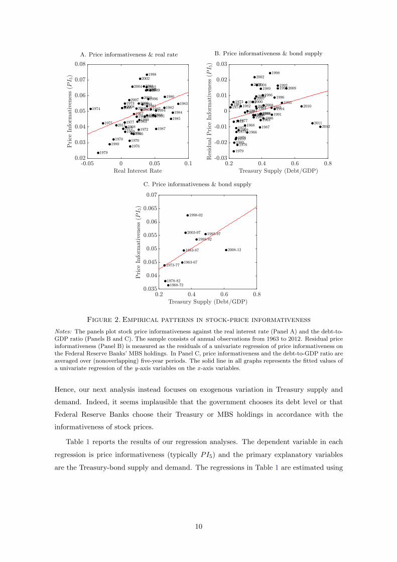
the real interest rate. Panel A of Figure 2, which plots five-year price informativeness,
PI5, against the real interest rate, strongly suggests a positive correlation between the
two series.13 A corresponding regression of price informativeness on the real interest rate
confirms that this positive relation is statistically significant, with a slope coefficient of
0.179 (t-statistic of 2.67). In terms of economic magnitude, a one-standard-deviation (SD)
increase in the real interest rate leads to a 0.42-SD increase in price informativeness.
A natural limitation of this test is that the rate of interest is endogenous; that is, it
is determined in equilibrium jointly with other quantities, including price informativeness.
11The random-walk model delivers the best out-of-sample performance for predicting inflation over oursample period. Our findings are robust to the use of alternative models for expected inflation, namely, AR(1)and ARMA(1,1) models.
12Our results remain unchanged when using the debt-to-GDP series prepared by Krishnamurthy andVissing-Jorgensen (2012). In fact, the correlation between the two data series is 0.9966. We are grateful tothe authors for sharing their data with us.
13Our time series of price informativeness ends in 2012, because we need to forecast five-year-aheadearnings, which go until 2017.
9
A. Price informativeness & real rate B. Price informativeness & bond supply
C. Price informativeness & bond supply
Figure 2. Empirical patterns in stock-price informativeness
Notes: The panels plot stock price informativeness against the real interest rate (Panel A) and the debt-to-GDP ratio (Panels B and C). The sample consists of annual observations from 1963 to 2012. Residual priceinformativeness (Panel B) is measured as the residuals of a univariate regression of price informativeness onthe Federal Reserve Banks’ MBS holdings. In Panel C, price informativeness and the debt-to-GDP ratio areaveraged over (nonoverlapping) five-year periods. The solid line in all graphs represents the fitted values ofa univariate regression of the y-axis variables on the x -axis variables.
Hence, our next analysis instead focuses on exogenous variation in Treasury supply and
demand. Indeed, it seems implausible that the government chooses its debt level or that
Federal Reserve Banks choose their Treasury or MBS holdings in accordance with the
informativeness of stock prices.
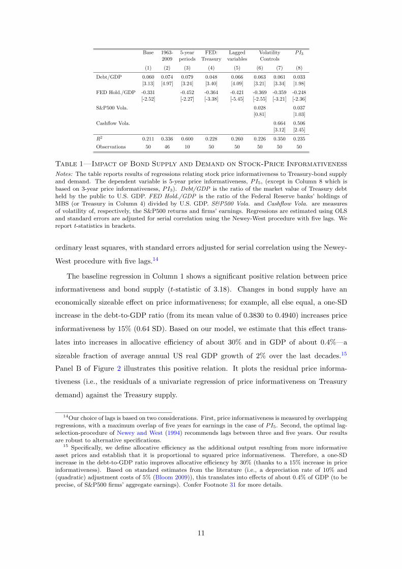
Table 1 reports the results of our regression analyses. The dependent variable in each
regression is price informativeness (typically PI5) and the primary explanatory variables
are the Treasury-bond supply and demand. The regressions in Table 1 are estimated using
10
Base 1963- 5-year FED: Lagged Volatility PI3
2009 periods Treasury variables Controls
(1) (2) (3) (4) (5) (6) (7) (8)
Debt/GDP 0.060 0.074 0.079 0.048 0.066 0.063 0.061 0.033[3.13] [4.97] [3.24] [3.40] [4.09] [3.21] [3.34] [1.98]
FED Hold./GDP -0.331 -0.452 -0.364 -0.421 -0.369 -0.359 -0.248[-2.52] [-2.27] [-3.38] [-5.45] [-2.55] [-3.21] [-2.36]
S&P500 Vola. 0.028 0.037[0.81] [1.03]
Cashflow Vola. 0.664 0.506[3.12] [2.45]
R2 0.211 0.336 0.600 0.228 0.260 0.226 0.350 0.235
Observations 50 46 10 50 50 50 50 50
Table 1—Impact of Bond Supply and Demand on Stock-Price Informativeness
Notes: The table reports results of regressions relating stock price informativeness to Treasury-bond supplyand demand. The dependent variable is 5-year price informativeness, PI5, (except in Column 8 which isbased on 3-year price informativeness, PI3). Debt/GDP is the ratio of the market value of Treasury debtheld by the public to U.S. GDP. FED Hold./GDP is the ratio of the Federal Reserve banks’ holdings ofMBS (or Treasury in Column 4) divided by U.S. GDP. S&P500 Vola. and Cashflow Vola. are measuresof volatility of, respectively, the S&P500 returns and firms’ earnings. Regressions are estimated using OLSand standard errors are adjusted for serial correlation using the Newey-West procedure with five lags. Wereport t-statistics in brackets.
ordinary least squares, with standard errors adjusted for serial correlation using the Newey-
West procedure with five lags.14
The baseline regression in Column 1 shows a significant positive relation between price
informativeness and bond supply (t-statistic of 3.18). Changes in bond supply have an
economically sizeable effect on price informativeness; for example, all else equal, a one-SD
increase in the debt-to-GDP ratio (from its mean value of 0.3830 to 0.4940) increases price
informativeness by 15% (0.64 SD). Based on our model, we estimate that this effect trans-
lates into increases in allocative efficiency of about 30% and in GDP of about 0.4%—a
sizeable fraction of average annual US real GDP growth of 2% over the last decades.15
Panel B of Figure 2 illustrates this positive relation. It plots the residual price informa-
tiveness (i.e., the residuals of a univariate regression of price informativeness on Treasury
demand) against the Treasury supply.
14Our choice of lags is based on two considerations. First, price informativeness is measured by overlappingregressions, with a maximum overlap of five years for earnings in the case of PI5. Second, the optimal lag-selection-procedure of Newey and West (1994) recommends lags between three and five years. Our resultsare robust to alternative specifications.
15 Specifically, we define allocative efficiency as the additional output resulting from more informativeasset prices and establish that it is proportional to squared price informativeness. Therefore, a one-SDincrease in the debt-to-GDP ratio improves allocative efficiency by 30% (thanks to a 15% increase in priceinformativeness). Based on standard estimates from the literature (i.e., a depreciation rate of 10% and(quadratic) adjustment costs of 5% (Bloom 2009)), this translates into effects of about 0.4% of GDP (to beprecise, of S&P500 firms’ aggregate earnings). Confer Footnote 31 for more details.
11

Consistent with a positive correlation between price informativeness and Treasury sup-
ply, Column 1 also documents a strong negative correlation between price informativeness
and bond demand, measured by the FED’s MBS holdings (t-statistic of −2.29). All else
equal, an increase in the FED’s MBS holdings from its mean of 0.005 to 0.06 (the mean
following QE) lowers price informativeness by more than 35%, or a 1.61 SD.
The remainder of Table 2 confirms that our findings hold up to a series of robustness
checks. Column 2 focuses on the period from 1962 to 2009, over which Treasury demand
was constant and so does not need to be controlled for.16 Column 3 (also illustrated in
Panel C) exploits only low-frequency variations in the series; that is, it reports the results
of a regression of (nonoverlapping) five-year averages of the variables (i.e., a total of 10 data
points). Column 4 uses the FED’s Treasury holdings (instead of their MBS holdings) to
control for Treasury demand. Column 5 lags bond supply and demand. Columns 6 and 7
control for stock market and cash flow volatility, respectively. Finally, Column 8 uses the
price-informativeness measure, PI3, based on a three-year forecasting horizon.
Taken together, the regressions in Table 1 provide robust empirical evidence that price
informativeness positively correlates with Treasury supply and negatively correlates with
Treasury demand. These results pose a substantial challenge to traditional information
choice models and motivate our subsequent theoretical analysis.
II. An REE Model with Bond Market Clearing
In this section, we introduce our main economic framework. The framework differs from
traditional competitive rational expectation equilibrium (REE) models, such as those of
Grossman and Stiglitz (1980), Hellwig (1980), and Verrecchia (1982), along three key (re-
lated) dimensions. First, the bond market clears, and the rate of interest is endogenously
determined. Second, investors learn not only from their private signals and the stock price
but also from the interest rate. Third, agents consume not only in the final period but also
in the trading period. Moreover, to illustrate the implications for allocative efficiency, we
endogenize firms’ real-investment decisions and, thus, output. In the following, we describe
the details of the model.
16Among others, Gorton, Lewellen and Metrick (2012) document that Treasury demand for “safe”(information-insensitive) debt was constant during this period.
12
t = 1 t = 2
Investors: Observe private signal,
stock price, and interest rate.
Set up portfolio and consume.
Firm (manager): Observes
stock price and interest rate.
Chooses real investment.
Bond and stock market: Clear.
Investors: Consumeproceeds from investments.
Firm: Productivity and
output are realized.
1
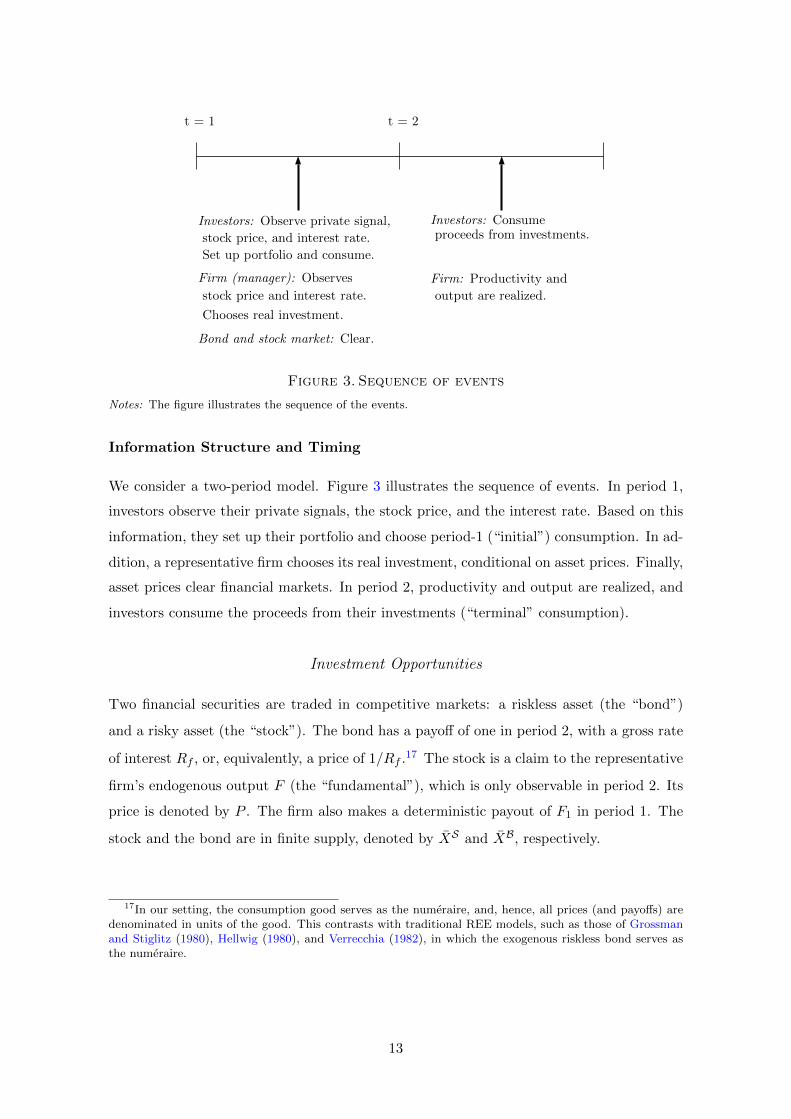
Figure 3. Sequence of events
Notes: The figure illustrates the sequence of the events.
Information Structure and Timing
We consider a two-period model. Figure 3 illustrates the sequence of events. In period 1,
investors observe their private signals, the stock price, and the interest rate. Based on this
information, they set up their portfolio and choose period-1 (“initial”) consumption. In ad-
dition, a representative firm chooses its real investment, conditional on asset prices. Finally,
asset prices clear financial markets. In period 2, productivity and output are realized, and
investors consume the proceeds from their investments (“terminal” consumption).
Investment Opportunities
Two financial securities are traded in competitive markets: a riskless asset (the “bond”)
and a risky asset (the “stock”). The bond has a payoff of one in period 2, with a gross rate
of interest Rf , or, equivalently, a price of 1/Rf .17 The stock is a claim to the representative
firm’s endogenous output F (the “fundamental”), which is only observable in period 2. Its
price is denoted by P . The firm also makes a deterministic payout of F1 in period 1. The
stock and the bond are in finite supply, denoted by XS and XB, respectively.
17In our setting, the consumption good serves as the numeraire, and, hence, all prices (and payoffs) aredenominated in units of the good. This contrasts with traditional REE models, such as those of Grossmanand Stiglitz (1980), Hellwig (1980), and Verrecchia (1982), in which the exogenous riskless bond serves asthe numeraire.
13

Output
Output is produced by a representative firm that employs a linear (“ZK”) production tech-
nology and is endowed with assets in place K1. Its fundamental value, v, is modeled as in
standard q-theory:
v(z, I) ≡ (K1 − I)︸ ︷︷ ︸≡F1
+ (1 + z)((1− δ)K1 + I
)− κ
2K1I2︸ ︷︷ ︸
≡F
. (3)
Specifically, with period-1 productivity being normalized to one, initial-period output, F1,
is simply given by assets-in-place K1 less investment I. Period-2 output, F , is given by
the product of period-2 productivity, 1 + z, and available capital (assets-in-place K1 de-
preciated at rate δ, plus investment I), minus quadratic adjustment costs (κ/2K1) I2 (with
κ ≥ 0).18 Period-2 net productivity, z, is random and normally distributed with mean zero
and precision τz: z ∼ N (0, 1/τz).
For simplicity, we assume that the firm (manager) has no private information about
productivity, z, but learns about productivity from stock and bond prices.19 This creates
a feedback effect from financial markets to real investment decisions.20
Investors
There exists a continuum of atomless investors with unit mass. At the beginning of period
1, each investor i receives a private signal about productivity: si = z + εi, where εi is i.i.d.
normally distributed with mean zero and precision τε. Investors have constant absolute risk
aversion (CARA) preferences over initial and terminal consumption, Ci,1 and Ci,2:
Ui(Ci,1, Ci,2) = −1
ρexp(−ρCi,1
)+ β E
[−1
ρexp(−ρCi,2
) ∣∣Fi] , (4)
18As is standard in such models, investment, I, can be positive (representing capital expenditures) ornegative (representing an asset sale).
19In particular, in our single-stock economy, the firm represents the entire productive sector, so z can beinterpreted as aggregate productivity, about which the manager has plausibly no private information.
20Bond, Edmans and Goldstein (2012) survey the literature on feedback effects. For more recent contri-butions, see Foucault and Fresard (2014), Edmans, Goldstein and Jiang (2015), Goldstein and Yang (2017),and Dessaint et al. (2018).
14

where ρ denotes absolute risk aversion; β ∈ (0, 1] denotes the rate of time preference; and
Fi = si, P,Rf describes investor i’s time-1 information set. Investors are each initially
endowed with Wi,1 units of the good (or, equivalently, of a maturing bond).21
Noise Traders
Noise (liquidity) traders operate in both the bond and the stock market. In particular, note
that, in addition to the usual stock market noise, we assume a noisy bond demand; this
assumption prevents the bond and stock prices from being jointly perfectly revealing.
Noise traders’ behavior is not explicitly modeled; instead, their demands are given by
exogenous random variables. Specifically, noise traders’ demand for the stock equals uS ∼N (0, 1/τuS ). Their demand for bonds equals uB1 + uB2 Rf , where uB1 ∼ N (0, 1/τuB1
) and
uB2 ∼ N (0, 1/τuB2). uB1 and uB2 , respectively, represent the price-inelastic and the price-
elastic components of bond noise. z, uS , uB1 , and uB2 are assumed uncorrelated.22
Equilibrium Definition
Investor i aims to maximize expected utility (4) subject to the following budget constraints:
Ci,1 +XSi P +XBi R−1f = Wi,1, and Ci,2 = XSi F +XBi , (5)
where XSi and XBi denote the number of shares of the stock and the bond held by the
investor, respectively. The objective of the manager is to maximize the expected firm value.
Accordingly, a rational expectations equilibrium is defined by consumption choices
Ci,1, Ci,2, portfolio choices XSi , XBi , a real investment choice I, and asset prices P,Rfsuch that
1. Ci,1, Ci,2 and XSi , XBi maximize investor i’s expected utility (4) subject to the
budget constraints in (5), taking prices P and Rf as given,
2. I maximizes the expected firm value E [v(z, I) |Rf , P ],
3. the investors’ and the manager’s expectations are rational,
21Endowing investors also with units of the stock does not affect the results (see Remark 1 in Ap-pendix B.A and Section IV.C).
22This correlation structure highlights that, in equilibrium, the bond price reveals information about thestock even though its payoff and demand are uncorrelated with those of the stock.
15

4. aggregate demand equals aggregate supply in the bond and the stock markets:23
∫ 1
0XSi di+ uS = XS , and
∫ 1
0XBi di+ uB1 + uB2 Rf = XB. (6)
It is important to highlight that, in equilibrium, both asset prices play a dual role: each price
not only clears its respective market but also aggregates and transmits investors’ private
information.
III. The Economic Mechanism
We now first illustrate how and what type of information investors learn from the interest
rate. To do so, we use a simplified version of our model that provides the key economic
intuition and allows for simple closed-form solutions. It deviates from the framework de-
scribed in the preceding section only in that investors consume exclusively on the terminal
date. Moreover, to facilitate the exposition of the economic mechanism, we abstract from
real investment and treat the stock’s payouts, F , as exogenous: F ∼ N (µF , 1/τF ). Hence,
the model essentially reduces to Hellwig’s (1980) but with bond market clearing.
III.A. Equilibrium
Because of learning from the interest rate, equilibrium asset prices are nonlinear functions of
the state variables—in stark contrast to traditional frameworks. However, by conjecturing
the functional form of the market-clearing conditions (which remain linear), instead of
stipulating the functional form of the interest rate and the stock price (which are not
linear), we are still able to characterize the equilibrium in closed form, as stated in the
following theorem:
23By Walras’ law, market clearing in the bond and the stock market guarantees market clearing in thegoods market in period 1.
16

Theorem 1. There exists a unique (conditionally linear) rational expectations equilibrium.
The equilibrium asset prices are characterized by
Rf =XB − uB1
W1 −(XS − uS
)P + uB2
; and (7)
Rf P =
(τFτµF +
τε τuS |sB
ρ τµuS |sB
)+τε
(ρ2 + τε τuS |sB
)τ ρ2
(F − ρ
τεuS), (8)
with τuS |sB , µuS |sB , and τ defined in Equations (13), (14), and (15) below (9)
and Wi ≡∫ 1
0Wi,1 di.
Investor i’s optimal stock and bond holdings equal
XSi =E[F | Fi]− P RfρVar(F | Fi)
and XBi = Rf(Wi,1 −XSi P
). (10)
The optimal demand for the stock, XSi , follows the standard mean-variance portfolio
rule. The optimal bond investment is simply given by initial wealth minus stock holdings.
The equilibrium interest rate, Rf , is a function of realized stock and bond demands and,
thus, is stochastic.24 As expected, it is increasing in the bond supply, XB, and declining in
the bond demand shocks uB1 and uB2 ; specifically, a larger residual supply requires a lower
bond price for the market to clear and, hence, a higher interest rate. Moreover, the interest
rate declines in investors’ aggregate wealth, W1, and increases in their stock expenditures,(XS − uS
)P .
The equilibrium price ratio, Rf P , has the familiar structure of, for example, that of
Hellwig (1980), with one critical difference: the ratio features the mean and precision of the
noisy stock demand, µuS |sB and τuS |sB , conditional on the interest rate, instead of its prior
mean and precision. This difference arises because investors use the information revealed
by the bond market to update their beliefs about the noise traders’ stock demand. In other
words, they receive discount rate news.
24 The gross interest rate, Rf , can be negative in this illustrative framework. This does not, however, leadto arbitrage opportunities. Indeed, negative rates are caused by the fact that investors have a preference overterminal consumption only (i.e., do not consume in period 1), and, thus, in contrast to our main economicframework analyzed in Section IV, the interest rate is entirely determined by budget considerations and notby marginal utilities.
17

Specifically, in the absence of initial consumption, investors’ period-1 budget constraints
and market clearing imply that values of the residual stock and bond supplies must sum up
to aggregate wealth, or, formally:(XS − uS
)P +
(XB − uB1 − uB2 Rf
)R−1f = W1 (11)
⇔ sB ≡ −Rf W1 − XS Rf P − XBRf P
= uS +uB1Rf P
+uB2P. (12)
Consequently, the bond market provides a signal, sB, about the (unobservable) stock de-
mand, uS , with the bond demands, uB1 and uB2 , acting as noise. The following lemma
describes the resultant conditional distribution of the noisy stock demand.
Lemma 1. The distribution of the noisy stock demand, uS , conditional on the bond-market
signal sB is characterized by
µuS |sB ≡ E[uS | sB
]=
1
τuS |sB
P 2
1R2f τuB1
+ 1τuB2
(−Rf W1 − XS RfP − XB
Rf P
); and (13)
τuS |sB ≡ Var(uS | sB
)−1= τuS +
P 2
1R2f τuB1
+ 1τuB2
. (14)
Intuitively, investors combine their prior beliefs with the signal provided by the bond
market to update their beliefs about the noisy stock demand. The conditional mean, µuS |sB ,
is simply the precision-weighted average of the prior mean (equal to zero) and the bond
signal in (12). Similarly, the conditional precision, τuS |sB , is the sum of the prior precision
(τuS ) and the precision of the bond market signal.
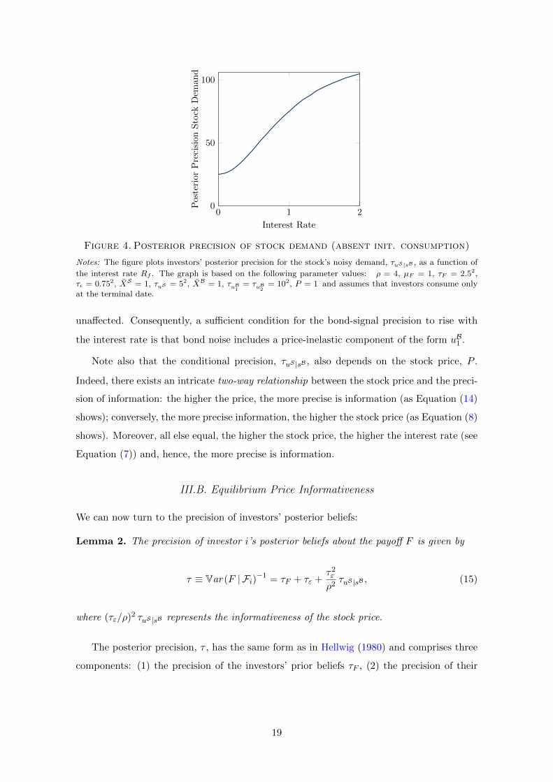
Notably, the conditional precision, τuS |sB , is increasing in the rate of interest Rf , as illus-
trated in Figure 4. Specifically, because the bond signal sB stems from investors’ aggregate-
resource constraint (11) (which ties together noise traders’ stock and bond demands), noise
traders’ bond demand enters the signal through their bond expenditures, that is, divided by
the rate of interest (see Equation (12)). Hence, a higher interest rate attenuates the signal’s
error and, thus, a more accurate signal of the stock’s demand.
Note that the positive link between the signal’s precision and the interest rate is driven
entirely by the price-inelastic component of noise, uB1 . Indeed, as Equation (12) illustrates,
only shocks to uB1 are attenuated by a higher rate of interest; in contrast, shocks to uB2 are
18
0 1 20
50
100
Interest Rate
PosteriorPrecisionStock
Dem
and
Figure 4. Posterior precision of stock demand (absent init. consumption)
Notes: The figure plots investors’ posterior precision for the stock’s noisy demand, τuS |sB , as a function of
the interest rate Rf . The graph is based on the following parameter values: ρ = 4, µF = 1, τF = 2.52,τε = 0.752, XS = 1, τuS = 52, XB = 1, τuB
1= τuB
2= 102, P = 1 and assumes that investors consume only
at the terminal date.
unaffected. Consequently, a sufficient condition for the bond-signal precision to rise with
the interest rate is that bond noise includes a price-inelastic component of the form uB1 .
Note also that the conditional precision, τuS |sB , also depends on the stock price, P .
Indeed, there exists an intricate two-way relationship between the stock price and the preci-
sion of information: the higher the price, the more precise is information (as Equation (14)
shows); conversely, the more precise information, the higher the stock price (as Equation (8)
shows). Moreover, all else equal, the higher the stock price, the higher the interest rate (see
Equation (7)) and, hence, the more precise is information.
III.B. Equilibrium Price Informativeness
We can now turn to the precision of investors’ posterior beliefs:
Lemma 2. The precision of investor i’s posterior beliefs about the payoff F is given by
τ ≡ Var (F | Fi)−1 = τF + τε +τ2ε
ρ2τuS |sB , (15)
where (τε/ρ)2 τuS |sB represents the informativeness of the stock price.
The posterior precision, τ , has the same form as in Hellwig (1980) and comprises three
components: (1) the precision of the investors’ prior beliefs τF , (2) the precision of their
19

private signal τε, and (3) the precision of the stock price signal (τε/ρ)2 τuS |sB , which is
driven by the precision of the stock demand τuS |sB and the signal-to-noise ratio of the stock
price signal (τε/ρ). Consistent with Hellwig (1980), the posterior precision is increasing
in all three precisions and in investors’ risk tolerance. However, as with the equilibrium
price function, price informativeness differs from the expression in Hellwig (1980) in that it
features investors’ precision of the stock demand conditional on the bond-market signal sB:
τuS |sB , rather than investors’ prior precision.
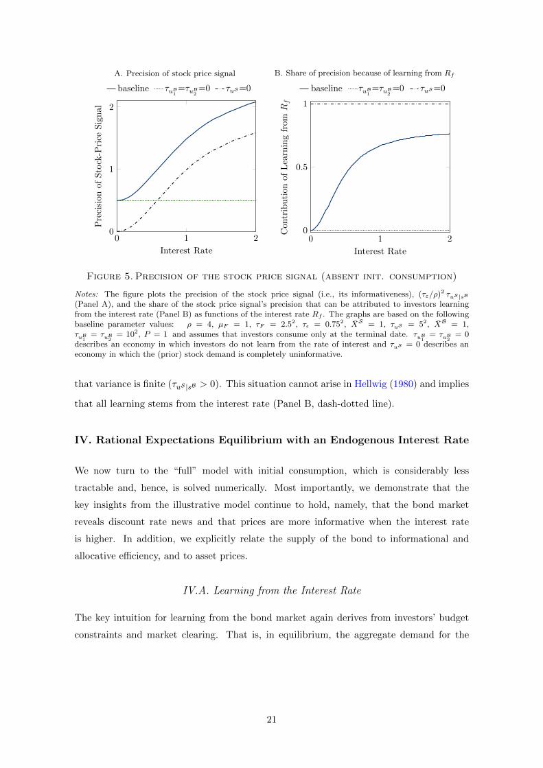
This observation has three important implications, which are illustrated in Panel A
of Figure 5, and which distinguish our model from traditional noisy REE models. First,
investors’ posterior precision is higher than in Hellwig (1980), thanks to the information
on the noisy stock demand obtained from the bond market. Second, price informativeness
depends on (specifically, increases in) the rate of interest, Rf , because a higher rate of
interest allows investors to extract more information from the stock’s price about its payoff
(thanks to their more precise information about the noisy stock demand). Accordingly,
the share of the stock price signal’s precision that can be attributed to learning from the
interest rate (relative to the overall precision of the stock price signal) increases in the rate
of interest (Panel B). Third, price informativeness and investors’ posterior precision are
stochastic and, hence, ex ante unknown—a feature that could, in a model with endogenous
information choice (in the spirit of Verrecchia 1982), deliver new insights into investors’
demand for information.
As is clear from (15), the impact of learning from the bond market signal is stronger,
the more precise the priors about the bond demand are (i.e., for a higher τuB1or τuB2
).
Accordingly, the share of the stock price signal’s precision that can be attributed to learning
from the interest rate also increases in the precision of the bond demand (not shown).
Figure 5 also illustrates two interesting limiting cases. First, if the variance of noise
trading in the bond market is infinite (τuB1= τuB2
= 0), then the precision of the stock signal
does not vary with the rate of interest (Panel A) because the bond signal cannot be used to
form more precise (conditional) beliefs about the stock’s demand; that is, τuS |sB = τuS .25
Accordingly, all learning can be attributed to the stock price (Panel B, dotted line). Second,
the stock signal provides information about the stock’s payoff even if the variance of noise
trading in the stock market is infinite (τuS = 0) because, conditional on the interest rate,
25As a result, the equilibrium price ratio, Rf P , coincides with that in Hellwig (1980). However, theinterest rate remains stochastic, so that the equilibrium is not identical to Hellwig’s.
20
A. Precision of stock price signal
0 1 20
1
2
Interest Rate
Precision
ofStock-P
rice
Signal
baseline τuB1=τuB
2=0 τuS=0
B. Share of precision because of learning from Rf
0 1 20
0.5
1
Interest Rate
Con
tributionofLearningfromR
f
baseline τuB1=τuB
2=0 τuS=0
Figure 5. Precision of the stock price signal (absent init. consumption)
Notes: The figure plots the precision of the stock price signal (i.e., its informativeness), (τε/ρ)2 τuS |sB
(Panel A), and the share of the stock price signal’s precision that can be attributed to investors learningfrom the interest rate (Panel B) as functions of the interest rate Rf . The graphs are based on the followingbaseline parameter values: ρ = 4, µF = 1, τF = 2.52, τε = 0.752, XS = 1, τuS = 52, XB = 1,τuB
1= τuB
2= 102, P = 1 and assumes that investors consume only at the terminal date. τuB
1= τuB
2= 0
describes an economy in which investors do not learn from the rate of interest and τuS = 0 describes aneconomy in which the (prior) stock demand is completely uninformative.
that variance is finite (τuS |sB > 0). This situation cannot arise in Hellwig (1980) and implies
that all learning stems from the interest rate (Panel B, dash-dotted line).
IV. Rational Expectations Equilibrium with an Endogenous Interest Rate
We now turn to the “full” model with initial consumption, which is considerably less
tractable and, hence, is solved numerically. Most importantly, we demonstrate that the
key insights from the illustrative model continue to hold, namely, that the bond market
reveals discount rate news and that prices are more informative when the interest rate
is higher. In addition, we explicitly relate the supply of the bond to informational and
allocative efficiency, and to asset prices.
IV.A. Learning from the Interest Rate
The key intuition for learning from the bond market again derives from investors’ budget
constraints and market clearing. That is, in equilibrium, the aggregate demand for the
21

stock and the bond plus aggregate consumption must equal aggregate wealth, or, formally:
(XS − uS
)P +
(XB − uB1 − uB2 Rf
)R−1f +
∫ 1
0Ci,1 di︸ ︷︷ ︸≡ C1
= W1
⇔ sB ≡ −Rf W1 − XS Rf P − XBRf P
= uS +uB1Rf P
+uB2P− C1
P. (16)
Hence, as in our illustrative framework in Section III, the bond market provides a signal, sB,
about the noisy stock demand uS (i.e., discount rate news), which, in turn, allows investors
to more precisely infer the fundamental. Note, however, that the signal is now perturbed not
only by noise traders’ bond demands (uB1 and uB2 ) but also by investors’ period-1 aggregate
consumption C1 (which is a function of the state variables and, hence, stochastic).
Note also that, because of investors’ intertemporal consumption choices, aggregate con-
sumption, C1, depends on expected trading profits, which are a nonlinear function of the
state variables.26 As a result, the bond-market-clearing condition (16) is no longer linear in
the state variables. Accordingly, the model must be solved numerically. For that purpose,
we extend the numerical solution approach presented in Breugem and Buss (2019) to allow
for learning from the interest rate, intertemporal consumption choices, and endogenous out-
put. The algorithm relies on discretizing the state space, which, in turn, allows to explicitly
compute investors’ posterior beliefs and to exactly solve the first-order and market-clearing
conditions. Notably, the algorithm allows for arbitrary price and demand functions; that
is, one does not need to parameterize these functions in any form. See Appendix C for
additional details.
In the following, we rely on a specific set of parameter values (displayed in the figure
captions) to illustrate the predictions of our model. We have confirmed that the patterns
exhibited in the figures obtain for a wide range of parameter values. Indeed, in all our
numerical analyses, the effect of variations in bond supply on informational and allocative
efficiency and asset prices is as illustrated below. At the end of the section, we provide a
brief comparative statics analysis to illustrate how the effects vary quantitatively with the
main parameters.
We confirm that the results of Section III continue to hold when investors consume early.
Namely, the bond market reveals information to investors and its precision increases in the
26In particular, expected trading profits typically depend on the aggregate squared Sharpe ratio,∫(E [F | Fi]−RfP )2 di, which is a nonlinear function of the state variables.
22

1 1.25 1.5
1.5
2
2.5
3
Interest Rate
Precision
ofStock-P
rice
Signal
low P high P
Figure 6. Precision of the Stock Price Signal
Notes: The figure plots the precision of the stock price signal as a function of the interest rate, Rf—for two levels of the stock price P . The precision of the stock price signal is measured as the differencebetween an (uninformed) investor’s posterior precision, conditional on public prices, and her prior precision:Var(z|P,Rf )−1 − τz. The graph is based on the following parameter values: β = 0.95, ρ = 4, τz = 2.52,τε = 0.752, XS = 1, τuS = 52, XB = 1, τuB
1= τuB
2= 102, Wi,1 = 3, K1 = 1, κ = 5, and δ = 0.
interest rate. Figure 6 illustrates this property (comparable to Panel A of Figure 5 from
the illustrative model). The mechanism is again that a higher interest rate attenuates the
noise originating from the stochastic bond demand , uB1 (whereas the bond noise uB2 remains
unaffected); as Equation (16) shows. Specifically, the attenuating effect of the interest rate
is not offset by any effect it might have on noise originating from aggregate consumption
C1. Figure 6 also shows that the stock price continues to play a similar attenuating role.
IV.B. Bond Supply, Informational Efficiency, and Asset Prices
We now study how variations in the bond supply affect informational and allocative ef-
ficiency and asset prices. Intuitively, variations in the bond supply (or demand) can be
linked to government and central bank policies through their influence on the level of the
bond supply/demand as well as its precision. For instance, an elevated bond demand due to
quantitative easing would lower the (residual) supply of bonds available to investors. Like-
wise, policies designed to stabilize long-term interest rates (e.g., by offsetting fluctuations in
23
A. Price informativeness
0.19
0.2
0.21Price
Inform
ativeness
baseline high τuB τuB=0
0.75 1 1.25
0.11
Bond Supply
B. Price ratio
0.56
0.58
0.6
Price
Ratio
baseline high τuB τuB=0
0.75 1 1.25
0.45
Bond Supply
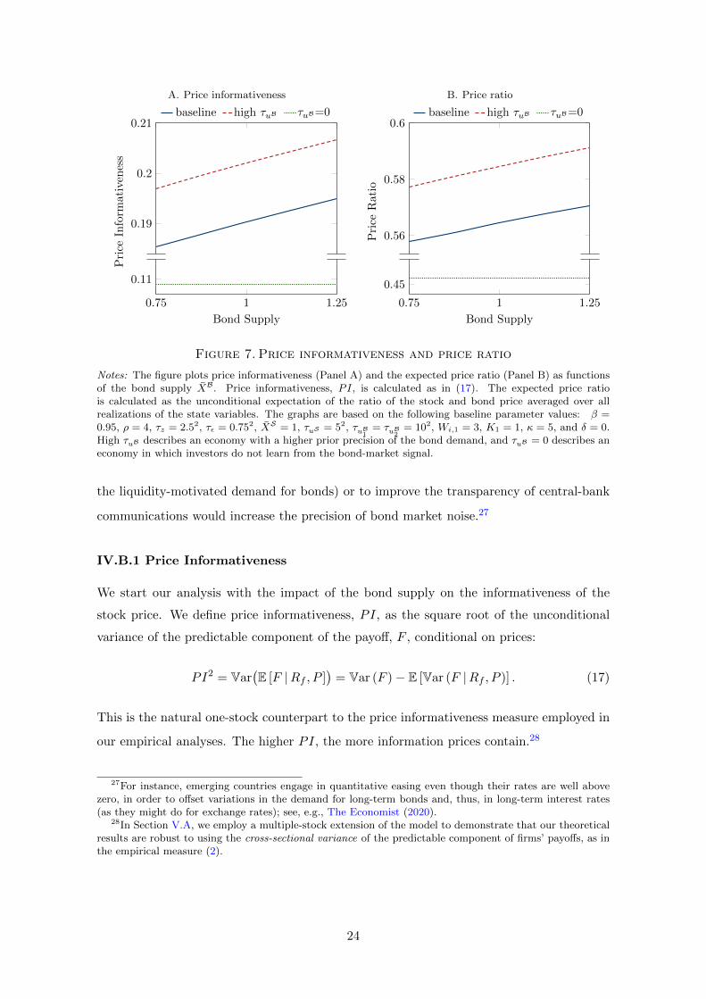
Figure 7. Price informativeness and price ratio
Notes: The figure plots price informativeness (Panel A) and the expected price ratio (Panel B) as functionsof the bond supply XB. Price informativeness, PI, is calculated as in (17). The expected price ratiois calculated as the unconditional expectation of the ratio of the stock and bond price averaged over allrealizations of the state variables. The graphs are based on the following baseline parameter values: β =0.95, ρ = 4, τz = 2.52, τε = 0.752, XS = 1, τuS = 52, τuB
1= τuB
2= 102, Wi,1 = 3, K1 = 1, κ = 5, and δ = 0.
High τuB describes an economy with a higher prior precision of the bond demand, and τuB = 0 describes aneconomy in which investors do not learn from the bond-market signal.
the liquidity-motivated demand for bonds) or to improve the transparency of central-bank
communications would increase the precision of bond market noise.27
IV.B.1 Price Informativeness
We start our analysis with the impact of the bond supply on the informativeness of the
stock price. We define price informativeness, PI, as the square root of the unconditional
variance of the predictable component of the payoff, F , conditional on prices:
PI2 = Var(E [F |Rf , P ]
)= Var (F )− E [Var (F |Rf , P )] . (17)
This is the natural one-stock counterpart to the price informativeness measure employed in
our empirical analyses. The higher PI, the more information prices contain.28
27For instance, emerging countries engage in quantitative easing even though their rates are well abovezero, in order to offset variations in the demand for long-term bonds and, thus, in long-term interest rates(as they might do for exchange rates); see, e.g., The Economist (2020).
28In Section V.A, we employ a multiple-stock extension of the model to demonstrate that our theoreticalresults are robust to using the cross-sectional variance of the predictable component of firms’ payoffs, as inthe empirical measure (2).
24
As Figure 7 illustrates, both stock-price informativeness and the price ratio, RfP , are
increasing in the bond supply, XB. Indeed, they reinforce each other in equilibrium: the
higher the price ratio, the more precise is information; conversely, the more precise infor-
mation, the higher is the price ratio. Specifically, an increase in the interest rate leads to an
increase in the price ratio, RfP , regardless of whether information is private. In our setup,
this increase improves the signal-to-noise ratio of the bond market signal (as discussed in
the preceding section) and, thus, stock-price informativeness.29 In turn, this improvement,
by reducing risk and the associated stock price discount, pushes up the stock price and,
hence, the price ratio. This leads to a further improvement in informativeness, generating
the concomitant increases in price informativeness and the price ratio (in the bond supply)
illustrated in Figure 7.30
As before, an increase in the prior precision of any of the bond-demand stocks, τuB1and
τuB2, improves the precision of the bond signal and, hence, strengthens its impact. Thus,
price informativeness and the price ratio go up further (Panels A and B). Only if the variance
of the noisy bond demands is infinite (τuB1= τuB2
= 0), is there no learning from the bond
(as in traditional REE models, such as Hellwig’ (1980)).
IV.B.2 Real Investment and Allocative Efficiency
The firm’s optimal investment, I, is characterized by the standard q-theory investment
condition (Tobin 1969):
I
K1=
E [z |P,Rf ]
κ. (18)
Importantly, the investment rate, I/K1, is driven by the manager’s conditional expec-
tation of productivity z, given asset prices. This creates a feedback from financial markets
to real investment decisions whereby the stock’s price (aggregating investors’ private infor-
mation) not only reflects but also affects the firm’s value. A natural measure of allocative
efficiency is the “surplus output” that is expected in excess of the output produced by an
29Our numerical analyses show that any noise originating from aggregate consumption only plays asecondary role here. Indeed, this increase in price informativeness in the supply of the bond shows up in allparametrizations of the model that we explore.
30Appendix B.A explicitly describes this two-way relation between the signal precision and the priceratio (which manifests itself in a cubic equation for the price ratio) in the illustrative model with arbitraryendowments. It demonstrates that stock-price informativeness is unambiguously increasing in the price ratio.
25

uninformed manager (who optimally invests zero):31
E = E[E [v(z, I) |P,Rf ]
]− E [v(z, 0)] . (19)
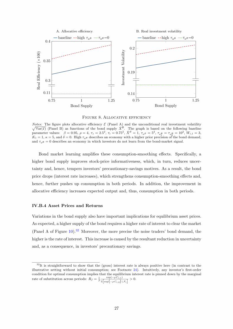
Panel A of Figure 8 shows that allocative efficiency is increasing in the bond supply.
Intuitively, the more precise the manager’s information, the more efficient the firm’s invest-
ment. In particular, the increase in stock-price informativeness (thanks to a larger bond
supply) allows the manager to improve her forecast of the productivity shock z and, hence,
her investment. Notably, the higher allocative efficiency does not result from a higher level
of investment. Instead, the positive effect of the bond supply on allocative efficiency re-
sults from more efficient investment decisions; that is, the manager can better differentiate
between high-productivity states (in which she should invest more) and low-productivity
states (in which she should invest less). The effect also manifests in a higher volatility of real
investment, as illustrated in Panel B. Again, the effects are stronger, the more informative
the bond demand (update notation high τuB).
IV.B.3 Consumption Choices
Variations in the bond supply also affect investors’ consumption choices, as Figure 9 illus-
trates. Multiple effects shape those choices.
First, standard consumption-smoothing effects (unrelated to bond market learning) are
at play. On the one hand, a higher rate of interest increases the price of period-1 consump-
tion relative to period-2 consumption and, thus, shifts consumption from period 1 to period
2 (substitution effect). On the other hand, a higher interest rate makes investors “richer”
and increases consumption in both periods (income effect). Both effects push up consump-
tion in period 2 but operate in opposite directions for period-1 consumption. For usual
levels of (absolute) risk aversion, the income effect dominates, and, hence, consumption in
period 1 increases as well (as can be seen in Panel A in the case of an uninformative bond
demand: τuB1= τuB2
= 0).
31 Note that surplus output E is proportional to squared price informativeness: E = (K1/2κ)PI2. More-over, because output in the absence of learning is equal to (2 − δ)K1 (and, hence, unrelated to priceinformativeness), variations in allocative efficiency can be directly traced back to variations in price infor-mativeness: dE/E = 2 dPI/PI. Consequently, the implied change in output O ≡ E
[E [v(z, I) |P,Rf ]
]is
given by:dO
O=dEO
=EO
dEE =
E/E [v(z, 0)]
1 + E/E [v(z, 0)]
dEE with
EE [v(z, 0)]
=1
2κ (2− δ) PI2,
which supports the quantitative assessment in Footnote 15.
26
A. Allocative efficiency
0.3
0.35
0.4R
eal
Effi
cien
cy(×
100
)baseline high τuB τuB=0
0.75 1 1.25
0.11
Bond Supply
B. Real investment volatility
0.19
0.2
InvestmentVolatility
baseline high τuB τuB=0
0.75 1 1.25
0.14
Bond Supply
Figure 8.Allocative efficiency
Notes: The figure plots allocative efficiency E (Panel A) and the unconditional real investment volatility√Var(I) (Panel B) as functions of the bond supply XB. The graph is based on the following baseline
parameter values: β = 0.95, ρ = 4, τz = 2.52, τε = 0.752, XS = 1, τuS = 52, τuB1
= τuB2
= 102, Wi,1 = 3,K1 = 1, κ = 5, and δ = 0. High τuB describes an economy with a higher prior precision of the bond demand,and τuB = 0 describes an economy in which investors do not learn from the bond-market signal.
Bond market learning amplifies these consumption-smoothing effects. Specifically, a
higher bond supply improves stock-price informativeness, which, in turn, reduces uncer-
tainty and, hence, tempers investors’ precautionary-savings motives. As a result, the bond
price drops (interest rate increases), which strengthens consumption-smoothing effects and,
hence, further pushes up consumption in both periods. In addition, the improvement in
allocative efficiency increases expected output and, thus, consumption in both periods.
IV.B.4 Asset Prices and Returns
Variations in the bond supply also have important implications for equilibrium asset prices.
As expected, a higher supply of the bond requires a higher rate of interest to clear the market
(Panel A of Figure 10).32 Moreover, the more precise the noise traders’ bond demand, the
higher is the rate of interest. This increase is caused by the resultant reduction in uncertainty
and, as a consequence, in investors’ precautionary savings.
32It is straightforward to show that the (gross) interest rate is always positive here (in contrast to theillustrative setting without initial consumption; see Footnote 24). Intuitively, any investor’s first-ordercondition for optimal consumption implies that the equilibrium interest rate is pinned down by the marginal
rate of substitution across periods: Rf = 1β
exp(−ρCi,1)
E[exp(−ρCi,2
)| Fi
] > 0.
27

A. Initial consumption
0.75 1 1.25
1.6
1.7
1.8
1.9
Bond Supply
InitialCon
sumption
baseline high τuB τuB=0
B. Terminal consumption
0.75 1 1.25
1.8
2
2.2
Bond Supply
Terminal
Consumption
baseline high τuB τuB=0
Figure 9.Consumption
Notes: The figure plots initial consumption (Panel A) and terminal consumption (Panel B) as functions of thebond supply XB. We report the unconditional expectation for both quantities averaged over all realizationsof the state variables. The graphs are based on the following baseline parameter values: β = 0.95, ρ = 4,τz = 2.52, τε = 0.752, XS = 1, τuS = 52, τuB
1= τuB
2= 102, Wi,1 = 3, K1 = 1, κ = 5, and δ = 0. High τuB
describes an economy with a higher prior precision of the bond demand, and τuB = 0 describes an economyin which investors do not learn from the bond-market signal.
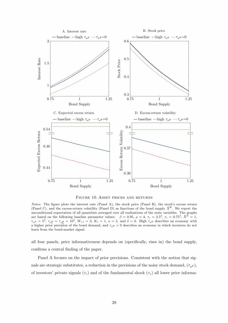
The stock price declines in the bond supply because of stronger discounting (Panel B).
Note, however, that the simultaneous improvement in price informativeness partially offsets
this decline as it reduces the risk borne by investors and, consequently, the price discount
they demand. By the same account, the stock’s expected excess return is decreasing in
the bond supply (Panel C). Finally, the increase in price informativeness also implies that
the stock’s price tracks its payoff more closely, thereby reducing the excess-return volatility
(Panel D). The latter two effects can be fully attributed to learning from the bond market
signal, as demonstrated by the comparison with the reference case of an uninformative bond
market (τuB1= τuB2
= 0). Accordingly, both effects are more pronounced for a higher prior
precision of the noisy bond demand.
IV.C. Comparative Statics and Robustness
In this section, we provide a brief comparative statics analysis of the main parameters
of the model. In addition, we demonstrate that our insights hold for preferences other
than CARA; namely, they hold under constant relative risk aversion (CRRA) preferences.
Figure 11 illustrates the results of these exercises. Importantly, the observation that, across
28
A. Interest rate
0.75 1 1.25
1
1.5
2
Bond Supply
Interest
Rate
baseline high τuB τuB=0
B. Stock price
0.75 1 1.250.3
0.4
0.5
0.6
Bond Supply
Stock
Price
baseline high τuB τuB=0
C. Expected excess return
0.54
ExpectedExcess
Return
baseline high τuB τuB=0
0.75 1 1.25
0.44
0.46
Bond Supply
D. Excess-return volatility
0.4
Excess
Return
Volatility
baseline high τuB τuB=0
0.75 1 1.25
0.36
0.37
Bond Supply
Figure 10.Asset prices and returns
Notes: The figure plots the interest rate (Panel A), the stock price (Panel B), the stock’s excess return(Panel C), and the excess-return volatility (Panel D) as functions of the bond supply XB. We report theunconditional expectation of all quantities averaged over all realizations of the state variables. The graphsare based on the following baseline parameter values: β = 0.95, ρ = 4, τz = 2.52, τε = 0.752, XS = 1,τuS = 52, τuB
1= τuB
2= 102, Wi,1 = 3, K1 = 1, κ = 5, and δ = 0. High τuB describes an economy with
a higher prior precision of the bond demand, and τuB = 0 describes an economy in which investors do notlearn from the bond-market signal.
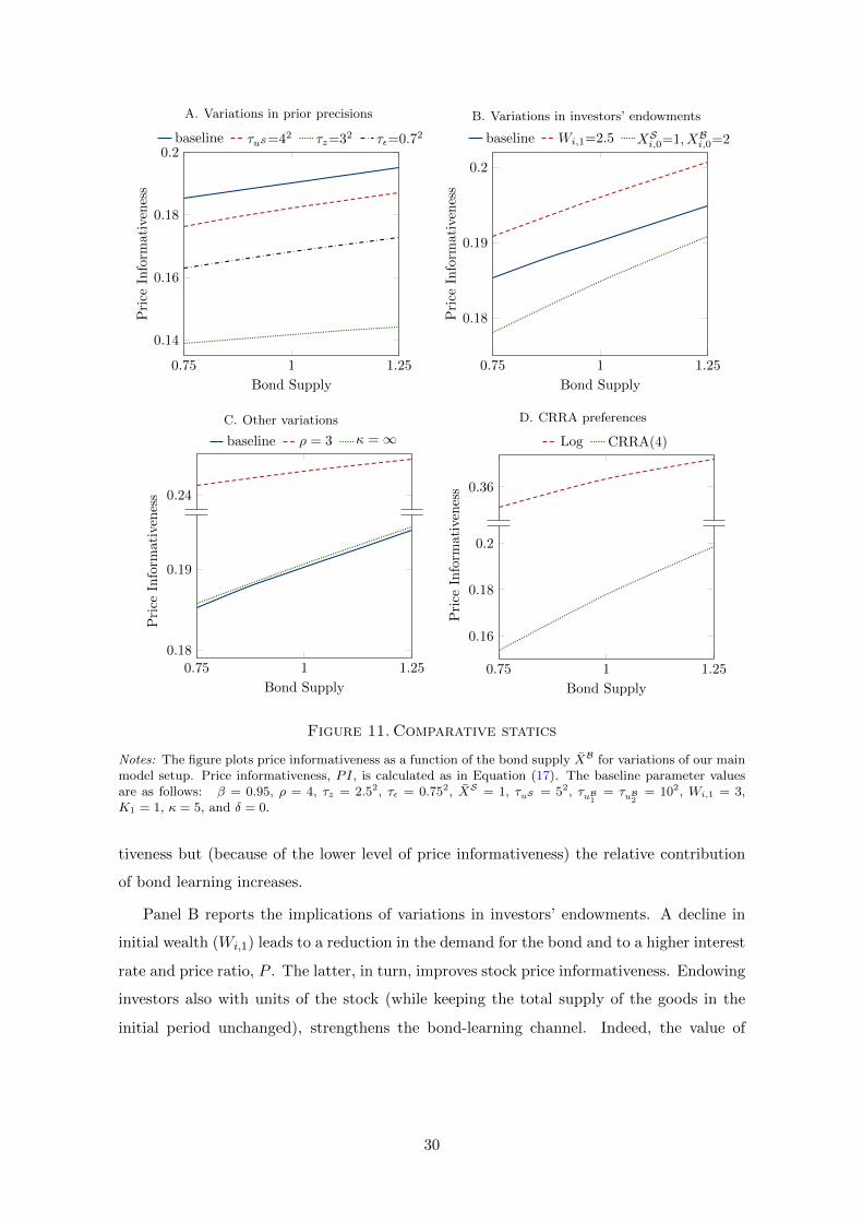
all four panels, price informativeness depends on (specifically, rises in) the bond supply,
confirms a central finding of the paper.
Panel A focuses on the impact of prior precisions. Consistent with the notion that sig-
nals are strategic substitutes, a reduction in the precisions of the noisy stock demand, (τuS ),
of investors’ private signals (τε) and of the fundamental shock (τz) all lower price informa-
29
A. Variations in prior precisions
0.75 1 1.25
0.14
0.16
0.18
0.2
Bond Supply
Price
Inform
ativeness
baseline τuS=42 τz=32 τε=0.72
B. Variations in investors’ endowments
0.75 1 1.25
0.18
0.19
0.2
Bond Supply
Price
Inform
ativeness
baseline Wi,1=2.5 XSi,0=1, XB
i,0=2
C. Other variations
0.24
Price
Inform
ativeness
baseline ρ = 3 κ = ∞
0.75 1 1.250.18
0.19
Bond Supply
D. CRRA preferences
0.36
Price
Inform
ativeness
Log CRRA(4)
0.75 1 1.25
0.16
0.18
0.2
Bond Supply
Figure 11. Comparative statics
Notes: The figure plots price informativeness as a function of the bond supply XB for variations of our mainmodel setup. Price informativeness, PI, is calculated as in Equation (17). The baseline parameter valuesare as follows: β = 0.95, ρ = 4, τz = 2.52, τε = 0.752, XS = 1, τuS = 52, τuB
1= τuB
2= 102, Wi,1 = 3,
K1 = 1, κ = 5, and δ = 0.
tiveness but (because of the lower level of price informativeness) the relative contribution
of bond learning increases.
Panel B reports the implications of variations in investors’ endowments. A decline in
initial wealth (Wi,1) leads to a reduction in the demand for the bond and to a higher interest
rate and price ratio, P . The latter, in turn, improves stock price informativeness. Endowing
investors also with units of the stock (while keeping the total supply of the goods in the
initial period unchanged), strengthens the bond-learning channel. Indeed, the value of
30

investors’ stock endowments, and so their initial wealth, now depends on the bond supply.
This makes the price ratio and, hence, price informativeness more sensitive to the bond
supply (i.e., the curve steepens).
Panel C displays the results of the remaining comparative statics analyses. While shut-
ting down the price-elastic bond-noise component, uB2 , increases price informativeness (as
there is less noise in the system), it has practically no impact on the link between price
informativeness and the bond supply (or the rate of interest). That is, this noise is “neu-
tral” as far as investors’ learning is concerned. A decline in risk aversion (ρ) shifts up the
informativeness of the stock price because investors trade more aggressively on their private
signals. However, the relative contribution of bond learning weakens (i.e., the curve flat-
tens). This is because it makes the stock price and, hence, the price ratio less sensitive to
changes in posterior precisions (thereby weakening the two-way interaction between price
informativeness and the price ratio). Making the output exogenous (κ = ∞) leaves the
impact of the bond signal largely unchanged.
Finally, Panel D demonstrates that our results remain qualitatively unchanged when
investors have CRRA preferences. The case of log utility is particularly instructive as it
implies a constant wealth-consumption ratio (because the income effect perfectly offsets the
substitution effect). Hence, the signal error originating from aggregate consumption (C1) in
the bond market signal (16) vanishes, thereby bringing the model closer to the illustrative
model discussed in Section III. Quantitatively, the impact of the variations in bond supply
is weaker for low levels of relative risk aversion (i.e., for the log case) as a lower risk aversion
limits variation in the price ratio (similar to the case of CARA utility).
V. Extensions: Multiple Signals
To illustrate the general applicability of our key economic mechanism, we now explore two
extensions of our main framework, both of which feature multiple signals. As in our main
model, investors consume in both periods; the interest rate is determined endogenously,
with investors learning from it; and output is endogenous. For ease of exposition, we turn
off the price-elastic bond-noise component (i.e., set uB2 = 0) because, as just shown, it has
no bearing on our key mechanism.
31
V.A. Multiple Risky Assets
In our first extension, we allow for multiple risky assets and focus on the cross-sectional
implications of learning from the interest rate. Beyond generality, this extension brings our
theoretical measure of informational efficiency (so far based on a single firm) closer to the
empirical measure in Section I.
The setting is identical to our main model’s, except for the addition of a second stock.
Specifically, this setting features two stocks, k ∈ 1, 2, with prices P (k), and a risk-free
bond with (endogenous) price 1/Rf . All assets are in finite supplies, denoted by XSk and
XB, respectively. The stocks are modeled as claims to the output of two corresponding
firms, k ∈ 1, 2, which employ the linear production technology (3), with F (k) denoting
output in period 2, z(k) ∼ N (0, τz) productivity shocks, and I(k) real investment. Investors,
i ∈ [0, 1], have CARA utility (4) and receive private signals about each firm’s productivity:
s(k)i = z(k) + ε
(k)i , with ε
(k)i ∼ N (0, τε). Finally, noise traders operate in all three markets,
with demands uSk ∼ N (0, τuS ) and uB1 ∼ N (0, τuB). To highlight the impact of learning
from the bond market, we assume that the two stocks are independent of one another in
terms of fundamentals, private signals, and noise traders’ demand.
To understand the role that learning from the interest rate plays in this economy, note
that aggregating investors’ budget constraints and market clearing delivers a straightforward
two-stock version of the bond market-clearing condition (16). That is, in equilibrium, the
aggregate demand for the three assets plus aggregate consumption must equal aggregate
endowed wealth:
(XS1 − uS1
)P (1) +
(XS2 − uS2
)P (2) +
(XB − uB1
)R−1f + C1 = W1. (20)
Condition (20) has three important implications. First, consistent with the one-stock
model, the bond market provides a signal about the stock demands uSk (i.e., discount rate
news), which allow investors to form more precise (conditional) beliefs about fundamentals.
As before, the error in this signal originates from the bond demand, specifically uB1 , and
aggregate consumption, C1.
Second, a higher interest rate attenuates the noise originating from noise traders’ demand
and, thus, improves the signal’s precision. As a result, stock-price informativeness is again
increasing in the bond supply. Panel A of Figure 12 illustrates this property for price
32
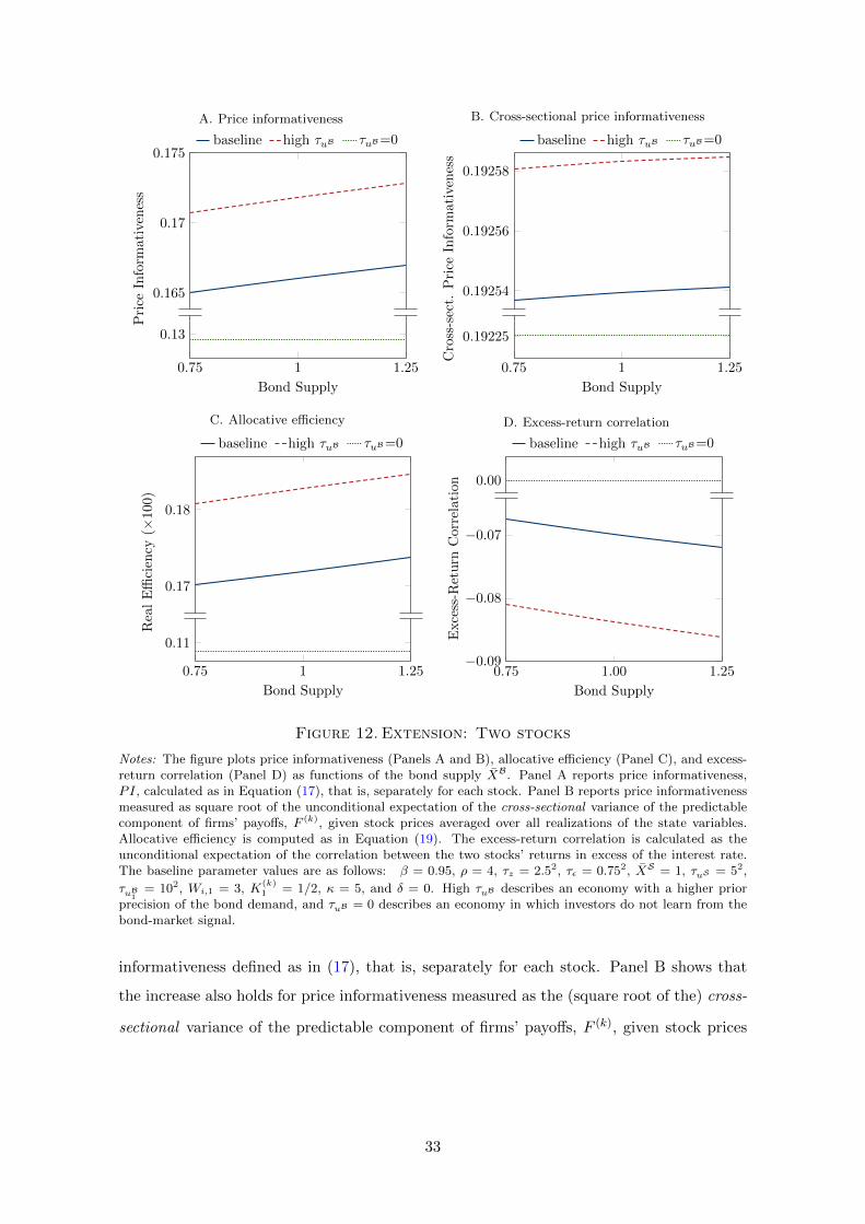
A. Price informativeness
0.165
0.17
0.175Price
Inform
ativeness
baseline high τuB τuB=0
0.75 1 1.25
0.13
Bond Supply
B. Cross-sectional price informativeness
0.19254
0.19256
0.19258
Cross-sect.
Price
Inform
ativeness
baseline high τuB τuB=0
0.75 1 1.25
0.19225
Bond Supply
C. Allocative efficiency
0.17
0.18
Rea
lE
ffici
ency
(×10
0)
baseline high τuB τuB=0
0.75 1 1.25
0.11
Bond Supply
D. Excess-return correlation
0.00
Excess-R
eturn
Correlation
baseline high τuB τuB=0
0.75 1.00 1.25−0.09
−0.08
−0.07
Bond Supply
Figure 12. Extension: Two stocks
Notes: The figure plots price informativeness (Panels A and B), allocative efficiency (Panel C), and excess-return correlation (Panel D) as functions of the bond supply XB. Panel A reports price informativeness,PI, calculated as in Equation (17), that is, separately for each stock. Panel B reports price informativenessmeasured as square root of the unconditional expectation of the cross-sectional variance of the predictablecomponent of firms’ payoffs, F (k), given stock prices averaged over all realizations of the state variables.Allocative efficiency is computed as in Equation (19). The excess-return correlation is calculated as theunconditional expectation of the correlation between the two stocks’ returns in excess of the interest rate.The baseline parameter values are as follows: β = 0.95, ρ = 4, τz = 2.52, τε = 0.752, XS = 1, τuS = 52,
τuB1
= 102, Wi,1 = 3, K(k)1 = 1/2, κ = 5, and δ = 0. High τuB describes an economy with a higher prior
precision of the bond demand, and τuB = 0 describes an economy in which investors do not learn from thebond-market signal.
informativeness defined as in (17), that is, separately for each stock. Panel B shows that
the increase also holds for price informativeness measured as the (square root of the) cross-
sectional variance of the predictable component of firms’ payoffs, F (k), given stock prices
33

(i.e., as in our empirical measure (2)).33 Accordingly, allocative efficiency also improves in
the supply of the bond (Panel C).34
Third, the bond market signal induces a negative correlation between an investor’s beliefs
about the noisy demands of the two stocks, even though the demands are uncorrelated with
one another. In particular, condition (20) constrains the (weighted) sum of the residual
supplies of the two stocks, (XSk − uSk). Hence, conditional on the bond’s noisy demands
and aggregate consumption, an investor who assigns a higher value to one of the stocks’ noisy
demands rationally assigns a lower value to the demand for the other stock. This generates
a negative correlation between an investor’s beliefs about the payoffs of the two stocks,
which, in turn, lowers the correlation of the excess returns of the two stocks. Crucially,
this effect strengthens with the precision of the bond market signal. Hence, the correlation
between excess returns declines (or, put differently, their dispersion rises) in the interest
rate, or, equivalently, in the bond supply (Panel D).35 Notably, in stark contrast to Admati
(1985), the correlation of the excess returns of the two stocks is nonzero despite the stocks’
payoffs, private signal errors, and noisy demands being independent of each other.
As expected, the higher the precision of the noise traders’ bond demand, the stronger
these three effects are. These mounting effects lead to improved informational and allocative
efficiency (Panels A to C) and lower excess-return correlation (Panel D).
V.B. Multiple Price Signals
In our second extension, we allow for multiple price signals. In particular, we demonstrate
that other prices, such as the good’s price (i.e., the rate of inflation), also reveal discount
rate news.
For that purpose, we incorporate money into our single-stock framework and, accord-
ingly, now distinguish between nominal and real quantities. In particular, we assume that
33As expected, the cross-sectional variance and its sensitivity to the bond supply are fairly small becausewe only have two (independent and symmetric) stocks in the model, rather than hundreds of correlatedstocks as in the empirical analysis.
34Note, in our framework, with no constraint on investment, firms’ investment decisions are independentof one another. If aggregate capital is scarce, then the improvement in price informativeness also leads to abetter allocation of capital across firms and, hence, to lower dispersion in the marginal products of capital.
35For ease of exposition, we assume independent payoffs and demands. As a result, the conditionalcorrelation of the two stocks’ excess returns is zero absent learning from the interest rate (τuB
1= 0). To
accommodate a positive correlation between the two stocks (as is typically found in the data), one couldsimply assume positively correlated payoffs (or liquidity demands).
34
investors derive utility from the quantity of the real money balances they hold.36 Formally,
investor i maximizes Ui(Ci,1, Ci,2)− (1/α) exp(−α(XMi /PG1 )
), with parameter α > 0, and
Ui denoting the two-period CARA utility in (4). Here, PGt denotes the price of the good in
period t ∈ 1, 2 (with PG2 being normalized to 1); XMi denotes investor i’s money holdings;
and XMi /PGt denotes her real money balance in period t. Investors’ budget constraints,
accordingly, also account for their real money holdings.37 As with the other assets, the
supply of money, XM, is assumed to be finite. Finally, in addition to their stock and bond
demands, we assume that noise traders have an uncorrelated random demand for money,
uM1 ∼ N (0, 1/τuM), which prevents the price system from being perfectly revealing.38
To understand the role that the good’s price and the interest rate play in this economy,
note that investors’ budget constraints, combined with market clearing, imply the following
two equilibrium conditions:39,40
sB = uS +uB1Rf P
+uM1PG1 P
− C1
Pand sM = uS +
uB1Rf P
+ρ+ α
ρ
uM1PG1 P
, (21)
where sB and sM represent two distinct signals (and, as before, C1 denotes aggregate
consumption). The first equation is the counterpart to the bond market signal (16), to
which noise traders’ (real) money holdings were added; it is the result of market clearing
in the bond market. The second equation—absent from the model without money—can be
interpreted as a money market signal, as it arises from clearing the money market.
Notably, both the bond and the money markets provide signals about the noisy stock
demand, uS . Hence, not only the rate of interest but also the good’s price (or, equivalently,
the rate of inflation, PG2 /PG1 ) reveal discount rate news, which, in turn, allows investors to
form more precise beliefs about the fundamental (i.e., their information set has expanded
to Fi = si, P,Rf , PG1 ). The signal errors originate from the noisy bond demand, uB1 , the
36This is a commonly used shortcut to model the usefulness of money as a medium of exchange; otherwise,money would be dominated as a store of value (to the extent that bonds strictly pay positive nominalinterest). It captures the notion that, the higher the purchasing power of an investor’s money holdings, thelower is the disutility cost associated with exchange, which results in higher overall utility.
37Equations (A18) and (A19) in Appendix B.C.2 display the exact formulation of investors’ optimizationproblem.
38Consistent with our results for the bond market, adding a price-elastic component to noise traders’demand for money does not alter our findings.
39The equilibrium is defined as previously with the addition of the market-clearing condition for money:∫XMi di+ uM1 = XM. Note that, by Walras’ law, clearing in the bond, the stock, and the money markets
guarantees clearing in the goods market.40See Appendix B for the proof and the explicit expressions for sB and sM.
35
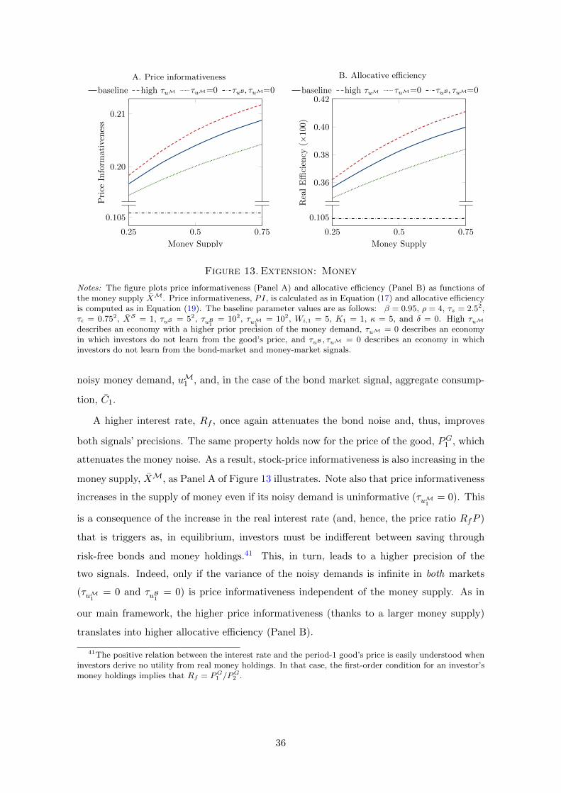
A. Price informativeness
0.20
0.21
Price
Inform
ativeness
baseline high τuM τuM=0 τuB, τuM=0
0.25 0.5 0.75
0.105
Money Supply
B. Allocative efficiency
0.36
0.38
0.40
0.42
Rea
lE
ffici
ency
(×100)
baseline high τuM τuM=0 τuB, τuM=0
0.25 0.5 0.75
0.105
Money Supply
Figure 13. Extension: Money
Notes: The figure plots price informativeness (Panel A) and allocative efficiency (Panel B) as functions ofthe money supply XM. Price informativeness, PI, is calculated as in Equation (17) and allocative efficiencyis computed as in Equation (19). The baseline parameter values are as follows: β = 0.95, ρ = 4, τz = 2.52,τε = 0.752, XS = 1, τuS = 52, τuB
1= 102, τuM
1= 102, Wi,1 = 5, K1 = 1, κ = 5, and δ = 0. High τuM
describes an economy with a higher prior precision of the money demand, τuM = 0 describes an economyin which investors do not learn from the good’s price, and τuB , τuM = 0 describes an economy in whichinvestors do not learn from the bond-market and money-market signals.
noisy money demand, uM1 , and, in the case of the bond market signal, aggregate consump-
tion, C1.
A higher interest rate, Rf , once again attenuates the bond noise and, thus, improves
both signals’ precisions. The same property holds now for the price of the good, PG1 , which
attenuates the money noise. As a result, stock-price informativeness is also increasing in the
money supply, XM, as Panel A of Figure 13 illustrates. Note also that price informativeness
increases in the supply of money even if its noisy demand is uninformative (τuM1= 0). This
is a consequence of the increase in the real interest rate (and, hence, the price ratio RfP )
that is triggers as, in equilibrium, investors must be indifferent between saving through
risk-free bonds and money holdings.41 This, in turn, leads to a higher precision of the
two signals. Indeed, only if the variance of the noisy demands is infinite in both markets
(τuM1= 0 and τuB1
= 0) is price informativeness independent of the money supply. As in
our main framework, the higher price informativeness (thanks to a larger money supply)
translates into higher allocative efficiency (Panel B).
41The positive relation between the interest rate and the period-1 good’s price is easily understood wheninvestors derive no utility from real money holdings. In that case, the first-order condition for an investor’smoney holdings implies that Rf = PG1 /P
G2 .
36

As with bond market noise, the effect is stronger, the more precise the noisy money
demand. In particular, monetary policy might be interpreted as determining not only the
supply of bonds and money (XB and XM) but also the precision of bonds and money
(τuB1and τuM1
).42 Indeed, to the extent that the government or central bank does not
commit to (or communicate) a precise level of debt or money supplies, it adds to the
noise created by liquidity traders. For instance, by disclosing a narrower range of bond
or money supplies (corresponding to a more transparent policy), it enables investors to
know with greater confidence what these supplies are and, thus, enhances the sensitivity
of price informativeness to debt and money supplies.43 This makes policy implementation
more efficient by allowing the government to raise informativeness without actually varying
supplies.
VI. Conclusion
In this paper, we provide new theoretical and empirical insights into how investors use
information contained in interest rates to learn about economic fundamentals and how this
affects informational and allocative efficiency.
We develop a novel noisy rational expectations equilibrium model in which the interest
rate is determined endogenously by supply and demand. We demonstrate that the inter-
est rate reveals information about noise traders’ stock demand (i.e., discount rate news),
which, in turn, allows investors to form more precise beliefs about a stock’s cashflows from
observing the stock’s price. Provided that noise traders’ stochastic bond demand is not too
price-elastic (which we argue is plausible), the strength of this effect is positively related to
the interest rate as a higher interest rate attenuates the error in the bond market signal.
Consequently, both stock-price informativeness and allocative efficiency positively correlate
with long-term rates or, equivalently, bond supply. The robust empirical evidence we report
lends support to this prediction. This mechanism also endogenously creates countercycli-
cality in the price of risk as well as in the volatility and comovement of stock returns, as in
the data.
42Under this interpretation, monetary policy is exogenous and, accordingly, does not convey any infor-mation to investors. Our focus is on how such a policy affects the public’s (as well as the government’s own)ability to learn about economic fundamentals from stock prices. An interesting extension of the model couldbe to endogenize monetary policy, to account for its impact on stock-price informativeness.
43Central bank communication and monetary policy transparency comprise many aspects, and the lit-eratures on both are extensive (for a survey, see Blinder et al. (2008)). Using the (Geraats, 2014, p. 5)classification of transparency, we consider here “policy transparency,” that is, the “communication of thepolicy stance (including the policy decision, policy explanation and inclination with respect to future policyactions).”
37

More broadly, our analyses offer novel insights into the impact of fiscal and monetary
policies in an environment in which information about economic fundamentals is asymmet-
ric across investors. In particular, we show that increases in the supply of (demand for)
both bonds and money improve (harm) informational and allocative efficiency. As such,
our findings highlight novel implications of the strong demand for safe assets observed in
recent decades and point towards important unintended consequences of policies such as
unconventional monetary policy or “financial repression.”44 Our findings also highlight
that more transparent policies (in the sense of more precise disclosures about or of stricter
commitments to bond and money issuance) can improve the stock-market efficiency.
Finally, our findings also suggest a novel interpretation of the concomitant declines in ag-
gregate productivity growth and real interest rates in the United States (Decker et al. 2017)
and in capital allocation efficiency and real interest rates in southern Europe (Gopinath
et al. 2017). Specifically, the decline in interest rates might have impaired investor learn-
ing about economic fundamentals and, hence, made the allocation of capital less efficient,
thereby slowing down productivity growth.45 We look forward to empirical work testing
whether these associations are causal or mere correlations.
44Financial repression refers to policies that force captive domestic audiences (such as pension funds ordomestic banks) to hold government debt and, hence, keep interest rates lower than would otherwise prevail(see, e.g., Reinhart, Kirkegaard and Sbrancia 2011, Chari, Dovis and Kehoe 2020).
45Most of this evidence is on private firms, which can be added to our model in a straightforward fashion.Assume that a private firm employs a similar production technology, with productivity that is correlatedwith the public firm’s (e.g., through economywide shocks). The private firm’s manager then learns aboutthe public firm’s productivity from the stock price and the interest rate (just as the public firm managerdoes), from which she learns about her own productivity. Thus, a higher interest rate facilitates learning forthe private firm and increases the efficiency of the private firm’s investments (as for the public firm).
38
References
Admati, Anat. 1985. “A Noisy Rational Expectations Equilibrium for Multi-asset Secu-
rities Markets.” Econometrica, 53(3): 629–657.
Albagli, Elias, Christian Hellwig, and Aleh Tsyvinski. 2015. “A Theory of Asset
Prices Based on Heterogeneous Information.” Working Paper.
Bai, Jennie, Thomas Philippon, and Alexi Savov. 2016. “Have Financial Markets
Become More Informative?” Journal of Financial Economics, 122(3): 625–654.
Banerjee, Snehal, and Brett Green. 2015. “Signal or noise? Uncertainty and learn-
ing about whether other traders are informed.” Journal of Financial Economics,
117(2): 398–423.
Barlevy, Gadi, and Pietro Veronesi. 2000. “Information Acquisition in Financial Mar-
kets.” Review of Economic Studies, 67(1): 79–90.
Barlevy, Gadi, and Pietro Veronesi. 2003. “Rational Panics and Stock Market
Crashes.” Journal of Economic Theory, 110(2): 234–263.
Bernanke, Ben. 2005. “The Global Saving Glut and the U.S. Current Account Deficit.”
speech delivered at the Sandridge Lecture, Virginia Association of Economists, Rich-
mond, Va., March 10.
Bernanke, Ben, and Mark Gertler. 1989. “Agency Costs, Net Worth, and Business
Fluctuations.” American Economic Review, 79(1): 14–31.
Biais, Bruno, Johan Hombert, and Pierre-Olivier Weill. 2014. “Equilibrium Pric-
ing and Trading Volume under Preference Uncertainty.” Review of Economic Studies,
81(4): 1401–1437.
Biais, Bruno, Peter Bossaerts, and Chester Spatt. 2010. “Equilibrium Asset Pricing
and Portfolio Choice Under Asymmetric Information.” Review of Financial Studies,
23(4): 1503–1543.
Blinder, Alan, Michael Ehrmann, Marcel Fratzscher, Jakob de Haan, and
David-Jan Jansen. 2008. “Central Bank Communication and Monetary Policy: A
Survey of Theory and Evidence.” Journal of Economic Literature, 46(4): 910–945.
Bloom, Nicholas. 2009. “The Impact of Uncertainty Shocks.” Econometrica, 77(3): 623–
685.Bond, Philip, Alex Edmans, and Itay Goldstein. 2012. “The Real Effects of Financial
Markets.” Annual Review of Financial Economics, 4(1): 339–360.
Brennan, Michael J., and Henry H. Cao. 1997. “International Portfolio Investment
Flows.” Journal of Finance, 52(5): 1851–1880.
Breon-Drish, Bradyn. 2015. “On Existence and Uniqueness of Equilibrium in a Class of
Noisy Rational Expectations Models.” Review of Economic Studies, 82(3): 868–921.
Breugem, Matthijs, and Adrian Buss. 2019. “Institutional Investors and Information
Acquisition: Implications for Asset Prices and Informational Efficiency.” Review of
Financial Studies, 32(6): 2260–2301.
Brunnermeier, Markus, and Lasse Heje Pedersen. 2008. “Market Liquidity and
Funding Liquidity.” Review of Financial Studies, 22(6): 2201–2238.
Brunnermeier, Markus K., and Yuliy Sannikov. 2014. “A Macroeconomic Model
with a Financial Sector.” American Economic Review, 104(2): 379–421.
39

Chari, V. V., Alessandro Dovis, and Patrick Kehoe. 2020. “On the Optimality of
Financial Repression.” Journal of Political Economy, 128(2): 710–739.
Danthine, Jean-Pierre, and John Donaldson. 1986. “Inflation and Asset Prices in an
Exchange Economy.” Econometrica, 54(3): 585–605.
Decker, Ryan A., John Haltiwanger, Ron S. Jarmin, and Javier Miranda. 2017.
“Declining Dynamism, Allocative Efficiency, and the Productivity Slowdown.” Ameri-
can Economic Review, 107(5): 322–326.
Dessaint, Olivier, Thierry Foucault, Laurent Fresard, and Adrien Matray.
2018. “Noisy Stock Prices and Corporate Investment.” Review of Financial Studies,
32(7): 2625–2672.
Detemple, Jerome. 2002. “Asset pricing in an intertemporal partially-revealing rational
expectations equilibrium.” Journal of Mathematical Economics, 38(1): 219–248.
Draghi, Mario. 2015. “The ECBs Recent Monetary Policy Measures: Effectiveness and
Challenges.” Camdessus lecture, Washington, DC.
Edmans, Alex, Itay Goldstein, and Wei Jiang. 2015. “Feedback Effects, Asymmetric
Trading, and the Limits to Arbitrage.” American Economic Review, 105(12): 3766–
3797.Eggertsson, Gauti B., Neil R. Mehrotra, and Jacob A. Robbins. 2019. “A Model of
Secular Stagnation: Theory and Quantitative Evaluation.” American Economic Jour-
nal: Macroeconomics, 11(1): 1–48.
Farboodi, Maryam, and Laura Veldkamp. 2019. “Long Run Growth of Financial
Technology.” American Economic Review. forthcoming.
Fisher, Richard. 2013. “Horseshift! (With Reference to Gordian Knots).” National As-
sociation of State Retirement Administrators, Portland, OR.
Foucault, Thierry, and Laurent Fresard. 2014. “Learning from Peers’ Stock Prices and
Corporate Investment.” Journal of Financial Economics, 111(3): 554–577.
Ganguli, Jayant Vivek, and Liyan Yang. 2009. “Complementarities, Multiplicity, and
Supply Information.” Journal of the European Economic Association, 7(1): 90–115.
Geraats, Petra. 2014. “Monetary Policy Transparency.” CESifo Group Munich CESifo
Working Paper Series 4611.
Goldstein, Itay, and Liyan Yang. 2017. “Information Disclosure in Financial Markets.”
Annual Review of Financial Economics, 9(1): 101–125.
Gopinath, Gita, Sebnem Kalemli-Ozcan, Loukas Karabarbounis, and Carolina
Villegas-Sanchez. 2017. “Capital Allocation and Productivity in South Europe.”
Quarterly Journal of Economics, 132(4): 1915–1967.
Gorton, Gary, Stefan Lewellen, and Andrew Metrick. 2012. “The Safe-Asset Share.”
American Economic Review, 102(3): 101–106.
Grossman, Sanford J, and Joseph E Stiglitz. 1980. “On the Impossibility of Informa-
tionally Efficient Markets.” American Economic Review, 70(3): 393–408.
Hellwig, Martin F. 1980. “On the Aggregation of Information in Competitive Markets.”
Journal of Economic Theory, 22(3): 477–498.
He, Zhiguo, and Arvind Krishnamurthy. 2013. “Intermediary Asset Pricing.” Amer-
ican Economic Review, 103(2): 732–770.
40

Kacperczyk, Marcin, Stijn van Nieuwerburgh, and Laura Veldkamp. 2016. “A
Rational Theory of Mutual Funds’ Attention Allocation.” Econometrica, 84(2): 571–
626.Kiyotaki, Nobuhiro, and John Moore. 1997. “Credit Cycles.” Journal of Political
Economy, 105(2): 211–248.
Kodres, Laura E., and Matthew Pritsker. 2002. “A Rational Expectations Model of
Financial Contagion.” Journal of Finance, 57(2): 769–799.
Koeva, Petya. 2000. “The Facts About Time-to-Build.” IMF Working paper.
Krishnamurthy, Arvind, and Annette Vissing-Jorgensen. 2012. “The Aggregate
Demand for Treasury Debt.” Journal of Political Economy, 120(2): 233–267.
LeRoy, Stephen F. 1984a. “Nominal Prices and Interest Rates in General Equilibrium:
Endowment Shocks.” Journal of Business, 57(2): 197–213.
LeRoy, Stephen F. 1984b. “Nominal Prices and Interest Rates in General Equilibrium:
Money Shocks.” Journal of Business, 57(2): 177–195.
Lowenstein, Mark, and Gregory A. Willard. 2006. “The Limits of Investor Behavior.”
Journal of Finance, 61(1): 231–258.
Lucas, Robert E. 1982. “Interest Rates and Currency Prices in a Two-Country World.”
Journal of Monetary Economics, 10(3): 335–359.
Manzano, Carolina, and Xavier Vives. 2011. “Public and Private Learning from Prices,
Strategic Substitutability and Complementarity, and Equilibrium Multiplicity.” Jour-
nal of Mathematical Economics, 47(3): 346 – 369.
Marshall, David A. 1992. “Inflation and Asset Returns in a Monetary Economy.” Journal
of Finance, 47(4): 1315–1342.
Mian, Atif, Ludwig Straub, and Amir Sufi. 2021. “What Explains the Decline in r∗?
Rising Income Inequality versus Demographic Shifts.” Working paper, University of
Chicago.
Newey, Whitney K., and Kenneth D. West. 1994. “Automatic Lag Selection in Co-
variance Matrix Estimation.” Review of Economic Studies, 61(4): 631–653.
Peress, Joel. 2004. “Wealth, Information Acquisition, and Portfolio Choice.” Review of
Financial Studies, 17(3): 879–914.
Powell, Jerome. 2017. “Low Interest Rates and the Financial System.” speech delivered
at the Annual Meeting of the American Finance Association, Chicago, IL.
Rampini, Adriano A., and S. Viswanathan. 2010. “Collateral, Risk Management, and
the Distribution of Debt Capacity.” Journal of Finance, 65(6): 2293–2322.
Reinhart, Carmen, Jacob Kirkegaard, and Belen Sbrancia. 2011. “Financial Re-
pression Reduc.” Finance and Development, 2(48).
Sellin, Peter. 2001. “Monetary Policy and the Stock Market: Theory and Empirical Evi-
dence.” Journal of Economic Surveys, 15(4): 491–541.
Svensson, Lars. 1985. “Money and Asset Prices in a Cash-in-Advance Economy.” Journal
of Political Economy, 93(5): 919–944.
The Economist. 2020. “Emerging markets launch QE, too.” The Economist.
Tobin, James. 1969. “A General Equilibrium Approach To Monetary Theory.” Journal
of Money, Credit and Banking, 1(1): 15–29.
41

van Nieuwerburgh, Stijn, and Laura Veldkamp. 2009. “Information Immobility and
the Home Bias Puzzle.” Journal of Finance, 64(3): 1187–1215.
van Nieuwerburgh, Stijn, and Laura Veldkamp. 2010. “Information Acquisition and
Under-Diversification.” Review of Economic Studies, 77(2): 779–805.
Verrecchia, Robert E. 1982. “Information Acquisition in a Noisy Rational Expectations
Economy.” Econometrica, 50(6): 1415–1430.
Watanabe, Masahiro. 2008. “Price Volatility and Investor Behavior in an Overlapping
Generations Model with Information Asymmetry.” Journal of Finance, 63(1): 229–272.
Yang, Liyan, and Haoxiang Zhu. 2019. “Back-Running: Seeking and Hiding Funda-
mental Information in Order Flows.” Review of Financial Studies, 33(4): 1484–1533.
42
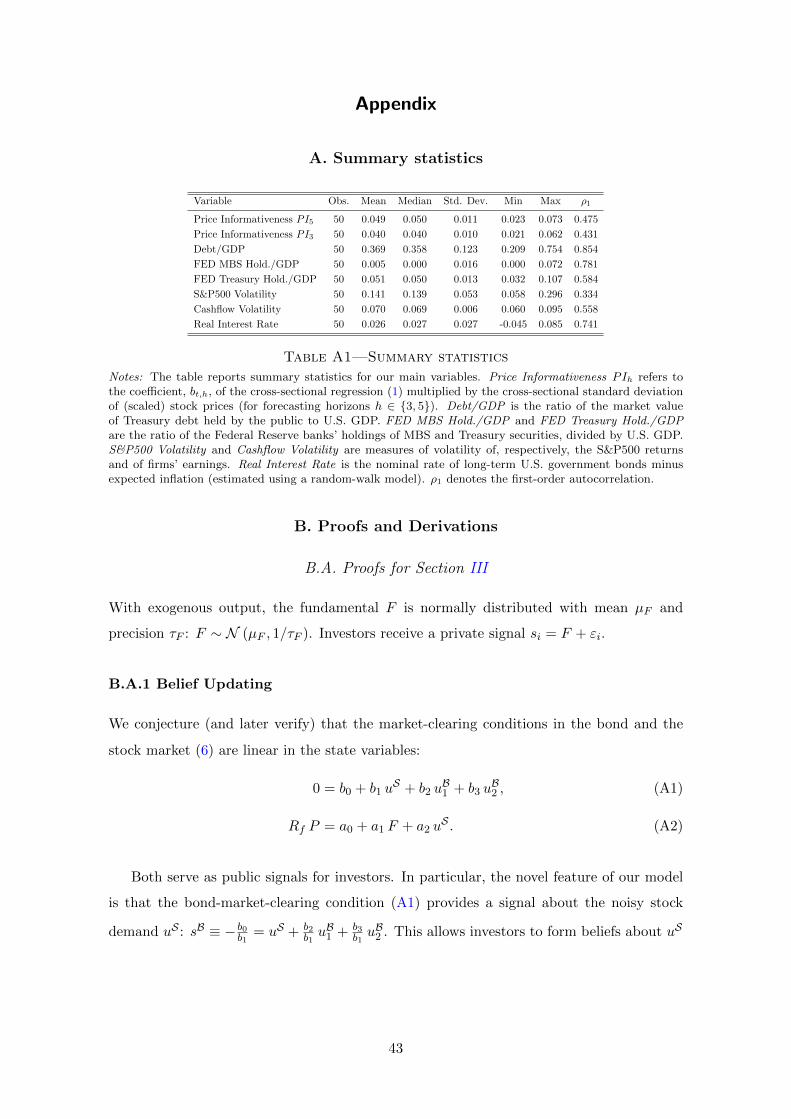
Appendix
A. Summary statistics
Variable Obs. Mean Median Std. Dev. Min Max ρ1
Price Informativeness PI5 50 0.049 0.050 0.011 0.023 0.073 0.475
Price Informativeness PI3 50 0.040 0.040 0.010 0.021 0.062 0.431
Debt/GDP 50 0.369 0.358 0.123 0.209 0.754 0.854
FED MBS Hold./GDP 50 0.005 0.000 0.016 0.000 0.072 0.781
FED Treasury Hold./GDP 50 0.051 0.050 0.013 0.032 0.107 0.584
S&P500 Volatility 50 0.141 0.139 0.053 0.058 0.296 0.334
Cashflow Volatility 50 0.070 0.069 0.006 0.060 0.095 0.558
Real Interest Rate 50 0.026 0.027 0.027 -0.045 0.085 0.741
Table A1—Summary statistics
Notes: The table reports summary statistics for our main variables. Price Informativeness PIh refers tothe coefficient, bt,h, of the cross-sectional regression (1) multiplied by the cross-sectional standard deviationof (scaled) stock prices (for forecasting horizons h ∈ 3, 5). Debt/GDP is the ratio of the market valueof Treasury debt held by the public to U.S. GDP. FED MBS Hold./GDP and FED Treasury Hold./GDPare the ratio of the Federal Reserve banks’ holdings of MBS and Treasury securities, divided by U.S. GDP.S&P500 Volatility and Cashflow Volatility are measures of volatility of, respectively, the S&P500 returnsand of firms’ earnings. Real Interest Rate is the nominal rate of long-term U.S. government bonds minusexpected inflation (estimated using a random-walk model). ρ1 denotes the first-order autocorrelation.
B. Proofs and Derivations
B.A. Proofs for Section III
With exogenous output, the fundamental F is normally distributed with mean µF and
precision τF : F ∼ N (µF , 1/τF ). Investors receive a private signal si = F + εi.
B.A.1 Belief Updating
We conjecture (and later verify) that the market-clearing conditions in the bond and the
stock market (6) are linear in the state variables:
0 = b0 + b1 uS + b2 u
B1 + b3 u
B2 , (A1)
Rf P = a0 + a1 F + a2 uS . (A2)
Both serve as public signals for investors. In particular, the novel feature of our model
is that the bond-market-clearing condition (A1) provides a signal about the noisy stock
demand uS : sB ≡ − b0b1
= uS + b2b1uB1 + b3
b1uB2 . This allows investors to form beliefs about uS
43

conditional on signal sB, with conditional precision τuS |sB ≡ Var(uS | sB
)−1and conditional
mean µuS |sB = E[uS | sB
]:
τuS |sB = τuS +b21
b22τuB1
+b23τuB2
, and µuS |sB =1
τuS |sB
b21b22τuB1
+b23τuB2
(−b0b1
). (A3)
Combining these conditional beliefs about the noisy stock demand with an investor’s prior
information about F , her private signal si = F + εi, and the conjectured stock price signal
RfP , in (A2), yields her posterior beliefs about the stock payoff F :
τ ≡ Var(F | si, Rf , P )−1 = τF + τε +a2
1
a22
τuS |sB ; and (A4)
E [F | si, Rf , P ] =τFτµF +
τετsi +
τuS |sB
τ
a21
a22
RfP − a0 − a2 µuS |sB
a1(A5)
=1
τ
(τFµF −
a1
a22
τuS |sB(a0 + a2 µuS |sB
))+τετsi +
τuS |sB
τ
a1
a22
RfP.
B.A.2 Individual Optimization
In the absence of initial consumption, the objective of investor i is to choose her portfolio
holdings in the stock, XSi , and in the bond, XBi , to maximize the expected utility from
terminal consumption Ci,2:
Ui(Ci,2) = −(1/ρ)E[exp(−ρCi,2
) ∣∣Fi] , (A6)
subject to the budget constraints:
XSi P +XBi R−1f = Wi,1 and Ci,2 = XSi F +XBi . (A7)
Solving the period-1 budget equation (5) (setting Ci,1 = 0) for the bond holdings, XBi ,
yields
XBi = Rf(Wi,1 −XSi P
), (A8)
which can be used to rewrite the period-2 budget constraint in (5) as
Ci,2 = Rf Wi,1 +XSi (F −Rf P ) . (A9)
44

Plugging the period-2 consumption (A9) into the investor’s utility function and maxi-
mizing the utility with respect to XSi yields the traditional CARA optimal stock demand:
XSi =E[F | si, Rf , P ]− P RfρVar(F | si, Rf , P )
. (A10)
Equations (A8) and (A10) jointly characterize investors’ optimal portfolios.
B.A.3 Market Clearing
Aggregating investors’ bond demand (A8) and imposing market clearing in the stock and
bond markets implies∫ 1
0XBi di+ uB1 + uB2 Rf =
∫ 1
0Rf
(Wi,1 −XSi P
)di+ uB1 + uB2 Rf
= Rf W1 −(XS − uS
)P Rf + uB1 + uB2 Rf , XB.
This verifies conjecture (A1) and (by matching coefficients) directly yields
b0 = Rf(W1 − XS P
)− XB, b1 = P Rf , b2 = 1, and b3 = Rf . (A11)
As a result, investors’ conditional mean and precision about the noisy stock demand in (A3)
are given by
τuS |sB = τuS +P 2
1R2f τuB1
+ 1τuB2
, and (A12)
µuS |sB = − 1
τuS |sB
P1
R2f τuB1
+ 1τuB2
(W1 − XSP − XBR−1
f
). (A13)
45

Plugging investors’ posterior beliefs (A4) and (A5) regarding the payoff F into the stock
demand (A10), aggregating across investors, and imposing market clearing yields∫ 1
0XSi di+ uS
=
∫ 1
0
τ
ρ
1
τ
(τFµF −
a1 τuS |sB
a22
(a0 + a2µuS |sB
))+τετsi +
τuS |sB
τ
a1
a22
RfP −RfPdi+ uS
=1
ρ
(τFµF −
a1τuS |sB
a22
(a0 + a2µuS |sB
))+τετF +
1
ρ
(a1τuS |sB
a22
− τ)RfP + uS , XS ,
(A14)
which validates conjecture (A2). Finally, matching the coefficients of (A14) to those in the
conjecture (A2) and solving the resultant equation system for a0, a1, and a2, yields
a0 =τFτµF +
τε τuS |sB
ρ τµuS |sB , (A15)
a1 =τε
(ρ2 + τε τuS |sB
)τ ρ2
, and a2 = −τε
(ρ2 + τε τuS |sB
)τ ρ2
ρ
τε. (A16)
Hence, investors’ posterior precision about F in (A4) is given by
τ = τF + τε +τ2ε
ρ2τuS |sB . (A17)
Theorem 1 readily follows from (a) plugging coefficients (A11) into the conjecture for
the bond-market-clearing condition (A1), (b) plugging coefficients (A15) and (A16) into
the conjecture for the stock-market-clearing condition (A2), (c) the optimal bond and stock
demand (A8) and (A10), and (d) posterior beliefs (A12), (A13), and (A17).
Lemmas 1 and 2 immediately follow from (A12) and (A13), and from (A17), respec-
tively.
Remark 1 : If investors are also endowed with holdings of the stock (in addition to units of
the good or, equivalently, of a (maturing) bond), then the derivations are unchanged but
for the coefficient b0 which becomes
b0 = Rf(XS0 P + XB0 − XS P
)− XB,
46

where XS0 ≡∫ 1
0 XSi,0 di and XB0 ≡∫ 1
0 XBi,0 di denote the aggregate endowment in stocks and
goods (or, equivalently, maturing bonds), respectively. All other quantities, in particular the
investors’ conditional precision regarding the noisy stock demand (τuS |sB), their posterior
precision (τ), and price informativeness ((τ2ε /ρ
2) τuS |sB), remain unchanged.
B.B. Derivations for Section IV
Solving the period-1 budget constraint in (5) for the bond holdings, XBi , yields
XBi = Rf(Wi,1 −XSi P − Ci,1
).
Aggregating investors’ bond demand and imposing market clearing in the bond and stock
markets implies∫ 1
0XBi di+ uB1 + uB2 Rf =
∫ 1
0Rf
(Wi,1 −XSi P − Ci,1
)di+ uB1 + uB2 Rf
= Rf W1 −RfP(XS − uS
)−Rf C1 + uB1 + uB2 Rf , XB,
where W1 ≡∫ 1
0 Wi,1di and C1 =∫ 1
0 Ci,1 di, respectively, denote aggregate endowed wealth
and aggregate initial consumption. This immediately yields Equation 16.
Taking the first-order condition of the expected firm value, E [v(z, I) |Rf , P ], with re-
spect to real investment, I, yields
−1 + E[(1 + z)− κ
K1I
∣∣∣∣P,Rf] = 0,
which is equivalent to Equation 18.
B.C. Derivations for Section V
Keep in mind that for the frameworks presented in Section V, we turn off the second noise
component; that is, uB2 = 0.
47

B.C.1 Derivations for Section V.A
The objective of each investor i is to maximize her expected CARA utility (4), conditional
on her information set Fi = s(1)i , s
(2)i , Rf , P
(1), P (2) and subject to the following budget
constraints:
Ci,1 +XS1i P (1) +XS2i P (2) +XBi R−1f = Wi,1, and Ci,2 = XS1i F (1) +XS2i F (2) +XBi ,
where XSki denotes the number of shares of stock k held by investor i.
Accordingly, investor i’s demand for the bond can be written as
XBi = Rf
(Wi,1 −XS1i P (1) −XS2i P (2) − Ci,1
).
Aggregating this demand across investors and imposing market clearing in all three markets
then yields
Rf W1 −Rf(XS1 − uS1
)P (1) −Rf
(XS2 − uS2
)P (2) −Rf C1 + uB1 = XB,
which is equivalent to Equation 20.
B.C.2 Derivations for Section V.B
The objective of each investor i is to maximize expected utility
− 1
ρexp(−ρCi,1
)+ β E
[−1
ρexp(−ρCi,2
) ∣∣Fi]− 1
αexp
(−α
(XMi /PG1
)), (A18)
subject to the budget constraints:
Ci,1 +XSi P +XBi R−1f +
XMiPG1
= Wi,1, and Ci,2 = XSi F +XBi +XMiPG2
. (A19)
Combining the budget constraints in (A19), plugging the resultant period-2 consumption
into the investor’s utility function (A18), and deriving the first-order conditions with respect
48

to period-1 consumption, Ci,1, and money holdings, XMi , yields
exp (−ρCi,1) = β Rf E[exp (−ρCi,2)
∣∣Fi] , and
exp
(−αX
Mi
PG1
)= β Rf E
[exp (−ρCi,2)
∣∣Fi] (1− PG1Rf P
G2
),
where the second equation can be simplified to
− α XMi
PG1= −ρCi,1 + ln
(1− PG1
Rf PG2
). (A20)
Substituting out period-1 consumption from first-order condition (A20) (thanks to
(A19)), aggregating across investors, and clearing the stock, bond, and goods markets yields
− α
PG1
(XM − uM
)= ln
(1− PG1
Rf PG2
)(A21)
− ρ(W1 −
(XS − uS
)P −
(XB − uB1
)R−1f −
(XM − uM
) (PG1)−1),
where W1 ≡∫ 1
0 Wi,1di denotes the aggregate endowed wealth.
Simplifying Equation (A21) yields
(1 +
α
ρ
)XM − uM
PG1= −1
ρln
(1− PG1
Rf PG2
)+ W1 −
(XS − uS
)P − XB − uB1
Rf,
which, after defining sM ≡ ρ+αρ
XM
PG1 P+ XS + XB
Rf P+ 1
ρ1P ln
(1− PG1
Rf PG2
)− W1
P yields the
signal sM in (21).
In addition, aggregating investors’ period-1 budget constraint in (A19) and imposing
market clearing in all three markets yields
C1 +(XS − uS
)P +
(XB − uB1
)R−1f +
(XM − uM
) (PG1)−1
= W1, (A22)
which, after defining sB ≡ XS + XB
Rf P+ XM
PG1 P− 1
P W1, yields the signal sB in (21).
49

C. Numerical Solution Approach
The main difficulty in identifying the equilibrium in the presence of intertemporal con-
sumption choices is that the market-clearing conditions in the stock and bond markets are
nonlinear functions of the state variables, with unknown functional forms. As a result, one
cannot explicitly compute the investors’ posterior beliefs and, hence, cannot find a closed-
form solution for the equilibrium. Accordingly, the model must be solved numerically.
For that purpose, we extend the numerical solution approach presented in Breugem
and Buss (2019) to allow for learning from the interest rate, two-period consumption, and
endogenous output. The approach allows for arbitrary price and demand functions, that
is, one does not need to parameterize (conjecture) these functions in any form. Also, it
identifies the equilibrium exactly, up to a discretization of the state space (which can be
made arbitrarily narrow). The algorithm comprises the following four key steps.
First, we discretize the state space into a grid of Nz, NuS , and NuB realizations of the
random variables z, uS , and uB, respectively.46
Second, we form, for any given grid point Ω = zn, uSm, uBo , n ∈ 1, . . . , Nz, m ∈1, . . . , NuS, o ∈ 1, . . . , NuB, the system of equations that characterizes the equilibrium.
The system comprises investors’ first-order conditions with respect to bond and stock hold-
ings, plus the two market-clearing conditions (6) and the optimal real investment condition
(18). Specifically, to accommodate investors’ dispersed signal realizations, we form NS
groups of investors (“signal realization groups”) for each grid point Ω, with each group
receiving a different signal Ss, s ∈ 1, . . . , NS. Thus, we arrive at an equation system
with NS × 2 + 3 equations, with unknowns: Rf (Ω), P (Ω), I(Ω), and XSs (Ω), XBs (Ω),∀s ∈ 1, . . . , NS (i.e., 3 +NS × 2 unknowns in total).
Third, we complement the equation system with a set of equations that characterize
investors’ rational expectations.47 Specifically, for each signal-realization group s and each
“conjectured” level of productivity zw, w ∈ 1, . . . , Nz, we add equations that, under the
beliefs of group s and conditional on prices, describe the aggregate demand for the two
46We truncate the realizations of the bond demand, uB, such that XB − uB ≥ 0. This is needed because,under CARA preferences, the equilibrium might not exist for XB − uB < 0, because of the violation of theInada conditions.
47If investors’ posterior probabilities were exogenous (e.g., a function of private signals or prior beliefsonly), one could directly solve the equation system described in step 2. However, under rational expectations,investors’ beliefs depend on the prices of the two assets. This dependence gives rise to a fixed-point problem.
50

0.75 1 1.250.18
0.19
0.2
Bond Supply
Price
Inform
ativen
ess
baseline 3 st.devs more gridpoints
Figure A1.Grid precision
Notes: The graph plots price informativeness, calculated as in (17), as a function of the bond supply, XB.The graph is based on the following baseline parameter values: β = 0.95, ρ = 4, τz = 2.52, τε = 0.752,XS = 1, τuS = 52, τuB
1= τuB
2= 102, Wi,1 = 3, K1 = 1, κ = 5, and δ = 0. “3 st.devs” denotes computations
with a grid that spans three standard deviations for all state variables, and “more gridpoints” denotescomputations with additional grid points along all dimensions.
assets.48,49 This requires solving for the optimal asset demands of all signal realization
groups and all conjectured levels of productivity, conditional on prices, and aggregating
the resultant demands. This adds N2S × Nz × 2 equations for each grid point Ω, though
many of those are redundant (i.e., can be removed). Based on the conjectured aggregate
demands, uSw, uBw, each group s can then compute her posterior probabilities (employed in
the first-order conditions) for all conjectured levels of productivity zw, w ∈ 1, . . . , Nz,using the distribution of the noise traders’ bond and stock demands.50
Fourth, for each grid point Ω, we solve the resultant large-scale fixed-point problem
using Mathematica. We thereby rely on FindRoot, which uses a dampened version of the
Newton-Raphson method, together with finite differences to compute the Hessian.
We find that the solution of the system is very accurate for Nz = NuS = NuB = 5,
NS = 31, and Nz = 31. Based on that grid, solving the system of equations for one
48To distinguish between the actual values of productivity and asset demands at a given grid point,zn, uSm, uBo , and conjectured productivity and demands, zn, uSm, uBo , we denote the latter with a hat.
49To allow for conjectured productivity to cover a wide range around the actual productivity zn, we createa separate grid specific to conjectured productivity, with entries z1, . . . , zNz.
50Formally, the posterior probability of group s for productivity zw′ , conditional on prices and her privatesignal Ss, is given by
P (zw′ |Rf , P, Ss) =fuS
(uSw′)fuB
(uBw′)fz (zw′ |Ss)∑Nz
w=1 fuS (uSw) fuB (uBw) fz (zw |Ss),
where fz, fuS , and fuB denote the exact density functions of productivity z, the noisy stock demand uS ,and the noisy bond demand uB, respectively.
51

grid point takes about 0.8 seconds on an Intel Core i7 workstation. Hence, solving it
for all 729 grid points requires less than 10 minutes.51 Further increasing the number of
discretization points hardly changes the solution. Figure A1 illustrates this by plotting price
informativeness as a function of the bond supply for computations with a narrower grid.
51To verify the solution approach, we (a) replicate our closed-form solution for the economy without initialconsumption (see Section III), (b) replicate the Hellwig (1980) solution in an economy without learning fromthe interest rate and without initial consumption, and (c) confirm that the solution converges to the solutionwithout private information as τε converges to zero.
52